Assessment and Prediction of Groundwater usingGeospatial and ANN modelingAnkita Pran Dadhich  ( ankitadadhich@mnit.ac.in )

Malaviya National Institute of TechnologyRohit Goyal 

Malaviya National Institute of TechnologyPran Nath Dadhich 

Poornima Institute of Engineering and Technology

Research Article

Keywords: Groundwater, ARIMA, Arti�cial neural network, Water quality, Geospatial, Phagi

Posted Date: April 15th, 2021

DOI: https://doi.org/10.21203/rs.3.rs-246464/v1

License: This work is licensed under a Creative Commons Attribution 4.0 International License.  Read Full License

Assessment and Prediction of Groundwater using Geospatial and ANN modeling

Ankita P. Dadhich1, Rohit Goyal1, Pran N. Dadhich2

1Department of Civil Engineering, Malaviya National Institute of Technology, J.L.N. Marg,

Jaipur 302017, (Rajasthan) INDIA

2Department of Civil Engineering, Poornima Institute of Engineering & Technology, ISI-2,

RIICO Institutional Area, Sitapura, Jaipur 302022 (Rajasthan), INDIA

Email: ankitadadhich@mnit.ac.in, rgoyal.ce@mnit.ac.in, pran.dadhich@poornima.org

Abstract

In semi-arid regions the deterioration in groundwater quality and drop in water level upshots

the importance of spatio-temporal mapping with geospatial and advanced modeling techniques.

In present study, changes in water level, water quality trend patterns and future scenarios of

groundwater in 171 villages of Phagi tehsil, Jaipur district was assessed using eight years

(2012-2019) groundwater data. Spatial interpolation maps were drawn using kriging method

for pre-monsoon season and integrated with three different time series forecasting models

(Simple Exponential Smoothing, Holt's Trend Method, ARIMA) and Artificial Neural Network

models to ascertain the optimal prediction for groundwater level and quality parameters.

Results reveal that the use of ANN model can describe the behavior of groundwater level and

quality parameters more accurately than time series forecasting models. In addition, different

ANN algorithms were tested to select the best-performing algorithm and ANN15 is found the

most accurate one in simulating the magnitude and patterns of pre-monsoon water level data

for year 2019 with R2 = 0.98, and NSE = 0.81. The change in groundwater table was observed

with more than 4.0m rise in 81 villages during 2012-2013 whereas ANNpredicted results of

2023-2024 infer no rise in water table (>4.0m). Water level drop of more than 6.0m was

observed in 16 villages of Phagi tehsil based on predicted results of 2024. Assessment of

groundwater quality parameters like Total dissolved solids, chloride, fluoride and nitrate

indicate chemically unsuitable groundwater for drinking purpose in most part of the Phagi.

ANNpredictions point out excess nitrate content in 58% villages however, Water quality Index

reveals unfit groundwater in 74% villages for human consumption in 2024. This time series

and projected outcome of groundwater at village level can assist the planners and decision-

makers for proper management of groundwater risk areas.

Keywords- Groundwater; ARIMA; Artificial neural network; Water quality;

Geospatial; Phagi

1 Introduction

In arid and semi-arid environment where rainfall is scanty and highly variable with very high

evaporation rate; groundwater is the vital local source for drinking, agricultural, industrial and

domestic uses. Groundwater is generally considered better than surface water because of its

higher quality, less evapo-transpiration and less susceptible to contamination (Chenini and Ben

2010; Kumar et al. 2016). In the last few decades, the availability of ground water is at a greater

risk in Rajasthan state of India due to growing population, urbanization, and large quantities of

groundwater withdrawal for crop production. Over-exploitation of groundwater resources and

drought events have caused severe drop in water table level of Rajasthan. Acute water crisis

could be observed in many parts of Rajasthan especially during the summer months. The

variations in the groundwater level reflects the impact of climatic condition, groundwater

consumption, water storage and other human activities (Minville et al. 2010; Ghazavi et al.

2012); hence groundwater level fluctuation is an important indicator of the ecology and

hydrology of the arid region (Jolly et al. 2008).

The groundwater quality of a region worsens due to geochemical reactions in the

aquifers/soils during its transportation through canals/drainages, and excessive use of chemical

fertilizers and pesticides (Singh et al. 2013; Rawat et al. 2018). The use of such contaminated

water may lead to variety of water borne diseases, hence periodic monitoring and assessment

of groundwater resources becomes necessary to determine the impact of human activities on

groundwater deterioration (Gautam et al. 2018).

In areas with shortage of surface waterbodies, development of different management

strategies for groundwater resource is emerging as an area of great concern in recent decades.

Geospatial technique can be the powerful tool for finding the solutions related to groundwater

resources problems such as determining water availability, rise and drop in water level,

assessing water quality, monitoring, modeling, estimation of the contaminant concentrations in

locations that lack measurement data (Gharbia et al. 2016) and efficient use of groundwater

resources at local or regional scale (Srivastava et al. 2012; Verma et al. 2017). Apart from this

the detailed spatial and temporal trend patterns of groundwater quality and quantity over a

certain period of time using geospatial techniques, could provide reliable, efficient, cost

effective and sustainable management measures. With the availability of soft computing

techniques, different models could be adopted to understand the scenarios of groundwater for

both quantity and quality (Nas and Berktay 2010; Charulatha et al. 2017).

Few research studies (Yesilnacar et al. 2008; Mohanty et al. 2010; Sunayana et al.

2019) suggest that neural network models could help in predicting the groundwater quality and

groundwater level well in advance for understanding the future scenario. Artificial neural

network (ANN) models have also been applied to the water quality problems by several

researchers (Singh et al. 2009; Ay and Kisi 2012; Csábrági et al. 2017). Present study is

confined to semi-arid rural region (Phagi tehsil) of Jaipur district in Rajasthan state. In Phagi

tehsil most of the population is dependent on groundwater for their domestic and agriculture

needs. The groundwater quality of the study area is under stress of severe pollution (Singh et

al.2012; Sharma et al. 2015), hence deterioration in groundwater quality and drop in water level

marks the importance of spatio-temporal mapping with geospatial interpolation technique.

Geospatial technique can evaluate the groundwater risk areas of a region even with the

availability of limited sample points (measured data). Therefore, it is imperative to understand

the water quality trend patterns, changes in groundwater level and future scenarios of

groundwater quality and quantity in Phagi tehsil. The aim of this research is: 1) to ascertain the

spatial and temporal variations in the groundwater level and groundwater quality of Phagi tehsil

during last 8 years (2012 to 2019) by developing spatial interpolation maps; 2) modeling of

water level and important water quality parameters using time series forecasting & ANN

models and identification of optimum model based on model validation using historic data; 3)

to predict the groundwater level changes and groundwater quality during 2019 to 2024 using

the best forcasting model identified for understanding the variations with space and time at

village level.

2 Material and Methods

2.1 Study Area

Phagi Tehsil is located in Jaipur district of Rajasthan state. It covers geographical area of

1,114.3 km2 and extending between north latitudes 26o 25’ and 26o 50’ and east longitudes 75o

20’ and 75o 50’ and forms south western part of the Jaipur District. According to 2011 Census,

there are 32 gram panchayat, 22,713 households with total population of 161,610 and 145 per

km2 population density. The average elevation of study area is 383 m and drained by two

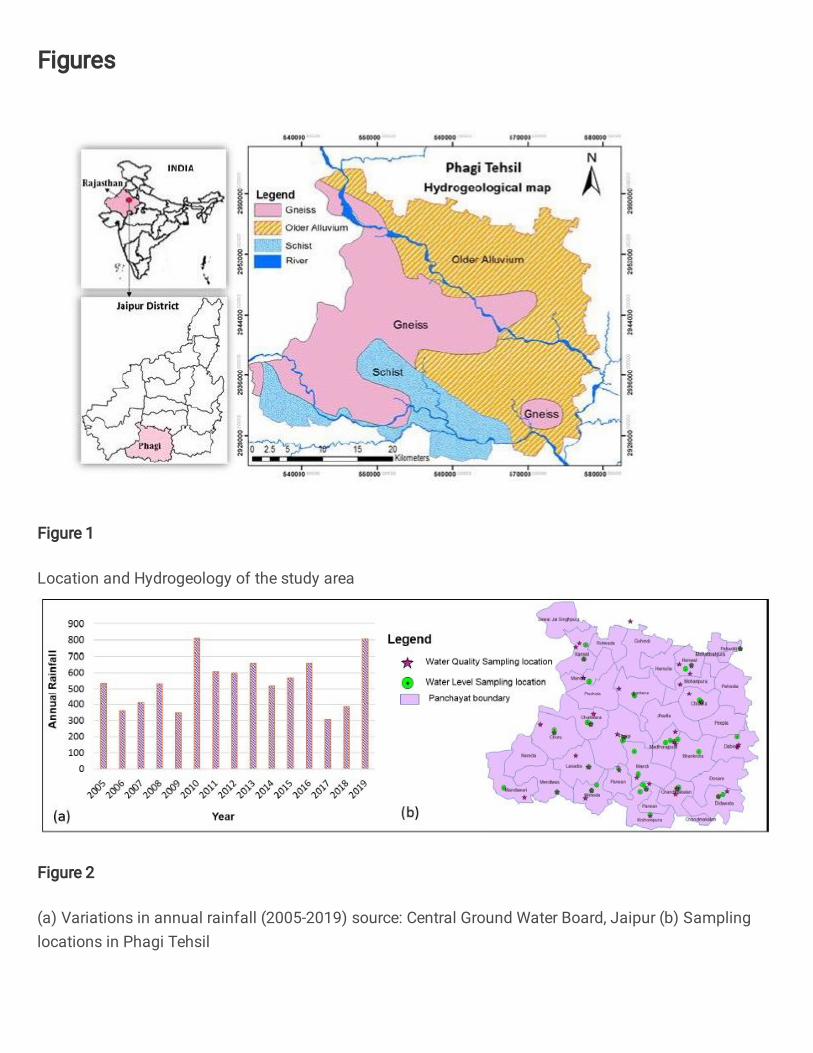
ephemeral rivers viz. Bandi river and Mashi river (Fig. 1). Geomorphologically, Phagi tehsil is

Fig. 1 Location and Hydrogeology of the study area

characterized by undulating plains and pediments with thin to thick soil cover forming flat

gneissic outcrops. The climate of Phagi is semi arid and temperatures vary from 5 to 48o

Celsius. More than 90% annual rainfall is received during monsoon season. Annual average

rainfall during the period 2005 to 2019 has been 539.89mm (Fig. 2a) in Phagi tehsil. The depth

of groundwater varies from 3 to 45m below ground level (bgl) in study area.

Fig. 2 (a) Variations in annual rainfall (2005-2019) source: Central Ground Water Board,

Jaipur (b) Sampling locations in Phagi Tehsil

2.1.1 Hydrogeology of the study area

Fig. 1 shows the hydrogeology of the Phagi tehsil. Gneisses and schists of Bhilwara Super

Group are the oldest rock types. Hard rocks of Bhilwara Super Group, comprising of granulitic

gneisses, quartz, mica, schist, phyllite along with granite and pegmatite intrusives, form main

aquifers in Phagi tehsil. Groundwater at shallow depth occurs under water table condition and

under semi-confined conditions at depth (CGWB 2017).

2.2 Data Collection

The pre-monsoon data was collected for groundwater level and groundwater quality from State

Ground Water Department (SGWD), Jaipur during 2012 to 2019 for different sampling

locations (Fig. 2b) within the Phagi tehsil. The source of all the water level sampling locations

was dug wells and piezometric wells however, water quality samples were collected from hand

pumps, bore well and wells. The sampling locations were plotted in GIS environment using

World Geodetic System (WGS) 1984 as datum and Universal Transverse Mercator (UTM)

Zone 43 North as projection system. Table 1 and 2 shows the groundwater level and

groundwater quality variations respectively in Phagi tehsil during the study period. Base maps

such as district, tehsil, panchayat and village boundary along with the main rivers and

hydrogeology of the study area were generated using ArcGIS.

Table 1 Groundwater level variations (2012-2019) in the study area

Table 2 Ground water Quality variations (2012-2019) in the study area

2.3 Data Analysis

2.3.1 Spatial Interpolation through Kriging

In present study, spatial analyst tool is applied for analyzing spatial and temporal trends of

groundwater level and groundwater quality to achieve a better picture of the behavior of aquifer

system over a long period for 171 villages of Phagi tehsil. Multiple year data of pre-monsoon

season was used because normally the groundwater quality is worst during this period.

Ordinary kriging technique was applied to describe and model spatial patterns, predict values

at unmeasured locations, and assess the uncertainty associated with a predicted value. Kriging

can be seen as an unbiased point interpolation method, which requires a point map as input and

returns a raster map with estimations. Kriging is known to be an exact estimator because

observation points are correctly re-estimated (Marsily, 1986; Journel, 1989). The advantage of

Kriging above inverse distance weighted (IDW) method is that it provides a measure of the

probable error associated with the estimates. The estimated or predicted values (Z) is thus a

linear combination known input point values (zi) and have a minimum estimation error. Thus,

𝑍 = ∑(𝑊𝑖 ∗ 𝑍𝑖 ) (1)

where, Wi = weight factors.

In case the value of an output pixel would only depend on three input points, so:

𝑍 = 𝑊1 ∗ 𝑍1 + 𝑊2 ∗ 𝑍2 + 𝑊3 ∗ 𝑍3 (2)

Hence, to calculate one output pixel value Z, three weight factors W1, W2, W3 have to be found

for each input point value Z1, Z2, Z3 then, multiply these weight factors with the corresponding

input point values. Weight factors can be calculated by finding the semi-variance values for all

distances between input points and by finding semi-variance values for all distances between

an output pixel and all input points. Several researchers (Ahmadi and Sedghamiz 2007; Ta’any

et al. 2009; Nayak et al. 2015) applied Ordinary Kriging for groundwater level values

interpolation. In this study ordinary kriging method is used with spherical semi-variogram

model. The benefit of ordinary kriging is that one can influence the number of points that

should be taken into account in the calculation of an output pixel value by specifying a limiting

distance and a minimum and maximum number of points (Nayak et al. 2015).

Fig. 3 shows the contour map of the water table level in pre-monsoon season from 2012

to 2019. Trend shows that the watertable level in northern and eastern parts of the Phagi tehsil

area is deeper than the other parts of the study area. The groundwater quality data was also

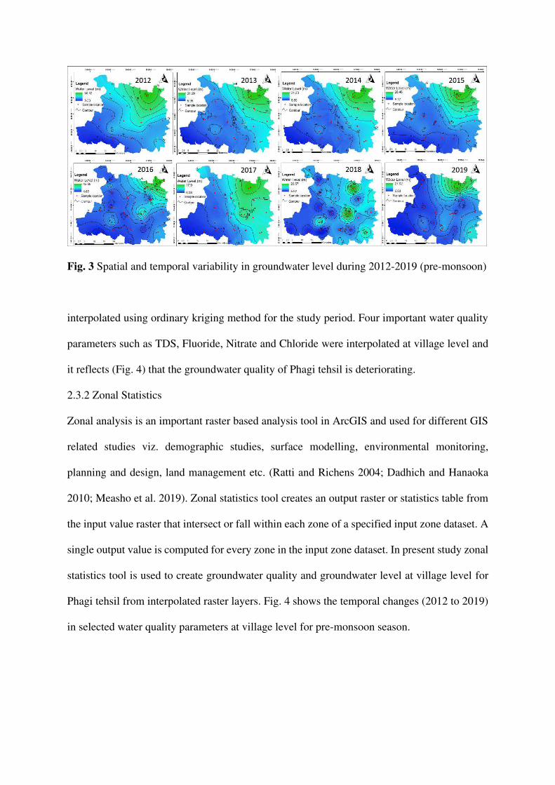
Fig. 3 Spatial and temporal variability in groundwater level during 2012-2019 (pre-monsoon)

interpolated using ordinary kriging method for the study period. Four important water quality

parameters such as TDS, Fluoride, Nitrate and Chloride were interpolated at village level and

it reflects (Fig. 4) that the groundwater quality of Phagi tehsil is deteriorating.

2.3.2 Zonal Statistics

Zonal analysis is an important raster based analysis tool in ArcGIS and used for different GIS

related studies viz. demographic studies, surface modelling, environmental monitoring,

planning and design, land management etc. (Ratti and Richens 2004; Dadhich and Hanaoka

2010; Measho et al. 2019). Zonal statistics tool creates an output raster or statistics table from

the input value raster that intersect or fall within each zone of a specified input zone dataset. A

single output value is computed for every zone in the input zone dataset. In present study zonal

statistics tool is used to create groundwater quality and groundwater level at village level for

Phagi tehsil from interpolated raster layers. Fig. 4 shows the temporal changes (2012 to 2019)

in selected water quality parameters at village level for pre-monsoon season.

Fig. 4 Temporal changes in groundwater quality (in mg/l) from 2012 to 2019

2.3.3 Time series forecasting

Time series analysis is an essential tool for better forecasts in hydrology studies (Bărbulescu

2016). In this study different time series forecasting techniques like Simple Exponential

Smoothing (SES), Holt's Trend Method (HTM) and ARIMA were applied using the statistical

programming language 'R' (Hyndman et al. 2017). Package in r language includes most of the

methods based on exponential smoothing or AutoRegressive Integrated Moving Average

(ARIMA) and related stochastic processes.

In SES method forecasts are produced using weighted averages of past observations,

with the weights decaying exponentially as the observations get older. In other words, higher

weights are given to the more recent observations and vice versa. The basic equation (Brown

and Robert G. 1956) is represented by ‘y’ beginning at time t = 0, and the output of the

exponential smoothing algorithm is written as ‘St’, which may be regarded as a best estimate

of what the next value of ‘y’ will be. Equation is expressed as: 𝑆𝑡 = αy𝑡−1 + (1– α)𝑆𝑡−1 (3)

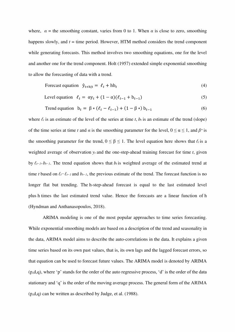
where, α = the smoothing constant, varies from 0 to 1. When α is close to zero, smoothing

happens slowly, and t = time period. However, HTM method considers the trend component

while generating forecasts. This method involves two smoothing equations, one for the level

and another one for the trend component. Holt (1957) extended simple exponential smoothing

to allow the forecasting of data with a trend.

Forecast equation ŷt+h|t = ℓ𝑡 + hb𝑡 (4)

Level equation ℓ𝑡 = αy𝑡 + (1 − α)(ℓ𝑡−1 + b𝑡−1) (5)

Trend equation b𝑡 = β ∗ (ℓ𝑡 − ℓ𝑡−1) + (1 − β ∗) b𝑡−1 (6)

where ℓt is an estimate of the level of the series at time t, bt is an estimate of the trend (slope)

of the time series at time t and α is the smoothing parameter for the level, 0 ≤ α ≤ 1, and β∗ is

the smoothing parameter for the trend, 0 ≤ β ≤ 1. The level equation here shows that ℓt is a

weighted average of observation yt and the one-step-ahead training forecast for time t, given

by ℓt−1+bt−1. The trend equation shows that bt is weighted average of the estimated trend at

time t based on ℓt−ℓt−1 and bt−1, the previous estimate of the trend. The forecast function is no

longer flat but trending. The h-step-ahead forecast is equal to the last estimated level

plus h times the last estimated trend value. Hence the forecasts are a linear function of h

(Hyndman and Anthanasopoulos, 2018).

ARIMA modeling is one of the most popular approaches to time series forecasting.

While exponential smoothing models are based on a description of the trend and seasonality in

the data, ARIMA model aims to describe the auto-correlations in the data. It explains a given

time series based on its own past values, that is, its own lags and the lagged forecast errors, so

that equation can be used to forecast future values. The ARIMA model is denoted by ARIMA

(p,d,q), where ‘p’ stands for the order of the auto regressive process, ‘d’ is the order of the data

stationary and ‘q’ is the order of the moving average process. The general form of the ARIMA

(p,d,q) can be written as described by Judge, et al. (1988).

∆𝑑𝑍𝑡 = C + [𝜙1 ∆𝑑 𝑍𝑡−1 + ⋯ + 𝜙𝑝 ∆𝑑 𝑍𝑡−𝑝 − (𝜙1𝑒𝑡−1 + ⋯ + 𝜙𝑝𝑒𝑡−𝑝) + 𝑒𝑡 (7)

where, ∆d denotes differencing of order d, i.e., ∆ Zt = Zt - Zt-1, ∆2 Zt-1 = ∆ Zt - ∆ Zt-1 and so on,

Zt-1 ----- Zt-p are past observations (lags), ‘C’ is a constant and 𝜙 1 -------- 𝜙 p are coefficient to

be estimated by auto regressive model. The auto regressive model of order ‘p’ denoted by AR

(P) and is written as

𝑍𝑡 = C + 𝜙1 𝑍𝑡−1 + 𝜙2 𝑍𝑡−2 + ⋯ + 𝜙𝑝 𝑍𝑡−𝑝 + 𝑒𝑡 (8)

where, et is a random variable with zero mean and constant variance. In the moving average

(MA) model, coefficient ‘F’ needs to be estimated. So MA model of order q can be written as:

𝑍𝑡 = 𝑒𝑡 − 𝜙1 e𝑡−1 − 𝜙2 e𝑡−2 − ⋯ − 𝜙𝑞 e𝑡−𝑞 (9)

The degree of the homogeneity (d) was determined on the basis of auto correlation function

(ACF) until ACF moves toward zero. Then after calculating‘d’ one need to examine a

stationary series Δd Zt, along with its auto correlation function and partial autocorrelation to

determine the values of p and q. Since a large number of factors affects the water level and

water quality and usually shows non linear relation with the variables; so traditional data

processing methods are not good enough (Xiang et al. 2006). Therefore, ANN approach has

advantages over semi-empirical models, since they require known input data set without any

assumptions and develops a mapping of the input and output variables, which can subsequently

be used to predict desired output as a function of suitable inputs (Schalkoff, 1992; Gardner and

Dorling, 1998). Multilayer Perceptron Neural Network (MLPNN) can approximate any

smooth, measurable function between input and output vectors by selecting a suitable set of

connecting weights and transfer functions (Singh et al. 2009). The ANN model has three or

more layers: the input layer where the data are introduced to the model and computation of the

weighted sum of the input is performed, the hidden layer or layers where data are processed,

and the output layer, where the results of ANN are produced. Each layer consists of one or

more basic element called a neuron or a node. The signal passing through the node is modified

by weights and transfer functions. Each node in the input and inner layers receives input values,

process it, and passes it to the next layer. This process is repeated until the output layer is

reached (Govindaraju 2000). The number of neurons in the input, hidden and output layers

depends on the problem, if number of hidden neurons is small, the network may not have

sufficient degrees of freedom to learn the process correctly however, if the number is too high,

the training will take longer time and the network may over-fit the data (Karunanithi et al.

1994).

For development of an optimized neural model, a wide range of models are developed,

trained and used for prediction of water quality parameters for the year 2019 based on data of

previous years. Predicted values of water quality parameters for year 2019 is then compared

with the observed values of 2019 using r2 and RMSE criterion discussed in next section. Based

on the performance evaluation criteria the optimized neural network with best performance is

then used for comparing it with other time series forecasting methods. In this study three

learning algorithms viz. networks using backpropagation, resilient backpropagation (RPROP)

with (Riedmiller 1994) or without weight backtracking or the modified globally convergent

version (GRPROP) by Anastasiadis et al. (2005) were used for testing and selection of best fit

ANN model towards predicting groundwater level in Phagi tehsil at village level.

Implementation of these algorithms in neuralnet r language package were utilized to

develop different models of neural networks. Fig. 5 shows the typical neural architecture with

Fig. 5 Typical neuralnet diagram showing relationship between inputs, neurons and output

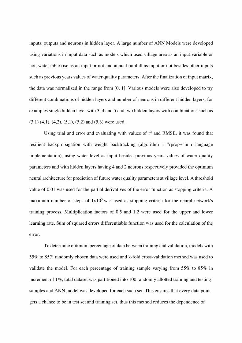
inputs, outputs and neurons in hidden layer. A large number of ANN Models were developed

using variations in input data such as models which used village area as an input variable or

not, water table rise as an input or not and annual rainfall as input or not besides other inputs

such as previous years values of water quality parameters. After the finalization of input matrix,

the data was normalized in the range from [0, 1]. Various models were also developed to try

different combinations of hidden layers and number of neurons in different hidden layers, for

examples single hidden layer with 3, 4 and 5 and two hidden layers with combinations such as

(3,1) (4,1), (4,2), (5,1), (5,2) and (5,3) were used.

Using trial and error and evaluating with values of r2 and RMSE, it was found that

resilient backpropagation with weight backtracking (algorithm = "rprop+"in r language

implementation), using water level as input besides previous years values of water quality

parameters and with hidden layers having 4 and 2 neurons respectively provided the optimum

neural architecture for prediction of future water quality parameters at village level. A threshold

value of 0.01 was used for the partial derivatives of the error function as stopping criteria. A

maximum number of steps of 1x105 was used as stopping criteria for the neural network's

training process. Multiplication factors of 0.5 and 1.2 were used for the upper and lower

learning rate. Sum of squared errors differentiable function was used for the calculation of the

error.

To determine optimum percentage of data between training and validation, models with

55% to 85% randomly chosen data were used and k-fold cross-validation method was used to

validate the model. For each percentage of training sample varying from 55% to 85% in

increment of 1%, total dataset was partitioned into 100 randomly allotted training and testing

samples and ANN model was developed for each such set. This ensures that every data point

gets a chance to be in test set and training set, thus this method reduces the dependence of

Fig. 6 Optimum % training using k fold cross-validation method

performance on test-training split and reduces the variance of performance metrics. Mean,

maximum, minimum and standard deviation of r2 for all 100 models were determined for each

% or training set and plotted as shown in Fig. 6. It can be seen that beyond 70%, standard

deviation is continuously rising indicating over training. Therefore 70% was used as optimum

training percentage.

2.3.4 Model Performance evaluation

The performance of the applied models can be assessed by several statistical error measures.

The root mean square error (RMSE), mean absolute error (MAE) and Nash-Sutcliffe

coefficient of efficiency (NSE) were used to provide an indication of goodness of fit between

the observed and predicted values. Expressions of these error parameters are given as follows:

𝑅𝑀𝑆𝐸 = √1𝑁 ∑(𝑋𝑂𝑏𝑠𝑒𝑟𝑣𝑒𝑑 − 𝑋𝑝𝑟𝑒𝑑𝑖𝑐𝑡𝑒𝑑)2 (10)

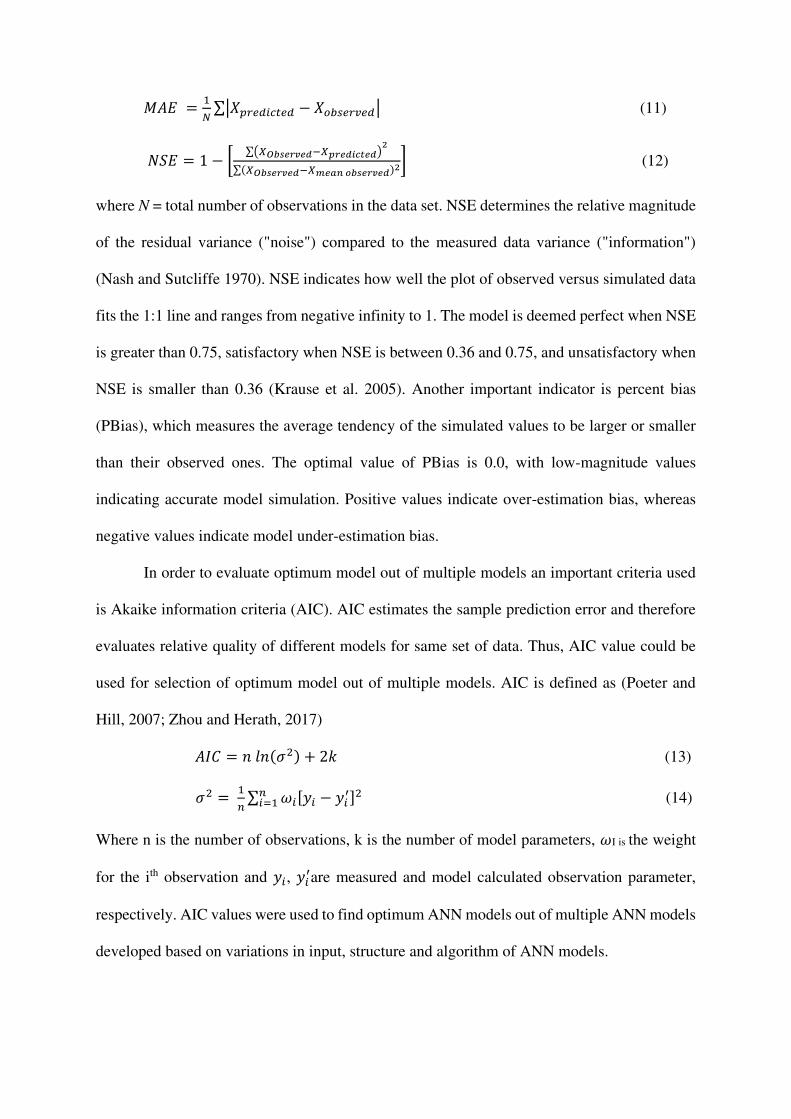
𝑀𝐴𝐸 = 1𝑁 ∑|𝑋𝑝𝑟𝑒𝑑𝑖𝑐𝑡𝑒𝑑 − 𝑋𝑜𝑏𝑠𝑒𝑟𝑣𝑒𝑑| (11)

𝑁𝑆𝐸 = 1 − [ ∑(𝑋𝑂𝑏𝑠𝑒𝑟𝑣𝑒𝑑−𝑋𝑝𝑟𝑒𝑑𝑖𝑐𝑡𝑒𝑑)2∑(𝑋𝑂𝑏𝑠𝑒𝑟𝑣𝑒𝑑−𝑋𝑚𝑒𝑎𝑛 𝑜𝑏𝑠𝑒𝑟𝑣𝑒𝑑)2] (12)

where N = total number of observations in the data set. NSE determines the relative magnitude

of the residual variance ("noise") compared to the measured data variance ("information")

(Nash and Sutcliffe 1970). NSE indicates how well the plot of observed versus simulated data

fits the 1:1 line and ranges from negative infinity to 1. The model is deemed perfect when NSE

is greater than 0.75, satisfactory when NSE is between 0.36 and 0.75, and unsatisfactory when

NSE is smaller than 0.36 (Krause et al. 2005). Another important indicator is percent bias

(PBias), which measures the average tendency of the simulated values to be larger or smaller

than their observed ones. The optimal value of PBias is 0.0, with low-magnitude values

indicating accurate model simulation. Positive values indicate over-estimation bias, whereas

negative values indicate model under-estimation bias.

In order to evaluate optimum model out of multiple models an important criteria used

is Akaike information criteria (AIC). AIC estimates the sample prediction error and therefore

evaluates relative quality of different models for same set of data. Thus, AIC value could be

used for selection of optimum model out of multiple models. AIC is defined as (Poeter and

Hill, 2007; Zhou and Herath, 2017) 𝐴𝐼𝐶 = 𝑛 𝑙𝑛(𝜎2) + 2𝑘 (13)

𝜎2 = 1𝑛 ∑ 𝜔𝑖[𝑦𝑖 − 𝑦𝑖′]2𝑛𝑖=1 (14)

Where n is the number of observations, k is the number of model parameters, 𝜔I is the weight

for the ith observation and 𝑦𝑖, 𝑦𝑖′are measured and model calculated observation parameter,

respectively. AIC values were used to find optimum ANN models out of multiple ANN models

developed based on variations in input, structure and algorithm of ANN models.

2.3.5 Water Quality Index (WQI) estimation

Water Quality Index (WQI) is a very useful and efficient method for assessing the overall

quality of water and to evaluate the suitability of the groundwater for drinking purposes (Abassi

1999; Asadi et al. 2007). For computing WQI, each of the four parameters has been assigned a

weight (wi) according to its relative importance in the overall quality of water for drinking

purposes (Ramakrishnaiah et al. 2009) and the relative weight (Wi) is computed from the

following equation:

𝑊𝑖 = 𝑤𝑖∑ 𝑤𝑖𝑛𝑖=1 (15)

where, Wi = relative weight, wi = weight of each parameter, and n = number of parameters.

Then quality rating scale (qi) is calculated for each parameter using following equation:

𝑞𝑖 = (𝐶𝑖𝑆𝑖) ∗ 100 (16)

where qi = quality rating for ith parameter, Ci = concentration of each chemical parameter in

each water sample in mg/l, and Si = drinking water standard for each chemical parameter in

mg/l according to the guidelines of World Health Organisation (WHO 2017). SI is first

determined for each chemical parameter, which is then used to determine the WQI as per the

following equation

𝑆𝐼𝑖 = 𝑊𝑖 ∗ 𝑞𝑖 (17)

𝑊𝑄𝐼 = ∑𝑆𝐼𝑖 (18)

SIi = sub index of ith parameter; qi = rating based on concentration of ith parameter, and n =

number of parameters. The computed WQI values are classified into five types, i.e. excellent

(WQI <50), good (WQI = 50–100), poor (WQI = 100–200), very poor (WQI = 200–300), and

water unsuitable for drinking (WQI >300).

Table 3 Groundwater Quality parameters, their WHO standards and assigned unit weights

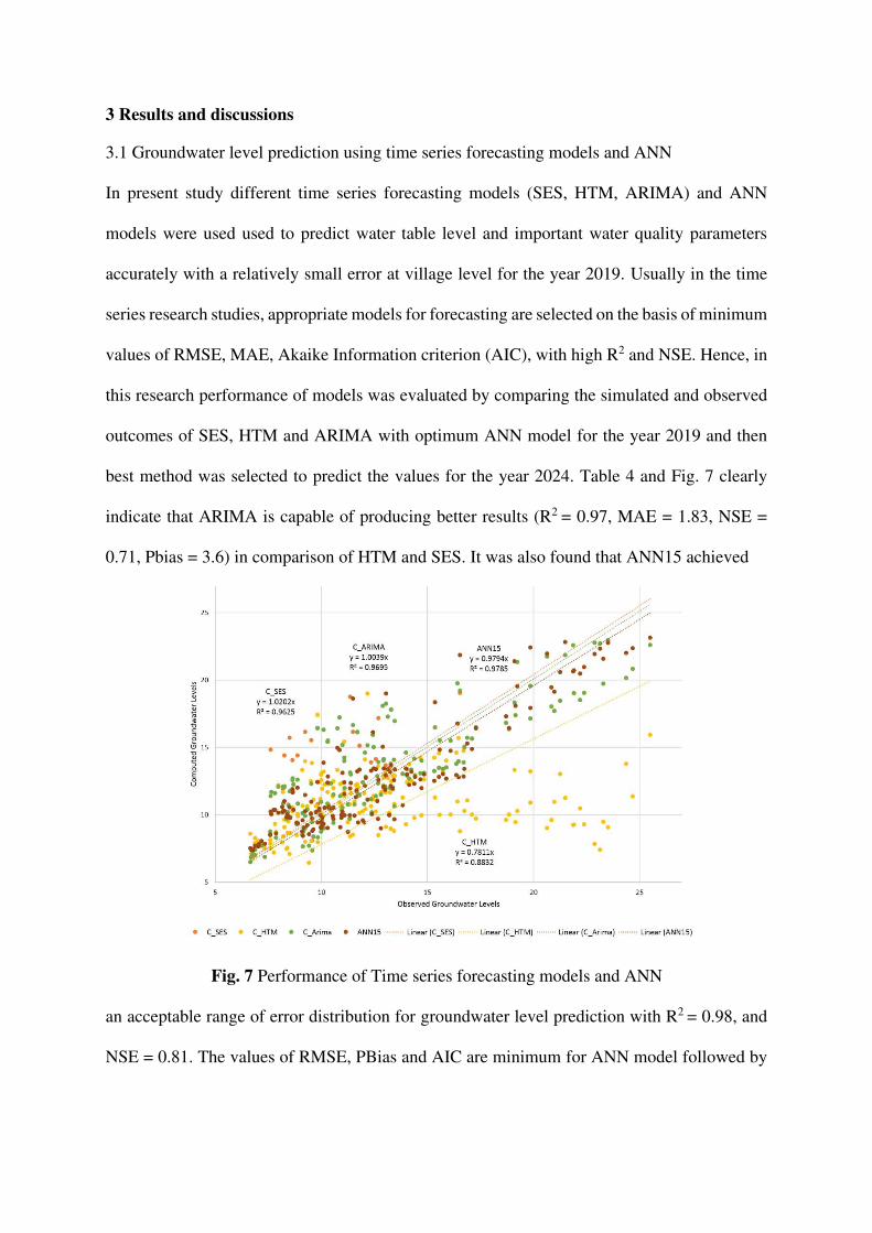
3 Results and discussions

3.1 Groundwater level prediction using time series forecasting models and ANN

In present study different time series forecasting models (SES, HTM, ARIMA) and ANN

models were used used to predict water table level and important water quality parameters

accurately with a relatively small error at village level for the year 2019. Usually in the time

series research studies, appropriate models for forecasting are selected on the basis of minimum

values of RMSE, MAE, Akaike Information criterion (AIC), with high R2 and NSE. Hence, in

this research performance of models was evaluated by comparing the simulated and observed

outcomes of SES, HTM and ARIMA with optimum ANN model for the year 2019 and then

best method was selected to predict the values for the year 2024. Table 4 and Fig. 7 clearly

indicate that ARIMA is capable of producing better results (R2 = 0.97, MAE = 1.83, NSE =

0.71, Pbias = 3.6) in comparison of HTM and SES. It was also found that ANN15 achieved

Fig. 7 Performance of Time series forecasting models and ANN

an acceptable range of error distribution for groundwater level prediction with R2 = 0.98, and

NSE = 0.81. The values of RMSE, PBias and AIC are minimum for ANN model followed by

ARIMA model. So this specifies that ANN model gives the best estimation of future values

and is used in further analysis.

Table 4 Comparison of Time series forecasting models with ANN

3.2 Groundwater level prediction using ANN models

Results (Fig. 8) infer that spatial distribution of observed and simulated groundwater level

values obtained from ANN15 is capable of close-fitting the hidden relationships in the time

series datasets. Therefore, ANN15 was used to forecast the groundwater level in the study area.

It is evident from spatial distribution (Fig. 8) that depth to water level varied upto 11mbgl in

Fig. 8 Observed, simulated and predicted mean values of depth to water level (mbgl) for

2019 and 2024 (pre-monsoon period)

south-western part of Phagi tehsil, however situation is alarming in northern villages of Phagi

tehsil as deeper water level were observed in Renwal Manjii (25.5mbgl), Beer Ramchandrapura

(24.67mbgl), Daloowala (24.37mbgl), Ganeshpura (23.52mbgl), Hari Rampura (23.29mbgl)

and Dabla Khurd (23.14mbgl) during pre-monsoon period of 2019. The water level predictions

for year 2024 indicate that in next five years some more villages will face significant drop in

groundwater level like Dabla Bujurg (23.6mbgl), Nihalpura@Miyan ka bas (23.16mbgl) and

Karwa (23.37mbgl).

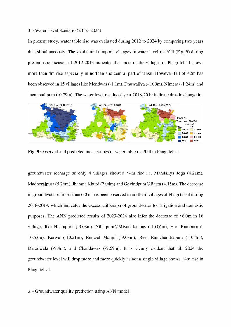
3.3 Water Level Scenario (2012- 2024)

In present study, water table rise was evaluated during 2012 to 2024 by comparing two years

data simultaneously. The spatial and temporal changes in water level rise/fall (Fig. 9) during

pre-monsoon season of 2012-2013 indicates that most of the villages of Phagi tehsil shows

more than 4m rise especially in northen and central part of tehsil. However fall of <2m has

been observed in 15 villages like Mendwas (-1.1m), Dhuwaliya (-1.09m), Nimera (-1.24m) and

Jagannathpura (-0.79m). The water level results of year 2018-2019 indicate drastic change in

Fig. 9 Observed and predicted mean values of water table rise/fall in Phagi tehsil

groundwater recharge as only 4 villages showed >4m rise i.e. Mandaliya Joga (4.21m),

Madhorajpura (5.76m), Jharana Khurd (7.04m) and Govindpura@Basra (4.15m). The decrease

in groundwater of more than 6.0 m has been observed in northern villages of Phagi tehsil during

2018-2019, which indicates the excess utilization of groundwater for irrigation and domestic

purposes. The ANN predicted results of 2023-2024 also infer the decrease of >6.0m in 16

villages like Heerapura (-9.08m), Nihalpura@Miyan ka bas (-10.06m), Hari Rampura (-

10.53m), Karwa (-10.21m), Renwal Manjii (-9.03m), Beer Ramchandrapura (-10.4m),

Daloowala (-9.4m), and Chandawas (-9.69m). It is clearly evident that till 2024 the

groundwater level will drop more and more quickly as not a single village shows >4m rise in

Phagi tehsil.

3.4 Groundwater quality prediction using ANN model

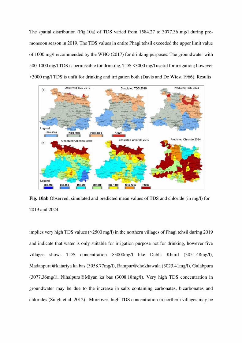
The spatial distribution (Fig.10a) of TDS varied from 1584.27 to 3077.36 mg/l during pre-

monsoon season in 2019. The TDS values in entire Phagi tehsil exceeded the upper limit value

of 1000 mg/l recommended by the WHO (2017) for drinking purposes. The groundwater with

500-1000 mg/l TDS is permissible for drinking, TDS <3000 mg/l useful for irrigation; however

>3000 mg/l TDS is unfit for drinking and irrigation both (Davis and De Wiest 1966). Results

Fig. 10ab Observed, simulated and predicted mean values of TDS and chloride (in mg/l) for

2019 and 2024

implies very high TDS values (>2500 mg/l) in the northern villages of Phagi tehsil during 2019

and indicate that water is only suitable for irrigation purpose not for drinking, however five

villages shows TDS concentration >3000mg/l like Dabla Khurd (3051.48mg/l),

Madanpura@katariya ka bas (3058.77mg/l), Rampur@chokhawala (3023.41mg/l), Gulabpura

(3077.36mg/l), Nihalpura@Miyan ka bas (3008.18mg/l). Very high TDS concentration in

groundwater may be due to the increase in salts containing carbonates, bicarbonates and

chlorides (Singh et al. 2012). Moreover, high TDS concentration in northern villages may be

attributed to the percolation of domestic sewage into the groundwater. The ANN predicted

values of TDS in pre-monsoon period of 2024 indicate that 14 villages of Phagi tehsil will

come under unfit groundwater category with very high concentration of TDS (>3000mg/l) in

villages like Ganeshpura (3218.62mg/l), Mohabbatpura (3261.72mg/l), Harsooliya

(3305.68mg/l), Mohanpura (3502.2mg/l), Jaichand ka bas (3277.06mg/l) and Manpur gate

(3228.43mg/l). High TDS is responsible for decrease in palatability and gastro-intestinal

irritation in humans (Sharma et al. 2017).

The chloride concentration (Fig. 10b) was found to be highly variable in the study area

ranging from 244.42 to 1922.31mg/l in 2019. The permissible limit of chloride is 250mg/l

(WHO 2017) which is observed in only one village i.e. Hanootiya Khurd (244.42mg/l). The

increase in chloride concentration is observed as index of pollution and indicates groundwater

contamination (Sarath Prasanth et al. 2012). Very high concentration of Chloride (>1250mg/l)

was observed in northern villages of the study area, this refers extreme groundwater

contamination in northern part of Phagi tehsil. The villages which exceeded the chloride

concentration (>1800mg/l) are Dabla Khurd (1893.42mg/l), Dabla Bujurg (1846.46mg/l),

Rampur@chokhawala (1846.79mg/l), Madanpura@katariya ka bas (1894.27mg/l),

Bheempura (1804.31mg/l), Koonchyawas (1810.03mg/l) and Gulabpura (1922.31mg/l). The

spatial distribution of ANNsimulated chloride values indicates almost same trend in 2019,

however in 2024, ANNpredicted values shows different situation of chloride concetration in

Phagi tehsil. Result implies that chloride concentration will range between 446.37mg/l and

1816.95mg/l in 2024 and refers that chloride concentration will be relatively lower in northern

villages of tehsil in comparison to eastern and western villages. The higher concentration of

chloride may affect the taste, indigestion and palatability in human (Bhunia et al. 2018).

The results of fluoride concentration (Fig.10c) reveal that fluoride ranged from 2.09 to

3.15mg/l in Phagi tehsil in 2019. The permissible limit for fluoride content is 1-1.5 mg/l (WHO

2017) and spatial distribution results indicate that entire Phagi tehsil is affected with high

concentration of fluoride. The main source of fluoride in groundwater is attributed to leaching

from fluoride rich rocks, semi-arid climate, long-term irrigation processes and long residence

Fig. 10cd Observed, simulated and predicted mean values of Fluoride and Nitrate (in mg/l)

for 2019 and 2024

time of groundwater (Srinivasamoorthy et al., 2008). High fluoride >1.2 mg/l results in dental

fluorosis however fluoride >2mg/l initiate mottling (Singh et al. 2012). The observed data

(2019) reveal that more than 3.0mg/l fluoride has been found in Khera Hanumanji (3.15mg/l),

Jharana Khurd (3.05mg/l), Madhorajpura (3.04mg/l), Mandaliya Joga (3.07mg/l) and

Mohabbatpura (3.02mg/l). However ANNsimulated data of 2019 reveal >3.0mg/l fluoride

concentration in 12 villages of Phagi tehsil (Fig. 7c). The ANN predicted fluoride concentration

for 2024 reveal that 47% of Phagi tehsil will be affected with >3.0mg/l fluoride especially in

eastern, central and northern villages of the study area. The adverse effects due to consumption

of fluoridated water are inevitably experienced by villagers in Phagi tehsil hence defluoridation

of drinking water is requisite in the study area.

The groundwater data of Phagi tehsil shows that Madanpura@katariya ka bas village

has maximum nitrate concentration (135.81mg/l) while Barh Ramchandrapura had minimum

(11.9 mg/l) in 2019. The observed and ANNsimulated results (Fig. 10d) for 2019 reveal that

nitrate content is higher than the maximum permissible limit recommended by WHO (WHO

2017) in northern and eastern villages of Phagi tehsil. Excess of nitrate is dangerous for infants

below six months age and when the concentration of nitrate ion exceeds 45-50 mg/l, it causes

methamoglobinemia in children (Sharma et. al. 2015). The higher content of nitrate (>120mg/l)

will occur in Ladana (135.59mg/l), Thala (133.76mg/l), Chittora (133.05mg/l), Bhojpura

(135.77mg/l), Jhadla (135.43mg/l), Barh bishanpura@Kagya (134.44mg/l), Sarswatipura

(134.42mg/l), Govindpura@Mandaliya (135.22mg/l) and Mukandpura (134.72mg/l). The

higher concentration of nitrate may be due to the sewage, organic matter and fertilizer from

agricultural runoff (Annapoorna and Janardhana 2015).

3.5 Water Quality Index

The Water quality index (WQI) was developed to evaluate the suitability of groundwater for

drinking purpose. The spatial and temporal changes (Fig. 11) during study period (2012 to

2024) indicates the degraded groundwater quality of Phagi tehsil. The WQI values for pre-

monsoon season of the year 2012 reveal that only one village i.e. Deonagar showed excellent

groundwater quality with the WQI 48.37, however very poor groundwater quality was

observed in Chandawas (WQI 201.71), Mohabbatpura (WQI 200.68), Ganeshpura (WQI

224.46), Beer Ramchandrapura (WQI 211.51), Renwal Manji (WQI 218.67), Basri Jogiyan

(WQI 214.15), Hari Rampura (WQI 200.69), Dabla Khurd (WQI 230.53) and Dabla Bujurg

(WQI 225.69).

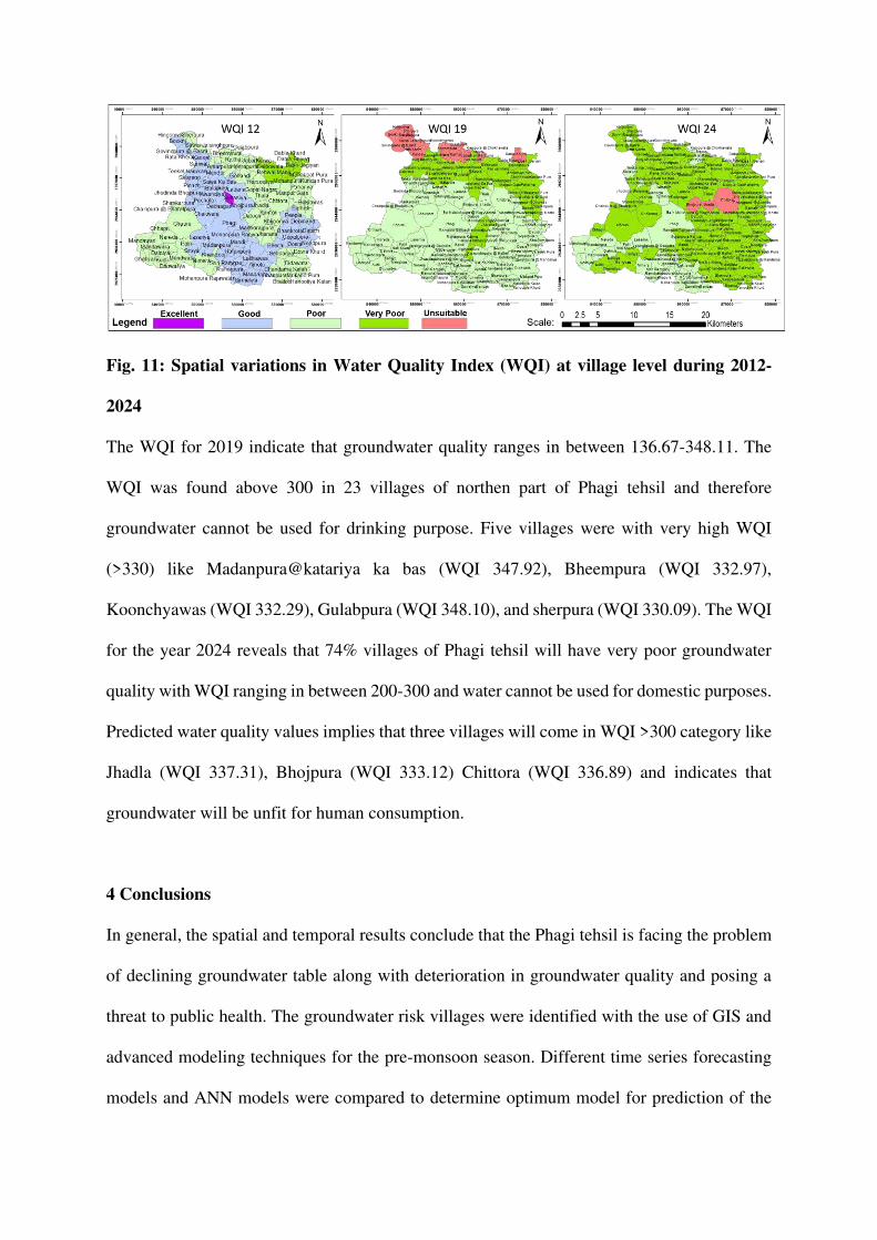
Fig. 11: Spatial variations in Water Quality Index (WQI) at village level during 2012-

2024

The WQI for 2019 indicate that groundwater quality ranges in between 136.67-348.11. The

WQI was found above 300 in 23 villages of northen part of Phagi tehsil and therefore

groundwater cannot be used for drinking purpose. Five villages were with very high WQI

(>330) like Madanpura@katariya ka bas (WQI 347.92), Bheempura (WQI 332.97),

Koonchyawas (WQI 332.29), Gulabpura (WQI 348.10), and sherpura (WQI 330.09). The WQI

for the year 2024 reveals that 74% villages of Phagi tehsil will have very poor groundwater

quality with WQI ranging in between 200-300 and water cannot be used for domestic purposes.

Predicted water quality values implies that three villages will come in WQI >300 category like

Jhadla (WQI 337.31), Bhojpura (WQI 333.12) Chittora (WQI 336.89) and indicates that

groundwater will be unfit for human consumption.

4 Conclusions

In general, the spatial and temporal results conclude that the Phagi tehsil is facing the problem

of declining groundwater table along with deterioration in groundwater quality and posing a

threat to public health. The groundwater risk villages were identified with the use of GIS and

advanced modeling techniques for the pre-monsoon season. Different time series forecasting

models and ANN models were compared to determine optimum model for prediction of the

future scenarios of groundwater quality and quantity in 171 villages of Phagi tehsil. Results of

the groundwater table shows the decline of >6.0 m especially in northern villages of Phagi

tehsil during the study period (2012-2024), which clearly indicates the excess utilization of

groundwater for irrigation and domestic purposes. Hence, it is suggested that reduce the

groundwater pumping and implement groundwater abstraction policy in high risk villages of

the study area. Apart from this, the percolation tanks or farm ponds may be constructed to

increase the natural recharge of rain water during monsoon period. Different groundwater

quality parameters like TDS, chloride and fluoride indicated that groundwater is not suitable

for drinking purpose in most of the villages of Phagi tehsil. The observed and ANNsimulated

results for 2019 reveal high nitrate content in north-eastern villages however, ANNpredicted

spatial distribution of nitrate for 2024 indicates that 58% villages of Phagi tehsil will exceed

the maximum permissible limit for drinking. The WQI specifies very poor to unsuitable

groundwater quality in 74% villages of the study area in 2024 indicating water cannot be used

for domestic purposes. Thus, the spatio-temporal maps suggests the necessity of groundwater

management with people’s participation for more effective implementation of a mitigation

strategy in Phagi tehsil at village level.

Acknowledgment

Authors acknowledge Department of Science & Technology, Government of India for financial

support vide reference number DST/WOS-B/2018/1575/ETD/Ankita under Women Scientist

Scheme (WOS-B) to carry out this research work.

Declarations

Ethical Approval: Not applicable

Consent to Participate: This manuscript in part or in full has not been submitted or

published anywhere. The manuscript will not be submitted elsewhere until the

editorial/review process is completed.

Consent to Publish: Hereby all authors agree for publication of this manuscript in WARM

Authors Contributions: All authors contributed to this manuscript

1. Dr. Ankita Pran Dadhich: Conceived and designed the analysis; performed analysis; wrote

the manuscript

2. Dr. Rohit Goyal: Contributed in analysis tools and provided inputs in writing manuscript

3. Dr. Pran Nath Dadhich: Conceived & Collected data and provided inputs in writing

manuscript

Funding: Department of Science & Technology, Government of India for financial support

vide reference number DST/WOS-B/2018/1575/ETD/Ankita under Women Scientist Scheme

(WOS-B) to carry out this research work.

Competing Interests: Not applicable

Availability of data and materials: Will be provided as per the requirement of Editor/

Reviewer

References

Abassi SA (1999) Water Quality Indices, State-of-the art. J.IPHE. No.1.

Ahmadi S, Sedghamiz A (2007) Geostatistical analysis of spatial and temporal variations of

groundwater level. Environ Monit Assess 129(1–3):277–294

Anastasiadisa AD, Magoulasa GD, Vrahatis MN (2005) New globally convergent training

scheme based on the resilient propagation algorithm. Neurocomputing 64:253-270

Annapoorna H, Janardhana MR (2015) Assessment of Groundwater Quality for Drinking

Purpose in Rural Areas Surrounding a Defunct Copper Mine. Aquat Procedia 4:685 – 692

Asadi SS, Vuppala P, Reddy MA (2007) Remote Sensing and GIS Techniques for Evaluation

of Groundwater Quality in Municipal Corporation of Hyderabad (Zone-V), India. Int. J Environ

Res Public Health 4(1): 45-52

Ay M, Kisi O (2012) Modeling of dissolved oxygen concentration using different neural

network techniques in Foundation Creek, El Paso County, Colorado. J Environ Eng 138:654–

662

Bărbulescu A (2016) Studies on Time Series Applications in Environmental Sciences. Springer

International Publishing, Cham, Switzerland. https://doi.org/10.1007/978-3-319-30436-6

Bhunia GS, Keshavarzi A, Shit PK, Omran ESE, Bagherzadeh A (2018) Evaluation of

groundwater quality and its suitability for drinking and irrigation using GIS and geostatistics

techniques in semiarid region of Neyshabur, Iran. Appl Water Sci 8:168

Brown, Robert G (1956). Exponential Smoothing for Predicting Demand. Cambridge,

Massachusetts: Arthur D. Little Inc. p. 15.

Central Ground Water Board (2017) Report on aquifer mapping and ground water

management, Jaipur District. Ministry of Water Resources, River Development & Ganga

Rejuvenation, Western Region Jaipur, Rajasthan Government of India.

Charulatha G, Srinivasalu S, Maheswari OU, Venugopal T, Giridharan L (2017). Evaluation

of ground water quality contaminants using linear regression and artificial neural network

models. Arab J Geosci 10:128

Chenini I, Ben MA (2010) Groundwater recharge study in arid region: an approach using GIS

techniques and numerical modeling. Comput Geosci 36(6):801–817

Csábrági A, Molnár S, Tanos P, Kovács J (2017) Application of artificial neural networks to

the forecasting of dissolved oxygen content in the Hungarian section of the river Danube. Ecol

Eng 100:63–72

Dadhich PN, Hanaoka S (2010) Remote sensing, GIS and Markov’s method for land use

change detection and prediction of Jaipur District. J Geomatics 4(1) 9-15

Davis SN, De Wiest RJM (1966). Hydrogeology, vol 463. Wiley, New York.

Gardner MW, Dorling SR (1998) Artificial neural networks (the multilayer perceptron)—a

review of applications in the atmospheric sciences. Atm Environ 32(14–15):2627-2636

Gautam SK, Tziritis E, Singh SK, Tripathi JK, Singh AK (2018) Environmental monitoring of

water resources with the use of PoS index: a case study from Subarnarekha River basin, India.

Environ Earth Sci 77:70

Gharbia AS, Gharbia SS, Abushbak T, Wafi H, Aish A, Zelenakova M, Pilla F (2016)

Groundwater Quality Evaluation Using GIS Based Geostatistical Algorithms. J Geosci Environ

Prot 4(2):89-103

Ghazavi R, Vali AB, Eslamian S (2012) Impact of Flood Spreading on Groundwater Level

Variation and Groundwater Quality in an Arid Environment. Water Resour Manage (2012)

26:1651–1663

Govindaraju RS (2000) Artificial neural network in hydrology. II: hydrologic application,

ASCE task committee application of artificial neural networks in hydrology.J Hydrol Eng

5:124–137

Holt CC (1957) Forecasting Trends and Seasonals by Exponentially Weighted

Averages, Carnegie Institute of Technology, Pittsburgh Office of Naval Research

memorandum no. 52.

Hyndman RJ, Athanasopoulos G (2018) Forecasting: principles and practice. 2nd

edition, OTexts: Melbourne, Australia. OTexts.com/fpp2.

Hyndman RJ, O'Hara-Wild M, Bergmeir C, Razbash S, Wang E (2017) Forecast: Forecasting

functions for time series and linear models. R package version 8.2.

https://CRAN.Rproject.org/package=forecast

Jolly ID, McEwan KL, Holland KL (2008) A review of groundwater-surface water interactions

in arid/semi-arid wetlands and the consequences of salinity for wetland ecology. Ecohydrology

1:43–58

Journel AG, (1989) In: Fundamentals of Geostatistics in Five Lessons, Short Course in

Geology, vol. 8. American Geophysical Union.

Judge GG, Hill RC, William EG, Helmut I (1988) Introduction to the Theory and Practice of

Econometrics. 2nd ed., John Wiley and Son, INC. New York, Toronto, Singapore

Karunanithi N, GrenneyWJ, Whitley D, Bovee K (1994) Neural networks for river flow

prediction. ASCE J Comput Civil Eng 8:210–220.

Krause P, Boyle DP, Base F (2005) Comparison of different efficiency criteria for hydrological

model assessment. Adv Geosci 5(1):89-97

Kumar VS, Amarender B, Dhakate R, Sankaran S, Kumar KR (2016) Assessment of

groundwater quality for drinking and irrigation use in shallow hard rock aquifer of

Pudunagaram, Palakkad District Kerala. Appl Water Sci 6:149–167

Marsily D, (1986). Quantitative Hydrogeology. Academic Press.

Measho S, Chen B, Trisurat Y, Pellikka P, Guo L, Arunyawat S, Tuankrua V, Ogbazghi W,

Yemane T (2019) Spatio-Temporal Analysis of Vegetation Dynamics as a Response to Climate

Variability and Drought Patterns in the Semiarid Region, Eritrea. Remote Sens 11:724

Minville M, Krau S, Brissette F, Leconte R (2010) Behaviour and performance of a water

resource system in Québec (Canada) under adapted operating policies in a climate change

context. Water Resour Manag 24:1333–1352

Mohanty, S., Jha, M. K., Kumar, A., & Sudheer, K. P. (2010). Artificial neural network

modeling for groundwater level forecasting in a river island of eastern India. Water Resour

Manage 24:1845–1865

Nas B, Berktay A (2010) Groundwater quality mapping in urban groundwater using GIS.

Environ Monit Assess 160:215–227

Nash JE, Sutcliffe JV (1970) River flow forecasting through conceptual models. Part I—a

discussion of principles. J Hydrology 10:282–290

Nayak TR, Gupta SK, Galkate R (2015) GIS Based Mapping of Groundwater Fluctuations in

Bina Basin Aquat Procedia 4:1469 – 1476

Poeter EP, Hill MC (2007) MMA, a Computer Code for Multi-Model Analysis: U.S.

Geological Survey Techniques and Methods 6eE3, Boulder, Colo, 113 p.

Ramakrishnaiah CR, Sadashivaiah C, Ranganna G (2009) Assessment of water quality index

for the groundwater in Tumkar Taluk, Karnataka State, India. E-J Chem 6(2):523–530

Ratti C, Richens P (2004) Raster Analysis of Urban Form. Environ Plann B Plann Des 31(2):

297-309

Rawat KS, Singh SK, Gautam SK (2018) Assessment of groundwater quality for irrigation use:

a peninsular case study. Appl Water Sci 8:233

Riedmiller M (1994) Rprop - Description and Implementation Details. Technical Report.

University of Karlsruhe.

Sarath Prasanth SV, Magesh NS, Jitheshlal KV, Chandrasekar N, Gangadhar K (2012)

Evaluation of groundwater quality and its suitability for drinking and agricultural use in the

coastal stretch of Alappuzha District, Kerala, India. Appl Water Sci 2:165–175

Schalkoff R (1992) Pattern Recognition: Statistical, Structural and Neural Approaches, Wiley,

New York, 364 p.

Sharma DA, Rishi MS, Keesari T (2017) Evaluation of groundwater quality and suitability for

irrigation and drinking purposes in southwest Punjab, India using hydrochemical approach.

Appl Water Sci 7:3137-3150

Sharma SK, Sharma U, Chandel CPS (2015) Qualitative aspects of Ground water for Drinking

purpose of Phagi Block of Jaipur District (Rajasthan). Ascent Int J Res Analysis 2(2): 57.1-

57.9

Singh K, Basant A, Malik A, Jain G (2009) Artificial neural network modeling ofthe river

water quality—a case study. Ecol Modell 220:888–895

Singh P, Fahmi N, Singh VP, Singh RV (2012) Studies on Ground Water Fluoride Content and

Water quality in Phagi Tehsil of Jaipur District. Int J Chem Environ Pharm Res 3(3): 219-224

Singh SK, Srivastava PK, Pandey AC, Gautam SK (2013) Integrated assessment of

groundwater influenced by a confluence river system: concurrence with remote sensing and

geochemical modelling. Water Resour Manag 27(12):4291–4313

Srinivasamoorthy K, Chidambaram S, Vasanthavigar M (2008) Geochemistry of fluorides in

groundwater, Salem District, Tamilnadu, India. J Env Hydrol 1:16-25

Srivastava PK, Gupta M, Mukherjee S (2012) Spatial distribution of pollutants in groundwater

of a tropical area of India using remote sensing and GIS. Appl Geomatics 4:21–32

Sunayana, Kalawapudi K, Dube O, Sharma R (2019) Use of neural networks and spatial

interpolation to predict groundwater quality.Environ Dev Sustain 22: 2801-2816

Ta’any RA, Tahboub AB, Saffarini GA (2009) Geostatistical analysis of spatiotemporal

variability of groundwater level fluctuations in Amman–Zarqa basin, Jordan: a case study.

Environ Geol 57:525–535

Verma DK, Bhunia GS, Shit PK, Kumar S, Mandal J, Padbhushan R (2017) Spatial variability

of groundwater quality of Sabour block, Bhagalpur district (Bihar, India). Appl Water Sci

7:1997-2008

WHO. (2017). Guidelines for drinking water quality: training pack (4th ed.). Geneva,

Switzerland: Incorporating The First Addendum

Xiang SL, Liu ZM, Ma LP (2006) Study of multivariate linear regression analysis model for

ground water quality prediction. Guizhou Sci 24(1):60–62

Yesilnacar MI, Sahinkaya E, Naz M, Ozkaya B (2008) Neural network prediction of nitrate in

groundwater of Harran Plain, Turkey. Environ Geology 56(1):19–25

Zhou Y, Herath HMPSD (2017) Evaluation of alternative conceptual models for groundwater

modelling, Geosci Front 8(3):437-443

Figures

Figure 1

Location and Hydrogeology of the study area

Figure 2

(a) Variations in annual rainfall (2005-2019) source: Central Ground Water Board, Jaipur (b) Samplinglocations in Phagi Tehsil

Figure 3

Spatial and temporal variability in groundwater level during 2012-2019 (pre-monsoon)

Figure 4

Temporal changes in groundwater quality (in mg/l) from 2012 to 2019

Figure 5

Typical neuralnet diagram showing relationship between inputs, neurons and output

Figure 6

Optimum % training using k fold cross-validation method

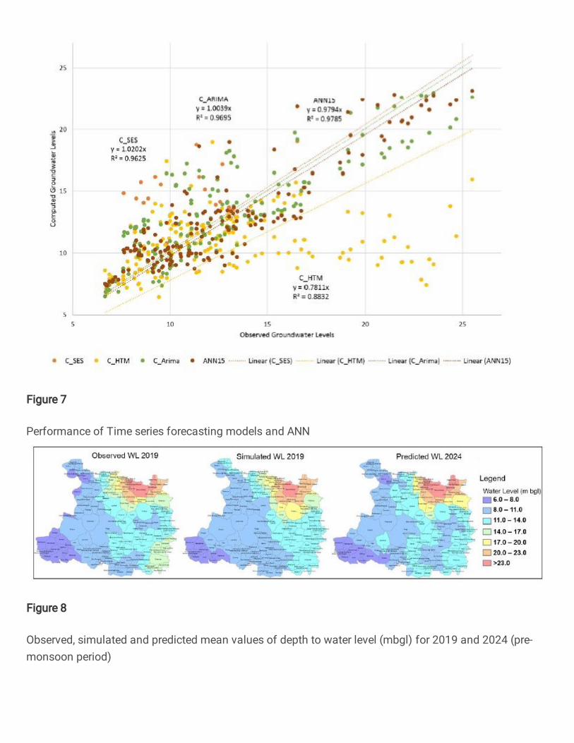
Figure 7

Performance of Time series forecasting models and ANN

Figure 8

Observed, simulated and predicted mean values of depth to water level (mbgl) for 2019 and 2024 (pre-monsoon period)

Figure 9

Observed and predicted mean values of water table rise/fall in Phagi tehsil

Figure 10

(a) and (b): Observed, simulated and predicted mean values of TDS and chloride (in mg/l) for 2019 and2024. (c) and (d): Observed, simulated and predicted mean values of Fluoride and Nitrate (in mg/l) for2019 and 2024

Figure 11

Spatial variations in Water Quality Index (WQI) at village level during 2012-2024