Embed Size (px)
Citation preview

Assessing vulnerability due to sea-level rise in Maui,Hawai‘i using LiDAR remote sensing and GIS
Hannah M. Cooper & Qi Chen & Charles H. Fletcher & Matthew M. Barbee
Received: 19 September 2011 /Accepted: 22 May 2012# Springer Science+Business Media B.V. 2012
Abstract Sea-level rise (SLR) threatens islands and coastal communities due to vulnerableinfrastructure and populations concentrated in low-lying areas. LiDAR (Light Detection andRanging) data were used to produce high-resolution DEMs (Digital Elevation Model) forKahului and Lahaina, Maui, to assess the potential impacts of future SLR. Two existingLiDAR datasets from USACE (U.S. Army Corps of Engineers) and NOAA (NationalOceanic and Atmospheric Administration) were compared and calibrated using the KahuluiHarbor tide station. Using tidal benchmarks is a valuable approach for referencing LiDAR inareas lacking an established vertical datum, such as in Hawai‘i and other Pacific Islands.Exploratory analysis of the USACE LiDAR ground returns (point data classified as groundafter the removal of vegetation and buildings) indicated that another round of filtering couldreduce commission errors. Two SLR scenarios of 0.75 (best-case) to 1.9 m (worst-case)(Vermeer and Rahmstorf Proc Natl Acad Sci 106:21527–21532, 2009) were considered, andthe DEMs were used to identify areas vulnerable to flooding. Our results indicate that if noadaptive strategies are taken, a loss ranging from $18.7 million under the best-case SLRscenario to $296 million under the worst-case SLR scenario for Hydrologically Connected(HC; marine inundation) and Hydrologically Disconnected (HD; drainage problems due to ahigher water table) areas combined is possible for Kahului; a loss ranging from $57.5 millionunder the best-case SLR scenario to $394 million under the worst-case SLR scenario for HC
Climatic ChangeDOI 10.1007/s10584-012-0510-9
H. M. Cooper (*) : Q. ChenDepartment of Geography, University of Hawai‘i, 2424 Maile Way, Honolulu, HI 96822, USAe-mail: [email protected]
Q. Chene-mail: [email protected]
H. M. Cooper : C. H. Fletcher :M. M. BarbeeDepartment of Geology and Geophysics, School of Ocean and Earth Science and Technology, Universityof Hawai‘i, 1680 East West Road, Honolulu, HI 96822, USA
C. H. Fletchere-mail: [email protected]
M. M. Barbeee-mail: [email protected]

and HD areas combined is possible for Lahaina towards the end of the century. This losswould be attributable to inundation between 0.55 km2 to 2.13 km2 of area for Kahului, and0.04 km2 to 0.37 km2 of area for Lahaina.
1 Introduction
Accelerated sea-level rise (SLR) due to climate change threatens human communities livingnear the coast worldwide. It is estimated that about half of the world’s population lives incoastal areas (GOF 2011). According to the U.S. Census Bureau (2011), about half of theU.S. population lives in coastal counties. As population and land development continue togrow in low-lying coastal communities, the impacts of climate change will become moreapparent (CCSP 2009).
According to the Intergovernmental Panel on Climate Change (IPCC 2007), globalsea level may rise 0.18 to 0.59 m by the end of the 21st century. Thermal expansionof ocean water and melting of land-based ice are the two major contributors to globalSLR. However, the IPCC (2007) estimates are understood to underestimate globalSLR by 2100 because they exclude important contributions due to some forms of icemelt (Fletcher 2009).
Vermeer and Rahmstorf (2009) modeled that global sea level may rise 0.75 to1.9 m by the end of the 21st century. To estimate the overall sea level responseincluding ice melt, they developed a semi-empirical model based on observed globalsea level and temperature data from 1880–2000 to find that the rate of SLR is closelyconnected to global temperature. The Vermeer and Rahmstorf model was applied tothe IPCC global temperature estimates for 1880–2100; they found that late in the 21stcentury, thermal expansion declines as ice melt begins to increase. As their modelshows that ice melt will become more important later in the 21st century, Vermeerand Rahmstorf (2009) estimates of global SLR by 2100 are significantly different thanIPCC (2007) estimates.
Vulnerability to SLR is a function of a community’s potential exposure, sensitivity,and adaptive capacity (IPCC 2007). The major impacts of SLR on natural systemsinclude: inundation, wetland loss, erosion, saltwater intrusion, areas of less drainageand rising water tables; as a result, this may lead to adverse socioeconomic impactson coastal populations/infrastructure, ports/industry, recreational activities and tourism(Nicholls 2011). Vulnerability may be influenced by social factors such as population,physical factors such as infrastructure (Wu et al. 2002), and economic factors such asland and building value. Socioeconomic factors such as these determine a coastalcommunity’s vulnerability to SLR (McLeod et al. 2010). One way to assess vulner-ability is to map low-lying areas utilizing a DEM (Digital Elevation Model). DEMsare critical to mapping low-lying lands and to identifying communities, infrastructure,and coastal habitats vulnerable to inundation due to SLR.
Gesch (2009) compared DEMs used in previous SLR vulnerability assessmentssuch as U.S. Geological Survey (USGS) global 30-arc second GTOPO30 (∼1 kmhorizontal resolution), Shuttle Radar Topographic Mission (SRTM) (∼90 m horizontalresolution), and National Elevation Dataset (NED) (30 m horizontal resolution) withLight Detection and Ranging (LiDAR) (3 m horizontal resolution) to determine thatLiDAR DEMs provide improvements to mapping vulnerable lands due to their highhorizontal resolution and vertical accuracy. Zhang (2011) examined the effect ofvertical accuracy of DEMs comparing a 30 m LiDAR DEM with a 30 m USGS
Climatic Change

DEM to determine that the high vertical accuracy of LiDAR DEMs is essential toestimating land area, population and property vulnerable to SLR. Zhang (2011) alsoexamined the effect of horizontal resolution on identifying individual propertiesvulnerable to SLR by comparing 30 and 5 m LiDAR DEMs to determine that LiDARDEMs ≤5 m horizontal resolution are necessary. Poulter and Halpin (2008) investi-gated the effects of horizontal resolution and hydrologic connectivity using 15 and6 m LiDAR DEMs to determine that the rules for hydrologic connectivity interactedwith horizontal resolution most critically at SLR scenarios <0.4 m.
In Hawai‘i, high-resolution LiDAR DEMs are useful to assess the impacts of SLR.Hawai‘i is the only U.S. state that consists exclusively of islands, where socioeco-nomic activity is concentrated in low-lying coastal communities. Clearly, acceleratedSLR may be one of the most significant impacts of climate change in the region.However, the implications of climate change on the Hawai‘i archipelago is not wellunderstood. There is an urgent need to improve community resiliency to marinehazards, and coastal planning in Hawai‘i currently does not require SLR vulnerabilityassessments to help planners identify the lowest-lying lands and the critical infrastruc-ture that is on them (Fletcher et al. 2010).
This study examines the vulnerability due to inundation of Kahului and Lahaina, Maui,using the SLR estimates by Vermeer and Rahmstorf (2009). Due to the uncertainty in theirestimates, a scenario-building approach (NOAA 2001) is utilized where the +0.75 mestimate is used as a best-case SLR scenario, and the +1.9 m estimate is used as a worst-case SLR scenario. The purpose of this study is to use LiDAR DEMs to map low-lying landsvulnerable to SLR combined with spatial analysis to identify coastal habitats, roads, land andbuilding values that are likely to experience adverse impacts.
2 Study area and data
2.1 Study area
The study area includes two communities with the most socioeconomic activity onMaui Island: Kahului and Lahaina (Fig. 1). Kahului is the largest community on theisland with a Census 2010 population of nearly 26,000. The study area coveringKahului is ∼8.9 km2. Kahului is located on the north shore of a low-relief isthmus ona coastal plain between the dormant Haleakalā volcano to the east, and the extinctWest Maui Volcano. Kahului is the industrial center of the island and the location ofKahului Harbor, Maui’s commercial deep-draft harbor; and Kahului Airport, Maui’smain airport that accommodates inter-island and mainland flights. Just inland to theHarbor sits the wetlands of Kanaha Pond, a designated National Natural Landmarkand wildlife refuge for endangered Hawaiian bird species such as the ae‘o (Hawaiianstilt), and the ‘alae ke‘oke‘o (Hawaiian coot). Heavy vegetation surrounds KanahaPond and the shoreline just east of the wildlife refuge at Kanaha Beach Park.
Lahaina is an historic port town and largest community located on the shore of West Mauiwith a Census 2010 population of nearly 11,700. The study area covering Lahainais ∼4.9 km2. As the second largest tourism destination of the Hawaiian Islands followingWaikiki, visitors account for a much higher population around 40,000 during peak travelseason. Lahaina’s shoreline consists of critical infrastructure such as the only highway thatleads to Lahaina, the Hono a Pi‘ilani Highway (Route 30), coastal roads, and the LahainaHarbor.
Climatic Change

2.2 Airborne LiDAR data
Two separate existing LiDAR datasets were used for Kahului and Lahaina, respec-tively. The data for Kahului were collected by the Joint Airborne LiDAR BathymetryTechnical Center of Expertise (JALBTCX) for the U.S. Army Corps of Engineers(USACE) in January through February of 2007 using the Compact HydrographicAirborne Rapid Total Survey (CHARTS) system equipped with the OptechSHOALS-3000 sensor. The flight altitude varied from 300 to 1,200 m above groundlevel. The metadata reports the average laser point spacing as 1.3 m, and the verticalroot mean square error (RMSE) as better than ±0.20 m. The Kahului data are calledUSACE LiDAR hereinafter. The data for Lahaina were collected by EarthDataAviation for the National Oceanic and Atmospheric Administration (NOAA) in Marchof 2005 during Mean Lower Low Water (MLLW) tides using the Leica GeosystemsALS-40. The flight altitude was ∼800 m above mean ground level. The metadatareports the average laser point spacing as 2 m, the RMSE as ±0.162 m, and thevertical accuracy as ±0.318 m at the 95 % confidence level. The Lahaina data arecalled NOAA LiDAR hereinafter. Both USACE and NOAA LiDAR data were cap-tured by discrete-return, scanning airborne laser altimeters with a pulse rate of20,000 Hz.
Orthometric elevations were derived from the Geodetic Reference System of 1980(GRS80) ellipsoid elevations using the National Geodetic Survey (NGS) GEOID03 modelfor USACE, and the NGS GEOID09 model for NOAA. These elevations were adjusted tothe Local Tidal Datum of Mean Sea Level (MSL) and are in meters. However, it is unclear towhich MSL tidal datum epoch the USACE and NOAA LiDAR are vertically referenced.The horizontal coordinates for the two data are relative to the North American Datum of1983 (NAD83) and are in meters. The two data were received as classified ground returns inxyz format from the NOAA Coastal Services Center (CSC).
Fig. 1 Study areas of Kahului and Lahaina on Maui Island
Climatic Change

3 Methods
3.1 LiDAR data filtering and DEM generation
The quality of a LiDAR DEM is highly dependent on the average point spacing and the post-processing software used to filter the raw LiDAR 3-dimensional (3-D) point cloud, a set ofpoints defined by xyz in a coordinate system. The data service providers for the USACE andNOAA LiDAR point data used proprietary procedures and software when filtering theLiDAR point cloud into classified ground returns. For this reason, an exploratory analysisof the USACE and NOAA ground returns was conducted to determine the effect of filteringmethods on inundation analysis. DEMs of 2 m horizontal spatial resolution were generatedfrom the two datasets using Toolbox for LiDAR Data Filtering and Forest Studies (Tiffs)software (Chen 2007). The 2 m cell size was chosen due to the average point spacing of thetwo data. The xyz files were also converted to the shapefile format so that the DEMs andLiDAR point shapefiles could be overlaid in 3-D using ESRI’s ArcScene and visuallycompared with 2005 and 2007 aerial photos. This allowed for identification of any remain-ing vegetation or buildings that were not removed when the LiDAR point cloud wasclassified into ground and non-ground returns (e.g. vegetation and buildings).
Exploratory analysis of the NOAA ground returns overlaid with 2005 aerial photosdemonstrated a lack of ground returns near buildings and vegetation. Since filtering theLiDAR point data is intended to remove vegetation and infrastructure, this is likely a causeof over-classification of the points as non-ground returns. This could not be further exam-ined because the non-ground returns were not available for download from NOAA CSC toinclude in the exploratory analysis. It could not be determined how the filtering methodsused for the NOAA data impact the DEM and inundation analysis for Lahaina.
Exploratory analysis of the USACE ground returns overlaid with 2007 aerial photosfound vegetation along the coastline at Kanaha Beach Park and near Kanaha pond, whichcreated topographic anomalies in the DEM. This is likely a cause of poor penetration of theLiDAR through thick canopy and misclassification of vegetation as ground returns. TheTiffs software uses an automatic grid-based filtering or morphological method (Chen et al.2007), which was used to re-classify ground returns from the USACE data. This was donewith caution to not over-classify vegetated areas that would leave a lower point density, suchas in the NOAA data. After the points were re-classified, the ground returns were used to re-generate a refined 2 m USACE DEM.
3.2 Assessing vertical accuracy using tidal benchmarks
The standard for determining the quality of LiDAR data for the purpose of generating aDEM is to relate the data to a vertical datum (Maune 2007; Liu 2011). It is unclear whetherthe USACE and NOAA LiDAR are vertically referenced to the Local Tidal Datum of MSLfor the recent 1983–2001 epoch. Therefore, this study used tidal benchmarks to assess theUSACE LiDAR data and to determine if a calibration was needed. The USACE LiDAR wasthen used to determine if the NOAA LiDAR required calibration, due to the deficiency oftidal benchmarks in West Maui.
A particular order and class defined by the NGS classify the vertical accuracy of the tidalbenchmarks, where more information on leveling can be found at http://www.ngs.noaa.gov/heightmod/Leveling/requirements.html. The tidal benchmarks 161 5680 A and C TIDAL areclassified as third-order (the least accurate) and the seven remaining tidal benchmarks areclassified as first-order, class I (most accurate). The tidal benchmark elevations were
Climatic Change

compared with elevations derived from the USACE LiDAR data to calculate the meandifference, RMSE and the linear error (L.E.Z) at 95 % confidence. A standard t-test was usedto inspect the difference between the tidal benchmark elevations and USACE LiDARelevations, and the difference between the average elevations of the USACE and NOAALiDAR point data in Northwest Maui where the two LiDAR datasets overlap to determine ifa calibration was needed.
The LiDAR data filtering methods used may also affect the vertical accuracy assessmentof the data because ground returns may have been misclassified (Liu 2011). The tidalbenchmarks are located in flat and non-vegetated terrain, yet the LiDAR filtering processmay have incorrectly classified non-ground returns as ground returns in the LiDAR pointdata covering the tidal benchmarks. In order to visualize the accuracy of the LiDAR pointdata, both the LiDAR point data and tidal benchmark point shapefiles downloaded at http://www.ngs.noaa.gov/ were examined together in 3-D using ESRI’s ArcScene to visuallydetermine that no misclassifications were made. The elevations of the 10 NOAA NGS tidalbenchmarks were referenced to the horizontal datum of NAD83 and the vertical datum ofLocal Tidal Datum of MSL.
Methods used for the accuracy assessment of the LiDAR data were similar to those of Liu(2011). A subset of USACE LiDAR points within a 2 m radius of each tidal benchmark wasselected, which was dependent on the average point spacing of the LiDAR point data. Ifthere were no LiDAR point data within a 2 m radius of the tidal benchmark, then the tidalbenchmark was excluded from analysis. Each subset of LiDAR point data was averaged torepresent the LiDAR elevation at the location of the tidal benchmark. The tidal benchmarkelevation was then compared with the LiDAR elevation. The difference between each tidalbenchmark elevation and the LiDAR elevation was calculated along with the mean differ-ence. The tidal benchmark elevation was also compared with the refined USACE DEM. Thegrid cell elevation located at the tidal benchmark was obtained by overlaying the two data inESRI’s ArcGIS. The difference between each tidal benchmark elevation and the grid cellelevation was calculated along with the mean difference.
The NOAA LiDAR data was calibrated using the USACE LiDAR data as the qualitycontrol because no tidal benchmarks are located in West Maui. To avoid horizontal errorsthat will increase the RMSE, the ASPRS (2004) recommends that a slope <20 % grade isconsidered when selecting quality control points. A stricter criterion was applied to find flatground for calibration by choosing a ≤6 % slope in Northwest Maui where the USACE andNOAA LiDAR datasets overlapped. The ≤6 % slope was chosen because subsets were takenon roads such as the Hono a Pi‘ilani Highway, and the U.S. Standards for Interstate High-ways allow a maximum 6 % slope. The ≤6 % slope was determined by generating a 2 mDEM from the USACE LiDAR ground point data using Tiffs software. The slope function inESRI’s ArcGIS was used to transform the USACE LiDAR DEM to a new raster that definesthe slope for each cell. The reclassify function in ESRI’s ArcGIS was then used to reclassifythe raster to find cells of ≤6 % slope.
A subset of the two overlapping LiDAR point datasets were selected in ten locationsspread throughout Northwest Maui that were bounded by perimeters of basketball courts,tennis courts, roads and parking lots. Ten locations were chosen in Northwest Maui becauseten tidal benchmarks were used for the USACE LiDAR analysis in Kahului. The USACEand NOAA sub-datasets were visualized in 3-D using ESRI’s ArcScene to identify anymisclassified ground points that needed to be removed from the analysis. Each subset of thetwo LiDAR point data was averaged for each location, and the USACE LiDAR elevationwas compared with the NOAA LiDAR elevation. The difference between the USACEelevation and NOAA elevation was calculated along with the mean difference.
Climatic Change

The RMSE was calculated for the USACE LiDAR using the equation from the ASPRS(2004):
RMSE ¼ SqrtX
ZdataðiÞ � ZcheckðiÞ� �2� �
=nh i
ð1Þ
where Zdata(i) is the elevation of the USACE LiDAR, and Zcheck(i) is the elevation of the tidalbenchmark, and n is the number of tidal benchmarks used. The L.E.Z of ±0.318 m at 95 %confidence reported in the NOAA LiDAR metadata was considered because there are notidal benchmarks located in West Maui to make an independent assessment. The L.E.Z at95 % confidence was calculated for the USACE data, as recommended by the NationalStandard for Spatial Data Accuracy (FGDC 1998) and ASPRS (2004):
L:E:Z ¼ 1:96� RMSE ð2ÞIn the above equation, factoring the RMSE by 1.96 achieves greater probability where
95 % of the LiDAR vertical positions at these locations are in error to true ground verticalpositions that will not exceed this accuracy value (FGDC 1998). Accordingly, the verticalaccuracy of the USACE and NOAA data does not exceed the calculated L.E.Z at 95 %confidence, respectively.
3.3 Local tidal datum
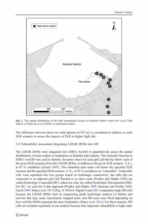
For the conterminous U.S. and parts of Alaska, the current official vertical datum is thegeodetic North American Vertical Datum of 1988 (NAVD88) used for deriving orthometricheights above or below a geoid model. Hawai‘i is an exception to this unified referencedatum in that more traditional methods are used when defining its vertical datum, in whichelevations are referred to Local Tidal Datum (NOAA 2008). This means that orthometricheights in Hawai‘i are considered to be above Local Tidal Datum of MSL. A certain phase ofthe tide defines a modeled elevation called a tidal datum (NOAA 2010), which is transferredinland to local tidal benchmarks using the method of differential leveling (NOAA 2001).The spatial distributions for the tidal benchmarks are in close approximation, with thefurthest tidal benchmark at a distance of only ∼650 m from the Kahului Harbor tide station(Fig. 2). Tidal datums are managed by NOAA National Oceanic Service (NOS) Center forOperational Oceanographic Products and Services (CO-OPS). CO-OPS tidal stations arelocated on U.S. Pacific and Atlantic coasts, the Gulf of Mexico, islands in the Atlantic andPacific Oceans, Alaska and Hawai‘i.
Inundation mapping should be referenced to the tidal datum of Mean High Water(MHW) for the worst-case scenario (NOAA 2001). However, because Hawai‘i expe-riences semidiurnal tides, this study uses Mean Higher High Water (MHHW). MHHWis the average of the higher high water height observations of each tidal day at acontrol tide station, such as the Kahului Harbor tide station, over a 19-year NationalTidal Datum Epoch (http://tidesandcurrents.noaa.gov/mhhw.html). Due to rising sealevel, the National Tidal Datum Epoch was established for monitoring change inglobal sea level (NOAA 2009).
The current tidal epoch at the Kahului Harbor tide station on Maui Island is the tidalepoch of January 1983 to December 2001. The tidal datum of MHHW for this epoch is1.422 m above the Station Datum, and the tidal datum of MSL for this epoch is 1.075 mabove the Station Datum. Tidal datums are referenced to a fixed base established at anelevation below the water known as the Station Datum (http://tidesandcurrents.noaa.gov/).
Climatic Change
The difference between these two tidal datums (0.347 m) is considered in addition to eachSLR scenario to assess the impacts of SLR at higher high tide.
3.4 Vulnerability assessment integrating LiDAR DEMs into GIS
The LiDAR DEMs were integrated into ESRI’s ArcGIS to quantitatively assess the spatialdistributions of areas subject to inundation on Kahului and Lahaina. The reclassify function inESRI’s ArcGIS was used to identify elevation values for each grid cell that lay below each ofthe given SLR scenarios from the LiDAR DEMs, in addition to the given SLR scenario +L.E.Zat 95 % confidence (Gesch 2009). This identified each raster cell below the specified SLRscenario and the specified SLR scenario +L.E.Z at 95 % confidence as “vulnerable”. Vulnerablecells were separated into two groups based on hydrologic connectivity: the cells that areconnected to an adjacent grid cell flooded or in open water (Poulter and Halpin 2008) arecalled Hydrologic Connected (HC); otherwise, they are called Hydrologic Disconnected (HD).For HC, we used the 8-side approach (Poulter and Halpin 2008; Henman and Poulter 2008;Gesch 2009; Marcy et al. 2011) (Fig. 3). NOAA, Digital Coast (2011) separately maps HD cellsbecause the LiDAR DEMs lack an engineering grade hydrologic analysis of ditches andculverts that may cause inaccurately mapped areas, and HD areas may flood depending onhow well the DEMs represent the area’s hydraulics (Marcy et al. 2011). For these reasons, HDcells are included separately in our analysis because they represent vulnerability to high water
Fig. 2 The spatial distribution of the tidal benchmarks located at Kahului Harbor where the Local TidalDatum of Mean Sea Level (MSL) is transferred inland
Climatic Change

tables and poor drainage. Eight Geographic Information System (GIS) vulnerability layers wereproduced using the raster to polygon function in ESRI’s ArcGIS, depending on whether we areconsidering 1) HC or HD areas, 2) best-case (+0.75 m) or worst-case (+1.9 m) SLR scenarios,and 3) with or without the vertical uncertainty L.E.Z at 95 % confidence.
The intersect function in ESRI’s ArcGIS was used to intersect vulnerable layers with GISlayers obtained from the Hawai‘i Statewide GIS Program such as major and minor roads andland parcels. The total land area and length of roads impacted were calculated by taking thesum of the total area and length of roads within each of the vulnerability layers. The land andbuilding value impacted within each parcel was assessed by multiplying the total land andbuilding value within a parcel by the ratio of vulnerable area within the parcel to the totalparcel area (Zhang et al. 2011). The total land and building value impacted within each of thevulnerability layers was then calculated by taking the sum of these values.
4 Results and discussion
4.1 Impacts of original vs. refined DEMs on inundation mapping
Poulter and Halpin (2008) suggested that LiDAR post-processing could influence inunda-tion analysis. This study found that quantifying low-lying lands vulnerable to inundation dueto SLR scenarios is liable to change because of filtering methods that classify the LiDARpoint cloud into ground and non-ground returns. The filtering methods were most influentialat the worst-case SLR scenario of +1.9 m and +1.9 m +L.E.Z at 95 % confidence whencompared to the best-case SLR scenario of +0.75 m and +0.75 m +L.E.Z at 95 % confidencefor hydrologically connected (HC) areas (Table 1). The topographic anomalies caused byinterpolating vegetated areas misclassified as ground returns resulted in less area inundatedalong Kanaha Beach Park in the original USACE DEM at the worst-case SLR scenarioof +1.9 m and +1.9 +L.E.Z at 95 % confidence. Reclassifying the points located withinvegetated areas as non-ground returns removed the topographic anomalies from the refinedUSACE DEM, thus causing more land area to be inundated at the worst-case SLR scenarioof +1.9 m and +1.9 m +L.E.Z at 95 % confidence. Since no more than ground returns wereavailable from the data providers, another round of filtering may have reduced the commis-sion errors of ground returns. Commission errors are when features such as vegetation areclassified as ground-returns when they should not be classified as ground returns. Instead, thesefeatures should be classified as non-ground returns. However, another round of filtering cannotreduce the omission errors because only ground-returns were available from the data serviceprovider. Although the difference in land area inundated between the original and refined
Fig. 3 The 8-side approach used to determine areas with hydrologic connection (HC) to the ocean
Climatic Change

USACEDEM for theworst case SLR scenario of +1.9m and +1.9 m +L.E.Z at 95% confidenceseems small (<5 %), the difference in impacts to land and building value is significant for theSLR scenario of +1.9 m (up to ∼15 %, see Table 2).
4.2 Using tidal benchmarks to correct LiDAR elevations
The RMSE calculated for the USACE LiDAR point data and the refined USACE DEM werethe same; 0.23 m (Table 3). The RMSE of 0.23 m was used in Eq. 2 for the USACE LiDARto calculate a L.E.Z of ±0.45 m at 95 % confidence. The L.E.Z of ±0.318 m at 95 %confidence reported in the NOAA LiDAR metadata was considered. When the L.E.Z at95 % confidence upper bound is added to the specified SLR scenario, additionalelevation would be vulnerable (Figs. 4 and 5) given the vertical uncertainty of theLiDAR data (Gesch 2009).
From the original 10 tidal benchmarks used to define the Local Tidal Datum onMaui Island, one tidal benchmark was removed from analysis due to a lack of LiDARpoints located within a 2 m radius. LiDAR point data within each of the remaining 9tidal benchmarks ranged from 1–12 points (Table 3). Although the tidal benchmarksare located in a flat area, the LiDAR point elevation within a 2 m radius of each tidalbenchmark ranges 0–0.16 m. The mean difference in elevation of the tidal bench-marks and LiDAR points was equivalent to the mean difference of the tidal bench-marks and the refined USACE DEM at 0.09 m. The average difference between theUSACE LiDAR points and the tidal benchmarks is small (0.09 m) and not significantat the 0.05 levels (Table 3), meaning that no corrections had to be made to the refinedUSACE DEM.
Table 1 Difference in land area inundated between the original and refined USACE DEM for Kahului, Maui.MHHW 0Mean Higher High Water (1983–2001 epoch), L.E.Z 95 %00.45 m, HC 0 hydrologically connectedareas, and HD 0 hydrologically disconnected areas
Original Refined Original Refined Original Refined Original Refined
MHHW +0.75 m
MHHW +0.75 m
MHHW +0.75 m + L.E.Z
MHHW +0.75 m+L.E.Z
MHHW +1.9 m
MHHW +1.9 m
MHHW +1.9 m + L.E.Z
MHHW +1.9 m + L.E.Z
Impacts HC HD HC HD HC HD HC HD HC HD HC HD HC HD HC HD
Land (km2) 0.06 0.49 0.06 0.49 0.09 0.83 0.09 0.86 1.95 0.12 2.03 0.1 2.94 0.07 2.98 0.08
Table 2 Difference in impacts to land and building value (over hydrologically connected areas) between theoriginal and refined USACE DEM for Kahului, Maui. MHHW 0 Mean Higher High Water (1983–2001epoch), and L.E.Z 95 %00.45 m
MHHW + 1.9 m MHHW + 1.9 m + L.E.Z
Impacts Original Refined Original Refined
Land (km2) 1.95 2.03 2.94 2.98
Land value ($) 194,268,694 214,183,202 356,048,216 369,017,038
Building value ($) 52,449,815 60,197,247 150,181,331 154,525,815
Climatic Change

In Northwest Maui, the USACE LiDAR within the perimeters of basketball courts,tennis courts, roads and parking lots ranged from 64–288 points, while the NOAALiDAR ranged from 15–72 points (Table 4). The lower point density of the NOAALiDAR in Northwest Maui may confirm an over-classification of the data to removeinfrastructure and vegetation. Another possible reason is that the two datasets origi-nally have different point density. The NOAA average surface elevation was found tobe significantly higher (mean difference of 0.38 m) than the USACE average surfaceelevation at the 0.05 levels (Table 4). This value was applied to correct the NOAADEM.
This method of using the tidal benchmarks near a tide station to assess the verticalaccuracy of the LiDAR proves useful for other low-lying communities considering SLR. Forinstance, a correction may be needed for the LiDAR because orthometric heights of thevertical datum to which the LiDAR is referenced may vary from local MSL; otherwise,unwarranted errors could be introduced into the SLR vulnerability maps (Poulter and Halpin2008; Gesch 2009). This method provides an approach to address the many problemsassociated with lacking an established vertical datum, and may be particularly relevant forother islands.
For the purpose of SLR vulnerability mapping, problems to consider when working withtidal datums include that there are many variations such as MLLW, MSL, MHW, or MHHW.In addition, each variation of a tidal datum may refer to the current epoch of 1983–2001 or asuperseded epoch such as 1960–1978. For the state of Hawai‘i, each tidal datum has uniquevalues to each epoch where the superseded epoch is lower than the current epoch becauseglobal sea level has been slowly rising. As an example, the tidal datum of MSL forthe 1960–1978 epoch on Maui Island is 1.039 m, and the tidal datum of MSL for the1983–2001 epoch on Maui Island is 1.075 m. Another problem in lacking an
Table 3 Elevation differences between tidal benchmarks at the Kahului Harbor tide station, USACE LiDARpoint data and refined USACE DEM. n 0 total number of LiDAR points, Zmin and Z max 0 the minimum andmaximum LiDAR point elevation, Zμ represents the mean elevation of LiDAR points, ZDEM 0 the refinedUSACE DEM elevation, ZBM 0 the tidal benchmark elevation, Δpts 0 the elevation difference between themean elevation of LiDAR points and the tidal benchmark (Zμ - ZBM), and ΔDEM 0 the elevation differencebetween the refined USACE DEM and the tidal benchmark in meters (ZDEM - ZBM). RMSE means root meansquare error
Tidal Benchmark LiDAR points ZDEM ZBM Δpts ΔDEM
n Zmin Zmax Zσ Zμ
161 5680 A 1 2.15 2.15 0.00 2.15 2.11 1.93 0.22 0.18
161 5680 C TIDAL 6 1.65 1.85 0.07 1.77 1.76 1.46 0.31 0.3
161 5680 TIDAL 11 9 2.02 2.11 0.03 2.05 2.06 2.11 −0.06 −0.05161 5680 TIDAL 12 8 1.68 1.81 0.04 1.75 1.76 1.37 0.38 0.39
161 5680 TIDAL 2 12 2.15 2.23 0.03 2.19 2.2 2.50 −0.31 −0.3161 5680 TIDAL 5 12 2.05 2.18 0.04 2.11 2.11 1.86 0.25 0.25
161 5680 TIDAL 6 3 2.58 2.61 0.02 2.59 2.58 2.41 0.18 0.17
161 5680 TIDAL 8 5 2.64 2.71 0.03 2.67 2.67 2.80 −0.13 −0.13161 5680 TIDAL 9 7 2.50 2.66 0.06 2.56 2.54 2.58 −0.02 −0.04Mean 0.09 0.09
RMSE 0.23 0.23
Climatic Change

established vertical datum is that each tidal datum varies from island to island. TheLiDAR is vertically referenced to the Local Tidal Datum, yet there is no foundationto which island, which tidal datum, and which epoch is used. These inconsistenciescould affect vertical accuracy assessment of the LiDAR and when applying differentinundation scenarios, the accuracy of SLR vulnerability maps may be reduced. TheNGS was consulted for this study to verify the lack of a vertical datum for Hawai‘i.This study calls for an established vertical datum among the Hawaiian Islands that
Fig. 4 SLR vulnerability maps of Kahului, Maui, highlighting lands vulnerable under the best-case SLR scenarioof +0.75 m, and the worst-case SLR scenario of +1.9 m. The linear error (L.E.Z) at 95 % confidence upper bound(0.45 m) estimates the vertical uncertainty of the elevation data at each SLR scenario contour. Vulnerable areas areseparated by hydrologic connection (HC) and hydrologic disconnection (HD) from the ocean
Climatic Change

proves important for other islands and low-lying coastal communities considering SLRso that consistent and accurate vulnerability maps can be produced.
Fig. 5 SLR vulnerability maps of Lahaina, Maui, highlighting lands vulnerable under the best-case SLRscenario of +0.75 m, and the worst-case SLR scenario of +1.9 m. The linear error (L.E.Z) at 95 %confidence upper bound (0.318 m) estimates the vertical uncertainty of the elevation data at each SLRscenario contour. Vulnerable areas are separated by hydrologic connection (HC) and hydrologic discon-nection (HD) from the ocean
Table 4 Analysis of ten locations with ≤6 % slope in Northwest Maui between the NOAA and USACELiDAR point data. μ and σ are the mean and standard deviation of n NOAA or USACE LiDAR points, andΔμ 0 the difference between the mean NOAA and USACE LiDAR point elevations (NOAAμ - USACEμ)
Description Feature area (m2) Location(UTM, Zone 4, NAD 83)
Slope% ZNOAA (m) ZUSACE (m) Δμ (m)
μ σ n μ σ n
Basketball court 122 744,014E, 2,324,251N 1-3 13.81 0.04 67 13.58 0.04 288 0.23
Parking lot 28 745,401E, 2,324,650N 1-6 72.16 0.06 15 71.76 0.10 80 0.40
Road 1 64 742,909E, 2,324,005N 4-6 32.13 0.13 34 31.91 0.16 260 0.22
Road 2 44 744,475E, 2,324,740N 3-6 18.00 0.12 40 17.59 0.10 126 0.41
Road 3 38 746,284E, 2,326,341N 3-6 57.06 0.09 27 56.47 0.10 117 0.59
Road 4 26 743,170E, 2,324,064N 3-5 50.97 0.07 19 50.65 0.09 68 0.32
Road 5 58 745,393E, 2,325,407N 6 21.91 0.20 51 21.45 0.20 67 0.46
Tennis court 1 43 743,491E, 2,324,279N 1-3 19.91 0.03 29 19.53 0.06 116 0.38
Tennis court 2 93 742,733E, 2,323,622N 1-3 13.53 0.04 72 13.15 0.03 112 0.38
Tennis court 3 38 745,081E, 2,324,552N 1-5 48.16 0.06 35 47.73 0.05 64 0.43
Mean 0.38
Climatic Change

4.3 Quantitative assessment of vulnerability
Due to lower elevation on the north shore of Maui and larger study area, the inundation of totalland area is greatest in Kahului when compared to Lahaina under each of the SLR scenarios(Tables 5 and 6). The overall impact to land value is greatest in Lahaina when compared toKahului due to higher land value and greater tourist income associated with the high-valuetourist beaches and active tourism industry of Lahaina. Most notable is the land and buildingvalue for Kahului is greater for HD than HC areas under the best-case SLR scenario of +0.75 mand +0.75m +L.E.Z at 95% confidence due to low relief areas just inland from the sea (Table 5).The impact to land value for Lahaina is consistently greater for HC than HD areas under each ofthe SLR scenarios and each of the SLR scenarios +L.E.Z at 95 % confidence (Table 6).
4.4 Vulnerability mapping and adaptation measures
Under the best-case SLR scenario of +0.75 m for HC areas (Fig. 4), the Kahului Harbor andshoreline will be inundated leading to beach erosion and beach loss. Under the best-case SLRscenario of +0.75 m plus L.E. at 95 % confidence for HC areas, more shoreline will beinundated at Kahului Harbor and inundation expands further inland near Kanaha Beach Park.Under the best-case SLR scenario of +0.75 m for HD areas, saltwater intrusion will signifi-cantly impact the freshwater Kanaha Pond Wildlife Sanctuary by threatening endan-gered bird species habitat. Under the best-case SLR scenario of +0.75 m +L.E.Z at95 % confidence for HD areas, Kanaha Pond expands but does not open to the ocean.Expansion is likely driven by rise of the water table, which may be accompanied bysaltwater intrusion through the ground. Research by Rotzoll et al. (2008) demonstratesthat the coastal groundwater table responds to tide forcing and sits near to groundlevel in many locations on the Maui Coast. Rotzoll and El-Kadi (2008) also observedthat wave-setup influences coastal groundwater tables as far inland as 5 km in centralMaui. Vulnerability maps may allow for managers to identify and protect areas alongwith additional wildlife conservation efforts where the Sanctuary is likely to expand.
Under both the worst-case SLR scenario of +1.9 m and the worst-case SLRscenario of +1.9 m +L.E.Z at 95 % confidence for HC areas (Fig. 4), the commercialharbor will be adversely impacted by inundation. The harbor may experience changesin hydraulic characteristics such as swell and tide surge, inundation of facilities, andloss of operating hours. Coastal planners may be able to identify facilities that need tobe relocated by moving further back from the coast in a planned retreat (Nicholls2011).
Table 5 The impacts of sea-level rise on Kahului, Maui, under the best-case SLR scenario of +0.75 m, andthe worst-case SLR scenario of +1.9 m. MHHW 0 Mean Higher High Water (1983–2001 epoch), L.E.Z95 %00.45 m, HC 0 hydrologically connected areas, and HD 0 hydrologically disconnected areas. * Landincludes wetlands
Impacts MHHW + 0.75 m MHHW + 0.75 m + L.E.Z MHHW + 1.9 m MHHW + 1.9 m + L.E.Z
HC HD HC HD HC HD HC HD
Land (km2)* 0.06 0.49 0.09 0.86 2.03 0.1 2.98 0.08
Roads (km) 0.01 0 0.01 0.04 8.86 0.61 15.22 0.08
Land value ($) 3,329,879 14,030,458 6,205,975 32,104,620 214,183,202 13,590,455 369,017,038 5,896,246
Building value ($) 194 k 1,160,944 321 k 5,248,656 60,197,247 7,667,064 154,525,815 1,400,009
Climatic Change

Under both the best-case SLR scenario of +0.75 m and the best-case SLR scenarioof +0.75 m +L.E.Z at 95 % confidence for HC areas (Fig. 5), the Lahaina Harbor andshoreline will be inundated leading to beach erosion and beach loss, which may impactvisitors to the Island seeking prime beaches and recreational activities. Under both the worst-case SLR scenario of +1.9 m and the worst-case SLR scenario of +1.9 m +L.E.Z at 95 %confidence for HC areas, the Hono a Pi‘ilani Highway, coastal roads, residential neighbor-hoods, local businesses and resorts will be inundated and suffer drainage problemsleading to adverse impacts to Lahaina’s tourism industry. Under the worst-case SLRscenario of +1.9 m +L.E.Z at 95 % confidence HD, these areas probably will not beflooded by waves but will materialize as areas lacking drainage where the ocean risesthrough the storm drain system and prevents runoff from draining, which will likelybe accompanied by rise of the water table.
High-resolution SLR vulnerability maps (Figs. 4 and 5) are important to demonstrating low-lying coastal communities’ vulnerability to SLR. Such maps highlight the critical need to takeaction in improving community resiliency to climate change and provide guidance on locationswhere vulnerability is high and underpin decision making for adaptation steps. SLR vulnera-bility mapping can help coastal planners consider the impacts of SLR by highlighting thelowest-lying lands and the critical infrastructure vulnerable to inundation and erosion. Thisallows for the proper adaptation measures to be taken, which may involve relocating coastalcommunities, housing, major and minor roads, local businesses, and ports located within eachof the inundation zones. Relocating beachfront high-rise resorts further from the coast will be adifficult challenge. Decision makers could reduce vulnerability by decreasing development oncoastal areas that are also considered high-risk, as featured on the SLR vulnerability maps.Using science-based setback rules, coastal planners in Maui County determine constructionsetbacks using erosion hazard maps (Genz et al. 2007). Following this example, steps could alsoinclude changing building codes to adopt revised base-flood elevations that incorporate SLR;retro-fitting transportation venues to avoid flooding, especially at traffic volume choke-points.High-resolution SLR vulnerability mapping is important to guiding any coastal community’sadaptive strategies to climate change.
5 Conclusions
Using LiDAR for SLR vulnerability assessments presents many challenges. It is important tounderstand how LiDAR data are collected and post-processed in order to create reliableDEM products for inundation analysis, thus the significance of accurate and informativemetadata. Questioning the quality of the LiDAR data may result in better understanding ofhow the data may influence inundation analysis. This study found that the post-processing
Table 6 The impacts of sea-level rise on Lahaina, Maui, under the best-case SLR scenario of +0.75 m, andthe worst-case SLR scenario of +1.9 m. MHHW 0 Mean Higher High Water (1983–2001 epoch), L.E.Z95 %00.318 m, HC 0 hydrologically connected areas, and HD 0 hydrologically disconnected areas
Impacts MHHW + 0.75 m MHHW + 0.75 m + L.E.Z MHHW + 1.9 m MHHW + 1.9 m + L.E.Z
HC HD HC HD HC HD HC HD
Land (km2) 0.04 0.002 0.05 0.007 0.34 0.03 0.52 0.03
Roads (km) 0.01 0 0.02 0.03 4.36 0.04 6.56 0.01
Land value ($) 50,780,093 2,546,572 77,750,071 5,338,930 323,559,652 6,250,192 489,084,020 7,705,300
Building value ($) 1,297,342 2,878,169 2,258,712 4,710,864 61,082,387 3,480,334 106,621,421 4,993,914
Climatic Change

methods that filter the LiDAR point cloud into classified ground and non-ground returns usedfor DEM generation influence inundation analysis. Examining by visual inspection the qualityof previous filtering results may identify problems where the commission errors of ground-returns identification can be reduced, which may improve SLR vulnerability assessments.
In the great majority of areas around the world lacking an established vertical datum, or withan outdated vertical datum, a relationship between high accuracy LiDAR and tide stationreferences must be established. For Kahului Harbor on Maui Island, adjustments made fromgeoid heights to the Local Tidal Datum of MSL were successful. For future SLR vulnerabilitymapping, an established vertical datum would allow for more rigorous vertical accuracyassessments and merging of multiple LiDAR datasets located anywhere in the state.
If no adaptive strategies are taken, inundation due to SLR will lead to adverse socioeco-nomic impacts on Kahului and Lahaina. Under the best-case SLR scenario of +0.75 m forHC and HD areas combined, an impact to land and building value of $18.7 million ispossible due to the inundation of 0.55 km2 of area for Kahului, and an impact of $57.5million is possible due to the inundation of 0.04 km2 of area for Lahaina. As would beexpected, adverse socioeconomic impacts to Kahului’s commercial district and Lahaina’stourism industry are most profound for the worst-case SLR scenario of +1.9 m. Under thisworst-case SLR scenario for HC and HD areas combined, an impact to land and buildingvalue of $296 million is possible due to the inundation of 2.13 km2 of area for Kahului(which will also lead to wetland loss), and an impact of $394 million is possible due to theinundation of 0.37 km2 of area for Lahaina. Our study demonstrates that there is acompelling need to improve community resiliency to SLR. Coastal planners in Hawai‘icould require SLR vulnerability assessments as a first step toward building resiliency.
Improvements for future SLR vulnerability assessments may include up-to-date socio-economic GIS data and mapping of the water table. For instance, GIS data of the spatialdistributions of the Gross Domestic Product (GDP) by individual county, building footprints,population in each household, power stations, sewage, commuter density, traffic choke-points, hospitals, evacuation routes, cultural sites, endangered species and imperiled eco-systems will serve useful for future SLR vulnerability assessments. Mapping of the watertable and improved understanding of tidal and seasonal processes associated with verticalwater table movement will improve vulnerability assessment of both HC and HD areas forthe purpose of flood drainage and runoff engineering. Overall, SLR vulnerability mappingraises awareness of the potential impacts of SLR to the community, economy, and habitats ofislands, and provides a valuable tool for coastal communities and policy makers consideringadaptation strategies.
Acknowledgments We appreciate comments by three anonymous reviewers. Data were provided by theNOAA CSC, NGS, Hawai‘i Statewide GIS Program, and DigitalGlobe. This study was funded by a grantfrom the U.S. Department of Interior Pacific Islands Climate Change Cooperative.
References
ASPRS (2004) ASPRS guidelines vertical accuracy reporting for LiDAR data, vol.1.0. http://www.asprs.org/a/society/committees/standards/standards_comm.html. Accessed 22 August 2011
CCSP (2009) Synthesis and assessment product 4.1: coastal sensitivity to sea-level rise: a focus on the Mid-Atlantic region. U.S. Climate Change Program, Washington, DC
Chen Q (2007) Airborne LiDAR data processing and information extraction. Photogramm Eng Rem Sens73:109–112
Climatic Change

Chen Q, Gong P, Baldocchi DD, Xie G (2007) Filtering airborne laser scanning data with morphologicalmethods. Photogramm Eng Rem Sens 73:171–181
FGDC (1998) Geospatial positioning accuracy standards, Part 3. National Standard for Spatial Data Accuracy.FGDC-STD-007.3-1998. http://www.fgdc.gov/standards/projects/FGDC-standards-projects/accuracy/part3/index_html. Accessed 22 August 2011
Fletcher CH (2009) Sea level by the end of the 21st century: a review. Shore & Beach 77:4–12Fletcher C, Boyd R, Grober-Dunsmore R, Neal WJ, Tice V (2010) Living on the shores of Hawai‘i. University
of Hawai‘i Press, HonoluluGenz AS, Fletcher CH, Dunn RA, Frazer LN, Rooney JJ (2007) The predictive accuracy of shoreline change rate
methods and alongshore beach variation on Maui, Hawaii. J Coast Res 23:87–105. doi:10.2112/05-0521.1Gesch DB (2009) Analysis of LiDAR elevation data for improved identification and delineation of lands
vulnerable to sea-level rise. J Coast Res 53:49–58. doi:10.2112/S153-006.1GOF (2011) The Global Oceans Forum report of activities 2010. www.globaloceans.org. Accessed 22 august
2011Henman J, Poulter B (2008) Inundation of freshwater peatlands by sea level rise: Uncertainty and potential
carbon cycle feedbacks. J Geophys Res 113:G01011. doi:10.1029/2006JG000395IPCC (2007) Climate change 2007, the physical science basis. Cambridge University Press, CambridgeLiu XY (2011) Accuracy assessment of LiDAR elevation data using survey marks. Surv Rev 43:80–93.
doi:10.1179/003962611X12894696204704Marcy D, Brooks W, Draganov K, Hadley B, Haynes C, Herold N, McCombs J, Pendleton M, Ryan S,
Schmid K, Sutherland M, Waters K (2011) New mapping tool and techniques for visualizing sea level riseand coastal flooding impacts. In: Wallendorf LA, Jones C, Ewing L, Battalio B (eds) Proceedings of the2011 Solutions to Coastal Disasters Conference, Anchorage, Alaska, June 26 to June 29, 2011., pp 474–90, Reston, VA: American Society of Civil Engineers. http://csc.noaa.gov/digitalcoast/tools/slrviewer/support.html#cite1. Accessed 17, March 2012
McLeod E, Poulter B, Hinkel J, Reyes E, Salm R (2010) Sea level-rise impact models and environmentalconservation: a review of models and their applications. Ocean Coast Manage 53:507–517. doi:10.1016/j.ocecoaman.2010.06.009
Maune DF (2007) DEM User Requirements. In: Maune DF (ed) Digital elevation model technologies andapplications: the DEM users manual, 2nd edn. American Society for Photogrammatry and RemoteSensing, Bethesda, pp 449–473
Nicholls RJ (2011) Planning for the impacts of sea level rise. Oceanography 24:144–157. doi:10.5670/oceanog.2011.34
NOAA (2001) Tidal datums and their applications. NOAA special publication NOS CO-OPS 1. NOAANational Ocean Service, Silver Spring
NOAA (2008) Topographic and bathymetric data considerations: datums, datum conversion techniques, anddata integration. Technical Report NOAA/CSC/20718-PUB. National Oceanic and Atmospheric Admin-istration, Charleston, SC
NOAA (2009) Sea level variations of the United States 1854–2006. Technical Report NOS CO- OPS 053.NOAA National Ocean Service, Silver Spring
NOAA (2010) Technical considerations for use of geospatial data in sea level change mapping and assess-ment. NOAA NOS Technical Report. NOAA National Ocean Service, Silver Spring
NOAA (2011) Digital Coast, NOAA Coastal Services Center. http://csc.noaa.gov/digitalcoast/tools/slrviewer/support.html#cite1. Accessed 17, March 2012
Poulter B, Halpin PN (2008) Raster modeling of coastal flooding from sea-level rise. Int J Geogr Inf Sci22:167–182. doi:10.1080/13658810701371858
Rotzoll K, El-Kadi AL (2008) Estimating hydraulic properties of coastal aquifers using wave setup. J Hydrol353:201–213. doi:10.1016/j.jhydrol.2008.02.005
Rotzoll K, El-Kadi AL, Gingerich SB (2008) Analysis of an unconfined aquifer subject to asynchronous dual-tide propagation. Ground Water 46:239–250. doi:10.1111/j.1745-6584.2007.00412.x
US Census Bureau (2011) The 2011 statistical abstract of the United States. US Census Bureau. Washington,DC. http://www.census.gov/compendia/statab/. Accessed 22 August 2011
Vermeer M, Rahmstorf S (2009) Global sea level linked to global temperature. Proc Natl Acad Sci106:21527–21532. doi:10.1073/pnas/.0907769106
Wu SY, Yarnal B, Fisher A (2002) Vulnerability of coastal communities to sea-level rise: a case study of CapeMay County, New Jersey, USA. Clim Res 22:255–270
Zhang K (2011) Analysis of non-linear inundation from sea-level rise using LiDAR data: a case study forSouth Florida. Clim Change 106:537–565. doi:10.1007/s10584-010-9987-2
Zhang K, Dittmar J, Ross M, Bergh C (2011) Assessment of sea level rise impacts on human population andreal property in the Florida Keys. Clim Change 107:129–146. doi:10.1007/s10584-011-0080-2
Climatic Change