• • • • • • • • • • • • • • • • • • • • • • • • • • • • • • • • •

RECORD 1993/37

Assembling the Ebagoola 1 :250,000 Integrated Dataset in ER Mapper

Prame N. Chopra Information Systems Branch

II 11111111 ~ • *R9303701*

DEPARTMENT OF PRIMARY INDUSTRIES AND ENERGY

Minister for Resources: The Hon. Michael Lee Secretary: Greg Taylor

AUSTRALIAN GEOLOGICAL SURVEY ORGANISATION

Executive Director: Roye Rutland

© Commonwealth of Australia

ISSN: 1039-0073

ISBN: 0 642 19320 7

This work is copyright. Apart from any fair dealings for the purposes of study, research, criticism or review, as permitted under the Copyright Act, no part may be reproduced by any process without written permission. Copyright is the responsibility of the Executive Director, Australian Geological Survey Organisation. Inquiries should be directed to the Principal Information Officer, Australian Geological Survey Organisation, GPO Box 378, Canberra City, ACT, 2601.

• • • • • • • • • • • • • • • • • • • • • • • • • • • • • • • • • •

• • • • • • • • • • • • • • • • • • • • • • • • • • • • • • • • • •

Table of Contents

Introduction

Importing dxf Files from Intergraph

Importing FS Images

Building a Map from a dxfFile

Creating an Arc/Info Coverage from a dxf File

Magnetics.ers and magnetics

Radiometrics.ers and radiometries

Annotation overlays

J2S Processing History Ebagoola Magnetics and Radiometries

Ebagoola.image - Processing History

Magnetics.image - Processing History

Acknowledgements

References

Figure 1 The main data flows involved in assembling the Ebagoola NGMA integrated dataset in ER Mapper

Table 1 An example of output from the Arc/Info dxfinfo command

3

PAGE

4

5

8

8

9

11

12

13

14

14

16

17

17

5

9

Abstract

Available digital geoscience data for the Ebagoola 1 :250,000 sheet, Cape York Peninsula were assembled in fonnats compatible with the ER Mapper image processing software. These data included raster datasets such as LANDSAT TM, processed airborne radiometric and magnetic data and grids of stream sediment geochemistry data. Vector datasets included drainage, the results of geological and regolith field mapping and known mineral occurrence point data.

The data processing and data conversion steps that were followed in importing each dataset into ER Mapper are the subject of this Record.

Introduction

The different digital datasets that eventually made up the Ebagoola 1 :250,000 integrated dataset had been compiled or copied onto a range of spatial information technology (IT) systems within AGSO. Raster data resided on the 12S image processing system and the ARGUS airborne processing system. Vector data were stored in the ArclInfo geographic information system and the Intergraph digital cartography system. Point data were held in the Oracle relational database management system. Details of these IT systems and of the links between them are presented by Moore et al (1992). Procedures for the import and export of data between the ER Mapper image processing system and AGSO's other main spatial IT systems are described in detail by Chopra (1993).

The procedures that are described here should have general applicability for other projects. Note however that there is often more than one way to achieve the same result. The procedures described here should therefore not be seen as the only way to approach a given problem.

A data flow diagram showing the sources of the data that were assembled for the Ebagoola 1 :250,000 NGMA integrated dataset and the main import/export procedures that were used is shown in Figure 1.

A note on conventions used here: I have used bold type for user inputs and nonnal type for system responses and my explanatory comments. The latter comments are often enclosed within parentheses () to separate them from system output.

4

• • • • • • • • • • • • • • • • • • • • • • • • • • • • • • • • • •

}Em. M®JWJW®IT' *I~'-I loverlays/Addldxf I

arcdxf

AIT'~!nIlllli@

I dxfarc I

I dlsk'read'geomag I

IIII§

*Utll1tles/Import Rasterl lIS S600

Figure 1 The main data flows involved in assembling the Ebagoola NOMA integrated dataset in ER Mapper.

Importing dxf Files from Intergraph

The file ebag_geol_250000 and ebag~eol_250000.erv are derived ultimately from a dxf file called d5412geo.dxf provided by CSU. The file contains the vectors for the Ebagoola 1:250000 sheet geology as at 29 July 1992.

The dxf file was in units of km so I imported it into ArclInfo and transformed it into metres (see below). I then exported the cover from arc as a dxf file (using arcdxf) and imported it into ER Mapper using:

importdxf -D AGD66 -P TMAMG54 -g -v ebagoola_geol_250000_m.dxf ebag_geol_ 250000.erv

The importdxf command is in the /usr/share/enn/ermapper/bin/sun4 directory. To use it and the other ER Mapper executable binaries, add this directory to the UNIX path in your environment. Alternatively, you can run the command from within its directory and specify the input and output dataset's path and name in full. If you take this approach, make sure that the output path you are specifying allows you write access. This latter solution is obviously pretty clumsy, especially when the UNIX paths are long. The best way to modify the UNIX path permanently is to edit the .cshrc file in your home directory (normally on /mnt). Add the line:

source /mnt/protos/cshrc-ermapper

5

to the .cshrc file using an editor like vi or textedit

Note: The geology cover that was created from d5412geo.dxf by using dxfarc is in UTM Zone 54 but the units are kilometres not the usual metres. Apparently, CSU always work with data in kilometres in their Intergraph environment (H. Apps, pers. comm. 1992) so this is likely to be a recurring problem. The data must be transfonned to metres before they can be used in Arc/Info and in J2S and ER Mapper since for all these systems we use metres as the units of distance. The transformation can either be done in the Intergraph system before CSU write the dxf file, or it can be done in Arc/Info after the data in the dxf file have been made into a coverage.

To transform the Arc/Info cover to metres the following steps should be followed:

Arc: create geol_ 250000_ m geol_ 250000 (create a new cover which will be in metres)

Creating coverage geol_250000_m Arc: info INFO EXCHANGE CALL 04/08/1992 14:25:42 INFO 9.42 11/11/86 52.74.63* COPYRIGHT 1986 HENCO SOFTWARE, INC. PROPRIETARY TO HENCO SOFTWARE, INC. US GOVT AGENCIES SEE USAGE RESTRICTIONS IN HELP FILES (HELP RESTRICTIONS) ENTER USER NAME>ARC

ENTER COMNlAND >SEL GEOL 250000 M.TIC 4 RECORD(S) SELECTED

ENTERCO~>L~T

$RECNO IDTIC XTIC 1 1 827.48740 2 2 661.27785 3 3 661.27785 4 4 827.48740

- -

YTIC 8,338.37500 8,338.37500 8,451.75525 8,451.75525

(open the tic file for the new cover)

(the tic points in the new cover)

ENTER COMMAND >UPDATE XTIC,YTIC BY IDTIC PROMPI' IDTIe?>1

1 XTIC = YTIC =

XTIC>827487.4 YTIC>8338375.0 IDTIC?>2

2 XTIC = YTIC =

XTIC>661277.85 YTIC>8338375.0

827.48740 8,338.37500

661.27785 8,338.37500

6

(multiply the tic values by 10(0)

(multiply the tic values bY 1(00)

• • • • • • • • • • • • • • • • • • • • • • • • • • • • • • • • • •

• • • • • • • • • • • • • • • • • • • • • • • • • • • • • • • • • •

IDTIC?>3 3

XTIC = YTIC =

XTIC>661277.85 YTIC>8451755.25 IDTIC?>4

4 XTIC = YTIC =

XTIC>827487.4 YTIC>8451755.25 IDTIC?>

661.27785 8,451.75525

827.48740 8,451.75525

ENTERCO~>LffiT

$RECNO IDTIC XTIC 1 1 827,487.40000 2 2 661,277.85000 3 3 661,277.85000 4 4 827,487.40000

(multiply me tic values by 1000)

(multiply me tic values by 1000)

(The I RETURNI key was pressed on an empty line)

YTIC 8,338,375.00000 8,338,375.00000 8,451,755.25000 8,451,755.25000

(exit INFO and retum to Arc)

The 4 tic points for the new cover have now been multiplied by 1000 and the changes have been saved. The data in the original kilometre cover must now be transformed into the new and still empty, metre cover. To do this we use the transform command in Are, as shown in the following example:

Arc: transform geol_250000 geol_250000_m Transforming coordinates for coverage geoC250000

Scale (X,Y) = (1000.000,1000.000) Translation = (0.000,0.000) Rotation (degrees) = (0.000) RMS Error (input, output) (0.000,0.000)

tic id input x input y output x output y x error y error

------ ---------------- ---------------- ---------- ----------1 827.487 8338.375

827487.400 8338375.000 0.000 0.000 2 661.278 8338.375

661277.850 8338375.000 0.000 0.000 3 661.278 8451. 755

661277.850 8451755.250 0.000 0.000 4 827.487 8451. 755

827487.400 8451755.250 0.000 0.000 Arc:

The new coverage geol_250000_m now has units of metres. Note that the input and output values for x and y differ by a factor of one thousand and that the errors in x and yare zero. If these conditions are not met then something has gone awry. Check in this case that all four of the tic points have been correctly multiplied by 1000.

7

Importing PS Images

The files comp and comp.ers are the Ebagoola 1 :250,000 radiometrics expressed as byte data (i.e. the image is only 8-bit [=256 colours only D. These ER Mapper files were built from an PS image file using the ER Mapper command:

imports600 -v -D AGD66 -P TMAMG54 / dimlu/nq2iprameci ebagoolal original_datal comp.image / dimluinq2iprameci ebagoolalfinal datalcomp.ers

the -v switch means a verbose description of the progress of the import is given the -D switch specifies the geodetic datum to be used for the map projection. Here

we choose AGD66 (the Australian Geodetic Datum, 1966 which is described in the publication: The Australian Geodetic Datum Technical Manual, National Mapping Council of Australia, Special Publication 10, pp 65 plus annexes).

the -P switch specifies the map projection that the image is to be projected into. Here we choose TMAMG54 which stands for Transverse Mercator Australian Map Grid Zone 54.

the file comp.image is the input data file in the original PS flab format the file comp.ers is the name of the ASCII output header file for ER Mapper. Note: A second binary file containing the actual image data is also written. This second fIle has the same name but no .ers extension (i.e. in this case the binary image file is just called comp and it is written into the same directory as the .ers file which in this case is /dlmlu/nq2/pramec/ebagoola/fmal_data/ ).

Building a Map from a dxf File

To build a map from a dxf fIle using Arcplot do the following:

Areplot: map ebagoola_250000 Areplot: map extent dxf I dimluinq2iprameci ebagooIa/ebagoola _ original_datal dS412geo.dxf Areplot: dxf 1d/m1u/nq2/prameciebagoolalebagoola _ original_ dataid5412geo.dxf Reading header ...

Reading line types ... Reading layers .. . Reading styles .. . Reading block definitions ... arcplot:

Note: This procedure produces a displayable map but it does not produce a coverage. Thus, no feature attribute tables are created and it is not possible to perform queries or analyses on the data. If you want to be able to do this, and for most applications in ArclInfo, you will, then you need to follow the steps below.

8

• • • • • • • • • • • • • • • • • • • • • • • • • • • • • • • • • •

• • • • • • • • • • • • • • • • • • • • • • • • • • • • • • • • • •

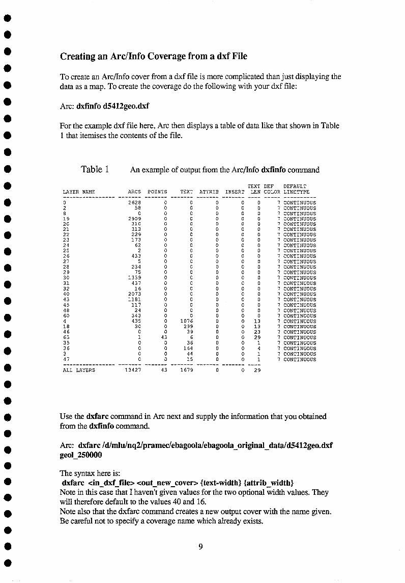
Creating an Arc/Info Coverage from a dxf File

To create an Arc/Info cover from a dxf file is more complicated than just displaying the data as a map. To create the coverage do the following with your dxf file:

Arc: dxfinfo d5412geo.dxf

For the example dxf fIle here, Arc then displays a table of data like that shown in Table 1 that itemises the contents of the file.

Table 1 An example of output from the Arc/lnfo dxfinfo command

TEXT DEF DEFAULT LAYER NAME ARCS POINTS TEXT ATTRIB INSERT LEN COLOR LINE TYPE ---------------- ------- ------- ------- ------- ------- ---- ----- ----------0 2628 0 0 0 0 0 7 CONTINUOUS 2 58 0 0 0 0 0 7 CONTINUOUS 8 0 0 0 0 0 0 7 CONTINUOUS 19 2909 0 0 0 0 0 7 CONTINUOUS 20 310 0 0 0 0 0 7 CONTINUOUS 21 313 0 0 0 0 0 7 CONTINUOUS 22 229 0 0 0 0 0 7 CONTINUOUS 23 173 0 0 0 0 0 7 CONTINUOUS 24 62 0 0 0 0 0 7 CONTINUOUS 25 2 0 0 0 0 0 7 CONTINUOUS 26 433 0 0 0 0 0 7 CONTINUOUS 27 5 0 0 0 0 0 7 CONTINUOUS 28 234 0 0 0 0 0 7 CONTINUOUS 29 75 0 0 0 0 0 7 CONTINUOUS 30 1339 0 0 0 0 0 7 CONTINUOUS 31 437 0 0 0 0 0 7 CONTINUOUS 32 16 0 a a a a 7 CONTINUOUS 40 2073 0 0 a 0 0 7 CONTINUOUS 43 1181 0 a 0 0 0 7 CONTINUOUS 45 117 a 0 0 a 0 7 CONTINUOUS 48 24 0 a 0 0 0 7 CONTINUOUS 60 343 a 0 0 0 0 7 CONTINUOUS 4 435 0 1076 0 0 13 7 CONTINUOUS 18 30 0 299 0 0 13 7 CONTINUOUS 46 0 0 39 0 0 23 7 CONTINUOUS 63 1 43 6 0 0 29 7 CONTINUOUS 35 0 0 36 0 0 1 7 CONTINUOUS 36 0 0 164 0 0 4 7 CONTINUOUS 3 0 0 44 0 0 1 7 CONTINUOUS 47 0 0 15 0 a 1 7 CONTINUOUS ---------------- ------- ------- ------- ------- ------- ----ALL LAYERS 13427 43 1679 0 a 29

Use the dxfarc command in Arc next and supply the information that you obtained from the dxfinfo command.

Arc: dxfarc /dlmlu/nq2/pramec/ebagoolaiebagoola _ original_ dataid5412geo.dxf geol_ 250000

The syntax here is: dxfarc <in _ dxf _file> <out_new _cover> {text-width} {attrib _width}

Note in this case that I haven't given values for the two optional width values. They will therefore default to the values 40 and 16. Note also that the dxfarc command creates a new output cover with the name given. Be careful not to specify a coverage name which already exists.

9

Note: dxfarc can handle a maximum of 999 layers. Layer names can be longer than 16 characters but they must be unique within the first 16. Arcs with more than 500 points will be automatically split into two or more arcs by the dxfarc command. Each arc will have the same User-ID. The dxf entity types Circle and Arc are defined in the dxf me as curves and not all the vertices are stored (i.e. only the feature definition is stored). Hence dxfarc has to calculate appropriate vertices for each entity. To do this, it assigns one vertex for each angular degree traversed by the entity. Hence for a circle, 361 vertices are constructed. Note however that circles defined within blocks in the dxf file will only have 73 vertices (one vertex for every 5 degrees and one vertex to close the circle) which may be too coarse an approximation for some applications. More information on the use of the dxfarc command can be found in the Arc manual and by typing help dxfarc at the Arc: prompt.

the dxfarc command produces the following output for the example dxf file used here:

Enter layer names and options (type END or $REST when done) =======================--====================== Enter the 1st layer and options: 0 all Enter the 2nd layer and options: 2 all Enter the 3rd layer and options : 8 all Enter the 4th layer and options: 19 all Enter the 5th layer and options: 20 all Enter the 6th layer and options: 21 all Enter the 7th layer and options: 22 all Enter the 8th layer and options: 23 all Enter the 9th layer and options : 24 all Enter the 10th layer and options: 25 all Enter the 11th layer and options: 26 all Enter the 12th layer and options: 27 all Enter the 13th layer and options: 28 all Enter the 14th layer and options : 29 all Enter the 15th layer and options: 30 all Enter the 16th layer and options: 31 all Enter the 17th layer and options: 32 all Enter the 18th layer and options : 40 all Enter the 19th layer and options : 43 all Enter the 20th layer and options: 45 all Enter the 21 st layer and options: 48 all Enter the 22nd layer and options: 60 all Enter the 23rd layer and options: 4 all Enter the 24th layer and options : 18 all Enter the 25th layer and options : 46 all Enter the 26th layer and options: 63 all Enter the 27th layer and options: 35 all Enter the 28th layer and options : 36 all Enter the 29th layer and options: 3 all

10

• • • • • • • • • • • • • • • • • • • • • • • • • • • • • • • • • •

• • • • • • • • • • • • • • • • • • • • • • • • • • • • • • • • • •

Enter the 30th layer and options : 47 all Enter the 31st layer and options: END Do you wish to use the above layers and options (YIN)? y

Processing /D/MLU/NQ2/PRAMEC/EBAGOOLA/EBAGOOLA_ ORIGINAL_DAT AJD5412GE O.DXF ...

NOTE: the layer names (here numbers between 0 and 60) came from the dxflnfo command's output (see above). These layer names must only be entered once. The all entry for each layer is actually redundant because it is the default. Instead of using all the user can specify in detail the attributes of the layer. Details such as colour, thickness, line type, and elevation for lines and colour, thickness, type, angle, size and elevation for points can be entered on the line following the layer name. The attribute values must be integers (see Table 1 for examples). The dxfarc command creates INFO files to describe the attributes of points and arcs in the cover generated from the dxf file. These INFO files are called <oucnew_cover>XCODE and <oucnew_cover>.ACODE respectively.

Magnetics.ers and magnetics

These files are the ER Mapper ASCII header and the binary file for an IEEE byte*4 raster of the ebagoola magnetics. The file was produced by: 1) warping an PS file called magnetics.image (also known as p568m.image which was made from the p568m.GRD file from airborne group's ARGUS system) using the PS command: be < iis _warp _mag.com.

The control file iis_ warp_mag.com contained the following lines:

cpu'cpwarp magnetics.image magnetics_ warp.image map_projection

27,15,927,15,1827,15,27,615,927 ,615,1827 ,615,27,1215,927 ,1215,1827,1215 8451755.27,662003.2,8451113.5,743035.66,8450214.29,824105.16,8396439.64,661 646.65,8395776.89,742500.47,8394848.3,823390.91,8341121.82,661277.85,834043 8.3,741946.9,8339480.61,822652.12 nearescneighbor 50 yes yes yes 2

11

The warped FS image had a user coordinate system CUCS) with the following parameters:

Ax = 0.050, Ay = -0.050, Bx = 658.863 and By = 8453.183

These parameters can be read in I2S by using the s'dir -f filename command in the I2S display executive (de).

The FS file was then imported into ER Mapper with the ER Mapper imports600 command (see the details above for how to do this and the discussion by Chopra, 1993). The .ers file that was created by imports600 was then edited to include the lines:

CellInfo Begin Xdimension = 50 Y dimension = 50

CellInfo End

RegistrationCoord Begin Eastings = 658863 Northings = 8453183

RegistrationCoord End

The parameters used in these entries in the .ers file were obtained from the 12S DCS (note the multiplication by 1000 in this case however to convert from km to metres).

Radiometrics.ers and radiometries

The files radiometries and radiometrics.ers were derived in a similar fashion to the magnetics image. Three FS images produced by Peter Milligan in AGSO's Airborne Geophysics Group were merged into a single FS image using cpu'merge in de then the new combined file (radiometrics.image) was warped with cpu'cpwarp in be (using the command be < iis_warp_rad.com) with the control file iis_warp_rad.com which contained:

cpu'cpwarp /dlmlu/nq2/pramec/ebagoola/ebagoola_original_data/radiometrics.image /dlmlu/nq2/pramec/ebagoola/ebagoola_original_data/radiometrics_ warp.image map_projection

1,1,927,1,1853,1,1,627,927,627,1853,627, 1,1253,927,1253,1853,1253 8454167,659678,8453511, 7 43058,8452584,826478,8396455,659311,8395777,74250 0,8394818,825728,8338740,658932,8338040,7 41922,83 37050,824951 nearescneighbor 50 yes

12

• • • • • • • • • • • • • • • • • • • • • • • • • • • • • • • • • •

• • • • • • • • • • • • • • • • • • • • • • • • • • • • • • • • • •

yes yes 2

The resulting warped PS file radiometrics_ warp.image was then read into ER Mapper using:

imports600 -v -D AGD66 -P SUTM54 radiometries_warp.image • .Iebagoola _ fmal_ datalradiometrics.ers

and then, as before, the .ers file was edited to include the lines:

CellInfo Begin Xdimension = 50 Y dimension = 50

Celllnfo End

RegistrationCoord Begin Eastings = 658856 Northings = 8454283

RegistrationCoord End

Annotation overlays

Twenty four ER Mapper annotation overlays were derived from equivalent Arc/Info coverages of geology built by John Wilford from the digiti sing and drafting work of CSU.

There were 24 ArclInfo coverages named geo 1- ge026 (the names ge022 and geo 11 were missing and the name geoll was included). I used the same names for the annotation overlays as had been used for the Arc/Info covers for consistency, even though these names are completely uninformative as to the nature of the data.

Each cover was exported from ArclInfo as a dxf file using:

Arc: arcdxf <out_dxf_tilename> {in-line_cover} {in_point_cover} {in_annotation _cover}

For example: Arc: arcdxf geo14.dxf geo14

This produced a dxf IIle that could then be read into ER Mapper as a vector file using for example:

[19] pchopra /dlmlu/nq2/pramec/ebagoola/ebagoola_finaLdata % importdxf -D AGD66 -p TMAMG54 -g -v geo14.dxf geo14.ers

13

The command line procedure used here to import the dxf files from Arc/Info was much better than the alternative of using the ER Mapper menus and dialog boxes. To have used the latter would have been much more tedious than just changing the numeric part of each filename in the command by using the command editing features of the C shell. For example, the following C shell command:

[20] pchopra /dlmlu/nq2/pramec/ebagoola/ebagoola_fmal_data % !19:gs/14/15/

would convert the importdxf command above to:

[21] pchopra /dlmlu/nq2/pramec/ebagoola/ebagoola_final_data % importdxf -D AGD66 -p TMAMG54 -g -v geo15.dxf geo15.erv

which would perform the import for the next dxf file of Arc/Info data.

The importdxf commands create an Ascn header file (e.g. geoI5.erv) and an associated ASCn data file which contains the actual vector data. The * .erv file contains all the necessary georeferencing information so there is no need to do an edit on this file the way that there is with *.ers files (e.g. when importing images using the imports600 command, see page 8 and page 13).

I2S Processing History Ebagoola Magnetics and Radiometries

Ebagoola.image • Processing History

The * .GRD files were created on the AGSO Data General MV20000 computer and were then uploaded to the Sun computers running the J2S software using the TCPIIP file transfer protocol (ftp).

(Note: P568 stands for project 568 of the Airborne Geophysics Group - the Ebagoola 1 :250,000 sheet)

Once the data were on the 12S software's platform, they were imported into PS flab format and then converted into IEEE 4 byte integers to save disk space. The PS commands used are listed in the following PS log file records as follows:

16:56:25.0 ------------ Log File Opened (8-Aug-1991) 16:56:25.0 * disk'read'geomag P568M.GRD ebagoola_mag.int 19:24:38.0 * disk'read'geomag P568TC.GRD ebagoola_te.int 21:51:12.0 * disk'read'geomag P568K.GRD ebagoola_k.int 00:11:04.0 * disk'read'geomag P568U.GRD ebagoola_u.int 02:37: 16.0 * disk'read'geomag P568TH.GRD ebagoola_th.int 05:05:52.0 ------------ Log File Closed (9-Aug-1991)

12:24:01.0 ------------ Log File Opened (9-Aug-1991) 12 :24:0 1.0 * system'setdefault /hydro3/pramec/ capeyorklorigioal_ data/ebag

* oola

14

• • • • • • • • • • • • • • • • • • • • • • • • • • • • • • • • • •

• • • • • • • • • • • • • • • • • • • • • • • • • • • • • • • • • •

Convert files to BYTE format to save space

12:24:40.0 * cpulscale -out_dtype=BYTE ebagoola_mag.int ebagoola_mag 12:26:34.0 * cpu'scale -out_dtype=BYTE ebagoola_k.int ebagoola_k 12:28:37.0 * cpu'scale -out_dtype=BYTE ebagoola_u.int ebagoola_u 12:30:28.0 * cpu'scale -out_dtype=BYTE ebagoola_th.int ebagoola_th

Merge the 5 files into 1 prior to warping. Note however that the magnetics image is bigger than the others in the X direction. Magnetics is 1853 x 1229 while the radiometric images are 1829 x 1229 The origin of the radiometric images is at the same latitude as the magnetics data, but it is 12 pixels to the east of the magnetics one. Hence, the eastern extent of the radiometric data is also 12 pixels west of the magnetics eastern boundary. (i.e. the magnetics data extend a further 12 pixels on either side of the radiometries data)

13:42:18.0 * cpu1merge -placement=(11112121213 1214 1215) -si * ze=(18531229 5) ebagoola_mag, ebagoola_tc, ebagoola_k * ,ebagoola_th,ebagoola_u ebagoola

Create a control points fIle for the warp by using the 4 corner points of the (larger) magnetics dataset (the radiometric data all fall within these boundaries).

NOTE: this had to be done from the garnet Sun 4/280 because it only worked properly in S600 version 3 (version 4.0 was running on topaz Sun 4/280 at the time).

13:55:53.0 * cpu'gcp'byhand -cnpt_file=ebagoola -create=y -file_type=2-m * apSystem=4 -maxpoints=200

14:02:05.0 * cpu'aux'read -type=cnpt ebagoola.cnpt

Do the warp using the default pixel size of 80 metre because the grid spacing of the data is 8.333333*10-4 decimal degrees which, at this latitude corresponds to approx 83 metre. The warp was also done with a bilinear interpolation. Use the control point file set up previously (i.e. ebagoola.cnpt). The latitude of the origin of the projection used was -0 The false easting given was 500 000 The false northing was 10 000 000 The ellipsoid was 14

14:13:05.0 * cpu'cpwarp -projection=MAP _PROJECTION -cpfiJe _ name=ebagoola.cnpt -order Jnteractive=yes ebagoola ebagoola_ warp

Once the warp has completed (and this may take up to several hours of elapsed time) exit the J2S de by typing quit and return to the UNIX prompt. The old pre-warped version of the image is generally no longer needed, so it can be deleted in UNIX by typing: rm ebagoola.image

15

The new warped version of the dataset can now be renamed by using the UNIX mv command. mv ebagoola _ warp.image ebagoola.image

The warped image ebagoola.image contains all the magnetics and radiometrics data for the Ebagoola airborne survey and all 5 datasets are co-registered. Note however, that these datasets are all in byte format (i.e. 8-bit = 256 colour).

Magnetics.image - Processing History

(originally called p568m.image - an PS reals image from Peter Milligan in the Airborne Geophysics Group)

p568k_f.image p568th_f.image p568u_f.image

floating point K radiometrics for Ebagoola rt 1t Th 1t n 11

" " U " " "

The processing steps taken are again recorded in the following log file records:

16:56:25.0 ------------ Log File Opened (8-Aug-1991) 21:51:12.0 * disk'read'geomag PS68K.GRD radiometrics_k.int 00:11:04.0 * disk'read'geomag PS68U.GRD radiometries_u.int 02:37: 16.0 * disk'read'geomag PS68TH.GRD radiometries_th.int 05:05:52.0 ------------ Log File Closed (9-Aug-1991)

13:42:18.0 * epu'merge -plaeement=(111112113) -si * ze=(1829 1229 5) radiometries _ k * , radiometries _ th, radiometries _ u radiometries

Do the warp using the default pixel size of 80 metre because the grid spacing of the data is 8.333333*10**-4 decimal degrees which, at this latitude corresponds to approx 83 metre. The warp was also done with a bilinear interpolation. Use the control point file set up previously (i.e. ebagoola.cnpt) The latitude of the origin of the projection used was -0 The false easting given was 500 000 The false northing was 10 000 000 The ellipsoid was 14

14:13:05.0 * cpu'cpwarp -projection=MAP _PROJECTION

-cpfiIe name=ebagoola.cnpt -order interaetive=yes radiometries radiometries warp - -rm radiometries.image mv radiometries _ warp.image radiometries. image

16

• • • • • • • • • • • • • • • • • • • • • • • • • • • • • • • • • •

• • • • • • • • • • • • • • • • • • • • • • • • • • • • • • • • • •

Acknowledgements

Assembling an integrated dataset from individual data held on different IT systems by custodians in several AGSO Programs necessarily requires a great deal of willing cooperation and assistance from many AGSO staff. I would like therefore to aclmowledge the assistance of: John Creasey, Peter Milligan, John Wilford, Peter Miller, Keith Porritt, Heike Apps and Bruce Cruikshank.

References

Chopra P.N. (1993). Integrating ER Mapper into AGSO's spatial IT environment, Australian Geological Survey Organisation Record 1992/99.

Moore R.F., P.N. Chopra and H.MJ. Stagg (1992). Integrated spatial infonnation systems in BMR, Bureau of Mineral Resources, Geology & Geophysics Record, 1992/25.

17