Embed Size (px)
Citation preview

Vertical MapperVersion 3.5
TUTORIAL

Information in this document is subject to change without notice and does not represent a commitment on the part of the vendor or its representatives. No part of this document may be reproduced or transmitted in any form or by any means, electronic or mechanical, including photocopying, without the written permission of Pitney Bowes Software Inc., One Global View, Troy, New York 12180-8399.© 2008 Pitney Bowes Software Inc. All rights reserved. MapInfo, the Pitney Bowes Software logo, MapBasic, MapX, and Vertical Mapper are trademarks of Pitney Bowes Software Inc. and/or its affiliates.Corporate Headquarters:Voice: 518 285 6000Fax: 518 285 6070Sales Info Hotline: 800 327 8627Government Sales Hotline: 800 619 2333Technical Support Hotline: 518 285 7283Technical Support Fax: 518 285 6080Contact information for all Pitney Bowes Software offices is located at: http://www.mapinfo.com/contactus.Adobe Acrobat® is a registered trademark of Adobe Systems Incorporated in the United States.Products named herein may be trademarks of their respective manufacturers and are hereby recognized. Trademarked names are used editorially, to the benefit of the trademark owner, with no intent to infringe on the trademark.November 2008
Table of Contents
Chapter 1: Welcome to the Vertical Mapper Tutorial . . . . . . . . . . . . . . . . . . . . . . . 7Using this Documentation . . . . . . . . . . . . . . . . . . . . . . . . . . . . . . . . . . . . . . . . . . . . . . . . .8
The Vertical Mapper Documentation Set . . . . . . . . . . . . . . . . . . . . . . . . . . . . . . . . . . . . .8Getting Technical Support . . . . . . . . . . . . . . . . . . . . . . . . . . . . . . . . . . . . . . . . . . . . . . . .8Vertical Mapper Software Training Courses. . . . . . . . . . . . . . . . . . . . . . . . . . . . . . . . . . .9Send us your Comments . . . . . . . . . . . . . . . . . . . . . . . . . . . . . . . . . . . . . . . . . . . . . . . . . .9
Chapter 2: Preparing Data for Analysis. . . . . . . . . . . . . . . . . . . . . . . . . . . . . . . . . 11Opening an Excel Spreadsheet in Vertical Mapper . . . . . . . . . . . . . . . . . . . . . . . . . . . .12Making Data Mappable . . . . . . . . . . . . . . . . . . . . . . . . . . . . . . . . . . . . . . . . . . . . . . . . . . .13Changing the Native Projection System . . . . . . . . . . . . . . . . . . . . . . . . . . . . . . . . . . . . .14Aggregating Data . . . . . . . . . . . . . . . . . . . . . . . . . . . . . . . . . . . . . . . . . . . . . . . . . . . . . . .14
Understanding your Data Set. . . . . . . . . . . . . . . . . . . . . . . . . . . . . . . . . . . . . . . . . . . . .14Aggregating Downtown_UTM.TAB . . . . . . . . . . . . . . . . . . . . . . . . . . . . . . . . . . . . . . . .15
Chapter 3: Creating Grids Using Interpolation (Basic) . . . . . . . . . . . . . . . . . . . . 19Creating a Numeric Grid using TIN Interpolation. . . . . . . . . . . . . . . . . . . . . . . . . . . . . .20Inspecting the Data . . . . . . . . . . . . . . . . . . . . . . . . . . . . . . . . . . . . . . . . . . . . . . . . . . . . . .23Using the Poly-to-Point Function to Create a Point File . . . . . . . . . . . . . . . . . . . . . . . .23Creating a Numeric Grid using Simple Natural Neighbour Interpolation . . . . . . . . . .27Creating a Classified Grid . . . . . . . . . . . . . . . . . . . . . . . . . . . . . . . . . . . . . . . . . . . . . . . .28
Chapter 4: Creating Grids using Interpolation (Advanced) . . . . . . . . . . . . . . . . . 31Creating a Grid using Inverse Distance Weighting Interpolation . . . . . . . . . . . . . . . . .32
Exploring the Inverse Distance Weighted Interpolation Dialog Box . . . . . . . . . . . . . . . .33Creating a Numeric Grid using Rectangular Interpolation . . . . . . . . . . . . . . . . . . . . . .35
Chapter 5: Creating Grids Using Spatial Modelling . . . . . . . . . . . . . . . . . . . . . . . 39Modeling using the Location Profiler . . . . . . . . . . . . . . . . . . . . . . . . . . . . . . . . . . . . . . .40Modeling with Trade Area Analysis. . . . . . . . . . . . . . . . . . . . . . . . . . . . . . . . . . . . . . . . .41
Calculating the Probable Trade Area for One Site. . . . . . . . . . . . . . . . . . . . . . . . . . . . .41Calculating the Maximum Patronage for All Sites . . . . . . . . . . . . . . . . . . . . . . . . . . . . .43
Tutorial 3

Table of Contents
Chapter 6: Creating Cross Sections . . . . . . . . . . . . . . . . . . . . . . . . . . . . . . . . . . . . 45Creating a Cross Section Graph along a Virtual Line . . . . . . . . . . . . . . . . . . . . . . . . . . 46Customizing a Cross Section Graph. . . . . . . . . . . . . . . . . . . . . . . . . . . . . . . . . . . . . . . . 47Creating a Cross Section Graph from a Line Object . . . . . . . . . . . . . . . . . . . . . . . . . . . 48Showing Elevation and Field Strength along a Line Object . . . . . . . . . . . . . . . . . . . . . 49
Chapter 7: Contouring Grids . . . . . . . . . . . . . . . . . . . . . . . . . . . . . . . . . . . . . . . . . . 51Creating Line Contours from a Numeric Grid . . . . . . . . . . . . . . . . . . . . . . . . . . . . . . . . 52Creating Region Contours from a Numeric Grid . . . . . . . . . . . . . . . . . . . . . . . . . . . . . . 54Contouring a Classified Grid . . . . . . . . . . . . . . . . . . . . . . . . . . . . . . . . . . . . . . . . . . . . . . 55
Chapter 8: Performing Viewshed Analysis . . . . . . . . . . . . . . . . . . . . . . . . . . . . . . 57Performing a Simple Viewshed Calculation . . . . . . . . . . . . . . . . . . . . . . . . . . . . . . . . . . 58Performing a Multi-point Viewshed Calculation . . . . . . . . . . . . . . . . . . . . . . . . . . . . . . 59Performing a Complex Viewshed Calculation . . . . . . . . . . . . . . . . . . . . . . . . . . . . . . . . 60
Chapter 9: Determining Point-to-Point Intervisibility . . . . . . . . . . . . . . . . . . . . . . 63Determining Intervisibility using an Existing Line. . . . . . . . . . . . . . . . . . . . . . . . . . . . . 64Determining the Intervisibility Height . . . . . . . . . . . . . . . . . . . . . . . . . . . . . . . . . . . . . . . 66Using a Virtual Line to Determine Intervisibility . . . . . . . . . . . . . . . . . . . . . . . . . . . . . . 66
Chapter 10: Modifying Grids Using the Grid Calculator . . . . . . . . . . . . . . . . . . . . 69Creating a Grid Math Expression . . . . . . . . . . . . . . . . . . . . . . . . . . . . . . . . . . . . . . . . . . 70Normalizing Grid Values . . . . . . . . . . . . . . . . . . . . . . . . . . . . . . . . . . . . . . . . . . . . . . . . . 71Using a Saved Expression to Normalize Grid Values . . . . . . . . . . . . . . . . . . . . . . . . . . 72
Chapter 11: Performing a Grid Query . . . . . . . . . . . . . . . . . . . . . . . . . . . . . . . . . . . 75Creating a Simple Query . . . . . . . . . . . . . . . . . . . . . . . . . . . . . . . . . . . . . . . . . . . . . . . . . 76Performing a Query using Two Grids . . . . . . . . . . . . . . . . . . . . . . . . . . . . . . . . . . . . . . . 78Performing a Query using Two Grids and Multiple Conditions . . . . . . . . . . . . . . . . . . 80
Chapter 12: Obtaining Statistical Data . . . . . . . . . . . . . . . . . . . . . . . . . . . . . . . . . . 83Comparing Predicted to Measured Transmitter Signal Strength . . . . . . . . . . . . . . . . . 84Creating a Slope Grid . . . . . . . . . . . . . . . . . . . . . . . . . . . . . . . . . . . . . . . . . . . . . . . . . . . . 85Obtaining Statistics using the Line Info and the Line Inspection Tools . . . . . . . . . . . 86Obtaining Statistics using the Region Info and the Region Inspection Tools . . . . . . 88
Chapter 13: Using the Correlation Tool . . . . . . . . . . . . . . . . . . . . . . . . . . . . . . . . . 91Performing a Correlation Analysis . . . . . . . . . . . . . . . . . . . . . . . . . . . . . . . . . . . . . . . . . 92
Understanding the Correlation Coefficient . . . . . . . . . . . . . . . . . . . . . . . . . . . . . . . . . . . 92Examining the Matrix . . . . . . . . . . . . . . . . . . . . . . . . . . . . . . . . . . . . . . . . . . . . . . . . . . . 93
Grouping Correlation Data . . . . . . . . . . . . . . . . . . . . . . . . . . . . . . . . . . . . . . . . . . . . . . . . 94Performing a Predictive Analysis . . . . . . . . . . . . . . . . . . . . . . . . . . . . . . . . . . . . . . . . . . 96
4 Tutorial
Table of Contents
Chapter 14: Splicing Grids . . . . . . . . . . . . . . . . . . . . . . . . . . . . . . . . . . . . . . . . . . . 99Merging Two Grids . . . . . . . . . . . . . . . . . . . . . . . . . . . . . . . . . . . . . . . . . . . . . . . . . . . . .100Stamping Grids . . . . . . . . . . . . . . . . . . . . . . . . . . . . . . . . . . . . . . . . . . . . . . . . . . . . . . . .101Creating a Cross Section . . . . . . . . . . . . . . . . . . . . . . . . . . . . . . . . . . . . . . . . . . . . . . . .103
Chapter 15: Reclassing Grids . . . . . . . . . . . . . . . . . . . . . . . . . . . . . . . . . . . . . . . 105Reclassing a Classified Grid . . . . . . . . . . . . . . . . . . . . . . . . . . . . . . . . . . . . . . . . . . . . .106Reducing the Number of Classes . . . . . . . . . . . . . . . . . . . . . . . . . . . . . . . . . . . . . . . . .108
Chapter 16: Using the 3D View Function. . . . . . . . . . . . . . . . . . . . . . . . . . . . . . . 109Creating a 3D Grid. . . . . . . . . . . . . . . . . . . . . . . . . . . . . . . . . . . . . . . . . . . . . . . . . . . . . .110Changing the Viewing Parameters . . . . . . . . . . . . . . . . . . . . . . . . . . . . . . . . . . . . . . . .112Setting the Light Source. . . . . . . . . . . . . . . . . . . . . . . . . . . . . . . . . . . . . . . . . . . . . . . . .113Setting the Parameters for the Loaded Grid. . . . . . . . . . . . . . . . . . . . . . . . . . . . . . . . .113Adding Layers . . . . . . . . . . . . . . . . . . . . . . . . . . . . . . . . . . . . . . . . . . . . . . . . . . . . . . . . .114Adding Drapes. . . . . . . . . . . . . . . . . . . . . . . . . . . . . . . . . . . . . . . . . . . . . . . . . . . . . . . . .116
Index . . . . . . . . . . . . . . . . . . . . . . . . . . . . . . . . . . . . . . . . . . . . . . . . . . . . . . . . . . . . 120
Tutorial 5

Table of Contents
6 Tutorial

Welcome to the Vertical Mapper Tutorial
The Vertical Mapper ® Tutorial provides an overview of the basic functionality of Vertical Mapper. The tutorial consists of a series of lessons, based on practical examples of day-to-day GIS needs, ranging from simple to more complex scenarios.
You should read the tutorial in conjunction with the supporting documentation that explains the software and concepts in more detail.
Before you begin using the Vertical Mapper Tutorial, install the tutorial data by inserting the Install CD-ROM into your computer and follow the prompts.
Topics in this Section:
Using this Documentation. . . . . . . . . . . . . . . . . . . . . . . . . . . . . . . . .8Getting Technical Support. . . . . . . . . . . . . . . . . . . . . . . . . . . . . . . . .8Vertical Mapper Software Training Courses . . . . . . . . . . . . . . . . . .9Send us your Comments . . . . . . . . . . . . . . . . . . . . . . . . . . . . . . . . . .9

Using this Documentation
Using this DocumentationBefore using this documentation, you should be familiar with the Windows environment. It is assumed that you know how to access ToolTips and shortcut menus, move and copy objects, resize dialog boxes, expand and collapse directory trees. In addition, it is assumed you are familiar with the basic functionality in MapInfo Professional®.
All paths specified in the Vertical Mapper tutorial are relative to the [User Data] folder :
For Windows XP: C:\Documents and Settings\All Users\Application Data\MapInfo\MapInfo\VerticalMapper\350
For Windows Vista: C:\Program Data\MapInfo\MapInfo\VerticalMapper\350
The Vertical Mapper Documentation SetVertical Mapper comes with an extensive documentation set. You can access all the documentation from the Vertical Mapper menu.
Getting Technical Support For technical support contact information for your geography, see the Getting Technical Support topic in the Help System. Use this list to contact the technical support personnel in your area:
Documentation Title Purpose
Vertical Mapper Tutorial Explore Vertical Mapper and perform some of the basic Vertical Mapper tasks. The Vertical Mapper Tutorial Guide is only available as a .pdf file.
Vertical Mapper User Guide Perform operations on spatial data that is stored in grids, and display, analyze and export digital elevation models and other grid-based data. This document is available in both print and .pdf formats.
Your Region Contact Information Hours
The Americas Phone: 518.285.7283
Fax: 518.285.6080
Monday - Friday from 8 am - 7 pm EST, excluding Holidays. Closed between 10:30 am - 11:30 am on Mondays for training.
Asia-Pacific Phone: 61.7.3844.7744
Fax: 61.7.3844.2400
Monday - Friday from 9 am and 5 pm EST Australian Eastern Standard Time, excluding Holidays.
8 Tutorial

Chapter 1: Welcome to the Vertical Mapper Tutorial
Vertical Mapper Software Training CoursesThe best way to ensure success with Vertical Mapper and MapInfo Professional software is to make certain that users are trained in the product and version of the software you are using. Pitney Bowes MapInfo provides a wide variety of training options, depending on your organization’s needs. You can contact us at the addresses and phone numbers listed below.
• On-Site Training. We can schedule a training class on-site at your location. MapInfo Professional trainers will travel to your organization to conduct the class for your needs.
• Headquarters Training. Come to MapInfo Headquarters in Troy, New York for an in-depth Training experience. Work with and learn personally from MapInfo Trainers.
• MapInfo Authorized Training Centers. Choose a location that suits you from any of our nationwide MapInfo Authorized Training Centers.
Send us your CommentsWe welcome any comments you have about our documentation. Send your comments to the Pitney Bowes MapInfo Documentation Staff at [email protected].
Europe/Middle East/Africa
Phone: 44.1753.848229
Fax: 44.1753.621140
Monday - Friday from 8 am to 5 pm GMT, excluding Holidays.
Germany Phone: +49 (0) 6142-203-400
Fax: +49 (0) 6142-203-444
Monday - Friday from 9 am to 5 pm MEZ, excluding Holidays.
Your Region Contact Information Hours
Internet http://www.mapinfo.com/training
Email [email protected]
Telephone 1.800.552.2511 (press 2 at prompt)
Tutorial 9

Send us your Comments
10 Tutorial

2
Preparing Data for AnalysisYou’ll analyse transmitter signal strength data that is stored in an Excel spreadsheet. You’ll import the spreadsheet into Vertical Mapper and make it mappable. Then, you’ll change the projection for the file and aggregate points.
In this lesson, you’ll learn:
Opening an Excel Spreadsheet in Vertical Mapper. . . . . . . . . . . .12Making Data Mappable. . . . . . . . . . . . . . . . . . . . . . . . . . . . . . . . . . .13Changing the Native Projection System . . . . . . . . . . . . . . . . . . . .14Aggregating Data . . . . . . . . . . . . . . . . . . . . . . . . . . . . . . . . . . . . . . .14
Required files can be found in:• [User Data]\Tutorial\Lesson02 folder
Opening an Excel Spreadsheet in Vertical Mapper
Opening an Excel Spreadsheet in Vertical MapperYou’ll open an Excel spreadsheet that contains transmitter signal strength values and their longitude and latitude location coordinates. A technician collected this data at different locations in VM City. When you open the spreadsheet in MapInfo, the data is displayed in a Browser window. You can’t edit or modify the records in the window because Excel spreadsheets are read-only. However, you can make selections, perform searches, and create maps using this data. To edit the data, you have to make an editable copy using the File > Save Copy As command. Any data that you import into MapInfo must be in table form.
To open an Excel spreadsheet:
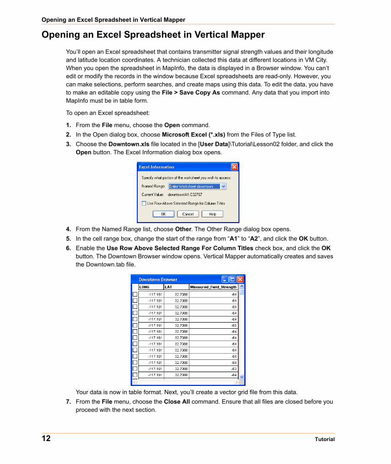
1. From the File menu, choose the Open command.2. In the Open dialog box, choose Microsoft Excel (*.xls) from the Files of Type list.3. Choose the Downtown.xls file located in the [User Data]\Tutorial\Lesson02 folder, and click the
Open button. The Excel Information dialog box opens.
4. From the Named Range list, choose Other. The Other Range dialog box opens.5. In the cell range box, change the start of the range from “A1” to “A2”, and click the OK button.6. Enable the Use Row Above Selected Range For Column Titles check box, and click the OK
button. The Downtown Browser window opens. Vertical Mapper automatically creates and saves the Downtown.tab file.
Your data is now in table format. Next, you’ll create a vector grid file from this data.7. From the File menu, choose the Close All command. Ensure that all files are closed before you
proceed with the next section.
12 Tutorial
Chapter 2: Preparing Data for Analysis
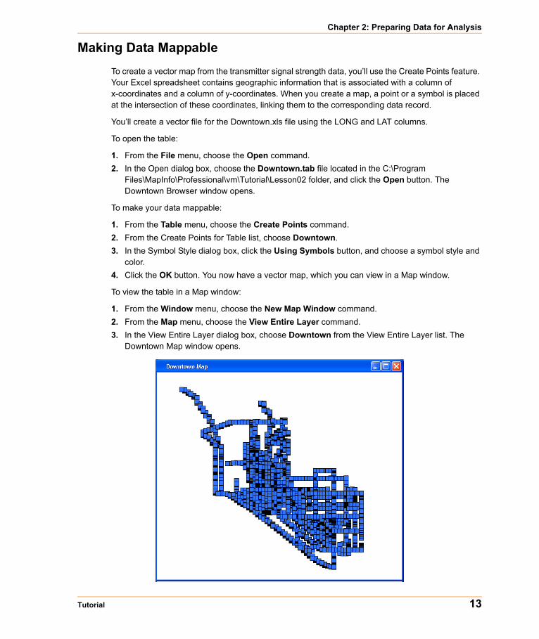
Making Data MappableTo create a vector map from the transmitter signal strength data, you’ll use the Create Points feature. Your Excel spreadsheet contains geographic information that is associated with a column of x-coordinates and a column of y-coordinates. When you create a map, a point or a symbol is placed at the intersection of these coordinates, linking them to the corresponding data record.
You’ll create a vector file for the Downtown.xls file using the LONG and LAT columns.
To open the table:
1. From the File menu, choose the Open command.2. In the Open dialog box, choose the Downtown.tab file located in the C:\Program
Files\MapInfo\Professional\vm\Tutorial\Lesson02 folder, and click the Open button. The Downtown Browser window opens.
To make your data mappable:
1. From the Table menu, choose the Create Points command.2. From the Create Points for Table list, choose Downtown.3. In the Symbol Style dialog box, click the Using Symbols button, and choose a symbol style and
color.4. Click the OK button. You now have a vector map, which you can view in a Map window.
To view the table in a Map window:
1. From the Window menu, choose the New Map Window command.2. From the Map menu, choose the View Entire Layer command.3. In the View Entire Layer dialog box, choose Downtown from the View Entire Layer list. The
Downtown Map window opens.
Tutorial 13

Changing the Native Projection System
Changing the Native Projection SystemThe Downtown.tab file that was created is in degrees longitude and latitude. However, the longitude/latitude coordinate system is not a suitable projection system for graphic presentations because one degree of latitude is not the same distance as one degree of longitude. This difference in distance makes your grid appear visually distorted in a Map window. To avoid this distortion, you’ll reproject the data to a Universal Transverse Mercator (UTM) projection system that uses metres. Any file you process within Vertical Mapper should be in a projection system using distance as the coordinate unit, because many functions in Vertical Mapper require grids with a cartesian unit of measure.
To change the native projection:
1. From the File menu, choose the Save Copy As command.2. In the File name box, change the file name to Downtown_UTM.tab. 3. Click the Projection button.4. From the Category list, choose Universal Transverse Mercator (NAD 83).5. From the Category Member list, choose UTM Zone 10 (NAD 83), and click the OK button.6. Click the Save button. The file is now saved with the UTM projection system.
Aggregating DataData aggregation reduces the number of points in a file. Different methods are available to process the original point file, but all spatially group and statistically average points that are in close proximity and produce a point file with fewer data points. Aggregation also creates a more uniform distribution of points and decreases the time required to generate a grid.
Understanding your Data SetBefore you aggregate your data, it is important to understand why it needs to be aggregated.
The Downtown_UTM data set is typical of the data collected by telecommunication companies when they are measuring the strength of the signal produced by transmitters. Essentially, technicians drive along roadways recording the x- and y-coordinates of the vehicle’s location and the transmitter signal strength at that location. As the vehicle moves and changes speed, the distribution of the sample points changes accordingly. For example, points will be very close or coincident when the vehicle slows or stops.
The Downtown_UTM.tab file contains 32,767 drive test points. Many data points are close together or coincident, making the information carried by these points redundant. Therefore, it is appropriate to aggregate this data before creating a grid.
14 Tutorial

Chapter 2: Preparing Data for Analysis
Aggregating Downtown_UTM.TABBecause the data set is not large enough to make processing time a factor, you’ll aggregate the data using the Cluster Density method.
Before you aggregate the data, you should investigate the data set to determine an appropriate distance to use in the aggregation. The distance you choose is subjective and depends on the data set and the reasons for aggregating. To determine the aggregation distance, zoom-in on the map and, with the Radius Select tool, begin examining the number of points selected at different radius distances. To determine the number of points selected, open the Statistics window.
Although there appear to be only five records in the search radius, there are actually 16 records, as shown in the Statistics dialog box.
In the figure above, a radius of 25 meters was shown to select approximately 15 points in different areas of the map. If this was consistent throughout the whole map, then the resulting point file will contain approximately 2184 points (32 767 / 15). Therefore, an aggregation distance of 25 meters will be used in the lesson because both the aggregation distance and the estimated number of points is reasonable.
To aggregate points:
1. From the Vertical Mapper menu, choose the Data Aggregation > Point Aggregation with Statistics command. The Select Table and Columns dialog box opens.
2. From the Select Table To Aggregate list, choose Downtown_UTM.3. From the Select Column list, choose Measured_Field_Strength, and click the Next button. The
Select Coincident Point Technique dialog box opens.
Tutorial 15
Aggregating Data
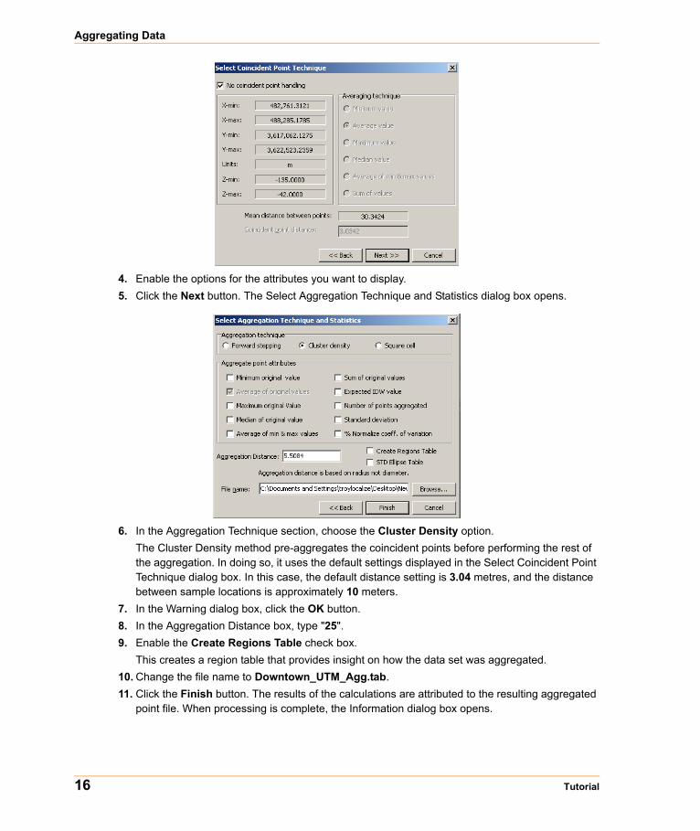
4. Enable the options for the attributes you want to display.5. Click the Next button. The Select Aggregation Technique and Statistics dialog box opens.
6. In the Aggregation Technique section, choose the Cluster Density option.The Cluster Density method pre-aggregates the coincident points before performing the rest of the aggregation. In doing so, it uses the default settings displayed in the Select Coincident Point Technique dialog box. In this case, the default distance setting is 3.04 metres, and the distance between sample locations is approximately 10 meters.
7. In the Warning dialog box, click the OK button.8. In the Aggregation Distance box, type "25".9. Enable the Create Regions Table check box.
This creates a region table that provides insight on how the data set was aggregated.10. Change the file name to Downtown_UTM_Agg.tab. 11. Click the Finish button. The results of the calculations are attributed to the resulting aggregated
point file. When processing is complete, the Information dialog box opens.
16 Tutorial
Chapter 2: Preparing Data for Analysis
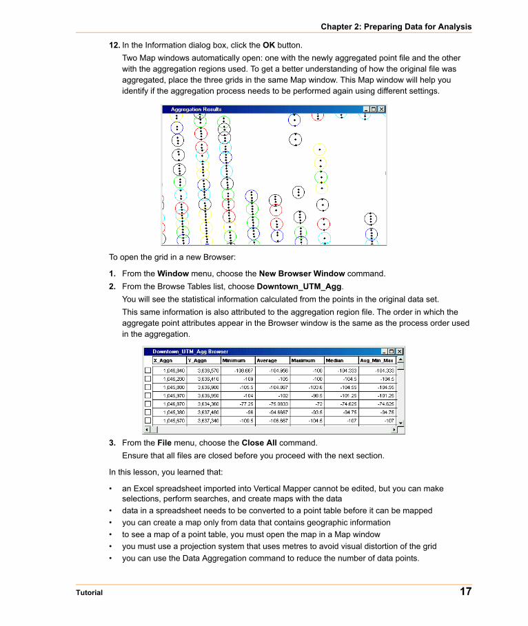
12. In the Information dialog box, click the OK button.Two Map windows automatically open: one with the newly aggregated point file and the other with the aggregation regions used. To get a better understanding of how the original file was aggregated, place the three grids in the same Map window. This Map window will help you identify if the aggregation process needs to be performed again using different settings.
To open the grid in a new Browser:
1. From the Window menu, choose the New Browser Window command.2. From the Browse Tables list, choose Downtown_UTM_Agg.
You will see the statistical information calculated from the points in the original data set. This same information is also attributed to the aggregation region file. The order in which the aggregate point attributes appear in the Browser window is the same as the process order used in the aggregation.
3. From the File menu, choose the Close All command.Ensure that all files are closed before you proceed with the next section.
In this lesson, you learned that:
• an Excel spreadsheet imported into Vertical Mapper cannot be edited, but you can make selections, perform searches, and create maps with the data
• data in a spreadsheet needs to be converted to a point table before it can be mapped• you can create a map only from data that contains geographic information• to see a map of a point table, you must open the map in a Map window• you must use a projection system that uses metres to avoid visual distortion of the grid• you can use the Data Aggregation command to reduce the number of data points.
Tutorial 17

Aggregating Data
18 Tutorial

3
Creating Grids Using Interpolation (Basic)You’ll create a numerical grid from elevation data, which is in a point file, using the Triangular Irregular Network (TIN) interpolation method. Triangulation is usually applied to data that requires no regional averaging, such as elevation data.
You’ll also use the Natural Neighbour Interpolation Method to create a numeric grid from a point file. Natural neighbour interpolation is a geometric estimation technique that uses natural neighbour regions generated around each point in the data. This technique is particularly effective for dealing with spatial data exhibiting clustered or highly linear distributions.
You’ll create a classified grid for the land use data by converting regions to a grid. You’ll also convert elevation data, which is in the form of a contour file, into a point file from which you will then create a numeric grid using the Poly-to-Point function.
In this lesson, you’ll learn:
Creating a Numeric Grid using TIN Interpolation . . . . . . . . . . . . .20Inspecting the Data . . . . . . . . . . . . . . . . . . . . . . . . . . . . . . . . . . . . .23Using the Poly-to-Point Function to Create a Point File. . . . . . . .23Creating a Numeric Grid using Simple Natural Neighbour Interpolation27Creating a Classified Grid . . . . . . . . . . . . . . . . . . . . . . . . . . . . . . . .28
Required files can be found in:• [User Data]\Tutorial\Lesson03 folder
Creating a Numeric Grid using TIN Interpolation
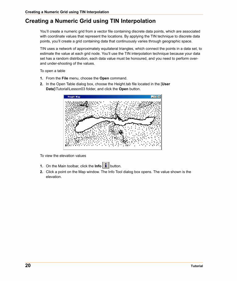
Creating a Numeric Grid using TIN InterpolationYou’ll create a numeric grid from a vector file containing discrete data points, which are associated with coordinate values that represent the locations. By applying the TIN technique to discrete data points, you’ll create a grid containing data that continuously varies through geographic space.
TIN uses a network of approximately equilateral triangles, which connect the points in a data set, to estimate the value at each grid node. You’ll use the TIN interpolation technique because your data set has a random distribution, each data value must be honoured, and you need to perform over- and under-shooting of the values.
To open a table
1. From the File menu, choose the Open command.2. In the Open Table dialog box, choose the Height.tab file located in the [User
Data]\Tutorial\Lesson03 folder, and click the Open button.
To view the elevation values
1. On the Main toolbar, click the Info button.2. Click a point on the Map window. The Info Tool dialog box opens. The value shown is the
elevation.
20 Tutorial
Chapter 3: Creating Grids Using Interpolation (Basic)
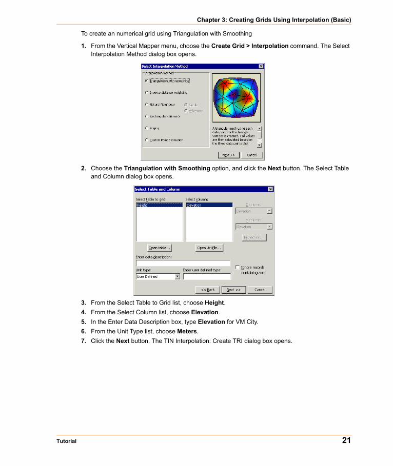
To create an numerical grid using Triangulation with Smoothing
1. From the Vertical Mapper menu, choose the Create Grid > Interpolation command. The Select Interpolation Method dialog box opens.
2. Choose the Triangulation with Smoothing option, and click the Next button. The Select Table and Column dialog box opens.
3. From the Select Table to Grid list, choose Height. 4. From the Select Column list, choose Elevation.5. In the Enter Data Description box, type Elevation for VM City.6. From the Unit Type list, choose Meters.7. Click the Next button. The TIN Interpolation: Create TRI dialog box opens.
Tutorial 21
Creating a Numeric Grid using TIN Interpolation
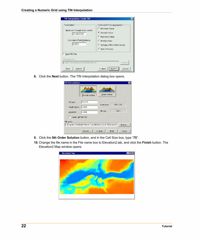
8. Click the Next button. The TIN Interpolation dialog box opens.
9. Click the 5th Order Solution button, and in the Cell Size box, type “75”.10. Change the file name in the File name box to Elevation2.tab, and click the Finish button. The
Elevation2 Map window opens.
22 Tutorial
Chapter 3: Creating Grids Using Interpolation (Basic)
Inspecting the DataNext, you’ll inspect the values around a point using the Grid Info tool.
To inspect the data
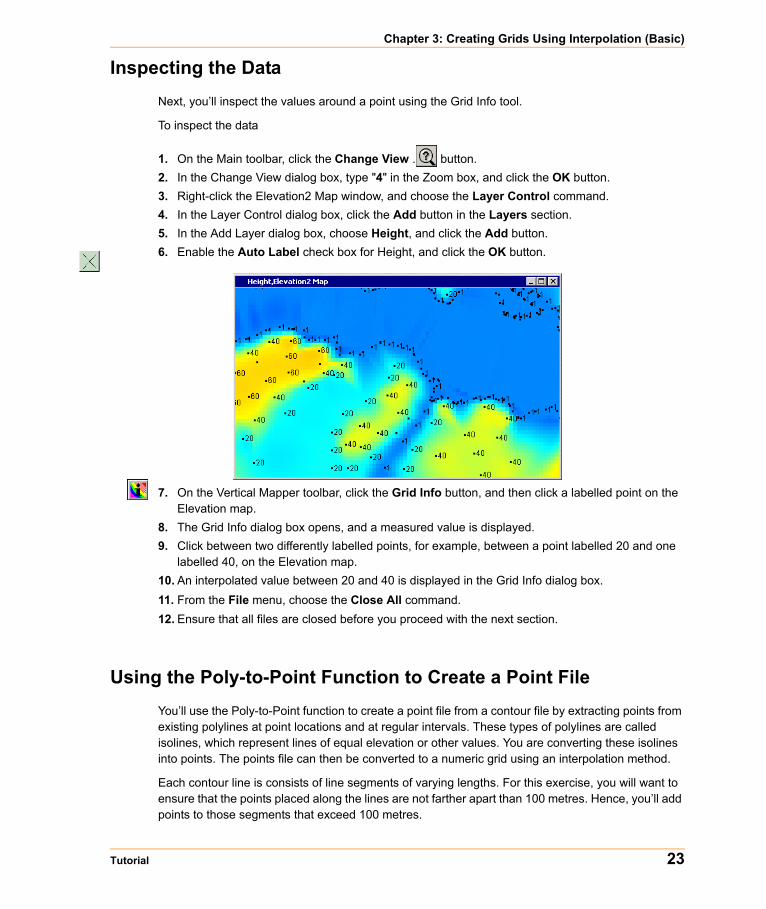
1. On the Main toolbar, click the Change View . button.2. In the Change View dialog box, type "4" in the Zoom box, and click the OK button.3. Right-click the Elevation2 Map window, and choose the Layer Control command.4. In the Layer Control dialog box, click the Add button in the Layers section.5. In the Add Layer dialog box, choose Height, and click the Add button.6. Enable the Auto Label check box for Height, and click the OK button.
7. On the Vertical Mapper toolbar, click the Grid Info button, and then click a labelled point on the Elevation map.
8. The Grid Info dialog box opens, and a measured value is displayed.9. Click between two differently labelled points, for example, between a point labelled 20 and one
labelled 40, on the Elevation map.10. An interpolated value between 20 and 40 is displayed in the Grid Info dialog box.11. From the File menu, choose the Close All command.12. Ensure that all files are closed before you proceed with the next section.
Using the Poly-to-Point Function to Create a Point FileYou’ll use the Poly-to-Point function to create a point file from a contour file by extracting points from existing polylines at point locations and at regular intervals. These types of polylines are called isolines, which represent lines of equal elevation or other values. You are converting these isolines into points. The points file can then be converted to a numeric grid using an interpolation method.
Each contour line is consists of line segments of varying lengths. For this exercise, you will want to ensure that the points placed along the lines are not farther apart than 100 metres. Hence, you’ll add points to those segments that exceed 100 metres.
Tutorial 23
Using the Poly-to-Point Function to Create a Point File
You’ll use the Poly-to-Point function to create a numeric grid when your data is available only as a line or a region object.
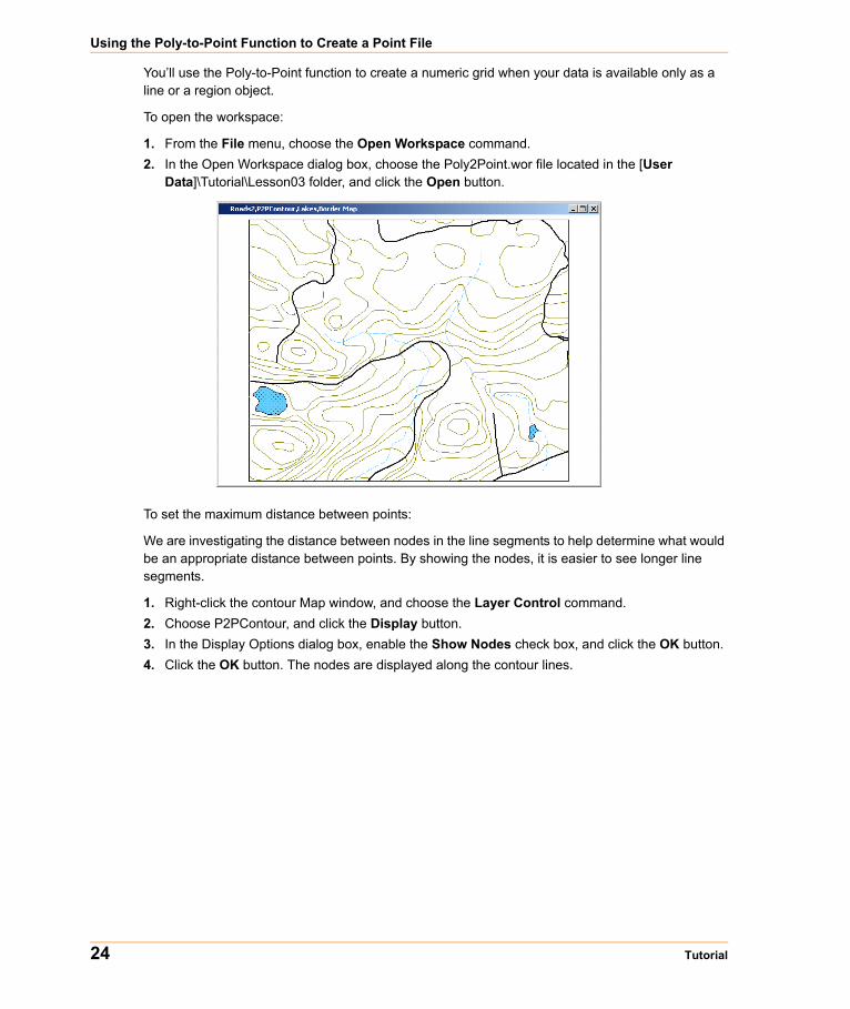
To open the workspace:
1. From the File menu, choose the Open Workspace command.2. In the Open Workspace dialog box, choose the Poly2Point.wor file located in the [User
Data]\Tutorial\Lesson03 folder, and click the Open button.
To set the maximum distance between points:
We are investigating the distance between nodes in the line segments to help determine what would be an appropriate distance between points. By showing the nodes, it is easier to see longer line segments.
1. Right-click the contour Map window, and choose the Layer Control command.2. Choose P2PContour, and click the Display button.3. In the Display Options dialog box, enable the Show Nodes check box, and click the OK button. 4. Click the OK button. The nodes are displayed along the contour lines.
24 Tutorial

Chapter 3: Creating Grids Using Interpolation (Basic)
5. On the Main toolbar, click the Zoom-in button, and click on a long line segment.6. From the Map menu, choose the Options command.7. From the Distance Units list, choose kilometers, and click the OK button.
8. On the Main toolbar, click the Ruler button.9. Click the first node of the long line segment, and then click the second node.
The length of the line segment is displayed in the Ruler dialog box. This line segment exceeds 100 metres. Therefore, you’ll have add nodes to this and other line segments so that this contour is better defined when the grid is created.
10. From the Vertical Mapper menu, choose the Create Grid > Poly-to-Point command. The Poly-to-Point dialog box opens.
11. From the Select Table list, choose P2PContour.12. In the Extract From section, enable the Polylines check box. 13. Choose the Set Maximum option, and type “100” in the Distance box.
Tutorial 25
Using the Poly-to-Point Function to Create a Point File
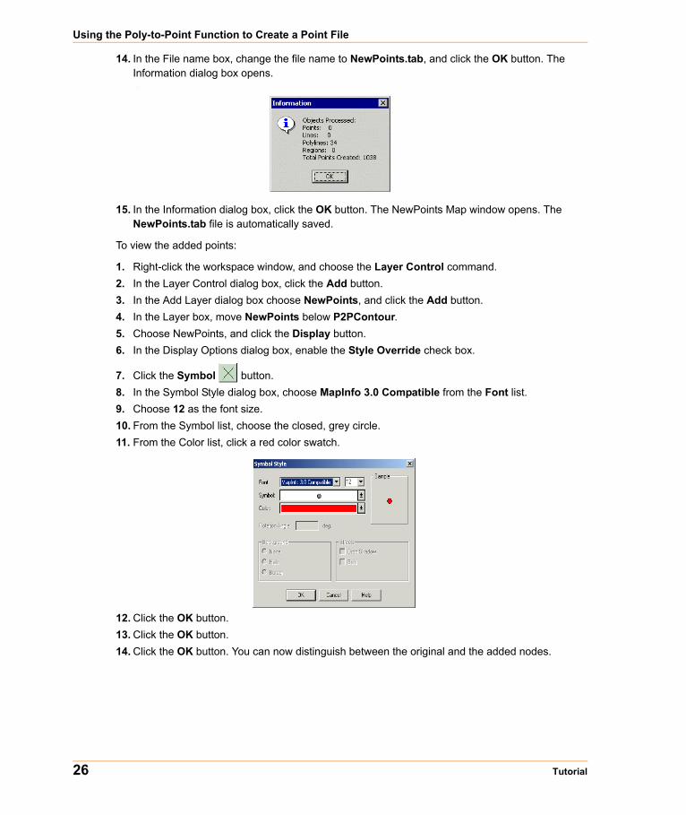
14. In the File name box, change the file name to NewPoints.tab, and click the OK button. The Information dialog box opens.
.
15. In the Information dialog box, click the OK button. The NewPoints Map window opens. The NewPoints.tab file is automatically saved.
To view the added points:
1. Right-click the workspace window, and choose the Layer Control command.2. In the Layer Control dialog box, click the Add button.3. In the Add Layer dialog box choose NewPoints, and click the Add button.4. In the Layer box, move NewPoints below P2PContour.5. Choose NewPoints, and click the Display button. 6. In the Display Options dialog box, enable the Style Override check box.
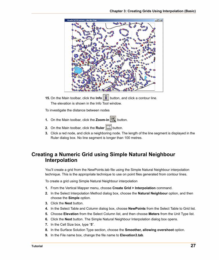
7. Click the Symbol button.8. In the Symbol Style dialog box, choose MapInfo 3.0 Compatible from the Font list.9. Choose 12 as the font size.10. From the Symbol list, choose the closed, grey circle.11. From the Color list, click a red color swatch.
12. Click the OK button.13. Click the OK button.14. Click the OK button. You can now distinguish between the original and the added nodes.
26 Tutorial
Chapter 3: Creating Grids Using Interpolation (Basic)
15. On the Main toolbar, click the Info button, and click a contour line.The elevation is shown in the Info Tool window.
To investigate the distance between nodes
1. On the Main toolbar, click the Zoom-in button.
2. On the Main toolbar, click the Ruler button.3. Click a red node, and click a neighboring node. The length of the line segment is displayed in the
Ruler dialog box. No line segment is longer than 100 metres.
Creating a Numeric Grid using Simple Natural Neighbour InterpolationYou’ll create a grid from the NewPoints.tab file using the Simple Natural Neighbour interpolation technique. This is the appropriate technique to use on point files generated from contour lines.
To create a grid using Simple Natural Neighbour interpolation
1. From the Vertical Mapper menu, choose Create Grid > Interpolation command.2. In the Select Interpolation Method dialog box, choose the Natural Neighbour option, and then
choose the Simple option.3. Click the Next button. 4. In the Select Table and Column dialog box, choose NewPoints from the Select Table to Grid list.5. Choose Elevation from the Select Column list, and then choose Meters from the Unit Type list. 6. Click the Next button. The Simple Natural Neighbour Interpolation dialog box opens.7. In the Cell Size box, type “5”.8. In the Surface Solution Type section, choose the Smoother, allowing overshoot option.9. In the File name box, change the file name to Elevation3.tab.
Tutorial 27
Creating a Classified Grid
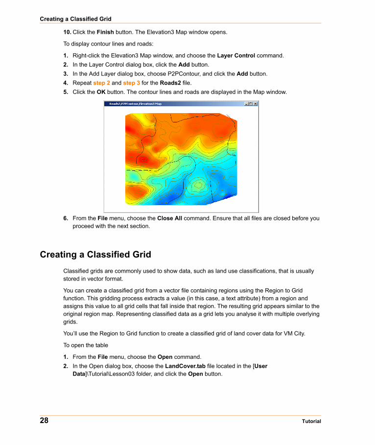
10. Click the Finish button. The Elevation3 Map window opens.
To display contour lines and roads:
1. Right-click the Elevation3 Map window, and choose the Layer Control command.2. In the Layer Control dialog box, click the Add button.3. In the Add Layer dialog box, choose P2PContour, and click the Add button. 4. Repeat step 2 and step 3 for the Roads2 file.5. Click the OK button. The contour lines and roads are displayed in the Map window.
6. From the File menu, choose the Close All command. Ensure that all files are closed before you proceed with the next section.
Creating a Classified GridClassified grids are commonly used to show data, such as land use classifications, that is usually stored in vector format.
You can create a classified grid from a vector file containing regions using the Region to Grid function. This gridding process extracts a value (in this case, a text attribute) from a region and assigns this value to all grid cells that fall inside that region. The resulting grid appears similar to the original region map. Representing classified data as a grid lets you analyse it with multiple overlying grids.
You’ll use the Region to Grid function to create a classified grid of land cover data for VM City.
To open the table
1. From the File menu, choose the Open command.2. In the Open dialog box, choose the LandCover.tab file located in the [User
Data]\Tutorial\Lesson03 folder, and click the Open button.
28 Tutorial
Chapter 3: Creating Grids Using Interpolation (Basic)
To create a classified grid:
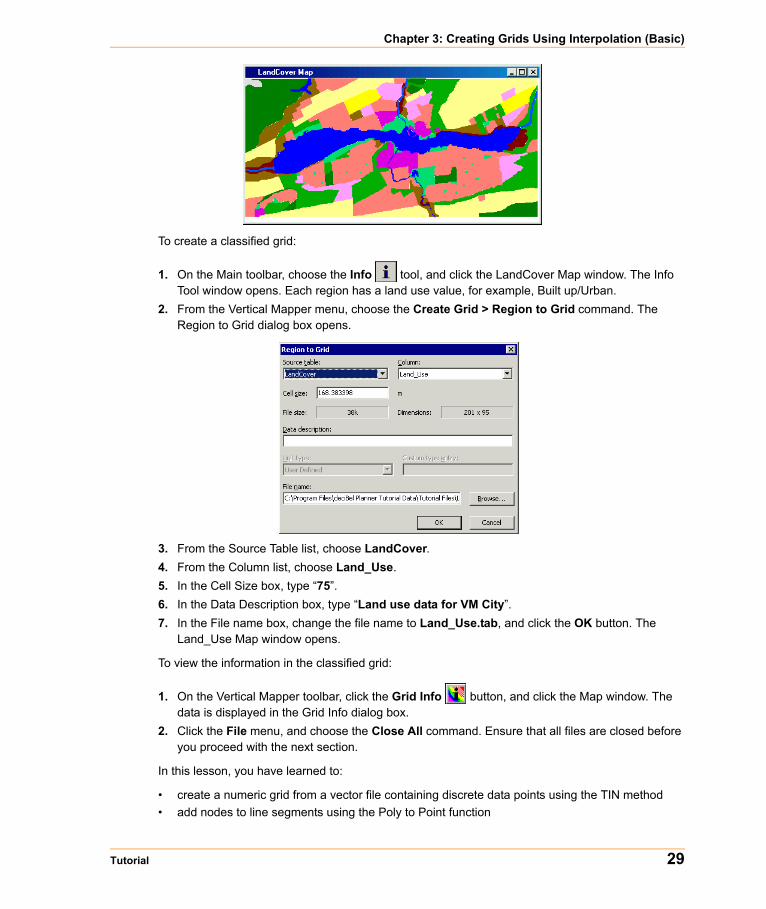
1. On the Main toolbar, choose the Info tool, and click the LandCover Map window. The Info Tool window opens. Each region has a land use value, for example, Built up/Urban.
2. From the Vertical Mapper menu, choose the Create Grid > Region to Grid command. The Region to Grid dialog box opens.
3. From the Source Table list, choose LandCover.4. From the Column list, choose Land_Use.5. In the Cell Size box, type “75”.6. In the Data Description box, type “Land use data for VM City”. 7. In the File name box, change the file name to Land_Use.tab, and click the OK button. The
Land_Use Map window opens.
To view the information in the classified grid:
1. On the Vertical Mapper toolbar, click the Grid Info button, and click the Map window. The data is displayed in the Grid Info dialog box.
2. Click the File menu, and choose the Close All command. Ensure that all files are closed before you proceed with the next section.
In this lesson, you have learned to:
• create a numeric grid from a vector file containing discrete data points using the TIN method• add nodes to line segments using the Poly to Point function
Tutorial 29

Creating a Classified Grid
• create a numeric grid using the Simple Natural Neighbour interpolation• create a classified grid from a vector file using the Region to Grid function
30 Tutorial

4
Creating Grids using Interpolation (Advanced)Inverse Distance Weighting (IDW) interpolation is a moving average interpolation technique that is usually applied to highly variable data. For certain data types, it is possible to return to the collection site and record a new value that is statistically different from the original reading but within the general trend for the area. Examples of this type of data include environmental monitoring data such as soil chemistry and consumer behaviour observations. It is not desirable to honour local high/low values but rather to look at a moving average of nearby data points and estimate the local trends.
Rectangular interpolation is usually applied to data that is regularly and closely spaced, such as points generated from another gridding application. This technique creates an interpolation surface that passes through all points without overshooting the maximum values or undershooting the minimum values.
In this lesson, you’ll learn how to
Creating a Grid using Inverse Distance Weighting Interpolation, p. 32Creating a Numeric Grid using Rectangular Interpolation. . . . . .35
Required files can be found in:• [User Data]\Tutorial\Lesson04 folder
Creating a Grid using Inverse Distance Weighting Interpolation
Creating a Grid using Inverse Distance Weighting InterpolationYou’ll use the IDW interpolation technique to create a numeric grid from a point file. The IDW technique estimates the value of each grid node by averaging all the data points that fall within a given distance. The averaging calculation weights the value at each point, so that the farther a point lies from the grid node, the less influence it exerts.
In this exercise, you’ll interpolate a surface of radioactivity for soil samples taken around a fictional nuclear power plant. The IDW technique is suitable when values are highly variable and when it is impractical to honour each data point.
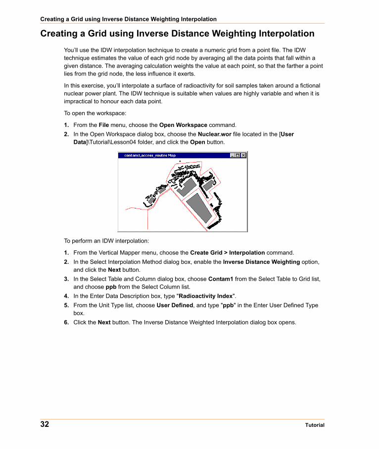
To open the workspace:
1. From the File menu, choose the Open Workspace command.2. In the Open Workspace dialog box, choose the Nuclear.wor file located in the [User
Data]\Tutorial\Lesson04 folder, and click the Open button.
To perform an IDW interpolation:
1. From the Vertical Mapper menu, choose the Create Grid > Interpolation command.2. In the Select Interpolation Method dialog box, enable the Inverse Distance Weighting option,
and click the Next button.3. In the Select Table and Column dialog box, choose Contam1 from the Select Table to Grid list,
and choose ppb from the Select Column list.4. In the Enter Data Description box, type "Radioactivity Index".5. From the Unit Type list, choose User Defined, and type "ppb" in the Enter User Defined Type
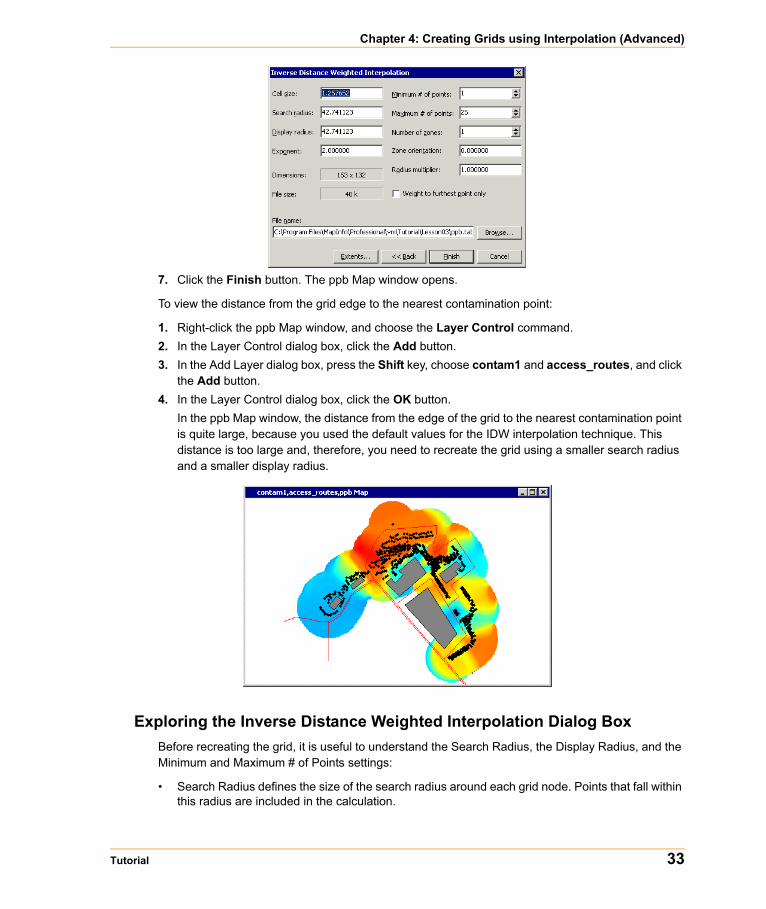
box.6. Click the Next button. The Inverse Distance Weighted Interpolation dialog box opens.
32 Tutorial
Chapter 4: Creating Grids using Interpolation (Advanced)
7. Click the Finish button. The ppb Map window opens.
To view the distance from the grid edge to the nearest contamination point:
1. Right-click the ppb Map window, and choose the Layer Control command.2. In the Layer Control dialog box, click the Add button.3. In the Add Layer dialog box, press the Shift key, choose contam1 and access_routes, and click
the Add button.4. In the Layer Control dialog box, click the OK button.
In the ppb Map window, the distance from the edge of the grid to the nearest contamination point is quite large, because you used the default values for the IDW interpolation technique. This distance is too large and, therefore, you need to recreate the grid using a smaller search radius and a smaller display radius.
Exploring the Inverse Distance Weighted Interpolation Dialog BoxBefore recreating the grid, it is useful to understand the Search Radius, the Display Radius, and the Minimum and Maximum # of Points settings:
• Search Radius defines the size of the search radius around each grid node. Points that fall within this radius are included in the calculation.
Tutorial 33

Creating a Grid using Inverse Distance Weighting Interpolation
• Display Radius defines the circular radius around each grid node that predetermines the number of points to include in the calculation. The Display Radius controls the distance beyond which the grid will be created.
• Minimum and Maximum # of Points defines the minimum number of points that fall inside the Display Radius for a grid node to get a calculated value and the maximum number of points that will be used in the calculation.
To determine the values for the search and the display radius:
1. On the Main toolbar, click the Zoom-in button, and then click near the edge of the grid.2. From the Map menu, choose the Options command.3. In the Map Options dialog box, choose meters from the Distance Units list, and click the OK
button.
4. On the Main toolbar, click the Ruler button, click the edge of the grid, and then click a point.The distance between the edge and a point is around 44 metres. A distance of 25 metres is more suitable. When you choose a new distance, keep the following in mind:a. How many points do you want to use in the averaging calculation?b. How big are the gaps and do you wish to interpolate values there?c. How far beyond the limits of the point file would you like the grid surface to be created?As a general rule for most data sets, it is appropriate to have the same distance for the Search Radius and for the Display Radius.
To re-interpolate using the IDW technique:
1. From the Vertical Mapper menu, choose the Create Grid > Interpolation command.2. In the Select Interpolation Method dialog box, choose the Inverse Distance Weighting option,
and click the Next button.3. In the Select Table and Column dialog box, choose Contam1 from the Select Table to Grid list,
and then choose ppb from the Select Column list.4. In the Enter Data Description box, type "Radioactivity Index".5. From the Unit Type list, choose User Defined, and type "ppb" in the Enter User Defined Type
box.6. Click the Next button. The Inverse Distance Weighted Interpolation dialog box opens.7. Type "2" in the Cell Size box.8. Type "25" in the Search Radius box.9. Type "25" in the Display Radius box.10. Type "2" in the Minimum # of Points box.11. Change the file name to ppb2.tab, and click the Finish button. The ppb2 Map window opens.
34 Tutorial

Chapter 4: Creating Grids using Interpolation (Advanced)
From the resulting surface, it looks as if there are several areas of relatively high radioactivity. However, this may not be the case in reality, and it may be necessary to change the colour scheme, so that the truly high values of radioactivity are coloured red.
To load a new colour profile:
1. In the Grid Manager, click the Colour button. The Grid Colour Tool dialog box opens.2. In the Colour Profile section, click the Load button.3. In the Open dialog box, choose the Nuclear.vcp file located in the [User
Data]\Tutorial\Lesson04 folder, and click the Open button.4. In the Grid Colour Tool dialog box, click the OK button. The locations of high radioactivity are
coloured red, and those of low are coloured blue.5. From the File menu, choose the Close All command. Ensure that all files are closed before you
proceed with the next section.
Creating a Numeric Grid using Rectangular InterpolationThe Rectangular Interpolation technique estimates a grid by creating a circular radius around each grid node. This radius is then divided into four equal quadrants from which the closest data point in each is selected. It is from these four points that the new grid node value is calculated. In this exercise, you’ll create an elevation surface from a point file with regularly spaced elevation values. The file used in this exercise was exported to a MapInfo point file. The site is in Olympic National Park, Washington, United States.
You will use the Rectangular Interpolation technique because the data is regularly spaced, and you do need to honour every data value. You area assuming that over/undershooting of the data values was performed in the software program in which the file was created.
To open the table:
1. From the File menu, choose the Open command.2. In the Open Table dialog box, choose the Rectangular.tab file located in [User
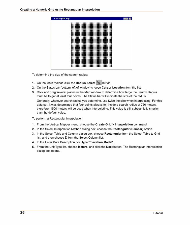
Data]\Tutorial\Lesson04 folder, and click the Open button. The distribution of the points is very regular, which makes this data ideal for interpolation using the Rectangular Interpolation method.
Tutorial 35
Creating a Numeric Grid using Rectangular Interpolation
To determine the size of the search radius:
1. On the Main toolbar, click the Radius Select button.2. On the Status bar (bottom left of window) choose Cursor Location from the list.3. Click and drag several places in the Map window to determine how large the Search Radius
must be to get at least four points. The Status bar will indicate the size of the radius.Generally, whatever search radius you determine, use twice the size when interpolating. For this data set, it was determined that four points always fell inside a search radius of 750 meters, therefore, 1500 meters will be used when interpolating. This value is still substantially smaller than the default value.
To perform a Rectangular interpolation:
1. From the Vertical Mapper menu, choose the Create Grid > Interpolation command.2. In the Select Interpolation Method dialog box, choose the Rectangular (Bilinear) option.3. In the Select Table and Column dialog box, choose Rectangular from the Select Table to Grid
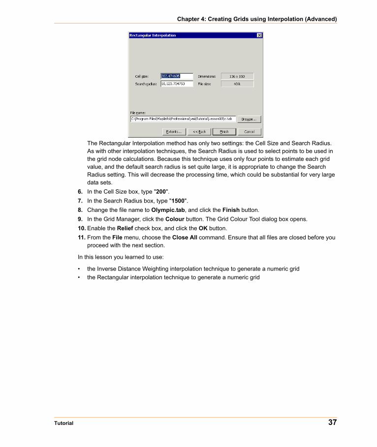
list, and then choose Z from the Select Column list.4. In the Enter Data Description box, type "Elevation Model".5. From the Unit Type list, choose Meters, and click the Next button. The Rectangular Interpolation
dialog box opens.
36 Tutorial
Chapter 4: Creating Grids using Interpolation (Advanced)
The Rectangular Interpolation method has only two settings: the Cell Size and Search Radius. As with other interpolation techniques, the Search Radius is used to select points to be used in the grid node calculations. Because this technique uses only four points to estimate each grid value, and the default search radius is set quite large, it is appropriate to change the Search Radius setting. This will decrease the processing time, which could be substantial for very large data sets.
6. In the Cell Size box, type "200".7. In the Search Radius box, type "1500".8. Change the file name to Olympic.tab, and click the Finish button.9. In the Grid Manager, click the Colour button. The Grid Colour Tool dialog box opens.10. Enable the Relief check box, and click the OK button.11. From the File menu, choose the Close All command. Ensure that all files are closed before you
proceed with the next section.
In this lesson you learned to use:
• the Inverse Distance Weighting interpolation technique to generate a numeric grid• the Rectangular interpolation technique to generate a numeric grid
Tutorial 37

Creating a Numeric Grid using Rectangular Interpolation
38 Tutorial
5
Creating Grids Using Spatial ModellingIn the first part of this lesson, you’ll determine the proposed location of one or more new delivery hubs for a messenger service operating in the VM City area. This will be accomplished by analyzing the current distribution of customers while taking into account the usage frequency for each customer. A map has been created that shows the location of all the customers who have used the service at least once a month in the past year. The frequency-of-use data is presented in the customer point table. Ideally, you would like to limit the travel distance of your delivery trucks to five kilometers. Presently, the delivery hub is located in the downtown core.
In the second part of the lesson, your friend, who is the owner of an ice cream store chain, is planning to open stores in VM City. You’ll perform an analysis on his existing stores to help him determine possible new locations. Through extensive research, you have determined the attractiveness value for all the competing businesses and determined that a person will not walk more than 1000 metres for a scoop of ice cream. You’ll need to perform the analysis twice; in the first analysis, a trade area will be calculated for an individual site, and in the second, trade areas will be calculated for competing stores.
In this lesson, you’ll learn:
Modeling using the Location Profiler . . . . . . . . . . . . . . . . . . . . . . .40Modeling with Trade Area Analysis . . . . . . . . . . . . . . . . . . . . . . . .41Calculating the Maximum Patronage for All Sites . . . . . . . . . . . .43
Required files can be found in:• [User Data]\Tutorial\Lesson05 folder
Modeling using the Location Profiler
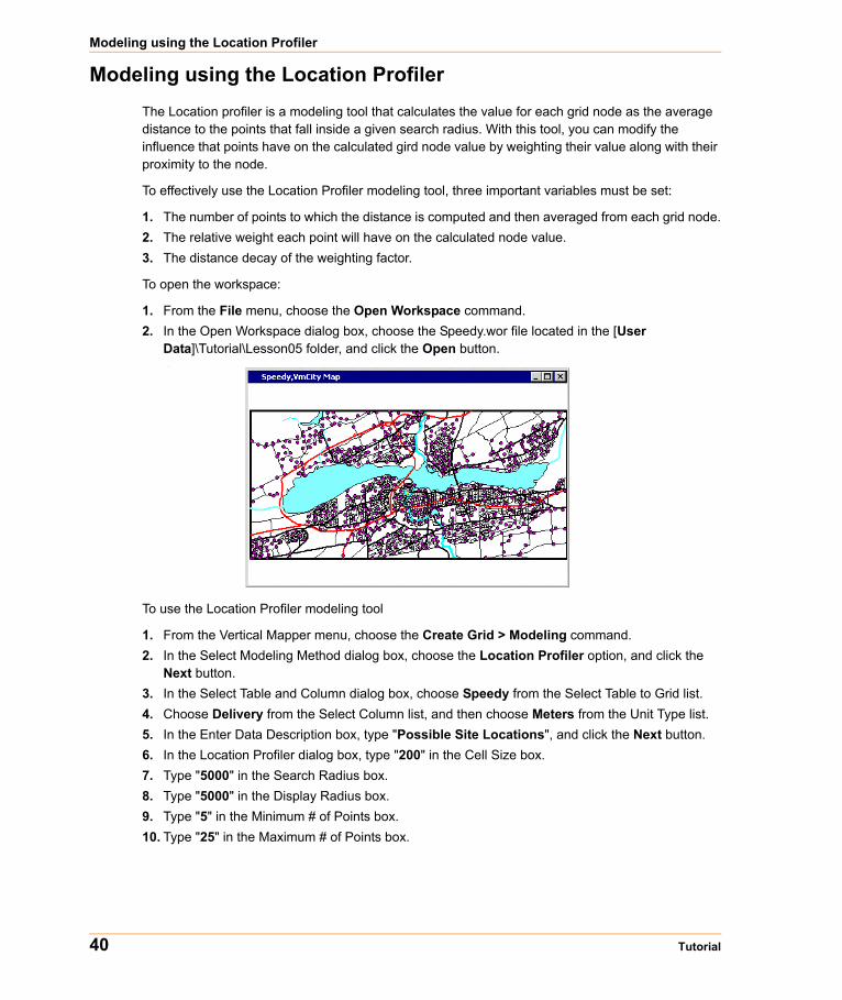
Modeling using the Location ProfilerThe Location profiler is a modeling tool that calculates the value for each grid node as the average distance to the points that fall inside a given search radius. With this tool, you can modify the influence that points have on the calculated gird node value by weighting their value along with their proximity to the node.
To effectively use the Location Profiler modeling tool, three important variables must be set:
1. The number of points to which the distance is computed and then averaged from each grid node.2. The relative weight each point will have on the calculated node value.3. The distance decay of the weighting factor.
To open the workspace:
1. From the File menu, choose the Open Workspace command.2. In the Open Workspace dialog box, choose the Speedy.wor file located in the [User
Data]\Tutorial\Lesson05 folder, and click the Open button..
To use the Location Profiler modeling tool
1. From the Vertical Mapper menu, choose the Create Grid > Modeling command.2. In the Select Modeling Method dialog box, choose the Location Profiler option, and click the
Next button.3. In the Select Table and Column dialog box, choose Speedy from the Select Table to Grid list.4. Choose Delivery from the Select Column list, and then choose Meters from the Unit Type list. 5. In the Enter Data Description box, type "Possible Site Locations", and click the Next button.6. In the Location Profiler dialog box, type "200" in the Cell Size box.7. Type "5000" in the Search Radius box.8. Type "5000" in the Display Radius box.9. Type "5" in the Minimum # of Points box.10. Type "25" in the Maximum # of Points box.
40 Tutorial

Chapter 5: Creating Grids Using Spatial Modelling
11. Change the file name to Delivery.tab, and click the Finish button.The Delivery Map window opens. Blue colours indicate low activity, and red colours indicate high activity. This colour pattern is the default colour profile in Vertical Mapper, where high values are assigned hot (red) colours and low values are assigned cold (blue) colors. However, in this example, the areas of interest are the lower values, that is, shorter average distances between the data points. Therefore, the color scheme should be reversed.
To reverse the colour profile of the grid:
1. In the Grid Manager, choose Delivery.grd, and click the Colour button.2. In the Grid Colour Tool dialog box, click the Flip Colour button. The resulting grid shows several
centres of activity, any one of which could potentially be the location of a new delivery hub. You can highlight the centres of activity more dramatically by modifying the colour inflection points at the lower end of the value range.
3. Load the delivery.vcp file located in the C:\Program Files\MapInfo\Professional\vm \Tutorial \Lesson05 folder.
4. From the File menu, choose the Close All command. Ensure that all files are closed before you proceed with the next section.
Modeling with Trade Area AnalysisThe Trade Area Analysis modeling tool generates a patronage probability surface for one or more store locations. Two variables are used when generating this surface. The first is a store’s qualities that make it more or less appealing to a customer (its attractiveness). The second is the spatial distribution of the stores, that is, the distances between stores and each store’s potential customers (grid nodes). In essence, what this modeling tool is doing is calculating trade areas around one or more stores that are more or less likely to be patronized by customers.
The attractiveness of a store is a predetermined value attributed to each store used in the analysis. The value is determined by rating many different qualitative and quantitative characteristics for each store. For example, the amount of floor space, how clean the store is, the number of parking spaces, the age of the store, and the quality of customer service are all factors that could be used to help in defining a store’s appeal.
Calculating the Probable Trade Area for One SiteWhen calculating the trade area for a site, you are evaluating how that location competes with every other store location. In this example, you have the opportunity to take over an existing store location and to determine how that location competes based on an attractiveness value.
To open the workspace
1. From the File menu, choose the Open Workspace command.2. In the Open Workspace dialog box, choose the IceCream.wor file located in the C:\Program
Files\MapInfo\Professional\vm\Tutorial\Lesson05 folder.Each ice cream store has an attractiveness value, as shown on the map.
Tutorial 41

Modeling with Trade Area Analysis
To calculate the probable trade area
1. From the Vertical Mapper menu, choose the Create Grid > Modeling command.2. In the Select Modeling Method dialog box, choose the Trade Area Analysis option, choose the
Single Site option, and click the Next button.3. In the Select Table and Column dialog box, choose IceCream from the Select Table to Grid list,
and then choose Attractiveness from the Attractiveness Column list.4. Type "Patronage for one store" in the Enter Data Description box, and click the Next button.
The Huff Model dialog box opens.
5. In the Huff Model dialog box, type "25" in the Cell Size box, and then type "1000" in the Display Radius box.
6. In the File Name box, change the file name to OneStore.tab, and click the Finish button.7. Choose store location 5 from the Map window when prompted.
42 Tutorial
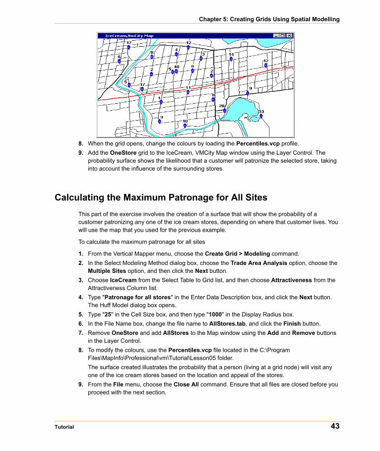
Chapter 5: Creating Grids Using Spatial Modelling
8. When the grid opens, change the colours by loading the Percentiles.vcp profile.9. Add the OneStore grid to the IceCream, VMCity Map window using the Layer Control. The
probability surface shows the likelihood that a customer will patronize the selected store, taking into account the influence of the surrounding stores.
Calculating the Maximum Patronage for All SitesThis part of the exercise involves the creation of a surface that will show the probability of a customer patronizing any one of the ice cream stores, depending on where that customer lives. You will use the map that you used for the previous example.
To calculate the maximum patronage for all sites
1. From the Vertical Mapper menu, choose the Create Grid > Modeling command.2. In the Select Modeling Method dialog box, choose the Trade Area Analysis option, choose the
Multiple Sites option, and then click the Next button.3. Choose IceCream from the Select Table to Grid list, and then choose Attractiveness from the
Attractiveness Column list. 4. Type "Patronage for all stores" in the Enter Data Description box, and click the Next button.
The Huff Model dialog box opens.5. Type "25" in the Cell Size box, and then type "1000" in the Display Radius box.6. In the File Name box, change the file name to AllStores.tab, and click the Finish button.7. Remove OneStore and add AllStores to the Map window using the Add and Remove buttons
in the Layer Control. 8. To modify the colours, use the Percentiles.vcp file located in the C:\Program
Files\MapInfo\Professional\vm\Tutorial\Lesson05 folder.The surface created illustrates the probability that a person (living at a grid node) will visit any one of the ice cream stores based on the location and appeal of the stores.
9. From the File menu, choose the Close All command. Ensure that all files are closed before you proceed with the next section.
Tutorial 43

Calculating the Maximum Patronage for All Sites
In this lesson, you learned that you can:
• use the Location Profiler to determine areas of high and low trade activity• calculate a probable trade area using the Create Grid, Modeling command• calculate a probable trade area for a single site and for Modeling multiple sites
44 Tutorial

6
Creating Cross SectionsUsing the Cross Section tool, you can draw or choose a MapInfo line object that overlies a height grid of the area to construct a vertical profile of elevation along this line.
You are a telecommunications operator who needs to determine where to position his signal relay towers in VM City. In a map window, you’ll generate a vertical profile of the terrain between two potential sites for relay towers to determine if the terrain impedes with the line of sight between these towers. You’ll also generate a vertical profile of the terrain along a line object on the map to see if there is any obstruction to the line of sight.
Finally, you’ll graphically determine the variation in transmitter signal strength with elevation changes along a geographical feature.
In this lesson, you’ll learn how to:
Creating a Cross Section Graph along a Virtual Line. . . . . . . . . .46Customizing a Cross Section Graph . . . . . . . . . . . . . . . . . . . . . . .47Creating a Cross Section Graph from a Line Object . . . . . . . . . .48Showing Elevation and Field Strength along a Line Object. . . . .49
Required files can be found in:• [User Data]\Tutorial\Lesson06 folder

Creating a Cross Section Graph along a Virtual Line
Creating a Cross Section Graph along a Virtual LineYou’ll perform a cross section analysis using the Cross Section tool to determine the location and the height of obstructions along a virtual line between two transmitters. Vertical Mapper samples at regular intervals along the line between those points and records the distance at each interval and the value at that point. In this case, you’ll create a distance versus elevation plot.
To open the workspace:
1. From the File menu, choose the Open Workspace command.2. Choose the CrossSection.wor file located in the [User Data]\Tutorial\Lesson06 folder, and click
the Open button.
To create a cross section:
1. Maximize the Workspace window.
2. On the Vertical Mapper toolbar, click the Cross Section button.3. Position the cursor over the Workspace window. The cursor icon changes into a crosshair.4. Click in the upper-left corner of the map, drag to the lower-right corner, and then double-click.
The Cross Section dialog box opens, showing the height of obstructions between the two points. No points along the line are higher than either of the transmitters.
46 Tutorial
Chapter 6: Creating Cross Sections
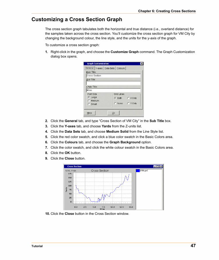
Customizing a Cross Section GraphThe cross section graph tabulates both the horizontal and true distance (i.e., overland distance) for the samples taken across the cross section. You’ll customize the cross section graph for VM City by changing the background colour, the line style, and the units for the y-axis of the graph.
To customize a cross section graph:
1. Right-click in the graph, and choose the Customize Graph command. The Graph Customization dialog box opens.
2. Click the General tab, and type “Cross Section of VM City” in the Sub Title box.3. Click the Y-axes tab, and choose Yards from the Z-units list.4. Click the Data Sets tab, and choose Medium Solid from the Line Style list. 5. Click the red color swatch, and click a blue color swatch in the Basic Colors area.6. Click the Colours tab, and choose the Graph Background option.7. Click the color swatch, and click the white colour swatch in the Basic Colors area.8. Click the OK button.9. Click the Close button.
10. Click the Close button in the Cross Section window.
Tutorial 47
Creating a Cross Section Graph from a Line Object
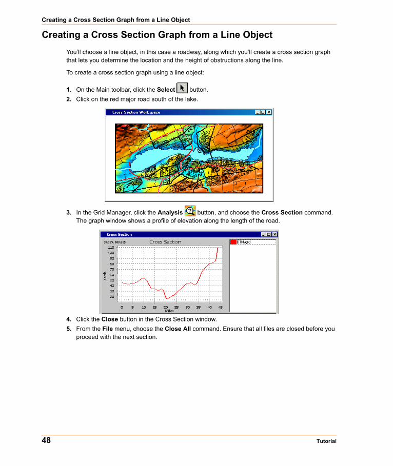
Creating a Cross Section Graph from a Line ObjectYou’ll choose a line object, in this case a roadway, along which you’ll create a cross section graph that lets you determine the location and the height of obstructions along the line.
To create a cross section graph using a line object:
1. On the Main toolbar, click the Select button.2. Click on the red major road south of the lake.
3. In the Grid Manager, click the Analysis button, and choose the Cross Section command. The graph window shows a profile of elevation along the length of the road.
4. Click the Close button in the Cross Section window.5. From the File menu, choose the Close All command. Ensure that all files are closed before you
proceed with the next section.
48 Tutorial
Chapter 6: Creating Cross Sections
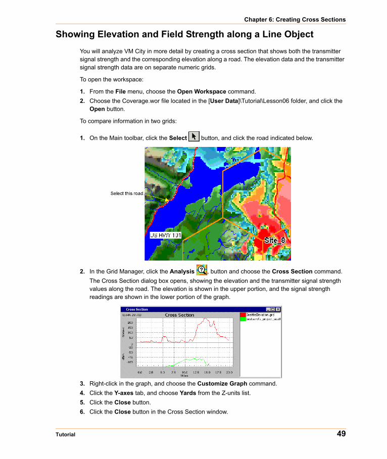
Showing Elevation and Field Strength along a Line ObjectYou will analyze VM City in more detail by creating a cross section that shows both the transmitter signal strength and the corresponding elevation along a road. The elevation data and the transmitter signal strength data are on separate numeric grids.
To open the workspace:
1. From the File menu, choose the Open Workspace command.2. Choose the Coverage.wor file located in the [User Data]\Tutorial\Lesson06 folder, and click the
Open button.
To compare information in two grids:
1. On the Main toolbar, click the Select button, and click the road indicated below.
2. In the Grid Manager, click the Analysis , button and choose the Cross Section command.The Cross Section dialog box opens, showing the elevation and the transmitter signal strength values along the road. The elevation is shown in the upper portion, and the signal strength readings are shown in the lower portion of the graph.
3. Right-click in the graph, and choose the Customize Graph command.4. Click the Y-axes tab, and choose Yards from the Z-units list.5. Click the Close button.6. Click the Close button in the Cross Section window.
Tutorial 49

Showing Elevation and Field Strength along a Line Object
7. From the File menu, choose the Close All command. Ensure that all files are closed before you proceed with the next section.
In this lesson, you learned to:
• use the Cross Section tool to draw a virtual line of sight between two points and view the changes in elevation between these points
• use the Cross Section function on the Surface Analysis toolbar to create a cross section graph along the virtual line to show the location and height of obstruction along the virtual line
• customize the look of a cross section graph• create a cross section graph from a line object on a map• create a cross section graph for two superimposed numeric grids, in this case elevation and
transmitter signal strength grids
50 Tutorial

7
Contouring GridsYou’ve been asked to add contour lines to a numeric and a classified grid. Contour lines are paths of constant value on a grid. The contouring feature generates lines or regions at specified values or at a specified range of values.
In this lesson, you’ll learn:
Creating Line Contours from a Numeric Grid . . . . . . . . . . . . . . . .52Creating Region Contours from a Numeric Grid. . . . . . . . . . . . . .54Contouring a Classified Grid. . . . . . . . . . . . . . . . . . . . . . . . . . . . . .55
Required files can be found in:• [User Data]\Tutorial\Lesson07 folder
Creating Line Contours from a Numeric Grid
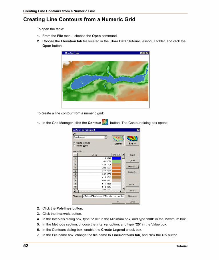
Creating Line Contours from a Numeric GridTo open the table:
1. From the File menu, choose the Open command.2. Choose the Elevation.tab file located in the [User Data]\Tutorial\Lesson07 folder, and click the
Open button.
To create a line contour from a numeric grid:
1. In the Grid Manager, click the Contour . button. The Contour dialog box opens.
2. Click the Polylines button.3. Click the Intervals button.4. In the Intervals dialog box, type "-100" in the Minimum box, and type "800" in the Maximum box. 5. In the Methods section, choose the Interval option, and type "25" in the Value box.6. In the Contours dialog box, enable the Create Legend check box.7. In the File name box, change the file name to LineContours.tab, and click the OK button.
52 Tutorial
Chapter 7: Contouring Grids
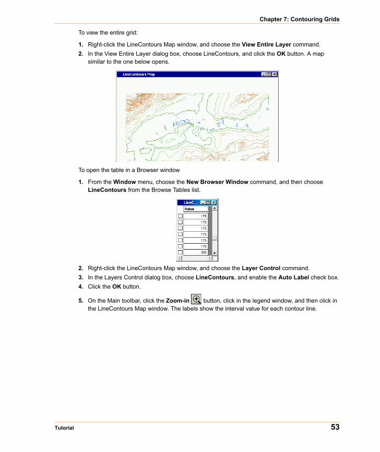
To view the entire grid:
1. Right-click the LineContours Map window, and choose the View Entire Layer command.2. In the View Entire Layer dialog box, choose LineContours, and click the OK button. A map
similar to the one below opens.
To open the table in a Browser window
1. From the Window menu, choose the New Browser Window command, and then choose LineContours from the Browse Tables list.
2. Right-click the LineContours Map window, and choose the Layer Control command.3. In the Layers Control dialog box, choose LineContours, and enable the Auto Label check box.4. Click the OK button.
5. On the Main toolbar, click the Zoom-in button, click in the legend window, and then click in the LineContours Map window. The labels show the interval value for each contour line.
Tutorial 53
Creating Region Contours from a Numeric Grid
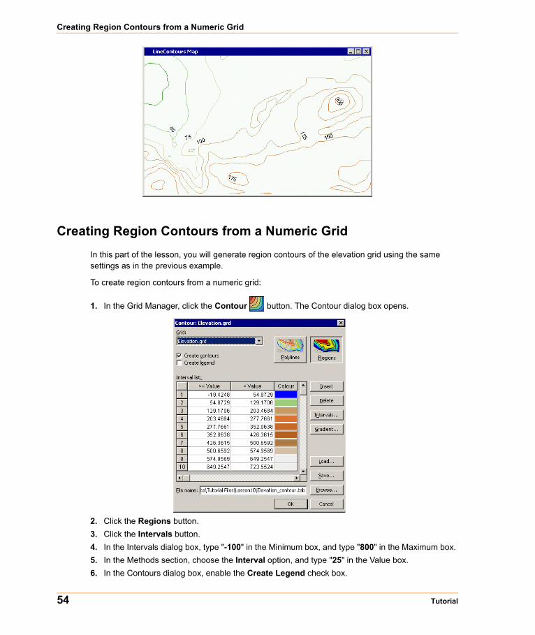
Creating Region Contours from a Numeric GridIn this part of the lesson, you will generate region contours of the elevation grid using the same settings as in the previous example.
To create region contours from a numeric grid:
1. In the Grid Manager, click the Contour button. The Contour dialog box opens.
2. Click the Regions button.3. Click the Intervals button.4. In the Intervals dialog box, type "-100" in the Minimum box, and type "800" in the Maximum box. 5. In the Methods section, choose the Interval option, and type "25" in the Value box.6. In the Contours dialog box, enable the Create Legend check box.
54 Tutorial

Chapter 7: Contouring Grids
7. In the File name box, change the file name to RegionContours.tab, and click the OK button. The colour gradient applied to the contour intervals is by default the same as that of the original grid.
8. Click the Gradient button.9. In the Grid Colour Tool dialog box, change the colour for each interval by double-clicking the
colored box. 10. Click the OK button.11. Click the OK button. Each region has a lower and an upper interval. This is useful for further
analysis, such as selecting all regions within a specified range.
To open the grid in a Browser window:
1. From the Window menu, choose the New Browser Window command. 2. In the Browse Table dialog box, choose RegionContours from the Browse Tables list. The
attribute data assigned to each contour region is displayed in the RegionContours Browser window.
3. From the File menu, choose the Close All command. Ensure that all files are closed before you proceed with the next section.
Contouring a Classified GridYou’ll contour a classified grid using the Contour tool.
To open a table:
1. From the File menu, choose the Open command.2. Choose the LandUse.tab file located in the [User Data]\Tutorial\Lesson07 folder, and click the
Open button.
Tutorial 55

Contouring a Classified Grid
To contour a classified grid:
1. In the Grid Manager, choose the LandUse.tab file, and click the Contour . button.2. In the File name box, change the file name to LandUseContours.tab, and click the Save button.
To view the contoured grid:
1. Right-click the LandUseContours Map window, and choose the View Entire Layer command.2. In the Entire Layer dialog box, choose LandUseContours from the list.3. Click the OK button. The map similar to the one below opens.
4. From the File menu, choose the Close All command. Ensure that all files are closed before you proceed with the next section.
In this lesson, you learned to:
• create a line contour using the Contour tool for a numeric grid• open the legend for a contoured numeric grid• create a region contour using the Contour tool for a numeric grid• view the numeric data assigned to each region• create a region contour using the Contour tool for a classified grid
56 Tutorial

8
Performing Viewshed AnalysisThe Viewshed Analysis tool lets you determine which areas on a grid are visually connected. You’ll use simple viewshed calculations to produce a classified grid that shows the grid cells that are visible and invisible from an observation point. You’ll use complex viewshed calculations to produce a classified grid that shows grid cells that are visible and invisible and shows by how much the object height must be changed for the object to become just visible.
You are a wireless telecommunications operator who has been granted a cellular license in VM City. Your Property Management Division needs to purchase four parcels of land suitable for the location of four towers. Furthermore, the governing municipality has a zoning policy that permits addition of radio masts only upon the submission of both an environmental and a coverage assessment.
Using the Viewshed Analysis function, you will perform two simple viewshed analyses to determine the visible and invisible areas for Tower 1 and for all four towers for a coverage of 15 kilometres in radius.
You also have several remote broadcasting vehicles and need to produce a map showing the vehicle antenna elevation required to receive remote transmissions. You need to determine by how much the heights of these antenna need to be adjusted for them to become visible to each other. You will perform a complex viewshed analysis to obtain this information.
In this lesson, you’ll learn how to
Performing a Simple Viewshed Calculation . . . . . . . . . . . . . . . . .58Performing a Multi-point Viewshed Calculation . . . . . . . . . . . . . .59Performing a Complex Viewshed Calculation . . . . . . . . . . . . . . . .60
Required files can be found in the• [User Data]\Tutorial\Lesson08 folder
Performing a Simple Viewshed Calculation
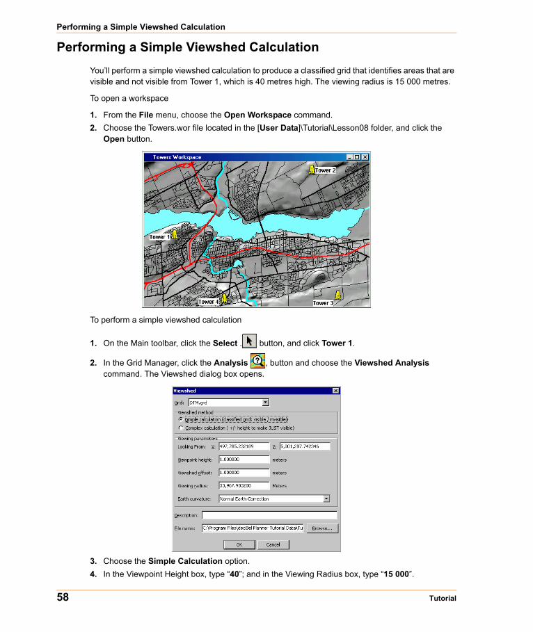
Performing a Simple Viewshed CalculationYou’ll perform a simple viewshed calculation to produce a classified grid that identifies areas that are visible and not visible from Tower 1, which is 40 metres high. The viewing radius is 15 000 metres.
To open a workspace
1. From the File menu, choose the Open Workspace command.2. Choose the Towers.wor file located in the [User Data]\Tutorial\Lesson08 folder, and click the
Open button.
To perform a simple viewshed calculation
1. On the Main toolbar, click the Select . button, and click Tower 1.
2. In the Grid Manager, click the Analysis , button and choose the Viewshed Analysis command. The Viewshed dialog box opens.
3. Choose the Simple Calculation option.4. In the Viewpoint Height box, type “40”; and in the Viewing Radius box, type “15 000”.
58 Tutorial
Chapter 8: Performing Viewshed Analysis
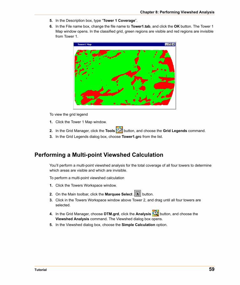
5. In the Description box, type “Tower 1 Coverage”.6. In the File name box, change the file name to Tower1.tab, and click the OK button. The Tower 1
Map window opens. In the classified grid, green regions are visible and red regions are invisible from Tower 1.
To view the grid legend
1. Click the Tower 1 Map window.
2. In the Grid Manager, click the Tools button, and choose the Grid Legends command.3. In the Grid Legends dialog box, choose Tower1.grc from the list.
Performing a Multi-point Viewshed Calculation You’ll perform a multi-point viewshed analysis for the total coverage of all four towers to determine which areas are visible and which are invisible.
To perform a multi-point viewshed calculation
1. Click the Towers Workspace window.
2. On the Main toolbar, click the Marquee Select . button.3. Click in the Towers Workspace window above Tower 2, and drag until all four towers are
selected.
4. In the Grid Manager, choose DTM.grd, click the Analysis button, and choose the Viewshed Analysis command. The Viewshed dialog box opens.
5. In the Viewshed dialog box, choose the Simple Calculation option.
Tutorial 59
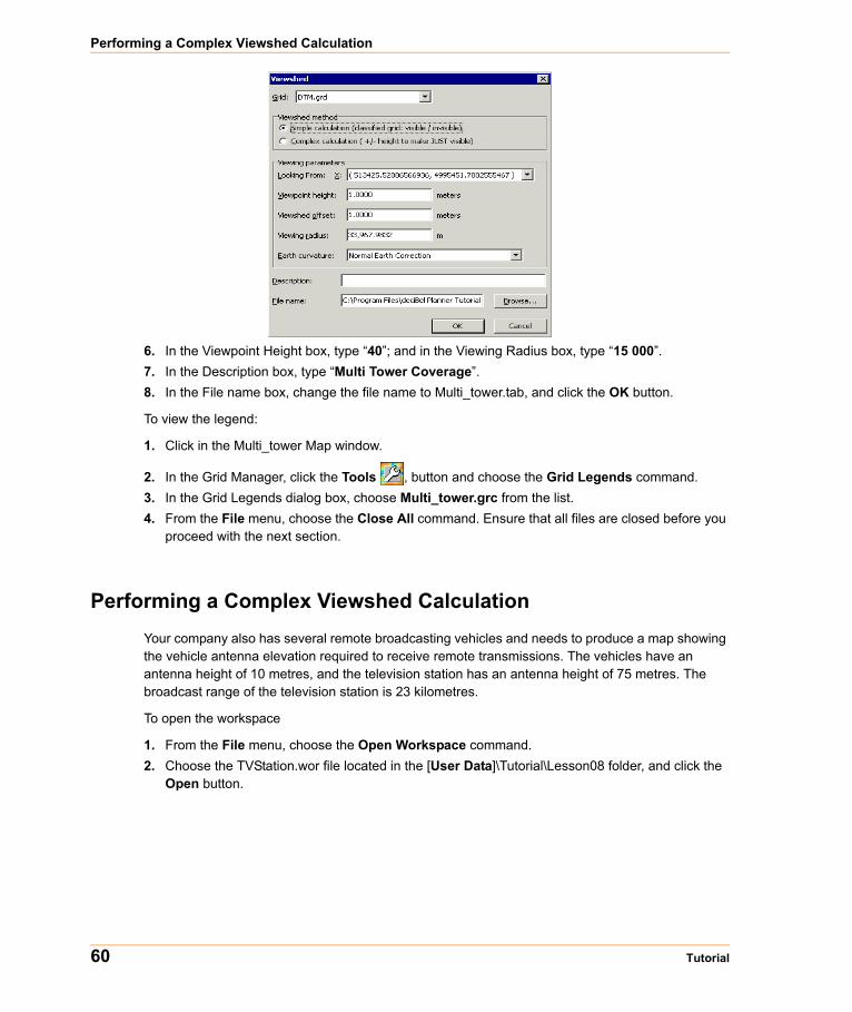
Performing a Complex Viewshed Calculation
6. In the Viewpoint Height box, type “40”; and in the Viewing Radius box, type “15 000”.7. In the Description box, type “Multi Tower Coverage”.8. In the File name box, change the file name to Multi_tower.tab, and click the OK button.
To view the legend:
1. Click in the Multi_tower Map window.
2. In the Grid Manager, click the Tools , button and choose the Grid Legends command.3. In the Grid Legends dialog box, choose Multi_tower.grc from the list.4. From the File menu, choose the Close All command. Ensure that all files are closed before you
proceed with the next section.
Performing a Complex Viewshed CalculationYour company also has several remote broadcasting vehicles and needs to produce a map showing the vehicle antenna elevation required to receive remote transmissions. The vehicles have an antenna height of 10 metres, and the television station has an antenna height of 75 metres. The broadcast range of the television station is 23 kilometres.
To open the workspace
1. From the File menu, choose the Open Workspace command.2. Choose the TVStation.wor file located in the [User Data]\Tutorial\Lesson08 folder, and click the
Open button.
60 Tutorial
Chapter 8: Performing Viewshed Analysis
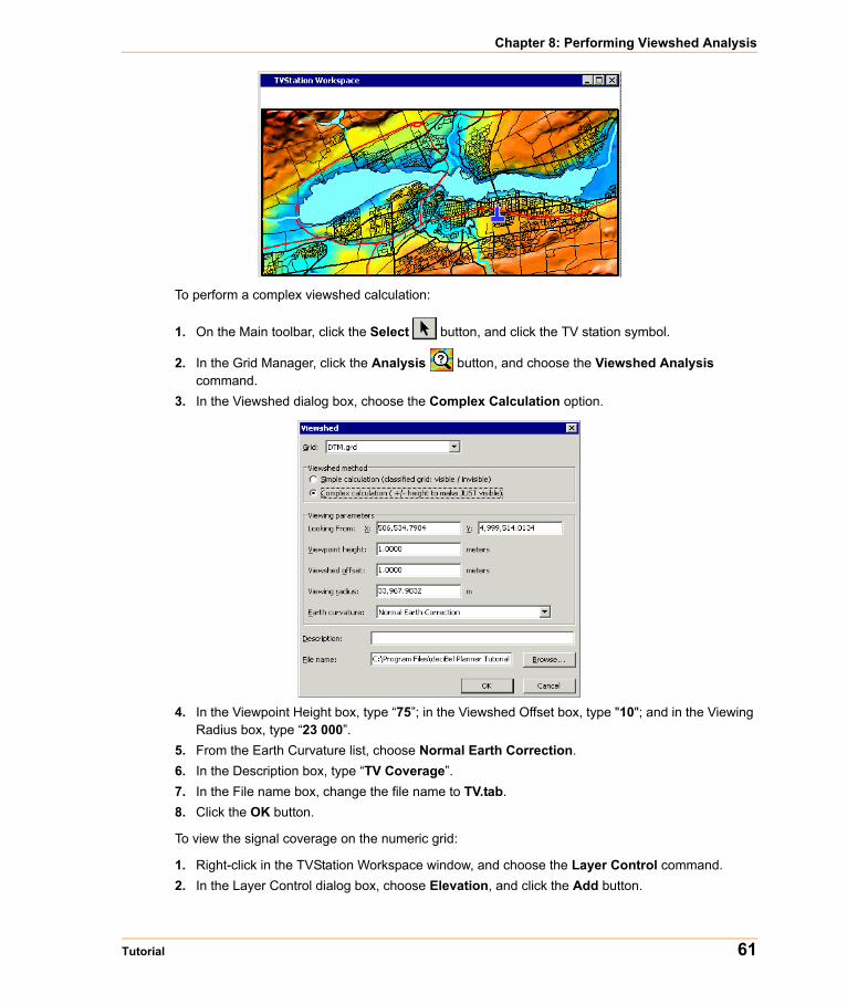
To perform a complex viewshed calculation:
1. On the Main toolbar, click the Select button, and click the TV station symbol.
2. In the Grid Manager, click the Analysis button, and choose the Viewshed Analysis command.
3. In the Viewshed dialog box, choose the Complex Calculation option.
4. In the Viewpoint Height box, type “75”; in the Viewshed Offset box, type "10"; and in the Viewing Radius box, type “23 000”.
5. From the Earth Curvature list, choose Normal Earth Correction.6. In the Description box, type “TV Coverage”.7. In the File name box, change the file name to TV.tab.8. Click the OK button.
To view the signal coverage on the numeric grid:
1. Right-click in the TVStation Workspace window, and choose the Layer Control command.2. In the Layer Control dialog box, choose Elevation, and click the Add button.
Tutorial 61
Performing a Complex Viewshed Calculation
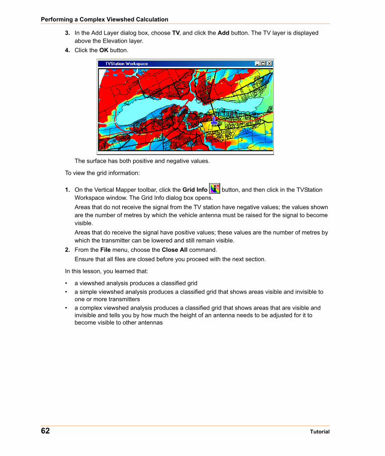
3. In the Add Layer dialog box, choose TV, and click the Add button. The TV layer is displayed above the Elevation layer.
4. Click the OK button.
The surface has both positive and negative values.
To view the grid information:
1. On the Vertical Mapper toolbar, click the Grid Info button, and then click in the TVStation Workspace window. The Grid Info dialog box opens.Areas that do not receive the signal from the TV station have negative values; the values shown are the number of metres by which the vehicle antenna must be raised for the signal to become visible. Areas that do receive the signal have positive values; these values are the number of metres by which the transmitter can be lowered and still remain visible.
2. From the File menu, choose the Close All command.Ensure that all files are closed before you proceed with the next section.
In this lesson, you learned that:
• a viewshed analysis produces a classified grid• a simple viewshed analysis produces a classified grid that shows areas visible and invisible to
one or more transmitters• a complex viewshed analysis produces a classified grid that shows areas that are visible and
invisible and tells you by how much the height of an antenna needs to be adjusted for it to become visible to other antennas
62 Tutorial
9
Determining Point-to-Point IntervisibilityIntervisibility is the ability to see in a direct line of sight from one position on the earth’s surface to another. The Point-to-Point Intervisibility function analyzes the terrain between two given points and tells you whether or not the two points are intervisible. It also tells you where along the line a point at a specified height above the ground is visible.
You are a telecommunications operator who needs to install two microwave relay towers. You’ll need to find two locations with unimpeded visibility for these towers.You’ll test two potential locations for each tower for intervisibility.
In this lesson, you’ll learn:
Determining Intervisibility using an Existing Line . . . . . . . . . . . .64Determining the Intervisibility Height. . . . . . . . . . . . . . . . . . . . . . .66Using a Virtual Line to Determine Intervisibility . . . . . . . . . . . . . .66
Required files can be found in:• [User Data]\Tutorial\Lesson09
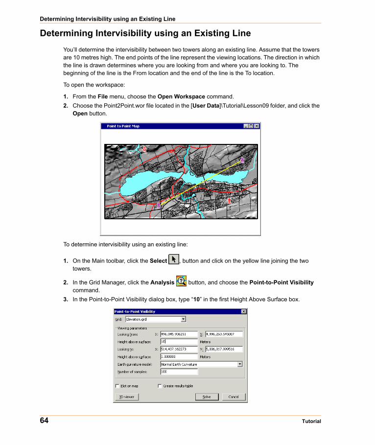
Determining Intervisibility using an Existing Line
Determining Intervisibility using an Existing LineYou’ll determine the intervisibility between two towers along an existing line. Assume that the towers are 10 metres high. The end points of the line represent the viewing locations. The direction in which the line is drawn determines where you are looking from and where you are looking to. The beginning of the line is the From location and the end of the line is the To location.
To open the workspace:
1. From the File menu, choose the Open Workspace command.2. Choose the Point2Point.wor file located in the [User Data]\Tutorial\Lesson09 folder, and click the
Open button.
To determine intervisibility using an existing line:
1. On the Main toolbar, click the Select , button and click on the yellow line joining the two towers.
2. In the Grid Manager, click the Analysis button, and choose the Point-to-Point Visibility command.
3. In the Point-to-Point Visibility dialog box, type “10” in the first Height Above Surface box.
64 Tutorial
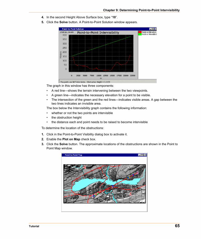
Chapter 9: Determining Point-to-Point Intervisibility
4. In the second Height Above Surface box, type “10”. 5. Click the Solve button. A Point-to-Point Solution window appears.
The graph in this window has three components:• A red line—shows the terrain intervening between the two viewpoints. • A green line—indicates the necessary elevation for a point to be visible. • The intersection of the green and the red lines—indicates visible areas. A gap between the
two lines indicates an invisible area.The box below the Intervisibility graph contains the following information:• whether or not the two points are intervisible• the obstruction height• the distance each end point needs to be raised to become intervisible
To determine the location of the obstructions:
1. Click in the Point-to-Point Visibility dialog box to activate it.2. Enable the Plot on Map check box. 3. Click the Solve button. The approximate locations of the obstructions are shown in the Point to
Point Map window.
Tutorial 65
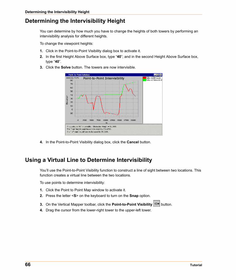
Determining the Intervisibility Height
Determining the Intervisibility HeightYou can determine by how much you have to change the heights of both towers by performing an intervisibility analysis for different heights.
To change the viewpoint heights:
1. Click in the Point-to-Point Visibility dialog box to activate it.2. In the first Height Above Surface box, type “40”; and in the second Height Above Surface box,
type “40”.3. Click the Solve button. The towers are now intervisible.
4. In the Point-to-Point Visibility dialog box, click the Cancel button.
Using a Virtual Line to Determine IntervisibilityYou’ll use the Point-to-Point Visibility function to construct a line of sight between two locations. This function creates a virtual line between the two locations.
To use points to determine intervisibility:
1. Click the Point to Point Map window to activate it.2. Press the letter <S> on the keyboard to turn on the Snap option.
3. On the Vertical Mapper toolbar, click the Point-to-Point Visibility button.4. Drag the cursor from the lower-right tower to the upper-left tower.
66 Tutorial

Chapter 9: Determining Point-to-Point Intervisibility
5. In the Point to Point Visibility dialog box, enable the Create Results Table check box.6. In the first Height Above Surface box, type “1.5”, and in the second Height Above Surface box,
type “1.5”.7. Click the Solve button. The towers are not intervisible.
A Browser window opens, showing the distance to viewable elevation, to surface elevation, and to relative elevations.
8. From the File menu, choose the Close All command. Ensure that all files are closed before you proceed with the next section.
In this lesson, you learned to:
• use the Point-to-Point intervisibility command to generate a graph that shows where two locations are and are not intervisible
• determine intervisibility using a line on the grid and using two points• view the location of the obstructions in the Map window• determine the height for intervisibility by changing the Height above surface values in the Point-
to-Point Intervisibility dialog box• generate a results table showing the distance to viewable elevation, to surface elevation, and to
relative elevations
Tutorial 67

Using a Virtual Line to Determine Intervisibility
68 Tutorial
10
Modifying Grids Using the Grid CalculatorThe Grid Calculator is designed to look and to operate like a scientific calculator, applying mathematical expressions to one or more grids. Calculations are performed on a cell-by-cell basis for each grid entered into the expression. Generally, this tool is used to prepare data for further analysis.
In this lesson, you’ll learn:
Creating a Grid Math Expression . . . . . . . . . . . . . . . . . . . . . . . . . .70Normalizing Grid Values . . . . . . . . . . . . . . . . . . . . . . . . . . . . . . . . .71Using a Saved Expression to Normalize Grid Values . . . . . . . . . .72
Required files can be found in:
• [User Data]\Tutorial\Lesson10 folder
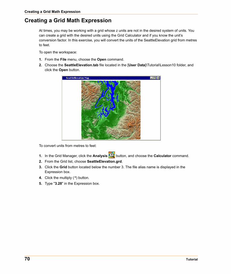
Creating a Grid Math Expression
Creating a Grid Math ExpressionAt times, you may be working with a grid whose z units are not in the desired system of units. You can create a grid with the desired units using the Grid Calculator and if you know the unit’s conversion factor. In this exercise, you will convert the units of the SeattleElevation grid from metres to feet.
To open the workspace:
1. From the File menu, choose the Open command.2. Choose the SeattleElevation.tab file located in the [User Data]\Tutorial\Lesson10 folder, and
click the Open button.
To convert units from metres to feet:
1. In the Grid Manager, click the Analysis button, and choose the Calculator command. 2. From the Grid list, choose SeattleElevation.grd.3. Click the Grid button located below the number 3. The file alias name is displayed in the
Expression box.4. Click the multiply (*) button.5. Type "3.28" in the Expression box.
70 Tutorial

Chapter 10: Modifying Grids Using the Grid Calculator
6. Click the OK button.7. In the Grid Calculator - Save dialog box, change the file name to SeattleElevation_Ft.tab in the
Save the New Grid as box.8. From the Z-unit Type list, choose Feet, and click the OK button. The SeattleElevation_Ft Map
window opens.
9. On the Vertical Mapper toolbar, click the Grid Info button.10. Click the SeattleElevation_Ft Map window. The Grid Info dialog box opens. The values in the
SeattleElevation_Ft.grd grid are 3.28 times larger than those in the SeattleElevation.grd grid.
Normalizing Grid Values When a data set is normalized, the range of values in that data set are spread over a range between zero and one. Two or more normalized data sets, which may have different units of measure or which are in different geographic locations, can thus be compared.
The basic formula for normalizing a data set is
(GRID - GRIDmin)/(GRIDmax - GRIDmin)
In this exercise, you will normalize the z-values in the SeattleElevation.grd file to between zero and one. When normalizing values, you can use the range shown in the grid or any range you choose. In this example, you will normalize the z -value between the minimum and the maximum.
To normalize grid values:
1. In the Grid Manager, choose SeattleElevation.grd, and click the Info button.2. Click the Z-units tab, and write down the value shown in the Z-max field. The Z-max value is
4373.93. The Z-min value is assumed to be zero.
3. In the Grid Manager, click the Analysis button, and choose the Calculator command.4. In the Calculator dialog box, click the brackets ( ) button.
Tutorial 71

Using a Saved Expression to Normalize Grid Values
5. From the Grids list, choose SeattleElevation.grd, and click the Grid button.6. Type "-0)/(4373.93-0)" in the Expression box.7. Click the Save As button, type "Normalized.exp" in the File Name box, and click the Save
button. You have saved the expression in a *.exp file.8. In the Calculator dialog box, click the OK button.9. In the Grid Calculator - Save dialog box, change the file name to SeattleElevNorm.tab.10. In the Enter User Defined Type box, type "Normalized to 1".
11. Click the OK button. The SeattleElevNorm Map window opens.
To inspect the normalized grid:
1. On the Vertical Mapper toolbar, click the Grid Info . button.2. Click in the SeattleElevNorm Map window. The values shown in the Grid Info dialog box are
normalized between zero and one.
Using a Saved Expression to Normalize Grid Values You can apply the same normalization formula to other grids. This saves you time, because you don't need to type the expression again.
In this part of the lesson, you will normalize the SeattleElevation grid using the expression you saved in the previous exercise.
To open the file:
• In the Grid Manager, click the Open Grid button, and choose the SeattleElevation_trim.tab file located in the C:\Program Files\MapInfo\Professional\vm\Tutorial\Lesson10 folder, and click the OK button.
To use a saved expression to normalize grid values:
1. In the Grid Manager, click the Analysis , button and choose the Calculator command.2. In the Grids list, choose SeattleElevation.grd, and click the Delete button.3. Click the Load button.4. In the Load Expression dialog box, choose Normalized.exp, and click the Open button. 5. In the Grid Math Expression Viewer dialog box, enable the Use as a Complete Expression
option.6. Choose the expression, click the Insert button, and click the Close button.
72 Tutorial

Chapter 10: Modifying Grids Using the Grid Calculator
7. From the Grids list, choose SeattleElevation_trim.grd, and click the Modify button.8. In the Variable Editor dialog box, type "Grid1" in the Alias box, and click the OK button.
The alias for SeattleElevation_trim.grd now corresponds to that shown in the equation.9. Click the OK button. 10. In the Grid Calculator - Save dialog box, change the file name to Seattle2.tab in the File Name
box.11. In the User Defined Type box, type "Normalized to 1", and click the OK button. The Seattle2
Map window opens.
To view the information on the Z-tab:
1. In the Grid Manager, choose Seattle2.grd. The information shown on the Z-tab is for Seattle2.grd.
2. From the File menu, choose the Close All command. Ensure that all files are closed before you proceed with the next section.
In this lesson, you learned that you can:
• Multiply numbers in a grid using the Calculator• Add And subtract numbers in grids• Save mathematical expressions and apply them to other grids
Tutorial 73

Using a Saved Expression to Normalize Grid Values
74 Tutorial

11
Performing a Grid QueryYou are an RF operator who needs to identify areas in the Seattle area that are at or below an elevation of 100 m above sea level, the Urban/Residential areas in the Seattle area that have Transmitter Signal Strength values equal to or less than -75 dB, and the Urban/Residential and Urban/Industrial areas in the Seattle area that have Transmitter Signal Strength values equal to or greater than -75 dB.
In this lesson, you’ll learn:
Creating a Simple Query . . . . . . . . . . . . . . . . . . . . . . . . . . . . . . . . .76Performing a Query using Two Grids. . . . . . . . . . . . . . . . . . . . . . .78Performing a Query using Two Grids and Multiple Conditions . .80
Required files:
• [User Data]\Tutorial\Lesson11
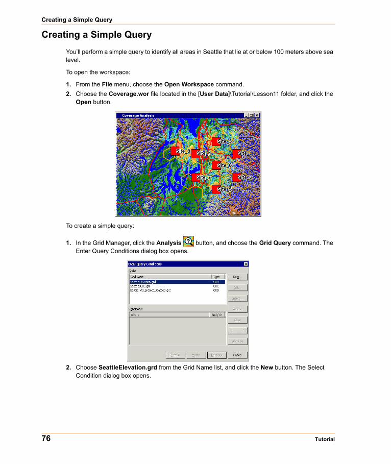
Creating a Simple Query
Creating a Simple QueryYou’ll perform a simple query to identify all areas in Seattle that lie at or below 100 meters above sea level.
To open the workspace:
1. From the File menu, choose the Open Workspace command.2. Choose the Coverage.wor file located in the [User Data]\Tutorial\Lesson11 folder, and click the
Open button.
To create a simple query:
1. In the Grid Manager, click the Analysis button, and choose the Grid Query command. The Enter Query Conditions dialog box opens.
2. Choose SeattleElevation.grd from the Grid Name list, and click the New button. The Select Condition dialog box opens.
76 Tutorial
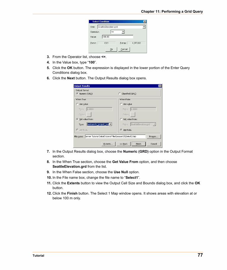
Chapter 11: Performing a Grid Query
3. From the Operator list, choose <=.4. In the Value box, type “100”.5. Click the OK button. The expression is displayed in the lower portion of the Enter Query
Conditions dialog box.6. Click the Next button. The Output Results dialog box opens.
7. In the Output Results dialog box, choose the Numeric (GRD) option in the Output Format section.
8. In the When True section, choose the Get Value From option, and then choose SeattleElevation.grd from the list.
9. In the When False section, choose the Use Null option.10. In the File name box, change the file name to “Select1”.11. Click the Extents button to view the Output Cell Size and Bounds dialog box, and click the OK
button.12. Click the Finish button. The Select 1 Map window opens. It shows areas with elevation at or
below 100 m only.
Tutorial 77
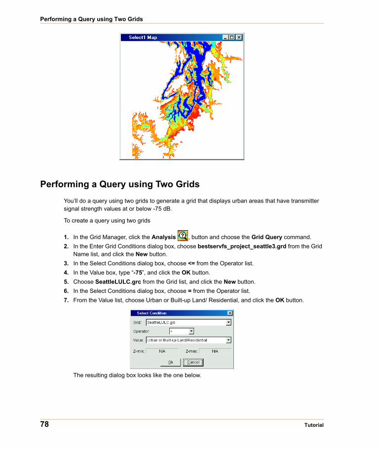
Performing a Query using Two Grids
Performing a Query using Two GridsYou’ll do a query using two grids to generate a grid that displays urban areas that have transmitter signal strength values at or below -75 dB.
To create a query using two grids
1. In the Grid Manager, click the Analysis , button and choose the Grid Query command.2. In the Enter Grid Conditions dialog box, choose bestservfs_project_seattle3.grd from the Grid
Name list, and click the New button.3. In the Select Conditions dialog box, choose <= from the Operator list.4. In the Value box, type “-75”, and click the OK button.5. Choose SeattleLULC.grc from the Grid list, and click the New button.6. In the Select Conditions dialog box, choose = from the Operator list.7. From the Value list, choose Urban or Built-up Land/ Residential, and click the OK button.
The resulting dialog box looks like the one below.
78 Tutorial
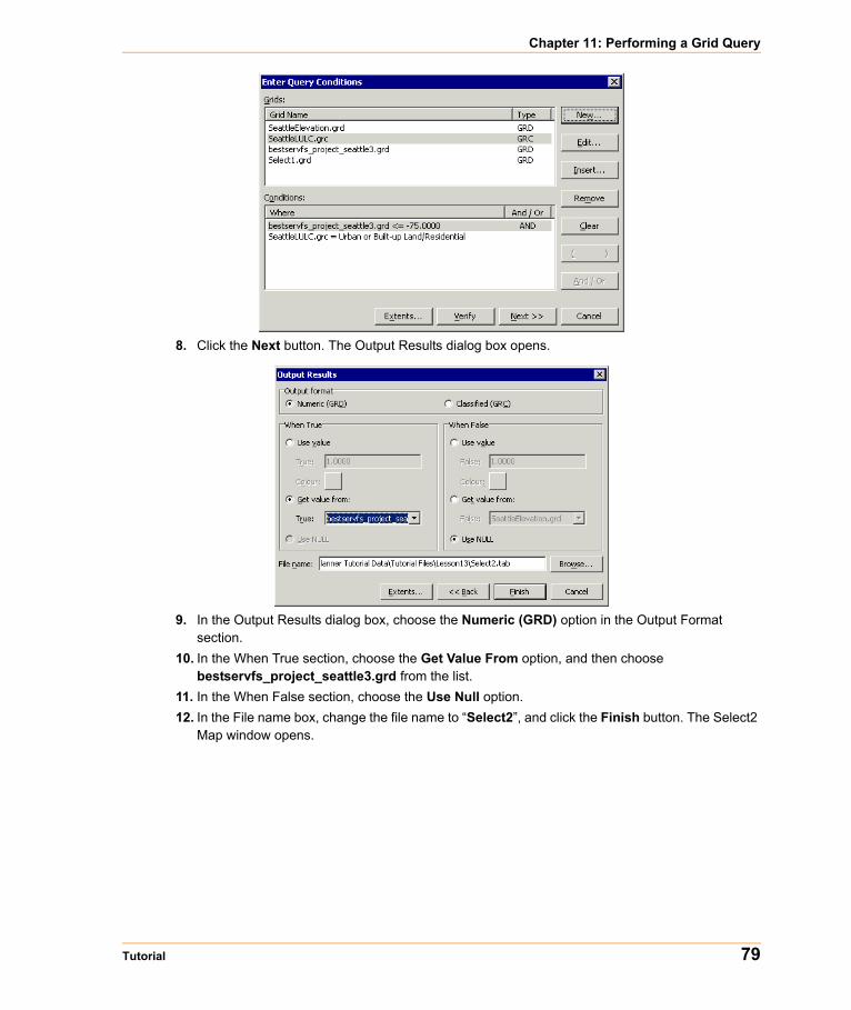
Chapter 11: Performing a Grid Query
8. Click the Next button. The Output Results dialog box opens.
9. In the Output Results dialog box, choose the Numeric (GRD) option in the Output Format section.
10. In the When True section, choose the Get Value From option, and then choose bestservfs_project_seattle3.grd from the list.
11. In the When False section, choose the Use Null option.12. In the File name box, change the file name to “Select2”, and click the Finish button. The Select2
Map window opens.
Tutorial 79
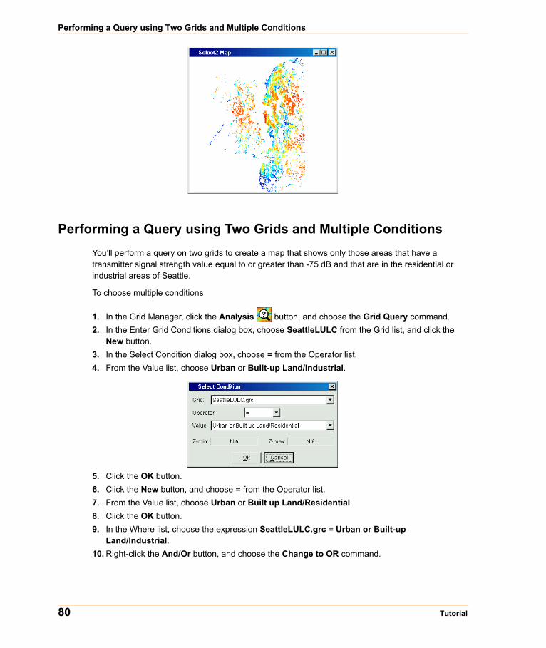
Performing a Query using Two Grids and Multiple Conditions
Performing a Query using Two Grids and Multiple ConditionsYou’ll perform a query on two grids to create a map that shows only those areas that have a transmitter signal strength value equal to or greater than -75 dB and that are in the residential or industrial areas of Seattle.
To choose multiple conditions
1. In the Grid Manager, click the Analysis button, and choose the Grid Query command.2. In the Enter Grid Conditions dialog box, choose SeattleLULC from the Grid list, and click the
New button.3. In the Select Condition dialog box, choose = from the Operator list.4. From the Value list, choose Urban or Built-up Land/Industrial.
5. Click the OK button.6. Click the New button, and choose = from the Operator list.7. From the Value list, choose Urban or Built up Land/Residential.8. Click the OK button.9. In the Where list, choose the expression SeattleLULC.grc = Urban or Built-up
Land/Industrial.10. Right-click the And/Or button, and choose the Change to OR command.
80 Tutorial
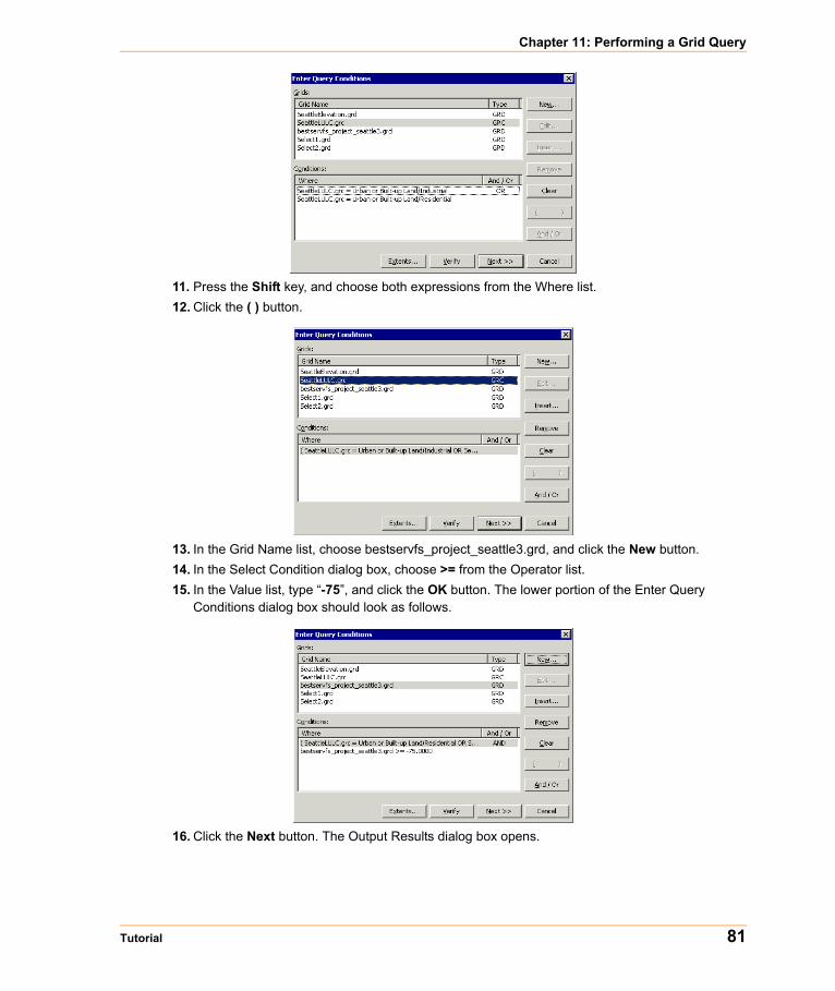
Chapter 11: Performing a Grid Query
11. Press the Shift key, and choose both expressions from the Where list.12. Click the ( ) button.
13. In the Grid Name list, choose bestservfs_project_seattle3.grd, and click the New button.14. In the Select Condition dialog box, choose >= from the Operator list.15. In the Value list, type “-75”, and click the OK button. The lower portion of the Enter Query
Conditions dialog box should look as follows.
16. Click the Next button. The Output Results dialog box opens.
Tutorial 81
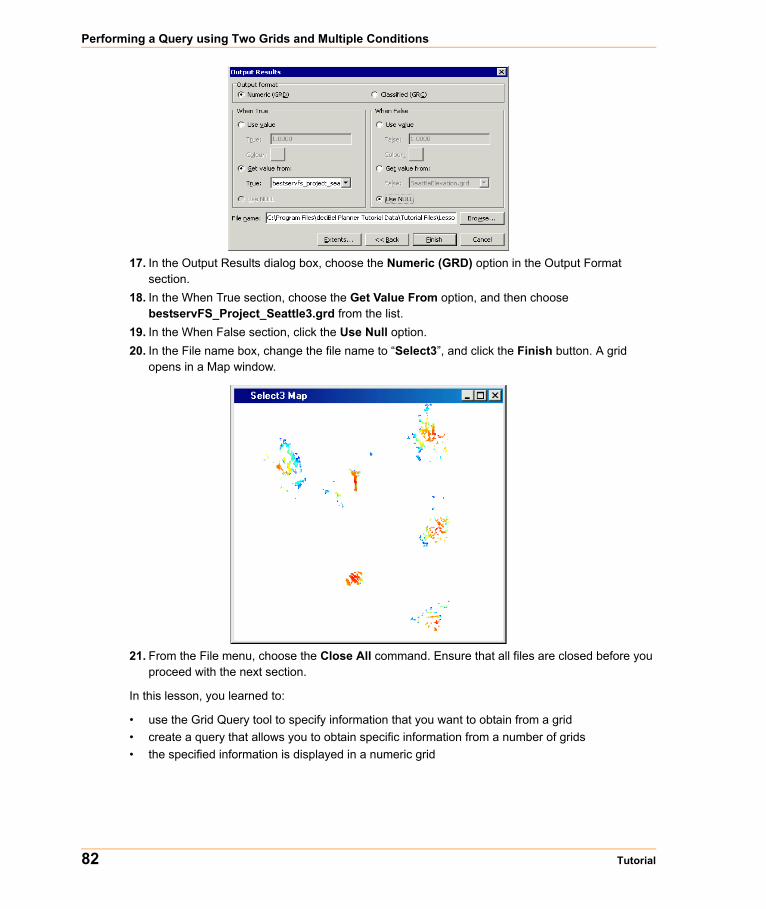
Performing a Query using Two Grids and Multiple Conditions
17. In the Output Results dialog box, choose the Numeric (GRD) option in the Output Format section.
18. In the When True section, choose the Get Value From option, and then choose bestservFS_Project_Seattle3.grd from the list.
19. In the When False section, click the Use Null option.20. In the File name box, change the file name to “Select3”, and click the Finish button. A grid
opens in a Map window.
21. From the File menu, choose the Close All command. Ensure that all files are closed before you proceed with the next section.
In this lesson, you learned to:
• use the Grid Query tool to specify information that you want to obtain from a grid• create a query that allows you to obtain specific information from a number of grids• the specified information is displayed in a numeric grid
82 Tutorial

12
Obtaining Statistical DataIn many applications, there is often a need to attribute vector objects with information obtained from gridded information.
As it applies to grid geometry, slope is a measurement of the "steepness" of a grid cell in three-dimensional space and is, therefore, most applicable to elevation surfaces. In Vertical Mapper, slope is calculated by averaging the slopes of the eight triangle faces that are formed from the surrounding nodes.
In this lesson, you’ll learn:
Comparing Predicted to Measured Transmitter Signal Strength, p. 84Creating a Slope Grid, p. 85Obtaining Statistics using the Line Info and the Line Inspection Tools, p. 86Obtaining Statistics using the Region Info and the Region Inspection Tools, p. 88
Required files can be found in:
• [User Data]\Tutorial\Lesson12 folder
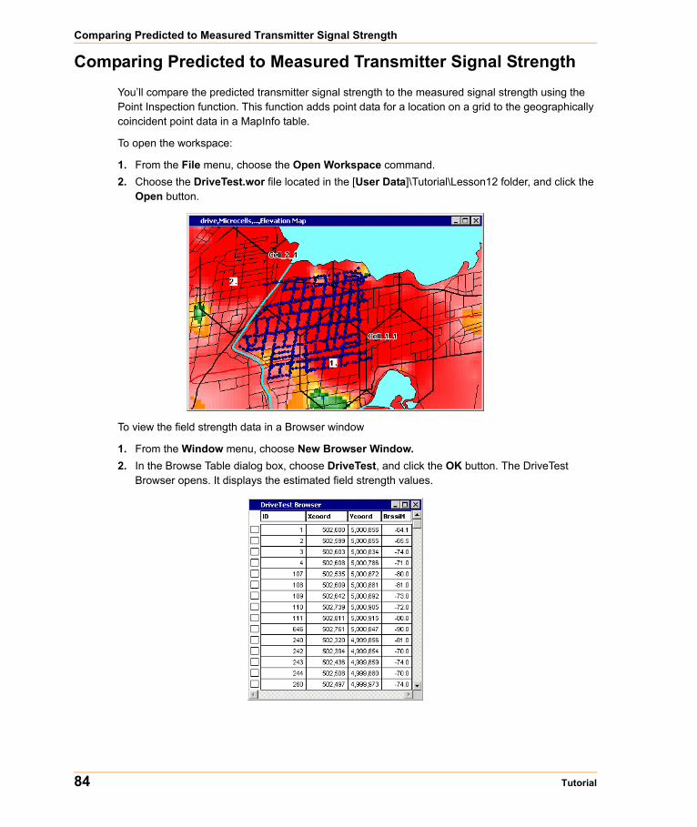
Comparing Predicted to Measured Transmitter Signal Strength
Comparing Predicted to Measured Transmitter Signal StrengthYou’ll compare the predicted transmitter signal strength to the measured signal strength using the Point Inspection function. This function adds point data for a location on a grid to the geographically coincident point data in a MapInfo table.
To open the workspace:
1. From the File menu, choose the Open Workspace command.2. Choose the DriveTest.wor file located in the [User Data]\Tutorial\Lesson12 folder, and click the
Open button.
To view the field strength data in a Browser window
1. From the Window menu, choose New Browser Window.2. In the Browse Table dialog box, choose DriveTest, and click the OK button. The DriveTest
Browser opens. It displays the estimated field strength values.
84 Tutorial
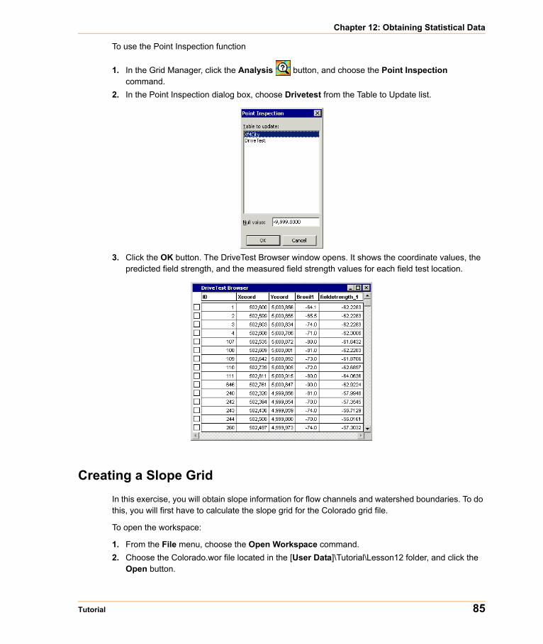
Chapter 12: Obtaining Statistical Data
To use the Point Inspection function
1. In the Grid Manager, click the Analysis button, and choose the Point Inspection command.
2. In the Point Inspection dialog box, choose Drivetest from the Table to Update list.
3. Click the OK button. The DriveTest Browser window opens. It shows the coordinate values, the predicted field strength, and the measured field strength values for each field test location.
Creating a Slope GridIn this exercise, you will obtain slope information for flow channels and watershed boundaries. To do this, you will first have to calculate the slope grid for the Colorado grid file.
To open the workspace:
1. From the File menu, choose the Open Workspace command.2. Choose the Colorado.wor file located in the [User Data]\Tutorial\Lesson12 folder, and click the
Open button.
Tutorial 85
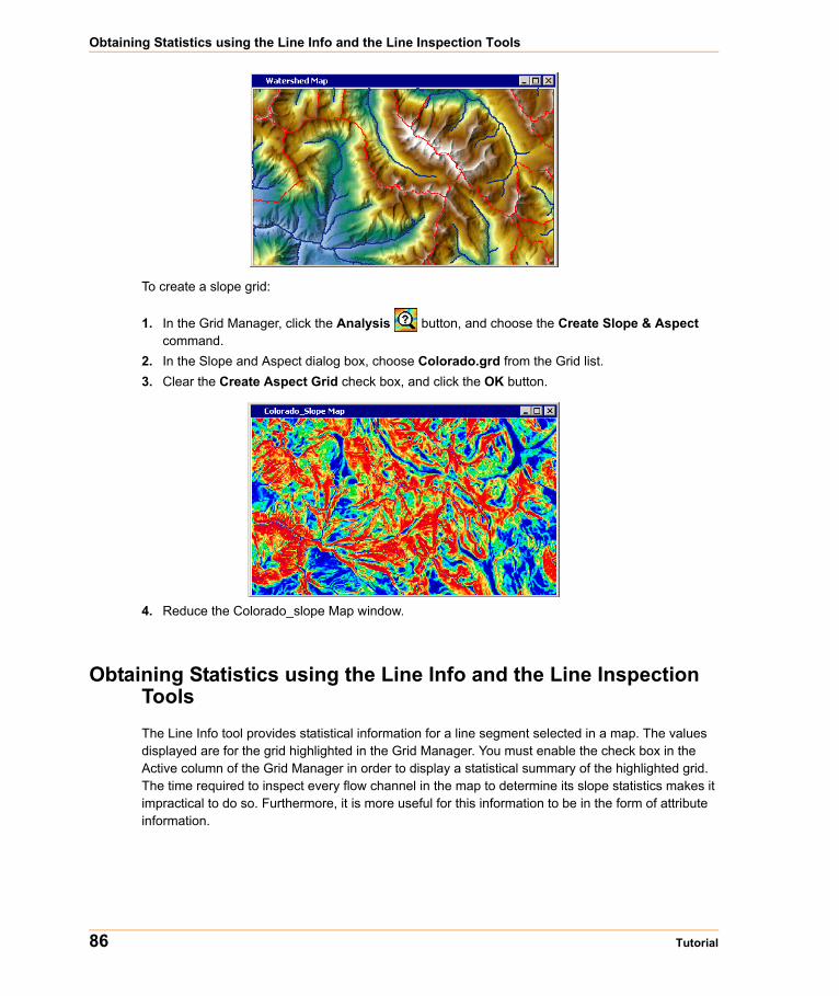
Obtaining Statistics using the Line Info and the Line Inspection Tools
To create a slope grid:
1. In the Grid Manager, click the Analysis button, and choose the Create Slope & Aspect command.
2. In the Slope and Aspect dialog box, choose Colorado.grd from the Grid list.3. Clear the Create Aspect Grid check box, and click the OK button.
4. Reduce the Colorado_slope Map window.
Obtaining Statistics using the Line Info and the Line Inspection ToolsThe Line Info tool provides statistical information for a line segment selected in a map. The values displayed are for the grid highlighted in the Grid Manager. You must enable the check box in the Active column of the Grid Manager in order to display a statistical summary of the highlighted grid. The time required to inspect every flow channel in the map to determine its slope statistics makes it impractical to do so. Furthermore, it is more useful for this information to be in the form of attribute information.
86 Tutorial
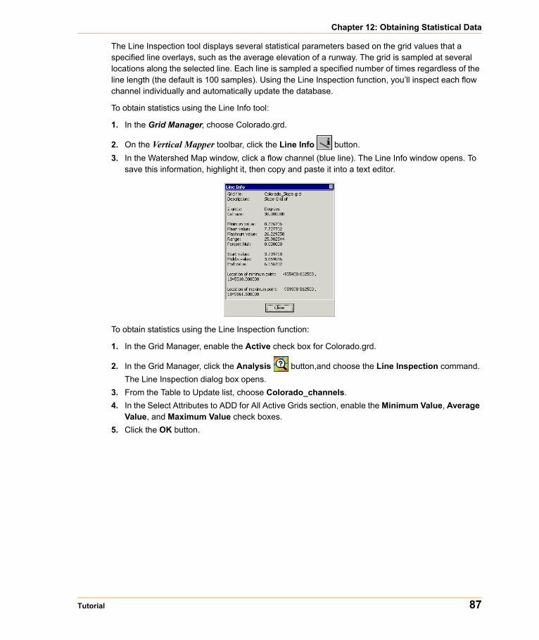
Chapter 12: Obtaining Statistical Data
The Line Inspection tool displays several statistical parameters based on the grid values that a specified line overlays, such as the average elevation of a runway. The grid is sampled at several locations along the selected line. Each line is sampled a specified number of times regardless of the line length (the default is 100 samples). Using the Line Inspection function, you’ll inspect each flow channel individually and automatically update the database.
To obtain statistics using the Line Info tool:
1. In the Grid Manager, choose Colorado.grd.
2. On the Vertical Mapper toolbar, click the Line Info button.3. In the Watershed Map window, click a flow channel (blue line). The Line Info window opens. To
save this information, highlight it, then copy and paste it into a text editor.
To obtain statistics using the Line Inspection function:
1. In the Grid Manager, enable the Active check box for Colorado.grd.
2. In the Grid Manager, click the Analysis button,and choose the Line Inspection command.The Line Inspection dialog box opens.
3. From the Table to Update list, choose Colorado_channels.4. In the Select Attributes to ADD for All Active Grids section, enable the Minimum Value, Average
Value, and Maximum Value check boxes.5. Click the OK button.
Tutorial 87

Obtaining Statistics using the Region Info and the Region Inspection Tools
Obtaining Statistics using the Region Info and the Region Inspection ToolsThe Region Info tool displays a statistical summary of the data within a selected region. The values displayed are for the grid highlighted in the Grid Manager. You must enable the check box in the Active column of the Grid Manager in order to display a statistical summary of the highlighted grid.
The Region Inspection function updates a MapInfo table of regions with new columns of values taken from one or more geographically coincident grid files. The process inspects the grid file underlying each region, returns a selected number of statistical parameters calculated from the range of grid values lying within each region, and writes the value to a new column in the region table.
To obtain information using the Region Info tool:
1. On the Vertical Mapper toolbar, click the Region Info button. 2. Click a watershed boundary in the Watershed Map window. The Region Info window opens.
To obtain information using the Region Inspection function
1. In the Grid Manager, enable the Active check box for Colorado.grd.
2. In the Grid Manager, click the Analysis , button and choose the Region Inspection command.
3. In the Region Inspection dialog box, choose Colorado_channels.4. Enable the Minimum Value, Average Value, and Maximum Value check boxes in the Select
Attribute Information to Add for All Active Grids section.5. Click the OK button.
88 Tutorial
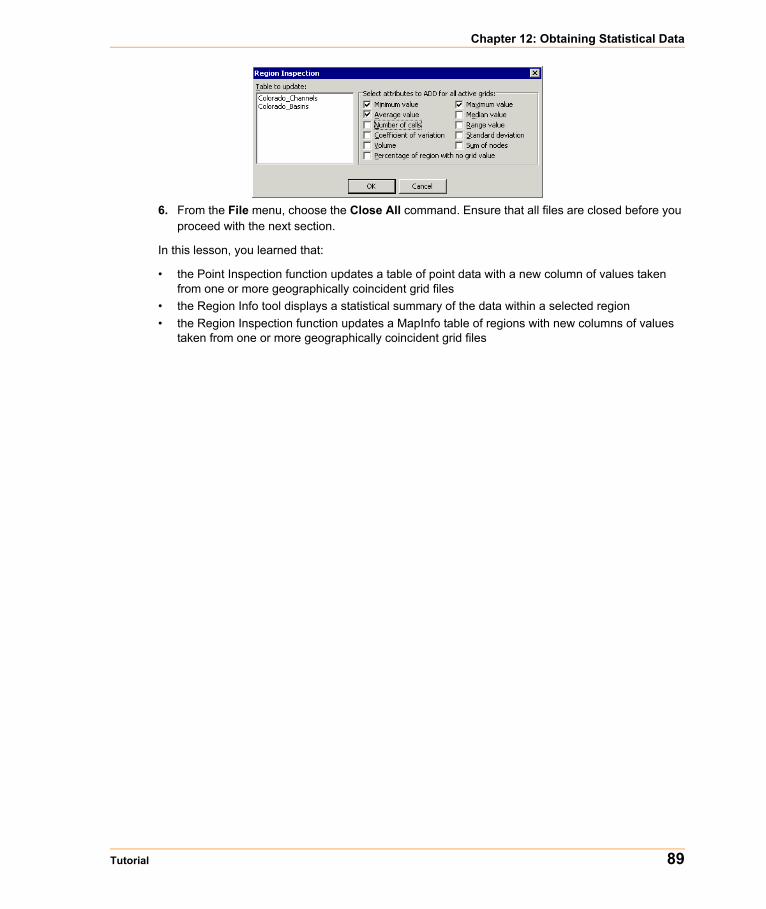
Chapter 12: Obtaining Statistical Data
6. From the File menu, choose the Close All command. Ensure that all files are closed before you proceed with the next section.
In this lesson, you learned that:
• the Point Inspection function updates a table of point data with a new column of values taken from one or more geographically coincident grid files
• the Region Info tool displays a statistical summary of the data within a selected region • the Region Inspection function updates a MapInfo table of regions with new columns of values
taken from one or more geographically coincident grid files
Tutorial 89

Obtaining Statistics using the Region Info and the Region Inspection Tools
90 Tutorial

13
Using the Correlation ToolCorrelation analysis investigates relationships between numerical grids. A correlation matrix lets you examine the correlation between a group of numeric grids. All permutations of pairs of grids in the selection are analyzed, and the results are returned in a matrix.
The Predictive Analysis tool enables you to identify areas in multiple grids with similar characteristics based the statistical characteristics. This is a useful tool for site selection problems such as locating retail stores where you have a known successful location and you wish to determine other possible successful locations.
In this lesson, you’ll learn:
Performing a Correlation Analysis . . . . . . . . . . . . . . . . . . . . . . . . .92Grouping Correlation Data . . . . . . . . . . . . . . . . . . . . . . . . . . . . . . .94Performing a Predictive Analysis . . . . . . . . . . . . . . . . . . . . . . . . . .96
Required files can be found in:• [User Data]\Tutorial\Lesson13
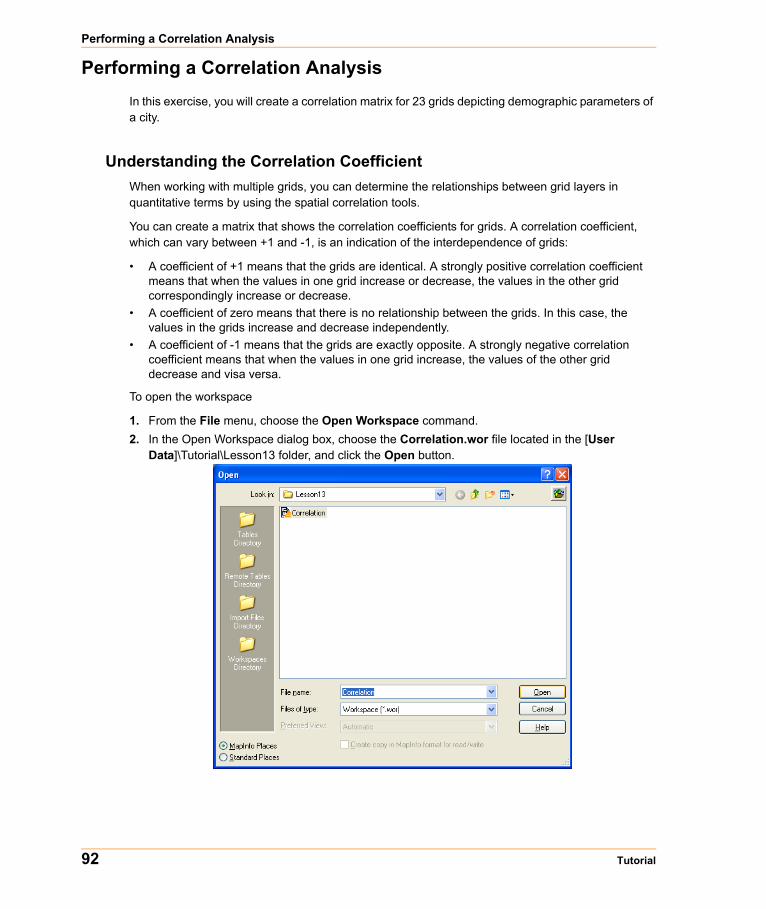
Performing a Correlation Analysis
Performing a Correlation AnalysisIn this exercise, you will create a correlation matrix for 23 grids depicting demographic parameters of a city.
Understanding the Correlation CoefficientWhen working with multiple grids, you can determine the relationships between grid layers in quantitative terms by using the spatial correlation tools.
You can create a matrix that shows the correlation coefficients for grids. A correlation coefficient, which can vary between +1 and -1, is an indication of the interdependence of grids:
• A coefficient of +1 means that the grids are identical. A strongly positive correlation coefficient means that when the values in one grid increase or decrease, the values in the other grid correspondingly increase or decrease.
• A coefficient of zero means that there is no relationship between the grids. In this case, the values in the grids increase and decrease independently.
• A coefficient of -1 means that the grids are exactly opposite. A strongly negative correlation coefficient means that when the values in one grid increase, the values of the other grid decrease and visa versa.
To open the workspace
1. From the File menu, choose the Open Workspace command.2. In the Open Workspace dialog box, choose the Correlation.wor file located in the [User
Data]\Tutorial\Lesson13 folder, and click the Open button.
92 Tutorial
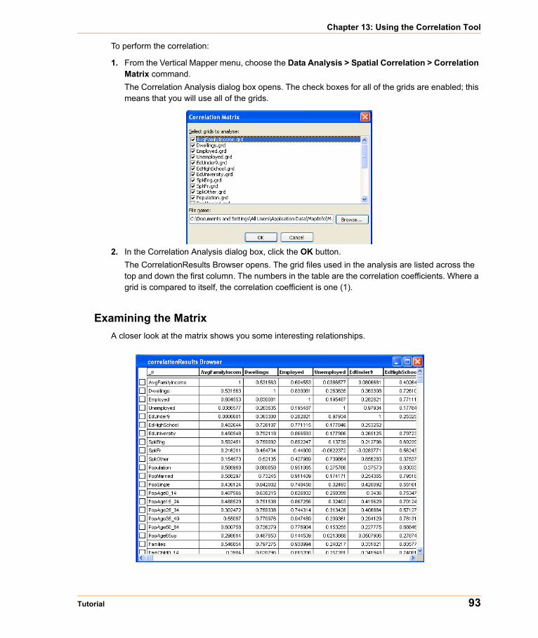
Chapter 13: Using the Correlation Tool
To perform the correlation:
1. From the Vertical Mapper menu, choose the Data Analysis > Spatial Correlation > Correlation Matrix command.The Correlation Analysis dialog box opens. The check boxes for all of the grids are enabled; this means that you will use all of the grids.
2. In the Correlation Analysis dialog box, click the OK button.The CorrelationResults Browser opens. The grid files used in the analysis are listed across the top and down the first column. The numbers in the table are the correlation coefficients. Where a grid is compared to itself, the correlation coefficient is one (1).
Examining the MatrixA closer look at the matrix shows you some interesting relationships.
Tutorial 93

Grouping Correlation Data
In geographic areas where people speak a language other than English or French, for example, you tend to find higher unemployment rates. In geographic areas with a high number of married couples, you tend to find high number of families and people in the 35-to-49 age category. A look at the average family income category shows you that there is not a strong relationship between it and any of the other categories.
Knowing how grids are related enables you to ask questions about that relationship. Based on your knowledge of the demographics of a city, it may not be surprising, for example, to find a strong correlation between number of married couples and numbers of families. You may find it surprising, however, that the average family income does not correlate strongly with any of the other categories. This effect could exist because the income level in this city is quite homogeneous or because the census data was not collected at a fine enough resolution, so that any diversity was average out. The data does not provide a reason for the lack of correlation.
You also have to be aware that a high correlation coefficient between two grids does not imply a cause-and-effect relationship. For example, a high correlation coefficient between high numbers of people that do not speak English or French and a high unemployment rate does not mean that not speaking English or French causes unemployment. The correlation coefficient only tells you that this relationship exists; you have to establish the causal link between these two factors by using other methods of analysis.
Grouping Correlation DataWhen you have to analyze a large number of grids, the correlation matrix created can be too large to be efficiently managed. The Grouping tool enables you to analyze the matrix and group grids based on their similarity.
In this exercise, you will use the Grouping tool to categorize grids based on a correlation coefficient equal to or greater than 0.9.
To group grids:
1. From the Vertical Mapper menu, choose the Data Analysis > Spatial Correlation > Grouping command.
2. In the Group Similarity box, type "2", and click the OK button.
Grid Name Grid Name Correlation coefficient
SpkOther Unemployed 0.74
PopMarried PopAge35_49 0.92
PopMarried Families 0.97
AvgFamilyIncome All other grids No Strong Relationships
94 Tutorial
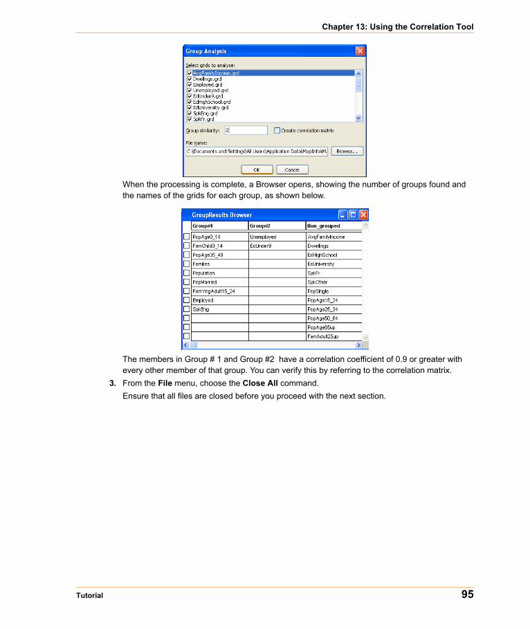
Chapter 13: Using the Correlation Tool
When the processing is complete, a Browser opens, showing the number of groups found and the names of the grids for each group, as shown below.
The members in Group # 1 and Group #2 have a correlation coefficient of 0.9 or greater with every other member of that group. You can verify this by referring to the correlation matrix.
3. From the File menu, choose the Close All command.Ensure that all files are closed before you proceed with the next section.
Tutorial 95

Performing a Predictive Analysis
Performing a Predictive AnalysisIn this exercise, you will learn how to analyze 24 grid layers of demographic data to determine other possible retail store locations. This will involve creating training regions around two successful stores and two less successful stores.
To create the regions:
1. Open the Predictive Analysis Map window located at the bottom of your screen.
2. Right-click the Map window, and choose the Layer Control command.
3. Enable the Editable check box for the Cosmetic Layer. Note the color of each symbol.
4. On the Drawing toolbar, click the Polygon button.5. Draw a polygon around each of the four symbols.
6. On the Drawing toolbar, click the Region Style button, and change the colour of the training regions to match the colour of the symbols. The green symbols represent the successful stores and the red symbols represent the less successful stores.
7. From the Map menu, choose the Save Cosmetic Objects command.8. In the Save Cosmetic Objects dialog box, choose New from the Transfer Cosmetic Objects to
Layer list, and click the Save button.9. In the Save Objects to Table dialog box, type "Training Regions" in the File Name box, and click
the Save button.
To assign a value to a region:
1. On the Main toolbar, click the Info button, and choose a region.2. In the Info Tool dialog box, type "1" for a green region and "2" for a red region.3. Repeat step 2 for all remaining regions.4. From the File menu, choose the Save Table command.
96 Tutorial
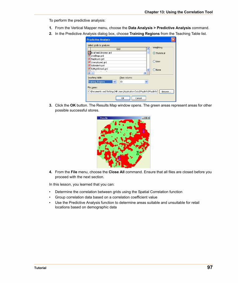
Chapter 13: Using the Correlation Tool
To perform the predictive analysis:
1. From the Vertical Mapper menu, choose the Data Analysis > Predictive Analysis command.2. In the Predictive Analysis dialog box, choose Training Regions from the Teaching Table list.
3. Click the OK button. The Results Map window opens. The green areas represent areas for other possible successful stores.
4. From the File menu, choose the Close All command. Ensure that all files are closed before you proceed with the next section.
In this lesson, you learned that you can:
• Determine the correlation between grids using the Spatial Correlation function• Group correlation data based on a correlation coefficient value• Use the Predictive Analysis function to determine areas suitable and unsuitable for retail
locations based on demographic data
Tutorial 97

Performing a Predictive Analysis
98 Tutorial

14
Splicing GridsAs a technician at a telecommunications company, you are evaluating the line of sight from the transmitters to the receiving antenna. The analysis involves an in-depth study of the elevation of the area. Ground elevation, height of buildings, and presence of vertical obstructions that can inhibit the transmissions must be considered. You will first determine the maximum heights of the terrain by merging a Digital Elevation Model with a file containing obstruction data, and then you will improve the accuracy of the data by stamping building information on the merged file.
In this lesson, you’ll learn:
Merging Two Grids . . . . . . . . . . . . . . . . . . . . . . . . . . . . . . . . . . . . .100Stamping Grids. . . . . . . . . . . . . . . . . . . . . . . . . . . . . . . . . . . . . . . .101Creating a Cross Section. . . . . . . . . . . . . . . . . . . . . . . . . . . . . . . .103
Required files can be found in:
• [User Data]\Tutorial\Lesson14
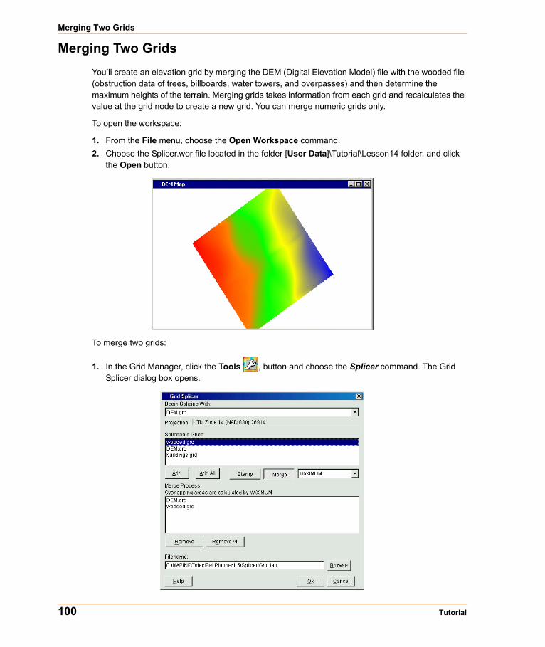
Merging Two Grids
Merging Two GridsYou’ll create an elevation grid by merging the DEM (Digital Elevation Model) file with the wooded file (obstruction data of trees, billboards, water towers, and overpasses) and then determine the maximum heights of the terrain. Merging grids takes information from each grid and recalculates the value at the grid node to create a new grid. You can merge numeric grids only.
To open the workspace:
1. From the File menu, choose the Open Workspace command. 2. Choose the Splicer.wor file located in the folder [User Data]\Tutorial\Lesson14 folder, and click
the Open button.
To merge two grids:
1. In the Grid Manager, click the Tools , button and choose the Splicer command. The Grid Splicer dialog box opens.
100 Tutorial
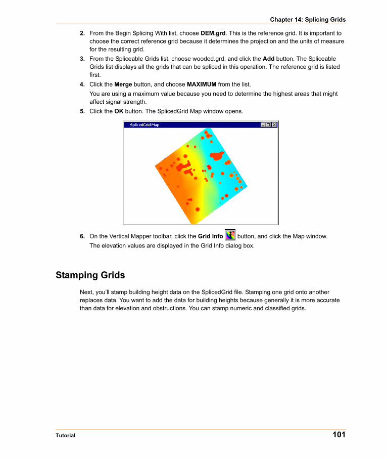
Chapter 14: Splicing Grids
2. From the Begin Splicing With list, choose DEM.grd. This is the reference grid. It is important to choose the correct reference grid because it determines the projection and the units of measure for the resulting grid.
3. From the Spliceable Grids list, choose wooded.grd, and click the Add button. The Spliceable Grids list displays all the grids that can be spliced in this operation. The reference grid is listed first.
4. Click the Merge button, and choose MAXIMUM from the list.You are using a maximum value because you need to determine the highest areas that might affect signal strength.
5. Click the OK button. The SplicedGrid Map window opens.
6. On the Vertical Mapper toolbar, click the Grid Info button, and click the Map window.The elevation values are displayed in the Grid Info dialog box.
Stamping GridsNext, you’ll stamp building height data on the SplicedGrid file. Stamping one grid onto another replaces data. You want to add the data for building heights because generally it is more accurate than data for elevation and obstructions. You can stamp numeric and classified grids.
Tutorial 101
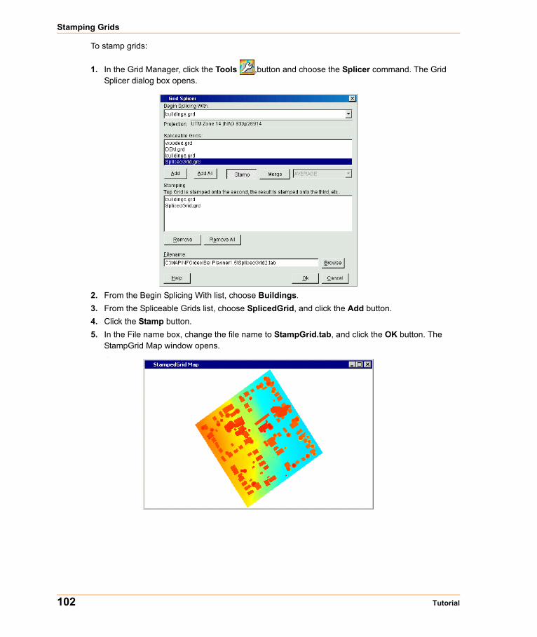
Stamping Grids
To stamp grids:
1. In the Grid Manager, click the Tools ,button and choose the Splicer command. The Grid Splicer dialog box opens.
2. From the Begin Splicing With list, choose Buildings.3. From the Spliceable Grids list, choose SplicedGrid, and click the Add button.4. Click the Stamp button.5. In the File name box, change the file name to StampGrid.tab, and click the OK button. The
StampGrid Map window opens..
102 Tutorial
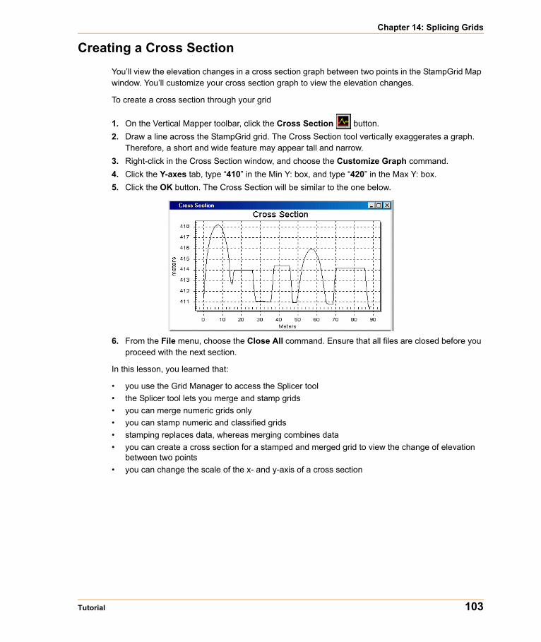
Chapter 14: Splicing Grids
Creating a Cross SectionYou’ll view the elevation changes in a cross section graph between two points in the StampGrid Map window. You’ll customize your cross section graph to view the elevation changes.
To create a cross section through your grid
1. On the Vertical Mapper toolbar, click the Cross Section button. 2. Draw a line across the StampGrid grid. The Cross Section tool vertically exaggerates a graph.
Therefore, a short and wide feature may appear tall and narrow.3. Right-click in the Cross Section window, and choose the Customize Graph command.4. Click the Y-axes tab, type “410” in the Min Y: box, and type “420” in the Max Y: box.5. Click the OK button. The Cross Section will be similar to the one below.
6. From the File menu, choose the Close All command. Ensure that all files are closed before you proceed with the next section.
In this lesson, you learned that:
• you use the Grid Manager to access the Splicer tool• the Splicer tool lets you merge and stamp grids• you can merge numeric grids only• you can stamp numeric and classified grids• stamping replaces data, whereas merging combines data• you can create a cross section for a stamped and merged grid to view the change of elevation
between two points• you can change the scale of the x- and y-axis of a cross section
Tutorial 103

Creating a Cross Section
104 Tutorial

15
Reclassing GridsAt times, you’ll need to reclassify or modify the class structure of a classified grid. In this exercise, you’ll reclassify the land use classes for Seattle so that all classes of the Tundra and the Perennial, Snow or Ice groups are combined into one group. You’ll rename a group, add new classes, and reassign classes from the original structure to the new structure.
In this lesson, you’ll learn how to
Reclassing a Classified Grid . . . . . . . . . . . . . . . . . . . . . . . . . . . . .106Reducing the Number of Classes . . . . . . . . . . . . . . . . . . . . . . . . .108
Required files can be found in:
• [User Data]\Tutorial\Lesson15
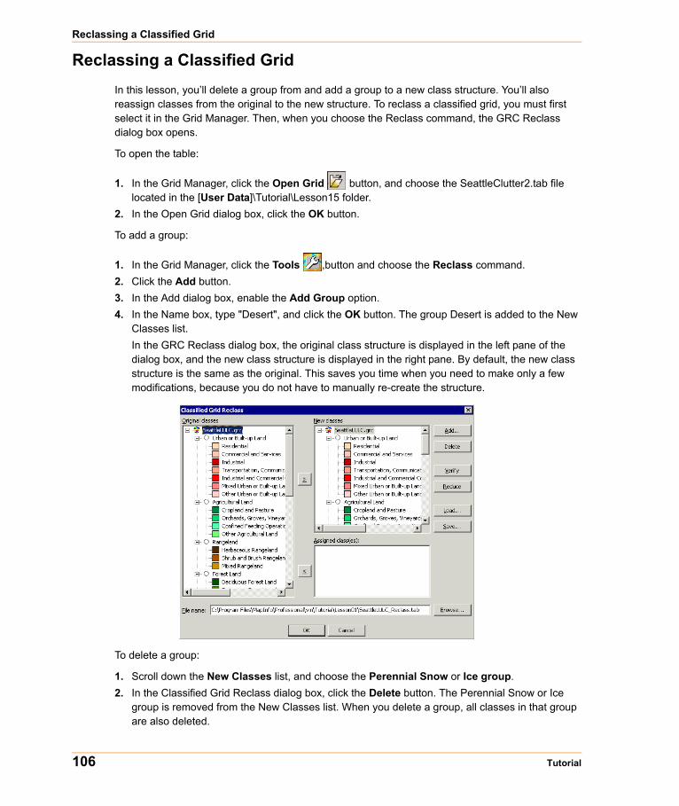
Reclassing a Classified Grid
Reclassing a Classified GridIn this lesson, you’ll delete a group from and add a group to a new class structure. You’ll also reassign classes from the original to the new structure. To reclass a classified grid, you must first select it in the Grid Manager. Then, when you choose the Reclass command, the GRC Reclass dialog box opens.
To open the table:
1. In the Grid Manager, click the Open Grid button, and choose the SeattleClutter2.tab file located in the [User Data]\Tutorial\Lesson15 folder.
2. In the Open Grid dialog box, click the OK button.
To add a group:
1. In the Grid Manager, click the Tools ,button and choose the Reclass command.2. Click the Add button.3. In the Add dialog box, enable the Add Group option.4. In the Name box, type "Desert", and click the OK button. The group Desert is added to the New
Classes list.In the GRC Reclass dialog box, the original class structure is displayed in the left pane of the dialog box, and the new class structure is displayed in the right pane. By default, the new class structure is the same as the original. This saves you time when you need to make only a few modifications, because you do not have to manually re-create the structure.
To delete a group:
1. Scroll down the New Classes list, and choose the Perennial Snow or Ice group.2. In the Classified Grid Reclass dialog box, click the Delete button. The Perennial Snow or Ice
group is removed from the New Classes list. When you delete a group, all classes in that group are also deleted.
106 Tutorial

Chapter 15: Reclassing Grids
To change the name of a group:
1. In the New Classes list, double-click Tundra.2. In the Add dialog box, type "Perennial, Snow and Ice" in the Name box, and click the OK
button.
To add classes to a group:
Before you can generate a grid based on the new class structure, you must reassign all the classes in the original structure to a group or class in the new structure.
1. From the New Classes list, choose the Perennial, Snow and Ice group, and click the Add button.
2. In the Add dialog box, choose the Add Class option, type "Perennial Snowfields" in the Name box, click the color swatch,
3. Choose a color, click the OK button.4. Click the OK button.5. Repeat step 2 to step 4 for the Glaciers class.
To move a class:
You can move the classes of the original structure to the new structure by dragging a class from the left pane into a class in the right pane. You cannot move a class to a group that contains no classes.
1. Choose the Perennial Snowfields class from the Original Classes list. 2. Click and drag it to the New Classes list, on top of the new Perennial Snowfields class. A triangle
is displayed beside Perennial Snowfields in the left pane.3. Move all classes from the Tundra and the Perennial Snow or Ice groups from the Original
Classes list to the new Perennial, Snow and Ice group in the New Classes list.4. Click the Verify button. A warning dialog box opens listing all unassigned classes. All classes in
the original grid must be assigned to a group or a class in the New Classes list before you can generate a grid based on the new class structure.
5. Assign the remaining classes of the original structure to the corresponding classes in the new structure.
6. Click the Verify button. 7. If any classes remain unassigned, assign them.
To reduce the new classes list:
The Desert group in the New Classes list that has no classes assigned to it. You can remove this group any other group that does not have classes assigned using the Reduce function.
• Click the Reduce button, and click the OK button.All groups that have no classes assigned are removed from the New Classes list. The SeattleClutter2_Reclass Map window opens.
Tutorial 107

Reducing the Number of Classes
Reducing the Number of ClassesIn this exercise, you will create a class structure that reduces the 37 classes of the SeattleClutter2 grid to eight classes. You will also save the new class structure, so that you can use it for the reclassification of other grids.
To reduce the number of classes:
1. In the Grid Manager, choose SeattleClutter2.grc, click the Tools button, and then choose the Reclass command.
2. In the New Class Structure dialog box, choose SeattleClutter2.grc, and click the Delete button.3. Click the Add button.4. In the Add dialog box, choose the Add Group option, type "Urban or Built-up Land", and
choose a color for the group.5. Repeat step 3 and step 4 to create the following groups:
• Agricultural Land• Rangeland• Forest Land• Water• Wetland• Barren Land• Perennial, Ice and SnowYou can now assign all of the classes in the Original Classes list to the corresponding class in the New Classes list.
6. Assign all of the classes from the Urban or Built-up Land group to the new Urban or Built-up Land class.
7. Repeat this for the remaining groups and classes.8. Click the Verify button.9. If no classes are unassigned, click the OK button.10. Click the Save button.11. In the File Name box, type "MYFirst.pfr".12. From the File menu, choose the Close All command. Ensure that all files are closed before you
proceed with the next section.
In this lesson, you learned that:
• you must choose a grid listed in the Grid Manager before you can reclass it• the new class structure mirrors the original class structure• you use the Add button to add groups and classes to the new class structure• you can remove a group or a class from the new structure using the Delete button• you can remove all empty groups and classes simultaneously using the Reduce button
108 Tutorial
16
Using the 3D View FunctionUsing the 3D GridView tool, you can create 3D renderings of numeric grids, turning an ordinary image into an impressive presentation aide.
In this lesson, you’ll learn:
Creating a 3D Grid . . . . . . . . . . . . . . . . . . . . . . . . . . . . . . . . . . . . .110Changing the Viewing Parameters . . . . . . . . . . . . . . . . . . . . . . . .112Setting the Light Source . . . . . . . . . . . . . . . . . . . . . . . . . . . . . . . .113Setting the Parameters for the Loaded Grid . . . . . . . . . . . . . . . .113Adding Layers . . . . . . . . . . . . . . . . . . . . . . . . . . . . . . . . . . . . . . . .114Adding Drapes . . . . . . . . . . . . . . . . . . . . . . . . . . . . . . . . . . . . . . . .116
Required files can be found in:• [User Data]\Tutorial\Lesson16 folder

Creating a 3D Grid
Creating a 3D GridGridView has many different settings that allow you to manipulate almost every aspect of a rendered scene.
To open the file:
1. From the File menu, choose the Open command.2. Choose the City.tab file located in the [User Data]\Tutorial\Lesson16 folder, and click the Open
button.
To create a 3D grid:
1. In the Grid Manager, click the 3D View button, and choose the Run 3D Viewer command. The Scene Properties dialog box opens.
2. Click the Cancel button. The GridView window opens.3. In the City - GridView dialog box, choose the Open Workspace command from the File menu.4. Choose the CityScape.gvw file located in the [User Data]\Tutorial\Lesson16 folder, and click the
Open button. A 3D image is displayed.
110 Tutorial
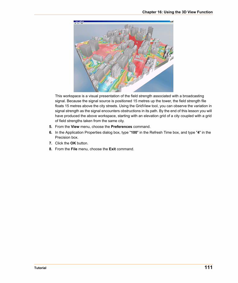
Chapter 16: Using the 3D View Function
This workspace is a visual presentation of the field strength associated with a broadcasting signal. Because the signal source is positioned 15 metres up the tower, the field strength file floats 15 metres above the city streets. Using the GridView tool, you can observe the variation in signal strength as the signal encounters obstructions in its path. By the end of this lesson you will have produced the above workspace, starting with an elevation grid of a city coupled with a grid of field strengths taken from the same city.
5. From the View menu, choose the Preferences command.6. In the Application Properties dialog box, type "100" in the Refresh Time box, and type "4" in the
Precision box.7. Click the OK button.8. From the File menu, choose the Exit command.
Tutorial 111

Changing the Viewing Parameters
Changing the Viewing ParametersTo change the viewing parameters
1. In the Grid Manager, click the 3D View button, and choose the Run 3D Viewer command. The Scene Properties dialog box opens.
The distance value in the Angle box is grayed out. In order to edit the distance from the grid to the camera, you must select the To Your Location option.
2. In the Set Viewing Mode section, choose the To Your Location option.3. In the Angle section, type “737” in the Distance box.4. In the Azimuth box, type “35”.5. In the Inclination box, type “38”. The Scene Properties dialog box will look as follows.
112 Tutorial

Chapter 16: Using the 3D View Function
Setting the Light SourceYou can set the properties of the light source on the Surface and Lighting tab. In the Lighting section:
• the Azimuth option controls the origin of the light source; 180 degrees indicates that the light is coming from true north
• the Inclination option controls the angle at which the light will shine on to the grid surface• the Specular option controls the amount of light that comes from a certain direction and bounces
off an object. Increasing specular light results in shiny spots and pronounced shadows.• the Diffuse light option controls unidirectional light that scatters uniformly in all directions when it
hits an object, resulting in shadow effects• the Ambient light option provides a source whose light rays are uniformly scattered throughout
the atmosphere, resulting in a bright scene without shadows
To set the light source:
1. In the Scene Properties dialog box, click the Surface and Lighting tab.2. In the Specular box, type “60”, in the Diffuse box, type “80”, and in the Ambient box, type “19”.3. In the Modeling dialog box, choose the Wireframe option.4. In the Scene dialog box, click the Backdrop Image button.5. Choose the CitySky.bmp file located in the [User Data]\Tutorial\Lesson16 folder, and click the
Open button.6. Enable the View Backdrop check box. The Scene Properties dialog box will look as follows.
Setting the Parameters for the Loaded GridYou can set the parameters for the loaded grid on the Loaded Grids tab. When you click on the tab, the title changes to the name of the grid selected in the Layer box. The grid’s z-values can be displayed in two modes:
• True Scale Mode uses the z-values of the grid to construct the graph. • Normalized Mode allows z-values that are in a different unit than the x- and y-values to be
normalized with respect to the grid’s width.
Tutorial 113
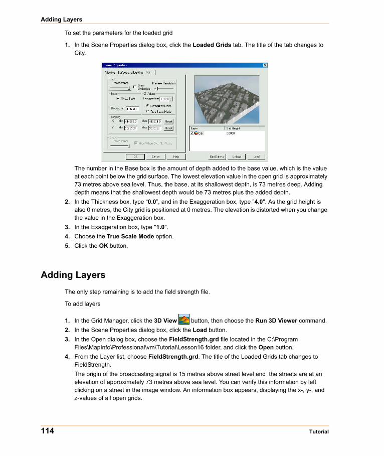
Adding Layers
To set the parameters for the loaded grid
1. In the Scene Properties dialog box, click the Loaded Grids tab. The title of the tab changes to City.
The number in the Base box is the amount of depth added to the base value, which is the value at each point below the grid surface. The lowest elevation value in the open grid is approximately 73 metres above sea level. Thus, the base, at its shallowest depth, is 73 metres deep. Adding depth means that the shallowest depth would be 73 metres plus the added depth.
2. In the Thickness box, type “0.0”, and in the Exaggeration box, type "4.0". As the grid height is also 0 metres, the City grid is positioned at 0 metres. The elevation is distorted when you change the value in the Exaggeration box.
3. In the Exaggeration box, type "1.0".4. Choose the True Scale Mode option.5. Click the OK button.
Adding LayersThe only step remaining is to add the field strength file.
To add layers
1. In the Grid Manager, click the 3D View button, then choose the Run 3D Viewer command.2. In the Scene Properties dialog box, click the Load button.3. In the Open dialog box, choose the FieldStrength.grd file located in the C:\Program
Files\MapInfo\Professional\vm\Tutorial\Lesson16 folder, and click the Open button.4. From the Layer list, choose FieldStrength.grd. The title of the Loaded Grids tab changes to
FieldStrength.The origin of the broadcasting signal is 15 metres above street level and the streets are at an elevation of approximately 73 metres above sea level. You can verify this information by left clicking on a street in the image window. An information box appears, displaying the x-, y-, and z-values of all open grids.
114 Tutorial
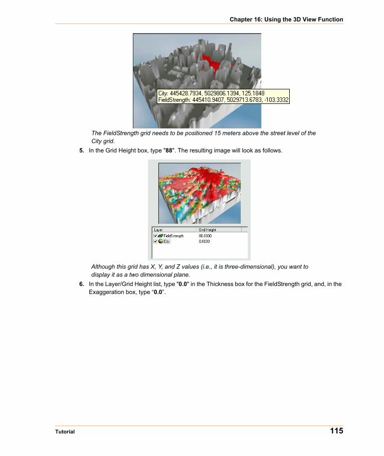
Chapter 16: Using the 3D View Function
The FieldStrength grid needs to be positioned 15 meters above the street level of the City grid.
5. In the Grid Height box, type "88". The resulting image will look as follows.
Although this grid has X, Y, and Z values (i.e., it is three-dimensional), you want to display it as a two dimensional plane.
6. In the Layer/Grid Height list, type "0.0" in the Thickness box for the FieldStrength grid, and, in the Exaggeration box, type “0.0”.
Tutorial 115
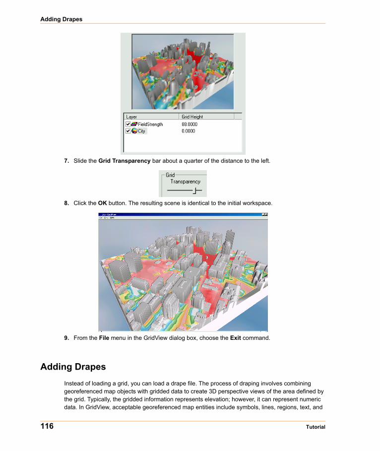
Adding Drapes
7. Slide the Grid Transparency bar about a quarter of the distance to the left.
8. Click the OK button. The resulting scene is identical to the initial workspace.
9. From the File menu in the GridView dialog box, choose the Exit command.
Adding DrapesInstead of loading a grid, you can load a drape file. The process of draping involves combining georeferenced map objects with gridded data to create 3D perspective views of the area defined by the grid. Typically, the gridded information represents elevation; however, it can represent numeric data. In GridView, acceptable georeferenced map entities include symbols, lines, regions, text, and
116 Tutorial

Chapter 16: Using the 3D View Function
other raster images such as aerial photos. Essentially, any map attribute that can be displayed in a MapInfo Map window can be included in a drape. If you want to drape other raster images, you should reproject the images to the same projection system as the grid they will be draped over.
To add a drape:
1. Right-click the Map window, and choose the Layer Control command.2. Add the FieldStrength grid to the City map window, making sure that FieldStrength is listed above
City.3. In the Grid Manager, choose City.grd. The drape file will have the same coordinate system as
the chosen grid.
4. Click the 3D View button, and choose the Make 3D Drape File command. An information dialog box opens, prompting you to select a map window.
5. Click in the FieldStrength grid window. The Drape File Resolution dialog box opens.
6. Click the OK button.7. In the Save Drape File As dialog box, click the Save button.
A message is displayed informing you that the drape has been created.
8. In the Grid Manager, choose City.grd, click the 3D View button, and choose the Run 3D Viewer command.
9. In the Scene Properties dialog box, choose the To Your Location option and type “737” in the Distance box.
10. Click the Loaded Grids tab, and choose the True Scale Mode option.11. Click the Load button.12. In the Open dialog box, change the file type to Drape Files (*.drp), and open FieldStrength.drp.13. In the Layer list in the Scene Properties dialog box, enable the check box next to the
FieldStrength drape.14. Click the OK button. The drape is displayed on the City grid. Instead of floating 15 metres above
the street level, the field strength information is now draped over the terrain.
Tutorial 117
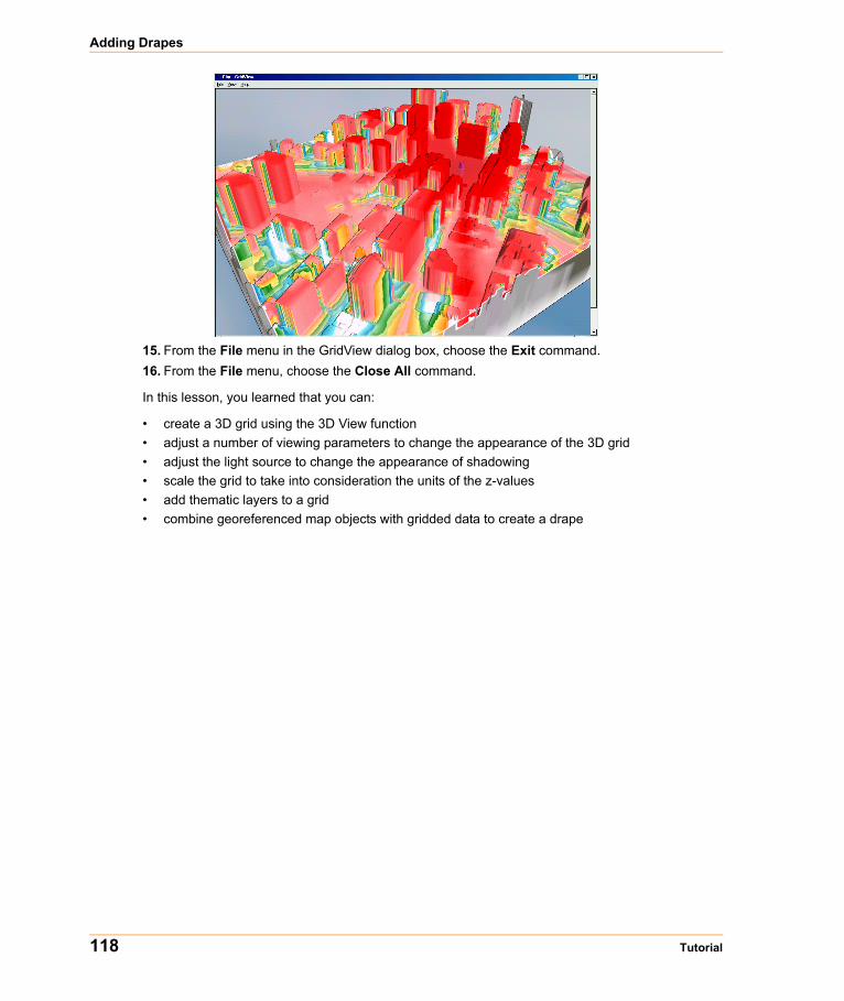
Adding Drapes
15. From the File menu in the GridView dialog box, choose the Exit command.16. From the File menu, choose the Close All command.
In this lesson, you learned that you can:
• create a 3D grid using the 3D View function• adjust a number of viewing parameters to change the appearance of the 3D grid• adjust the light source to change the appearance of shadowing• scale the grid to take into consideration the units of the z-values• add thematic layers to a grid• combine georeferenced map objects with gridded data to create a drape
118 Tutorial

Chapter 16: Using the 3D View Function
Tutorial 119

Index
Numerics3D grids
adding layers 114creating 110setting light source 113viewing parameters 112
CCalculator
converting units 70normalizing values 71saving expressions 72
Classified gridcontouring 55
Colour profilereversing 41
Commentssending 9
Complex viewshedsusing 60
Contourscreating 52, 55
Correlation analysis 92Correlation coefficient 92Correlation data
grouping 94Correlation matrix 93Cross Section
creating from line object 48from stamped grid 103
Customizingcross section graph 47
DData
aggregating 14inspecting 20making mappable 13
Documentation
updates 8Documentation set 8
user guides 8Drape
adding to 3D grid 116
GGraph
customizing cross section 47Grid Calculator 70Grid expression
creating 70Grid Info tool
using 23Grid query
multiple conditions 80simple 76two grids 78
Gridscreating 3D 110getting information on 23merging 100reclassing 106sloping 85, 100
Groupingcorrelation data 94
HHelp
accessing 8technical support 8
IInterpolation
Inverse Distance Weighting 32Natural Neighbour 27Rectangular 35
Intervisibilityalong existing line 64
Tutorial 120
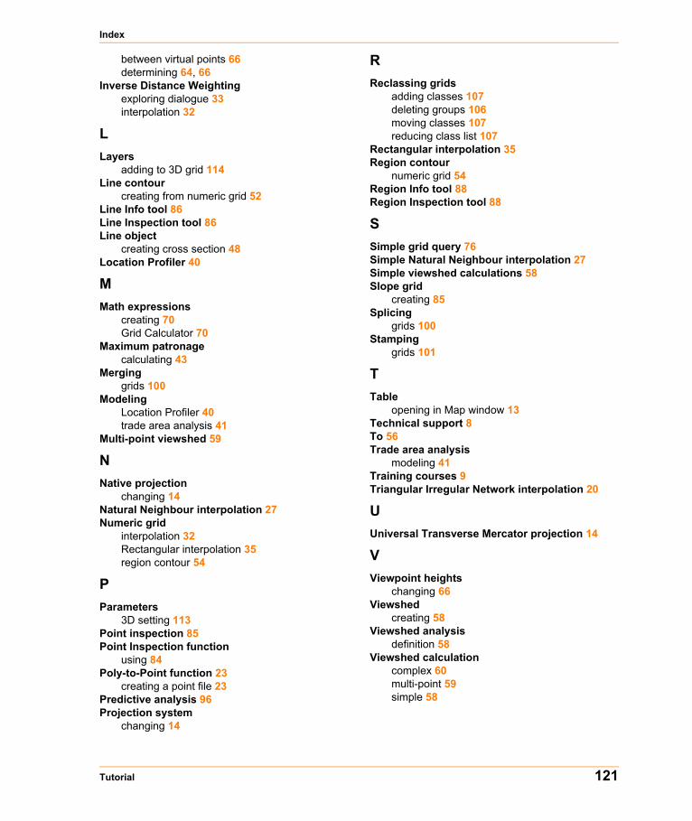
Index
between virtual points 66determining 64, 66
Inverse Distance Weightingexploring dialogue 33interpolation 32
LLayers
adding to 3D grid 114Line contour
creating from numeric grid 52Line Info tool 86Line Inspection tool 86Line object
creating cross section 48Location Profiler 40
MMath expressions
creating 70Grid Calculator 70
Maximum patronagecalculating 43
Merginggrids 100
ModelingLocation Profiler 40trade area analysis 41
Multi-point viewshed 59
NNative projection
changing 14Natural Neighbour interpolation 27Numeric grid
interpolation 32Rectangular interpolation 35region contour 54
PParameters
3D setting 113Point inspection 85Point Inspection function
using 84Poly-to-Point function 23
creating a point file 23Predictive analysis 96Projection system
changing 14
RReclassing grids
adding classes 107deleting groups 106moving classes 107reducing class list 107
Rectangular interpolation 35Region contour
numeric grid 54Region Info tool 88Region Inspection tool 88
SSimple grid query 76Simple Natural Neighbour interpolation 27Simple viewshed calculations 58Slope grid
creating 85Splicing
grids 100Stamping
grids 101
TTable
opening in Map window 13Technical support 8To 56Trade area analysis
modeling 41Training courses 9Triangular Irregular Network interpolation 20
UUniversal Transverse Mercator projection 14
VViewpoint heights
changing 66Viewshed
creating 58Viewshed analysis
definition 58Viewshed calculation
complex 60multi-point 59simple 58
Tutorial 121


![[Tutorial] Crop Daa Citra Satelit Menggunakan Global Mapper](https://img.pdfslide.us/doc/110x75/577c7b371a28abe054979067/tutorial-crop-daa-citra-satelit-menggunakan-global-mapper.jpg)