Application to the Waterview Connection Prepared for … · Application to the Waterview Connection Prepared for NZ Transport ... of Water & Atmospheric Research Ltd ... mean is based

25 June 2014 2.58 p.m.

A regression approach to assessing urban NO2 from passive monitoring

Application to the Waterview Connection

Prepared for NZ Transport Agency

June 2014

© All rights reserved. This publication may not be reproduced or copied in any form without the permission of the copyright owner(s). Such permission is only to be given in accordance with the terms of the client’s contract with NIWA. This copyright extends to all forms of copying and any storage of material in any kind of information retrieval system.

Whilst NIWA has used all reasonable endeavours to ensure that the information contained in this document is accurate, NIWA does not give any express or implied warranty as to the completeness of the information contained herein, or that it will be suitable for any purpose(s) other than those specifically contemplated during the Project or agreed by NIWA and the Client.

25 June 2014 2.58 p.m.

Authors/Contributors: Ian Longley Jennifer Gadd

For any information regarding this report please contact:

Ian Longley Air Quality Scientist Air Quality and Health +64-9-375 2096 [email protected]

National Institute of Water & Atmospheric Research Ltd

41 Market Place

Auckland Central 1010

Private Bag 99940

Newmarket

Auckland 1149

Phone +64-9-375-2050

Fax +64-9-375-2051

NIWA Client Report No: AKL-2014-023 Report date: June 2014 NIWA Project: NTA10101


25 June 2014 2.58 p.m.

Contents

Executive summary ..................................................................................................... 6

1 Introduction ........................................................................................................ 9

1.1 Background ................................................................................................. 9

1.2 Scope of the report .................................................................................... 10

2 Data used .......................................................................................................... 12

2.1 Data sources ............................................................................................. 12

2.2 Validity of data from passive monitoring .................................................... 12

3 Seasonal adjustment of monthly data ............................................................ 14

3.1 Seasonal patterns from long-term tube sites ............................................. 14

3.2 Monthly adjustment factors........................................................................ 14

3.3 How many months of data are required for a stable prediction of annual

mean? ....................................................................................................... 19

3.4 Validation against continuous data ............................................................ 21

3.5 Results of seasonal adjustment for NZTA Network sites in Auckland ........ 21

4 Empirical prediction of short-term impacts based on annual means ........... 22

4.1 Relationship between short and long-term impacts using ARC data .......... 22

4.2 Providing upper percentile NOx data for calculation of cumulative effects .. 24

5 The Spatial regression model.......................................................................... 25

5.1 Aims, approach and assumptions.............................................................. 25

5.2 Model derivation ........................................................................................ 26

5.3 Model results ............................................................................................. 27

5.4 Evaluating urban background using the regression model ........................ 29

5.5 Improving the regression model ................................................................ 30

6 Application of Regression Model to Waterview Project receptors ............... 31

6.1 Aims .......................................................................................................... 31

6.2 Results ...................................................................................................... 31

6.3 Cross-validation against dispersion modelling ........................................... 32

7 Recommendations for use in future assessments and feedback to

management of the NO2 Network .................................................................... 35

7.1 Scope of application .................................................................................. 35


25 June 2014 2.58 p.m.

7.2 Management of the NO2 Network .............................................................. 35

7.3 Potential other uses of the model and approach ........................................ 36

8 Acknowledgements .......................................................................................... 38

9 Glossary of abbreviations and terms .............................................................. 39

10 References ........................................................................................................ 40

Appendix A Estimated annual mean NO2 at passive monitoring sites in

Auckland .................................................................................................... 41

Appendix B Predicted baseline NO2 at the Waterview Connection project

assessment receptors ..................................................................................... 45

Tables

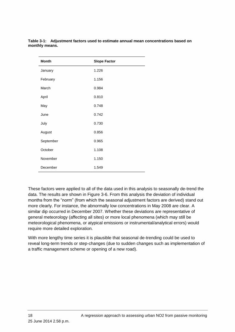
Table 3-1: Adjustment factors used to estimate annual mean concentrations based on monthly means. 18

Table 7-1: NZTA NO2 Network sites excluded from the spatial regression model. 36

Table B-1: Annual NO2 concentrations predicted for the Waterview Project assessment receptors using the spatial regression model. 45

Figures

Figure 2-1: Comparison of data from passive monitoring NO2 tubes with continuous monitoring (chemi-luminescence analyser) data from the MfE Gavin Street site. 13

Figure 2-2: Comparison of data from passive monitoring NO2 tubes with continuous monitoring data from the MfE Gavin Street site. 13

Figure 3-1: Regression plot of monthly January data versus 12-month rolling mean data for each site. 14

Figure 3-2: Regression plot of data versus 12-month rolling mean data for January to June. 16

Figure 3-3: Regression plot of monthly data versus 12-month rolling mean data for July to December. 16

Figure 3-4: Regression plot for January including data for highly trafficked sites. 17

Figure 3-5: Time series of monthly mean of all highly trafficked roadside and setback sites, and the difference between them. 17

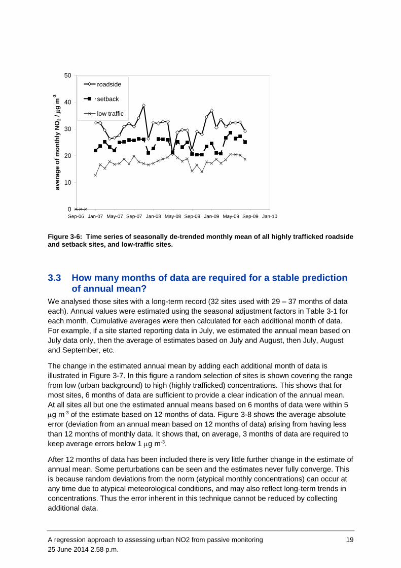
Figure 3-6: Time series of seasonally de-trended monthly mean of all highly trafficked roadside and setback sites, and low-traffic sites. 19

Figure 3-7: Annual averages based on 1 to 37 annual values calculated from monthly data. 20

Figure 3-8: Relationship between number of months of data upon which an estimated annual mean is based and the average absolute error in that estimate. 20

A regression approach to assessing urban NO2 from passive monitoring 5

25 June 2014 2.58 p.m.

Figure 3-9: Comparison of annual averages calculated from 24 hour averages, compared with annual averages calculated from adjusted monthly averages. 21

Figure 4-1: Empirical relationship between 99.9th percentile 1-hr NO2 concentrations and annual mean NO2 concentrations. 23

Figure 4-2: Empirical relationship between maximum 24-hr average NO2 concentrations and 99.9th percentile 1-hr NO2 concentrations. 23

Figure 4-3: Empirical relationship between 99.9th percentile 1-hr NO2 and NOx concentrations at ARC sites reporting >90% data coverage in any given year. 24

Figure 5-1: Initial results of plotting estimate annual mean NO2 at Auckland NZTA diffusion tube sites against traffic proximity factor. 28

Figure 5-2: Regression curves for ‘motorway’ and other sites. 29

Figure 6-1: Annual Mean NO2 concentrations (g m-3) at Waterview project assessment receptors, as predicted by the spatial regression model. 31

Figure 6-2: The road links explicitly modelled in the Waterview project dispersion modelling task, with the project assessment receptors shown in red. 32

Figure 6-3: Comparison between regression model and dispersion model (annual NO2 and 99.9th percentile 1 hour NOx respectively) for project assessment receptors. 33

Figure 6-4: Residual in the NO2 (regression) – NOx (dispersion) correlation as a function of distance of each receptor from its dominant road. 33

Figure 6-5: Improved relationship between annual mean NO2 (predicted by regression model) and peak NOx (predicted by dispersion model). 34

Figure A-1: Annual mean NO2 based on passive monitoring data in the north of Auckland. 41

Figure A-2: Annual mean NO2 based on passive monitoring data in the north west of Auckland. 42

Figure A-3: Annual mean NO2 based on passive monitoring data in the central isthmus of Auckland. 43

Figure A-4: Annual mean NO2 based on passive monitoring data in the southeast of Auckland. 44

Reviewed by Approved for release by

……………………………………… ……………………………… Formatting checked by ………………………………………


25 June 2014 2.58 p.m.

Executive summary In 2009 NIWA were commissioned to prepare material for the Air Quality Technical Report as

part of the Assessment of Environmental Effects for the SH20 Waterview Connection project,

including an analysis of baseline levels of nitrogen dioxide (NO2). NO2 is a significant

pollutant for road project assessment because it is the subject of a National Environmental

Standard (as well as other non-statutory Guidelines) and road vehicle emissions are its

dominant source. NO2 concentrations are known to be strongly elevated within tens of

metres of major roads.

It is common to assume that NO2 data from a conventional continuous monitoring site can be

considered representative of a wide area only if a significant degree of conservatism is

applied when analysing the data. The ‘margin of error’ applied can be highly arbitrary and

applied inconsistently. An alternative approach is to employ low-cost low-resolution passive

monitoring, although the data this provides cannot directly be used for comparison with the

Air Quality National Environmental Standard or Air Quality Guideline for NO2.

The SH20 Waterview Connection is a large road project for which a substantial network of

passive NO2 monitors were deployed across the project area, supplementing the NZTA NO2

Network (at the time of writing, there are 152 sites across Auckland). This network provided

an opportunity to develop a more sophisticated approach to baseline analysis for NO2 to

improve the accuracy in the assessment of current air quality and in particular the fine-scale

spatial variation across the project area.

In brief the approach consists of three components:

Seasonal adjustment factors to permit annual mean concentrations of NO2 to

be estimated from less than a year’s worth of monthly passive monitoring data.

A spatial correlation model (also known as a land-use regression model)

which predicts annual mean concentrations of NO2 at a given location as a

function of local spatial traffic data, initialised using passive monitoring data.

Empirical NO2-NOx relationships to predict short-term concentrations from

annual mean concentrations, for use in Cumulative impact analyses and

comparison with air quality Standards and Guidelines.

Analysis showed that for most sites, 6 months of data were sufficient to provide a confident

prediction of the annual mean. On average, 3 months of data were required to keep average

errors below 1 g m-3. The seasonal adjustment factors were validated by successfully

predicting annual means from monthly mean data gathered at 11 ARC continuous monitoring

sites.

Empirical relationships between short-term peak NO2 (and NOx) and long-term NO2

concentrations were derived from ARC (and NZTA) continuous monitoring data (12 sites in

total) from 1987 – 2008 inclusive:

99.9th percentile 1-hr NO2 = (2.31 x mean NO2) + 28

maximum 24-hr NO2 = (0.694 x 99.9th percentile 1-hr NO2) - 2.5

99.9th percentile 1-hr NO2 = (0.055 x 99.9th percentile 1-hr NOx) +37


25 June 2014 2.58 p.m.

We developed a spatial regression model to permit the information derived from passive

monitoring sites to be translated in space to nearby alternative sites (or receptors) within the

same general spatial domain. The resulting model is:

Annual mean NO2 (g m-3) = 0.00077(traffic proximity factor) + 10.4

Where traffic proximity factor = 20

0

65.0tancedisAADT

‘Distance’ is the shortest distance from the location of interest to a given road, and AADT is

the annual average daily traffic on that link. The traffic proximity factor is the sum of the

expression given for the 20 nearest road links. The power 0.65 is derived from NIWA’s

Roadside Corridor Model (Longley et al., 2010) and is representative of the long-term

average general rate of dilution of pollutants from a line source under Auckland meteorology.

The 10.4 represents the ‘urban background’ concentration, i.e. the concentration arising from

sources beyond the 20th nearest road link. Our analysis indicated that this value varied little

(if at all) across the area where most sites are located (principally around the SH16 Upgrade,

SH20 Waterview and SH20 Mt Roskill projects). More passive data from Auckland’s

periphery and CBD might confirm whether the background concentration reduces at the

urban edge, and/or increases in the CBD, and at what rate.

The general applicability of the model is dependent upon the existence of passive monitoring

data. Strictly the model derived can only be applied with confidence to areas around SH16

and SH20. The model’s performance in north, east and south Auckland, for instance, cannot

be specified due to the relative absence of monitoring sites in those areas. However, the

approaches demonstrated should apply generally to any urban area.

The regression model was used to predict annual mean NO2 at the 103 Waterview

Connection project assessment receptors. Predictions were compared with predictions of

99.9th percentile 1-hour NOx concentrations from dispersion modelling (conducted within the

Waterview project assessment). A strong correlation was observed (r2 = 0.87), especially

once an empirical correction factor was applied to account for differences in NO2/NOx ratio

with respect to distance from dominant roads. It was concluded that the regression model

and the dispersion model were in general agreement and are mutually supportive.

To apply the regression model elsewhere, passive monitoring sites must encompass a wide

range of AADT and distances to major roads, and more generally a wide range of traffic

intensities. For example, we recommend a variety of sites adjacent to minor roads, feeder

roads, major roads and arterial roads, plus a combination of areas of generally higher and

lower traffic density. To deploy a single urban background and single roadside site will not

give sufficient coverage to extend the model to a new area. For the purposes of project

assessment we recommend that urban background sites are especially useful. These are

sites which are fully embedded in the urban fabric (not at the urban periphery), but far from

major roads.

We suggest that the methods developed could also be used for other applications, such as

Health risk assessment

Emission trends assessment

8 A regression approach to assessing urban NO2 from passive monitoring

25 June 2014 2.58 p.m.

Management and rationalisation of the NO2 Network

Roadside corridor definition for mitigation and reverse sensitivity.


25 June 2014 2.58 p.m.

1 Introduction

1.1 Background

In 2009 NIWA were commissioned to prepare material for the Air Quality Technical Report as

part of the Assessment of Environmental Effects for the SH20 Waterview Connection project.

Broadly NIWA’s contribution consisted of three components:

Baseline analysis (i.e. assessment of current pre-project air quality),

Dispersion modelling (predicting the change in air quality attributable to the

project),

Cumulative analysis (the combined impact of the project and non-project

contributions to future air quality).

Baseline analysis conventionally relies on monitoring data from one, or a few sites which

may or may not be located for the purpose of project assessment, and which may or may not

be in locations representative of the impact of the project. NO2 is a significant pollutant for

road project assessment because it is the subject of a National Environmental Standard (as

well as other non-statutory Guidelines) and road vehicle emissions are its dominant source.

NO2 is mostly a ‘secondary’ pollutant which forms in the atmosphere through chemical

reaction of the primary pollutant nitric oxide (NO). This reaction is rapid but strongly

influenced by several factors including meteorological conditions. One consequence is that

NO2 concentrations are known to be strongly elevated within tens of metres of major roads.

The implication of all of these factors is that there is always significant uncertainty as to

whether any given monitor can represent concentrations of NO2 at other nearby locations.

Consequently, it is common to assume that data from a monitoring site can be considered

representative of a wide area only if a significant degree of conservatism is applied when

analysing the data. The ‘margin of error’ applied can be highly arbitrary and applied

inconsistently.

An alternative approach is to employ passive monitoring. Because of their low cost, passive

monitors can be deployed in dense networks across areas of interest. Their main limitation,

however, is that they report only a single concentration per deployment (usually 2 weeks or a

month). They also have a relatively low accuracy. This means that, although they can

provide an insight into spatial variation, they cannot be used for comparison with the AQNES

or AAQG (which are 1-hour and 24-hour average concentrations respectively). They can be

used to draw comparisons with the World Health Organisations’ annual guideline, but a

whole year’s worth of data is required. Even then, whether or not any given year is typical or

not is open to challenge. These factors have previously limited the use of passive monitoring.

Finally, the prediction of cumulative impacts requires the combination of the effect of project-

related emissions (usually expressed as oxides of nitrogen, or NOx – the sum of NO and

NO2) with the baseline (usually expressed as NO2 only) .The complex chemistry of NOx

means that NOx from emissions cannot simply be summed with baseline NO2. It is

advantageous if the baseline is also expressed in terms of NOx with the cumulative NOx

impact re-apportioned between NO2 and NO. Although all of this can, in principle, be


25 June 2014 2.58 p.m.

achieved with complex chemical-transport modelling, this approach is dependent upon (and

sensitive to) substantial amounts of data which are rarely available and is usually considered

too complex and uncertain for the purposes of a regulatory air quality assessment.

The SH20 Waterview Connection is a large, high-value and complex project. Before NIWA

began its assessment a substantial network of passive NO2 monitors were deployed by

NZTA across the project area, supplementing the then rapidly growing NZTA NO2 Network.

NIWA believed that this network provided an opportunity to develop a more sophisticated

approach to baseline analysis for NO2 which would help to overcome the problems discussed

above. The aim was to improve the accuracy in the assessment of current air quality and in

particular its fine-scale spatial variation across the area affected by the project.

In brief the approach consists of three components:

Seasonal adjustment factors to permit annual mean concentrations of NO2 to

be estimated from less than a year’s worth of monthly passive monitoring data.

A spatial correlation model (also known as a land-use regression model)

which predicts annual mean concentrations of NO2 at a given location as a

function of local spatial traffic data, initialised using passive monitoring data.

Empirical NO2-NOx relationships to predict short-term concentrations from

annual mean concentrations, for use in Cumulative impact analyses and

comparison with air quality Standards and Guidelines.

In the process of developing this new approach, further information and tools of more general

value has been derived regarding the influence of road traffic emissions on urban air quality.

1.2 Scope of the report

This report documents the approach taken to develop NO2 baseline data for the Waterview

project. It also briefly indicates other applications of the information and tools derived during

the development of the approach. These further applications could be developed more fully

in the future.

More specifically, it covers

The development of seasonal adjustment factors to estimate annual mean NO2

concentrations from monthly mean data.

A prototype empirical regression model which generalises the long-term spatial

distribution of air quality impacts from roads, as described by the NZTA NO2

network (currently Auckland only)

The use of this model to provide baseline NO2 (and NOx) data for the Waterview

project

Recommendations for how these approaches can be generalised (and

combined with other approaches) for other locations and other projects

It is important to note that this project is based on passive monitoring data as its main input.

The project scope did not include quality assurance or control of this data. It has been


25 June 2014 2.58 p.m.

assumed throughout that the data we have received from NZTA had already been through a

full QA/QC process.

It is our long-term intention that the approaches, methods and tools described in this report

are applicable nationwide. However, at present, the analysis is based solely on data from the

Auckland Region, and principally from areas around SH20 and SH16. The applicability of

results to other locations cannot, as yet, be assured.


25 June 2014 2.58 p.m.

2 Data used

2.1 Data sources

NZTA operate a nationwide monitoring network for NO2 using passive samplers. At the time

the analysis in this report was conducted (early 2010) there had been 152 sites established

at some time within the Auckland Region. Approximately 37 of these sites had been in

operation since 2007 and 34 further sites were added in April 2009. Further sites were added

in specific areas from July to October 2009: 16 sites around Te Atatu (July), 31 sites around

Waterview (September) and 25 sites around Massey (October). The locations of the sites are

shown in Appendix One.

Data from all Auckland sites from January 2007 to February 2010 were provided by NZTA.

2.2 Validity of data from passive monitoring

Passive samplers have been repeatedly deployed at several locations around Auckland

where NO2 is also monitored continuously using chemi-luminescence analysers (the method

required for monitoring compliance with the National Environmental Standards). One of

those sites is the MfE/ARC monitoring station at Gavin Street in Penrose, where passive

sampler tubes have been regularly installed in triplicate. Figure 2-1 shows the monthly

average NO2 from the continuous monitor compared to the monthly averages obtained from

the three passive samplers up to December 2009. Both methods follow the same trend over

time, with peak NO2 in June and low NO2 in December. A regression plot for the data

indicates that while there is considerable scatter in the data, there is a 1 to 1 relationship

between the two methods (slope of 0.9996). The passive samplers appear to measure 1 - 2

g m-3 higher than the continuous monitor.

This verification could not be repeated for other monitoring sites as passive samplers have

been installed only recently at most sites and there is a short temporal overlap.


25 June 2014 2.58 p.m.

Figure 2-1: Comparison of data from passive monitoring NO2 tubes with continuous monitoring (chemi-luminescence analyser) data from the MfE Gavin Street site.

Figure 2-2: Comparison of data from passive monitoring NO2 tubes with continuous monitoring data from the MfE Gavin Street site.

0

5

10

15

20

25

30

35

40

45

50

Jan-07 Mar-07 May-07 Jul-07 Sep-07 Nov-07 Jan-08 Mar-08 May-08 Jul-08 Sep-08 Nov-08

Mo

nth

ly a

ve

rag

e N

O2 (

g

m -3

)

AUC013 AUC014

AUC015 Average of 3 tubes

Continuous monitoring

y = 0.9996x + 1.6633

R2 = 0.7239

5

10

15

20

25

30

35

40

45

50

5 10 15 20 25 30 35 40

Monthly average NO2 from continuous monitoring ( g m-3

)

Mo

nth

ly a

ve

rag

e N

O2 f

rom

pa

ss

ive

sa

mp

lers

(

g m

-3)


25 June 2014 2.58 p.m.

3 Seasonal adjustment of monthly data

3.1 Seasonal patterns from long-term tube sites

Continuous monitoring of NO2, and previous analysis of passive monitoring of NO2 (ARC,

2007; Watercare, 2008, 2010) have shown that there is a strong and consistent seasonal

variation in concentrations in Auckland, with relatively elevated concentrations in winter.

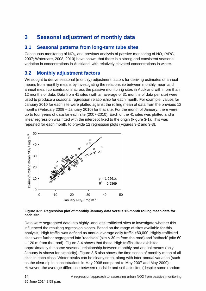
3.2 Monthly adjustment factors

We sought to derive seasonal (monthly) adjustment factors for deriving estimates of annual

means from monthly means by investigating the relationship between monthly mean and

annual mean concentrations across the passive monitoring sites in Auckland with more than

12 months of data. Data from 41 sites (with an average of 31 months of data per site) were

used to produce a seasonal regression relationship for each month. For example, values for

January 2010 for each site were plotted against the rolling mean of data from the previous 12

months (February 2009 – January 2010) for that site. For the month of January, there were

up to four years of data for each site (2007-2010). Each of the 41 sites was plotted and a

linear regression was fitted with the intercept fixed to the origin (Figure 3-1). This was

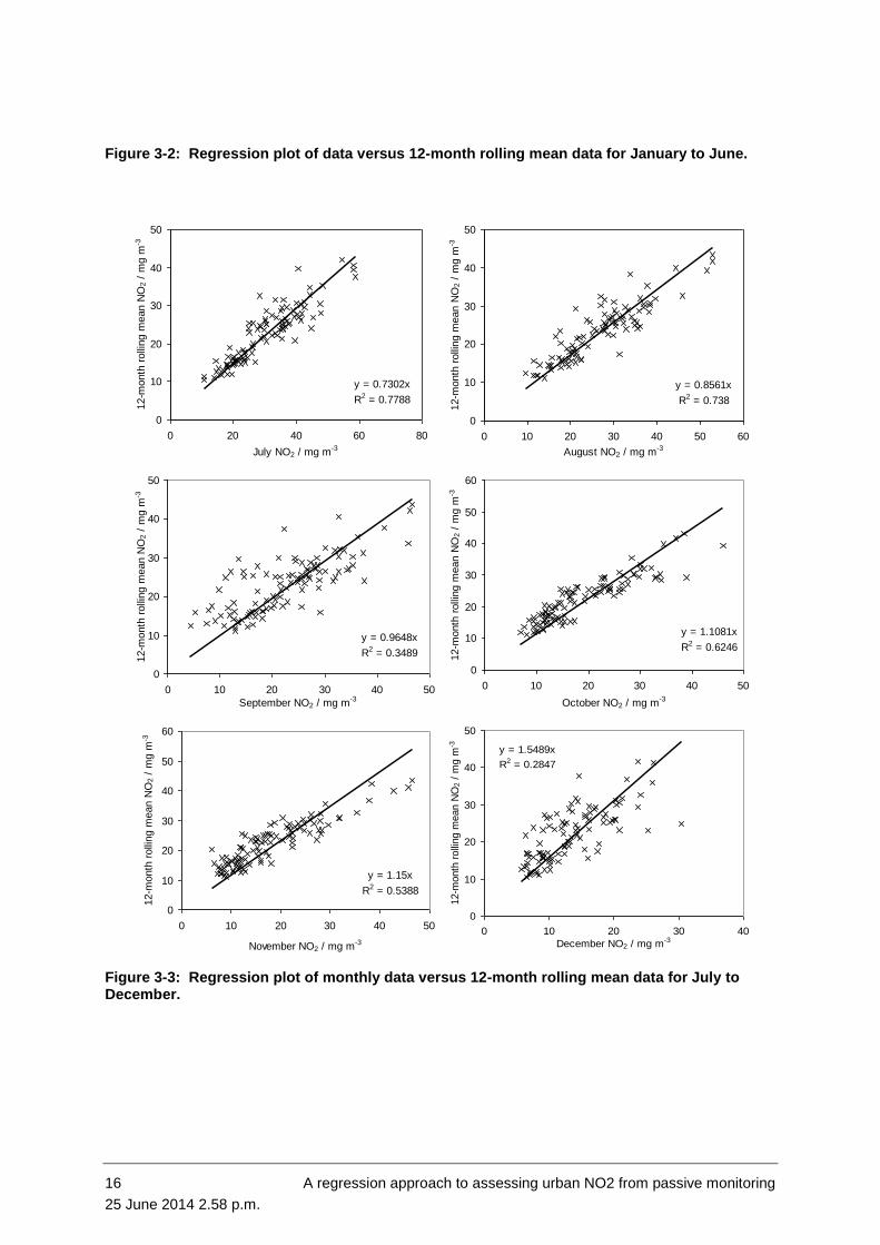
repeated for each month, to provide 12 regression plots (Figures 3-2 and 3-3).

Figure 3-1: Regression plot of monthly January data versus 12-month rolling mean data for each site.

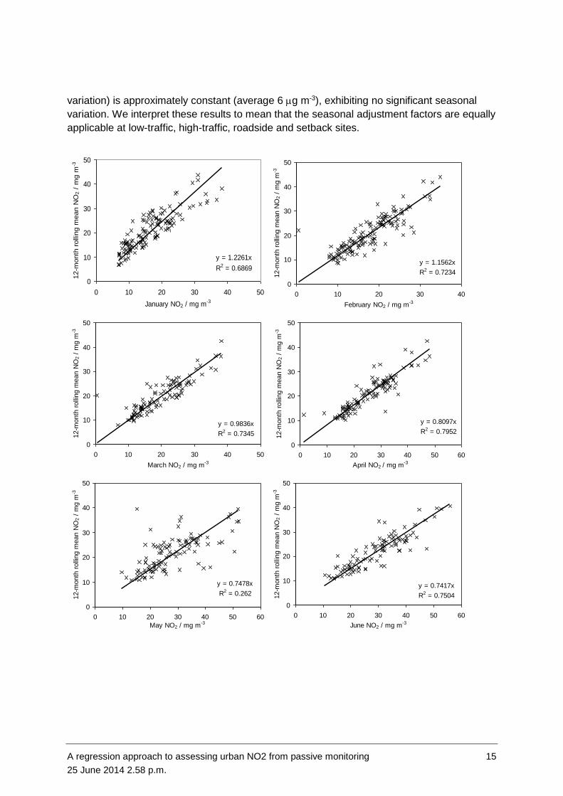
Data were segregated data into highly- and less-trafficked sites to investigate whether this

influenced the resulting regression slopes. Based on the range of sites available for this

analysis, ‘High traffic’ was defined as annual average daily traffic >60,000. Highly-trafficked

sites were further segregated into ‘roadside’ (site < 30 m from the road) and ‘setback’ (site 60

– 120 m from the road). Figure 3-4 shows that these ‘High traffic’ sites exhibited

approximately the same seasonal relationship between monthly and annual means (only

January is shown for simplicity). Figure 3-5 also shows the time series of monthly mean of all

sites in each class. Winter peaks can be clearly seen, along with inter-annual variation (such

as the clear dip in concentrations in May 2008 compared to May 2007 and May 2009).

However, the average difference between roadside and setback sites (despite some random

y = 1.2261x

R2 = 0.6869

0

10

20

30

40

50

0 10 20 30 40 50

January NO2 / mg m-3

12-m

onth

rolli

ng m

ean N

O2 /

mg m

-3

9


25 June 2014 2.58 p.m.

variation) is approximately constant (average 6 g m-3), exhibiting no significant seasonal

variation. We interpret these results to mean that the seasonal adjustment factors are equally

applicable at low-traffic, high-traffic, roadside and setback sites.

y = 1.2261x

R2 = 0.6869

0

10

20

30

40

50

0 10 20 30 40 50


12-m

onth

rollin

g m

ean N

O2 /

mg m

-3

9

y = 1.1562x

R2 = 0.7234

0

10

20

30

40

50

0 10 20 30 40

February NO2 / mg m-3

12-m

onth

rolli

ng m

ean N

O2 /

mg m

-3

y = 0.9836x

R2 = 0.7345

0

10

20

30

40

50

0 10 20 30 40 50

March NO2 / mg m-3

12-m

onth

rolli

ng m

ean N

O2 /

mg m

-3

y = 0.8097x

R2 = 0.7952

0

10

20

30

40

50

0 10 20 30 40 50 60

April NO2 / mg m-3

12-m

onth

rolli

ng m

ean N

O2 /

mg m

-3

y = 0.7478x

R2 = 0.262

0

10

20

30

40

50

0 10 20 30 40 50 60

May NO2 / mg m-3

12-m

onth

rolli

ng m

ean N

O2 /

mg m

-3

y = 0.7417x

R2 = 0.7504

0

10

20

30

40

50

0 10 20 30 40 50 60

June NO2 / mg m-3

12-m

onth

rolli

ng m

ean N

O2 /

mg m

-3


25 June 2014 2.58 p.m.

Figure 3-2: Regression plot of data versus 12-month rolling mean data for January to June.

Figure 3-3: Regression plot of monthly data versus 12-month rolling mean data for July to December.

y = 0.7302x

R2 = 0.7788

0

10

20

30

40

50

0 20 40 60 80

July NO2 / mg m-3

12-m

onth

rolli

ng m

ean N

O2 /

mg m

-3

y = 0.8561x

R2 = 0.738

0

10

20

30

40

50

0 10 20 30 40 50 60

August NO2 / mg m-312-m

onth

rolli

ng m

ean N

O2 /

mg m

-3

y = 0.9648x

R2 = 0.3489

0

10

20

30

40

50

0 10 20 30 40 50

September NO2 / mg m-3

12-m

onth

rolli

ng m

ean N

O2 /

mg m

-3

y = 1.1081x

R2 = 0.6246

0

10

20

30

40

50

60

0 10 20 30 40 50

October NO2 / mg m-3

12-m

onth

rolli

ng m

ean N

O2 /

mg m

-3

y = 1.15x

R2 = 0.5388

0

10

20

30

40

50

60

0 10 20 30 40 50

November NO2 / mg m-3

12-m

onth

rolli

ng m

ean N

O2 /

mg m

-3

y = 1.5489x

R2 = 0.2847

0

10

20

30

40

50

0 10 20 30 40

December NO2 / mg m-3

12-m

onth

rolli

ng m

ean N

O2 /

mg m

-3


25 June 2014 2.58 p.m.

Figure 3-4: Regression plot for January including data for highly trafficked sites.

Figure 3-5: Time series of monthly mean of all highly trafficked roadside and setback sites, and the difference between them.

The resulting regression slopes, or seasonal adjustment factors, are listed in Table 3-1. In

the absence of any evidence to the contrary we suggest that these factors apply at all sites in

Auckland.

0

10

20

30

40

50

0 10 20 30 40 50


12-m

onth

rolli

ng m

ean N

O2 /

mg m

-3

All sites

High traffic roadside

High traffic setback

0

10

20

30

40

50

Sep-06 Jan-07 May-07 Sep-07 Jan-08 May-08 Sep-08 Jan-09 May-09 Sep-09 Jan-10

ave

rag

e o

f m

on

thly

NO

2 /

g

m-3

roadside

setback

difference


25 June 2014 2.58 p.m.

Table 3-1: Adjustment factors used to estimate annual mean concentrations based on monthly means.

Month Slope Factor

January 1.226

February 1.156

March 0.984

April 0.810

May 0.748

June 0.742

July 0.730

August 0.856

September 0.965

October 1.108

November 1.150

December 1.549

These factors were applied to all of the data used in this analysis to seasonally de-trend the

data. The results are shown in Figure 3-6. From this analysis the deviation of individual

months from the “norm” (from which the seasonal adjustment factors are derived) stand out

more clearly. For instance, the abnormally low concentrations in May 2008 are clear. A

similar dip occurred in December 2007. Whether these deviations are representative of

general meteorology (affecting all sites) or more local phenomena (which may still be

meteorological phenomena, or atypical emissions or instrumental/analytical errors) would

require more detailed exploration.

With more lengthy time series it is plausible that seasonal de-trending could be used to

reveal long-term trends or step-changes (due to sudden changes such as implementation of

a traffic management scheme or opening of a new road).


25 June 2014 2.58 p.m.

Figure 3-6: Time series of seasonally de-trended monthly mean of all highly trafficked roadside and setback sites, and low-traffic sites.

3.3 How many months of data are required for a stable prediction of annual mean?

We analysed those sites with a long-term record (32 sites used with 29 – 37 months of data

each). Annual values were estimated using the seasonal adjustment factors in Table 3-1 for

each month. Cumulative averages were then calculated for each additional month of data.

For example, if a site started reporting data in July, we estimated the annual mean based on

July data only, then the average of estimates based on July and August, then July, August

and September, etc.

The change in the estimated annual mean by adding each additional month of data is

illustrated in Figure 3-7. In this figure a random selection of sites is shown covering the range

from low (urban background) to high (highly trafficked) concentrations. This shows that for

most sites, 6 months of data are sufficient to provide a clear indication of the annual mean.

At all sites all but one the estimated annual means based on 6 months of data were within 5

g m-3 of the estimate based on 12 months of data. Figure 3-8 shows the average absolute

error (deviation from an annual mean based on 12 months of data) arising from having less

than 12 months of monthly data. It shows that, on average, 3 months of data are required to

keep average errors below 1 g m-3.

After 12 months of data has been included there is very little further change in the estimate of

annual mean. Some perturbations can be seen and the estimates never fully converge. This

is because random deviations from the norm (atypical monthly concentrations) can occur at

any time due to atypical meteorological conditions, and may also reflect long-term trends in

concentrations. Thus the error inherent in this technique cannot be reduced by collecting

additional data.

0

10

20

30

40

50

Sep-06 Jan-07 May-07 Sep-07 Jan-08 May-08 Sep-08 Jan-09 May-09 Sep-09 Jan-10

ave

rag

e o

f m

on

thly

NO

2 /

g

m-3

roadside

setback

low traffic


25 June 2014 2.58 p.m.

Figure 3-7: Annual averages based on 1 to 37 annual values calculated from monthly data.

Figure 3-8: Relationship between number of months of data upon which an estimated annual mean is based and the average absolute error in that estimate.

10

20

30

40

50

Jan-

07

Mar

-07

May

-07

Jul-0

7

Sep-0

7

Nov

-07

Jan-

08

Mar

-08

May

-08

Jul-0

8

Sep-0

8

Nov

-08

Jan-

09

Mar

-09

May

-09

Jul-0

9

Sep-0

9

Nov

-09

Jan-

10

Cumulative average up to:

Es

tim

ate

d a

nn

ua

l a

ve

rag

e N

O2

AUC009 AUC010 AUC011 AUC012 AUC020 AUC023 AUC025 AUC026

Average values varying Average values stabilising

0.0

0.2

0.4

0.6

0.8

1.0

1.2

1.4

0 2 4 6 8 10 12 14

months of data available

ave

rag

e a

bs

olu

te e

rro

r in

esti

ma

ted

an

nu

al

mea

n /

g

m-3


25 June 2014 2.58 p.m.

3.4 Validation against continuous data

To verify the seasonal factor adjustment, we used the seasonal factors to predict annual

mean NO2 for data from ARC’s continuous monitoring data. 24 hour average NO2

concentrations were used to calculate monthly means, which were then adjusted using the

seasonal factors derived above to provide annual estimates. The mean of these annual

estimates was calculated for three individual years of monitoring (2006, 2007, 2008) and

compared to the annual mean for those years calculated directly from the 24 hour data.

This showed a clear correlation between the annual means based on seasonally adjusted

monthly means and those based on raw data (Figure 3-9).

Figure 3-9: Comparison of annual averages calculated from 24 hour averages, compared with annual averages calculated from adjusted monthly averages.

3.5 Results of seasonal adjustment for NZTA Network sites in Auckland

We applied the seasonal adjustment factors to all of the NZTA passive NO2 data provided to

us from Sep 2009 – Feb 2010 inclusive. The results are plotted on maps in Appendix One.

y = 0.9561x - 0.1865

R2 = 0.9979

0

5

10

15

20

25

30

35

40

45

50

0 10 20 30 40 50 60

Annual mean NO2 (from 24 hour average data)

An

nu

al

mean

NO

2 b

ased

on

ad

juste

d m

on

thly

avera

ges


25 June 2014 2.58 p.m.

4 Empirical prediction of short-term impacts based on annual means

4.1 Relationship between short and long-term impacts using ARC data

The chemical reactivity of nitrogen dioxide, and the complexity of the factors influencing its

short-term ambient concentration, means that concentrations are highly variable. Prediction

of NO2 concentrations is technically very demanding and inherently uncertain. On the other

hand, locations which are prone to high long-term concentrations (i.e. chronically highly

traffic-influenced locations) are also likely to be locations most likely to experience elevated

short-term concentrations due to the dominant role of local traffic emissions in ambient NO2

levels.

The approach to baseline analysis for NO2 is based on using passive monitoring data

reporting monthly mean concentrations, seasonally adjusted to estimate annual mean

concentrations. However, comparison with the AQNES and AAQG requires prediction of

peak 1-hour and 24-hour concentrations respectively. Strictly, peak (i.e. maximum) 1–hour

NO2 concentrations have been observed to be highly random short-lived events that are

unlikely to be generally representative of a site. Consequently, the convention is to assess

the 99.9th percentile as opposed to the true maximum, as representing the typical, repeatable

and representative peak NO2 concentration. This concept is also embedded in the National

Environmental Standard for NO2, which permits 9 exceedences per year – this equates to the

10th highest hourly concentration (approximately the 99.9th percentile) constituting a breach

of the Standard.

We compiled data from the Auckland Regional Council network of continuous NO2 monitors

to derive an empirical relationship between actual observed annual 99.9th percentile 1-hour

concentrations and the annual mean concentration for the same site for the same year. Data

has been incorporated from 1987 to 2008 inclusive. Data from 4 sites have been excluded

because the sites are thought to not be generally representative. Queen Street II is in a deep

CBD street canyon, whilst Khyber Pass Road is alongside a busy intersection with the

monitor inlet very close to a building façade. Both sites are subject to complex local air flows

such as recirculation which biases the data in certain wind conditions. Data from the Penrose

and Penrose IIA sites has also been excluded. These sites were deliberately placed in

industrial locations. Many industrial processes can emit large quantities of volatile organic

compounds which can locally promote the formation of NO2 in the atmosphere. Finally we

have also excluded data points in which a site reported less than 90 % data that year.

The resulting relationships are shown in Figure 4-1 and Figure 4-2. We have applied a least-

squares linear fit (three outliers seen in Figure 4-2 (circled) were not included in the

regression):

99.9th percentile 1-hr NO2 = (2.31 x mean NO2) + 28

maximum 24-hr NO2 = (0.694 x 99.9th percentile 1-hr NO2) - 2.5


25 June 2014 2.58 p.m.

Figure 4-1: Empirical relationship between 99.9th percentile 1-hr NO2 concentrations and annual mean NO2 concentrations. AC and NZTA sites reporting > 90% coverage per year.

Figure 4-2: Empirical relationship between maximum 24-hr average NO2 concentrations and 99.9th percentile 1-hr NO2 concentrations. AC and NZTA sites reporting >90 % coverage per year.

0

20

40

60

80

100

120

0 5 10 15 20 25 30 35

annual mean NO2 / g m-3

99.9

th p

erc

en

tile

1-h

r m

ean

NO

2 /

g

m-3

Mount Eden II (A)

Penrose II (B)

Mount Eden II (B)

Takapuna

Henderson

Kingsland

Glen Eden

Patumahoe

Pukekohe

Warkworth

Alan Wood Reserve

Cowley Street

y = 0.694x - 2.458

0

10

20

30

40

50

60

70

80

90

100

0 50 100 150 200

99.9th percentile 1-hr NO2 / g m-3

maxim

um

24-h

r avg

NO

2 /

g

m-3

Mount Eden II (A)

Penrose II (B)

Mount Eden II (B)

Takapuna

Henderson

Kingsland

Glen Eden

Patumahoe

Warkworth

Series1

Linear (Series1)


25 June 2014 2.58 p.m.

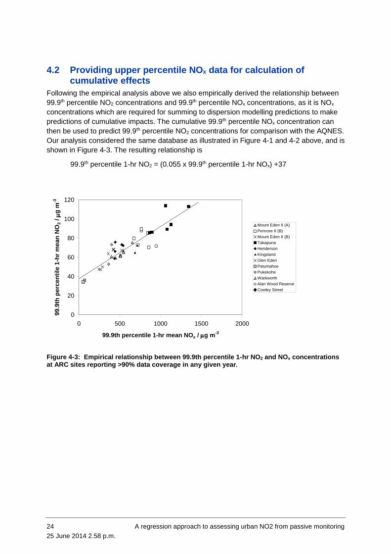
4.2 Providing upper percentile NOx data for calculation of cumulative effects

Following the empirical analysis above we also empirically derived the relationship between

99.9th percentile NO2 concentrations and 99.9th percentile NOx concentrations, as it is NOx

concentrations which are required for summing to dispersion modelling predictions to make

predictions of cumulative impacts. The cumulative 99.9th percentile NOx concentration can

then be used to predict 99.9th percentile NO2 concentrations for comparison with the AQNES.

Our analysis considered the same database as illustrated in Figure 4-1 and 4-2 above, and is

shown in Figure 4-3. The resulting relationship is

99.9th percentile 1-hr NO2 = (0.055 x 99.9th percentile 1-hr NOx) +37

Figure 4-3: Empirical relationship between 99.9th percentile 1-hr NO2 and NOx concentrations at ARC sites reporting >90% data coverage in any given year.

0

20

40

60

80

100

120

0 500 1000 1500 2000

99.9th percentile 1-hr mean NOx / g m-3

99.9

th p

erc

en

tile

1-h

r m

ean

NO

2 /

g

m-3

Mount Eden II (A)

Penrose II (B)

Mount Eden II (B)

Takapuna

Henderson

Kingsland

Glen Eden

Patumahoe

Pukekohe

Warkworth

Alan Wood Reserve

Cowley Street


25 June 2014 2.58 p.m.

5 The Spatial regression model

5.1 Aims, approach and assumptions

5.1.1 The need for the model

It has been described in the preceding chapters how monthly mean concentrations derived

from passive monitoring can be used to predict annual means and peak short-term means

(1-hour and 24-hour averages) by applying empirically derived formulae. However, in the

case of project assessment it is quite likely that passive monitoring sites do not cover all of

the project assessment receptors, nor are co-located with them. This was certainly the case

in the Waterview Connection project. Whereas small spatial deviations in location between

monitoring and receptor are commonly accepted, and may be acceptable for PM10, the sharp

spatial gradients in NO2 around roads means that relatively small displacements could lead

to large errors in predicted NO2 concentrations.

5.1.2 The purpose of the model

We chose to develop a spatial regression model to permit the information derived from

passive monitoring sites to be translated in space to nearby alternative sites (or receptors)

within the same general spatial domain. Specifically, the model empirically relates annual

mean NO2 (derived from passive monitoring either directly or by seasonal adjustment of

monthly means) to geographical variables relating to the passive monitoring site. The

resulting regression model will then predict annual NO2 for another site using that site’s

variable values. The approach is equivalent to land-use regression models, which have been

widely used elsewhere, particularly for population exposure assessment for health-effects

studies (Hoek et al., 2008). However, we have chosen not to use the term ‘land-use’ as our

model does not rely on what is generally considered to be ‘land-use’ data, but instead relies

on roads and traffic data (see below).

5.1.3 Anticipated explanatory variables

Land-use regression models have been developed for many cities around the world,

incorporating a range of explanatory variables (see the review by Hoek et al., 2008.). Our

aim was to keep the number of variables to a minimum. It was also our intention to permit for

the future transferability of the model to other parts of Auckland and to other cities in New

Zealand. This implies a need to minimise the number of explanatory variables. It was also a

requirement that the variables chosen should be easily obtainable from readily available data

sources.

Our initial choice was to include three factors:

annual average daily traffic on nearby roads

distance to nearby roads

background factors.

The background component represents sources beyond the nearby roads. It could also

represent urban density (as a proxy for traffic density on a ~km2 scale or larger). The

background component might be expected to reduce at the urban periphery and in low/no

emission locations such as the harbours, parks, etc.


25 June 2014 2.58 p.m.

5.2 Model derivation

5.2.1 Model formulation

A trial version of the model was developed based on the assumption:

NO2 = f(background, AADT on nearest major road, 1/√distance to nearest major road).

The trial version gave encouraging results, but highlighted the need to deal with the AADT

and distance to multiple roads in urban settings.

After the trial version, all further model development was conducted using ArcGIS to

generate independent variables as input to the model. We firstly used GIS functionality to

systematically extend the search for nearby traffic data to the nearest 20 road links. In doing

so we potentially captured some of the background component also.

The first version of the model was formulated as follows:

NO2 = traffic proximity factor + residual

Where traffic proximity factor = 20

0

65.0tancedisAADT

The distance is the shortest distance to the road link. The power 0.65 is derived from NIWA’s

Roadside Corridor Model (Longley et al., 2010) and is representative of the long-term

average general rate of dilution of pollutants from a line source under Auckland meteorology.

A sensitivity analysis confirmed that this value gave a better performing model than one

based on the powers 0.33, 0.5 and 1 (cube root, square root and linear-inverse,

respectively). The nature of the residual was left unspecified until the first (traffic) term had

been evaluated.

5.2.2 Traffic/road data

The road link and traffic data used for the derivation of the spatial regression model was

provided to NIWA for the purposes of the Waterview Connection assessment. The data was

provided as a single shape file and represented the project’s 2006 scenario. The traffic data

was derived from the ART3 model and contained AADT for both directions (each direction

constituting one road link).

This data was not ideal for the purposes of constructing the regression model for the

following reasons:

Being representative of 2006, the file did not include the SH20 Mt Roskill

Extension or the Albany-Greenhithe section of the SH18 Upper Harbour

Highway. Both roads were recently opened and some of the passive monitoring

data comes from sites next to these two roads. We would therefore not expect

this data to be correlated with traffic on roads that do not exist in the traffic file.

The original purpose of the shape file was for traffic modelling. One implication

was that the location of the road links was indicative rather than geographically

accurate, leading to some errors in alignment.

Some minor roads were missing.


25 June 2014 2.58 p.m.

In May 2010, Beca Infrastructure was able to supply NIWA with geographically-accurate

replacement shape file data for a 1 km corridor surrounding SH16 from Te Atatu to the

Central Motorway Junction.

5.2.3 GIS analysis

A script was written for use in ArcGIS to evaluate the traffic proximity factor for a given list of

co-ordinates. The script conducted a search for the 20 nearest road links to the given co-

ordinates evaluated by the shortest direct distance.

The co-ordinates of the NZTA NO2 Network sites in Auckland were provided as input. The

traffic proximity factor for each site was calculated using Microsoft Excel.

5.2.4 Implications of searching for 20 nearest links

By specifying that the analysis should seek the 20 nearest links we found that the search

extended 214 m on average, up to a maximum of 511 m (with one exception – site AUC040

located in Greenhithe, from which the 20th nearest link was nearly 1 km away).

We compared the implications of searching for 20 links rather than 10. For 84 % of the tube

sites, including the 10 more distant links increase the traffic proximity factor by less than 20

%, and for half of the sites the increase was less than 7 %. Thus decreasing the links from 20

to 10 would have a relatively minor effect in most cases. However, for the remaining 16 % of

sites, the extra 10 links increase the traffic proximity factor by 20 – 50 %. There was no clear

common characteristic to these more-affected sites, although 5 were clearly in more

peripheral locations (Glen Eden, Westgate, Albany) than most sites.

Although further research is justified in considering the implications of the number of links

chosen for the search process, we chose to proceed with 20 as this involved no significant

further processing time compared to 10.

5.3 Model results

Figure 5-1 shows the initial results of annual mean NO2 concentration for all of the NZTA NO2

Network sites (data based on seasonal adjustment of data from September 2009 to February

2010 inclusive) plotted against the traffic proximity factor (based on 20 nearest links). The

sites have been allocated to several groups as follows:

Several sites alongside the busiest sections of SH1 (from Sulphur Beach Rd,

north of the Harbour Bridge to Gavin Street in Penrose) were found to exhibit

slightly lower NO2 per traffic proximity factor than other sites

Several sites alongside SH16 (near the Pt Chevalier/Great North Road and Te

Atatu Road interchanges) were found to exhibit slightly lower NO2 per traffic

proximity factor than other sites

Those sites in very close proximity to intersections exhibited significant scatter.

Several sites were affected by alignment or missing link errors in the traffic

shape file and many of these sites were outliers in Figure 5-1.

Sites around SH16 in Massey were subject to shape file alignment errors and

missing links.


25 June 2014 2.58 p.m.

Data near SH20 Mt Roskill have been segregated due to the motorway not

appearing in the 2006 traffic data leading to an under-estimate of traffic

proximity factor.

A few other sites were segregated due to other recent traffic changes

(construction work on Manukau Harbour Crossing, opening of Upper Harbour

Highway), complex terrain or roadway/site elevation (which introduces error in

calculating distance).

Three further sites were removed due to NO2 values that did not appear to be

credible (too high or low for their respective sites).

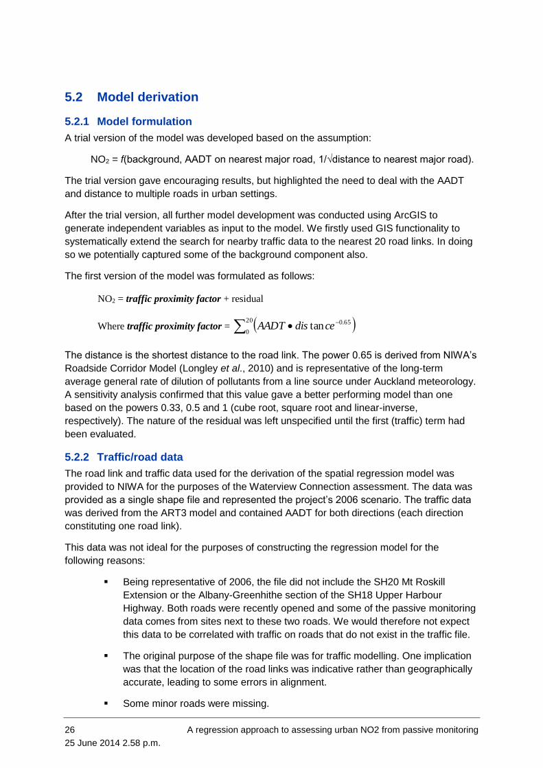
For all 45 remaining sites a best fit linear regression (r2 = 0.84) was found:

Annual mean NO2 = (0.00077 x traffic proximity factor) + 10.4

Figure 5-1: Initial results of plotting estimate annual mean NO2 at Auckland NZTA diffusion tube sites against traffic proximity factor. White = sites excluded from regression model, grey = motorway sites, black = all other sites.

Until the shape file errors can be resolved, and current traffic data provided for the SH20 Mt

Roskill Extension, we have discarded sites from Massey, Mt Roskill, and others with links

errors. Furthermore we have discarded intersection sites at the expense of limiting the model

to not be applicable at intersections. This was appropriate in the case of the Waterview

project as no receptors were located at intersections. Furthermore, we have clustered the

SH1 and SH16 (Te Atatu and Pt Chevalier) sites together to form a cluster of ‘motorway’

sites. However, it must be noted that, at this time, the ‘motorway’ cluster does not include

motorway sites at other locations (e.g. SH1 Northern Motorway, other than Sulphur Beach

Road, and SH1 Southern Motorway south of Penrose, or SH16 west of Te Atatu and east of

Pt Chevalier). Further research is justified into whether a separate ‘motorway’ cluster is

necessary and what physical explanation might justify it.

y = 0.0008x + 10.402

R2 = 0.8394

0

5

10

15

20

25

30

35

40

45

50

0 10000 20000 30000 40000 50000 60000 70000

traffic proximity factor

an

nu

al

me

an

NO

2 /

g

m-3

included

SH1

Pt Chev

Te Atatu

intersection

links error

Massey

Mt Roskill

others

Linear (included)


25 June 2014 2.58 p.m.

The resulting regression is displayed in Figure 5-2. The regression for the motorway sites (of

which there are 18) is

Annual mean NO2 = (0.00064 x traffic proximity factor) + 9.3

Figure 5-2: Regression curves for ‘motorway’ and other sites.

5.4 Evaluating urban background using the regression model

It was noted above that we developed a model of the form

NO2 = traffic proximity factor + residual

With an assumption that the residual would likely represent the ‘background’, i.e.

concentrations due to sources other than the nearby roads, and that this background may or

may not possess a degree of spatial variation. It can be seen from Figures 5-1 and 5-2 that

the model indicated a residual of approximately 10 g m-3 (the y-axis intercept). As this value

is well-defined we conclude that there is no discernible spatial variation in the residual (and

hence background) in this dataset.

It must be borne in mind that the ability of the model to detect a variation in the background is

in part dependent upon the monitoring sites actually encompassing locations which would

reveal such a variation. Not shown in Figures 5-1 and 5-2 are data from the passive monitors

co-located with ARC’s Glen Eden monitoring station. This site is towards the urban periphery

and far from any major roads. The estimated annual mean NO2 at these sites is 7 – 8 g m-3.

More passive data from the urban periphery might confirm whether the background

concentration does indeed reduce at the urban edge, and at what rate. However, for the

purposes of the Waterview project, this analysis strongly supports the assumption that urban

background NO2 is 10.4 g m-3 across the project area.

y = 0.0008x + 10.402

R2 = 0.8394

y = 0.0006x + 9.3294

R2 = 0.8738

0

5

10

15

20

25

30

35

40

45

50

0 10000 20000 30000 40000 50000 60000 70000

traffic proximity factor

an

nu

al

mean

NO

2 /

g

m-3

motorway

other

Linear (other)

Linear (motorway)


25 June 2014 2.58 p.m.

5.5 Improving the regression model

The next step in developing the regression model is to re-evaluate the model with fully

geographically accurate road/traffic shape files. Small improvements should be gained from

incorporating road/traffic data for new links opened since 2006 (such as SH20 Mt Roskill

Extension).

The general applicability of the model is dependent upon the passive monitoring sites from

which input data is available. The model’s performance in east Auckland, for instance,

cannot be specified due to the general absence of sites in that area.


25 June 2014 2.58 p.m.

6 Application of Regression Model to Waterview Project receptors

6.1 Aims

We used the regression model developed in chapter 5 (non-motorway formulation) to predict

annual mean NO2 at the 103 Waterview Connection project assessment receptors (the

receptor locations are shown in Figure 6-1). This involved running the GIS script to search for

the 20 nearest links to the receptors to calculate the traffic intensity factor for each. The

same 2006 traffic shape file was used as described above.

During the dispersion modelling for the Waterview Connection, the co-ordinates of the

assessment receptors had been adjusted to account for alignment errors in the traffic shape

file. We used the same adjusted co-ordinates in this exercise.

6.2 Results

The full set of predictions of annual NO2 concentrations at the project receptors is provided in

Appendix Two. They are also plotted on a map in Figure 6-2.

N.B: It is important to note that the spatial regression model was based on 2006 traffic data,

and does NOT therefore, include the SH20 Mt Roskill Extension. Hence predictions close to

that motorway are likely to be under-predictions of concentrations relative to those measured

in the area by passive monitoring which was installed after the motorway opened.

Figure 6-1: Annual Mean NO2 concentrations (g m-3) at Waterview project assessment receptors, as predicted by the spatial regression model.


25 June 2014 2.58 p.m.

6.3 Cross-validation against dispersion modelling

A degree of confidence in the results of the spatial regression model can be gained by

comparing the results with those from the Waterview project dispersion modelling. That

dispersion modelling predicted the 99.9th percentile 1-hour NOx concentration (for the

assessment year of 2007) arising from vehicle emissions on local roads only. The roads

modelled are shown in Figure 6-2. The regression model seeks to do a very similar thing, i.e.

assess the contribution from local roads only (the nearest 20, i.e. up to 214 m away on

average). Although the dispersion model predicts NOx and the regression model NO2, we

might expect them to give reasonably correlated results given that, in the long-term, NOx and

NO2 are reasonably well correlated (see Figures 4-1 and 4-3). The correlation might break

down towards the edge of the emission modelling domain (i.e. the roads whose emissions

were explicitly modelled).

Figure 6-2: The road links explicitly modelled in the Waterview project dispersion modelling task, with the project assessment receptors shown in red.

Figure 6-3 shows the result of the regression model predictions plotted against the dispersion

model predictions. There appears to be a reasonable linear relationship (r2 = 0.68).


25 June 2014 2.58 p.m.

Figure 6-3: Comparison between regression model and dispersion model (annual NO2 and 99.9th percentile 1 hour NOx respectively) for project assessment receptors.

We applied a least-squares linear fit and calculated the residual. There appeared to be a

relationship between the residual and the distance of the receptor to the ‘dominant’ local road

(Figure 6-4). The ‘dominant’ local road was defined as the road link making the largest

contribution to the traffic proximity factor (i.e. the link with the largest value of AADT x

distance-0.65). There may be some error in identifying this link, and the links chosen have not

been independently verified. This may account for the outliers seen in Figure 6-4.

Figure 6-4: Residual in the NO2 (regression) – NOx (dispersion) correlation as a function of distance of each receptor from its dominant road.

y = 0.017x + 10.297

R2 = 0.6798

0

5

10

15

20

25

30

0 200 400 600 800 1000

99.9th percentile NOx (dispersion model) / g m-3

an

nu

al

mea

n N

O2 (

reg

res

sio

n m

od

el)

/

g

m-3

y = -0.0057x + 0.7052

-6.0

-4.0

-2.0

0.0

2.0

4.0

6.0

0 200 400 600 800

distance to dominant road / m

reg

ress

ion

mo

de

l re

sid

ua

ls

outliers

receptors

Linear (receptors)


25 June 2014 2.58 p.m.

We derived a correction to account for this relationship:

Correction to annual NO2 = (-0.0057 x distance to dominant road) +0.71

The ‘corrected’ NO2 values are re-plotted against dispersion model NOx in Figure 6-5. A

strong correlation is seen with r2 = 0.87. Thus, we can conclude that the regression model

and the dispersion model are in general agreement and are mutually supportive.

Figure 6-5: Improved relationship between annual mean NO2 (predicted by regression model) and peak NOx (predicted by dispersion model).

It is beyond the scope of this research at present to explain or provide a physical

interpretation of the distance-related correction derived above. However, it is generally

known that the NO2/NOx ratio is related to distance to emission source in the long-term. We

believe that further research is justified to investigate the cause and nature of these

relationships.

y = 0.017x + 10.293

R2 = 0.8725

0

5

10

15

20

25

30

0 200 400 600 800 1000

99.9th percentile NOx (dispersion model) / g m-3

an

nu

al

mea

n N

O2 (

reg

res

sio

n m

od

el)

/

g

m-3


25 June 2014 2.58 p.m.

7 Recommendations for use in future assessments and feedback to management of the NO2 Network

7.1 Scope of application

The three components of our approach to baseline NO2 assessment:

seasonal adjustment,

empirical relationships between short- and long-term measures and NO2 and

NOx,

the spatial regression model

are all empirical models based on analysis of location-specific data. In this case the specific

location is the urbanised parts of the Auckland Region, and specifically those areas with a

dense network of passive monitoring, i.e. areas around SH20 and SH16 in Auckland City and

Waitakere City. Strictly the methods can only be applied with confidence to these areas.

However, the approaches demonstrated should apply generally to any urban area.

Given the sites available to us in Auckland we were unable to detect a gradient in

background concentrations at the urban periphery. Consequently, it is plausible that the

spatial regression model would over-estimate concentrations in the urban periphery. Further

deployment of passive monitoring sites intended to cover variation in the urban background

would assist in further determining if an urban background term is required in the model.

7.2 Management of the NO2 Network

The validity of the methods developed, and the confidence in the assessment they provide,

should increase if the number of passive monitoring sites increases. During the course of our

analysis we have found that some passive monitoring sites were very useful for the purpose

of model development, whereas others were problematic, and others were discarded from

our analysis.

In general, the spatial regression model quantifies whatever variation exists between sites.

The general principle of custom-built land-use regression models is that they are based on

monitoring sites which are chosen to represent variation in an explanatory variable. In the

case of our model, the explanatory variables are AADT, distance to road and (possibly)

‘background’ (although what the background variable consists of or whether it is needed

requires review). To enable this, sites must encompass a wide range of AADT and distances

to major roads, and more generally a wide range of traffic intensities. For example, if the

model is required to apply to a new area we recommend a variety of sites adjacent to minor

roads, feeder roads, major roads and arterial roads, plus a combination of areas of generally

higher and lower traffic density (e.g. from ‘quiet’ low-density suburbs to busy ‘high streets”).

To deploy a single urban background and single roadside site will not give sufficient

coverage to extend the model to a new area.

For the purposes of project assessment we recommend that urban background sites are

especially useful. These are sites which are fully embedded in the urban fabric (not at the

urban periphery), but far from major roads.


25 June 2014 2.58 p.m.

At present we are unable to incorporate intersection sites into our model. This is probably

because NO2 levels are highly unpredictable at such sites as they are highly sensitive to the

precise layout of the roads and buildings, plus the complexities of accelerating and

congested traffic emissions. Although intersections may provide peak concentrations, these

concentrations exist over a highly limited spatial area and true exposure may be minimal (in

terms of either small populations exposed, or exposures being exceedingly brief). We found

that the data from intersections was uninformative and unnecessary to gain a detailed

understanding of the spatial variation in NO2 across a large section of Auckland.

In the case of Auckland reference to Figures A-1 to A-4 (in Appendix One) shows that, at the

time of writing, there is an absence of any sites in the centre of the Auckland isthmus

(between SH1, SH20 and SH16), there are almost no sites east of SH1 and few sites in

Waitakere City away from SH16. There are few (if any) urban background or low-traffic sites

in North Shore or Manukau. At present this limits the model from being applied with

confidence in any of these areas.

Figure 5-2 shows that the NZTA NO2 Network sites which were incorporated into the model

covered a wide range of traffic proximity factor up to 30 000. Sites above 30 000 were

relatively few. However, this is understandable as this translates to very high traffic sites

which are limited to close proximity to the busiest section of SH1.

Apart from the sites excluded due to shape file errors or changes in traffic described above,

the sites which were excluded from the regression model are listed in Table 7-1.

Table 7-1: NZTA NO2 Network sites excluded from the spatial regression model.

ID Location comment

AUC023 Whitaker Place (CMJ) Complex terrain

AUC036 Gaunt Street (VPT) Elevated motorway

AUC037 Hepburn Street (VPT) Elevated motorway

AUC030 Fairlands Avenue, Waterview Outlier – cause unknown

AUC108 Ivanhoe Rd, St Lukes (SH16) Outlier – cause unknown

AUC113 Kotuku Street, Te Atatu Outlier – cause unknown

We have not included land-use variables into our model. If it was considered that factors

such as industrial areas, open space and water bodies were likely to be important

explanatory variables, then it would be necessary to establish passive monitoring sites

representing variability in those land-uses.

7.3 Potential other uses of the model and approach

The methods developed in this report, especially the spatial regression model, have

potentially many more applications than baseline analysis for air quality project assessment.

Possibilities include:

Exposure and health risk assessment.


25 June 2014 2.58 p.m.

Emission trends assessment (through seasonally de-tending long-term passive

monitoring datasets).

Rationalising the NO2 Network. Further analysis could investigate the sensitivity

of the regression model to the removal of various sites.

Roadside corridor definition for mitigation and reverse sensitivity. In the case of

urban Auckland the regression model clearly shows that no single road is likely

to lead to the exceedence of any NO2 guideline or Standard. However, when

the influence of other surrounding roads is considered then it should be possible

to relate the probability of any given concentration occurring to the traffic

volume of the nearest major road and distance to it. This can then be used to

define the width of a corridor within which a given concentration is likely to be

exceeded.


25 June 2014 2.58 p.m.

8 Acknowledgements The passive monitoring data analysed in this report was collected by Watercare Services Ltd

on behalf of the New Zealand Transport Agency. NZTA made the data available to NIWA for

the purposes of this analysis. Continuous monitoring data from Cowley Street and Alan

Wood Reserve was provided to NIWA by NZTA. Other monitoring data was made available

by Auckland Regional Council. Road link and traffic data was provided by Beca

Infrastructure.


25 June 2014 2.58 p.m.

9 Glossary of abbreviations and terms

AADT annual average daily traffic

AAQG Ambient Air Quality Guideline

AQNES Air Quality National Environmental Standard

ARC Auckland Regional Council

MfE Ministry for the Environment

NO2 nitrogen dioxide

NOx oxides of nitrogen

SH16 State Highway 16

SH20 State Highway 20


25 June 2014 2.58 p.m.

10 References ARC, 2007. Nitrogen Dioxide in air in the Auckland region: Passive Sampling

Results. Auckland Regional Council Technical Publication No. 346.

Beca, (2008). Results of passive NO2 sampling for proposed SH20 motorway

tunnel. Beca Limited, December 2008.

Longley, I.D., Olivares, G., Harper, S., 2010. Tools for assessing exposure to land

transport emissions. NZTA Research Report TAR 08/04. In preparation.

Hoek et al, 2008. A review of land-use regression models to assess spatial variation

of outdoor air pollution. Atmospheric Environment 42 (33):7561-7578.

Watercare, 2008. State Highway ambient nitrogen dioxide annual monitoring report

2007. Prepared for New Zealand Transport Agency (NZTA) By Watercare

Laboratory Services - Air Quality Group.

Watercare, 2010. New Zealand Transport Agency Quarterly Report of Ambient

Passive Nitrogen Dioxide Monitoring Winter 2009. Prepared for New Zealand

Transport Agency (NZTA) By Watercare Laboratory Services - Air Quality Group.

March 2010. AQ8028-01.


25 June 2014 2.58 p.m.

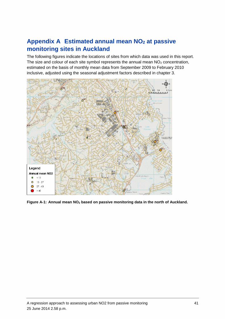
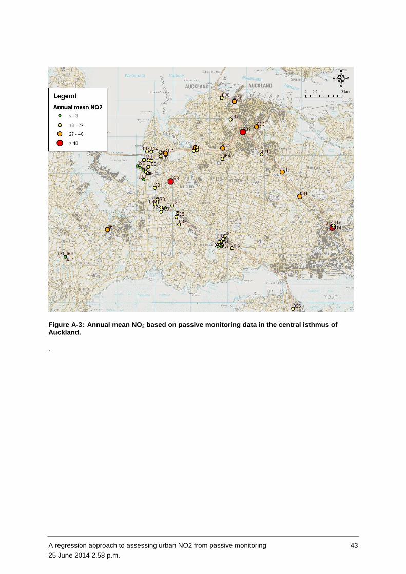
Appendix A Estimated annual mean NO2 at passive

monitoring sites in Auckland The following figures indicate the locations of sites from which data was used in this report.

The size and colour of each site symbol represents the annual mean NO2 concentration,

estimated on the basis of monthly mean data from September 2009 to February 2010

inclusive, adjusted using the seasonal adjustment factors described in chapter 3.

Figure A-1: Annual mean NO2 based on passive monitoring data in the north of Auckland.


25 June 2014 2.58 p.m.

Figure A-2: Annual mean NO2 based on passive monitoring data in the north west of Auckland.


25 June 2014 2.58 p.m.

Figure A-3: Annual mean NO2 based on passive monitoring data in the central isthmus of Auckland.

.


25 June 2014 2.58 p.m.

Figure A-4: Annual mean NO2 based on passive monitoring data in the southeast of Auckland.


25 June 2014 2.58 p.m.

Appendix B Predicted baseline NO2 at the Waterview

Connection project assessment receptors The table below lists the annual mean NO2 concentration (in g m-3) predicted by the

regression model described in this report. It should be noted that these values are lower than

those in the projects’ technical assessment report. This is because the regression model was

developed after the technical report was completed. Values in the technical report were

derived from an early trial version of the regression model and incorporated some

conservative assumptions no longer required in the current model version.

Table B-1: Annual NO2 concentrations predicted for the Waterview Project assessment receptors using the spatial regression model.

ID Receptor Name annual NO2

1 59 Victor Street Avondale College 11.7

2 12 Holly Street Avondale Intermediate 11.6

3 4 Crayford Street West Avondale Primary School 14.2

4 288 Richardson Road Christ The King School 14.4

5 8 Seaview Terrace Gladstone School 15.7

6 340 Blockhouse Bay Road Glenavon School 13.3

7 1 McLean Street Hebron Christian College 13.6

8 63 St Georges Road Immanuel Christian School 13.3

9 30-36 Alberton Avenue Mt Albert Grammar School 11.9

10 185 New Windsor Road New Windsor School 13.1

11 56 Bollard Avenue Odyssey House School Auckland 12.6

12 113-115 Richardson Road Owairaka District School 13.0

13 Moray Place Pasadena Intermediate 14.2

14 7-31 Te Ra Road Pt Chevalier School 12.0

15 217 Rosebank Road Rosebank School 11.9

16 16-20 Kotuku Street Rutherford College 15.0

17 2 Kotuku Street Rutherford School 16.1

18 2-20 Montrose Street St Francis School 22.4

19 140 Haverstock Road Te Kura Kaupapa Maori o Nga Maungarongo 12.0

20 16-20 Kotuku Street Te Kura Kaupapa Maori o Te Kotuku 13.6

21 19 Oakley Avenue Waterview School 14.9

22 776 Sandringham Road Wesley Intermediate 12.4

23 24 Potter Avenue Wesley School 11.9

24 100-102 Motions Road Western Springs College 11.3

25 24A Fairlands Avenue ABC Waterview 15.0

26 63 St Georges Road Avondale Christian Kindergarten 13.3

27 59 Victor Street Avondale College Early Childhood Centre 14.5

28 99 Rosebank Road Avondale Community Pre-School 15.9

29 195 Rosebank Road Avondale Kindergarten 15.9

30 32 Wairere Avenue Bright Beginnings ECEC Ltd. 12.4

31 28 Carrington Road Collectively Kids Limited 24.0

32 64 A Stoddard Road Edukids Stoddard Road Centre 12.4

33 830 New North Road Ferndale Kindergarten 13.6

34 340 Blockhouse Bay Road Glenavon Early Childhood Centre 17.3

35 22B Willcott Street Jump Start Kids Centre 14.7


25 June 2014 2.58 p.m.


36 2 Sandy Lane Kids World 15.6

37 4 Ennismore Road Kidz Unlimited Learning Centre 17.3

38 18 Wolverton Street Kiwicare Preschool Avondale 15.2

39 20 Wolverton Street Kiwicare Preschool West 15.2

40 25 Wolverton Street Kiwicare Wolverton 3 15.6

41 20 Huia Road Learning at the Point Kindergarten 13.5

42 14 Stewart Road Little Dudes Childcare Centre 12.0

43 6 D Carr Road Little Scholars Early Learning Centre 16.0

44 222 Carrington Road Little Scholars ELC - Mt Albert 17.2

45 122 Mt Albert Road Minimarc Childcare Centre 13.1

46 24 Mark Road Mt Albert Kindergarten 13.5

47 25 Phyllis Street Mt Albert Playcentre 15.0

48 88 Mt Royal Avenue Mt Royal Early Learning Centre 12.9

49 64 Peter Buck Road New Windsor Playcentre 11.8

50 6 A Dunkirk Terrace Owairaka Kindergarten 12.1

51 30 Walford Road Pt Chevalier Kindergarten 12.3

52 36 Blockhouse Road Rocket Kids Early Learning Centre 17.1

53 217 Rosebank Road Rosebank Early Childhood Centre 14.4

54 16-20 Kotuku Street Rutherford Preschool 15.6

55 2140 Great North Road St Marys Preschool Avondale 15.5

56 90 Point Chevalier Road Stylee Kids Ahead Early Learning Centre Limited 14.7

57 36 Titoki Street Te Puna Reo O Manawanui 21.3

58 140 Haverstock Road Te Puna Reo Maori O Nga Maungarongo 12.0

59 Gate 4 Unitec Te Puna Reo o Wairaka 17.3

60 16-20 Kotuku Street Te Kotuku Kohanga Reo 13.5

61 1217 New North Road Treasure Hunt Montessori Preschool 18.2

62 Building 57 Unitec Carrington Road Unitec Early Learning Centre 14.1

63 Carrington Road UNITEC Early Learning CentrePukeko Whare 14.1

64 10 Herdman Street Waterview Kindergarten 17.4

65 26 A O'Donnell Avenue Wesley Kindergarten 12.5

66 54 Carrington Road WDHB Addiction Unit 18.0

67 Carrington Road Mason Clinic 18.6

68 54 Carrington Road Rehab Plus 16.6

69 19 Woodward Road Aranui Hospital 14.0

70 2095 Great North Rd Avon Rest home 19.8

71 92 Rosebank Rd Avondale Rest Home & Hospital 15.6

72 39 Batkin Road Bettina Residential Care Home 12.2

73 63 Allendale Road Everill Orr Village 12.2

74 23 Roberton Road Rosaria Rest Home 17.2

75 20 Shaftsbury Avenue Selwyn Village 15.6

76 103 Tiverton Road Tiverton House Rest Home 13.9

77 45 Lloyd Ave Warrengate Private Hospital 13.2

78 46 Bollard Avenue Morwood Motorcamp 12.5

79 89 Hendon Avenue 89 Hendon Avenue 11.7

80 5 Barrymore Street 5 Barrymore Street 12.8


25 June 2014 2.58 p.m.


81 9 Valonia Street 9 Valonia Street 14.9

82 204 Methuen 204 Methuen 11.2

83 1102G Great North Road Res5 21.5

84 77 Herdman Road Res6 21.0

85 21 Alwyn Avenue 21 Alwyn Avenue 20.5

86 17 Milich Terrace Res8 20.9

87 20 Titoki Street Res9 27.2

88 7-51 Walker Road Walker Park 12.5

89 22a Phyllis Street Phyllis Reserve 15.5

90 117 Richardson Road Murray Halberg Park 11.9

91 27 Summit Drive Mt Albert-Owairaka Domain 11.9

92 2-48 Ash Street Avondale Race Course 13.3

93 63 Hendon Avenue Alan Wood Reserve 12.8

94 Denbigh Avenue Mt Roskill Intermediate 12.6

95 Frost Road Mt Roskill Grammar 13.4

96 Frost Road Mt Roskill Primary School 14.3

97 21 Currie Avenue Hillsborough Playcentre 14.1

98 1 Prospero Terrace Little Scholars Baby Cottage 14.9

99 Somerset Road Mt Roskill Early Childhood Centre 13.0

100 68 Mt Roskill Rd Gracedale Hospital 13.2

101 660 Richardson Road Keith Hay Park 12.4

Documents

Application to the Waterview Connection Prepared for … · Application to the Waterview Connection Prepared for NZ Transport ... of Water & Atmospheric Research Ltd ... mean is based