1

“An Approximate Kalman Filter forOcean Data Assimilation;

An Example with an Idealized Gulf Stream Modelt$

by

Ichim Fuku]nori

Jet Propulsion Laboratory, California Institute of Technology,4800 Oak Grove Drive, Pasadena CA 91109

and

Paola Malar~ottc-Rjzzoli

Department of Earth Atmospheric and Planetary Sciences,Massachusetts Institute of Technology,

77 Massachusetts Avenue, Cambridge MA 02139

Accepted for publication

Journal of Geophysical Research

FINAL VERSION

Nove]nber 14, 1994

2

Abstract

A practical method of data assimilation for use with large, nonlinear, ocean general

circulation models is explored. A Kalman titer based on approximations of the state

error covariance matrix is presented, e] nploying a reduction of the effective model di-

mension, the error’s asymptotic steady-state limit, and a time-invariant linearization

of the dynamic model for the error integration. The approximations lead to dramatic

computational savings in applying estimation theory to large complex systems. We ex-

amine the utility of the approximate filter in assimilating different measurement types

using a twin experiment of an idealized Gulf Stream. A nonlinear primitive equation

model of an unstable east-west jet is studied with a state dimension exceeding 170,000

elements. Assimilation of various pseudo measurements are examined, including ve-

locity, density, and volume transport at localized arrays, and realistic distributions

of satellite altimetry and acoustic tomography observations. Results are compared in

terms of their effects on the accuracies of the estimation. The approximate filter is

shown to outperform a previous study that used an empirical nudging scheme. The

examples demonstrate that useful approximate estimaticm errors can be computed in

a practical manner for general circulation models.

I3

1. Introduction

Estimating the state of the ocean circulation is one of the central issues in oceanography.

Traditionally, such studies have been pursued by two separate approaches; inductive

analyses of direct observations on the one ha] Ld and deductive studies through the

retical modeling based on first principals on tile other. A systematic approach to the

former includes inverse modeling (e.g., Martel and Wunsc.h, 1993), and the latter is rep-

resented by numerical simulations using general circulation models (e.g., Semtner and

Chervin, 1992). Most recently, the issue of conlbining the two approaches, namely data

assimilation, has received increasing attention, due primarily to the increased amount

of available obserwdions. These include both data from satellites (e.g., GEOSAT, ERS-

1, TOPEX/POSEIDON) and in situ observational experiments (e.g., WOCE, TOGA,

SYNOP). Data assimilation is a combination of data analysis and numerical modeling,

so as to make optimal use of the information content of the former and the theoretical

knowledge of the latter, which together compelwate their respective limitations. Inverse

modeling has now reached a stage that simple steady-state kinematic and geostrophic

constraints cannot fully account for all observations, but requires use of models with

more physics. On the other hand, numerical simulations suffer from inaccuracies in the

external forcing, boundary and initial conditions, and model physics including effects

of subgrid-sca.le processes.

The purpose of the present study is two-fold. The primary objective is to explore a

method that allows near-optimal but efficient assimilation with formal error estimates

using complete general circulation models. T}ke other goal is to explore assimilation of

various data types and to compare them with results obtained by nudging, which is a

simpler assimilation method. The data types considered here are direct point-wise mea-

surements of velocity, density, and volume tl ansport at localized arrays, and indirect

non-traditional measurements from satellite altimetry and acoustic tomography.

Conceptually, data assimilation modKies model variables according to what is mea-

sured and what the model physics require. Various procedures have been explored

for ocean data assimilation, which might be roughly divided into two categories. In

one, data are assimilated into comparatively complex dyx m.mical models in an ad hoc

scheme designed to “nudge” the model toward the data. Examples include nudging

(e.g., Malanotte-Rizzoli and Holland, 1986) and various forms of optimal interpolation

(e.g., Robinson et al., 1989). Another class is based on forrna.1 estimation and control

4

theory that minimizes the data-model misfit under the constraint of the model dy-

namics. These objective approaches include tl~e adjoint method (e.g., Marotzke and

Wunsch, 1993) and Kalman filtering and smoothing (e.g., I?ukumori et al., 1993).

The former class of methods lack accounti] ig for errors in the data and model, and

could conceivably introduce more errors into the model estimate than information from

the data, due to statistical and dynamic inconsistencies. The latter class, on the other

hand, involve formidable computational requirements, such that in general, applications

have been limited to simple models with less physics and/or model resolution than

typical numerical simulations. The adjoint n~ethod is generally more efficient than

Kalman filtering and smoothing, but nevertheless, involves an order of magnitude more

iterations by the forward model and its adjoint than simulations. The efficiency of the

adjoint method is attained at the expense of tile absence of formal error estimates, and

explicit error derivations would render the co] nputational cost comparable to those of

Kalman filtering and smoothing.

Thus, there is a gap between the two classes of approaches in combining data

with models. A trade-off exists between optimality with formal error estimates and

complexity of the numerical models that are used. Fukumori et al. (1993) explored

an approximate Kalman filter and smoother based on an asymptotic time-invariant

error limit, which significantly reduces the computational requirements of estimation

theory. However, their model, although a pri] aitive equation model, was still much too

simplified to be useful due primarily to the coarse resolution and to a lesser extent the

linearized dynamics. What follows is in part an extension of the work by Fukurnori

et al. (1993) in applying Kalman filtering to a model with a much finer resolution,

and thus larger state d]mension, and to one that also includes nonlinear dynamics.

Approximations will be introduced that reduce the filter’s effective dimension and sim-

plify the state’s error integration. It should be emphasized that the objective of these

simplifications is to derive an appmzirrude filter for data assimilation, and is not meant

to replace or to simplify the dynamic model per se.

Perhaps the most studied obsel ving system in the context of ocean data assimi-

lation is that by satellite altimetry [e.g., Marshall, 1985; lbbinson and Leslie, 1985;

Kindle, 1986; Holland and Malanotte-R.izzoli, 1989; White et al., 1990a, b, c; Mellor

and Ezer, 1991; Fukumori et al., 1993]. The attention to altimetry studies is primarily

5

duetothe satellites’ global andcontinuous coverage and the associated

of observations that provide stringent constraints on the estimation.

large number

In contrast, traditional oceanographic datasets have received, until now, relatively

little attention in assimilation studies. Thus far, very few papers have addressed the

issue of assimilating localized oceanogI aphic n measurements and of awessing their ef-

fectiveness in constraining a dynamical model. Idealized iwsimilations of hydrographic

surveys were carried out by Malanot te-Rizzoli and Holland (1986, 1988) and Malanotte-

Rizzoli et al. (1989). Sparse expandable bathythermographs (XBT) and infrared satel-

lite imagery (IR) were used for feature models of the Gulf Stream system by Robinson

et al. (1989) and Robinson (1992) in the HaY vard Gulfcast effort. In the equatorial

ocean, XBTS were used by Moore and Anderson (1989), and tide gauge measurements

were assimilated in the studies of Miller and Cane (1989) and c]f Smedstad and O’Brien

(1991). The study of Malanotte-Rizzoli and Young (1992) addressed the specific ques-

tion; can traditional measurements taken at localized arrays of moorings be effective

when assimilated into an ocean circulation xaodel? They used a model of the Gulf

Stream focusing on process studies, specifically aimed at reconstructing the system

behavior of a jet’s meander evolution from li] nited point- wise measurements.

Assimilation of acoustic tomography meamrements has received even less attention

than other in situ measurements. Sheinbau]n (1989) conducted simulations of tomo-

graphic assimilation using a simple one-layes model. Tomography can provide unique

continuous synoptic observations of the thredimemional interior density and velocity

field, which are not directly accessible by the surface measurements from satellites nor

by traditional in situ measurements that are sparse.

One of the ultimate goals of estimation is to combine all observations into a single

coherent model of the ocean. Ln this manuscript, we will take some steps towards

this objective and explore the problem of assimilating various types of observations

discussed above into a realistic model of the ocean. One of the major issues raised

in data assimilation is how information from observations are propagated within the

model, spatially, temporally, and among different properties. This is especially an

issue with non-traditional measurements that do not prcwide direct observations of the

model’s prognostic variables, such w+ rdtimet ry and tomography. Among the advantages

of estimation theory, Kalman filtering does not distinguish between observations of

individual prognostic variables and diagnostic quantities, and it will be straightforward

6

to assimilate altimetric or tomographic measurements as is to analyze velocity or density

data.

The present study is based on the twin experiment employed in the analysis of

Malanotte-Rizzoli and Young (1992; hereafter referred to as RY92) of an idealized model

of the Gulf Stream. The motivation for RY92 was provided by the SYNoptic Ocean

Prediction (SYNOP) experiment carried out in the period 1987--1990 in the Gulf Stream

system (Fig 1). The model configuration of RY92 was idealized, with the SYNOP

arrays schematized as two identical arrays in a rectangular domain (Fig 2). The model

is of an unstable jet, based on a non-linear, three- dirnelmional, primitive equation,

general circulation model, and they used a nudging scheme for the assimilation. We will

revisit the question of the effectiveness of localized datasets in constraining a dynamical

model with the approximate Kalman filter using this same numerical model as RY92.

One of the objectives of the present analysis is to zwsess the efficacy of a suboptimal

Kalman filter versus nudging when performing identical assimilation experiments. This

is an ambitious application of estimation theory, involving issues of the model’s large

dimension, nonlinearity, instabilities, and of the complex algorithm of the model itself.

This paper is organized as follows. In section 2.1 we briefly review some of the

issues of Kalman filtering, and introduce the reduced-order, static, linearized filter in

section 2.2. In section 3, we discuss results fron 1 the assimilation experiments. Sections

3.1 and 3.2 are devoted to describing the strategies tb.at were taken in constructing the

approximate Kalman filter for the particular example; 3.1 discusses the coarse state

approximation and linearization and 3.2 describes the choice for the data error and

model process noise used in deriving the filter. In section 3.3 we revisit the assimilation

of localized cluster data.sets examined by RY92 but using the approximate Kalman

filter, while the examples of assimilating the less traditional measurements (altimetry

and tomography) are discussed in section 3,4. In section 4, Summary and Discussion,

we present our conclusions and describe directions for future research.

2. Approximate Kalman Filter

In this section we describe a method of data assimilation based on an approximate form

of the Kalman filter. The approximation is a linearized Kalman filter that combines

use of a static estimation error covariance matrix (Fukumori et al., 1993) and a method

‘i’

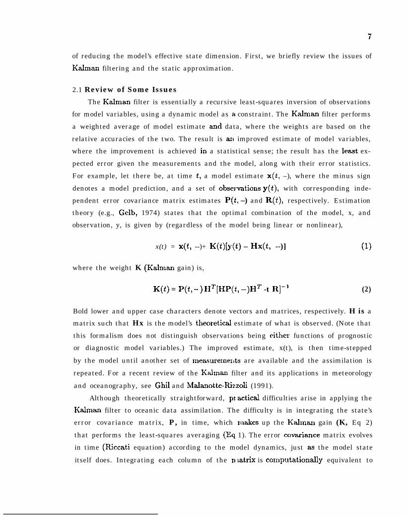
of reducing the model’s effective state dimension. First, we briefly review the issues of

Ka.lman filtering and the static approximation.

2.1 Review of Some Issues

The Kalman filter is essentially a recursive least-squares inversion of observations

for model variables, using a dynamic model as a constraint. The Kalman filter performs

a weighted average of model estimate and data, where the weights are based on the

relative accuracies of the two. The result is an improved estimate of model variables,

where the improvement is achieved in a statistical sense; the result has the least ex-

pected error given the measurements and the model, along with their error statistics.

For example, let there be, at time t, a model estimate x(t, –), where the minus sign

denotes a model prediction, and a set of obsemation.s y(t), with corresponding inde-

pendent error covariance matrix estimates P(i, –) and R(t), respectively. Estimation

theory (e.g., Gelb, 1974) states that the optimal combination of the model, x, and

observation, y, is given by (regardless of the model being linear or nonlinear),

x(t) = x(t, --)+ K(t)[y(i) – Hx(t, --)] (1)

where the weight K (Kalman gain) is,

K(t) = P(i, –) HT[HP(t, –)HT -t R]-l (2)

Bold lower and upper case characters denote vectors and matrices, respectively. H is a

matrix such that Hx is the model’s thecmeticaJ estimate of what is observed. (Note that

this formalism does not distinguish observations being either functions of prognostic

or diagnostic model variables.) The improved estimate, x(t), is then time-stepped

by the model until another set of measureme]]ts are available and the assimilation is

repeated. For a recent review of the Kalman filter and its applications in meteorology

and oceanography, see GhIl and Malanotte-Rizzoli (1991).

Although theoretically straightforward, pI actical difficulties arise in applying the

Kalrnan filter to oceanic data assimilation. The difficulty is in integrating the state’s

error covariance matrix, P, in time, which lnakes up the Kalman gain (K, Eq 2)

that performs the least-squares averaging (Eq 1). The error covariance matrix evolves

in time (Riccati equation) according to the model dynamics, just as the model state

itself does. Integrating each column of the IJ latrix is computationally equivalent to

8

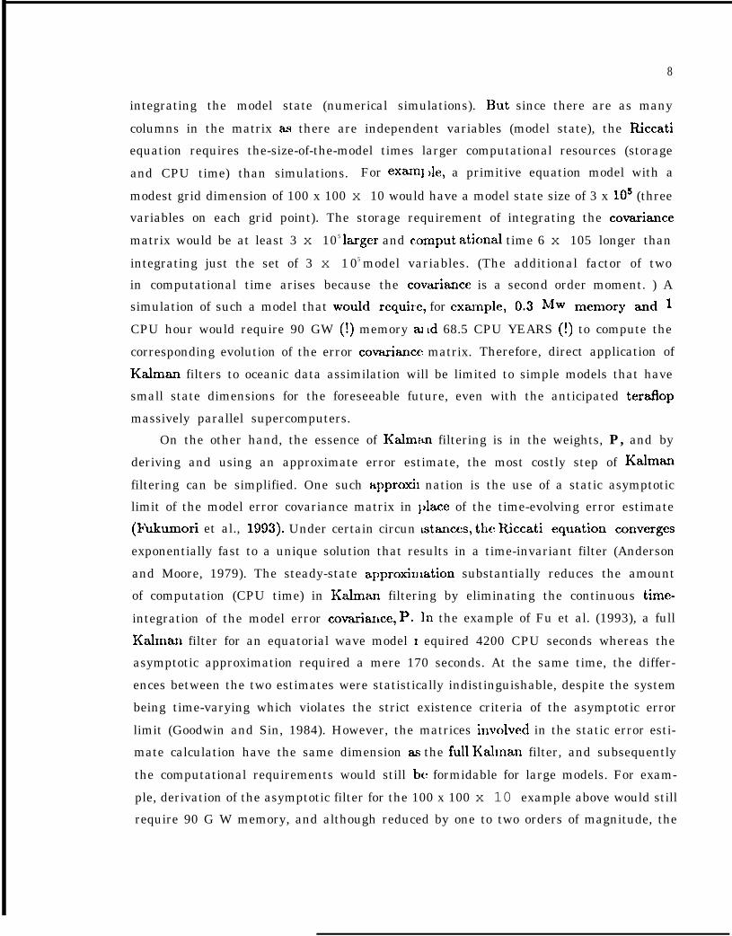
integrating the model state (numerical simulations). 13ut since there are as many

columns in the matrix as there are independent variables (model state), the Riccati

equation requires the-size-of-the-model times larger computational resources (storage

and CPU time) than simulations. For exam] de, a primitive equation model with a

modest grid dimension of 100 x 100 x 10 would have a model state size of 3 x 105 (three

variables on each grid point). The storage requirement of integrating the covariance

matrix would be at least 3 x 105 larger and c.omput ational time 6 x 105 longer than

integrating just the set of 3 x 105 model variables. (The additional factor of two

in computational time arises because the covariance is a second order moment. ) A

simulation of such a model that would require, for ex~npk 0.3 MW memory and 1

CPU hour would require 90 GW (!) memory aI id 68.5 CPU YEARS (!) to compute the

corresponding evolution of the error covariance matrix. Therefore, direct application of

Kalman filters to oceanic data assimilation will be limited to simple models that have

small state dimensions for the foreseeable future, even with the anticipated terafiop

massively parallel supercomputers.

On the other hand, the essence of Kalman filtering is in the weights, P, and by

deriving and using an approximate error estimate, the most costly step of Kalrnan

filtering can be simplified. One such approxi] nation is the use of a static asymptotic

limit of the model error covariance matrix in ]dace of the time-evolving error estimate

(Fukumori et al., 1993). Under certain circun Lsta.nces, the Rccati equation converges

exponentially fast to a unique solution that results in a time-invariant filter (Anderson

and Moore, 1979). The steady-state approxinlation substantially reduces the amount

of computation (CPU time) in Kalman filtering by eliminating the continuous time-

integration of the model error covariance, P. In the example of Fu et al. (1993), a full

Kalman filter for an equatorial wave model x equired 4200 CPU seconds whereas the

asymptotic approximation required a mere 170 seconds. At the same time, the differ-

ences between the two estimates were statistically indistinguishable, despite the system

being time-varying which violates the strict existence criteria of the asymptotic error

limit (Goodwin and Sin, 1984). However, the matrices i]wcdved in the static error esti-

mate calculation have the same dimension as the full Kahnan filter, and subsequently

the computational requirements would still bc formidable for large models. For exam-

ple, derivation of the asymptotic filter for the 100 x 100 x 10 example above would still

require 90 G W memory, and although reduced by one to two orders of magnitude, the

9

CPU time requirement would remain enormous (= 6 CPIJ months as opposed to 68.5

CPU years). Therefore, the steady-state appx oximation zdone will not make Kalman

filtering feasible for the general oceanic problem.

In the next section, we describe another a] ]proxknation which reduces the effective

dimension of the matrices involved, and with it, the storage and computational require-

ments of Kalman filtering. We emphasize agahl that the objective of the simplifications

is solely to compute an approximate model error covaria.nce matrix P and replace that

in Eqs (1, 2) for data assimilation, and is not to replace the numerical model itself.

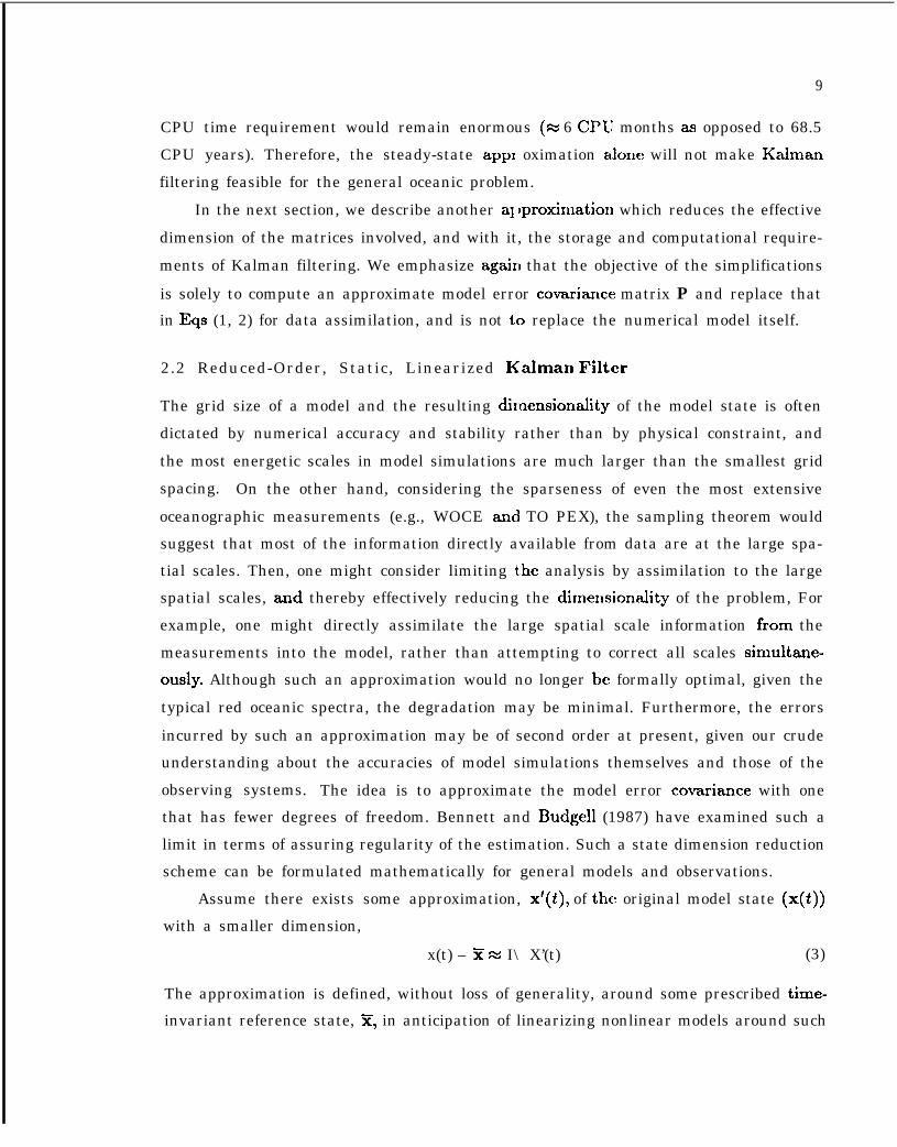
2.2 Reduced-Order, Static, Linearized Kalman Filter

The grid size of a model and the resulting dhnensionality of the model state is often

dictated by numerical accuracy and stability rather than by physical constraint, and

the most energetic scales in model simulations are much larger than the smallest grid

spacing. On the other hand, considering the sparseness of even the most extensive

oceanographic measurements (e.g., WOCE and TO PEX), the sampling theorem would

suggest that most of the information directly available from data are at the large spa-

tial scales. Then, one might consider limiting the analysis by assimilation to the large

spatial scales, and thereby effectively reducing the dimensionality of the problem, For

example, one might directly assimilate the large spatial scale information horn the

measurements into the model, rather than attempting to correct all scales simuhne-

ously. Although such an approximation would no longer be formally optimal, given the

typical red oceanic spectra, the degradation may be minimal. Furthermore, the errors

incurred by such an approximation may be of second order at present, given our crude

understanding about the accuracies of model simulations themselves and those of the

observing systems. The idea is to approximate the model error covariance with one

that has fewer degrees of freedom. Bennett and Budgell (1987) have examined such a

limit in terms of assuring regularity of the estimation. Such a state dimension reduction

scheme can be formulated mathematically for general models and observations.

Assume there exists some approximation, x’(t), of the original model state (x(t))

with a smaller dimension,

x(t) – Y N I\ X’(t) (3)

The approximation is defined, without loss of generality, around some prescribed time-

invariant reference state, Z, in anticipation of linearizing nonlinear models around such

10

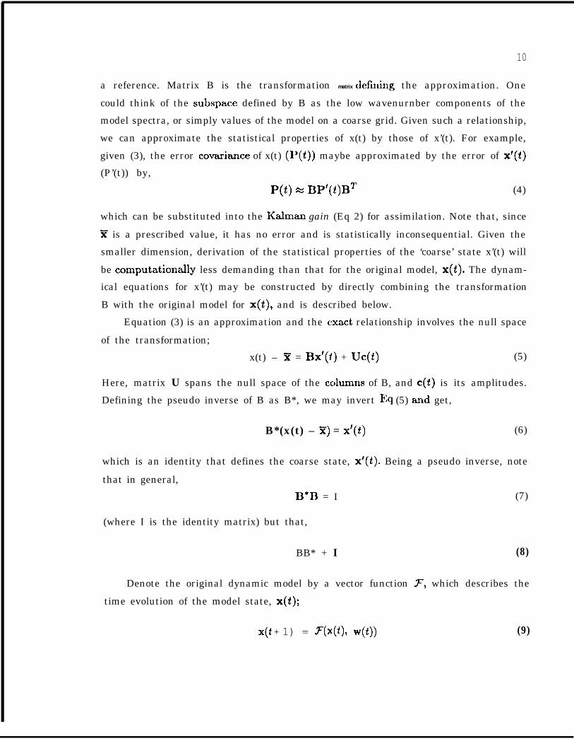
a reference. Matrix B is the transformation matrix defhling the approximation. One

could think of the subspace defined by B as the low wavenurnber components of the

model spectra, or simply values of the model on a coarse grid. Given such a relationship,

we can approximate the statistical properties of x(t) by those of x’(t). For example,

given (3), the error covariance of x(t) (P(t)) maybe approximated by the error of x’(t)

(P’(t)) by,

P(t) s BP’(i)B~ (4)

which can be substituted into the Kalrnan gain (Eq 2) for assimilation. Note that, since

x is a prescribed value, it has no error and is statistically inconsequential. Given the

smaller dimension, derivation of the statistical properties of the ‘coarse’ state x’(t) will

be computationally less demanding than that for the original model, x(t). The dynam-

ical equations for x’(t) may be constructed by directly combining the transformation

B with the original model for x(t), and is described below.

Equation (3) is an approximation and the exact relationship involves the null space

of the transformation;

x(t) – X = Bx’(t) + Uc(t) (5)

Here, matrix U spans the null space of the ccJumns of B, and c(t) is its amplitudes.

Defining the pseudo inverse of B as B*, we may invert Fq (5) and get,

B*(x(t) – Y) = X’(t) (6)

which is an identity that defines the coarse state, x’(t). Being a pseudo inverse, note

that in general,

B*B = I (7)

(where I is the identity matrix) but that,

BB* + I (8)

Denote the original dynamic model by a vector function 7, which describes the

time evolution of the model state, x(t);

X(t + 1) = f-(x(~), w(~)) (9)

—

11

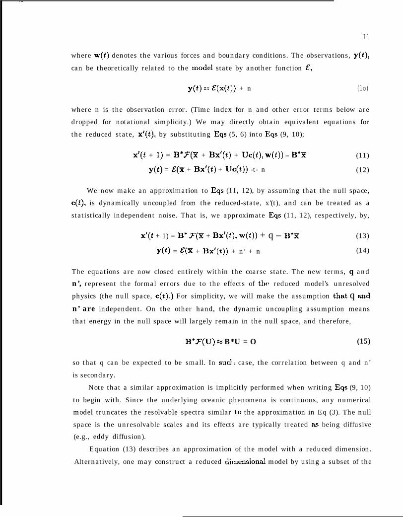
where w(t) denotes the various forces and boundary conditions. The observations, y(t),

can be theoretically related to the model state by another function &,

y(t) == &(x(t)) + n (lo)

where n is the observation error. (Time index for n and other error terms below are

dropped for notational simplicity.) We may directly obtain equivalent equations for

the reduced state, x’(t), by substituting Eqs (5, 6) into Fkqs (9, 10);

x’(t + 1) = B*7(z + Bx’(t) + Uc(t), w(t)) – B*Y (11)

y(t) = S(% + Bx’(t) + IJc(t)) -t- n (12)

We now make an approximation to Eqs (11, 12), by assuming that the null space,

c(t), is dynamically uncoupled from the reduced-state, x’(t), and can be treated as a

statistically independent noise. That is, we approximate Eqs (11, 12), respectively, by,

x’(t + 1) = B* X(= + Bx’(t), w(~)) + q – B*Y (13)

(14)y(~) = F(X + 13x’(t)) + n’ + n

The equations are now closed entirely within the coarse state. The new terms, q and

n’, represent the formal errors due to the effects of the reduced model’s unresolved

physics (the null space, c(t).) For simplicity, we will make the assumption that q andn’ are independent. On the other hand, the dynamic uncoupling assumption means

that energy in the null space will largely remain in the null space, and therefore,

so that q can be expected to be

is secondary.

B*3(U) N B*U = O (15)

small. In SUCI 1 case, the correlation between q and n’

Note that a similar approximation is implicitly performed when writing Eqs (9, 10)

to begin with. Since the underlying oceanic phenomena is continuous, any numerical

model truncates the resolvable spectra similar to the approximation in Eq (3). The null

space is the unresolvable scales and its effects are typically treated as being diffusive

(e.g., eddy diffusion).

Equation (13) describes an approximation of the model with a reduced dimension.

Alternatively, one may construct a reduced dhnensional model by using a subset of the

12

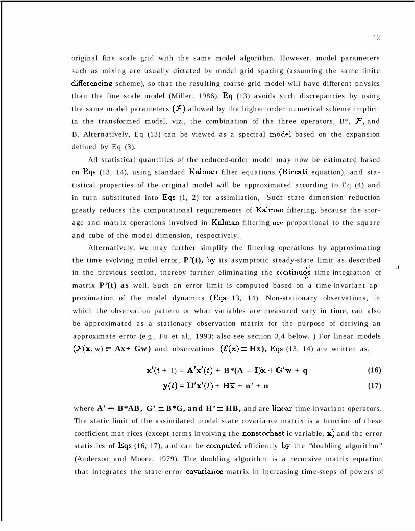
original fine scale grid with the same model algorithm. However, model parameters

such as mixing are usually dictated by model grid spacing (assuming the same finite

differencing scheme), so that the resulting coarse grid model will have different physics

than the fine scale model (Miller, 1986). Eq (13) avoids such discrepancies by using

the same model parameters (>) allowed by the higher order numerical scheme implicit

in the transformed model, viz., the combination of the three operators, B*, ~, and

B. Alternatively, Eq (13) can be viewed as a spectral rnoclel based on the expansion

defined by Eq (3).

All statistical quantities of the reduced-order model may now be estimated based

on Eqs (13, 14), using standard Kalman filter equations (Riccati equation), and sta-

tistical properties of the original model will be approximated according to Eq (4) and

in turn substituted into Eqs (1, 2) for assimilation, Such state dimension reduction

greatly reduces the computational requirements of Kalman filtering, because the stor-

age and matrix operations involved in Kalman filtering arc proportional to the square

and cube of the model dimension, respectively.

Alternatively, we may further simplify the filtering operations by approximating

the time evolving model error, P’(t), by its asymptotic steady-state limit as described

in the previous section, thereby further eliminating the ccmtinu~$ time-integration of -\

matrix P’(t) as well. Such an error limit is computed based on a time-invariant ap-

proximation of the model dynamics (Eqs 13, 14). Non-stationary observations, in

which the observation pattern or what variables are measured vary in time, can also

be approximated as a stationary observation matrix for the purpose of deriving an

approximate error (e.g., Fu et al,, 1993; also see section 3,4 below. ) For linear models

(7(x, w) - Ax+ Gw) and observations ($(x) s Hx), Eqs (13, 14) are written as,

x’(t + 1) = A’x’(t) + B*(A – I)Y+ G’w + q (16)

y(t) = H’x’(t) + H% + n’ + n (17)

where A’ s B*AB, G’ s B*G, and H’ a HB, and are linear time-invariant operators.

The static limit of the assimilated model state covariance matrix is a function of these

coefficient mat rices (except terms involving the nonstochast ic variable, X) and the error

statistics of Eqs (16, 17), and can be computecl efficiently by the “doubling algorithm”

(Anderson and Moore, 1979). The doubling algorithm is a recursive matrix equation

that integrates the state error cova,riance matrix in increasing time-steps of powers of

13

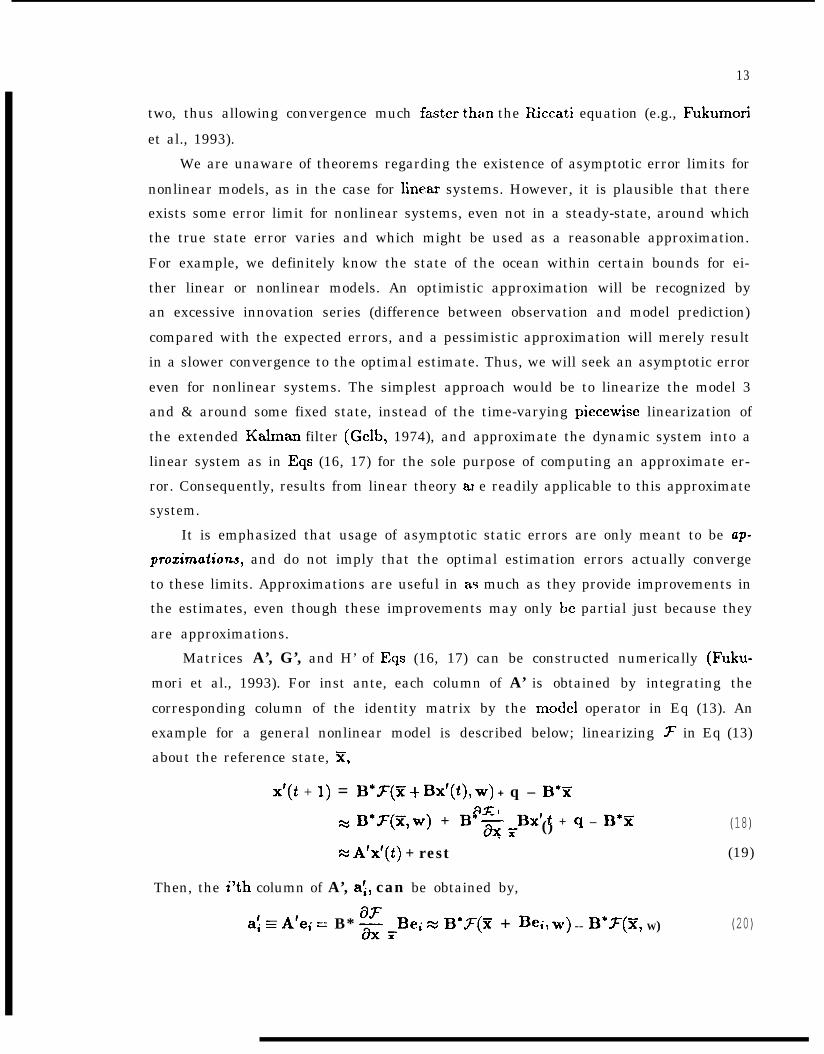
two, thus allowing convergence much faster than the Riccati equation (e.g., Fukumori

et al., 1993).

We are unaware of theorems regarding the existence of asymptotic error limits for

nonlinear models, as in the case for linear systems. However, it is plausible that there

exists some error limit for nonlinear systems, even not in a steady-state, around which

the true state error varies and which might be used as a reasonable approximation.

For example, we definitely know the state of the ocean within certain bounds for ei-

ther linear or nonlinear models. An optimistic approximation will be recognized by

an excessive innovation series (difference between observation and model prediction)

compared with the expected errors, and a pessimistic approximation will merely result

in a slower convergence to the optimal estimate. Thus, we will seek an asymptotic error

even for nonlinear systems. The simplest approach would be to linearize the model 3

and & around some fixed state, instead of the time-varying piecewise linearization of

the extended Kalman filter (Gelb, 1974), and approximate the dynamic system into a

linear system as in Eqs (16, 17) for the sole purpose of computing an approximate er-

ror. Consequently, results from linear theory aI e readily applicable to this approximate

system.

It is emphasized that usage of asymptotic static errors are only meant to be up-

prozimatiow, and do not imply that the optimal estimation errors actually converge

to these limits. Approximations are useful in a.~ much as they provide improvements in

the estimates, even though these improvements may only be partial just because they

are approximations.

Matrices A’, G’, and H’ of Eqs (16, 17) can be constructed numerically (Fuku-

mori et al., 1993). For inst ante, each column of A’ is obtained by integrating the

corresponding column of the identity matrix by the moclel operator in Eq (13). An

example for a general nonlinear model is described below; linearizing F in Eq (13)

about the reference state, Y,

x’(t + 1) = B“>(5E+ Bx’(t), w) + q – B*xW

I ()N B*~(~,w) + B*X =BX’ t + q – B*Z (18)

N A’x’(i) + rest (19)

Then, the i’th column of A’, a\, can be obtained by,

a: = A’ei == B* ~ ~Bei x B*F(X + Ihi, w) -- B*.F(~, W) (20)

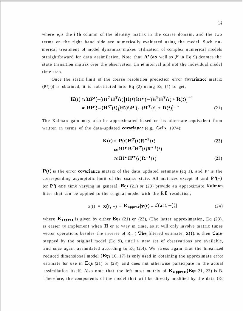
14

where ei is the i’th column of the identity matrix in the coarse domain, and the two

terms on the right hand side are numerically evaluated using the model. Such nu-

merical treatment of model dynamics makes utilization of complex numerical models

straightforward for data assimilation. Note that A’ (as well as ~ in Eq 9) denotes the

state transition matrix over the observation tin ie interval and not the individual model

time step.

Once the static limit of the coarse resolution prediction error covariance matrix

(P’(–)) is obtained, it is substituted into Eq (2) using Eq (4) to get,

K(t)s BP’(–) BTHT(t) [H(t) BIJ’(-)BTH7’(t) + R(t)]’1

= BP’(–)H’T(i) [H’(i)P’(- )H’T(i) + R(i)] ‘1 (21)

The Kalman gain may also be approximated based on its alternate equivalent form

written in terms of the data-updated covariance (e.g., Gelb, 1974);

K(i) = P@)HT(i)R-l (t) (22)

N BIJ’BTHT’(i)R- 1 (i)

R BP’H’T(i)R-l (i) (23)

P(t) is the error covariance matrix of the data updated estimate (eq 1), and P’ is the

corresponding asymptotic limit of the coarse state. All matrices except B and P’(–)

(or P’) are time varying in general. Eqs (21) or (23) provide an approximate Kahnan

filter that can be applied to the original model with the full resolution;

x(t) = x(t, –) + KtapprOZ[Y(~) – ~(x(ft –))1 (24)

where KoPPrOz is given by either Eqs (21) or (23), (The latter approximation, Eq (23),

is easier to implement when H or R vary in time, as it will only involve matrix times

vector operations besides the inverse of R,. ) ~’he filtered estimate, x(t), is then time-

stepped by the original model (Eq 9), until a new set of observations are available,

and once again assimilated according to Eq (2.4). We stress again that the linearized

reduced dimensional model (Eqs 16, 17) is only used in obtaining the approximate error

estimate for use in Eqs (21) or (23), and does not otherwise participate in the actual

assimilation itself, Also note that the left most matrix of K@ PPrOz (Eqs 21, 23) is B.

Therefore, the components of the model that will be directly modified by the data (Eq

15

24) is limited to the range space of B. For example, if B is an interpolation operator

that transforms the large spatial scales onto the fine grid, the short scales present in

the model prediction, x(t, –), are unmodified by Eq (24). However, smaller scales

will subsequently be generated and modified by the model itself (%) in the prediction

phase of Kalman filtering; i.e., in computing x(t + 1, –) from x(t) by the original full

resolution nonlinear model, Eq (9).

3. Assimilation Experiments

We now examine the utility of the approximations described in the preceding sections,

in an identical twin experiment. A twin experiment is a simulation of data assimilation.

Two model simulations are run starting from two indepenckmt initial conditions, from

one simulation pseudo observations are taken and assimilated into the other, to see

how well the state of the former can be estimated. The degree of how much the former

state is recovered provides a measure of the observation’s information content and the

skill of the assimilation scheme.

The twin experiment ex~ned in. this study is the idealized Gulf Stream model

of RY92 (Malanotte-Rizzoli and Young, 1992), whose motivation was provided by the

SYNoptic Ocean Prediction (SYNOP) experiment carried cmt in the period 1987-1990

in the Gulf Stream system. The scientific objective of SYNOP was to understand the

structure and variability of the system and to prdlct the evolution of the Stream den-

sity front. SYNOP consisted of three major arrays of moorings, the Inlet array, located

at Cape Hatteras, where the Stream leaves the coast and meanders into the ocean inte-

rior; the Central array, located at N 68”W, west of the New England Seamounts; and

the Eastern array, located at N 55°W. Figure 1 shows the actual field work configura-

tion of SYNOP. The focus of RY92 was to examine whether constraints provided by

localized arrays are strong enough for the model dynamics to reconstruct Gulf Stream

processes, and was considered in an idealized nlodel of the SYNOP experiment.

In the study of RY92, the Central and Eastern arrays were schematized as two

identical arrays of moorings in an idealized zonal channel with an unstable east-west

jet (Fig 2). The model is based on the Semispectral Primitive Equation Model (SPEM;

Haidvogel et al., 1991), with a fixed inflow at the western boundary. The eastern

end has a dynamic open boundary condition (Orlanski, 1976), whereas the northern

and southern boundary conditions are free- sli~), no-normal flow. The model uses the

16

rigid-lid approximation, and has advective nordinearities in momentum and density.

The model domain is 1875 km zonally, and 1400 km meridionally with a flat bottom

at a constant depth of 4000 m. The total model grid is 129 x 97 horizontally with 5

collocation points in the vertical. The horizolltd resolution is approximately 14 km,

and a 20 minute model time stepping is used.

A control experiment is carried out by running a simulation for 300 days starting

horn an analytically prescribed form of a geostrophically and hydrostatically balanced,

zonally uniform jet. The model is unstable, with meanders growing into large amplit-

udes, and pinching off eddies. The twin experiment is carried out as described in Fig

3, Pseudo measurements are taken at two day intervals between days 60 to 120 of the

simulation, and are assimilated into the model, initialized to day 180 of the control run.

For convenience, the first simulation from which pseudo data are obtained is referred to

as the “true ocean” (days 60 to 120 of the control run), while the second simulation is

the “false ocean” (days 180 to 240 of the control run). The assimilated estimate is the

“model ocean” (initialized by day 180 of the control, but modified by the assimilation).

The decorrelation time of the control run was approxirnatel.y 12 days, and therefore the

60-day time separation between the “true ocean” and the “false ocean” can be regarded

as statistically uncorrelated. Figure 4 shows an example of the evolution of the surface

density anomaly in the “true ocean” (left panels) and the “false ocean” (right panels).!’

The assimilated measurements of RY92 included~ current velocities, densities (tern- )~

peratures), and transport stream functions (volume trmlsports) at the two arrays of

thirteen moorings (Fig 2) with measurements taken on each of the five depths at each

location. Using a simple time-continuous nudging scheme, with the tw~day pseudo

data linearly interpolated in time, RY92 found that velocity measurements were effec-

tive in recovering the “true ocean”, where an event of meander formation, steepening,

bending, and breaking off was resolvecl (denoted A through E in Fig 4). The mean-

der event was localized in the region roughly between the two arrays, almost void of

measurements. However, there was little improvement with density assimilation, and

nudging stream function resulted in making the errors increase over the “false ocean. ”

The simple “nudging” scheme used in RY92 involves appending to the model prog-

nostic equations a forcing term that relaxes the model vm-iables to the observations.

The nudging factor, an inverse time scale, is a measurement of the weight given to the

data versus the model predicted variables. Even though the nudging scheme proved

to be very successful, it is still a very crude assimilation. method.

constrains the model only locrdly near the actual data points. It is

17

The information

left to the model

dynamics to perform the advection of information fro]m the data-dense to the data-void

regions and from one measured prognostic variable to the unmeasured variables.

We will now revisit the questions raised by RY92 using the approximate Kalman

filter, which is capable of spreading the localized information throughout the model

domain and different variables in an optimal fashion. Additionally, assimilation of

other types of observations will also be examined as to how well they constrain the

estimation, including sea level from satellite altimetry and integrated measurements of

acoustic tomography.

Sections 3.1 and 3.2 describe details of deriving the approximate filter presented

in section 2 for this particular experiment, and readers interested in the results of

the calculation may directly proceed to section 3.3 at first reading, without loss of

continuity.

3.1 Coarse State Approximation and Linearization

The premise of the reduced state dimension approximation is two-fold; i) that the

coarse state approximates the model’s true state (Eq 3), ii) that the null space of the

transformation, B, is approximately uncoupled from the range space dynamically (Eq

13). The selection of B will be described with regard to these requirements. The SPEM

model is a primitive equation model, with the hydrostatic and rigid lid approximations,

and the state vector consists of the two components of horizontal velocity and density

on the three-dimensional grid. All other variables, such as vertical velocity and sea

surface pressure, are computed diagnostically from these prognostic variables. The

values along the open boundary are dynamically updatecl, and as such are also part

of the state vector. The total state dimension without the coarse approximation is

172,252. As the model will later be linearized around the time-mean structure, the

coarse state will be defined as variability around this mean (%), which is shown in Fig

5.

Based on requirement ii) above, the natural reducticm in the vertical would be an

expansion into linear dynamic modes, with their arnplitu des constituting the elements

of the state vector. Vertical expansion into dynamical mc)des show that the barotropic

and first baroclinic modes together account for 9970 of the total velocity variability and

76% for density. The lesser skill in density is due tc) the nonlinear nature of the model

18

jet; the baroclinic modes of density have zero amplitude at the surface and bottom,

but the model’s density variations are due to the strong advective nonlinearities, which

require higher modes to resolve. However, inclusion of higher order density modes will

necessitate the corresponding velocity modes to be included as well, and so were not

made part of the approximation. On the othe] hand, the two horizontzd components

of the barotropic velocity are dependent due to the rigid-lid approximation and satisfy

non-divergence. Therefore stream function or ba.rotropic vorticity can replace velocity’s

two barotropic components, further reducing the state dimension. The present study

will utilize the latter in the coarse state approximation.

There are no readily available dynamic modes in the horizontal dimension for the

present study, so an alternative approach is taken. The spatial scale and structure of

the dominant variability can be assessed by examining the structures of the empirical

orthogonal functions (EOFS). Let Z denote a matrix whose columns are the leading n

EOFS of a vector, z. Then, z may be approxin Lated M,

where b is a vector consisting of the

zxZb (25)

EOFS’ expansion coefficients, and is given by,

b = iitTz (26)

Then,

z = ZZ1’Z (27)

and the matrix ZZT is the resolution matrix, as in linear inverse theory, which de-

scribes the linear combinations of the elements of z that are resolved by the n EOFS.

Alternatively, the rows of ZZT characterize the correlation among the elements of z

that dominate z’s variability.

Fig 6 shows results of an EOF analysis of the meridional variations of the two

velocity components and density, around the time-mean structure of the jet. It is

found that from among the 96 degrees of freedom (95 for meridional velocity), 13 modes

will account for at least 97910 of the variability y for all three variables. The resolution

matrix constructed by these thirteen modes is shown in Fig 7 for zonal velocity. The

matrix is diagonally dominant, with its width narrowest about the axis of the jet and

increasing towa,rds the north and south boundaries. Based on this analysis, a coarse

19

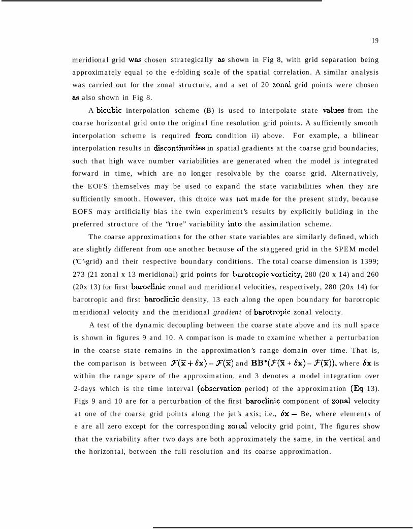
meridional grid was chosen

approximately equal to the

strategically as shown in Fig 8, with grid separation being

e-folding scale of the spatial correlation. A similar analysis

was carried out for the zonal structure, and a set of 20 zonal grid points were chosen

as also shown in Fig 8.

A bicubic interpolation scheme (B) is used to interpolate state values from the

coarse horizontal grid onto the original fine resolution grid points. A sufficiently smooth

interpolation scheme is required horn condition ii) above. For example, a bilinear

interpolation results in discontinuities in spatial gradients at the coarse grid boundaries,

such that high wave number variabilities are generated when the model is integrated

forward in time, which are no longer resolvable by the coarse grid. Alternatively,

the EOFS themselves may be used to expand the state variabilities when they are

sufficiently smooth. However, this choice was lLOt made for the present study, because

EOFS may artificially bias the twin experiment’s results by explicitly building in the

preferred structure of the “true” variability into the assimilation scheme.

The coarse approximations for the other state variables are similarly defined, which

are slightly different from one another because c~f the staggered grid in the SPEM model

(’C’-grid) and their respective boundary conditions. The total coarse dimension is 1399;

273 (21 zonal x 13 meridional) grid points for barotropic vorticity, 280 (20 x 14) and 260

(20x 13) for first baroclinic zonal and meridional velocities, respectively, 280 (20x 14) for

barotropic and first baroclinic density, 13 each along the open boundary for barotropic

meridional velocity and the meridional gradient of barotropic zonal velocity.

A test of the dynamic decoupling between the coarse state above and its null space

is shown in figures 9 and 10. A comparison is made to examine whether a perturbation

in the coarse state remains in the approximation’s range domain over time. That is,

the comparison is between 7(x+ 6x) -- Z(X) and BB*(.F(X + Jx) – .F(Y)), where 6X is

within the range space of the approximation, and 3 denotes a model integration over

2-days which is the time interval (c)bservation period) of the approximation (Eq 13).

Figs 9 and 10 are for a perturbation of the first baroclinic component of zonal velocity

at one of the coarse grid points along the jet’s axis; i.e., 6X == Be, where elements of

e are all zero except for the corresponding ZO1 lal velocity grid point, The figures show

that the variability after two days are both approximately the same, in the vertical and

the horizontal, between the full resolution and its coarse approximation.

20

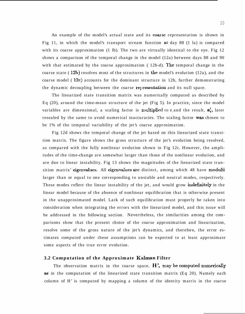
An example of the model’s actual state and its coarse representation is shown in

Fig 11, in which the model’s transport stream function at day 88 (1 la) is compared

with its coarse approximation (1 lb). The two are virtually identical to the eye. Fig 12

shows a comparison of the temporal change in the model (12a) between days 88 and 90

with that estimated by the coarse approximation ( 12b-d). I“’he temporal change in the

coarse state ( 12b) resolves most of the structures in the model’s evolution (12a), and the

coarse model ( 12c) accounts for the dominant structure in 12b, further demonstrating

the dynamic decoupling between the coarse re~lresentation and its null space.

The linearized state transition matrix was numerically computed as described by

Eq (20), around the time-mean structure of the jet (Fig 5). In practice, since the model

variables are dimensional, a scaling factor is nndtiplied to ei and the result, a{, later

resealed by the same to avoid numerical inaccuracies. The scaling factor was chosen to

be 1% of the temporal variability of the jet’s coarse approximation.

Fig 12d shows the temporal change of the jet based on this linearized state transi-

tion matrix. The figure shows the gross structure of the jet’s evolution being resolved,

as compared with the fully nonlinear evolution shown in Fig 12c. However, the ampli-

tudes of the time-change are somewhat larger than those of the nonlinear evolution, and

are due to linear instability. Fig 13 shows the magnitudes of the linearized state tran-

sition matrix’ eigenvalues. All eigenvzdues tie distinct, among which 48 have moddli

larger than or equal to one corresponding to unstable and neutral modes, respectively.

These modes reflect the linear instability of the jet, and would grow indefiltely in the

linear model because of the absence of nonlinear equilibration that is otherwise present

in the unapproximated model. Lack of such equilibration must properly be taken into

consideration when integrating the errors with the linearized model, and this issue will

be addressed in the following section. Nevertheless, the similarities among the com-

parisons show that the present choice of the coarse approximation and linearization,

resolve some of the gross nature of the jet’s dynamics, and therefore, the error es-

timates computed under these assumptions can be expected to at least approximate

some aspects of the true error evolution.

3.2 Computation of the Approximate Kalman Filter

The observation matrix in the coarse space, H’, my be computed n~ericallyas in the computation of the linearized state transition matrix (Eq 20). Namely each

column of H’ is computed by mapping a column of the identity matrix in the coarse

21

domain into the fine resolution, from which tile observed quantity is computed as in

the forward model computation. The observation matrix is rather trivial when the

measurement is one of the state elements, but becomes complex when the observation

is a nontrivial function of the state, such as the stream function, or altimetric and

tomographic measurements discussed later in sections 3.3 and 3.4. Many algorithmic

simplifications are achieved by this numerical formulation, as is also the case with the

state transition matrix (section 2.2).

In order to formulate the Kahnan filter, one further needs an estimate of the

observation error and the model’s process noise covariance matrices, besides the tran-

sition matrix and the observation matrix. Strictly speaking, being an identical twin

experiment, the present simulation is pathological, having zero process noise and ob-

servation error (no artificial error is added to the pseudo measurements), and the only

error source is the errors associated with the initial condition. Thus, if the model is

fully observable and ignoring model nonlinearities, the estimation errors will eventually

become zero, and the “true ocean” will be fully recovered by the “model ocean”.

However, the model dimension does not allow such a computation, which is why

we resort to the present approximate filter. The approximate filter has sources of errors

due to the unresolved small scale variability, which are present in the observations but

whose interactions with the coarse state are not dynamically modeled (q, n’ in Eqs

13, 14). Such errors are estimated below, which will be validated a posteriori from the

results of the assimilation.

The observation error of the reduced dime] lsion approximation is due to the vari-

ations associated with the small scales not resolved by the coarse state transformation

(n’ in Eq 14). An estimate of such contributio]ls can be made by comparing the sim-

ulation’s variabilities and their coarse represe] dations. B/wed on such analyses, the

observation errors were treated as being white horizontally, with variance equaling the

root-mean-square difference between the fine state (Hx) ancl its coarse representation

(H(BB*(x–5t)+5F)). Vertically, the errors were modeled in terms of the SPEM model’s

Chebychev modal expansion, with each amplitude being uncorrelated with the others.

The Kalman filter assumes the observational errors (n’ -+ n in Eq 17) to be white in

time. However, the small scale variations are correlated over the two-day observation

period. For example, small eddies unresolved by the coarse approximation last much

longer than two-days. In such circumstances, the model will become overconstrained

22

by the correlated errors unless the measurements are whitened. Gelb (1974) describes

such whitening methods by differencing the measurements. In the present situation, a

simpler approximation is made in which we increase the observational errors by some

factor, /?, and thereby effectively reducing the significance of the correlated measure-

ments. Such simplifications are sensible, realizing that the present calculation is only

aiming to derive an approximate model error. Several @ values were experimented with

(as well as for ~ and a below), and the combination with the best skill with consistent

estimation errors (e.g., Fig 22) are presented below. This error increase factor, ~, was

set to 10 for the results below.

The reduced-dimension approximation’s process noise (q in Eq 13) is due to the

interactions between the coarse state and the small scale variability unresolved by the

approximation. This error source is difficult to evaluate, and as such we shall model

it simply as being a white noise in the coarse domain, with variance proportional to

the time-mean variance of the simulation’s coarse state representation. The propor-

tionality factor (~) was set equal to 0.1. On the other hand, due to the difference in

spin-up time-scale, this specification will lead to a relative overestimate of the baro-

clinic component over the btiotropic part (e.g., Fukumori et al., 1993), Furthermore,

an additional source of process noise exists for density, because the quasi-geostrophic

modes do not adequately describe the density variations as discussed in section 3.1.

Therefore, an additional factor was multiplied to ~ for each separate coarse state vari-

able. These factors, (~c, 7U, -yV, 7N, ~P1 ), for barotropic vorticit y, the two components

of first baroclinic velocity, and the baxotropic and baroclinic density, respectively, were

set to (2, 0.5, 0.5, 4, 2).

The asymptotic steady-state error is computed by the doubling algorithm (Ander-

son and Moore, 1979). Such limit can be shown to exist uniquely, if the unstable and

neutral modes of the model are both observable and stochastica.lly controllable (Good-

win and Sin, 1984). Observability is the ability to determine the state from observations

in the absence of errors, and stochastic controllability is the ability to force the model

from one arbitrary state to another by the model process noise (e.g., Gelb 1974). In

particular, a mode can be shown to be observable when the norm of its projection with

the observation matrix is nonzero (Hautus, 1969). Fig 13 clemonstrates that the model

is fully observable by the velocity observations, and since process noise was modeled

as being white, all modes are also controllable. Therefore, the asymptotic error limit

23

exists for the present linearized model. (See, for example, Fukumori et al. (1993) for

more details regarding the existence and computation of the asymptotic static filter. )

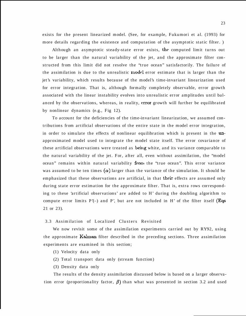
Although an asymptotic steady-state error exists, the computed limit turns out

to be larger than the natural variability of the jet, and the approximate filter con-

structed from this limit did not resolve the “true ocean” satisfactorily. The failure of

the assimilation is due to the unrealistic model error estimate that is larger than the

jet’s variability, which results because of the model’s time-invariant linearization used

for error integration. That is, although formally completely observable, error growth

associated with the linear instability evolves into unrealistic error amplitudes until bal-

anced by the observations, whereas, in reality, error growth will further be equilibrated

by nonlinear dynamics (e.g., Fig 12).

To account for the deficiencies of the time-invariant linearization, we assumed con-

tributions from artificial observations of the entire state in the model error integration,

in order to simulate the effects of nonlinear equilibration which is present in the un-

approximated model used to integrate the model state itself. The error covariance of

these artificial observations were treated as bei]lg white, and its variance comparable to

the natural variability of the jet. For, after all, even without assimilation, the “model

ocean” remains within natural variability fron~ the “true ocean”. This error variance

was assumed to be ten times (a) larger than the variance of the simulation. It should be

emphasized that these observations are artificial, in that their effects are assumed only

during state error estimation for the approximate filter. That is, extra rows correspond-

ing to these ‘artificial observations’ are added to H’ during the doubling algorithm to

compute error limits P’(–) and P’, but are not included in H’ of the filter itself (Eqs

21 or 23).

3.3 Assimilation of Localized Clusters Revisited

We now revisit some of the assimilation experiments carried out by RY92, using

the approximate Kalmrm filter described in the preceding sections. Three assimilation

experiments are examined in this section;

(1) Velocity data only

(2) Total transport data only (stream function)

(3) Density data only

The results of the density assimilation discussed below is based on a larger observa-

tion error (proportionality factor, fl) than what was presented in section 3.2 and used

24

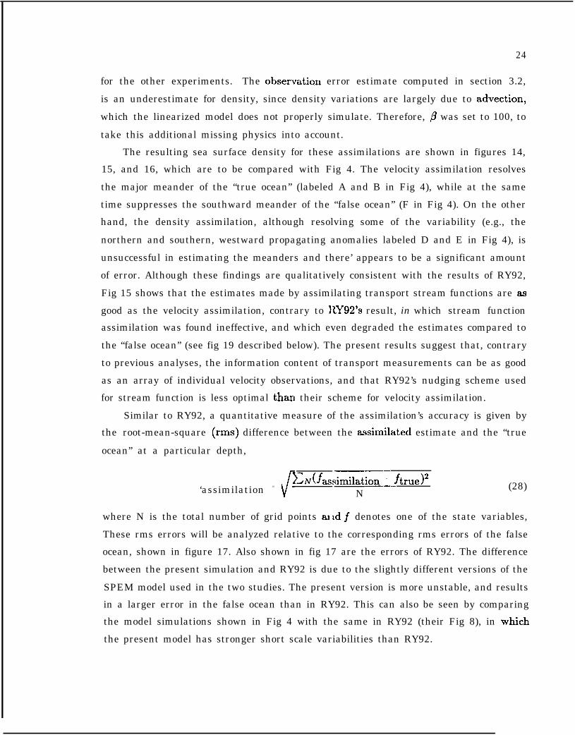
for the other experiments. The observatim error estimate computed in section 3.2,

is an underestimate for density, since density variations are largely due to advection,

which the linearized model does not properly simulate. Therefore, @ was set to 100, to

take this additional missing physics into account.

The resulting sea surface density for these assimilations are shown in figures 14,

15, and 16, which are to be compared with Fig 4. The velocity assimilation resolves

the major meander of the “true ocean” (labeled A and B in Fig 4), while at the same

time suppresses the southward meander of the “false ocean” (F in Fig 4). On the other

hand, the density assimilation, although resolving some of the variability (e.g., the

northern and southern, westward propagating anomalies labeled D and E in Fig 4), is

unsuccessful in estimating the meanders and there’ appears to be a significant amount

of error. Although these findings are qualitatively consistent with the results of RY92,

Fig 15 shows that the estimates made by assimilating transport stream functions are as

good as the velocity assimilation, contrary to RY92’s result, in which stream function

assimilation was found ineffective, and which even degraded the estimates compared to

the “false ocean” (see fig 19 described below). The present results suggest that, contrary

to previous analyses, the information content of transport measurements can be as good

as an array of individual velocity observations, and that RY92’s nudging scheme used

for stream function is less optimal than their scheme for velocity assimilation.

Similar to RY92, a quantitative measure of the assimilation’s accuracy is given by

the root-mean-square (rrns) difference between the awirnilated estimate and the “true

ocean” at a particular depth,

‘assimilation =

{

——.>;zv(.fassirnilation - ~true)2—-

N(28)

where N is the total number of grid points aI Ld ~ denotes one of the state variables,

These rms errors will be analyzed relative to the corresponding rms errors of the false

ocean, shown in figure 17. Also shown in fig 17 are the errors of RY92. The difference

between the present simulation and RY92 is due to the slightly different versions of the

SPEM model used in the two studies. The present version is more unstable, and results

in a larger error in the false ocean than in RY92. This can also be seen by comparing

the model simulations shown in Fig 4 with the same in RY92 (their Fig 8), in whkh

the present model has stronger short scale variabilities than RY92.

25

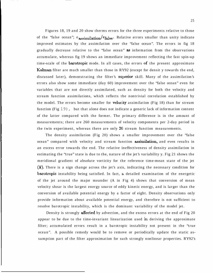
Figures 18, 19 and 20 show therms errors for the three experiments relative to those

of the “false ocean”; e~simi~ation/ef~se. Relative errors smaller than unity indicate

improved estimates by the assimilation over the “false ocean”. The errors in fig 18

gradually decrease relative to the “false ocean” as information from the observations

accumulate, whereas fig 19 shows an immediate improvement reflecting the fast spin-up

time-scale of the barotropic mode. In all cases, the errors of the present approximate

Kalman filter are much smaller than those in RY92 (except for densit y towards the end,

discussed later), demonstrating the filter’s su~jerior skill. Many of the assimilation’s

errors also show some immediate (day 60) improvement over the “false ocean” even for

variables that are not directly assimilated, such as density for both the velocity and

stream function assimilations, which reflects the nontrivial correlation established by

the model. The errors become smaller for velQcity assimilation (Fig 18) than for stream

function (Fig 19), but that alone does not indicate a generic lack of information content

of the latter compared with the former. The primary difference is in the amount of

measurements; there are 260 measurements of velocity components per 2-day period in

the twin experiment, whereas there are only 26 stream function measurements.

The density assimilation (Fig 20) shows a smaller improvement over the “false

ocean” compared with velocity and stream function assix~ilation, and even results in

an excess error towards the end. The relative ineffectiveness of density assimilation in

estimating the “true” state is due to the, nature of the jet’s variability y. Fig 21 shows the

meridional gradient of absolute vorticity for the reference time-mean state of the jet

(z). There is a sign change across the jet’s axis, indicating the necessary condition for

barotropic instability being satisfied. In fact, a detailed examination of the energetic

of the jet around the major meander (A in Fig 4) shows that conversion of mean

velocity shear is the largest energy source of eddy kinetic energy, and is larger than the

conversion of available potential energy by a factor of eight. Density observations only

provide information about available potential energy, and therefore is not sufficient to

resolve barotropic instability, which is the dominant variability of the model jet.

Density is strongly aflected by advection, and the excess errors at the end of Fig 20

appear to be due to the time-invariant linearization used in deriving the approximate

filter; accumulated errors result in a barotropic instability not present in the “true

ocean”. A possible remedy would be to remove or periodically update the static as-

sumption part of the filter approximation for such strongly nonlinear properties. RY92’s

26

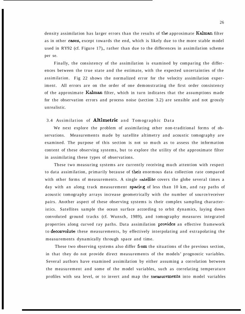
density assimilation has larger errors than the results of the approximate Kalman filter

as in other cases, except towards the end, which is likely due to the more stable model

used in RY92 (cf. Figure 17),, rather than due to the differences in assimilation scheme

per se.

Finally, the consistency of the assimilation is examined by comparing the differ-

ences between the true state and the estimate, with the expected uncertainties of the

assimilation. Fig 22 shows the normalized error for the velocity assimilation exper-

iment. All errors are on the order of one demonstrating the first order consistency

of the approximate Kalman filter, which in turn indicates that the assumptions made

for the observation errors and process noise (section 3.2) are sensible and not grossly

unrealistic.

3.4 Assimilation of Altimetric and Tomographic Data

We next explore the problem of assimilating other non-traditional forms of ob-

servations. Measurements made by satellite altimetry and acoustic tomography are

examined. The purpose of this section is not so much as to assess the information

content of these observing systems, but to explore the utility of the approximate filter

in assimilating these types of observations.

These two measuring systems are currently receiving much attention with respect

to data assimilation, primarily because of theil enormous data collection rate compared

with other forms of measurements. A single sateilite covers the globe several times a

day with an along track measurement spacirlg of less than 10 km, and ray paths of

acoustic tomography arrays increase geometrically with the number of source/receiver

pairs. Another aspect of these observing systems is their complex sampling character-

istics. Satellites sample the ocean surface according to orbit dynamics, laying down

convoluted ground tracks (cf. Wunsch, 1989), and tomography measures integrated

properties along curved ray paths. Data assimilation prcwides an effective framework

to deconvolute these measurements, by effectively interpolating and extrapolating the

measurements dynamically through space and time.

These two observing systems also differ f]om the situations of the previous section,

in that they do not provide direct measurements of the models’ prognostic variables.

Several authors have examined assimilation by either assuming a correlation between

the measurement and some of the model variables, such as correlating temperature

profiles with sea level, or to invert and map the me~surements into model variables

27

first, such as performing tomographic inversions prior to assimilation. This relation-

ship between measurement and model variables is only a superficial difference, and

estimation theory does not distinguish between them. All that is required to perform

estimation is the forward theoretical relationsltip between the model’s state variables

and what is observed, Eq (10), and the Kahnan filter readily treats these nontraditional

measurements on the s~e footing as direct measurements of the model state elements

themselves without intermediate inversions.

Pseudo altimetric measurements were made along a set of tracks shown in Fig 23.

To simtdate the repeat period of the satellite measurement and the existence of its

subcycles, the sea’ level observation points are alternated between the crosses and the

diamonds every 2-days. Although the SPEM model uses the rigid lid approximation,

pressure gradients along the surface can be diagnostically computed from the model

state and inverted for pressure. Sea level is in turn related to pressure by the hydrostatic

relation. Because of the model’s advective noulinearities, this functional relationship

between state variables and sea level is nonlinear. The observation operator, H’, was,

therefore, obtained by linearizing this relationship about the time-mean jet (x), as in

the derivation of the linearized state transition matrix (Section 2.2). Sea levels are as-

similated on alternating tracks (crosses and diamonds), and therefore the observation

matrix, H, is not time-invariant (section 2.1). Nevertheless, as an additional approxi-

mation, an asymptotic error was computed assuming that the observations are present

on both tracks simultaneously (but not during the actual filtering. ) The resulting sea

surface density evolution of the sea level assimilation is shown in Fig 24. As in previous

experiments, the meanders are resolved by the assimilation, and the actual errors are

greatly reduced from the “false ocean” (Fig 25). As a result of the added spatial cover-

age compared with the pseudo mooring assimilations in the previous section, the eddy

(H in Fig 4) in the eastern domain is suppressed in Fig 24. However, the southward

meander (C in Fig 4) is not resolved well, as it is not sampled by the altimetry tracks

(Fig 23).

In light of the analysis of density assimilation in section 3.3, tomographic measure-

ments of density (temperature) is not expected to be effective for the present simulation

either, because of the dominance of bakotropic. instability. Therefore, instead, we shall

examine pseudo reciprocal tomographic measurements in which mean velocity along

28

ray paths are assimilated. Fig 26 shows the array configuration for this pseudo recip-

rocal tomography, where there are 22 pairs of measurements. For simplicity, we shall

assume the ray paths to be horizontal and that measurements are available only at

mid-depth (2000 m), as opposed to actual multiple vertical ray paths between sources

and receivers. Velocity projections ontc) the rays were integrated along each pair in Fig

26 and assimilated every 2-days. The resulting sea surface density (Fig 27) shows the

meanders being resolved as in previous experiments. However, as the data are limited

to averages over long distances, some small scale differences from the “true ocean” are

more noticeable, in particular eddies 1% and E’ in Fig 27. Reductions of the relative

errors are shown in Fig 25. The smaller relative skill compared with other experiments

is due to the difference in the assimil~ted amount of information. For example, any

pair of stream function measurements provide similar information as do the pseudo re-

ciprocal tomography, but the” number of such pairs in the stream function experiment

is 325, as opposed to 22 for the present experiment.

4. Summary and Discussion

An approximate Kahnan filter was derived and successfully used for data assimilation

with an ocean general circulation model. The Inodel is an idealized Gulf Stream, and is

based on a nonlinear primitive equation model with a large dimension of over 170,000

state elements. The model has an unstable jet with an open horizontal boundary

and a rigid lid. The effectiveness of assimilating various types of pseudo observations

was examined includlng localized measurements of velocity, density, and volume trans-

port, and indirect measurements by pseudo sate~lte altimetry and acoustic tomography.

These examples are some of the most complex ocean models that have been analyzed

with estimation theory, in terms of the model’s algorithm, size, dynamics, and types of

measurements.

The approximate filter involves a state dimension reduction scheme based on a

spatio-dynamic transformation, an asymptotic steady-state error cova.riance matrix,

and a time-invariant linearized dynamic model for the Riccati equation. The filter was

shown to successfully estimate the model state, except for the case of density assimilw

tion, which proved relatively inefficient for the present simulation because of the jet’s

dominant barotropic instability and strong advective nordinearities. The assimilated

I 29

results were found to be more accurate than what was estimated using a simpler nudg-

ing scheme, except for density assimilation at the end of the experiment, which appears

to be “due to differences in the models employed. Despite the dramatic simplifications in

deriving the approximate filter, the results demonstrate that the filter retains sufficient

properties of the optimal solution to be useful.

The significance of the present study is several-fold. One, that a suboptimaJ

Kalman filter based on an approximate model error estimate was demonstrated to

generally outperform an empirical assimilation scheme (nudging). Two, that approxi-

mate model errors can be computed practically even for large complex general circula-

tion models by the proposed method. Formulation by estimation theory readily puts

complex observations such as altimetry and tomography on the same footing as other

direct measurements of the state variables, which otherwise are difficult to assimilate

by strictly empirical methods.

The computational requirements of the pI esent calculation is minimal. The most

time-consuming step turns out to be the numerical construction of the linearized coarse

state transition matrix, Eq (20). To minimize the necessary computations, the two-day

transition matrix was computed by first constructing an equivalent transition for six

hours and then multiplying this matrix with itself. Derivation of the six hour transition

matrix required 130 CPU minutes on a Cray Y/MP (2.6 Mw memory). (The matrix

multiplication to convert to a 2-day transition required a mere 18 CPU seconds.) The

computation of the asymptotic steady-state error is the largest computation besides

the transition matrix, which, for the present coarse dimension of 1399, required 7 Mw

of memory and 27 CPU minutes to perform 10 doubling iterations. (The doubling ac-●

tually converged around the eighth iterate.) Given the approximate Kalman filter, the

computational overhead of the actual filtering relative to a simulation is negligible, since

filtering only involves matrix-vector operations; both required approximately 20 Cray

Y/MP minutes to perform a 60-day integration. Many of the calculations deriving the

approximate filter are well suited for the emerging massively parallel supercomputers

and therefore can benefit greatly by their development. The computation of individual

columns of the state transition matrix is ‘independent among different columns and

therefore are completely parallelizable. The doubling algorithm is a recursive matrix

multiplication and inversion, for which parallel algorithms exist.

30

Virtually all practical assimilation schemes are approximations to the optimal esti-

mate, However, the implicit statistical assumptions are rarely discussed, nor estimates

of the final result’s accuracies provided. The pI esent approximate Kalman filter makes

these assumptions explicit for examination, and provides an approximate measure of ac-

curacy which is essential in evaluating the consistencies of the assumptions and testing

the vddity of the dynamic models (e.g., Fu et al., 1993).

The information content of various data types, or their effectiveness for estima-

tion, can be measured by examining the reduction in the estimate’s expected errors.

However, optimal observing system design is beyond the scope of the present study and

the results must properly be placed in context with regards to the model’s physics and

properties of the measurements, such as their amount and accuracies. For example,

although density measurements were found ineffective in the present simulation, such

would not likely be the case for a stable, oceanic condition, or if baroclinic instability y

were dominant. Error reduction also depends on the amount of assimilated data; for

example, there were 260 pseudo velocity merwurements as opposed to 26 for stream

function, There are two aspects to data error. One is the actual measurement error,

and the other is contributions from missing model physics. The former is obvious and

was not part of the identical twin experiment, but becomes a central issue in compari-

ng real observing systems. The latter, for the present simulation, is the small scale

variabilities unresolved by the coarse approxinlation, and the strong advective effects

of density. The effectiveness of data will be lessened if the effects of the unmodeled

physics on the measurements are large.

Observability characterizes one aspect of the data’s information content. However,

as demonstrated, although obse~bility pertains to whether the model state can be

constrained by the measurement, it does not indicate how well it will do so. An analysis

of the estimation errors, in particular, its reduction from the case without assimilation

is critical.

To first order, the error estimates of the present simulation were found to be con-

sistent with the actual errors. However, there are several indications that they are not

accurate. For example, figure 22 shows that actual errors are still decreasing with time

at the end of the experiment. Apparently, 60 days is too short for the estimation errors

to truly converge. Additionally, the normalized errors (Fig 22) suggest that baroclinic

velocity errors are overestimated whereas those for density are underestimated. We

31

have used the simplest model for the process noise, by ~suming that theY are un-

correlated among different state variables with ad hoc relative magnitudes. Although

the present approximation was demonstrated tc) be useful in estimation, more accurate

characterization of model process noise is needed.

The horizontal grid was made identicid between the barotropic and first baroclinic

modes. In retrospect, this is not an optimal c}loice, as baroclinic modes have smaller

horizontal length scales. Added resolution for the baroclinic mode would have increased

the computational cost due to the larger state dimension. However, if the small hor-

izontal scales can be approximated to be independent of processes at a distance, the

error covariances may be computed locally. Fo1 example, Parish and Cohn (1985) pro-

posed a band-limited approximation and algorithm for evaluating the error covariance

matrix. The possibility of combining the present reduced-dimension approximation and

a localized computation of the error covariance warrant further examination. Although

only filters have been explored in this study, the state reduction can easily be applied to

approximate smoothers as well. These and other issues including use of more realistic

process noise are left for future investigations.

32

Acknowledgements

Helpful discussions and suggestions to an earlier version of the manuscript by Lee-

Lueng Fu and Victor Zlotnicki are gratefully acknowledged. Roberta Young helped

set up the model for the simulations. This research was carried out in part by the

Jet Propulsion Laboratory, California Institute of Technology, under contract with

the National Aeronautics and Space Administration, PMR. was supported by NASA

through Grant #958208 (subcontract to MIT from JPL) and by the Office of Naval

Research, Grant NOO014-90-J-1481. Computations were performed on the Cray Y-MP

of the Supercomputing Project at the Jet Propulsion Laboratory.

—

33

References

Anderson, B. D. O., and J. B. Moore, 1979. “Optimal Filtering”, Prentice-Hall, Inc.,

Englewood Cliffs, N. J., 357 pp.

Bennett, A. F., and W. P. Budgell, 1987. Ocean data assimilation and the Kalrnan

filter: Spatial regularity, Journal of Physical Oceanography, 17, 1583-1601.

Fu, L.-L., L Fukumori and R. .N. Miller, 1993. Fitting dynamic models to the Geosat

sea level observations in the Tropical Pacific Ocean. Part II: A linear, wind-driven

model, Journal of Physical Oceanography, 23, 2162-2181.

Fukurnori, L, J. Benveniste, C. Wunsch and D. B. Haidvogel, 1993. Assimilation of sea

surface topography into an ocean circulation model using a steady-state smoother,

Journal of Physical Oceanography, 23, 1831-1855.

Gelb, A., 1974. “Applied Optimal Estimation”, M.I.T. Press, Cambridge, MA 374 pp.

Ghil, M., and P. Malanotte-Rizzoli, 1991. Data assimilation in meteorology and

oceanography, Advances in Geophysics, B. Saltzmann, cd., Academic Press, vol.

33, 141-266.

Goodwin, G. C., and K. S. Sin, 1984. “Adaptive Filtering Prediction and Control”,

Prentice-Hall, Inc., Englewood Cliffs, N. J., 540 pp.

Haidvogel, D. B., J. Wilkin and R. Young, 1991. A semi--spectral primitive equation

ocean circulation model using vertical sigma and orthogonal curvilinear coordinates,

Journal of Computational Physics, 94, 151-185.

Hautus, M. L. J., 1969. Controllability asld obscrvrrbilit y conditions of linear au-

tonomous systems, Proceedings of the Koninklijke Nederlandse Akademie van

Wetenschappen, Series A, 443-448.

Holland, W. R., and P. Malanotte-Rizzoli, 1989. Assimilation of altimeter data into an

ocean circulation model: space versus til ne resolution studies, Journa2 of Physica2

Oceanography, 19, 1507-1534.

Kindle, J. C., 1986, Sampling strategies and model assimilation of altimetric data for

ocean monitoring and prediction, Journal of Geophysical Research, 91, 2418–2432.

34

Malanotte-Rizzoli, P., and W. R. Holland, 1986. Data constraints applied to mod-

els of the ocean general circulation. Part I: the steady case, Journal of Physical

Oceanography, 16, 1665-1682.

Malanotte-Rizzoli, P., and W. R. Holland, 1988. Data constraints applied to models

of the ocean general circulation. Part II: the transient case, Journal of Physical

Oceanography, 18, 1093-1107.

Malanotte-llizzoli, P., R. E. Young, and D. B. Haidvc)gel, 1989. Initialization and data

assimilation experiments with a primitive equation model, Dynamics of A tmospheres

and Oceam, 13, 349–378.

Malanotte-Rizzoli, P., and R. E. Young, 1992. How useful are localized clusters of

traditional oceanographic measurements for data assimilation?, Dynamics of Atmo-

spheres and Oceans, 17, 23-61.

Marotzke, J., and C. Wunsch, 1993. Finding the steady state of a general circulation

model through data assimilation: application to the North Atlantic Ocean, Journa/

of Geophysical Research, 98, 20149-20167.

Marshall, J. 1985. Determining the ocean circulation and improving the geoid from

satellite altimetry, Journal of Physical Oceanography, 15, 330-349.

Martel, F., and C. Wunsch, 1993: The North Atlantic circulation in the early 1980s— An estimate from inversion of a finite difference model, Journal of Physical

Oceanography, 23, 898-924.

Mellor, G. L., and T. Ezer, 1991. A Gulf Stream model and an altimetry assimilation

scheme, Journal of Geophysical ReseaTch, 96, 8779-8795.

Miller, R. N., 1986. Toward the application of the Ka.lman filter to regional open ocean

modelling, Journal of Physics/ Oceanography, 16, 72-86.

Miller, R. N., and M. A. Cane, 1989. A Kalnmn filter analysis of sea level height in the

tropical Pacific, Journal of Physical Oceanography, 19, 773-790.

Moore, A. M., and D. L. T, Anderson, 1989. The a~similation of XBT data into a

layer model of the tropical Pacific Ocean, Dynamics of Atmospheres and Oceans,

13,441-464.

35

Orlanski, I., 1976. A simple boundary condition for unbounded hyperbolic flows.,

Journal of Computational Physics, 21, 251-269.

Parish, D. F., and S. E. Cohn, 1985. A Kalrnan filter for a two-dimensional shallow

water model: formulation and preliminary experiments, Ofice Note 904, National

Meteorological Center, Washington DC 20233, 64 pp.

Robinson, A. R., 1992. Shipboard prediction with a regional forecast model, Oceanog-

raphy, 1, 42-48,

Robinson, A. R. and W. Leslie, 1985. Estimation and prediction of oceanic eddy fields,

Progress in Oceanography, 14, 485--510:

Robinson, A. R., M. A. Span, L. J. Walstad, and W. G. Leslie, 1989. Data assimilation

and dynamical interpolation in Gulfcast experiments, Dynamics of Atmospheres and

Oceaw, 13, 301-316.

Semtner, A. J., and R. M. Chervin, 1992, C)cean general circulation from a global

eddy-resolving model, Journal of Geophysical Reseawh, 97, 5493–5550.

Sheinbaum, J., 1989. Assimilation of oceanographic data in numerical models, Ph.D.

thesis, University of Oxford, Oxford, England, 156 pp.

Smedstad, D. M., and J. F. O’Brien, 1991. Variational assimilation and parameter

estimation in an equatorial Pacific Ocean model, Progress in Oceanography, 26,

179-241.

White, W. B., C.-K. Tai, and W. R. Holland, 1990a. Continuous assimilation of Geosat

altimetric sea level observations into a numerical synoptic ocean model of the Cali-

fornia Current, Journal of Geophysical Research, 95, 3127--3148.

White, W. B., C.-K. Tai, and W. R, Holland, 1990b. Continuous assimilation of sim-

ulated Geosat altimetric sea level into an eddy-resolving numerical ocean model, 1.

Sea level differences, Journal of Geophysical Research, 95, 3219-3234.

White, W. B., C.-K. Tai, and W. R. Holland, 1990c. Continuous assimilation of sim-

ulated Geosat altimetric sea level into an eddy-resolving numerical ocean model, 2.

Referenced sea level differences, Journal of Geophysical Research, 95, 3235-3252.

Wunsch, C., 1989. Sampling characteristics of satellite orbits, Journal of Atmospheric

and Oceanic Technology, 6, 891–907.

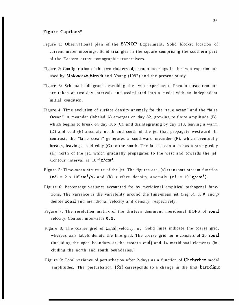
36

Figure Captions”

Figure 1: Observational plan of the SYNOP Experiment. Solid blocks: location of

current meter moorings. Solid triangles in the square comprising the southern part

of the Eastern array: tomographic transceivers.

Figure 2: Configuration of the two clusters of. pseudo moorings in the twin experiments

used by Malanot te-Rizzoli and Young (1992) and the present study.

Figure 3: Schematic diagram describing the twin experiment. Pseudo measurements

are taken at two day intervals and assimilated into a model with an independent

initial condition.

Figure 4: Time evolution of surface density anomaly for the “true ocean” and the “false

Ocean”. A meander (labeled A) emerges on day 82, growing to finite amplitude (B),

which begins to break on day 106 (C), and disintegrating by day 118, leaving a warm

(D) and cold (E) anomaly north and south of the jet that propagate westward. In

contrast, the “false ocean” generates a southward meander (F), which eventually

breaks, leaving a cold eddy (G) to the south. The false ocean also has a strong eddy

(H) north of the jet, which gradually propagates to the west and towards the jet.

Contour interval is 10-”5 g/cm3.

Figure 5: Time-mean structure of the jet. The figures are, (a) transport stream function

(c.i. = 2 x 10]3 cm3/s) and (b) surface density anomaly (c.i. = 10–5 g/cm3).

Figure 6: Percentage variance accounted for by meridional empirical orthogonal func-

tions. The variance is the variability around the time-mean jet (Fig 5). u, v, and p

denote zonal and meridional velocity and density, respectively.

Figure 7: The resolution matrix of the thirteen dominant meridional EOFS of zonal

velocity. Contour interval is 0.5.

Figure 8: The coarse grid of zonal velocity, u. Solid lines indicate the coarse grid,

whereas axis labels denote the fine grid. ‘l’he coarse grid for u consists of 20 zonal

(including the open boundary at the eastern encl) and 14 meridional elements (in-

cluding the north and south boundaries.)

Figure 9: Total variance of perturbation after 2-days as a function of Chebychev modal

amplitudes. The perturbation (6x) corresponds to a change in the first baroclinic

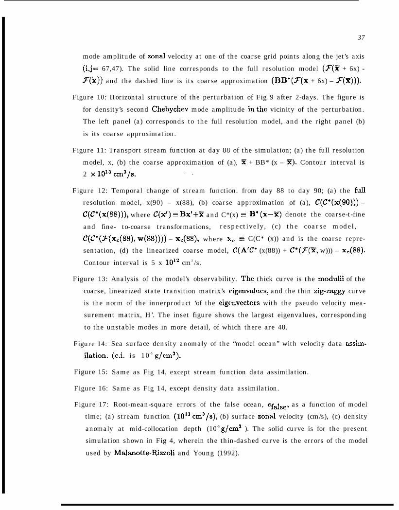
37

mode amplitude of zonal velocity at one of the coarse grid points along the jet’s axis

(i,j= 67,47). The solid line corresponds to the full resolution model (F(X + 6x) -

%(Z)) and the dashed line is its coarse approximation (BB”(7(x + 6x) – F(Y))).

Figure 10: Horizontal structure of the perturbation of Fig 9 after 2-days. The figure is

for density’s second Chebychev mode amplitude in the vicinity of the perturbation.

The left panel (a) corresponds to the full resolution model, and the right panel (b)

is its coarse approximation.

Figure 11: Transport stream function at day 88 of the simulation; (a) the full resolution

model, x, (b) the coarse approximation of (a), Y + BB* (x – x). Contour interval is

2 x 1013 cm3/s. .-

Figure 12: Temporal change of stream function. from day 88 to day 90; (a) the full

resolution model, x(90) – x(88), (b) coarse approximation of (a), C(C*(X(90))) –

C(C*(X(88))), where C(x’) s Bx’+x and C*(x) = 13” (x--x) denote the coarse-t-fine

and fine- to-coarse transformations, respectively, (c) the coarse model,

C(C*(X(X.(88), w(88)))) – xC(88), where x. - C(C* (x)) and is the coarse repre-

sentation, (d) the linearized coarse model, C(A’C* (x(88)) + C*(fi(X, w))) – xC(88).

Contour interval is 5 x 1012 cm3 /s.

Figure 13: Analysis of the model’s observability. The thick curve is the modulii of the

coarse, linearized state transition matrix’s eigenvalues, and the thin zig-zaggy curve

is the norm of the innerproduct ‘of the eigcnvectors with the pseudo velocity mea-

surement matrix, H’. The inset figure shows the largest eigenvalues, corresponding

to the unstable modes in more detail, of which there are 48.

Figure 14:

ilation.

Figure 15:

Figure 16:

Figure 17:

Sea surface density anomaly of the “model ocean” with velocity data assim-

(c.i. is 10-5 g/cm3).

Same as Fig 14, except stream function data assimilation.

Same as Fig 14, except density data assimilation.

Root-mean-square errors of the false ocean, ef~9e, as a function of model

time; (a) stream function (1013 cm3/s), (b) surface zonal velocity (cm/s), (c) density

anomaly at mid-collocation depth (10-5 g/cm3 ). The solid curve is for the present

simulation shown in Fig 4, wherein the thin-dashed curve is the errors of the model

used by Malanotte-llizzoli and Young (1992).

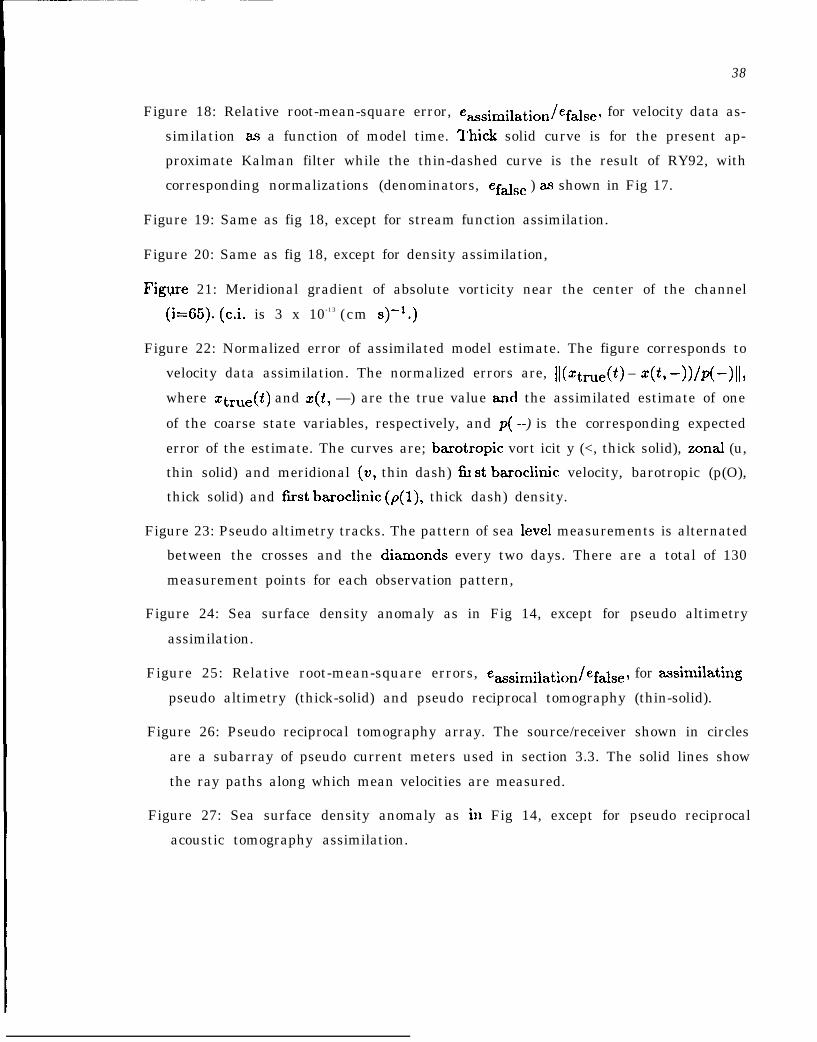
38

Figure 18: Relative root-mean-square error, eMsimilation/efal~e, for velocity data as-

similation as a function of model time. II’hick solid curve is for the present ap-

proximate Kalman filter while the thin-dashed curve is the result of RY92, with

corresponding normalizations (denominators, efd~e ) as shown in Fig 17.

Figure 19: Same as fig 18, except for stream function assimilation.

Figure 20: Same as fig 18, except for density assimilation,

Figue 21: Meridional gradient of absolute vorticity near the center of the channel

(i=65). (c.i. is 3 x 10-13 (cm S)-l.)

Figure 22: Normalized error of assimilated model estimate. The figure corresponds to

velocity data assimilation. The normalized errors are, Il(ztme(t) – z(t, –))/p(-)[1,

where ztrue(t) and z(t, —) are the true value ancl the assimilated estimate of one

of the coarse state variables, respectively, and p( --) is the corresponding expected

error of the estimate. The curves are; barotropic vort icit y (<, thick solid), zonal (u,

thin solid) and meridional (v, thin dash) fh st baroclinic velocity, barotropic (p(O),

thick solid) and first baroclinic (p(l), thick dash) density.

Figure 23: Pseudo altimetry tracks. The pattern of sea level measurements is alternated

between the crosses and the dkrnonds every two days. There are a total of 130

measurement points for each observation pattern,

Figure 24: Sea surface density anomaly as in Fig 14, except for pseudo altimetry

assimilation.

Figure 25: Relative root-mean-square errors, em9irni~ation/ef~se, for msifilating

pseudo altimetry (thick-solid) and pseudo reciprocal tomography (thin-solid).

Figure 26: Pseudo reciprocal tomography array. The source/receiver shown in circles

are a subarray of pseudo current meters used in section 3.3. The solid lines show

the ray paths along which mean velocities are measured.

Figure 27: Sea surface density anomaly as in Fig 14, except for pseudo reciprocal

acoustic tomography assimilation.

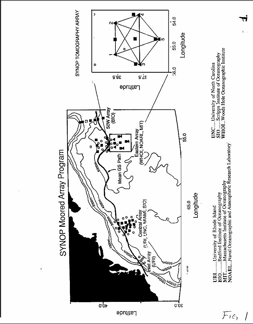
moz>m

,

w

\s’8f2

/

u )

o

Ooti

?r).

O“oc

L .

.

mj /

—

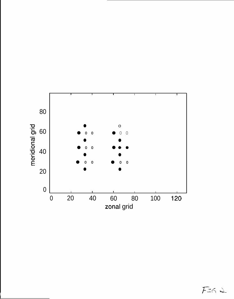
80

60

40d)E

20

0

●

● 0 0

●

● 0 0

●

● 0 0

●

o● 0 0

●

● 00

●

● 0 0

●

i I I I I I

1 1 1 1 1 1

0 20 40 60 80 100 120zonal grid

I

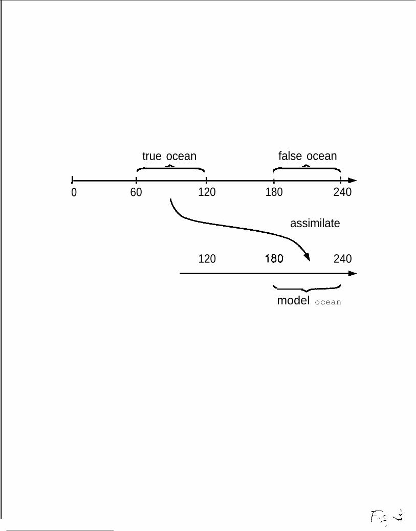
true ocean false oceanA AF T #- h

1 1 [ 1 i1 m u m b0 60 120 180 240

assimilate

120 180 240

\

model ocean

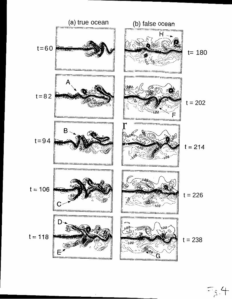
(a) true ocean (b) false ocean

t=60t= 180

LllllulJ ~UllLLUIIUlllUI

r’~11 ~Tmm)T,

t = 8 2t = 202

tI ~uululllululull

r l~TTTTmrrmrrr

t=94t=214

~wluulud

t=l18

t= 106

t = 226

t = 238

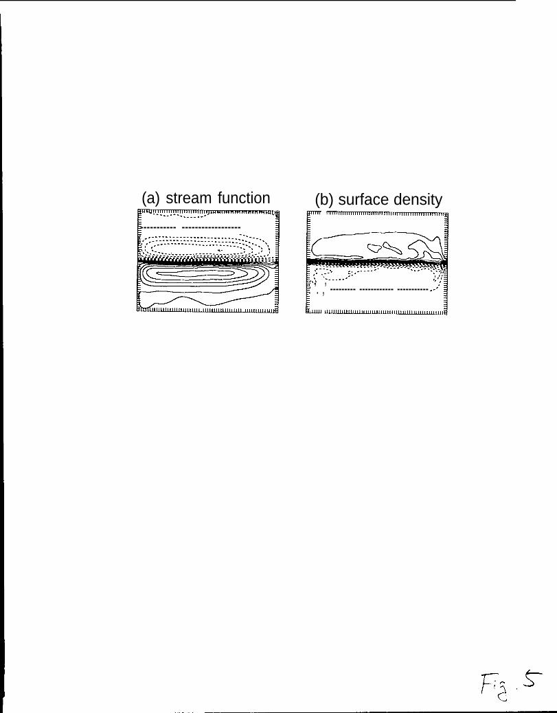
(a) stream function

----------- ------------------

(b) surface densityI mnmm??l~

. ’. ,’ --------- ------------ -----------UUUUMUllllllllllll.lull

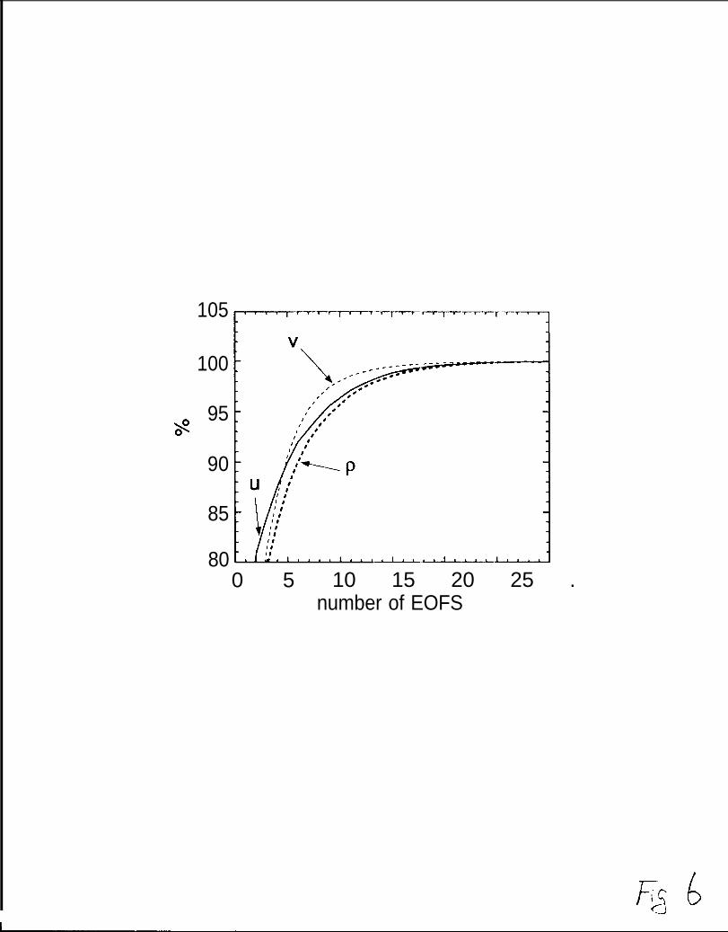
105

100

95

90

85

800 5 10 15 20 25 .

number of EOFS

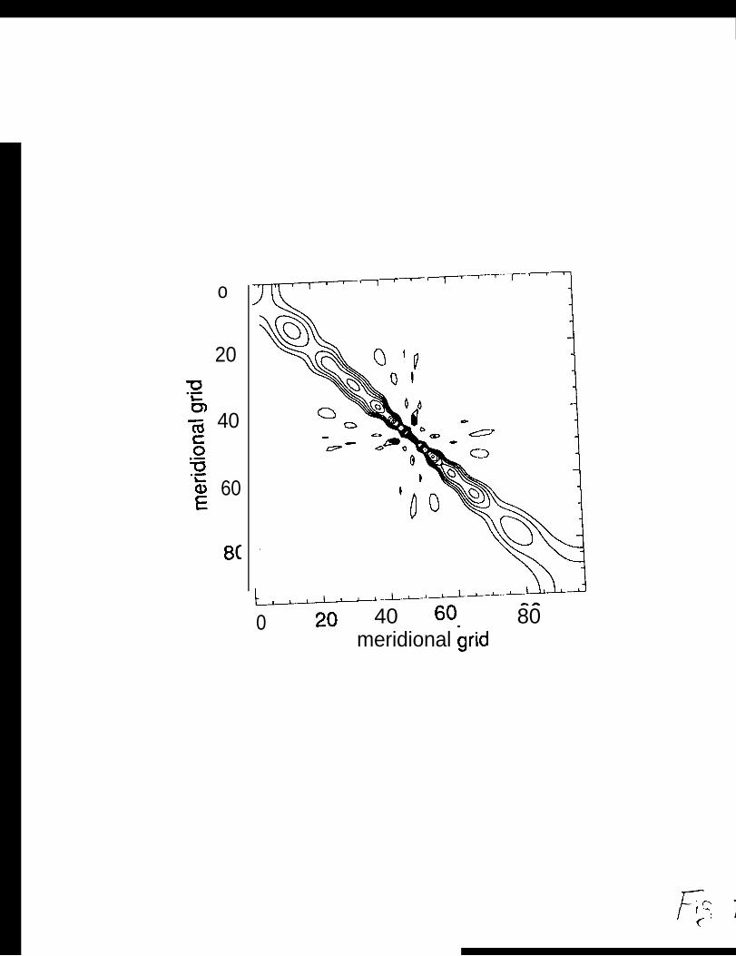
o

20

40

60

8[

t_--J-—’-”’~’L”—L——0 20 40 60, 80

meridional grid

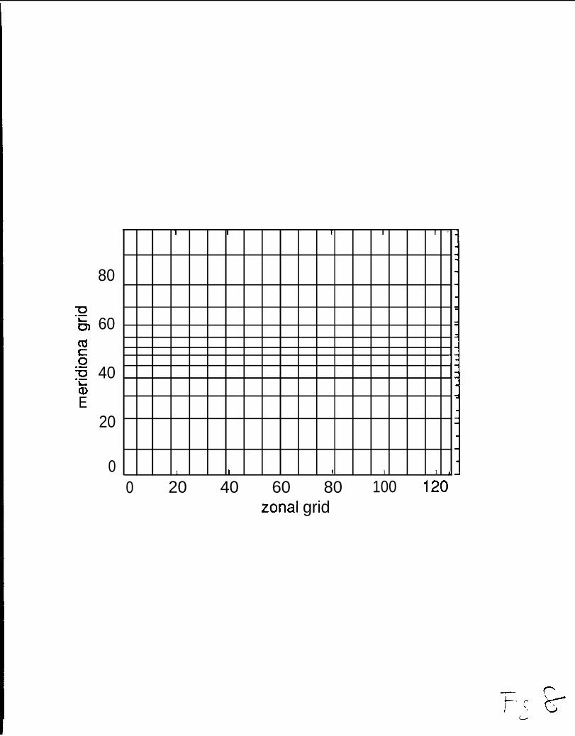
cdco.-a.-%E

80

60

40

20

0

I I 1 I I .

1

1

1 1 I 1 1 4

0 20 40 60 80 100 120zonal grid

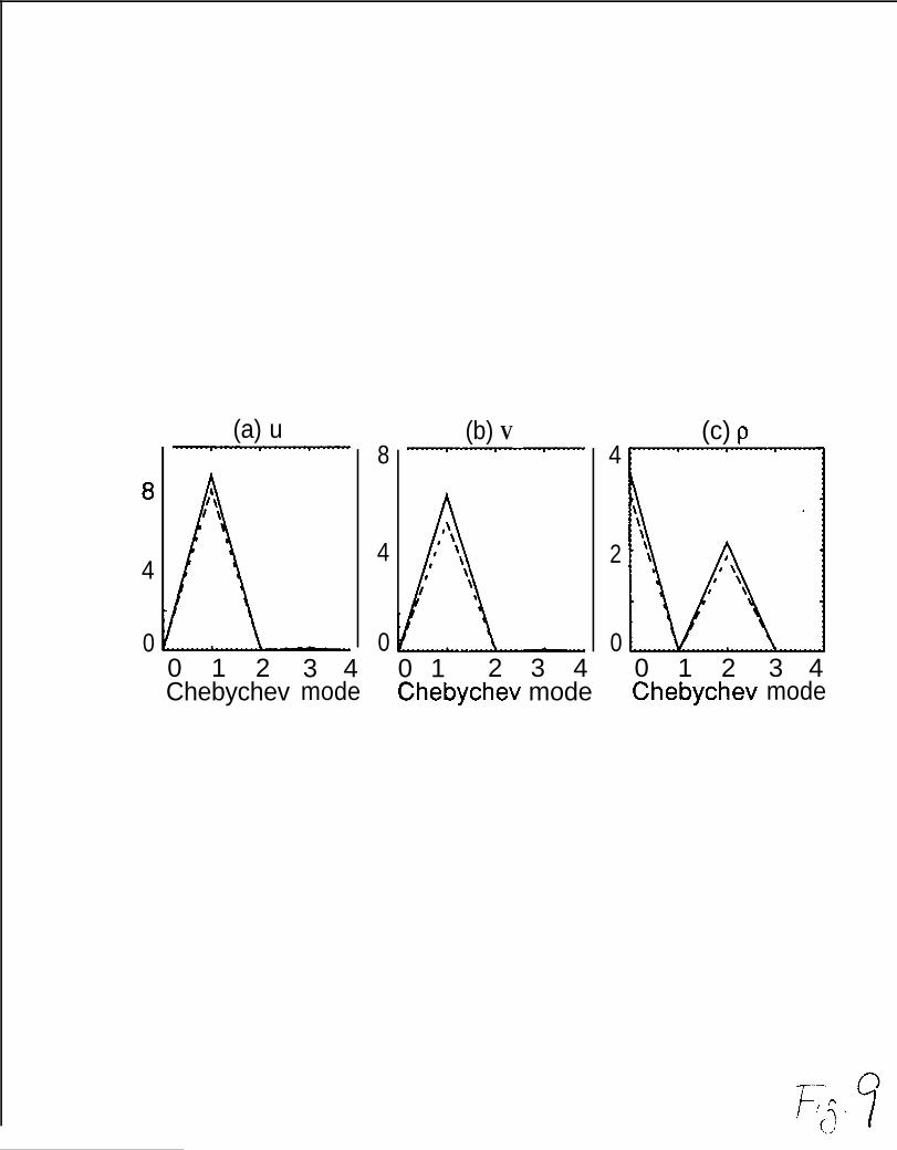
8

4

00 1 2Chebychev

3 4mode

(a) u8

4

0

(b) V

0 1 2 3 4Chebychev mode

4

2

0

(c) p

0 1 2Chebychev

3 4mode

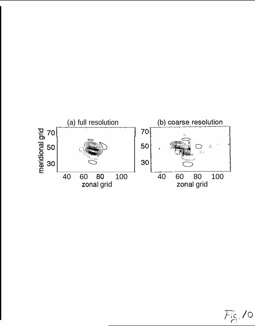
(a) full resolution

~1o

{:(?;$$>; :.b@#b. ..’-> “ ,,:; ::: . .‘. . ). . . .. . . . ..-

. . . . ...’

40 60 80 100zonal grid

1-50 , ‘@i’’’~!:: o ~; -

#.-.*‘..’1 - t.. ;4 ------~. .

30. ...-.’

l..—.-..4— - . 140 60 80 100

zonal grid

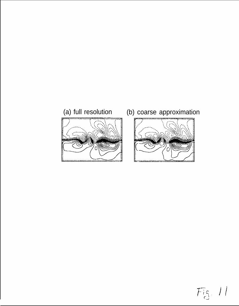
(a) full resolution (b) coarse approximation

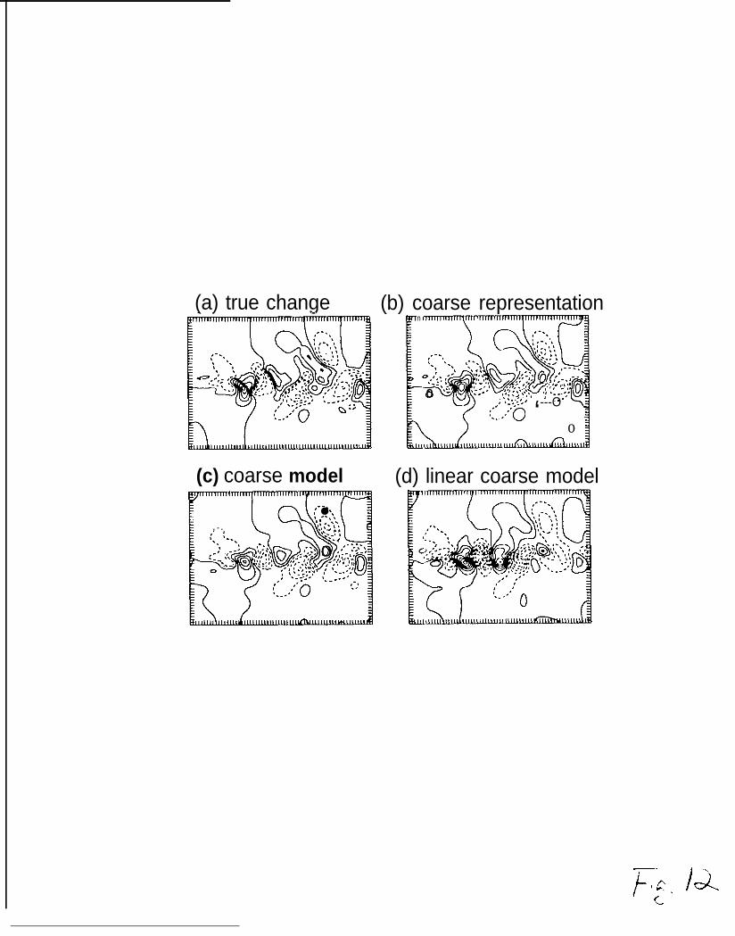
(a) true change. . —

(c) coarse model

w-. . .,’ ● ,‘, ,- ‘.,,,

, - . IQ ”.,,,:; + , ,,: .4,

‘., -.. ‘ .-. ,,-

3p,.,.~,--. D “:: o i::~’:: . . . ~ t’ ::; , ,--- ?,..,, .1, D,, ;: ,’=’1 ?,(:::/,‘.. . --- ,.’,’!’.-; y ,, ,.-.,~

?0 :::,:~<o’ ‘-”--’c”

(b) coarse representationn

*

. - .~ ,. :.,,,, ,,!,:,:.:, ,,.-.

‘.. ,-. ,‘. ..<

:, ‘:L’14,N ,,~::: o :!-:::‘.. :

-3e,,’,: ,.- .‘- -.,:, I,.; , ,.. ::

0 - ‘ “:; $;::;’:<’, ; ‘-:,’,’$.-.

‘::?;O ‘---O

o

(d) linear coarse model

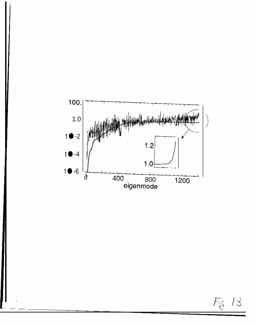
100,

1.0

1 ● -2

1 ● -4

1 ● -6‘1 l.o&-”

- 4 — — - . . L

J----l-~~~~o 400 800 1200

eigenmode

)

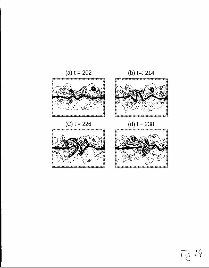
(a) t = 202

(C) t = 226

(b) t=: 214m IlnlmmmIlmnmn~

‘..’ . . . . .

(d) t = 238

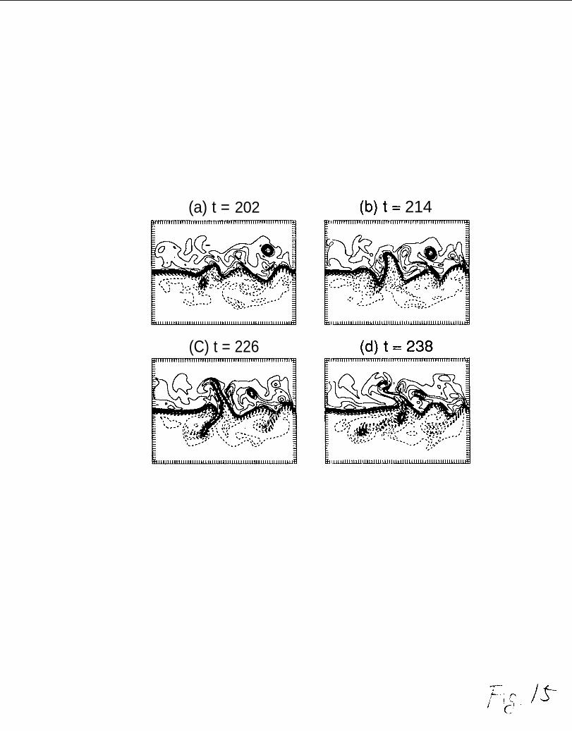
(a) t = 202

(C) t = 226

(b)t= 214mmlmmnTTrrlrm’m~

.,

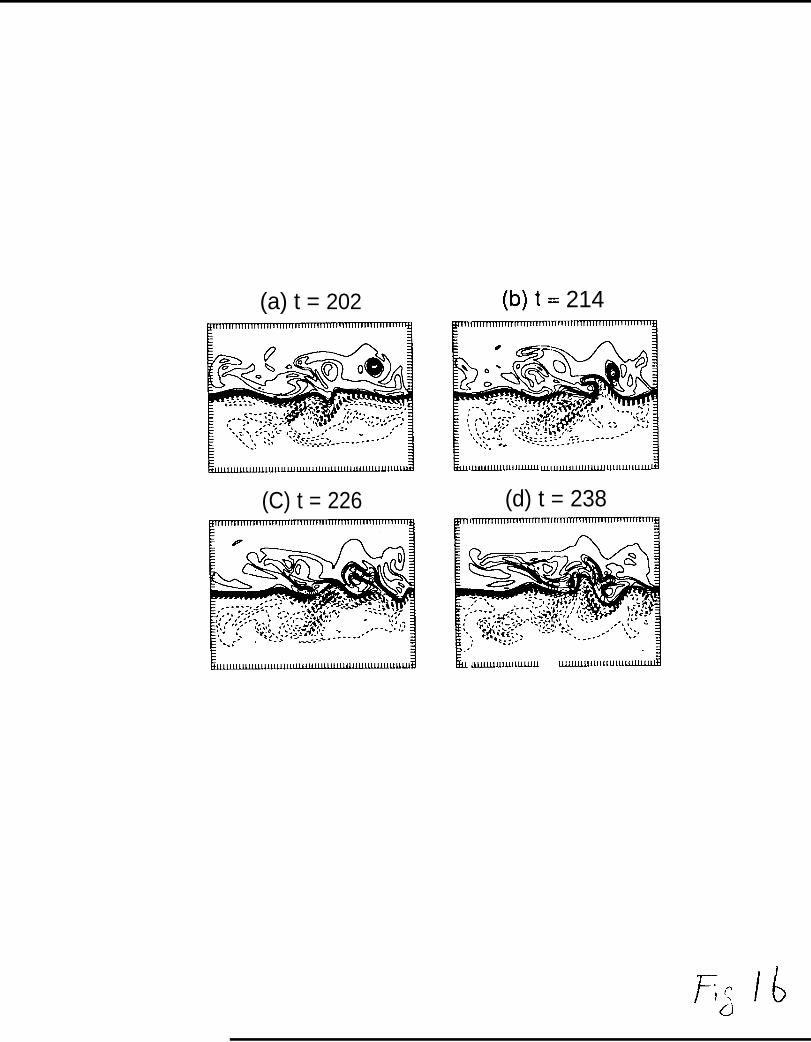
(a) t = 202

(C) t = 226

(b)t= 214mrnmmnnTrlTrmmnll~

. .

mluuuuuUILLLU ULLU~

(d) t = 238

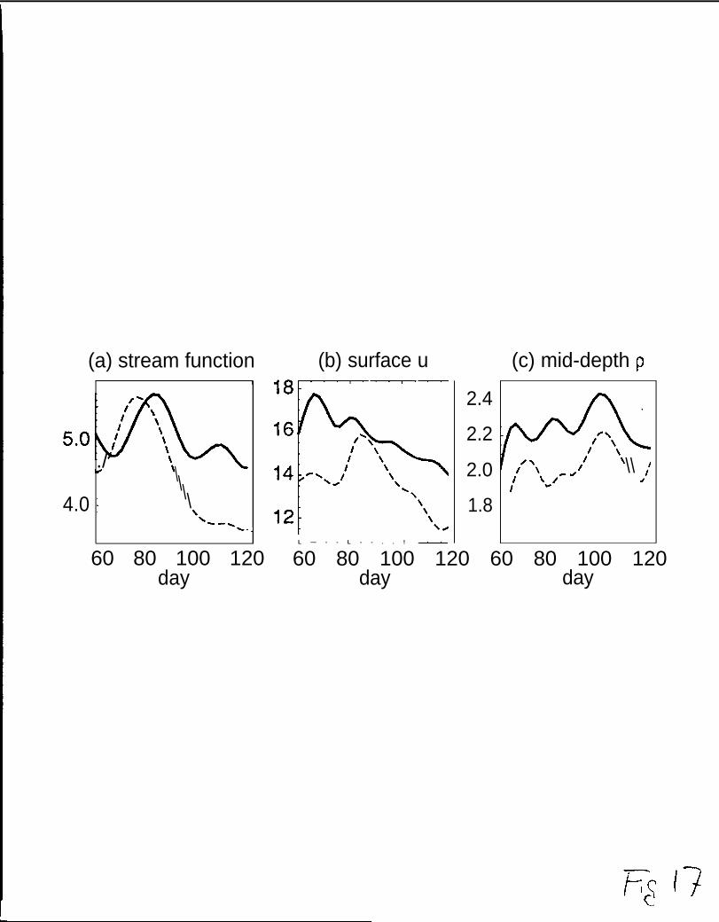
(a) stream function1

./\\

4.0 : \\\\+.. b,,

60 80 100 120day

(b) surface u

2.4

2.2

2.0

1.8

L — - - L - - . . ! —

(c) mid-depth p

O\ \

/\ /1 \\ j\“/* 4/’

60 80 100 120 60 80 100 120day day

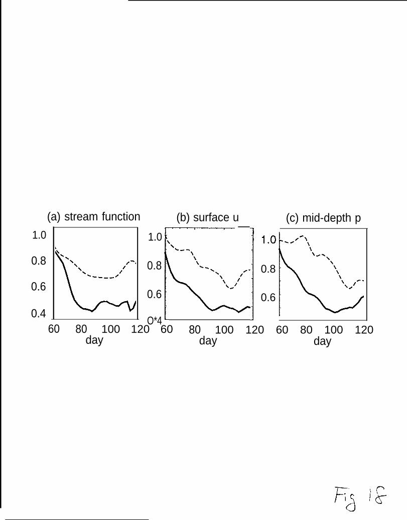
(a) stream function

1.0

0.8

0.6

0.460 80

1.0

0.8

0.6

(b) surface u—— —

day

O*4100 120 60

(c) mid-depth p

0.8

0.6

80 100 120 60 80 100 120day day

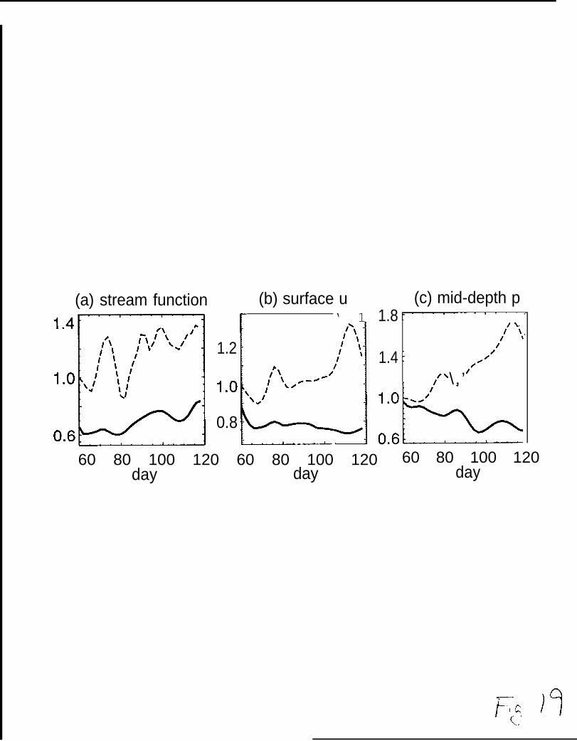
(a) stream function

1.2

1.0

0.8

(b) surface u‘ 1

—— f -1

(c) mid-depth p1.8 :“-’’-’”’””’”

// ‘1,,/1

1.4 ! ./’//\ Jt / \ , ’

60 80 100 120 60 80 100 120 60 80 100 120day day day

\.

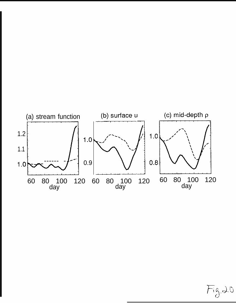
(a) stream functionr

1.2 ;

[1.1 :

------ -

1.0

0.9

60 80 100 120 60 80 100 120 60 80 100 120day day day

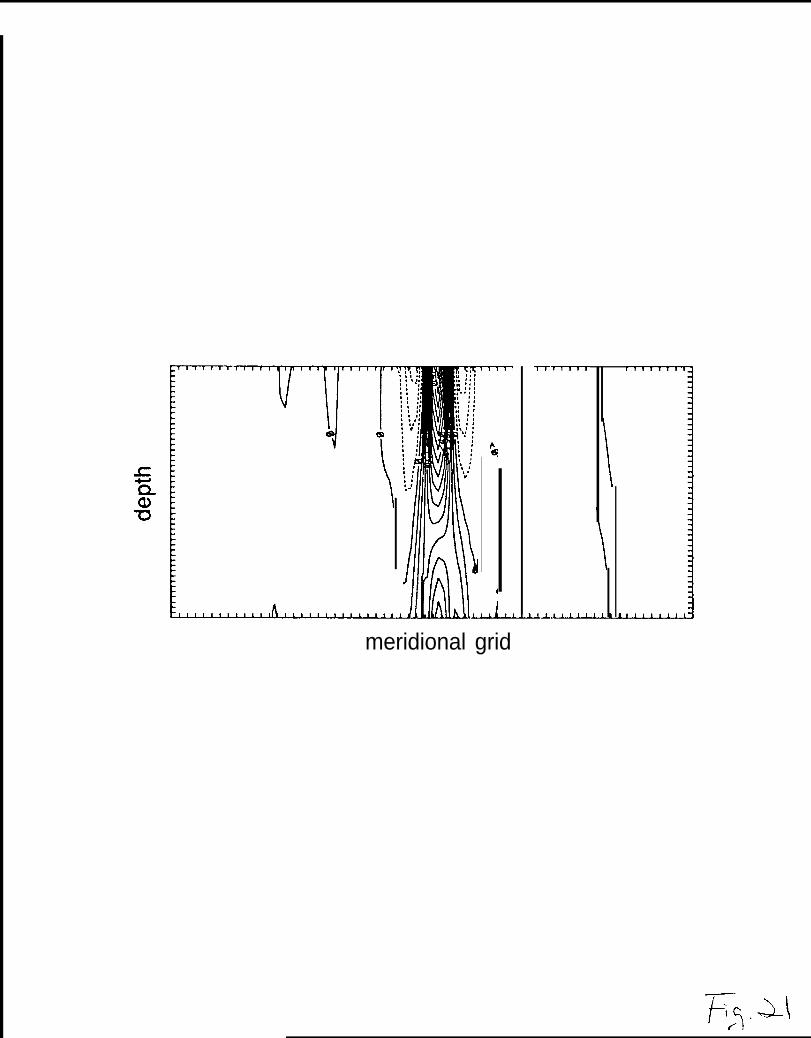
meridional grid

11—11—rt—r

J-LI...LLLULU

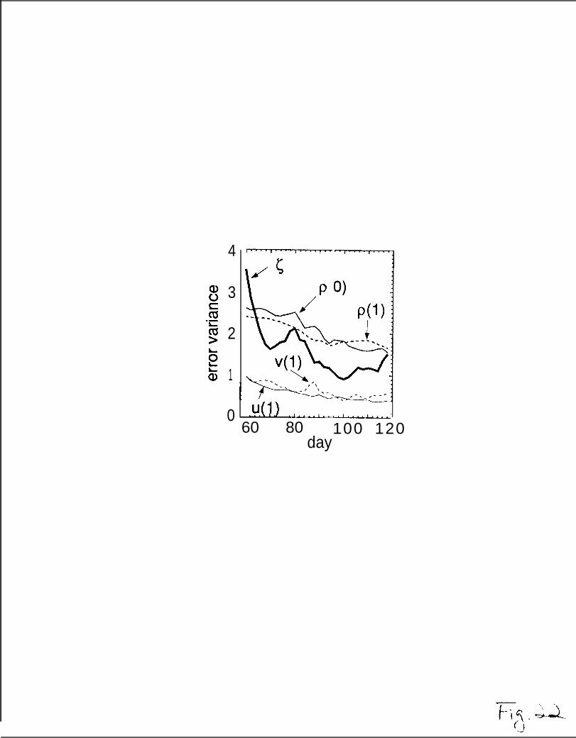
4

3

2

1

0.

u(j)%IJ ...1. . UJ+UAJ-I-U.”

60 80 100 120day

. +“

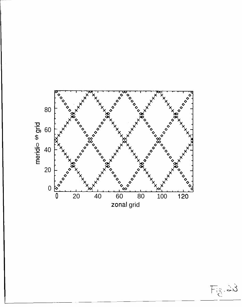
$0.—gii)E

80

60

40

20

00 20 40 60 80 100 120

zonal grid

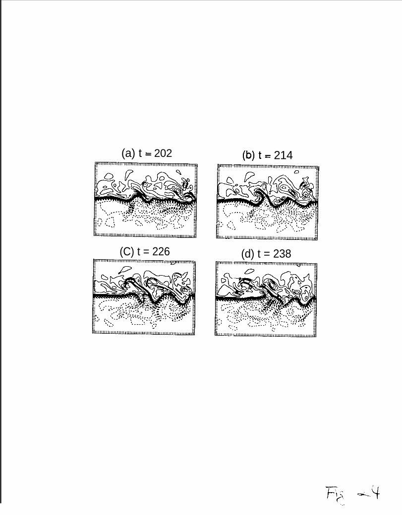
(a) t = 202

~L1.wuud

(C) t = 226

(b)t= 214

(d) t = 238

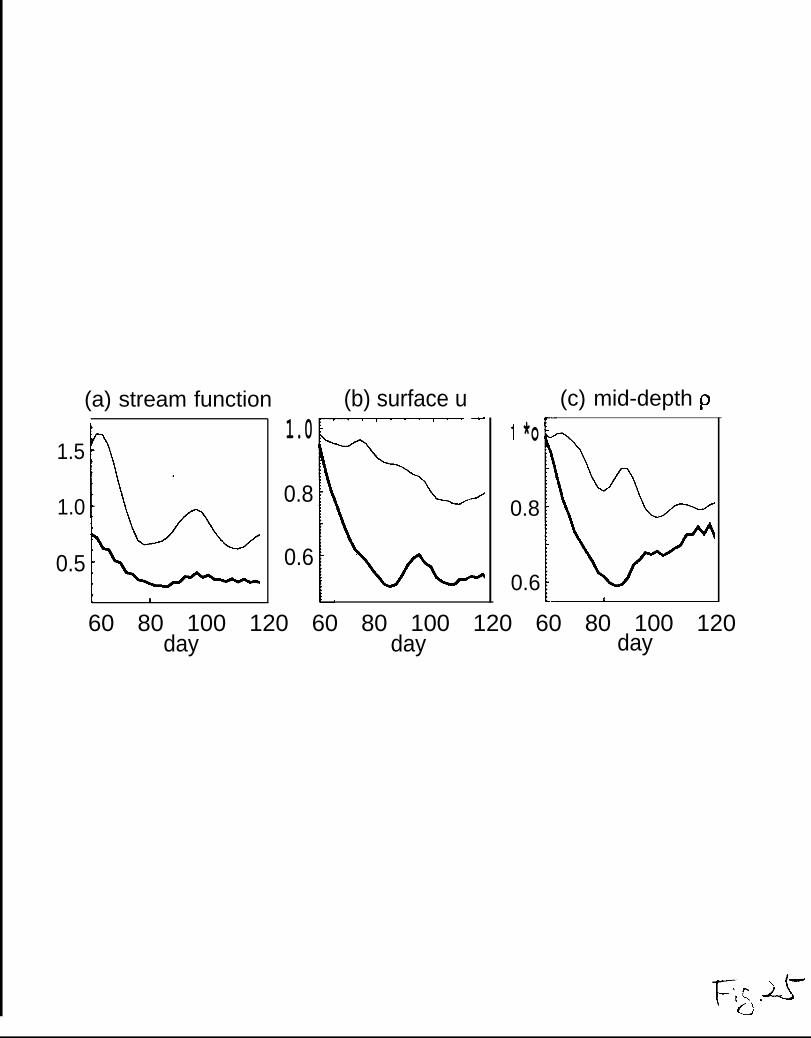
1.5

1.0

0.5

(a) stream function

t ,

1.0

0.8

0.6

(b) surface u—— -

1 *o

0.8

0.6

(c) mid-depth p

,

60 80 100 120 60 80 100 120 60 80 100 120day day day

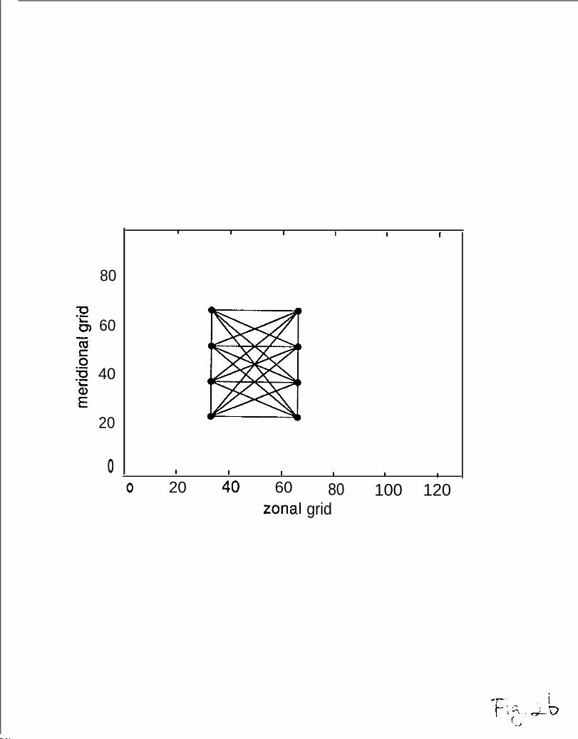
80

60

40

20

0

1 I I I 1 I

1 1 1 I 1 I

o 20 40 60zonal

80 100 120grid

——

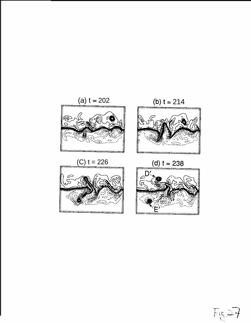
(a) t = 202

(C) t = 226

(b)t= 214