LNCS 4503 - Approximate Kalman Filters for Embedding Author-Word Co-occurrence …airoldi/pub/books/b01... · · 2008-04-14Approximate Kalman Filters for Embedding Author-Word Co-occurrence

Approximate Kalman Filters for EmbeddingAuthor-Word Co-occurrence Data over Time

Purnamrita Sarkar1, Sajid M. Siddiqi2, and Geoffrey J. Gordon1

1 Machine Learning Department,Carnegie Mellon University, Pittsburgh, PA 15213

{psarkar,ggordon}@cs.cmu.edu2 Robotics Institute,

Carnegie Mellon University, Pittsburgh, PA [email protected]

Abstract. We address the problem of embedding entities into Euclideanspace over time based on co-occurrence data. We extend the CODEmodel of [1] to a dynamic setting. This leads to a non-standard factoredstate space model with real-valued hidden parent nodes and discreteobservation nodes. We investigate the use of variational approximationsapplied to the observation model that allow us to formulate the entiredynamic model as a Kalman filter. Applying this model to temporalco-occurrence data yields posterior distributions of entity coordinates inEuclidean space that are updated over time. Initial results on per-yearco-occurrences of authors and words in the NIPS corpus and on syntheticdata, including videos of dynamic embeddings, seem to indicate that themodel results in embeddings of co-occurrence data that are meaningfulboth temporally and contextually.

1 Introduction

Embedding discrete entities into Euclidean space is an important area of researchfor obtaining interpretable representations of relationships between objects. Thisis very useful for visualization, clustering and exploratory data analysis. Recentwork [1] proposes a novel technique for embedding heterogeneous entities suchas author-names and paper keywords into a single Euclidean space based ontheir co-occurrence counts. When applied to the NIPS corpus, the resultingclusters of keywords and authors reflect real-life relationships between differentresearch areas and researchers in those respective areas. However, it would beinteresting to see how these relationships evolve over time, an aspect which thesetechniques do not address. Recent work has examined the dynamic behavior ofsocial networks [2], but only with homogeneous entities, and with point estimatesof the embedding coordinates. The problem we are interested in differs in twoways: first, embedding time-series co-occurrence data from two kinds of entities(essentially weighted link data from a bipartite graph) in a dynamic model couldbe useful for temporal data visualization, link prediction and group detection insuch networks. Examples of such bipartite data are author-word co-occurrences

E.M. Airoldi et al. (Eds.): ICML 2006 Ws, LNCS 4503, pp. 126–139, 2007.c© Springer-Verlag Berlin Heidelberg 2007

Kalman Filters for Embedding Co-occurrence Data over Time 127

in conference proceedings over time, actor-director collaborations throughouttheir careers, and so on. Second, modelling a distribution over the coordinates ofthese embeddings instead of point estimates (as in [2]) would tell us about thecorrelation and uncertainty in the entities’ coordinates. In this paper, we exploreone possible approach to achieve both these goals.

The layout of the rest of this paper is as follows. We discuss some relatedwork, in particular the model of [1] which we utilize. We then extend this modelto the dynamic case, describing how our dynamic model can be used for poste-rior estimation using a Kalman filter after some approximations. The resultingmodel keeps track of the belief state over all author and word coordinates in thelatent space based on the approximated co-occurrence observation model anda zero-mean Gaussian transition model. We give derivations and intuition forthe operation of this dynamic model, as well as results on the NIPS corpus ofauthor-word co-occurrence data and on synthetic data.

2 Related Work

The problem of embedding discrete entities into euclidean space is well-studied.Principal Components Analysis (PCA) is a standard technique based on eigen-decomposition of the counts matrix [3]. Multi-Dimensional Scaling (MDS) [4] isanother technique. However, these techniques are not suitable for temporal dataif one wishes to enforce smoothness constraints on embeddings over time.

[5] introduced a model similar to MDS in which entities are associated withlocations in p-dimensional space, and links are more likely if the entities are closein latent space. However their work does not take the sequential aspect of thedata into account. Also, the distribution over latent positions are obtained bysampling, which becomes intractable for large networks. Their work also assumesbinary link data.

The most closely related work is the CODE model of [1], which gives a tech-nique for embedding heterogenous entities (such as authors and keywords) basedon co-occurence data for the static case. We briefly introduce their model here,and our notation is similar to theirs.

The basic model of CODE is a conditional model p(w|a), where w denotesthe words and a denotes the authors. Let φi and ψj denote the hidden variablesrepresenting the coordinates of author ai and word wj in the latent space respec-tively. By Φt(A), Ψt(W ) we represent the states related to all author and wordpositions at timestep t. The conditional probability of seeing word wj given anauthor ai is related (inversely) to the distance dij = |φi − ψj | of author i andword j in the latent space, as well as the marginal counts of each individualentity, p̄(ai) and p̄(wj). For latent coordinates in a d dimensional space,

p(wj |ai) = p̄(wj)Z(ai)

e−|φi−ψj|2

Z(ai) =∑

wjp̄(wj)e−|φi−ψj |2

|φi − ψj |2 =∑d

k=1(φki − ψk

j )2(1)

128 P. Sarkar, S.M. Siddiqi, and G.J. Gordon

c11 c12 c21 c22

φ(a2)φ(a1)

ψ(w2)ψ(w1) C1

Φ(A1)

Ψ(W1)

C2

Φ(A2)

Ψ(W2)

Ct

Φ(At)

Ψ(Wt)

... ...

(A) (B)

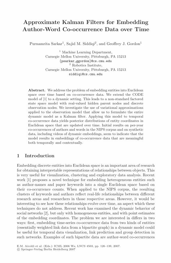
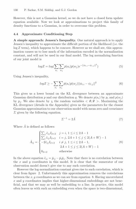
Fig. 1. Shaded nodes indicate hidden random variables. (A) The graphical model re-lating author/keyword positions to co-occurrence counts at a single timestep. (B) Thecorresponding factored state-space model for temporal inference.

The hidden coordinates Φt(A), Ψt(W ) are learned by maximizing the likelihoodobjective function using conjugate gradient or other such techniques.

3 The Single-Timestep Model

The original conditional model was chosen by considering p(w|a)p̄(w) to be inversely

proportional to the exponentiated squared distance between the latent embed-dings φ(a) and ψ(w). Similarly, our model of the joint is motivated by consideringthe initial ratio to be p(w,a)

p̄(w)p̄(a) instead, and deriving the resultant p(w, a) . Thereason for dividing by the empirical marginals is to normalize the joint by theoverall frequencies of the individual entities in the joint. This represents the sin-gle timestep graphical model shown in Figure 1(A). The resultant p(w, a) is asfollows:

p(ai, wj |φi, ψj) = 1Z p̄(ai)p̄(wj)e−|φi−ψj |2

Z =∑

ai

∑wj

p̄(ai)p̄(wj)e−|φi−ψj |2 (2)

4 Dynamic Embedding of Co-occurrence Data ThroughTime

We consider the unknown coordinates of authors and words to be hidden vari-ables in a latent space. Our goal is now to estimate these continuous hiddenvariables given discrete co-occurrence observations. As shown above, we modelthe joint posterior probability of author and word coordinates (given the obser-vations) based on the distances between those coordinates. To make the prob-lem tractable, we aim to derive a Gaussian distribution that is somehow closeto our observation model, which would allow us to use Kalman Filters, whichare described below. The natural approach which we follow is to minimize theKL-divergence of a Gaussian distribution (as an approximation to the obser-vation model) and the normalized likelihood of our model. However, this turnsout to be difficult since the KL-divergence has no closed-form solution, mainlydue to the non-standard log(Z) term (where Z is defined in equation (2). Weinvestigate two methods for making this expression tractable and obtaining a


Gaussian that approximates the observation model. We will see how the approx-imated model, together with a Gaussian transition model for the coordinates,can be formulated as a standard dynamic model.

4.1 The State-Space Model

For our state-space model in the dynamic setting, we choose a factored statespace model as shown in Figure 1(B), similar to a factorial HMM [6] or switchingstate space model [7]. It is a natural choice over the full joint model because weconsider the hidden coordinates of authors and words to be decoupled Markovchains conditionally coupled given their co-occurrence. This model closely re-sembles the factorial HMM model yet is distinct because of the hidden variablesbeing real-valued. Exact filtering and smoothing are very difficult in this modelbecause the prior belief state is not conjugate to the discrete observation densityfor typical belief distribution choices like the Normal distribution. Instead, wewould like to approximate this exact model in order to formulate it as a KalmanFilter.

4.2 Kalman Filters

A Kalman filter [8] is a linear chain graphical model with a backbone of hiddenreal-valued states emitting a real-valued observation at every timestep. Both theobservation and transition models are assumed to be Gaussian. It is commonlyused in tracking the states of complex systems or locations of moving objectssuch as robots or missiles. Filtering and smoothing are tractable in this modelbecause of the conjugacy of the Gaussian distribution to itself, which enablesthe belief state to remain Normally distributed at each timestep after the threestandard steps of conditioning (factoring in a new observation to the current be-lief state), prediction (propogating the belief through the transition model) androllup (marginalizing to obtain the new belief state). These steps are describedin more detail below.

4.3 Kalman Filter Formulation for Dynamic Embedding

In a standard Kalman Filter, all three steps mentioned above have closed formsolutions, i.e.:

Conditioning: P (Φt, Ψt|C1:t−1, Ct = ct)∝ P (Ct = ct|Φt, Ψt)P (Φt, Ψt|C1:t−1)

Prediction and Rollup: P (Φt+1, Ψt+1|C1:t)=

∫Φt

∫Ψt

P (Φt+1, Ψt+1|Φt, Ψt)P (Φt, Ψt|C1:t)∂Φt∂Ψt

(3)

These are the Kalman filter updates in our model. Lets see what happens forour model in the conditioning step. The observation model is:

log p(Ct|Φt, Ψt)= −

∑ai

∑wj

p̄(ai, wj)|φt,i − ψt,j |2 − log Z(4)


However, this is not a Gaussian kernel, so we do not have a closed form updateequation available. Now we look at approximations to project this family ofdensity functions to a Gaussian, in order to overcome this problem.

4.4 Approximate Conditioning Step

A simple approach: Jensen’s Inequality. One natural approach is to applyJensen’s inequality to approximate the difficult portion of the likelihood (i.e. thelog Z term), which happens to be concave. However as we shall see, this approx-imation causes us to lose much of the information encoded in the normalizationconstant, and will not be used in our final model. The log normalizing functionof our joint model is

logZ = log(∑

ai

∑

wj

p̄(ai)p̄(wj)e−||φt,i−ψt,j ||2) (5)

Using Jensen’s inequality,

logZ ≥ −∑

ai

∑

wj

p̄(ai)p̄(wj)||φt,i − ψt,j ||2 (6)

This gives us a lower bound on the KL divergence between an approximateGaussian distribution p and our distribution q. We denote p(ai) by pi and p(wj)by pj. We also denote by χ the random variables < Φ, Ψ >. Maximizing theKL divergence (details in the Appendix) gives us the parameters for the closestGaussian approximation to our observation model with mean zero and covarianceΣ given by the following equation.

Σ−1 = 2Λ̂ (7)

Where Λ̂ is defined as follows:

Λ̂ij =

⎧⎪⎪⎪⎪⎪⎪⎨

⎪⎪⎪⎪⎪⎪⎩

∑j c̃ijI2×2 j = i, 1 ≤ i ≤ 2A − 1

∑i c̃ijI2×2 i = j, 2A + 1 ≤ j ≤ 2(A + W ) − 1

−2c̃ijI2×2 i �= j, 1 ≤ i ≤ 2A − 1,2A + 1 ≤ j ≤ 2(A + W ) − 1

02×2 otherwise

(8)

In the above equation c̃ij = p̄ij − p̄ip̄j . Note that there is no correlation betweenthe x and y coordinates in this model. It is clear that the numerator of ourobservation model doesn’t give rise to any such correlation.

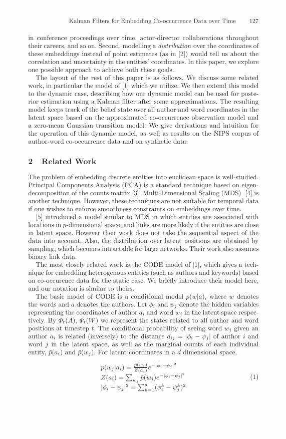
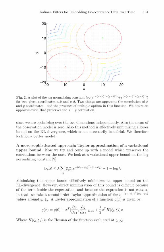
However the log-normalization constant gives rise to such correlation, which isclear from figure 2. Unfortunately this approximation removes the correlationsbetween the x, y coordinates as we can see from equation 8. Having uncorrelatedx and y coordinates implies that higher-dimensional embeddings are not bene-ficial, and that we may as well be embedding to a line. In practice, this modeloften leaves us with such an embedding even when the space is two-dimensional,


−20 −10 0 10 20−20

−10

0

10

20

x

y

Fig. 2. A plot of the log normalizing constant log(e(−(x−a)2−(y−b)2)+e(−(x−c)2−(y−d)2))for two given coordinates a, b and c, d. Two things are apparent: the correlation of xand y coordinates , and the presence of multiple optima in this function. We desire anapproximation that preserves the x − y correlation.

since we are optimizing over the two dimensions independently. Also the mean ofthe observation model is zero. Also this method is effectively minimizing a lowerbound on the KL divergence, which is not necessarily beneficial. We thereforelook for a better model.

A more sophisticated approach: Taylor approximation of a variationalupper bound. Now we try and come up with a model which preserves thecorrelations between the axes. We look at a variational upper bound on the lognormalizing constant [9].

log Z ≤ λ∑

ij

pipje−(φi−ψj)T (φi−ψj) − 1 − log λ

Minimizing this upper bound effectively minimizes an upper bound on theKL-divergence. However, direct minimization of this bound is difficult becauseof the term inside the expectation, and because the expression is not convex.Instead, we take a second order Taylor approximation of the e−(φi−ψj)T (φi−ψj)

values around ξi, ξj . A Taylor approximation of a function g(x) is given by,

g(x) = g(0) + xT [∂g

∂x1,

∂g

∂x2]ξi,ξj +

12xT H(ξi, ξj)x

Where H(ξi, ξj) is the Hessian of the function evaluated at ξi, ξj .


Now we have a Gaussian approximation to our observation model, whichhas canonical parameters Λ, η. These parameters , as derived in the appendix,are functions of the Jacobian and Hessian matrix of the taylor approximation,evaluated at ξi, ξj . We shall describe how we choose these parameters later inthis section.

In (3), we multiply two Gaussians i.e. prior p(Φt, Ψt|C1:t−1) with canonicalparameters (ηt|t−1, Λt|t−1) and the approximate observation distribution withη, Λ. The notation ηt|t−1 denotes the value of a parameter at time t conditionedon observations from timesteps 1 . . . t − 1. The resulting Gaussian p(Φt, Ψt|C1:t)is distributed with ηt|t, Λt|t, where

ηt|t = ηt|t−1 + η

Λt|t = Λt|t−1 + Λ

We compute the moment parameters μt|t, Σt|t from the canonical parameters.And we get the ηt|t−1, Λt|t−1 from the previous time-step of the Kalman Filter.

When applying the Taylor expansion, we set the ξ values to the μt|t−1 learntfrom the previous timestep. We found this to be most effective, and this also makessense since given the former time-steps’ data we are most likely to be around theconditional means predicted from the former time-steps. Because of the noncon-vex structure of the log-normalizer, which is due to the presence of saddle points(Figure 2), the resulting Λ can become non-positive definite and have negativeeigenvalues. To project to the closest possible positive definite matrix, we set thenegative eigenvalues to zero (plus a small positive constant). Together these ap-proximations succeed in giving us a tractable expressionwhile not losing the highlyinformative inter-coordinate interactions (e.g. x-y correlation in two dimensions)that the simple Jensen’s inequality approach would discard.

4.5 Prediction and Rollup Step

Our transition model is very simple, just a zero-mean symmetric increase inuncertainty:

(Φt+1, Ψt+1) = (Φt, Ψt) + N(0, Σtransition)

Here Σtransition is a diagonal noise term denoting the spread of uncertainty alongboth axes, which must be fixed beforehand. The prediction and rollup steps givethe following result:

(Φt+1, Ψt+1) ∼ N(μt+1|t, Σt+1|t)

where μt+1|t = μt|t and Σt+1|t = Σt|t + Σtransition.

4.6 Computational Issues

Note that we model all author-word interactions with a single large Kalmanfilter, where the authors and words relate through the covariance matrix. Thisintroduces complexity issues since the size of the covariance matrix is propor-tional to the number of authors and words. However some sparseness propertiesof the covariance matrix can be exploited for faster computation.


−2 −1.5 −1 −0.5 0 0.5 1 1.5 2−2

−1.5

−1

−0.5

0

0.5

1

1.5

2

A

A

A

B

B

B

X

XX

YY

Y−2 −1.5 −1 −0.5 0 0.5 1 1.5 2

−2

−1.5

−1

−0.5

0

0.5

1

1.5

2

A

AA

BB

B

XXXYYY

(A) (B)

−2 −1.5 −1 −0.5 0 0.5 1 1.5 2−2

−1.5

−1

−0.5

0

0.5

1

1.5

2

A

A

A

B

B

BX

X

X

YY

Y

1.4 1.6 1.8 2 2.2 2.4 2.6 2.8.5

2

.5

3

A

A

A

B

B

B

XXX

YY

Y

(C) (D)

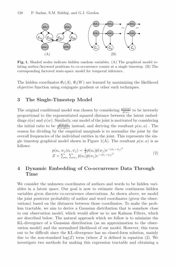
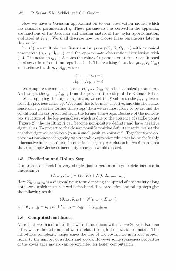
Fig. 3. Dynamic embedding of synthetic data vs. static embedding. A, B are two groupsof authors and X, Y are two groups of words. The 140-timestep data smoothly variesfrom strong A-X and B-Y links to strong A-Y and B-X links. The entities are initializedrandomly (not shown). A. t = 20, strong A-X and B-Y links. B. t = 70, Intermediateconfiguration, noisy uniform links. C. Strong A-Y and B-X links. D. A static embeddingof the aggregate co-occurrence matrix, which is effectively a noisy uniform matrix,resulting in entities mixing with each other.

5 Experiments

We divide the results section in three parts. We present some snapshots fromour algorithm on embeddings of a synthetic datasets with pre-specified dynamicstructure. We then present snapshots and closeups of embeddings of author-wordco-occurrence data from the NIPS corpus over thirteen years. We also showhow the distance in our embedding between author-word pairs in the corpusevolve over time. In all cases, Σtransition is currently set heuristically to givea smoothly varying embedding that is still responsive to new data. We finishour experimental section with a comparison with PCA [3], a well-studied staticembedding technique.

5.1 Modeling Trends over Time

We wish to inspect the performance of dynamic embedding in cases where theunderlying model is known. To do this, we generate noisy co-occurrence matricesof 3 words and 3 authors over 140 timesteps. The matrices have some amount


−2 −1.5 −1 −0.5 0 0.5 1 1.5.5

−1

.5

0

.5

1

.5

SejnowskiT

KochC

JordanM

HintonG

MozerM

SinghS

BengioY

SmolaA

DayanP

GilesC

DenkerJ

ScholkopfB

BartoA

MorganN

ObermayerK LeCun

YSimardP

ZemelR

GuyonI

WaibelA

TrespV

KawatoM

WilliamsC

BowerJ

MullerK

PougetA

GhahramaniZ

LeeY

StorkD

VapnikV

LippmannR

HendersonD

SunG

JackelL

GrafH

MurrayA

MoodyJTishby

N

ViolaP

SaadD

networklearningmodelneural

593datafunction

figuretime

set

networks

trainingalgorithmoutput

numbersystemerrorstate

units

information

models

hidden

performancespace

weights

linearlayer

vector

order

probability

parametersnoiseweight

functions

neurons

unitdistribution

recognition

method

approach

image

control

localneuron

rate

test

patterns

matrix

optimal

signalgaussian

visual size

feature

nettask

methodscellsfeatures

process

level

current

memoryresponse

architecture

equationfixed

line

images

speechstates

termvariablessolution

log

sequencedynamics

initial

distance

connections

node

direction

mapphase

machine

object motion

positionbasisdensity

analog

component

decisioncontext

hand

circuit

stimulusrecurrent

search classifier

word

parttheorem

bound

firing

cortex

spike

tree

distributedbayesian

equations

chip

markov

regionforwardscaletasksmeans

reinforcement

factor

orientation

policy

em

eye

motor

cortical

brain

voltage

contrastconnectionupdate

support

dependent

sourcewords

code

kernel

graph

sequencesdomain

solutions

trajectory

capacity

classifiers

statistics

channel

clustering

velocity

controller

entropy

path

associative

inverse

rbf

synapse

adaptation

development

jordan mlp

character

segmentation

empiricalcall

filters

experts

attention

population

resolutionmovement

lateral side

trees

teacher

module

speaker

matchpca

address

chain

grid

risk

arm

parts

digital

flow

competitive

tangent

interactionsweak

temperature

regularization

pulse

characters

attractor digitann

pruning

student

missingtext

agent

competition

codes

ocular

evolution

centers

centeredmargin

delays

normalization

false

visible query

faces

templatekernels

dominance

retrieval

weighting

subspace

modes

committee

tdnn

miller

cun

return

cue

boarddisparity

routing

variational

lgn

pathway

facial

recognizerimpulse

vor

critic

convolution

growing

adaboost

interneurons

obs

directional

actor

optpitch

composite

hme

documents

price

prototypes

stackhyperparameters

findings

conditioning

sharing

acquisition

tresp

sv

drift

signature

binocular

hit

obd

mouse

schedulesparietal

fitness

trading

aircraft

warpingsignatures

writer

statisticmimic

overcomplete

rivalry

mst

anna

repetition

synergy

tags

occupancy

sex

acetylcholine

tit

manager

rap

−1.6 −1.4 −1.2 −1 −0.8 −0.6

.3

.4

.5

.6

.7

.8

.9

MozerM

SmolaA

ScholkopfB

ObermayerK

WilliamsC

BowerJ

TishbyN

data

function

setalgorithm

numbererror

information

vector

functions

ratepatterns

level

partbound

cortextree

markovorientation

eye

corticalcontrast

kernel

clustering

entropy

adaptation

attention risk

parts

regularization

competition

ocular

kernels

dominance

pathway

stack

hyperparameters

sv

tags

occupancy

(A) (B)

−0.2 0 0.2 0.4 0.6 0.80.4

0.5

0.6

0.7

0.8

0.9

1

1.1

1.2

1.3

1.4

SinghS

DayanP

BartoA

VapnikV

GrafH

MoodyJ

rate

feature

cells

features

theorem

reinforcement

policy

supportcapacity

call

competitive

agent

committee

miller

return

routing

critic

actor

composite

price

conditioning

acquisition

binocular

trading

rivalry

synergy

−0.3 −0.2 −0.1 0 0.1 0.2 0.3

0.2

.15

0.1

.05

0

.05

0.1

.15

0.2

SejnowskiT

KochC

JordanM

HintonGMozer

M

SinghS

BengioY

SmolaA

DayanP

GilesC

DenkerJ

ScholkopfB

BartoA

MorganN

ObermayerK

LeCunY

SimardP

ZemelR

GuyonI

WaibelA

TrespV

KawatoM

WilliamsC

BowerJ

MullerK

PougetA

GhahramaniZ

LeeY

StorkD

VapnikV

LippmannRHenderson

DSun

G

JackelL

GrafH

MurrayA

MoodyJ

TishbyN

ViolaP

SaadD

network

learning

model

neural

593

data

functionfigure

timeset

networkstraining

algorithm

output

numbersystem

error

state

units

information

models

hidden

performance

space

weights

linear

layer

vector

order

probability

parameters

noise

weight

functionsneurons

unitdistribution

recognition

methodapproachimagecontrol

localneuron

ratetest

patternsmatrix

optimalsignalgaussian

visual

size

feature

net

task

methods

cells

featuresprocess

level

current

memory

response

architecture

equationfixedline

images

speech

states

termvariables

solution

log

sequence

dynamicsinitialdistance

connectionsnode

directionmapphase

machine

object

motion

positionbasis

densityanalog

component

decision

context

hand

circuit

stimulus

recurrentsearch

classifier

word

parttheorembound

firing

cortex

spike

tree

distributedbayesianequationschipmarkovregion

forward

scale

tasksmeans

reinforcement

factor

orientation

policyem

eye

motor

cortical

brain

voltagecontrast

connection

update

support

dependent

source

words

code

kernel

graphsequencesdomainsolutions

trajectory

capacity

classifiers

statisticschannel

clustering

velocity

controller

entropy

path

associativeinverserbf synapseadaptationdevelopment

jordan

mlpcharactersegmentation

empirical

call

filters

experts

attentionpopulationresolutionmovement

lateralsidetreesteacher

module

speaker

match

pca

address

chain

gridrisk

armpartsdigital

flow

competitivetangent

interactionsweaktemperature

regularization

pulse

characters

attractordigitann

pruningstudentmissing

textagent

competition

codes

ocular

evolutioncenters

centered

margin

delaysnormalizationfalsevisiblequery

faces

template

kernelsdominance

retrievalweightingsubspacemodescommittee

tdnn

miller

cun

returncueboard

disparity

routingvariational

lgnpathway

facial

recognizer

impulse

vor

criticconvolutiongrowing

adaboost

interneurons

obsdirectionalactoropt

pitchcomposite

hme

documentspriceprototypes

stack

hyperparametersfindingsconditioning

sharingacquisitiontresp

sv

drift

signature

binocularhitobd

mouse

schedules

parietal

fitnesstradingaircraft

warpingsignatureswriter

statisticmimicovercompleterivalrymst

annarepetitionsynergy

tagsoccupancy

sexacetylcholinetitmanager

rap

(C) (D)

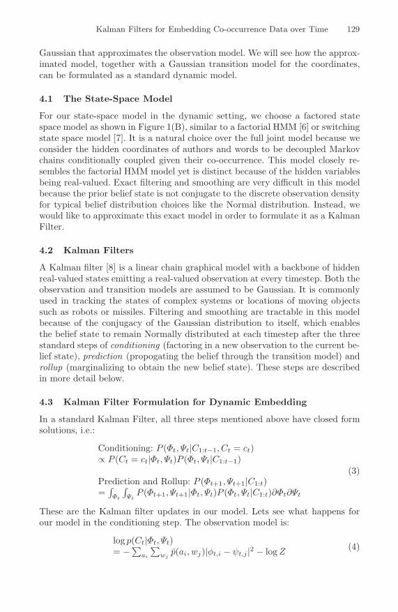
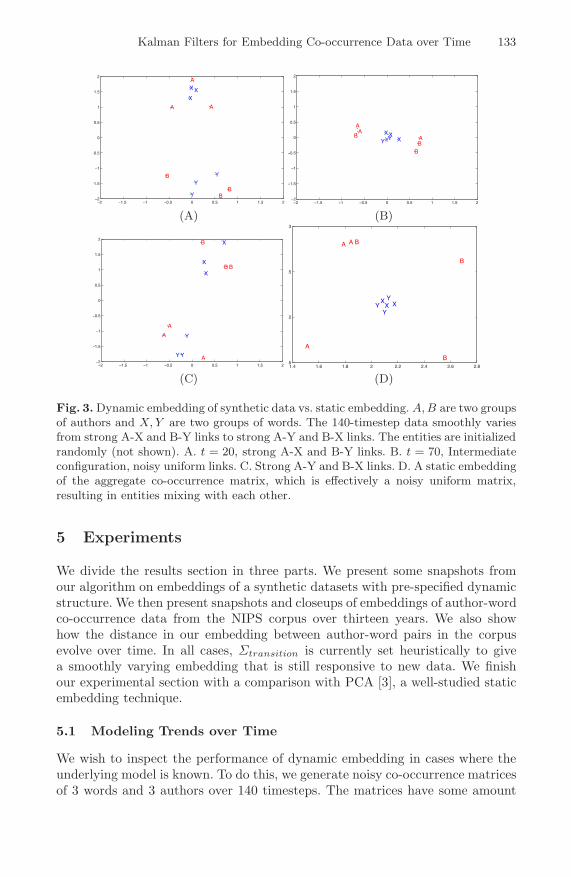
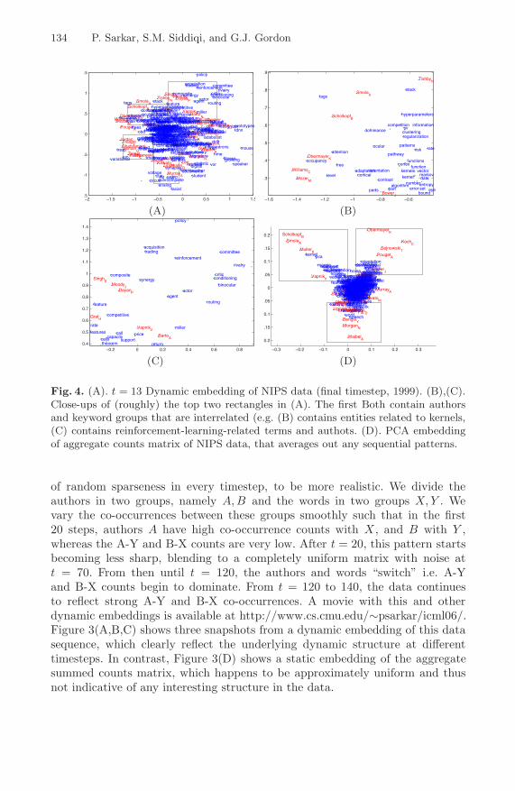
Fig. 4. (A). t = 13 Dynamic embedding of NIPS data (final timestep, 1999). (B),(C).Close-ups of (roughly) the top two rectangles in (A). The first Both contain authorsand keyword groups that are interrelated (e.g. (B) contains entities related to kernels,(C) contains reinforcement-learning-related terms and authots. (D). PCA embeddingof aggregate counts matrix of NIPS data, that averages out any sequential patterns.

of random sparseness in every timestep, to be more realistic. We divide theauthors in two groups, namely A, B and the words in two groups X, Y . Wevary the co-occurrences between these groups smoothly such that in the first20 steps, authors A have high co-occurrence counts with X , and B with Y ,whereas the A-Y and B-X counts are very low. After t = 20, this pattern startsbecoming less sharp, blending to a completely uniform matrix with noise att = 70. From then until t = 120, the authors and words “switch” i.e. A-Yand B-X counts begin to dominate. From t = 120 to 140, the data continuesto reflect strong A-Y and B-X co-occurrences. A movie with this and otherdynamic embeddings is available at http://www.cs.cmu.edu/∼psarkar/icml06/.Figure 3(A,B,C) shows three snapshots from a dynamic embedding of this datasequence, which clearly reflect the underlying dynamic structure at differenttimesteps. In contrast, Figure 3(D) shows a static embedding of the aggregatesummed counts matrix, which happens to be approximately uniform and thusnot indicative of any interesting structure in the data.


5.2 The NIPS Corpus

In this section we shall look at word-author co-occurrence data over thirteen yearsfrom the NIPS proceedings of 1986-1999. We implemented the dynamic Kalmanfilter models on a subset of the NIPS dataset. The NIPS data corpus1 containsco-occurrence count data for 13, 649 words and 2, 037 authors appearing togetherin papers from 1986 to 1999. We partitioned this data into yearly raw count ma-trices using additional information in the dataset, and picked a set of well-knownauthors and meaningful keywords. The experiments shown here are carried out onsmall subsets of authors and words in order to get easily interpretable 2-D plotsfor this paper, however the algorithm scales well to larger sets.

Qualitative Analysis. The resulting embedding has some very interestingproperties. The words on different parts of it define different areas of machinelearning. We also find the corresponding authors in those areas. For exam-ple in figure 4(A) we have presented the embedding of 40 authors and 428words. These are the overall most popular authors, and the words they tendto use.

We can divide the area in the figure in four clear areas, within the rectangles.The top right region magnified in Figure 4(C) has words like reinforcement,agent, actor, policy which clearly are words from the field of reinforcementlearning. We also have authors such as Singh, Dayan and Barto in the same area.Dayan is known to have worked on acquisition and trading which are alsowords in this region. However the very neighboring region on the left belongsto words like kernel, regularization, error and bound. We see some overlapwith that region via the entities support and Vapnik. Also one of the othertwo interesting regions consists of authors Jordan, Hinton, Gharamani Zemel,Tresp. The lowest rectangular region is filled with words and authors like image,segmentation, motion, movement. Notably we find that author Viola is placedvery close to these words and words like document, retrieval,facial. Alsowe have author Murray co-placed with words voltage, circuit, chip, analog,synapse. These are strongly supported by the co-occurrence data and anecdotalevidence.

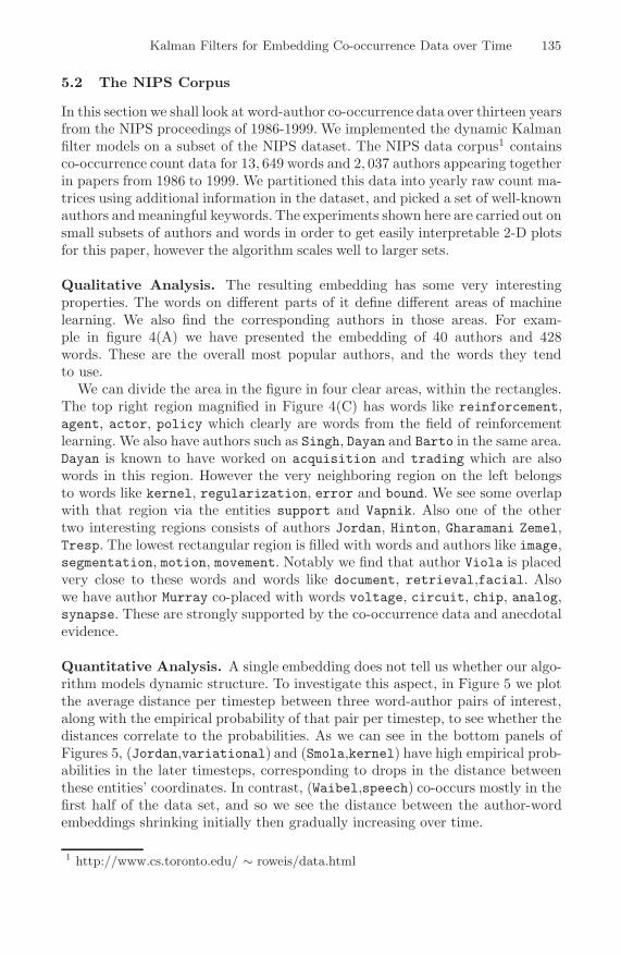
Quantitative Analysis. A single embedding does not tell us whether our algo-rithm models dynamic structure. To investigate this aspect, in Figure 5 we plotthe average distance per timestep between three word-author pairs of interest,along with the empirical probability of that pair per timestep, to see whether thedistances correlate to the probabilities. As we can see in the bottom panels ofFigures 5, (Jordan,variational) and (Smola,kernel) have high empirical prob-abilities in the later timesteps, corresponding to drops in the distance betweenthese entities’ coordinates. In contrast, (Waibel,speech) co-occurs mostly in thefirst half of the data set, and so we see the distance between the author-wordembeddings shrinking initially then gradually increasing over time.

1 http://www.cs.toronto.edu/ ∼ roweis/data.html


0 2 4 6 8 10 12 140

0.5

1

1.5

2

auth

or−

wor

d D

ista

nce

a = Jordan, w = variational

0 2 4 6 8 10 12 140

0.2

0.4

0.6

0.8

1

Timesteps

empi

rical

pro

babi

lity

P(a|w)

0 2 4 6 8 10 12 140

0.5

1

1.5

auth

or−

wor

d D

ista

nce

a = Smola, w = kernel

0 2 4 6 8 10 12 140

0.1

0.2

0.3

0.4

Timesteps

empi

rical

pro

babi

lity

P(a|w)

0 2 4 6 8 10 12 140

0.5

1

1.5

auth

or−

wor

d D

ista

nce

a = Waibel, w = speech

0 2 4 6 8 10 12 140

0.2

0.4

0.6

0.8

Timesteps

empi

rical

pro

babi

lity

P(a|w)

(A) (B) (C)

Fig. 5. Average distance between author-word pairs over time (above), along withcorresponding empirical probabilities (below). A. Jordan and variational. B. Smola andkernel C. Waibel and speech. The graphs on the bottom reflect empirical p(author |word) from the NIPS data which varies inversely over time with the average author-word distance in the embedding shown in the top row, demonstrating the responsivenessof the embeddings to the underlying data.

5.3 Comparison with PCA

An embedding of the aggregate data with PCA is shown in Figure 4(D). Theembedding reflects relationships in the overall data very well, as seen in the threerectangles highlighted. For example, one of them has entities like Scholkopf,Smola, kernel and pca, and the others also have consistent sets of authors andthe keywords they are known to use. However the data fails to capture dynamictrends in the data that our model successfully reflects. For example, Waibeland speech do not co-occur at all in the latter timesteps of the dataset, as isclear from the lower panel of Figure 5(C). However, since the aggregate countsmatrix embedded by static PCA averages out all sequential structure, Waibeland speech are still relatively close in the PCA embedding.

6 Conclusion and Future Work

We have proposed and demonstrated a model for Euclidean embedding of co-occurrence data over time by formulating the problem as a factored state spacemodel, and used an approximation to yield a tractable Kalman filter formu-lation. The resulting model gives us an estimate of the posterior distributionover the coordinates of the entities in latent space. The previous work we areextending addresses this problem only for the single-timestep case, giving onlypoint estimates for the coordinates. Experimental results show that our modelyields interpretable visual results and reflects dynamic trends in the data. Forfuture work we will implement smoothing in the dynamic model to see if it offersimproved results over filtering. We will also obtain quantitative results for themodel on problems such as link prediction in social networks and classificationin word-document embedding.


Acknowledgements

We warmly thank Carlos Guestrin for his guidance. This work was funded inpart by DARPA’s CS2P program under grant number HR0011-006-1-0023. Theopinions and conclusions expressed are the authors’.

References

1. Globerson, A., Chechik, G., Pereira, F., Tishby, N.: Euclidean embedding of co-occurrence data. In: Proc. Eighteenth Annual Conf. on Neural Info. Proc. Systems(NIPS). (2004)

2. Sarkar, P., Moore, A.: Dynamic social network analysis using latent space models.In: Proc. Nineteenth Annual Conf. on Neural Info. Proc. Systems (NIPS). (2005)

3. Berry, M., Dumais, S., Letsche, T.: Computational methods for intelligent informa-tion access. In: Proceedings of Supercomputing. (1995)

4. Breiger, R.L., Boorman, S.A., Arabie, P.: An algorithm for clustering relational datawith applications to social network analysis and comparison with multidimensionalscaling. J. of Math. Psych. 12 (1975) 328–383

5. Raftery, A.E., Handcock, M.S., Hoff, P.D.: Latent space approaches to social networkanalysis. J. Amer. Stat. Assoc. 15 (2002) 460

6. Ghahramani, Z., Jordan, M.I.: Factorial hidden Markov models. In Touretzky, D.S.,Mozer, M.C., Hasselmo, M.E., eds.: Proc. Conf. Advances in Neural InformationProcessing Systems, NIPS. Volume 8., MIT Press (1995) 472–478

7. Ghahramani, Z., Hinton, G.E.: Switching state-space models. Technical report, 6King’s College Road, Toronto M5S 3H5, Canada (1998)

8. Kalman, R.: A new approach to linear filtering and prediction problems. (1960)9. Jordan, M.I., Ghahramani, Z., Jaakkola, T.S., Saul, L.K.: An Introduction to Vari-

ational Methods for Graphical Methods. Machine Learning (1998)

Appendix

In this section we give a detailed description of the derivations.

Derivation of Section 4.4

We compute the KL projection of our observation model (p) to the closestGaussian family (q).

D(p, q) =∫

p ln p −∫

p ln q= −H(p) +

∫(∑

ij pij(φi − ψj)T (φi − ψj))dp + Ep(ln Z)

= −(A + W ) − ln((2π)2(A+W )|Σ|)2

+Ep(∑

ij pij(φi − ψj)T (φi − ψj)) + Ep(ln Z)

(9)

Using equations 5 and 6 we get a lower bound on equation 9.

D(p, q) ≥ −(A + W ) − ln((2π)2(A+W )|Σ|)2

+Ep(∑

ij(pij − pipj)(φi − ψj)T (φi − ψj))

≥ −(A + W ) − ln((2π)2(A+W )|Σ|)2 + Ep(χT Λ̂χ)


We get the expression in equation 8 by parameter matching. Differentiatingthe above equation w.r.t Σ gives us the parameters for the closest Gaussian weproject our distribution into.

Derivation of Section 4.4

Now we derive the approximate observation model using Taylor expansion of theexponentiated distance term of the normalization constant, i.e. e−(φi−ψj)T (φi−ψj)

around parameters ξi, ξj . We define the gradient (∇) and Hessian (H) for ourfunction. The gradient is defined as follows:

∇1(ξi, ξj) = (∂g

∂φi)ξi,ξj = −2e−(ξi−ξj)T (ξi−ξj)(φi − ψj)

∇2(ξi, ξj) = (∂g

∂ψj)ξi,ξj = −∇1(ξi, ξj)

H =

(∂2g

∂ΦTt ∂ΦT

t

∂2g∂ΨT

t ∂Φt

∂2g∂ΦT

t ∂Ψt

∂2g∂ΨT

t ∂ΨTt

)

ξi,ξj

=(

H11 H12H21 H22

)

The second order approximation of e−(φi−ψj)T (φi−ψj) gives

1 + φTi ∇1 + ψT

j ∇2 + 12 [ΦT

t ΨTt ]H(ξi, ξj)[ΦtΨt]

= 1 + 12 [φT

i H11φi + ψTj H21φi + φT

i H12ψj + ψTj H22ψj ]

(10)

Where H(ξi, ξj) is H evaluated at ξi, ξj . For our purpose these values evaluateto the following:

H11 = 2e−(ξi−ξj)T (ξi−ξj)(2(ξi − ξj)(ξi − ξj)T − I)H12 = −H11H21 = −HT

11H22 = H22

(11)

We also define the following symmetric matrix η and Λ for making the derivationssimple. Also here η is 2(A+W ) a dimensional vector and Λ is a 2(A+W ), 2(A+W ) dimensional symmetric matrix. By i we denote author i and by j we indexword j.

ηi = pi

∑j pj∇1(ξi, ξj)

ηj = pj

∑i pi∇2(ξi, ξj)

(12)

Λii = pi

∑j pjH11(ξi, ξj)

Λjj = pj

∑i piH22(ξi, ξj)

Λij = pipjH12(ξi, ξj)(13)


Now using equations (10), (13) and (11) the expectation of the log normalizingconstant under the new distribution becomes:

Ep(∑

ij pipje−(φi−ψj)T (φi−ψj))

= c + Ep[∑

i φTi ηi +

∑j ψT

j ηj ]+12Ep[

∑i φT

i Λiiφi + 2∑

ij φTi Λijψi +

∑j φT

j Λjjφj ]= c + Ep[χT η] + 1

2Ep[χT Λχ]= c + μT η + 1

2Tr((μμT + Σ)Λ)

All terms independent of μ, Σ are combined in the constant term c. Hence theapproximation of D(p, q) comes out to be,

D(p, q) ≈ C − 12 ln|Σ| + tr((μμT + Σ))Λ̃) + λμT η+

λ2 Tr((μμT + Σ)Λ)

A derivative w.r.t Σ and μ yields

Λ = Σ−1 = 2(Λ̃ + λ2 Λ)

η = −λη

which are the required parameters for the Gaussian approximation of the obser-vation model used in the Kalman filter.

Documents

LNCS 4503 - Approximate Kalman Filters for Embedding Author-Word Co-occurrence …airoldi/pub/books/b01... · · 2008-04-14Approximate Kalman Filters for Embedding Author-Word Co-occurrence