Notes on Kalman Filtering

Brian Borchers and Rick Aster

November 7, 2011

Introduction

Data Assimilation is the problem of merging model predictions with actual mea-surements of a system to produce an optimal estimate of the current state ofthe system and/or predictions of the future state of the system. For exam-ple, weather forecasters run massive computational models that predict winds,temperature, etc. As time progresses, it is important to incorporate availableweather observations into the mathematical model. Since these weather obser-vations are noisy, the problem of incorporating the observations into the modelis inherently statistical in nature.

Data Assimilation is becoming a very hot topic in many areas of science, in-cluding atmospheric physics, oceanography, and hydrology. In the next few lec-tures, we’ll introduce Kalman filtering, which is one of the simplest approachesto data assimilation. The Kalman filter was introduced in a 1960 paper by R.E. Kalman.

The Model Of The System

Consider a discrete time dynamical system governed by the equation

xk = Axk−1 +Buk−1 + wk−1. (1)

Here, xk, uk−1, and wk−1 are vectors and the subscripts refer to the time stepsrather than indexing elements of the vectors. The state of the system at timek is given by the vector xk. Deterministic inputs to the system at time k − 1are given by uk−1. Random noise affecting the system at time k − 1 is givenby wk−1. We’ll assume that wk−1 has a multivariate normal distribution withmean 0 and covariance matrix Q.

We’ll obtain a vector of measurements zk at time k, where zk is given by

zk = Hxk + vk. (2)

Here vk represents random noise in the observation zk. We’ll assume that vk isnormally distributed with mean 0 and covariance matrix R.

1

The matrices A, B, H, Q, and R are all assumed to be known, although theKalman filter can be extended to simultaneously estimate these matrices alongwith xk. For now, our goal is to estimate xk and predict xk+1, xk+2, . . ., asaccurately as possible given z1, z2, . . ., zk.

The estimate that we will obtain will come in the form of a multivariatenormal distribution with a specified mean xk and covariance matrix Pk. Wewill want to measure the “tightness” of this multivariate normal distribution.A convenient measure of the tightness of an MVN distribution with covariancematrix C is

trace(C) = C1,1 + C2,2 + . . .+ Cn,n. (3)

trace(C) = V ar(X1) + V ar(X2) + . . .+ V ar(Xn). (4)

Example 1 For example, xk might be a six element vector containing theposition (3 coordinates) and velocity (3 coordinates) of an aircraft at time k.The vector uk−1 might represent control inputs (thrust, elevator, rudder, etc.)to the aircraft at time k− 1, and wk−1 might represent the effects of turbulenceon the aircraft. We may be using a very simple radar to observe the aircraft, sothat we get measurements of the position, z, but not the velocity of the aircraftat each moment in time. These measurements of the aircraft’s position mightalso be noisy.

In many cases, the system that we’re interested in is described by a systemof differential equations in continuous time:

x′(t) = Ax(t) +Bu(t). (5)

We can discretize this system of equations using time steps of length ∆t, to get

x(t+ ∆t) = x(t) + ∆tx′(t). (6)

x(t+ ∆t) = x(t) + ∆t(Ax(t) +Bu(t)). (7)

Letting xk = x(t+ ∆t) and xk−1 = x(t), we get

xk = (I + ∆tA)xk−1 + ∆tBuk−1. (8)

In many practical applications of Kalman filtering the mathematical modelof the system consists of an even more complicated system of partial differentialequations. Such systems are commonly discretized using finite difference orfinite element methods. Rather than diving into the details of the numericalanalysis used in discretizing PDE’s, we will simply assume that our problem hasbeen cast in the form of (1).

The Kalman Filter

We have two sources of information that can help us in estimating the state ofthe system at time k. First, we can use the equations that describe the dynamicsof the system. Substituting wk−1 = 0 into (1), we might reasonably estimate

xk = Axk−1 +Buk−1 (9)

2

A second useful source of information is our observation zk. We might pick xk

so as to minimize ‖zk −Hxk‖. There’s an obvious trade-off between these twomethods of estimating xk. The Kalman filter produces a weighted combina-tion of these two estimates that is optimal in the sense that it minimizes theuncertainty of the resulting estimate.

We’ll begin the estimation process with an initial guess for the state ofthe system at time 0. Since we want to keep track of the uncertainty in ourestimates, we’ll have to specify the uncertainty in our initial guess. We describethis by using a multivariate normal distribution

x0 ∼ N(x0, P0). (10)

In the prediction step, we are given an estimate xk−1 of the state of thesystem at time k − 1, with associated covariance matrix Pk−1. We substitutethe mean value of wk−1 = 0 into (1) to obtain the estimate

x−k = Axk−1 +Buk−1. (11)

The minus superscript is used to distinguish this estimate from the final estimatethat we get after including the observation zk. The covariance of our newestimate is

P−k = Cov(x−k ). (12)

P−k = Cov(Axk−1 +Buk−1 + wk−1). (13)

The Buk−1 term is not random, so its covariance is zero. The covariance ofwk−1 is Q. The covariance of Axk−1 is A Cov(xk−1)AT . Thus

P−k = ACov(xk−1)AT +Q. (14)

P−k = APk−1AT +Q. (15)

We could simply repeat this process for x1, x2, . . .. If no observations of thesystem are available, that would be an appropriate way to estimate the systemstate.

In the update step, we modify the prediction estimate to include the obser-vation.

xk = x−k +Kk(zk −Hx−k ) (16)

xk = (I −KkH)x−k +Kkzk. (17)

Here the factor Kk is called the Kalman gain. It adjusts the relative influenceof zk and x−k . We will soon show that

Kk = P−k HT (HP−k H

T +R)−1 (18)

is optimal in the sense that it minimizes the trace of Pk.The covariance of our updated estimate is

Pk = Cov(xk). (19)

3

Pk = Cov((I −KkH)x−k +Kkzk). (20)

Pk = (I −KkH)P−k (I −KkH)T +KkCov(zk)KTk . (21)

Since Cov(zk) = R,

Pk = (I −KkH)P−k (I −KkH)T +KkRKTk . (22)

This simplifies to

Pk = P−k −KkHP−k − P

−k H

TKTk +Kk(HP−k H

T )KTk +KkRK

Tk . (23)

Pk = P−k −KkHP−k − P

−k H

TKTk +Kk(HP−k H

T +R)KTk . (24)

We want to minimize the trace of Pk. Using vector calculus, it can be shownthat

∂trace(Pk)∂Kk

= −2(HP−k )T + 2Kk(HP−k HT +R). (25)

Setting the derivative equal to 0,

−2(HP−k )T + 2Kk(HP−k HT +R) = 0. (26)

Kk = (HP−k )T (HP−k HT +R)−1. (27)

Kk = P−k HT (HP−k H

T +R)−1. (28)

Using this optimal Kalman gain, Pk simplifies further.

Pk = P−k −KkHP−k − P

−k H

TKTk +Kk(HP−k H

T +R)KTk . (29)

Pk = P−k − P−KH

T (HP−k HT +R)−1HP−k −

P−k HT (P−KH

T (HP−k HT +R)−1))T +

P−KHT (HP−k H

T +R)−1(HP−k HT +R)(P−k H

T (HP−k HT +R)−1)T (30)

Pk = P−k − P−k H

T (HP−k HT +R)−1HP−k (31)

Pk = (I −KkH)P−k . (32)

The algorithm can be summarized as follows. For k = 1, 2, . . .,

1. Let x−k = Axk−1 +Buk−1.

2. Let P−k = APk−1AT +Q.

3. Let Kk = P−k HT (HP−k H

T +R)−1.

4. Let xk = x−k +Kk(zk −Hx−k ).

5. Let Pk = (I −KkH)P−k .

4

In practice, we may not have an observation at every time step. In that case,we can use predictions at each time step and compute updates steps wheneverobservations become available.

Example 2 In this example, we’ll consider a system governed by the secondorder differential equation

y′′(t) + 0.01y′(t) + y(t) = sin(2t) (33)

with the initial conditions y(0) = 0.1, y′(0) = 0.5.We must first use a standard trick to convert this second order ordinary

differential equation into a system of two first order differential equations. Let

x1(t) = y(t) (34)

andx2(t) = y′(t). (35)

The relation between x1(t) and x2(t) is

x′1(t) = x2(t). (36)

Also, (33) becomes

x′2(t) = −x1(t)− 0.01x2(t) + sin(2t). (37)

This system of two first order equations can be written as

x′(t) = Ax(t) +Bu(t) (38)

where

A =[

0 1−1 −0.01

], (39)

B =[

1 00 1

], (40)

and

u(t) =[

0sin(2t)

]. (41)

This system of differential equations will be discretized using (8) with timesteps of ∆t = 0.01. At each time step, the state vector will be randomlyperturbed with N(0, Q), noise, where

Q =[

0.0005 0.00.0 0.0005

]. (42)

We will observe x1(t) once per second (every 100 time steps.) Thus

H =[

1 0]. (43)

5

Our observations will have a variance of 0.0005.For the initial conditions we will begin with the estimate

x0 =[

00

](44)

and covariance

P0 =[

0.5 0.00.0 0.5

]. (45)

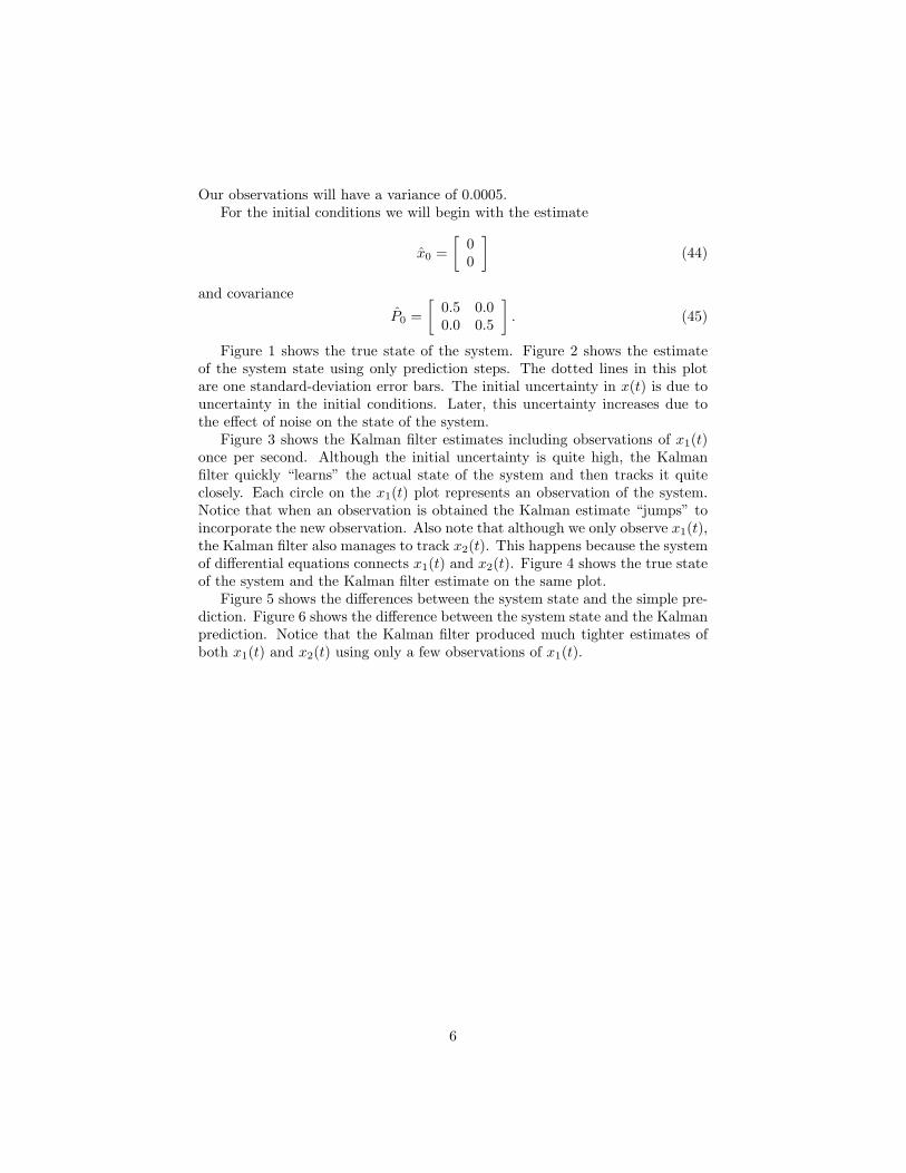
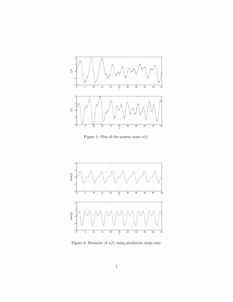
Figure 1 shows the true state of the system. Figure 2 shows the estimateof the system state using only prediction steps. The dotted lines in this plotare one standard-deviation error bars. The initial uncertainty in x(t) is due touncertainty in the initial conditions. Later, this uncertainty increases due tothe effect of noise on the state of the system.

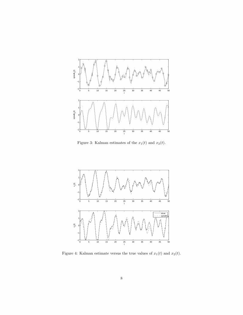
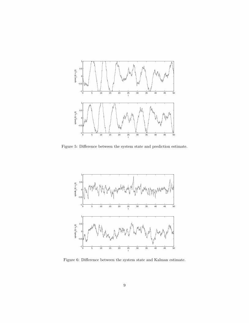
Figure 3 shows the Kalman filter estimates including observations of x1(t)once per second. Although the initial uncertainty is quite high, the Kalmanfilter quickly “learns” the actual state of the system and then tracks it quiteclosely. Each circle on the x1(t) plot represents an observation of the system.Notice that when an observation is obtained the Kalman estimate “jumps” toincorporate the new observation. Also note that although we only observe x1(t),the Kalman filter also manages to track x2(t). This happens because the systemof differential equations connects x1(t) and x2(t). Figure 4 shows the true stateof the system and the Kalman filter estimate on the same plot.

Figure 5 shows the differences between the system state and the simple pre-diction. Figure 6 shows the difference between the system state and the Kalmanprediction. Notice that the Kalman filter produced much tighter estimates ofboth x1(t) and x2(t) using only a few observations of x1(t).

6

0 5 10 15 20 25 30 35 40 45 50−2

−1

0

1

2

t

x 1(t)

0 5 10 15 20 25 30 35 40 45 50−2

−1

0

1

2

t

x 2(t)

Figure 1: Plot of the system state x(t).

0 5 10 15 20 25 30 35 40 45 50−2

−1

0

1

2

t

xpre

d 1(t)

0 5 10 15 20 25 30 35 40 45 50−2

−1

0

1

2

t

xpre

d 2(t)

Figure 2: Estimate of x(t) using prediction steps only.

7

0 5 10 15 20 25 30 35 40 45 50−2

−1

0

1

2

t

xpre

dk1(t

)

0 5 10 15 20 25 30 35 40 45 50−2

−1

0

1

2

t

xpre

dk2(t

)

Figure 3: Kalman estimates of the x1(t) and x2(t).

0 5 10 15 20 25 30 35 40 45 50−2

−1

0

1

2

t

x 1(t)

0 5 10 15 20 25 30 35 40 45 50−2

−1

0

1

2

t

x 2(t)

xtruexpredk

Figure 4: Kalman estimate versus the true values of x1(t) and x2(t).

8

0 5 10 15 20 25 30 35 40 45 50−1

−0.5

0

0.5

1

t

xpre

d 1(t)−

x 1(t)

0 5 10 15 20 25 30 35 40 45 50−1

−0.5

0

0.5

1

t

xpre

d 2(t)−

x 2(t)

Figure 5: Difference between the system state and prediction estimate.

0 5 10 15 20 25 30 35 40 45 50−1

−0.5

0

0.5

1

t

xpre

dk1(t

)−x 1(t

)

0 5 10 15 20 25 30 35 40 45 50−1

−0.5

0

0.5

1

t

xpre

dk2(t

)−x 2(t

)

Figure 6: Difference between the system state and Kalman estimate.

9

The Extended Kalman Filter

The Extended Kalman Filter (EKF) extends the Kalman filtering concept toproblems with nonlinear dynamics. Our new equation for the time evolution ofthe system state will be of the form

xk = f(xk−1, uk−1, wk−1) (46)

where wk−1 is a random perturbation of the system. This time, we’ll assumethat wk−1 has a multivariate normal distribution with mean 0 and covariancematrix Qk−1. That is, the covariance is allowed to be time dependent.

Our new measurement model will be

zk = h(xk, vk) (47)

where vk is a multivariate normal N(0, Rk) noise vector.The prediction step is a straight forward generalization of what we have

previously done in the Kalman filter.

x−k = f(xk−1, uk−1, 0). (48)

We’ll also introduce a new notation for the predicted observation

z−k = h(x−k , 0). (49)

In general, for a nonlinear function f , x−k will not have a multivariate normaldistribution. However, we can reasonably hope that f(x, u, w) will be approxi-mately linear for relatively small changes in x and w, so that x−k will be at leastapproximately normally distributed.

We linearize f(x, u, w) around (xk−1, uk−1, 0) as

f(x, u, w) = f(xk−1, uk−1, 0) +Ak−1(x− xk−1) +Wk−1(w − 0) (50)

where A and W are matrices of partial derivatives of f with respect to x and w.Note that since uk−1 is assumed to be known exactly, we don’t need to linearizein the u variable. The entries in Ak−1 and Wk−1 are given by

Ai,j,k−1 =∂fi(xk−1, uk−1, 0)

∂xj. (51)

Wi,j,k−1 =∂fi(xk−1, uk−1, 0)

∂wj. (52)

Using this linearization, we end up with an approximate covariance matrix forx−k ,

P−k = Ak−1Pk−1ATk−1 +Wk−1Qk−1W

Tk−1. (53)

Similarly, we can linearize h(). Let

Hi,j,k =∂hi(x−k , 0)

∂xj. (54)

10

Vi,j,k =∂hi(x−k , 0)

∂vj. (55)

Now, lete−xk

= xk − x−k (56)

ande−zk

= zk − z−k . (57)

We don’t actually know xk, but we do expect xk− x−k to be relatively small.Thus we can use our linearization of f() to derive an approximation for e−xk

.

e−xk= f(xk−1, uk−1, wk−1)− f(xk−1, uk−1, 0). (58)

By the linearization,

e−xk≈ Ak−1(xk−1 − xk−1) + εk (59)

where εk accounts for the effect of the random wk−1. The distribution of εk isN(0,Wk−1Qk−1W

Tk−1). Similarly,

e−zk= h(xk, vk)− h(x−k , 0). (60)

By the linearization this is approximately

e−zk≈ He−xk

+ ηk (61)

where ηk has an N(0, VkRkVTk ) distribution.

Ideally, we could update x−k to get xk by

xk = x−k + e−xk. (62)

Of course, we don’t know e−xk, but we can estimate it. Let

exk= Kk(zk − z−k ) (63)

where Kk is a Kalman gain factor to be determined. Then let

xk = x−k + exk. (64)

By a derivation similar to our earlier derivation of the optimal Kalman gain forthe linear Kalman filter, it can be shown that the optimal Kalman gain for theEKF is

Kk = P−k HTk (HkP

−k H

Tk + VkRkV

Tk )−1. (65)

Using this optimal Kalman gain, the covariance matrix for the updated estimatexk is

Pk = (I −KkHk)P−k . (66)

11

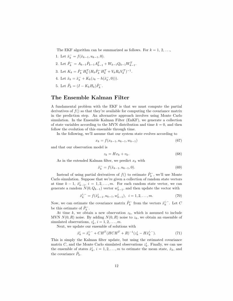
The EKF algorithm can be summarized as follows. For k = 1, 2, . . .,

1. Let x−k = f(xk−1, uk−1, 0).

2. Let P−k = Ak−1Pk−1ATk−1 +Wk−1Qk−1W

Tk−1.

3. Let Kk = P−k HTk (HkP

−k H

Tk + VkRkV

Tk )−1.

4. Let xk = x−k +Kk(zk − h(x−k , 0))).

5. Let Pk = (I −KkHk)P−k .

The Ensemble Kalman Filter

A fundamental problem with the EKF is that we must compute the partialderivatives of f() so that they’re available for computing the covariance matrixin the prediction step. An alternative approach involves using Monte Carlosimulation. In the Ensemble Kalman Filter (EnKF), we generate a collectionof state variables according to the MVN distribution and time k = 0, and thenfollow the evolution of this ensemble through time.

In the following, we’ll assume that our system state evolves according to

xk = f(xk−1, uk−1, wk−1) (67)

and that our observation model is

zk = Hxk + vk. (68)

As in the extended Kalman filter, we predict xk with

x−k = f(xk−1, uk−1, 0). (69)

Instead of using partial derivatives of f() to estimate P−k , we’ll use MonteCarlo simulation. Suppose that we’re given a collection of random state vectorsat time k − 1, xi

k−1, i = 1, 2, . . . ,m. For each random state vector, we cangenerate a random N(0, Qk−1) vector wi

k−1, and then update the vector with

xi,−k = f(xi

k−1, uk−1, wik−1), i = 1, 2, . . . ,m. (70)

Now, we can estimate the covariance matrix P−k from the vectors xi,−k . Let C

be this estimate of P−k .At time k, we obtain a new observation zk, which is assumed to include

MVN N(0, R) noise. By adding N(0, R) noise to zk, we obtain an ensemble ofsimulated observations, zi

k, i = 1, 2, . . . ,m.Next, we update our ensemble of solutions with

xik = xi,−

k + CHT (HCHT +R)−1(zik −Hx

i,−k ). (71)

This is simply the Kalman filter update, but using the estimated covariancematrix C, and the Monte Carlo simulated observations zi

k. Finally, we can usethe ensemble of states xi

k, i = 1, 2, . . . ,m to estimate the mean state, xk, andthe covariance Pk.

12