Data Assimilation by Morphing Fast Fourier TransformEnsemble Kalman Filter for Precipitation Forecasts using

Radar Images1

Jan Mandel2, Jonathan D. Beezley2, Krystof Eben3, Pavel Jurus3,Volodymyr Y. Kondratenko2, and Jaroslav Resler3

April 2010

Abstract

The FFT EnKF takes advantage of the theory of random fields and the FFT toprovide a good and cheap approximation of the state covariance with a very smallensemble. The method and predecessor components are explained and the method isextended to the case of observations given on a rectangular subdomain, suitable forassimilation of regional radar images into a weather model.

Contents

1 Introduction 1

2 Background 32.1 Sequential data assimilation . . . . . . . . . . . . . . . . . . . . . . . . . . . . . . . . 32.2 The EnKF . . . . . . . . . . . . . . . . . . . . . . . . . . . . . . . . . . . . . . . . . . 42.3 Smooth random functions by FFT . . . . . . . . . . . . . . . . . . . . . . . . . . . . 62.4 Morphing EnKF . . . . . . . . . . . . . . . . . . . . . . . . . . . . . . . . . . . . . . 7

3 FFT EnKF 83.1 The basic algorithm . . . . . . . . . . . . . . . . . . . . . . . . . . . . . . . . . . . . 83.2 Multiple variables . . . . . . . . . . . . . . . . . . . . . . . . . . . . . . . . . . . . . . 103.3 Observations on a subdomain . . . . . . . . . . . . . . . . . . . . . . . . . . . . . . . 11

4 The complete method 12

1 Introduction

Incorporating new data into computations in progress is a well-known problem in weather forecast-ing, and techniques to incorporate new data by sequential Bayesian estimation are known as dataassimilation [12]. The basic framework is the discrete time state-space model in its most generalform is an application of the Bayesian update problem. In the Gaussian case, direct application of

1This research was partially supported by the National Science Foundation under the grants CNS-0719641 andATM-0835579.

2Center for Computational Mathematics and Department for Mathematical and Statistical Sciences, Universityof Colorado Denver, Denver CO 80217-3364, USA.

3Institute of Computer Science, Academy of Sciences of the Czech Republic, Pod Vodarenskou vezi 2, 182 07Prague 8, Czech Republic.

1

the Bayes theorem with assumed state covariance becomes the classical optimal statistical inter-polation. A more general method, the Kalman filter evolves the state covariance by the dynamicsof the system, but it is not suitable for high-dimensional problems, due to the need to maintainthe covariance matrix. The ensemble Kalman filter (EnKF) [7] is a Monte-Carlo implementationof the Kalman filter, which replaces the state covariance by sample covariance of an ensemble ofsimulations. The EnKF has become quite popular because it allows an implementation withoutany change to the model; the model only needs to be capable of exporting its state and restartingfrom the state modified by the EnKF. However, there are two main drawbacks to the EnKF.

First, a reasonable approximation of the state covariance by the sample covariance requiresa large ensemble, easily many hundreds [7]. Techniques to improve the approximation of thestate distribution by the ensemble include non-random selection of the initial ensemble such asLyapunov vectors or bred vectors [12], and localization techniques such as covariance tapering [8],the Ensemble Adjustment Kalman Filter [2], and the Local Ensemble Transform Kalman Filter[10]. This paper builds on the Fast Fourier Transform (FFT) EnKF, introduced in [15, 17]. TheFFT EnKF takes advantage of the fact that the state is approximately a stationary random field,that is, the covariance between two points is mainly a function of their distance vector. Thenthe multiplication of the covariance matrix and a vector is approximately a convolution, so thecovariance matrix in the frequency domain can be well aproximated by its diagonal. This resultsin a good approximation of the covariance for very small ensembles with no need for tapering, aswell as an efficient implementation of the EnKF formulas by the FFT. It should be noted that therelated Fourier Domain Kalman filter (FDKF) [5] is something else, although it also uses a diagonalcovariance matrix in the frequency domain. The FDKF is the Kalman filter used in each Fouriermode separately, and an ensemble in the FDKF context consists of independent relalizations forthe purpose of post-processing only.

Second, although the EnKF can be and is widely used for quite general probability distri-butions, the EnKF still assumes that the probability distributions are Gaussian, otherwise theimplementation of the Bayes theorem is no longer valid, and the EnKF performace deteriorates.In the Gaussian case, it can be proved that in the large ensemble limit, the ensemble generatedby the EnKF converges to a sample from the filtering distribution computed by the Kalman filter[18]. Combinations of the EnKF and a particle filter for the non-Gaussian case also exist [14].One particular case where strongly non-Gaussian distributions occur are nonlinear systems withsharp coherent moving features, such as weather fronts, firelines, and epidemic waves. In thesecases, the distribution of the position of the coherent features may well be close to Gaussian butthe distribution of the values of the physical variables at any given point is not. This paper usestechniques borrowed from image processing that can be used to transform the state to the so-called morphing representation, which contains both amplitude and position information and ithas a distribution much closer to Gaussian. Then, EnKF techniques can be succesfully used on themorphing representation. [4, 15, 16, 17].

In this paper, we provide a more complete description, motivation, and investigation of theproperties of the FFT EnKF than it was possible in the short conference papers [15, 17]. Inaddition, in [15, 17], the FFT EnKF was limited to the case when the observation consists of onestate variable over the whole physical domain, such as the heat flux from a wildfire, or the numberof infected individuals per unit area in an epidemic simulation. Here, we extend the FFT EnKFto the case when the values of the state variable are observed on a rectangle, which is the caseof radar observations over an area of interest, while the weather simulation executes over a larger

2

domain. We also provide a new and more complete discussion of the crosscovariances, i.e., how theinnovation in the observed variable affects other model variables, which was mentioned in [15, 17]only in passing.

The FFT EnKF method is combined with a new version of the Morphing EnKF [4] on asubdomain, resulting in a method suitable for assimilation of regional radar images into a weathermodel.

2 Background

2.1 Sequential data assimilation

In sequential statistical estimation, the modeled quantity is the probability distribution of thesimulation state. The model is advanced in time until an analysis time. The distribution ofthe system state before, now called the prior or the forecast distribution, and the data likelihoodare now combined to give the new system state distribution, called the posterior or the analysisdistribution. This step is called Bayesian update or analysis step. This completes one analysiscycle, and the model is then advanced until the next analysis time.

In the Bayesian update, the probability density p (u) of the system state u before the update(the prior) and the probability density p (d|u) of the the data d given the value of the system stateu (the data likelihood) are combined to give the new probability density pa (u) of the system stateu with the data incorporated (the posterior) from the Bayes theorem,

pa (u) ∝ p (d|u) p (u) . (1)

where ∝ means proportional. Equation (1) determines the posterior density p (u) completely,because

∫pa (u) du = 1.

Here, we consider the case of linear observation operator H: given system state u, the data value,d, would be Hu if the model and the data were without any errors. Of course, in general, data aregiven such that d 6= Hu, so the discrepancies are modeled by the data likelihood p (d|u). Assumethat the prior has normal distribution with mean µ and covariance Q, and the data likelihood isGaussian with mean Hu and covariance R, that is,

p (u) ∝ exp

(−1

2(u− µ)TQ−1 (u− µ)

), p (d|u) ∝ exp

(−1

2(d−Hu)TR−1 (d−Hu)

).

It can be shown by algebraic manipulations ([1], see also [3, p. 10]) that the posterior distributionis also Gaussian,

pa (u) ∝ exp

(−1

2(u− µa)T (Qa)−1 (u− µa)

),

where the posterior mean µa and covariance Qa are given by the update formulas

µa = µ+K (d−Hu) , Qa = (I −KH)Q, (2)

andK = QHT

(HQHT +R

)−1(3)

is called Kalman gain.

3

When the prior covariance Q is assumed to be known (that is, it is determined by expertjudgement of the modeler), the Bayesian update (2) is known as optimal statistical interpolation.The Kalman filter [11] advances the state covariance by the model explicitly, assuming that themodel is linear. Techniques such as the extended Kalman filter, which advances the state covarianceby a linearization of the model, were developed to treat nonlinear systems. Although Kalman filterand its variants were succesfully used in many applications, they need to store and manipulate thecovariance matrix of the state, which makes them usuitable for high-dimensional systems.

Other, different data assimilation methods were developed for high-dimensional and nonlinearsystem, such as variational data data assimilation (3DVAR and 4DVAR) [12]. These methodsproceed by adjusting the initial conditions (3DVAR) as well as the state at various times in thepast (4DVAR) and they require an additional code, consistent with the model, to implement theso-called adjoint model, which goes back in time to make the adjustment possible.

2.2 The EnKF

The EnKF is a Monte-Carlo implementation of the KF. The EnKF advances an ensemble of inde-pendent simulations [uk] = [u1, . . . , uN ] in time. The ensemble [uk] approximates the probabilitydistribution of the model state u, which is a column vector in Rn. In the analysis step, the ensemble[uk], now called the forecast ensemble, is combined with the data by the EnKF formulas [7, p. 41]

uak = uk +QNHT(HQNH

T +R)−1 (

d+ ek −Hufk), k = 1, . . . , N, (4)

to yield the analysis ensemble [uak]. Here, QN is an approximation of the covariance Q of the modelstate u, and ek is sampled from N (0, R). This completes the analysis cycle, and the ensemble isthen advanced by the simulations in time again.

When QN is the ensemble covariance, the EnKF formulation (4) does not take advantage ofany special structure of the model. Efficient evaluation of the analysis formula (4) is then madepossible by representing the n-by-n sample covariance matrix by an n-by-N matrix E,

QN =1

N − 1

N∑k=1

(Xk −X

) (Xk −X

)T=

1

N − 1EET, (5)

E =[X1 −X, . . . ,XN −X

],

X =1

N

N∑k=1

X.

Efficient schemes for computing with the matrix E only are then possible, and the matrix QN isnever formed explicitly. The method in [16, eq. (15)] is suitable in the case when R has a sparseinverse and it is based on the QR decomposition of E. The procedure in [7, Ch. 14] requiresapproximating R by the sample covariance of the data perturbations ek. This method works for ageneral R, but it requires a more expensive SVD instead of QR decomposition, and the inversiono f the singular matrix in (4) needs special care.

The sample covariance QN , however, is generally a poor approximation on the true state co-variance. It is expected that the state covariance has small or zero entries between variables thatcorrespond to points distant in space, since the small variation in one place should affect places far

4

(a) (b)

(c) (d)

(e) (f)

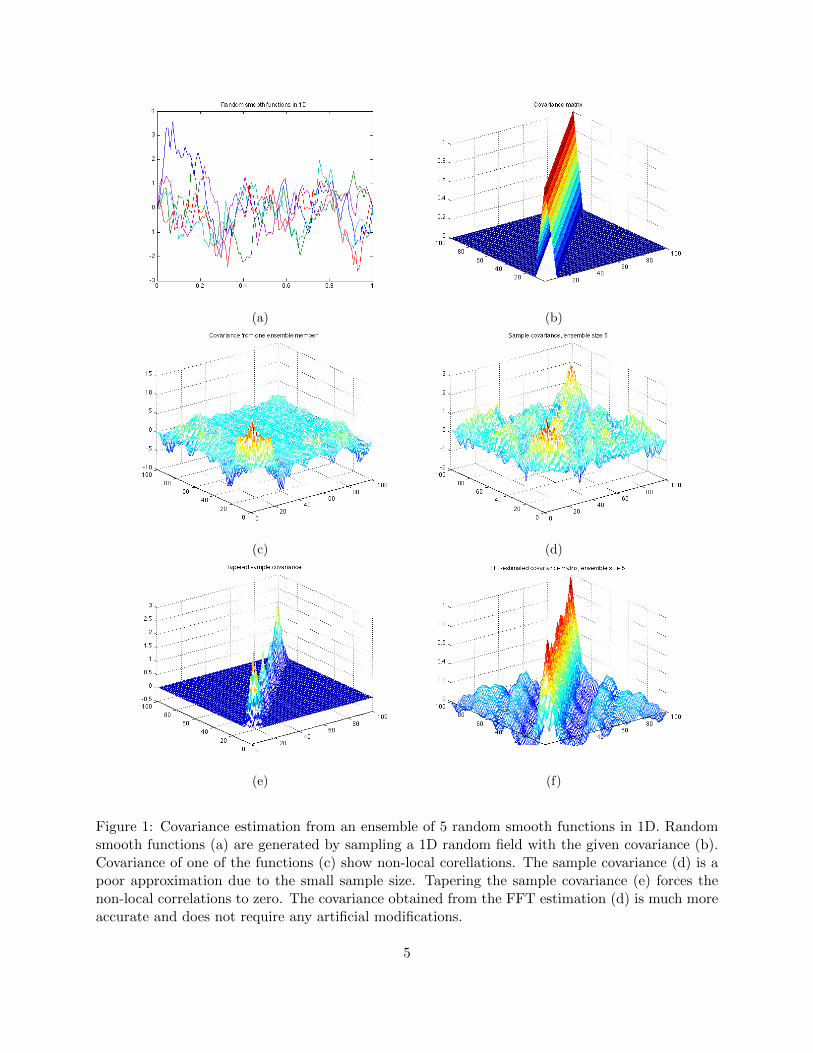
Figure 1: Covariance estimation from an ensemble of 5 random smooth functions in 1D. Randomsmooth functions (a) are generated by sampling a 1D random field with the given covariance (b).Covariance of one of the functions (c) show non-local corellations. The sample covariance (d) is apoor approximation due to the small sample size. Tapering the sample covariance (e) forces thenon-local correlations to zero. The covariance obtained from the FFT estimation (d) is much moreaccurate and does not require any artificial modifications.

5

away. This is also a common assumption in the statistical theory of random fields [6]; the covari-ance of random smooth functions drops off with the distance from the diagonal. However, QN isthe sum of N rank one matrices, with N n. In a rank-one matrix, all columns are proportionalto each other and all rows are proportional to each other, thus having larger entries only closeto the diagonal is not possible (Figure 1c). The sample covariance is the sum of a small numberof rank-one matrices and the same conclusion applies (Figure 1d). Therefore, it was proposed tomodify the sample covariance by multiplication entry-by-entry with a given tapering matrix T toforce the long-range covariances to zero (Figure 1e). That is, the tapered covariance matrix is theSchur product

QN = QN · T, (QN )ij = (QN )ij Tij . (6)

It is known that if T is positive definite then the tapered covariance matrix is at least positivesemidefinite.

Tapering improves the accuracy of the approximate covariance for small ensembles [8], but itmakes the implementation of (4) much more expensive: the sample covariance matrix can no longerbe efficiently represented as the product of two small dense matrices as in (5), but it needs to bemanipulated as a large, albeit sparse, matrix, requiring much more sophisticated and expensivesparse linear algebra.

In general, the state has more than one variable. The state u, the state covariance Q, and theobservation matrix H then have the block form

u =

u(1)

...

u(n)

, Q =

Q(11) · · · Q(1M)

.... . .

...

Q(M1) · · · Q(MM)

, H =[H(1) · · · H(M)

], (7)

with one block per variable. The EnKF analysis formulas (4) with the sample covariance (5) arecompletely oblivious to this structure of the state. However, the choice of the initial ensemble needsto respect it.

2.3 Smooth random functions by FFT

Suppose vk is an orthonormal sequence in a Hilbert space H. Then one can construct a Gaussianrandom element in H,

U =∑∞

k=1ukd1/2k θk

where the constant coefficients dk satisfy

dk ≥ 0,∑∞

k=1dk <∞,

and θk ∼ N (0, 1) are independent. Then E (U) = 0 and the covariance C of U is given by

〈u,Cv〉 = E (〈U, u〉 〈U, v〉)

= E(⟨∑∞

k=1ukd1/2k θk, u

⟩⟨∑∞k=1ukd

1/2k θk, v

⟩)=∑∞

k=1dk 〈uk, u〉 〈uk, v〉 ,

soC =

∑∞k=1dkuku

Tk

6

and dk are the eigenvalues of C.When H is a space of functions u (w), we get the covariance function

C(w,w′

)=∑∞

k=1dkuk (w)uk(w′).

When uk are smooth functions, such as trigonometric functions, U is a smooth random function.Thefaster the coefficients dk decay, the smoother the random function is. For the sin functions and arectangle, we have

U (x, y) =∞∑k=1

∞∑`=1

d1/2k` sin

(xakπ)

sin(yb`π)θk`,

with the covariance function

C((x, y) ,

(x′, y′

))=∞∑k=1

∞∑`=1

dk` sin(xakπ)

sin(yb`π)

sin

(x′

akπ

)sin

(y′

b`π

).

Choose dk` = λ−αk` , where λk` are eigenvalues of the Laplace operator. Then

U (x, y) =∞∑k=1

∞∑`=1

((kπ

a

)2

+

(`π

b

)2)−α/2

sin(xakπ)

sin(yb`π)θk`

and the covariance of the random field U is

C((x, y) ,

(x′, y′

))= E

(U (x, y)U

(x′, u′

))=

∞∑k=1

∞∑`=1

((kπ

a

)2

+

(`π

b

)2)−α/2

sin(xakπ)

sin(yb`π)

sin

(x′

akπ

)sin

(y′

b`π

).

The use of the Green’s function (that is, the inverse) of the Laplace equation as covariance wassuggested earlier in [13].

2.4 Morphing EnKF

Given an initial state u as in (7), the initial ensemble in the morphing EnKF [4, 16] is given by

u(i)k =

(u(i)N+1 + r

(i)k

) (I + Tk) , k = 1, . . . , N, i = 1, . . . ,M, (8)

where denotes composition of mappings, uN+1 = u is considered an additional member of the

ensemble, called the reference member, r(i)k are random smooth functions on Ω, and Tk are random

smooth mappings Tk : Ω→ Ω. Thus, the initial ensemble varies both in amplitude and in position,and the change in position is the same for all variables.

The case considered in EnKF is when the data d is a complete observation of one of the variables,u(1). The data d and the first blocks of all members u1, . . . , uN are then registered against the firstblock of uN+1 by

d ≈ u(1)N+1 (I + T0) , T0 ≈ 0, ∇T0 ≈ 0.

u(1)k ≈ u

(1)N+1 (I + Tk) , Tk ≈ 0, ∇Tk ≈ 0, k = 1, . . . , N, (9)

7

where Tk : Ω→ Ω, k = 0, . . . , N are called registration mappings. The registration mappings Tk arefound by multilevel optimization [3, 4, 9]. The morphing transform maps each ensemble memberuk into the extended state vector

uk 7→ uk = MuN+1 (uk) =(Tk, r

(1)k , . . . , r

(M)k

), (10)

called morphing representation, where

r(j)k = u

(j)k (I + Tk)

−1 − u(j)N+1, k = 0, . . . , N, (11)

are called registration residuals. Note that when u(1)k = u

(1)N+1 (I + Tk) in (9), then r

(j)k = 0; this

happens when all differences between u(1)k and u

(1)N+1 are resolved by position changes. See [4] for

an explantion and motivation of the particular form (11) of the registration residual. Likewise, thedata is mapped into the extended data vector, given by

d 7→ d =(T0, r

(1)0

).

and the observation matrix becomes(T, r(1), . . . , r(M)

)7→(T, r(1)

).

The EnKF is then applied to the transformed ensemble [u1, . . . , uN ], giving the transformedanalysis ensemble [ua1, . . . , u

aN ] and the the new transformed reference member is given by

uaN+1 =1

N

N∑k=1

uak. (12)

The analysis ensemble ua1, . . . , uaN+1 including the new reference member is then obtained by the

inverse morphing transform, defined by

ua,(i)k = M−1uN+1

(uak) =(u(i)N+1 + r

a,(i)k

) (I + T ak ) , k = 1, . . . , N + 1, i = 1, . . . ,M, (13)

similarly as in (8). The analysis ensemble is then advanced by N + 1 independent simulations andthe analysis cycle repeats.

3 FFT EnKF

We explain the FFT EnKF in the 1D case; higher-dimensional cases are exactly the same.

3.1 The basic algorithm

Consider first the case when the model state consists of one variable only. Denote by u (xi),i = 1, . . . , n the entry of vector u corresponding to node xi. If the random field u is stationary,then the covariance matrix satisfies Q (xi, xj) = c (xi − xj) for some covariance function c, andmultiplication by Q is the convolution

v (xi) =

n∑j=1

Q (xi, xj)u (xj) =

n∑j=1

u (xj) c (xi − xj) , i = 1, . . . , n.

8

In the frequency domain, convolution becomes entry-by-entry multiplication of vectors, that is,the multiplication by a diagonal matrix. This is easy to verify for the complex FFT and circularconvolution; however, here we use the real discrete Fourier transform (DFT), either sine or cosine,and convolution with the vectors extended by zero. Then the relation between convolution andentry-by-entry multiplication in the frequency domain is more complicated [19].

We assume that the random field is approximately stationary, so we can neglect the off-diagonalterms of the covariance matrix in the frequency domain, which leads to the the following FFT EnKFmethod. First apply FFT to each member to obtain

uk = Fuk.

Similarly, we denote by the DFT of other quantities. For an n by n matrix M , the correspondingmatrix in the frequency domain is

M = FMF−1,

so thatu = Mv ⇔ u = Mv. (14)

Note that, with a suitable scaling, the DFT is unitary, F ∗F = I and

F ∗ = F−1, (15)

where ∗ denotes conjugate transpose. This is true for the real DFT (sine and cosine) as well.Let uik be the entries of the column vector uk. Using (15), we have the sample covariance in

the frequency domain

QN = FQNF−1 =

1

N − 1

N∑k=1

F (uk − u) (uk − u)T F ∗ (16)

=1

N − 1

N∑k=1

(uk − u

)(uk − u

),

where

u =1

N

N∑k=1

uk,

so the entries of QN are

QNij =1

N − 1

N∑k=1

(uik − ui

)(ujk − uj

), where ui =

1

N

N∑k=1

uik. (17)

We approximate the forecast covariance matrix in the frequency domain by the diagonal matrixC with the diagonal entries given by

ci = QNii =1

N − 1

N∑k=1

∣∣∣uik − ui∣∣∣2 . (18)

The resulting approximation C = F−1CF of the covariance of u tends to be a much betterapproximation than the sample covariance for a small number of ensemble members N (Figure 1f).

9

Multiplication of a vector u by the diagonal matrix C is the same as entry-by-entry multiplica-tion by the vector c = [ci]:

Cu = c • u, (c • u)i = ciui. (19)

Now assume that the observation function H = I, that is, the whole state u is observed. By (14),the evaluation of the EnKF formula (4) in the frequency domain, with the spectral approximationC in the place of QN , becomes

uak = Fuk + FCF−1(FCF−1 + FRF−1

)−1 (Fd+ Fek − Fufk

), (20)

which is simply

uak = uk + C(C + R

)−1 (d+ ek − ufk

), (21)

Further assume that the data error covariance R is such R, and denote by r the diagonal of R. Forexample, when the data error is identical and independent at the mesh points (i.e., white noise),then R is the multiple of identity. A more general diagonal R can be used to model smooth dataerror (Section 2.3). Then, (21) becomes

uak = uk +c

c+ r•(d+ ek − ufk

). (22)

where the operations on vectors are performed entry by entry. The analysis ensemble is obtainedby inverse FFT at the end,

uak = F−1uak.

The FFT EnKF as described here used the sine DFT, which results in zero changes to the stateon the boundary.

In the rest of this section, we describe several variations and extensions of this basic algorithm.

3.2 Multiple variables

Consider the state with multiple variables and the covariance and the observation matrix in theblock form (7). Assume that the first variable is observed, so

H = [I, 0, . . . , 0] .

Then

QNHT =

Q(11) · · · Q(1M)

.... . .

...

Q(M1) · · · Q(MM)

I

...0

=

Q(11)

...

Q(M1)

,

HQNHT = [I, 0, . . . , 0]

Q(11)

...

Q(M1)

= Q(11),

10

and (4) becomes

uak = uk +QNHT(HQNH

T +R)−1 (

d+ ek −Hufk), (23) u

(1),ak...

u(M),ak

=

u(1)k...

u(M)k

+

Q(11)N...

Q(M1)N

(Q(11)N +R

)−1 (d+ ek − u

(1)k

). (24)

In the case when all variables in the state u are based on the same nodes in space and sothe blocks have the same dimension, one can proceed just as in Section 3.1 and approximate thecovariances Q(j1) by their diagonals in the frequency domain. Then, (24) becomes

u(j),ak = u

(j)k +

c(j1)

c(11) + r•(d+ ek − uk

), (25)

where

c(j1)i =

1

N − 1

N∑k=1

(u(j)ik − u

(j)i

)(u(1)ik − u

(1)i

), u

(`)i =

1

N

N∑k=1

u(`)ik . (26)

Note that we are using real DFT, so the complex conjugate in (26) can be dropped.

In the general case, however, the covariance matrices Q(j1)N are rectangular. Fortunately, one

can use FFT with approximation by the diagonal in the frequency space for the efficient evaluationthe inverse in (24) only, while using some other approximation Q(j1)of the covariances Q(j1), whichgives u

(1),ak...

u(M),ak

=

u(1)k...

u(M)k

+

Q(11)

...

Q(M1)

F−1( 1

c(11) + r•(Fd+ Fek − Fu

(1)k

)), (27)

where the operations on vectors are again entry by entry.Possible approximate covariance matrices include the sample covariance, a suitably tapered

sample covariance, and matrices obtained by dropping selected entries of the sample covariance inthe frequency domain. Because the approximate covariances Q(j1) are not involved in a matrixinversion, they do not need to be diagonal in the frequency domain.

3.3 Observations on a subdomain

We now modify the method from Section 3.1 to the case when the observations are given as thevalues of one variable on a subdomain (an interval in 1D, a rectangle in 2D), rather than on thewhole domain, and the observations are based on the same nodes as the state. Then,

H = [P, 0, . . . , 0] , (28)

where P is a zero-one matrix such that multiplication Px selects the values of a vector x in theobserved subdomain. Substituting this observation matrix into (23), (24) becomes u

(1),ak...

u(M),ak

=

u(1)k...

u(M)k

+

Q(11)N...

Q(M1)N

PT(PQ

(11)N PT +R

)−1 (d+ ek − u

(1)k

), (29)

11

where PQ(11)N PT is the sample covariance of the vectors Pu1. Denote by FP the DFT on the

observed subdomain and replace the sample covariance in the frequency domain by its diagonal

part. Denote the diagonal by c(11)P . Then, just as in (27), we have u

(1),ak...

u(M),ak

=

u(1)k...

u(M)k

+

Q(11)

...

Q(M1)

PTF−1P

(1

c(11)P + r

•(FPd+ FP ek − FPu

(1)k

)).

The FFT EnKF with observations on a subdomain assumes the subdomain is well inside thesimulation domain, and uses the cosine DFT.

4 The complete method

The overall method combines morphing (Section 2.4) and FFT EnKF with multiple variables(Section 3.2) and observations on a subdomain (Section 3.3). Morphing matches the data on thesubdomain (radar observations), resulting in two variables representing the registration mappingT , defined on the whole domain, and the residual, defined on the subdomain only. The observationoperator H then has three nonzero blocks: two identity blocks for the components of T , and azero-one block P as in (28) that selects variables in the subdomain. The covariance Q(11) in (24)consists of three diagonal matrices and we neglect the off-diagonal blocks, so that the FFT approach(25), (29) can be used. As in [15, 17], the sine DFT is used in the blocks for the two componentsof the registration mapping T . This is compatible with the requirement that T needs to be zeroon the boundary. On the observed subdomain, however, cosine DFT is used for the registrationresidual, because there is no reason that the change on the residual should be zero on the subdomainboundary.

References

[1] B. D. O. Anderson and J. B. Moore. Optimal filtering. Prentice-Hall, Englewood Cliffs, N.J.,1979.

[2] J. L. Anderson. An ensemble adjustment Kalman filter for data assimilation. Monthly WeatherReview, 129:2884–2903, 1999.

[3] J. D. Beezley. High-Dimensional Data Assimilation and Morphing Ensemble Kalman Filterswith Applications in Wildfire Modeling. PhD thesis, University of Colorado Denver, 2009.

[4] J. D. Beezley and J. Mandel. Morphing ensemble Kalman filters. Tellus, 60A:131–140, 2008.

[5] E. Castronovo, J. Harlim, and A. J. Majda. Mathematical test criteria for filtering complexsystems: plentiful observations. J. Comput. Phys., 227(7):3678–3714, 2008.

[6] N. A. C. Cressie. Statistics for Spatial Data. John Wiley & Sons Inc., New York, 1993.

[7] G. Evensen. Data Assimilation: The Ensemble Kalman Filter. Springer Verlag, 2nd edition,2009.

12

[8] R. Furrer and T. Bengtsson. Estimation of high-dimensional prior and posterior covariancematrices in Kalman filter variants. J. Multivariate Anal., 98(2):227–255, 2007.

[9] P. Gao and T. W. Sederberg. A work minimization approach to image morphing. The VisualComputer, 14(8-9):390–400, 1998.

[10] B. Hunt, E. Kostelich, and I. Szunyogh. Efficient data assimilation for spatiotemporal chaos: alocal ensemble transform Kalman filter. Physica D: Nonlinear Phenomena, 230(1-2):112–126,2007.

[11] R. E. Kalman. A new approach to linear filtering and prediction problems. Transactions ofthe ASME – Journal of Basic Engineering, Series D, 82:35–45, 1960.

[12] E. Kalnay. Atmospheric Modeling, Data Assimilation and Predictability. Cambridge UniversityPress, 2003.

[13] P. K. Kitanidis. Generalized covariance functions associated with the Laplace equation andtheir use in interpolation and inverse problems. Water Resources Research, 35(5):1361–1367,1999.

[14] J. Mandel and J. D. Beezley. An ensemble Kalman-particle predictor-corrector filter for non-Gaussian data assimilation. In G. Allen, J. Nabrzyski, E. Seidel, G. D. van Albada, J. Dongarra,and P. M. A. Sloot, editors, ICCS (2), volume 5545 of Lecture Notes in Computer Science,pages 470–478. Springer, 2009. arXiv:0812.2290, 2008.

[15] J. Mandel, J. D. Beezley, L. Cobb, and A. Krishnamurthy. Data driven computing bythe morphing fast Fourier transform ensemble Kalman filter in epidemic spread simulations.arXiv:1003.1771, 2010. International Conference on Computational Science, Amsterdam May31–June 2, 2010 (ICCS 2010), Procedia Computer Science, Elsevier, to appear.

[16] J. Mandel, J. D. Beezley, J. L. Coen, and M. Kim. Data assimilation for wildland fires: Ensem-ble Kalman filters in coupled atmosphere-surface models. IEEE Control Systems Magazine,29:47–65, June 2009.

[17] J. Mandel, J. D. Beezley, and V. Y. Kondratenko. Fast Fourier transform ensemble Kalmanfilter with application to a coupled atmosphere-wildland fire model. arXiv:1001.1588, 2010.International Conference on Modeling and Simulation, Barcelona July 15–17, 2010, (MS’2010),World Scientific, to appear.

[18] J. Mandel, L. Cobb, and J. D. Beezley. On the convergence of the ensemble Kalman filter.arXiv:0901.2951, January 2009. Applications of Mathematics, to appear.

[19] S. A. Martucci. Symmetric convolution and the discrete sine and cosine transforms. IEEETransactions on Signal Processing, 42(5):1038–1051, 1994.

13