REVIEW Review of the Ensemble Kalman Filter for ...adapt.psu.edu/ZHANG/papers/HoutekamerZhang2016MWR.pdf · REVIEW Review of the Ensemble Kalman Filter for Atmospheric Data Assimilation

REVIEW

Review of the Ensemble Kalman Filter for Atmospheric Data Assimilation

P. L. HOUTEKAMER

Meteorology Research Division, Environment and Climate Change Canada, Dorval, Québec, Canada

FUQING ZHANG

Department of Meteorology, The Pennsylvania State University, University Park, Pennsylvania

(Manuscript received 17 December 2015, in final form 6 June 2016)

ABSTRACT

This paper reviews the development of the ensemble Kalman filter (EnKF) for atmospheric data assimilation. Particular attention is

devoted to recent advances and current challenges. The distinguishing properties of three well-established variations of the EnKF algorithm

are first discussed.Given the limited size of the ensemble and the unavoidable existence of errors whose origin is unknown (i.e., systemerror),

various approaches to localizing the impact of observations and to accounting for these errors have been proposed. However, challenges

remain; for example, with regard to localization of multiscale phenomena (both in time and space). For the EnKF in general, but higher-

resolution applications in particular, it is desirable to use a short assimilation window. This motivates a focus on approaches for maintaining

balance during the EnKF update. Also discussed are limited-area EnKF systems, in particular with regard to the assimilation of radar data

and applications to tracking severe storms and tropical cyclones. It seems that relatively less attention has been paid to optimizing EnKF

assimilation of satellite radiance observations, the growing volume of which has been instrumental in improving global weather predictions.

There is also a tendency at various centers to investigate and implement hybrid systems that take advantage of both the ensemble and the

variational data assimilation approaches; this poses additional challenges and it is not clear how it will evolve. It is concluded that, despite

more than 10 years of operational experience, there are still many unresolved issues that could benefit from further research.

CONTENTS

1. Introduction ...............................................................................4490

2. Popular flavors of the EnKF algorithm..................................4491

a. General description ..............................................................4491

b. Stochastic and deterministic filters.....................................4492

1) The stochastic filter........................................................ 4492

2) The deterministic filter.................................................. 4492

c. Sequential or local filters .....................................................4493

1) Sequential ensemble Kalman filters ............................ 4493

2) The local ensemble transform Kalman

filter.................................................................................. 4494

d. Extended state vector ..........................................................4494

e. Issues for the development of algorithms .........................4495

3. Use of small ensembles.............................................................4495

a. Monte Carlo methods ..........................................................4495

b. Validation of reliability .......................................................4497

c. Use of group filters with no inbreeding .............................4498

d. Sampling error due to limited ensemble size:

The rank problem.................................................................4498

e. Covariance localization........................................................4499

1) Localization in the sequential filter ............................. 4499

2) Localization in the LETKF .......................................... 4499

3) Issues with localization.................................................. 4500

f. Summary.................................................................................4501

4. Methods to increase ensemble spread ....................................4501a. Covariance inflation .............................................................4501

1) Additive inflation ........................................................... 4501

2) Multiplicative inflation .................................................. 4502

3) Relaxation to prior ensemble information ................. 4502

4) Issues with inflation ....................................................... 4503

b. Diffusion and truncation .....................................................4503

c. Error in physical parameterizations ...................................4504

1) Physical tendency perturbations .................................. 4504

2) Multimodel, multiphysics, and multiparameter

approaches ...................................................................... 4505

3) Future directions ............................................................ 4505

d. Realism of error sources......................................................4506

Corresponding author address: P. L. Houtekamer, Section de la Recherche en Assimilation des Données et en Météorologie Satellitaire,2121 Route Trans-Canadienne, Dorval, QC H9P 1J3, Canada.

E-mail: [email protected]

Denotes Open Access content.

VOLUME 144 MONTHLY WEATHER REV IEW DECEMBER 2016

DOI: 10.1175/MWR-D-15-0440.1

� 2016 American Meteorological Society 4489

mailto:[email protected]

5. Balance and length of the assimilation window ....................4506

a. The need for balancing methods ........................................4506

b. Time-filtering methods ........................................................4506

c. Toward shorter assimilation windows................................4507

d. Reduction of sources of imbalance ....................................4507

6. Regional data assimilation .......................................................4508

a. Boundary conditions and consistency

across multiple domains.......................................................4509

b. Initialization of the starting ensemble ...............................4510

c. Preprocessing steps for radar observations .......................4510

d. Use of radar observations for convective-scale

analyses ..................................................................................4511

e. Use of radar observations for tropical cyclone

analyses ..................................................................................4511

f. Other issues with respect to LAM data

assimilation.............................................................................4511

7. The assimilation of satellite observations ..............................4512

a. Covariance localization........................................................4512

b. Data density ..........................................................................4513

c. Bias-correction procedures..................................................4513

d. Impact of covariance cycling...............................................4514

e. Assumptions regarding observational error......................4514

f. Recommendations regarding satellite observations .........4515

8. Computational aspects..............................................................4515

a. Parameters with an impact on quality ...............................4515

b. Overview of current parallel algorithms ...........................4516

c. Evolution of computer architecture ...................................4516

d. Practical issues ......................................................................4517

e. Approaching the gray zone .................................................4518

f. Summary.................................................................................4518

9. Hybrids with variational and EnKF components .................4519

a. Hybrid background error covariances ...............................4519

b. E4DVar with the a control variable..................................4519

c. Not using linearized models with 4DEnVar .....................4520

d. The hybrid gain algorithm...................................................4521

e. Open issues and recommendations ....................................4521

10. Summary and discussion.........................................................4521a. Stochastic or deterministic filters........................................4522

b. The nature of system error..................................................4522

c. Going beyond the synoptic scales.......................................4522

d. Satellite observations ...........................................................4523

e. Hybrid systems......................................................................4523

f. Future of the EnKF ..............................................................4523

APPENDIX A ..............................................................................4524

Types of Filter Divergence...........................................................4524

a. Classical filter divergence ....................................................4524

b. Catastrophic filter divergence.............................................4524

APPENDIX B ...............................................................................4524

Systems Available for Download ................................................4524

References ......................................................................................4525

1. Introduction

The ensemble Kalman filter (EnKF; Evensen 1994)

originated from the merger of Kalman filter theory and

Monte Carlo estimation methods. The Kalman–Bucy filter

(Kalman 1960; Kalman and Bucy 1961) provides the

mathematical framework for the four-dimensional (4D) as-

similation of observations into a state vector. Precursor ref-

erences in the meteorological literature appear in the late

1960s (Jones 1965; Petersen 1968). The use of the Kalman

filter in meteorology was further investigated in the 1980s

and early 1990s (e.g.,Ghil et al. 1981;Cohn andParrish 1991;

Daley 1995). One unsolved problem, aimed at an applica-

tion with a realistic high-dimensional atmospheric forecast

model, was how to obtain an appropriate low-dimensional

approximation of the background error covariance matrix

for a feasible implementation on a computational platform.

The use of random ensembles currently seems to be the

most practical way to address the issue.

The use of Monte Carlo experiments and ensembles

also has long roots in NWP, in particular in the fields of

ensemble forecasting (Lorenz 1965; Leith 1974; Kalnay

and Dalcher 1987) and observing system simulation

experiments (OSSEs) (Newton 1954; Daley and Mayer

1986). The OSSEs form a special category where the

ensemble is composed of only two members. Here, one

NWP center uses its model to provide a long integration,

called a ‘‘nature run,’’ which serves as a proxy for the

true atmospheric state. This center will also apply the

forward operators of its data assimilation system to

generate simulated observations from the nature run. An

independent NWP center will subsequently use its own

data assimilation system to assimilate these simulated

observations with its own forward operators and forecast

model. Because of the collaboration of two independent

NWP centers, the errors, such as the error due to having an

imperfect forecast model, are being sampled in a realistic

manner. Unfortunately, with only two participating cen-

ters, only a single realization of the error is obtained and

spatial or temporal averaging will be required to estimate

characteristics of the error (e.g., Errico et al. 2013). The

MonteCarlomethodprovides a general framework for the

sampling of errors that can be due to a large variety of

sources (Houtekamer et al. 1996). Bonavita et al. (2012)

describe the use of an ensemble of data assimilations

(EDA) to provide estimates of background error variances

to the operational 4D-Var system at ECMWF.

The EnKF uses Monte Carlo methods to estimate

the error covariances of the background error. In

combination with covariance localization (Hamill

et al. 2001), it provides an approximation to the

Kalman–Bucy filter that is feasible for operational

atmospheric data assimilation problems (Houtekamer

et al. 2005, 2014a); it also provides an ensemble of

initial conditions that can be used in an ensemble

prediction system.

In the first review of the EnKF, Evensen (2003) gives a

comprehensive description of the then already rapidly

4490 MONTHLY WEATHER REV IEW VOLUME 144

developing field with references to many applications in

the earth sciences. An excellent review byHamill (2006)

relates the EnKF to Bayesian methods, to the Kalman

filter, and to the extended Kalman filter. It also discusses

different properties of stochastic and deterministic up-

date algorithms, and stresses the need for model error

parameterization and covariance localization. Hamill

(2006) mostly speculates on prospects for having oper-

ational applications in the future, but a lot of work has

been accomplished since. At the Canadian Meteoro-

logical Centre (CMC), a global EnKF has been used

operationally since January 2005 to provide the initial

conditions for a global ensemble prediction system

(Houtekamer et al. 2005). In this system, observation

preprocessing is done by a higher-resolution variational

analysis system. At the time of this writing, the global

EnKF is also used to provide initial and lateral boundary

conditions to a regional ensemble (Lavaysse et al. 2013)

and it provides the background error covariances for

global (Buehner et al. 2015) and regional (Caron et al.

2015) ensemble-variational analysis systems. At NCEP, a

‘‘hybrid’’ globalEnKF is used operationally, in combination

with a variational solver, for both the deterministic high-

resolution global (X. Wang et al. 2013) and the regional

(Pan et al. 2014) analyses. A regional EnKF system is in

operational use at the Italian National Meteorological

Center (CNMCA) (Bonavita et al. 2010) and high-

resolution convection-permitting EnKF systems are

used experimentally (e.g., Zhang et al. 2011; Aksoy et al.

2013; Xue et al. 2013; Putnam et al. 2014; Schwartz et al.

2015; Zhang and Weng 2015).

In the current review, the focus is on issues directly

related to improving the quality of operational, quasi-

operational, and experimental EnKF systems in atmo-

spheric applications. Many of these issues, such as how

to best account for model error, have themselves been

the subject of workshops and review papers. Here, we

will try to highlight the relationships between different

aspects of the EnKF algorithm. One may choose, for

instance, a certain algorithm that parallelizes well.

This, in turn, may impose a certain choice for the co-

variance localization method, which ultimately may

facilitate (or not) the assimilation of satellite or radar

observations. We hope the reader will bear with us

and arrive at a better understanding of the complex

issues associated with the development of a high-

quality EnKF system.

In section 2, the basic EnKF algorithm, as well as some

of the most popular variations, are presented briefly.

Section 3 describes how cross validation and covariance

localization allow a small ensemble to be used in an

EnKF that behaves well for high-dimensional systems.

In truly realistic environments, there are sources of error

that are not fully understood. Methods to account for

such error sources are presented in section 4. One of the

side effects of localization is imbalance; methods to

control imbalance are the subject of section 5. This issue

is important because well-balanced initial conditions allow

for more frequent analyses in high-resolution models. Is-

sues specific to high-resolution EnKF systems, such as

how to best use observations for modern radar sys-

tems, are reviewed in section 6. An open question, of

particular importance for operational centers, is

whether EnKF systems can use satellite observations

as effectively as variational systems. Various issues

that could play a role are discussed in section 7. EnKF

systems will reputedly scale well on modern and future

computer systems with O(10 000)–O(100 000) cores;

the current status with respect to computational issues

is described in section 8. At operational centers, as a result

of a variety of scientific and practical considerations, there

is a lot of interest in the combination of variational and

EnKF systems in amanner that leads to the highest quality

forecasts. This is discussed in section 9. Finally, in section

10, we summarize what has been achieved and discuss

where we think progress can be made.

2. Popular flavors of the EnKF algorithm

After the introduction of the EnKF (Evensen 1994),

many variations on the original algorithm have been

developed. Depending on the particular application,

different aspects of the system may be judged more or

less important. In this section, we try to give an overview

of some of the main EnKF families that now coexist.

In section 2a, we essentially follow Houtekamer and

Mitchell (2005, their sections 2a,b) with a general de-

scription of the ensemble approximation to the Kalman

filter. In section 2b, we discuss the dichotomy between

stochastic and deterministic filters. In section 2c, we

discuss how sequential and local filters can be used

toward a computationally feasible algorithm. The com-

monly used extended state vector technique is referred to

in section 2d. Finally, in section 2e, we discuss why it is too

early to favor one EnKF algorithm over another.

a. General description

Any EnKF implementation updates a prior estimate

of the atmosphere xf (t) valid at some time t with the

information in new observations yo to arrive at an up-

dated estimate of the atmosphere xa(t) as in Eq. (1). To

this end, a Kalman gain matrix K can be used to give an

appropriate weight to the observations, which have er-

ror covariance R, and the background, which has error

covariance P f , as in Eq. (2). The forward operator Hperforms the mapping from model space to observation

DECEMBER 2016 REV IEW 4491

space.Finally, a forecastmodelM is needed to transport the

new estimate xa(t) to the next analysis time as in Eq. (3):

xa(t)5 xf (t)1K[yo 2Hxf (t)] , (1)

K5P fHT(HP fHT 1R)21 , (2)

xf (t1 1)5M[xa(t)] . (3)

In a pureMonteCarlo implementation, the ithmember

of an Nens-member analysis ensemble is obtained by

evaluating Eq. (1) using a randomly perturbed vector of

observations yoi and using a member of a corresponding

ensemble of background estimates:

xai (t)5 xfi (t)1K[yoi 2Hxfi (t)], i5 1, . . . ,Nens

. (4)

Similarly, to obtain a member of the background en-

semble valid at time t1 1, Eq. (3) can be used with a

corresponding member of the analysis ensemble and a

realization of the forecast model M:

x fi (t1 1)5M

i[xai (t)], i5 1, . . . ,N

ens. (5)

The ensembles, generated by evaluating Eqs. (4) and

(5), can be used to approximate the analysis error

covariance matrix Pa(t) and the background error

covariance matrix P f (t).

In an EnKF, one never needs a full covariance

matrix like P f in model state space. Instead, for in-

stance to compute the Kalman gain K in Eq. (2), one

uses ensemble-based approximations of P fHT and

HP fHT [Houtekamer and Mitchell (2001), their Eqs. (2)

and (3)]:

P fHT [1

Nens

2 1�Nens

i51

(x fi 2 xf )(Hx f

i 2Hxf )T , (6)

HP fHT [1

Nens

2 1�Nens

i51

(Hx fi 2Hxf )(Hx f

i 2Hxf )T , (7)

where

xf 51

Nens

�Nens

i51

x fi and Hxf 5

1

Nens

�Nens

i51

Hx fi .

Here a possibly nonlinear forward operatorH is used on

the right-hand side of Eqs. (6) and (7). We thus obtain a

nonlinear ensemble-based approximation of the terms

PfHT and HPfHT that appear in the standard Kalman

filter equations [Ghil and Malanotte-Rizzoli (1991),

their Eq. (4.17c)]. Similarly, the ensemble of nonlinear

equations, Eqs. (4) and (5), replaces the corresponding

matrix equations of the standard Kalman filter [Ghil and

Malanotte-Rizzoli (1991), their Eqs. (4.13a) and (4.13b)]:

P f (t1 1)5MPa(t)MT 1Q , (8)

Pa(t)5 (I2KH)P f (t)(I2KH)T 1KRKT . (9)

Here M is the tangent linear approximation to the

forecast model M and the matrix Q contains the co-

variances of the forecast-model error. In the special case

that the optimal Kalman gain is used, Eq. (9) can be

rewritten as follows [Ghil andMalanotte-Rizzoli (1991),

their Eq. (4.17d)]:

Pa(t)5 (I2KH)Pf (t) . (10)

b. Stochastic and deterministic filters

1) THE STOCHASTIC FILTER

After the first implementation of an EnKF (Evensen

1994), it was realized that, to arrive at a consistent anal-

ysis scheme, the observations also needed to be treated as

random variables (Burgers et al. 1998; Houtekamer and

Mitchell 1998).

Lacking other information, it is commonly assumed

that observation errors have a Gaussian distribution.

The addition of random Gaussian noise at each analysis

time, via Eq. (4), tends to erase the non-Gaussian higher

moments nonlinear error growth may have generated

(Lawson and Hansen 2004, their section 5). This can be

understood as a manifestation of the Central Limit

Theorem (Fishman 1996, his section 1.1.1). Since higher

moments are not explicitly considered in an EnKF, main-

taining Gaussianity likely has a positive impact on analysis

quality.

A stochastic EnKF has been in operational use at

CMC since January 2005 (Houtekamer and Mitchell

2005). As of November 2014, it uses 256 ensemble

members (Table 1).

2) THE DETERMINISTIC FILTER

After the introduction of the stochastic EnKF, it was

realized that the small, but spurious, correlations be-

tween the ensembles of backgrounds and observations

could lead to a degradation of analysis quality. In a short

period of time, the ensemble square root filter (EnSRF;

Whitaker and Hamill 2002), the ensemble adjustment

Kalman filter (EAKF; Anderson 2001), and the en-

semble transform Kalman filter (ETKF; Bishop et al.

2001) were proposed. In these filters, which are rightly

called deterministic, observations are not perturbed

randomly. Instead, it is assumed that the optimal gain is


available such that the analysis-error covariance can be

obtained fromEq. (10).Without covariance localization, the

ETKF, the EAKF, and the EnSRF lead to analysis en-

sembles that can be different, but that span the same sub-

space and have the same covariance (Tippett et al. 2003).

In a first step of an EnSRF, the ensemble mean

analysis is obtained using the regular gain matrix [Eq.

(2)], the ensemble mean trial field xf , and unperturbed

observations yo. Subsequently, a modified gain matrix ~K

is used to obtain the ensemble of differences between

the ensemble of analyses and the ensemble mean anal-

ysis (Potter 1964; Whitaker and Hamill 2002):

~K5aK , (11)

a5

11

ffiffiffiffiffiffiffiffiffiffiffiffiffiffiffiffiffiffiffiffiffiffiffiffiffiR

HP fHT 1R

s !21. (12)

This modification is such that the observational un-

certainty is properly accounted for in the resulting

analysis-error covariances. Note that the observations

are assimilated one at a time [also see section 2c(1)], and

consequently a, R, and HP fHT are scalars in Eqs. (11)

and (12).

Deterministic filters use Eq. (10) to relate background

and analysis error covariances [Tippett et al. 2003, their

Eq. (2)]. It follows that the computed analysis error

covariances Pa(t) are smaller than the computed back-

ground error covariances P f (t). Unfortunately, when

small ensembles are used, the Kalman gain will be af-

fected by sampling error and the true analysis error may

well exceed the background error. Since cross vali-

dation (section 3c) is not typically used in the de-

terministic filter, the ensemble may thus become

underdispersive. To compensate for this particular

problem, it is common to use a covariance inflation or

relaxation procedure [section 4a(3)]. Because it avoids

the impact of spurious correlations, the deterministic

filter can obtain a similar quality as a corresponding

stochastic filter with a smaller total ensemble size

(Mitchell and Houtekamer 2009, lhs of their Fig. 4). It

has also been shown (Lawson and Hansen 2004;

Mitchell and Houtekamer 2009, their section 7b;

Evensen 2009, their Fig. 7) that, without the regular

introduction of random forcings, the deterministic

filter can develop highly non-Gaussian distributions.

In deterministic filters, the regular addition of model

error fields, via Eq. (22) [section 4a(1)], can serve as a

forcing toward Gaussian distributions (Lawson and

Hansen 2004, their section 5).

Whereas, as mentioned, the EAKF and EnSRF al-

gorithms are very similar, actual implementations for

complex assimilation systems can be quite different. A

deterministic EnSRF has been operational at NCEP

using ’80 members since May 2012 (Whitaker et al.

2008) to provide flow-dependent covariances to a high-

resolution variational analysis (X. Wang et al. 2013).

The EAKF is conveniently available from the Data

Assimilation Research Testbed (DART; Anderson

et al. 2009) and is perhaps the most widely used EnKF

algorithm. For oceanographic applications, there is a

flavor of the deterministic filter in which the observation

error covariances in the denominator of the gain matrix

are obtained from an ensemble (Evensen 2004). This

algorithm can be used to handle correlated obser-

vation errors.

c. Sequential or local filters

Two different methods have been proposed to reduce

the numerical cost associated with the matrix inversion

in Eq. (2). One can either use a sequential algorithm, in

which observations are assimilated in a sequence of

small batches, or one can split the spatial domain into a

number of local areas where the analysis is solved in-

dependently as in the local ensemble transform Kalman

filter (LETKF).

1) SEQUENTIAL ENSEMBLE KALMAN FILTERS

If the observations have independent errors, they can

be assimilated one at a time (e.g., Cohn and Parrish 1991;

Anderson 2001) (i.e., serially) or in batches (Houtekamer

and Mitchell 2001). In the context of the Kalman filter,

both of these assimilation procedures lead to the same

result as assimilating all observations simultaneously.

Beyond the conceptual simplification, the computa-

tional cost of the inversion of (HP fHT 1R) is avoided

or rendered insignificant, and it is possible to use dif-

ferent parameters at different stages of the algorithm.

As will be discussed later, the latter feature can be

exploited to have different localization length scales

TABLE 1. Information from global EnKF configurations at op-

erational centers. Information provided in February 2015 by

M. Bonavita for ECMWF and J. Whitaker for NCEP (M. Bonavita

and J. Whitaker 2015, personal communications). The terms Nobs,

Nens,Nmodel, andNcores are the number of observations that serve to

compute analysis increments, the number of ensemble members,

the number of model coordinates in the control vector of the

analysis, and the number of computer cores available to the anal-

ysis algorithm, respectively.

Center CMC ECMWF NCEP

Algorithm Stochastic EnKF LETKF Deterministic EnSRF

Status Operational Research Operational

Nobs 700 000 4 000 000 600 000

Nens 256 100 80

Nmodel 96 000 000 370 000 000 213 000 192

Ncores 2304 2880 660


for different sets of observations (e.g., Zhang et al.

2009a; Snook et al. 2015).

In the sequential algorithm, a different order of the

observations, which can result from trivial changes in

observation preprocessing, can lead to moderate

amplitude changes in the resulting analysis (e.g.,

Houtekamer and Mitchell 2001). This can make it

difficult to interpret results of sensitivity experi-

ments. In some cases, the combination of sequential

processing and localization can make the analysis

process unstable (Nerger 2015).

2) THE LOCAL ENSEMBLE TRANSFORM KALMAN

FILTER

There are various ways to derive and write the Kalman

filter equations (Snyder 2015). Instead of Eq. (10), it is

possible to write the following [Ghil and Malanotte-

Rizzoli (1991), their Eq. (4.16a)]:

(Pa)21 5 (P f )21 1HTR21H , (13)

and for the Kalman gain [Eq. (2)], using a linear oper-

ator H, we have the following [Ghil and Malanotte-

Rizzoli (1991), their Eq. (4.16b)]:

K5P fHT(HP fHT 1R)21 5PaHTR21 . (14)

The equivalence of the two sets of equations can be

shown using the Sherman–Morrison–Woodbury iden-

tity (Golub and Van Loan 1996).

Continuing from the rhs of Eq. (14), the equations for

the LETKF [Hunt et al. 2007, their Eqs. (21), (23), and

(24)] can be written as

xa 5 xf 1Xf ~Pa(HXf )TR21(yo 2Hxf ) , (15)

~Pa 5 [(Nens

2 1)I1 (HXf )TR21HXf ]21 , (16)

Xa 5Xf [(Nens

2 1)~Pa]1/2 , (17)

where HXf consists of local background perturbations

interpolated to observations. The column HXfi , corre-

sponding to ensemble member i, is formed as the dif-

ference of Hx fi and its ensemble mean value Hxfi .

Similarly matrices Xa, f are the differences between xa, f

and their ensemble mean values. The matrix ~Pa, for the

analysis error covariance in ensemble space, has di-

mension Nens 3Nens. The LETKF first solves for the

ensemble mean using Eq. (15), and subsequently the

ensemble of background perturbations is transformed

into an ensemble of analysis perturbations using the

weights given by Eq. (17) (hence, the ‘‘ensemble trans-

form’’ in the name LETKF). Because each weight cor-

responds with a model trajectory valid in the data

assimilation window, the time of validity of observations

can be effectively accounted for at low computational cost

(Hunt et al. 2004). The weights can also be interpolated in

space (Yang et al. 2009), leading to additional computa-

tional efficiency. Finally, the weights could be reusedwhen

additional variables are added in the model state vector.

Note that, since no randomly perturbed observations are

used in Eqs. (15)–(17), the LETKF is a deterministic filter.

Because of the use of Eq. (17), it is also a square root filter.

The LETKF evolved from the earlier local ensemble

Kalman filter (Ott et al. 2004). It has been developed

with a prime focus on computational efficiency on mas-

sively parallel computers (Hunt et al. 2007; Szunyogh

et al. 2008). Good scalability is achieved by the de-

composition of the global analysis domain into a number

of independent domains. In each such domain all nearby

observations are used, and the analysis equations are

solved in the space spanned by the ensemble perturba-

tions. For large ensemble sizes, the main computational

cost for computing the analysis is in finding the eigenso-

lution of local matrices ~Pa (Miyoshi et al. 2014).

A regional configuration of the LETKF is used opera-

tionally by the CNMCA (Bonavita et al. 2010) and a con-

figuration of the KENDA-LETKF (Schraff et al. 2016) is

used operationally by MeteoSwiss since May 2016. An

LETKF has been developed for research purposes at the

JapanMeteorologicalAgency (JMA;Miyoshi et al. 2010) as

well as at the ECMWF (Hamrud et al. 2015). At the time of

this writing, the Deutscher Wetterdienst (DWD) (Schraff

et al. 2016) and Argentina (Dillion et al. 2016) were testing

a regional LETKF for an operational implementation.

d. Extended state vector

A very powerful and useful technique is the use of joint

state-observation space (Tarantola 1987; Anderson 2003).

Here the joint space state vector z is definedand computedas

z5 [x,Hx] (18)

and subsequently the analysis equations are solved for z.

With this change, the values of Hx will be updated by the

analysis algorithmwith no new evaluations of the nonlinear

operator H. For instance, if the observed quantity is the

amount of precipitation, the forward operator can consist

of the parameterization for deep convection as applied

during a model integration—with no need to also imple-

ment this operator in the analysis code. The technique is

also used to arrive at an efficient implementation of time

interpolation (Houtekamer andMitchell 2005, their section

4e). The same technique can also be applied to extend the

model statewith additional parameters as in the case of bias

estimation for satellite observations (section 7c) and the

estimation of surface fluxes (Kang et al. 2012).


e. Issues for the development of algorithms

There have been various intercomparisons of the

EnSRF and LETKF deterministic algorithms (e.g.,

Greybush et al. 2011; Hamrud et al. 2015; Thompson

et al. 2015). It has generally been concluded that the two

methods provide comparable quality. At operational

centers there is evidence of high (i.e., operational or

near operational) quality results for the stochastic

EnKF at CMC, for the deterministic EnSRF at NCEP,

and for the LETKF at CNMCA, at DWD, and at

ECMWF and JMA. The choice of algorithm tends to

depend on lower-level algorithmic choices as summa-

rized in Table 2.

For instance, when a stochastic algorithm is selected,

cross validation can be used to obtain a reliable (i.e.,

sufficiently large) ensemble spread.With a deterministic

algorithm, however, an additional algorithm will need

to be used to maintain a sufficient spread in the analysis

ensemble in areas where observations have been assimi-

lated. For this, it is common to use relaxation methods

that relax the analysis spread back to the original (bigger)

spread in the background ensemble [section 4a(3)]. An

advantage of deterministic algorithms is that, since they

avoid perturbing the observations (a source of noise) in

the update equations, they are likely to provide more

accurate posterior mean estimates when the ensemble

size is small. Similarly, the selection of a particular

sequential or local algorithm, to make the computa-

tion of the analysis increments feasible, will have im-

plications for the covariance localization algorithm

(section 3e).

Because of the large uncertainty associated with

all these important factors, it is not clear which of the

three algorithms—if any—will eventually turn out to be

the best choice for atmospheric data assimilation.

3. Use of small ensembles

In realistic atmospheric applications, the affordable en-

semble size Nens is limited by the cost of integrating the

forecast modelM [Eq. (3)]. In such systems (Table 1), one

often finds Nens to be O(100), which is much smaller than

the number of model variables in the control vector of

the analysis Nmodel, which isO(108). Unfortunately, the

use of such a relatively small ensemble has a profound

impact on properties of the algorithm and special al-

gorithmic measures are necessary to obtain good filter

behavior.

In section 3a, we give an overview of the use of Monte

Carlo methods in data assimilation. In section 3b, the dif-

ficulty of validating the reliability of such systems is dis-

cussed. Cross validation is presented in section 3c as a

method to arrive at reliable ensembles. The sampling

error due to having a small ensemble is discussed in

section 3d. It can be alleviated using some flavor of

covariance localization (section 3e). A summary is

provided in section 3f.

a. Monte Carlo methods

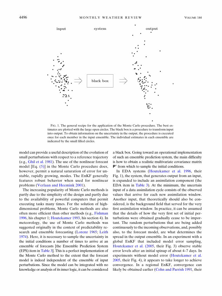
An example of a Monte Carlo application is shown in

Fig. 1. Here, we have a best estimate of the input and

output state and we want to know how the uncertainty in

the input state translates into uncertainty in an output

state. In NWP, we have a numerical tool, like a forecast

model, to generate an output from an input. By running

the tool once for each input, we can obtain an ensemble

of outputs. The only new utility required for running a

Monte Carlo experiment is the tool to generate an en-

semble of inputs. Note, in addition, that Monte Carlo

experiments can be performed in sequence, with the

output ensemble of one experiment serving as input en-

semble for the next experiment. In this case, instead of

specifically following a best estimate and its uncertainty,

one can decide to always estimate a required probability

distribution from the available ensemble of estimates.

When a best estimate is also required, the ensemblemean

can be used for this purpose and the ensemble spread

should provide a reliable estimate of the error in the

mean. The basic assumption justifying the use of the

Monte Carlo method is that the uncertainty with respect

to our best estimate evolves in almost the sameway as the

uncertainty with respect to the true state (Press et al.

1992, their section 15.6). This is similar to the assumption

underlying the extended Kalman filter that a linearized

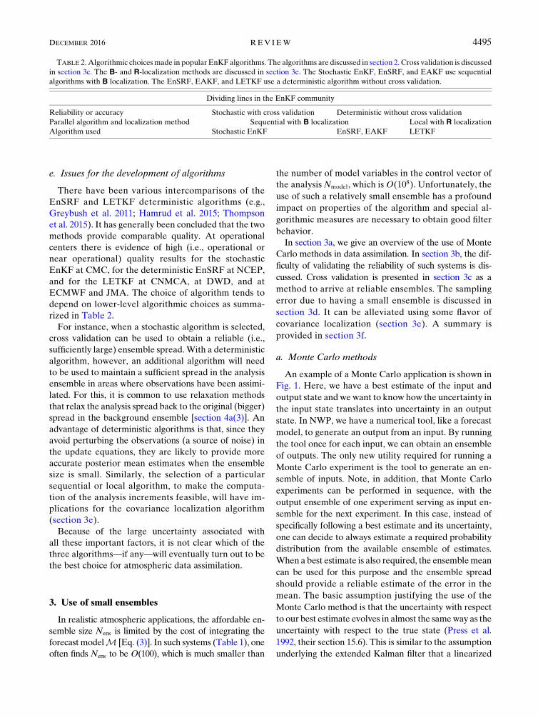
TABLE 2.Algorithmic choicesmade in popular EnKF algorithms. The algorithms are discussed in section 2. Cross validation is discussed

in section 3c. The B- and R-localization methods are discussed in section 3e. The Stochastic EnKF, EnSRF, and EAKF use sequential

algorithms with B localization. The EnSRF, EAKF, and LETKF use a deterministic algorithm without cross validation.

Dividing lines in the EnKF community

Reliability or accuracy Stochastic with cross validation Deterministic without cross validation

Parallel algorithm and localization method Sequential with B localization Local with R localization

Algorithm used Stochastic EnKF EnSRF, EAKF LETKF


model can provide a useful description of the evolution of

small perturbations with respect to a reference trajectory

(e.g., Ghil et al. 1981). The use of the nonlinear forecast

model [Eq. (5)] in the Monte Carlo procedure does,

however, permit a natural saturation of error for un-

stable, rapidly growing, modes. The EnKF generally

features robust behavior when used for nonlinear

problems (Verlaan and Heemink 2001).

The increasing popularity of Monte Carlo methods is

partly due to the simplicity of the design and partly due

to the availability of powerful computers that permit

executing tasks many times. For the solution of high-

dimensional problems, Monte Carlo methods are also

often more efficient than other methods (e.g., Fishman

1996, his chapter 1; Houtekamer 1993, his section 4). In

meteorology, the use of Monte Carlo methods was

suggested originally in the context of predictability re-

search and ensemble forecasting (Lorenz 1965; Leith

1974). Here, it is necessary to sample the uncertainty in

the initial conditions a number of times to arrive at an

ensemble of forecasts [the Ensemble Prediction System

(EPS) item in Table 3]. This is a perfect implementation of

the Monte Carlo method to the extent that the forecast

model is indeed independent of the ensemble of input

perturbations. Since the model can be integrated with no

knowledge or analysis of its inner logic, it can be considered

a black box. Going toward an operational implementation

of such an ensemble prediction system, the main difficulty

is how to obtain a realistic multivariate covariance matrix

Pa from which to sample the initial conditions.

In EDA systems (Houtekamer et al. 1996, their

Fig. 1), the system, that generates output from an input,

is expanded to include an assimilation component (the

EDA item in Table 3). At the minimum, the uncertain

input of a data assimilation cycle consists of the observed

values that arrive for each new assimilation window.

Another input, that theoretically should also be con-

sidered, is the background field that served for the very

first assimilation window. In practice, it can be assumed

that the details of how the very first set of initial per-

turbations were obtained gradually cease to be impor-

tant. The random perturbations that are being added

continuously to the incoming observations, and, possibly

also, to the forecast model, are what determines the

spread in the output ensemble. In an experiment with a

global EnKF that included model error sampling,

Houtekamer et al. (2005, their Fig. 3) observe stable

error levels after an initial spinup of about 4–7 days. In

experiments without model error (Houtekamer et al.

2005, their Fig. 4), it appears to take longer to achieve

convergence. In a regional EnKF, convergence can

likely be obtained earlier (Cohn and Parrish 1991, their

FIG. 1. The general recipe for the application of the Monte Carlo procedure. The best es-

timates are plotted with the large open circles. The black box is a procedure to transform input

into output. To obtain information on the uncertainty in the output, the procedure is executed

once for each member in the input ensemble. The individual estimates in each ensemble are

indicated by the small filled circles.


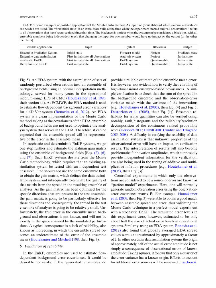
Fig. 5). An EDA system, with the assimilation of sets of

randomly perturbed observations into an ensemble of

background fields using an optimal interpolation meth-

odology, served for many years in the operational

medium-range EPS of CMC (Houtekamer et al. 1996,

their section 4a). At ECMWF, the EDAmethod is used

to estimate flow-dependent background error variances

for a 4D-Var system (Bonavita et al. 2012). An EDA

system is a clean implementation of the Monte Carlo

method as long as the covariances of the EDA ensemble

of background fields are not used to optimize the anal-

ysis system that serves in the EDA. Therefore, it can be

expected that the ensemble spread will be representa-

tive of the error in the ensemble mean.

In stochastic and deterministic EnKF systems, we go

one step further and estimate the Kalman gain matrix

using the ensemble of background fields [Eqs. (2), (6),

and (7)]. Such EnKF systems deviate from the Monte

Carlo methodology, which requires that an existing as-

similation system be tested with an independent test

ensemble. One should not use the same ensemble both

to obtain the gain matrix, which defines the data assimi-

lation system, and subsequently to estimate the quality of

that matrix from the spread in the resulting ensemble of

analyses. As the gain matrix has been optimized for the

specific directions that are present in the test ensemble,

the gain matrix is going to be particularly effective for

these directions and, consequently, the spread in the test

ensemble of analyses is going to be relatively small. Un-

fortunately, the true error in the ensemble mean back-

ground and observations is not known, and will not be

exactly in the space spanned by the simulated perturba-

tions. A typical consequence is a lack of reliability, also

known as inbreeding, in which the ensemble spread be-

comes an underestimate of the error of the ensemble

mean (Houtekamer and Mitchell 1998, their Fig. 3).

b. Validation of reliability

In the EnKF, ensembles are used to estimate flow-

dependent background error covariances. It would be

desirable to verify if the generated ensembles do

provide a reliable estimate of the ensemble mean error.

It is, however, not evident how to verify the reliability of

high-dimensional ensemble-based covariances. A sim-

ple verification is to check that the sum of the spread in

the background ensemble and the observation-error

variance match with the variance of the innovations

[e.g., Houtekamer et al. (2005), their Eq. (4) and Fig. 5;

Desroziers et al. (2005), their Eq. (1)]. Ensemble re-

liability for scalar quantities can also be verified using,

notably, rank histograms and the reliability/resolution

decomposition of the continuous ranked probability

score (Hersbach 2000;Hamill 2001; Candille andTalagrand

2005, 2008). A difficulty in verifying the reliability of data

assimilation systems is that unknown properties of the

observational error will have an impact on verification

results. The interpretation of results will also become

problematic if innovation amplitudes, which supposedly

provide independent information for the verification,

are also being used in the tuning of additive and multi-

plicative inflation procedures [e.g., Houtekamer et al.

(2005), their Eq. (3)].

Controlled experiments in which only the observa-

tions are considered to be a source of error are known as

‘‘perfect-model’’ experiments. Here, one will normally

generate random observation error using the observation-

error covariance matrix R. For example, Houtekamer

et al. (2009, their Fig. 3) were able to obtain a good match

between ensemble spread and error, thus validating the

Monte Carlo technique in a perfect-model experiment

with a stochastic EnKF. The simulated error levels in

this experiment were, however, estimated to be only

about half the size of actual error levels in operational

systems. Similarly, using an EDA system, Bonavita et al.

(2012) also found that globally averaged EDA spread

values were underestimated by approximately a factor

of 2. In other words, in data assimilation systems the origin

of approximately half of the actual error amplitude is not

simply a consequence of observational errors of known

amplitude. Taking squares, it follows that only a quarter of

the error variance has a known origin. Efforts to account

for additional error sources will be reviewed in section 4.

TABLE 3. Some examples of possible applications of the Monte Carlo method. As input, only quantities of which random realizations

are needed are listed. The ‘‘first initial state’’ is an initial state valid at the time when the experiment started and ‘‘all observations’’ refers

to all observations that have been received since that time. The blackness is perfect when the system can be considered a black box, with all

ensemble members being independent (such that changing the input for one member would have no impact on the output for the other

members).

Possible application Input System Blackness Output

Ensemble Prediction System Initial state Forecast model Perfect Predicted state

Ensemble data assimilation First initial state all observations Analysis system Perfect Initial state

Stochastic EnKF First initial state all observations EnKF system Questionable Initial state

Deterministic EnKF First initial state EnKF system Questionable Initial state


A fairly high natural error level in perfect-model ex-

periments would suggest that Eqs. (1) and (3) provide a

fairly reasonable set of equations for the evolution of

errors in the system, and could thus be seen as a justifi-

cation for the use of a costly 4D assimilation system,

such as 4D-Var and the EnKF. Given the modest frac-

tion of error sources of known and quantifiable origin, it

is perhaps surprising that operationally interesting re-

sults can already be obtained with the current genera-

tion of 4D assimilation systems.

c. Use of group filters with no inbreeding

As mentioned in section 3a, the use of a Monte Carlo

ensemble to estimate the Kalman gain can lead to in-

breeding in which the ensemble spread becomes a sys-

tematic underestimate of the error of the ensemble

mean. In the context of a stochastic EnKF, it is possible

to counter this problem using k-fold cross validation

(Houtekamer andMitchell 1998;Mitchell andHoutekamer

2009). Here, the original ensemble is divided into k sub-

ensembles of equal size. To assimilate observations into

one subensemble of background fields one uses a gain

matrix computed from other, independent, members. In

the limiting case of leave-one-out cross validation, the

subensembles consist of only one member (Hamill and

Snyder 2000). As a result of cross validation, it is possible,

at least in perfect-model environments, to maintain a

representative ensemble in which the ensemble spread is

an unbiased estimate of the ensemble mean error (e.g.,

Houtekamer et al. 2009, their Fig. 3). Whitaker and

Hamill (2002, their appendix) give an example of twofold

cross validation for a deterministic filter. Although com-

paratively good results were obtained, the algorithm had a

very substantial computational cost and has not been

pursued further.

When cross validation is used to obtain a reliable

ensemble, not all members are used in the computation

of the gain for a subensemble. Alternatively, one can

use a single ensemble configuration in which all avail-

able members are used to compute a single gain matrix.

This matrix will likely be more accurate, since the use of

more members leads to less sampling error. Comparing

the single ensemble and cross-validation approaches, it

has been found that the single ensemble, while being less

reliable, may well have an ensemble mean of similar or

better quality, when the number k of subensembles that

is used in the cross validation is small, but tends to have

an ensemble mean of poorer quality when the number k

of subensembles is large (Mitchell and Houtekamer

2009, their Figs. 2 and 3). In the case of dense observa-

tions that are only weakly correlated with the model

state, cross validation can signal degraded quality via an

increase of the ensemble spread. This can even lead to

catastrophic filter divergence in which the ensemble spread

becomes excessively large (Houtekamer andMitchell 2005,

their section 3b). See appendix A for a more comprehen-

sive discussion of filter divergence in EnKF systems.

Related to cross validation is the hierarchical filter

(Anderson 2007). Here the observations are assimilated

sequentially, one at a time. At each step of the sequen-

tial algorithm, an ensemble of EnKFs is run to obtain a

confidence factor for the regression coefficient in the

scalar Kalman gain K. These factors can subsequently

serve toward the generation of more optimal localiza-

tion functions.

d. Sampling error due to limited ensemble size: Therank problem

In the original Kalman filter equations, the matrix P f

is full rank. To obtain this matrix, one would need to

integrate the tangent linear model once for each of the

Nmodel ’ O(100 000 000) coordinates of the numerical

model M. While this would be an expensive proposi-

tion, it would provide us with Nmodel different directions

in phase space (i.e., the Nmodel eigenvectors of Pf ), for

which observations could be used toward a reduction of

the uncertainty. In addition, the eigenvectors with sig-

nificant eigenvalues can be expected to locally follow the

attractor of the model, since they have been obtained

using model integrations.

An EnKF system with Nens ’O(100) members only

provides Nens 2 1 directions in phase space. Thus, the

information in the Nobs observations, with Nobs typically

O(1 000 000), must be projected onto a small number of

directions (Lorenc 2003, his section 3b). The fact that

Nens � Nmodel and Nens � Nobs is commonly known as

the rank problem; it is themost important approximation/

difference with respect to the Kalman filter. How exactly

this issue is dealt with has a major impact on the char-

acteristics of an EnKF implementation.

It may be noted that the rank problem is not unique to

EnKF systems. For variational data assimilation sys-

tems, the NMC method (Parrish and Derber 1992) or

the EDA method (Bonavita et al. 2012) typically pro-

vides an ensemble ofO(100) error directions that can be

used in the estimate of a matrix P f . In this case, co-

variance modeling is used to make P f full rank. Such

modeling is obtained by means of a sequence of well-

designed coordinate transformations. Fisher (2004)

showed how a wavelet-based covariance model can be

used to obtain spatially varying vertical and horizontal

correlations. Flow-dependent dynamical balances could

also be included. The authors are not aware of reports

on rank issues encountered in the subsequent assimila-

tion of O(10 000 000) observations. How to similarly

extend the low-rank background ensemble of an EnKF


into a flow-dependent high-rank matrix for subsequent

use in an EnKF data assimilation system is a major

problem that, as we will see, is still not well resolved.

e. Covariance localization

To address the rank problem (section 3d), an intuitive

solution is to split the global data assimilation problem

into a number of quasi-independent local problems. For

each of the local problems, the Nens 2 1 local directions

of the ensemble may permit a fairly relevant approxi-

mation of the true uncertainty (Oczkowski et al. 2005).

Houtekamer and Mitchell (2005, their section 5b) esti-

mated that, with localization, a 96-member ensemble of

global fields can provide an effective dimensionality of

over 10 000. In fact, localization is the critical approxi-

mation that makes Monte Carlo methods a feasible

proposition for the solution of the Kalman filter equa-

tions in large problems. There is a consensus in the at-

mospheric data assimilation community that localization

is an essential component of an EnKF algorithm (Hamill

et al. 2001; Anderson 2012). As larger ensembles become

available, it will likely be optimal to use a less severe

covariance localization (Houtekamer and Mitchell 1998,

their Fig. 5; Miyoshi et al. 2014).

How localization is implemented exactly is often fairly

ad hoc and depends on the particular EnKF algorithm that

is used. In the implementation byHoutekamer andMitchell

(1998), observations are not used if their distance from

an analysis grid point exceeds some critical value.

Similarly, in an LETKF, it is natural to exclude ob-

servations beyond a certain distance from the local

analysis domain.

1) LOCALIZATION IN THE SEQUENTIAL FILTER

In a sequential filter, localization can be implemented

using the product of the ensemble-based covariances

with a smooth correlation function r [Houtekamer and

Mitchell (2001), their Eq. (6)]:

K5 [r+(P fHT)][r+(HP fHT)1R]21 , (19)

where the symbol + denotes the Schur (element-wise)

product of two matrices and r is a function of the dis-

tance d between two items. For the localizing term in the

numerator of Eq. (19), which multiplies P fHT, it is thus

necessary to define the distance between observations

and model coordinates. For the term in the de-

nominator, which multiplies HP fHT, only the distance

between different observations is needed. Note that

there can be both integral model variables, such as sur-

face pressure, and integral observation variables, such as

satellite radiances, for which it is not clear how to

define a location in space.

For the localizing correlation function r, it is common

to use the compactly supported fifth-order piecewise

rational function proposed by Gaspari and Cohn

[(1999), their Eq. (4.10)]. This function looks like a

Gaussian and depends on a single length scale parame-

ter. The compact support leads to zero impact of an

observation beyond a certain distance. This property can

be exploited to reduce computational cost. Note, how-

ever, that without a localization step, it would be possible

to perform matrix operations in a different order for a

more efficient algorithm [Mandel (2006), his Eq. (4.1);

Houtekamer et al. (2014b), their section 4b(6)]. With the

significant vertical extent of the model domain, it is ad-

vantageous to use localization in both horizontal and ver-

tical directions [Houtekamer et al. (2005), their Eq. (2)]:

K5 [rV+r

H+(P fHT)][r

V+r

H+(HP fHT)1R]21 ,(20)

where rV and rH are the correlation functions for the

vertical and horizontal localizations, respectively.

Multiplication with a localizing function is not part of

Kalman filter theory; therefore, some of the properties

of the Kalman filter do not carry over to an EnKF with

localization. One of these properties is the equivalence

between processing observations either serially or all at

once [section 2c(1)]. The analysis increments will also

not be exactly in the space spanned by the background

ensemble. The associated imbalance, and return to the

model attractor, may lead to rapid adjustment in the

forecasts initiated from the analyses.

2) LOCALIZATION IN THE LETKF

In an LETKF, calculations are done in ensemble

space and consequently the matrix P f is not represented

in physical space. Thus, it is not possible to use Eq. (19)

to obtain localized analysis increments. Hunt et al.

(2007) proposed to localize instead by gradually in-

creasing observation-error variances for remote obser-

vations using the positive exponential function:

fRloc

5 exp

"1d(i, j)2

2L2

#, (21)

where d(i, j) is the distance between observation i and

model grid point j, and L is the length scale parameter

for the localization.

Greybush et al. (2011) compared the R localization of

Eq. (21) with the B localization of Eq. (19). They found

the B localization to be more severe than the R locali-

zation when the same length scales are used in the lo-

calizing functions, and consequently, the optimal

localization length was found to be longer for the B lo-

calization. When each scheme was used with its optimal


localization length, they found the two techniques to be

comparable in performance with respect to both rms

analysis error and balance. Sakov and Bertino (2011)

also find that the two localization methods should pro-

vide very similar results in practice. They note, however,

more robust behavior for the B localization in the spe-

cial case of ‘‘strong’’ data assimilation (i.e., when the

analysis causes a big reduction in the uncertainty).

3) ISSUES WITH LOCALIZATION

Localization has been presented as a way to imple-

ment an approximation to the optimal Kalman filter

with a small [Nens 5O(100)] number of ensemble

members. It would appear that the severity of the lo-

calization is also determined by the desire to maintain

physical balances, such as geostrophy or hydrostatic

balance, in the analyses (Cohn et al. 1998; Lorenc 2003).

To maintain geostrophic balance in a global data as-

similation system, Mitchell et al. (2002) suggested lim-

iting the impact of observations to a distance not smaller

than about 3000km. Within a region of this size, the

ensemble can only provide Nens 2 1 directions in phase

space. The a priori expectation is that with higher-

resolution models and with increasing numbers of ob-

servations, it will be necessary to increaseNens to permit

balanced analysis increments that cover both large and

small scales. This trend is illustrated by the evolution of

the operational EnKF at CMC which, as of November

2014, has a horizontal resolution of 50 km as well as a

fairly sizable ensemble with Nens 5 256 members. In

scaling experiments for hypothetical future EnKF con-

figurations (Houtekamer et al. 2014b), the maximum

ensemble size was Nens 5 768. Ensemble sizes of

O(1000) have not historically been considered to be

reasonable and may indicate a need for major algorith-

mic changes. In the currently operational CMC EnKF,

the cutoff distance for observations is, depending on the

height in the atmosphere, between 2100 and 3000km

(Houtekamer et al. 2014a, their Table 3). For the NCEP

EnKF, with 80members, a shorter distance of 1600 km is

used (X. Wang et al. 2013, their section 2). This reflects

that optimal localizaton distances are found after ex-

perimentation considering a number of factors, of which

balance is only one.

In the successive covariance localization (SCL; Zhang

et al. 2009a) algorithm, a sequential EnKF is used to first

assimilate large-scale information from a small subset of

observations using broad localization functions and

subsequently smaller-scale features are obtained from

larger sets of observations using tighter correlation

functions. Proceeding in three steps, the procedure

permits obtaining a detailed hurricane analysis including

mesoscale vortices in a reasonably balanced large-scale

environment. The SCL technique requires some prior

knowledge of the characteristic and dynamic scales of

the phenomena of interest. It remains a challenge, for

example, how to use convective area observations to

update environmental (cloud free) state variables for

convective storm analysis and prediction.

A similar pragmatic procedure can be applied in the

vertical, using severe localization for conventional ob-

servations, moderate localization for surface pressure

observations, and broad localization for satellite obser-

vations reflecting the nonlocal nature of the latter

(X. Wang et al. 2013). Also, because horizontal length

scales generally increase with height in the atmosphere,

horizontal localization lengths can be made to increase

with height as in Houtekamer et al. (2014a, their Table 3)

and Kleist and Ide (2015a, their Fig. 3).

A more dramatic algorithmic change is provided by

the ensemble multiscale filter of Zhou et al. (2008),

which effectively replaces, at each analysis time, the

prior sample covariance with a multiscale tree. This

permits tracking changing features over long distances

without spatial localization. For large problems, this

method provides a hybrid localization in both space and

scale. With a variational solver, Buehner (2012) com-

pared spatial localization, spatial/spectral localization,

and wavelet-diagonal approaches. The comparative

performance was found to depend on ensemble size.

With a 48-member ensemble, spatial/spectral localiza-

tion gave the best results. With a 12-member ensemble,

the wavelet-diagonal approach performed best.

It would of course be desirable (if possible) to have

some guiding principle in the choice of a localization

method. It could, for instance, be defined as the opera-

tion that minimizes the analysis error given a certain

limited ensemble size (Zhen and Zhang 2014; Flowerdew

2015). There are, for now, no known analytical methods

to derive such an operation for complex situations with

multiple observations. Anderson (2007) shows, with his

hierarchical filter, that the optimal localization for spa-

tially averaged observations can be quite different from a

smooth Gaspari–Cohn function. The method could also

be used to determine the significance of correlations be-

tween variables of different type. Note that, in variational

methods, it is common to specify a zero covariance be-

tween background errors of temperature and specific

humidity. Localization between different variables was

first applied in an EnKF in the context of a carbon cycle

assimilation system (Kang et al. 2011). Here, nonzero

error covariances were allowed between CO2 and the

wind field, which affects transport of CO2, but not be-

tween CO2 and other meteorological variables. This

procedure effectively filters the noisy ensemble-based

correlations between physically unrelated variables. Lei


and Anderson (2014) propose using empirical localiza-

tion functions (ELFs) determined from OSSEs to give

appropriate localization for any potential observation

type and kind of state variable. A perhaps more practical

approach is to use, as an assimilation cycle proceeds,

improving prior estimates of the correlation between

classes of variables (Anderson 2016). These prior esti-

mates and the estimated flow-dependent correlations are

subsequently combined to obtain a posterior estimate

that is to be used to compute analysis increments.

Lange and Craig (2014) present high-resolution data

assimilation experiments for convective storms. Here,

with a 5-min assimilation window and a localization

cutoff length of 8 km, the scales are more than an order

of magnitude different from global data assimilation

scales and geostrophic balance is perhaps no longer a

relevant concept. Nevertheless, similar problems are

noted in that severe localization causes imbalance and

some sort of adjustment that may degrade subsequent

forecasts.

f. Summary

In perfect-model environments, using a stochastic al-

gorithm and cross validation, it is possible to reliably

simulate error evolution. In deterministic filters, reliable

ensembles can also be obtained, but it is necessary to

add an algorithm to relax the underdispersive analysis

spread back to the prior spread [section 4a(3)]. How to

best verify reliability of realistic EnKF systems in a di-

rect and informative manner is still an open issue.

Nevertheless, reliability is a highly desirable feature of

ensemble systems. Using a small ensemble, the large

spread in a reliable EnKF would reliably show that the

analysis quality is low. With increased ensemble size,

the reduced spread would reflect the reduced error in the

ensemble mean. It does greatly facilitate development

work if such changes to the EnKF are reliably reflected in

changed ensemble spread (Houtekamer et al. 2014a, their

section 6). Whereas such reliability of an EnKF is desir-

able, it does not in itself guarantee high analysis quality. It

is, in principle, possible to have an unreliable EnKF al-

gorithm that, for a given ensemble size, provides smaller

ensemble mean errors than a corresponding reliable al-

gorithm (Houtekamer and Mitchell 1998, the middle

panels of their Fig. 3).

To obtain high-quality analyses with a small ensem-

ble, it is necessary to localize the analysis increments.

We have seen various ways to localize the ensemble

covariances using tapering functions that reduce analy-

sis increments associated with distant observations to

zero. Unfortunately, a certain amount of experimenta-

tion will often be necessary to arrive at an optimal length

scale for the tapering function. With grids covering a

range of scales that are being observed with a hetero-

geneous observational network, one would like to have a

more flexible and general algorithm for covariance lo-

calization. How to best proceed is still an unresolved is-

sue. Ideally, of course, onewould be able use an ensemble

that is so large that details of the localization method (if

any) do not matter (Miyoshi et al. 2014).

4. Methods to increase ensemble spread

As discussed in section 3b, assuming that the forecast

model is perfect, and that errors are solely due to

propagation of observational error in the assimilation

cycle, both EnKF and EDA studies show that the re-

sulting ensembles explain only about a quarter of the

error variance of the ensemble mean. In this section, we

will describe methods that can be used to arrive at more

realistic levels of spread.

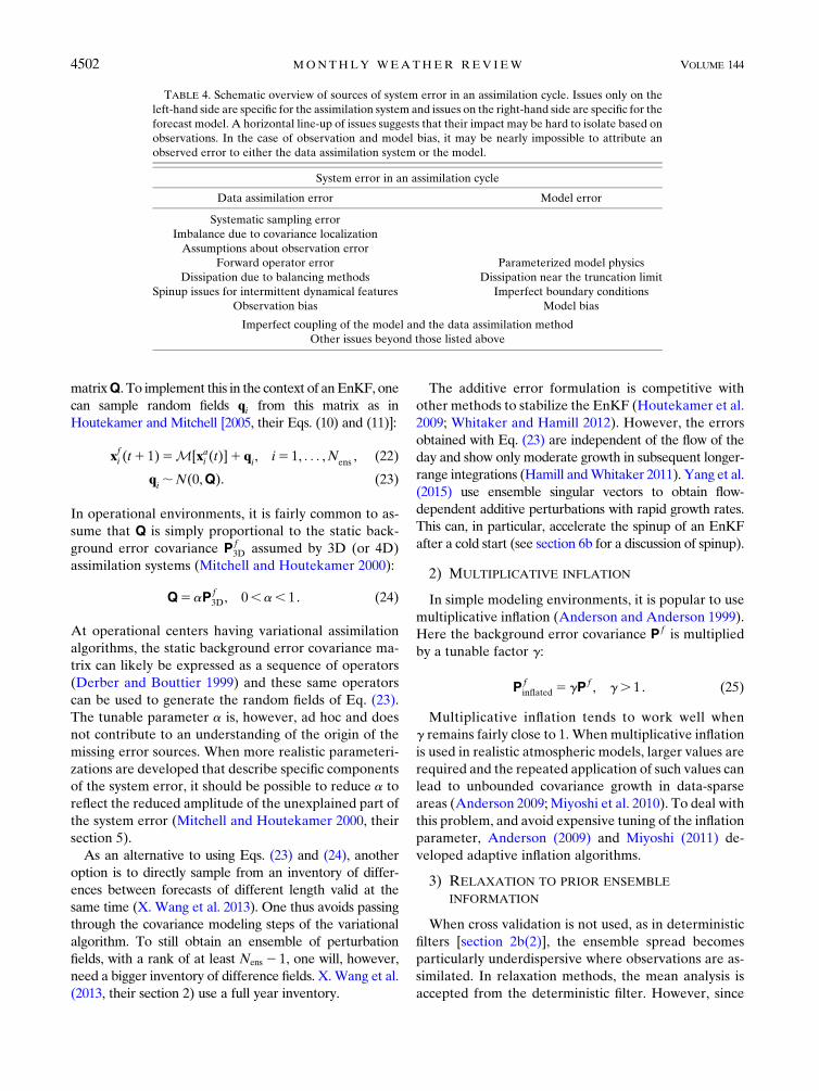
We refer (see Table 4) to error sources associated with

the forecast model [i.e., Eq. (3)] as ‘‘model error’’ and to

error sources associated with the computation of the

analysis increment [Eq. (1)] as ‘‘data assimilation error.’’

Errors whose origin is unknown, but that could originate

either in the forecast model or the data assimilation step

will be referred to as ‘‘system error’’ (Houtekamer and

Mitchell 2005).

Various flavors of covariance inflation, discussed in

section 4a, provide bulk methods of changing the en-

semble spread to a desired level with no knowledge of

the corresponding specific error sources. Other methods

aim at specifically increasing spread where a problem is

known to exist. For example, stochastic kinetic energy

backscatter (section 4b) reintroduces error variance that

had been lost due to diffusive processes. Errors associated

with model physical parameterizations are discussed in

section 4c. We end (section 4d) with a discussion of the

realism of current methods to arrive at realistic error levels.

a. Covariance inflation

The oldest method to increase ensemble spread, dis-

cussed in section 4a(1), is inspired by Kalman filter

theory and consists of adding perturbation fields ob-

tained using prescribed model error covariances. An

alternative method, that is convenient in simple mod-

eling environments, is to multiply perturbations with a

constant inflation factor [section 4a(2)]. Finally, relaxation

methods have been developed to address underdispersion

in deterministic filter systems [section 4a(3)].

1) ADDITIVE INFLATION

In Kalman filter theory, it is standard (e.g., Cohn and

Parrish 1991; Dee 1995) to assume that the forecast-

model error is white in time, withmean zero and covariance


matrixQ. To implement this in the context of anEnKF, one

can sample random fields qi from this matrix as in

Houtekamer and Mitchell [2005, their Eqs. (10) and (11)]:

xfi (t1 1)5M[xai (t)]1 qi, i5 1, . . . ,N

ens, (22)

qi;N(0,Q). (23)

In operational environments, it is fairly common to as-

sume that Q is simply proportional to the static back-

ground error covariance P f3D assumed by 3D (or 4D)

assimilation systems (Mitchell and Houtekamer 2000):

Q5aP f3D, 0,a, 1. (24)

At operational centers having variational assimilation

algorithms, the static background error covariance ma-

trix can likely be expressed as a sequence of operators

(Derber and Bouttier 1999) and these same operators

can be used to generate the random fields of Eq. (23).

The tunable parameter a is, however, ad hoc and does

not contribute to an understanding of the origin of the

missing error sources. When more realistic parameteri-

zations are developed that describe specific components

of the system error, it should be possible to reduce a to

reflect the reduced amplitude of the unexplained part of

the system error (Mitchell and Houtekamer 2000, their

section 5).

As an alternative to using Eqs. (23) and (24), another

option is to directly sample from an inventory of differ-

ences between forecasts of different length valid at the

same time (X. Wang et al. 2013). One thus avoids passing

through the covariance modeling steps of the variational

algorithm. To still obtain an ensemble of perturbation

fields, with a rank of at least Nens 2 1, one will, however,

need a bigger inventory of difference fields. X.Wang et al.

(2013, their section 2) use a full year inventory.

The additive error formulation is competitive with

other methods to stabilize the EnKF (Houtekamer et al.

2009; Whitaker and Hamill 2012). However, the errors

obtained with Eq. (23) are independent of the flow of the

day and show only moderate growth in subsequent longer-

range integrations (Hamill andWhitaker 2011). Yang et al.

(2015) use ensemble singular vectors to obtain flow-

dependent additive perturbations with rapid growth rates.

This can, in particular, accelerate the spinup of an EnKF

after a cold start (see section 6b for a discussion of spinup).

2) MULTIPLICATIVE INFLATION

In simple modeling environments, it is popular to use

multiplicative inflation (Anderson and Anderson 1999).

Here the background error covariance P f is multiplied

by a tunable factor g:

P finflated 5 gP f , g. 1. (25)

Multiplicative inflation tends to work well when

g remains fairly close to 1. When multiplicative inflation

is used in realistic atmospheric models, larger values are

required and the repeated application of such values can

lead to unbounded covariance growth in data-sparse

areas (Anderson 2009; Miyoshi et al. 2010). To deal with

this problem, and avoid expensive tuning of the inflation

parameter, Anderson (2009) and Miyoshi (2011) de-

veloped adaptive inflation algorithms.

3) RELAXATION TO PRIOR ENSEMBLE

INFORMATION

When cross validation is not used, as in deterministic

filters [section 2b(2)], the ensemble spread becomes

particularly underdispersive where observations are as-

similated. In relaxation methods, the mean analysis is

accepted from the deterministic filter. However, since

TABLE 4. Schematic overview of sources of system error in an assimilation cycle. Issues only on the

left-hand side are specific for the assimilation system and issues on the right-hand side are specific for the

forecast model. A horizontal line-up of issues suggests that their impact may be hard to isolate based on

observations. In the case of observation and model bias, it may be nearly impossible to attribute an

observed error to either the data assimilation system or the model.

System error in an assimilation cycle

Data assimilation error Model error

Systematic sampling error

Imbalance due to covariance localization

Assumptions about observation error

Forward operator error Parameterized model physics

Dissipation due to balancing methods Dissipation near the truncation limit

Spinup issues for intermittent dynamical features Imperfect boundary conditions

Observation bias Model bias

Imperfect coupling of the model and the data assimilation method

Other issues beyond those listed above


the ensemble spread obtained using Eq. (10) is known to

be too small, only part of the proposed spread reduction

is accepted for the ensemble of perturbations.

A formulation that only changes the analysis where

data have been assimilated is the relaxation to prior

perturbation (RTPP)method of Zhang et al. [2004, their

Eq. (5)]. Here the computed analysis perturbations

xai 2 xa are relaxed back to the prior perturbations

x fi 2 xf using the following:

xai,new 2 xa 5 (12a)(xai 2 xa)1a(x fi 2 xf ), 0#a# 1.

(26)

In the limit a5 1, the analysis perturbations are identi-

cal to the background perturbations and, after a number

of assimilation cycles, the perturbations will gradually

converge to the leading Lyapunov (i.e., bred) vectors

(Toth and Kalnay 1997; Annan 2004; Whitaker and

Hamill 2012). Such an ensemble can be expected to

have a relatively low effective dimension. This would

not seem desirable because, in data assimilation, a

higher dimension would permit a more effective use of a

high volume of observations. The resulting ensemble

can, however, also be expected to have fairly good bal-

ance properties and high growth rates, which are both

desirable.

In the relaxation to prior spread (RTPS) algorithm

[Whitaker and Hamill (2012), their Eq. (2)], the en-

semble spread sa—as opposed to the ensemble of

perturbations—is relaxed back to the prior value sb

using the following:

sanew 5 (12a)sa 1asb, 0#a# 1. (27)

Ying and Zhang (2015) propose an adaptive algorithm

to determine the a parameter of the RTPS method, and

tested it in the context of the Lorenz 40-variable model.

Tuning a real data assimilation system for optimal

performance, one may find best results with values of

a5 0:9, or even higher, in Eqs. (26) or (27). Such severe

relaxation or inflation indicates that the pure analysis

ensemble is not representative of the ensemble mean

analysis error and warrants further investigation. Notably,

convergence experiments with larger ensemble sizes can

be used to determine if the severe underdispersion is due

to the absence of cross validation or due to some

other cause.

Whitaker and Hamill (2012) recommend using re-

laxation methods [Eqs. (26) or (27)] to correct for data

assimilation errors, which will be more severe when

dense observations are available, and additive inflation

[Eq. (22)] to account for model error.

4) ISSUES WITH INFLATION

In operational environments, simple inflation methods

as discussed above are critical for maintaining sufficient

ensemble spread and having good overall performance

(Houtekamer et al. 2009; X. Wang et al. 2013). Unfortu-

nately, they will dilute the impact of the flow-dependent

statistics developed in the EnKF. It is important to de-

vote more effort to the identification of error sources in

the assimilation cycle; this should permit a more ap-

propriate error sampling and a reduced role of inflation

methods.

b. Diffusion and truncation

It has been found that models become more active

(i.e., start having faster intrinsic growth rates), when the

model resolution is increased and smaller scales can be

included. This has, for instance, been observed at

ECMWF with the so-called ‘‘Lorenz diagrams’’ [Fig. 1

in Lorenz (1982); Fig. 16 in Simmons (1996)]. These

show a more and more rapid growth of differences with

the model dynamics in medium-range forecasts as, in a

sequence of operational implementations over a num-

ber of years, the spatial resolution of the system is im-

proved. At the same time, the quality of the forecasts has

been consistently improved. In an ensemble context,

higher instrinsic growth rates of the model and reduced

error permit the simulation of a larger fraction of the

error with the internal dynamics of the forecast model.

Recent EnKF (Bonavita et al. 2015, their section 2) and

EDA (Bonavita et al. 2016, their section 4) experiments

at ECMWF show a desirable increase in ensemble

spread as resolution is increased. These various results

reflect that diffusion in the forecast model suppresses

activity in the smallest scales. As a result of this diffu-

sion, it can be difficult to maintain a suitable level of

spread in an EnKF system and subsequent EPS forecasts

(Mitchell et al. 2002, their section 5).

A similar diffusive effect can be the result of balancing

methods (see section 5 below and Table 4), which, while

necessary to obtain good performance, can filter the

signal associated with atmospheric tides as well as with

rapidly evolving weather systems.

To be realistic, it would be desirable to have an upscale

propagation of uncertainty from beyond the truncation

limit to the resolved scales. The stochastic kinetic energy

backscatter algorithm (SKEB; Shutts 2005) aims to ran-

domly reinsert kinetic energy that has been overdissipated

near the model truncation limit. The overdissipation can

be a consequence of explicit and implicit diffusion in the

model or of insufficient energy upscaling by parameteri-

zations for gravity wave breaking and deep convection

(Charron et al. 2010). The use of the SKEB algorithm has


generally been seen to have a positive impact in medium-

range ensemble prediction systems (Berner et al. 2009;

Charron et al. 2010).

In data assimilation systems, however, it has been

difficult to obtain a positive impact from the SKEB al-

gorithm (Houtekamer et al. 2009; Bonavita 2011). Even

when model truncation is known to be an important

source of error, it is hard to obtain better results with

SKEB than with simple additive inflation (Whitaker and

Hamill 2012).

In practice, when implementing the SKEB algorithm,

many choices need to be made. These include the choice

and quantification of processes responsible for the drag,

the fraction of dissipated energy that needs to be rein-

troduced, the spectrum in space and time for the back-

scatter, and the modes (rotational or gravity) on which

the perturbations are to be added. In amesoscale EnKF,

Ha et al. (2015) did obtain good results by perturbing the

largest scales, going down to an estimated effective

resolution of 6Dx, with a spatially and temporally con-

stant formulation. Since it is neither flow dependent nor

scale selective, this SKEB implementation is in fact

similar to the additive formulation of Eq. (22), with the

noise being added at every model time step (Ha et al.

2015, their section 3a). Recently, Shutts and Callado

Pallares (2011) suggested using the related vorticity

confinement algorithm (Steinhoff and Underhill 1994)

as an alternative to SKEB.

c. Error in physical parameterizations

In this subsection, we will review error that can be

associated with the physical parameterizations of the

forecast model. This subject has been extensively in-

vestigated in the context of medium-range ensemble

prediction systems.Many operational centers contribute

with their medium-range ensemble forecasts to the

TIGGE project (Swinbank et al. 2015, their Table 1). As

shown by online verifications of TIGGE data on the

‘‘TIGGEMuseum’’ (e.g., http://gpvjma.ccs.hpcc.jp/TIGGE/

tigge_scatter_diagram.html), state-of-the-art systems now

maintain a reasonable agreement between spread and

error. Many popular methods have been discussed in the

proceedings of the 2011 ECMWF workshop on repre-

sentingmodel uncertainty and error in numerical weather

and climate prediction models (ECMWF 2011). It would

be a priori preferable—if only for considerations of

consistency, model spinup, and balance—to use the same

treatment of model error in both data assimilation and

subsequent medium-range forecast applications. How-

ever, as noted by Bonavita (2011), the data assimilation

environment is more challenging than the medium-range

ensemble prediction environment. This is in part because

background errors, which have not yet converged to the

dominant modes of instability of the system (Wei and

Toth 2003), span a higher dimensional space than longer-

lead forecast errors. Another reason is that data assimi-

lation applications require multivariate covariances,

whereas the users of EPS forecasts are mostly interested

in the mean and standard deviation of scalar forecast

variables. It is thus not a priori clear that algorithms,

which have been developed and proven successful in

medium-range applications, will also be beneficial in

data assimilation applications.

1) PHYSICAL TENDENCY PERTURBATIONS

To reflect the uncertainty in parameterized physical

processes, Buizza et al. (1999) developed a stochastic

algorithm for the perturbation of tendencies of the

model physics (SPTP). Here, the output Pj of the model

physics for member j is multiplied by a random num-

ber rj to provide a perturbed output P0j of the model

physics:

P0j(t)[ r

j(f, l, t)P

j(t) . (28)

In the original paper, the random number rj was drawn

from a uniform distribution between 0.5 and 1.5, with

different values being used every 108 latitude–longitudein space and every 6h in time. The algorithm was shown

to increase spread and improve probabilistic scores. It

has since been refined using a number of different time

scales and a spectral pattern generator of the type de-

scribed by Li et al. (2008), and is also in use at CMC

(Charron et al. 2010).

Experiments with SPTP in an EnKF context

(Houtekamer et al. 2009) were not conclusive. Similarly,

Bonavita (2011) concluded that ‘‘it may be the case that

the spatially correlated error structures introduced by

the model error schemes do not represent background

error covariances well. Further investigations are re-

quired on this issue.’’

One issue with Eq. (28) is that for rj 6¼ 1 it forces an

inconsistency between the deterministic model physics

Pj(t) and the applied tendencies P0j(t). In extreme cases,

this can lead to unstable behavior of the model physics

(e.g., Working Group 1, p. viii, ECMWF 2011) and, for

instance, motivate a reduction of the amplitude of the

random perturbations near the surface. There is also

little theoretical support for the simple proportionality

between the amplitude of tendency and of the error

simulated by Eq. (28) (Shutts and Callado Pallares 2011,

their Fig. 1). More refined formulations of SPTP, which

could use information about the uncertainty in specific

physical processes, would also need to consider corre-

lations between errors in these processes and be con-

siderably more complex.


http://gpvjma.ccs.hpcc.jp/TIGGE/tigge_scatter_diagram.html

http://gpvjma.ccs.hpcc.jp/TIGGE/tigge_scatter_diagram.html

2) MULTIMODEL, MULTIPHYSICS, AND

MULTIPARAMETER APPROACHES

A pragmatic approach to model error sampling is to

use multiple models, multiple physical parameteriza-

tions, or multiple parameter values (Krishnamurti et al.

1999). In the EPS context, a substantial gain has been

seen from combining medium-range ensemble forecasts

from different NWP centers (Mylne et al. 2002; Candille

2009). In an operational data assimilation context, such

an approach would require a rapid exchange between

centers of a large number of analysis and trial fields. In

addition, one would have to resolve potentially complex

issues associated with using different definitions for

grids and variables. Of course, to obtain a high-rank

sampling of model error, it could be necessary to use

more than two different models. The approach has, to

the knowledge of the authors, not been tried in an

ensemble-based assimilation context.

The use ofmultiphysics approaches, which are simpler

to implement, generally has a positive impact also in

ensemble-based data assimilation approaches (Fujita

et al. 2007; Meng and Zhang 2007, 2008a,b; Houtekamer

et al. 2009). The use of multiple physical parameteriza-

tions does, in particular, permit the sampling of different

possible closure assumptions in deep convection and in

boundary layer processes. At operational centers, the

multiphysics approach is used in a fairly ad hoc manner

to sample uncertainty (Houtekamer 2011) as opposed to

being an integral component of the development of

state-of-the-art physical parameterizations (Houtekamer

and Lefaivre 1997). As part of a multiphysics ensemble, it

is possible to also perturb various parameters that play a

role in the model physical parameterizations. In the Met

Office Global and Regional Ensemble Prediction System

(MOGREPS) short-range EPS, for example, eight

parameters are perturbed using a stochastic first-order

autoregressive process (Bowler et al. 2008, their section

4.1). The multiparameter approach has been pursued

systematically in the context of climate projections

(Murphy et al. 2011).

Using an extended-state-vector approach, model pa-

rameters can be estimated simultaneously with the state

variables (e.g., Annan et al. 2005; Aksoy et al. 2006; Ruiz

and Pulido 2015). One difficulty is that model parame-

ters usually have a global impact whereas an EnKF will

use localization to obtain local estimates for the pa-

rameters. A unique parameter value will then usually be

obtained using a global averaging procedure. Note that

we will see the same issue in the context of bias cor-

rection for radiance observations (section 7c). Since

there is no natural unstable model to make the estimated

parameter uncertainty grow in time along dynamical

modes, as in Eq. (3), the estimated parameter values can

quickly converge to values that are no longer affected

much by new data. To prevent this classical type of filter

divergence (see appendix A for more discussion), a con-

ditional covariance inflation can be used to maintain the

estimated uncertainty at a desired level (Aksoy et al. 2006).

When estimatingmultiple parameters, another challenge is

that errors associated with individual parameters tend to

counterbalance each other in many complicated ways

(Aksoy et al. 2006). In fact, model failuremay occur due to

numerically unstable combinations of parameters. De-

spite the relative power of the estimation procedure, to

ensure convergence to meaningful parameter values, it

is thus advisable to perform experiments in close col-

laboration with experts on model physics (Ruiz and

Pulido 2015). To this end, it is advisable to perform case

studies of well-observed phenomena, as is common for

model development (Hu et al. 2010).

3) FUTURE DIRECTIONS

A variety ofmethods are currently used at operational

centers to account for model error. Sometimes different

methods can be considered to sample complementary

aspects ofmodel error, but other times they aremutually

exclusive. For instance, SPTP and the multiphysics or

the multiparameter approach will sample the same error

in somewhat different manners. When these methods

are used simultaneously in the same ensemble system,

there could be issues with double counting of errors.

There is currently no consensus across the NWP com-

munity on how to best deal with model error. A popular

approach is to develop physical parameterizations in a

deterministic context and subsequently add external sto-

chastic procedures, such as SPTP, to the model to account

for uncertainty. Until now, there has been only limited

success with this approach in data assimilation contexts.

Palmer (2012) argues that it is preferable to develop

physical parameterizations directly in a probabilistic

context. While there are some such examples for the

parameterization of deep convection (Grell and Dévényi2002; Plant and Craig 2008), there are at this stage no

comprehensive sets of stochastic physical parameteriza-

tions that provide an alternative to SPTP. One obstacle

for further development is that stochastic parame-

terizations are likely not helpful in maximizing de-

terministic forecast skill (Palmer 2012). The move

toward a comprehensive set of stochastic physical

parameterizations would be a substantial departure

from current popular model development practice,

and involve a major recalibration of model physics.

An alternative approach is to benefit from the rich ‘‘gene

pool’’ provided by a multimodel and multiphysics ensem-

ble. The required large set of physical parameterizations


can emerge naturally from a large enough group of sci-

entists. The use of a multiphysics ensemble verifies well

in data assimilation environments [section 4c(2)]. In

multimodel EPS systems, at least when the component

models are of similar quality, the approach is also suc-

cessful (Candille 2009). In the context of climate pre-

dictions (Pennell and Reichler 2011), it has, however,

been shown that different models have similar limita-

tions leading to overconfident climate projections. Per-

haps the main problem is that the gene pool evolves in

an ad hoc manner with little evidence of an overall in-

telligent design [see Fig. 1 inHoutekamer (2011) and the

related discussion].

d. Realism of error sources

With some imagination, one could create a long list

of additional error sources, not yet discussed above, in a

data assimilation cycle. Additional errors in the system

may arise from, for instance, incorrectly specified ob-

servation error statistics (Frehlich 2006; Gorin and

Tsyrulnikov 2011; Stewart et al. 2013).

However, as one may guess from even a schematic

overview such as in Table 4, it is in practice difficult to

arrive at a clear one-to-one connection between a source

of error, an algorithm to sample that error source and a

set of corresponding observations that can serve to val-

idate the algorithm. One could argue, for instance, that

the SKEB algorithm corrects for overdissipation by the

model (section 4b). In a validation experiment with real

data, it may unfortunately be difficult to separate the

dissipative effects due to model truncation from similar

effects due to balancing methods, and it may not be

possible to arrive at optimal parameter values for the

SKEB algorithm that truly correspond to model trun-

cation issues alone.

Different ways to account for system error were tested

by Houtekamer et al. (2009) using a global EnKF sys-

tem. While they found some additional value from the

use of multiple parameterizations, the biggest impact on

ensemble spread and best results were obtained from

the addition of isotropic perturbations [section 4a(1)]. It

is not clear what specific error sources correspond to this

bulk parameterization. Thus, despite more than 10 years

of operational experience with the EnKF algorithm, we

do not currently have reasonable and convincing algo-

rithms to describe system error. Thus, although current

ad hoc methods work fairly well, it would seem there is

significant room for improvement.

5. Balance and length of the assimilation window

In 3D global data assimilation systems, the use of a 6-h

data assimilation window has a long history (Rutherford

1976). It has always been beneficial to use balancing

methods to control gravity wave noise in such systems

(e.g., Machenhauer 1977; Temperton and Roch 1991).

With the arrival of 4D assimilation systems, the optimal

window length (Fisher and Auvinen 2012) needs to be

reevaluated and it is not as obvious as before that bal-

ancing methods are indispensable.

In section 5a the need for balancing methods is dis-

cussed. Time-filtering methods are the subject of section

5b. In an EnKF environment, it would be desirable to

reduce the length of the assimilation window (section

5c), and to this end, it may be necessary to reduce im-

balance at the source (section 5d).

a. The need for balancing methods

The forecast model simulates the behavior of the true

atmosphere. Because of systematic deficiencies of the

forecast model, such as having a truncation limit, the

model cannot exactly mimic the dynamics of the atmo-

sphere. In addition, data assimilation methods use ap-

proximations such as linearity, isotropy, and locality of

dynamics in the computation of an analysis increment.

These various simplifications translate into a certain lack

of coherence between the model, the atmosphere, the

observations, and the assimilation system.This incoherence

manifests itself as a rapid adjustment to the model climate,

via the generation of gravity waves or sometimes sound

waves, when the analysis is integrated forward in time with

the dynamical model. In the process, part of the analysis

increment will be undone. In extreme cases, large-

amplitude gravity waves can render the analysis of lit-

tle value [section 6.2 in Daley (1991)]. Initialization or

balancing methods have been developed to modify the

initial state in such a way that it does not give rise to spu-

rious gravity waves in a subsequent model integration.

For the Kalman filter, assuming that the model-error

covariances do not project on fast modes, it can be

shown that initialization is performed automatically at

each analysis time (Cohn and Parrish 1991, their section

4b) (i.e., balance is maintained even without a specific

initialization procedure). It could be hoped that global

operational 4D data assimilation systems, such as

4D-Var and the EnKF, would inherit this property.

However, in practice, balancing methods continue to be

necessary (Thépaut and Courtier 1991; Polavarapu et al.

2000; Gauthier and Thépaut 2001; Gauthier et al. 2007).

b. Time-filtering methods

In the 4D-Var method, by virtue of the sequence of

integrations that is performed during the iterative as-

similation process, it is possible to use a cost term, that

penalizes oscillations in a model integration, to arrive at

an analysis that minimizes simultaneously the balance


constraint and the distance to the observations and the

background estimate. In an EnKF, the ensemble of prior

model integrations has not yet been affected by the data

assimilation and applying a balancing or filtering oper-

ation on them should have little impact. In fact, imbal-

ance in the EnKF is thought to mostly result from the

localization that is used in the computation of the

analysis increments. It is only after the localized in-

crements have been computed, that the model can be

used to filter imbalance with either a digital filter or an

incremental analysis update (IAU) procedure (Bloom

et al. 1996; Kleist and Ide 2015b).

In the digital filter, a time filter is applied to a short

model integration to remove rapid oscillations (Lynch

and Huang 1992; Fillion et al. 1995). Unfortunately time

filters do not have a sharp cutoff and their repeated

application to a full atmospheric state, in subsequent

steps of an assimilation cycle, can cause a substantial

change to important aspects of the atmospheric circu-

lation (e.g., the atmospheric tides and stratospheric

flow). To reduce such impacts of a balancing method, it

is better to apply it on the analysis increment only

(Ballish et al. 1992). Examples are the IAU and incre-

mental digital filter algorithms. As shown by Polavarapu

et al. (2004), these two incrementalmethods can bemade to

have a similar frequency response.

A recent improvement of the IAU method is to have

the analysis increments, that are added during the in-

tegration, vary with time (Lorenc et al. 2015). Similar to

the IAU and nudging approaches, in themollified EnKF

(Bergemann and Reich 2010), appropriate increments

are computed at each time step, and spread out in time

using a mollified Dirac delta function. A corresponding

stable formulation for the LETKF has been developed

by Amezcua et al. (2014). A similar approach that is

based on 4D nudging and makes use of the Kalman gain

matrix, is proposed by Lei et al. (2012).

c. Toward shorter assimilation windows

In the EnKF, the ensemble propagates covariances

between subsequent assimilation windows. This is dif-

ferent from 4D-Var systems, which do require a long

window to propagate covariances over a long period in

order to ‘‘forget’’ the initially specified (time invariant)

covariance (Pires et al. 1996). In fact, in an EnKF sys-

tem, there is an advantage to having a short window

(Fertig et al. 2007). With a long window, local dynamical

features would have time to cross and leave the area

where localized increments are significant (Bishop and

Hodyss 2009; Buehner et al. 2010a). Thus, when small-

scale features need to be assimilated with severe spatial

localization, it is necessary to have a corresponding short

assimilation window (see section 9c and Fig. 3 for a

further discussion and illustration of this issue).

The desire to shorten the assimilation window length

is, unfortunately, at odds with the desire to use model

integrations of length 6 h or more to improve balance.

In a global assimilation cycle, with a window length of

6 h, an IAU or digital filter can be used to filter imbal-

ance with periods of 2–4h. Inevitably, such a filter will

also remove any desired short-period signal with such

periods (Fillion et al. 1995, their Fig. 1). Going to a

shorter, say 1h, assimilation window, it will not be pos-

sible to effectively filter oscillations with periods of 2–4 h

(Huang and Lynch 1993, their section 4a). Thus, for a

rapidly updating analysis, in which one wants to selec-

tively filter unbalanced motions with a 2–4-h period

from balanced motions with the same periods, it may be

necessary to use a different balancingmethod. Recently,

Hamrud et al. (2015) proposed a method to slightly

adjust the analysis increment of the wind field to arrive

at a more balanced evolution of the surface pressure

field. Methods such as this one, which do not require

several model time steps, could be required in going to

ever shorter window lengths. Alternatively, one could

improve the data assimilation procedure so that it in-

troduces only insignificant amounts of imbalance.

Going to shorter windows, the forecast model will

start more frequently from initial conditions provided by

the analysis. This can aggravate the impact of ‘‘pre-

cipitation spinup’’ that, in particular in global assimilation

systems, often results from issues with the initialization

of, notably, hydrological variables.Onemay, for instance,

use specific humidity as the only hydrological variable in

the control vector of the analysis, whereas the model may

also require initial conditions for cloud water. As a result,

it may take an integration of a day or more before glob-

ally averaged precipitation amounts have settled down to

climatological stable amounts (section 13.6 inDaley 1991;

Krishnamurti et al. 1988). To diagnose issues caused by

frequently performing an analysis, one may compare a

continuous model run with a model run that has been

interrupted to assimilate no observations. Substantial

discontinuity may undo the advantage of a shorter as-

similation window.

d. Reduction of sources of imbalance

Sources of imbalance specific to EnKF systems are as

follows: model error simulation, covariance localization,

model start-up procedures, and recentering methods.

We will briefly touch upon each of these issues.

Model error simulation, as already discussed exten-

sively in section 4, is performed using a variety of

methods. A difficult issue is that it is not clear what

fraction of the true analysis error is unbalanced and if


the analysis should entirely remove this error or instead

only correct the balanced part of the error and remain

on the attractor of the model. All else being equal, one

should probably favor methods of model error simula-

tion that do not lead to rapid adjustment after their

application. Thus, one could favor RTPP over RTPS

[section 4a(3)], and for additive error [section 4a(1)] one

could prefer using perturbations that have evolved with

the model dynamics (Hamill and Whitaker 2011).

Covariance localization is a potentially important source

of imbalance in an EnKF (Lorenc 2003; Houtekamer and

Mitchell 2005). The localization can likely be improved by

relaxing remote covariances estimates toward a climato-

logical covariance estimate as opposed to relaxing to zero

at a cutoff distance [see Eq. (12) in Flowerdew (2015)].

Following Flowerdew (2015), in a scalar example with lo-

calization r, an estimated unlocalized gain K̂ and a cli-

matological gain Kc, one would replace

xa 5 xf 1 rK̂[yo 2Hxf (t)] (29)

with

xa 5 xf 1 [Kc1 r(K̂2K

c)][yo 2Hxf (t)] . (30)

This may, in particular, permit using climatological in-

formation about weak, but nonzero, distant correlations

in addition to significant dynamically evolving ensemble-

based correlations at close distances. Since this method

permits using the observational information over a larger

area, it would likely come at a certain additional com-

putational cost. Alternatively, the localization procedure

might be improved by performing it in streamfunction-

velocity potential space, rather than in wind component

space (Kepert 2009). Perhaps an EnKF system could also

benefit from advanced covariance modeling as is used in

variational methods (Fisher 2004).

In operational data assimilation methods, it is fairly

common to have a control vector that has fewer vari-

ables than the model state vector x. There is an associ-

ated loss of information each time the model run is

interrupted for the assimilation of data; an IAU pro-

cedure can be designed to minimize this loss (Buehner

et al. 2015, their section 2g).

In recentering methods (Zhang et al. 2009b, their

Fig. 1; X. Wang et al. 2013), the ensemble mean analysis

is replaced by another analysis. One could for instance

use a higher-resolution E4DVar (see section 9b) anal-

ysis for this purpose. Differences in topography or

in physical parameterizations could be a source of

imbalance for the low-resolution ensemble runs, be-

cause the integrations starting from the recentered an-

alyses will have to converge back to the attractor of the

low-resolution forecast model. A local procedure of the

same type is to relocate the initial condition of a tropical

cyclone to, or close to, an observed position (Chang et al.

2014a). The impact of recentering on balance properties

such as small-scale variability, jumpiness, and precipitation

spinup has been investigated by Lang et al. (2015).

Sources of imbalance for regional systems will be

discussed in section 6a below.

6. Regional data assimilation

The frontier of data assimilation is at the high spatial

and temporal resolution of limited-area systems, where

we have rapidly developing precipitating systems with

complex dynamics. These are observed, at high spatial

and temporal frequency, by radar systems. For the case

of Doppler wind observations, there is a fairly straight-

forward link between the model state vector and the

observed quantities (Snyder and Zhang 2003; Dowell

et al. 2004; Aksoy et al. 2009; Zhang et al. 2009a; Chang

et al. 2014b). The use of radar reflectivity information

may, however, require the use of realistic microphysical

parameterizations because biases in model fields asso-

ciated with reflectivity could be projected onto other

model variables through the ensemble covariances

(Dowell et al. 2011).

The field of limited-area ensemble-based data assim-

ilation has recently been the focus of extensive research

[refer to Meng and Zhang (2011) for a review on this

subject]. Moving from the well-established global ap-

plications to limited-area applications comes with a

number of new problems, some of which will be en-

countered by global models when resolution is further

increased. Having multiple spatial domains, it is neces-

sary to maintain a certain level of consistency across

domains (section 6a). A high-resolution domain may be

specially created, for a specific area and relatively short

time period, to properly predict the evolution of a spe-

cific high-impact weather system like a tropical cyclone

or a tornadic supercell thunderstorm. For such applica-

tions, the proper initialization of the starting ensemble

becomes important (section 6b). Radar observations

come in large volumes and some preprocessing steps

are necessary (section 6c). For the analysis of convective-

scale systems (section 6d), we now have various proof-

of-concept applications using both Doppler velocity

and reflectivity measurements (Xue et al. 2006;

Dowell et al. 2011) as well as near-operational appli-

cations (Schraff et al. 2016). For the analysis of hur-

ricanes (section 6e), we have systematic evaluations

covering many years (Zhang and Weng 2015). In

section 6f, we end this section with a discussion of

some open issues.


a. Boundary conditions and consistency acrossmultiple domains

Themost unique issue of a limited-areamodel (LAM)

EnKF is the need to represent realistic uncertainties at

the lateral boundaries of the limited-area domain. Al-

though preferable, a concurrent global ensemble data

assimilation system with the same ensemble size and

similar configurations is generally not available to pro-

vide the lateral boundary conditions (LBCs) for each of

the individual ensemble members in the regional en-

semble. Torn et al. (2006) were the first to systematically

examine the LBC issues, from which they concluded:

1) the regional phenomena or processes of interest should

be sufficiently far away from lateral boundaries (which is

generally advised for all regional-scale modeling); and

2) boundary perturbations can be generated by random

sampling from a specified multivariate Gaussian distri-

bution or a presumed covariance model such as that of

the 3D-Var/4D-Var background covariance (Barker

2005; Meng and Zhang 2008a). Proper tuning and scaling

of LBC perturbation tendencies can be difficult and

computationally prohibitive. To alleviate this problem,

Meng and Zhang (2008b) proposed to use a coarser, but

larger-domain, ensemble reinitialized at every assimila-

tion cycle with randomly sampled balanced perturba-

tions. This frequently reinitiated larger-domain ensemble

can provide somewhat flow-dependent LBC perturba-

tions for the nested regional EnKF domain.

LAMs often have a lower model top than global

models (McTaggart-Cowan et al. 2011). This is an issue

for the assimilation of satellite radiance observations

that depend partially on information from above the

model top boundary of the LAM. For LAMapplications

with large domains that include oceanic areas, where

radiance observations are important, one could conse-

quently decide to keep a high model top as in global

systems. On the other hand, for convective-scale as-

similation of radar observations over land, where many

complementary conventional observations are likely

available, having less radiance observations due to a

lower model top may not have a substantial negative

impact.

Maintaining analysis consistency amongmultiple model

domains with different grid resolutions is a challenge for

regional systems that often have nested grids. Any incon-

sistency is likely to lead to some imbalance and adjustment

near the domain boundaries. Here we list four, perhaps

largely inevitable, EnKF challenges for models with mul-

tiple nests:

1) Resolution differences: The innovation computed

with the high-resolution background of the inner

domain will be different from the corresponding

innovation for the outer domain. Having more re-

solved scales, the error of representativeness will be

smaller, and this increased accuracy can be reflected

in a reduction of the specified error variance R of the

observations (Lorenc 1986). Consequently, even in

the simple case of just one observation in the inner

domain, it is impossible to have exactly the same

optimal analysis increment on all domains.

2) Observation sets: In view of the different resolved

scales, different observation sets can be used for the

different domains. For the outer domain(s), it may,

for instance, not be useful to assimilate radar obser-

vations, whereas for the inner domain, these observa-

tions may well prove to be critical for the assimilation

of convective systems (Snook et al. 2015). It is less

clear if and how the analysis inside the inner domain

should have access to the observations from the

outer domain.

3) Temporal resolution: For the inner domains, model

time steps will need to be shorter than those used for

the outer domains. For the assimilation of the high

temporal resolution observations in the inner do-

main, one could even decide to use a different,

shorter, window length for the assimilation system

than for the assimilation of less frequent data in the

outer domain.

4) Differences in model physics: It is not clear how to

account for the discontinuity caused by having

different model physical parameterizations for dif-

ferent domains. At some resolution, one will likely

see additional model variables associated with hy-

drometeor species in microphysics schemes. It is to

be noted that, even if one would use the same

parameterizations in all domains, one would still

likely need to vary parameter values to account for

resolution differences.

The above inconsistencies are likely to have a nega-

tive impact on the quality of the analysis. This will make

it difficult for a LAM EnKF to perform better than a

piloting global EnKF, when evaluated with probabilistic

scores like the CRPS (Hersbach 2000) over the same

area using the same verifying observations. How to best

demonstrate the added value of higher resolution is an

issue that is common to many high-resolution modeling

efforts (Mass et al. 2002). In systematic comparisons, the

biggest improvements will likely be seen for quantities,

such as the probability of having an extreme precipitation

event, for which small-scale dynamical features are rela-

tively important. Advanced spatial verification methods,

that can possibly address the issue, are reviewed by

Gilleland et al. (2010).


b. Initialization of the starting ensemble

For global EnKF systems, it is common to sample

random but balanced perturbations from static back-

ground error covariances provided by the corresponding

variational DA systems to represent the initial condition

uncertainties for the EnKF (Houtekamer et al. 2005,

their section 3). Given enough spinup time, these initial

perturbations usually do not impact the EnKF perfor-

mance overall, since they are only used once at the very

first assimilation cycle. Similar approaches are also used

often in large-domain, long-term regional cycling EnKF

systems (Barker 2005;Meng and Zhang 2008b; Torn and

Hakim 2008; Zhang et al. 2009a). Some regional EnKF

systems have also used the global ensemble to generate

the initial ensemble [e.g., the HWRF Ensemble Data

Assimilation System (HEDAS; Aksoy et al. 2013) and

CMC (Chang et al. 2014b, their Fig. 5)].

A challenge for applying EnKFs with LAM models is

how to generate an ensemble representing the correct

prior errors for features often missing from climatolog-

ical error statistics, like mesoscale weather systems. This

can be critical since most severe convective weather

phenomena have rather short life spans. For example,

Caya et al. (2005) showed that the EnKFmay have some

disadvantages in comparison to 4D-Var during the

earlier cycles of the analysis of a supercell storm. In the

absence of established formulations for generating bal-

anced small-scale convective perturbations, some stud-

ies have used purely gridpoint random perturbations to

provide initial ensembles having uncertainty at small

scales (Snyder and Zhang 2003; Dowell et al. 2004;

Aksoy et al. 2009). Unfortunately, such ad hoc pertur-

bations may not properly reflect statistics of the back-

ground error and may require a fairly long time to

evolve into relevant dynamical features.We simply refer

to the gradual process of the EnKF starting to have rel-

evant flow-dependent statistics and track specific dy-

namical phenomena as ‘‘spinup.’’ This is different from

the classical precipitation spinup of section 5c, which we

consider to be more of a balance issue.

Kalnay and Yang (2010) proposed the ‘‘running-in-

place (RIP)’’ technique to accelerate the spinup of the

EnKF. The procedure uses the most recent observations

to improve previous initial ensemble states, leading to

further improved ensemble states at the current time

after observations are reassimilated. It can also serve to

incrementally extract information from observations in

the case of long assimilation window and nonlinear error

growth (Yang et al. 2012a). Yang et al. (2012b) perform

OSSEs with the RIP procedure to accelerate the spinup

in the case of typhoon assimilation and prediction.

S. Wang et al. (2013) implemented a similar iterative

algorithm in the context of an EnSRF. They find that the

algorithm can reach a steady level of state estimation

error more quickly than the corresponding noniterated

version.

A scheme called ‘‘cloud analysis,’’ which uses the

observed radar reflectivity to directly adjust (nudge) the

model temperature and/or moisture profiles, has also

been found to be very effective in spinning up the ob-

served storms (Albers et al. 1996; Hu et al. 2006). A

nudging component, for radar-derived precipitation rates,

has recently also been added to a preoperational high-

resolution LETKF data assimilation systemwith generally

positive results (Schraff et al. 2016).

The root of the spinup issue is that the finite-size prior

ensemble does not and cannot represent the large non-

Gaussian uncertainties associated with the rare events in

the small scales. Note that even in a hypothetical con-

tinuously cycling large high-resolution global ensemble,

there would likely be spinup issues associated with

limited observation coverage and systematic errors. The

problem can be aggravated by the use of too long data

assimilation windows and static (i.e., not adaptive)

algorithms.

c. Preprocessing steps for radar observations

Weather radars have now been installed on most

continents and composite up-to-date images of, for ex-

ample, the European, North American, Chinese, and

Japanese radars clearly show the areas with precipita-

tion in near–real time. Many stations employ advanced

dual-polarization radar. In the United States, it is com-

mon to use the Weather Surveillance Radar-1988

Dopplers (WSR-88Ds). Beyond the conventional Dopp-

ler velocity and reflectivity measurements, these systems

also provide dual-polarization measurements with in-

formation on differential reflectivity, specific differential

phase, and the copolar correlation coefficient. The latter

variables provide information about the distributions of

particles in the sampling volume. It is, for now, a challenge

to use this wealth of information in automated operational

data assimilation systems.

One approach, to deal with high spatiotemporal ob-

servations such as from Doppler radars or satellites, is

to perform data thinning and quality control through

superobservations (e.g., Lindskog et al. 2004; Zhang

et al. 2009a; Weng and Zhang 2012). This process com-

bines multiple noisy observations into one high-accuracy

‘‘super’’ observation (SO). A data-thinning and quality

control procedure, minimizing the impact of ground

clutter and dealiasing errors, was developed in Zhang

et al. (2009a) to generate SOs for ground-based Doppler

radars (e.g., WSR-88Ds) for initializing tropical cyclones.

A similar SO procedure for data thinning and quality


control was used inWeng and Zhang (2012) to assimilate

airborne Doppler radar observations and in Sippel et al.

(2014) for assimilating High-altitude Imaging Wind and

Rain Airborne Profiler (HIWRAP) radar observations.

d. Use of radar observations for convective-scaleanalyses

Snyder and Zhang (2003) and Zhang et al. (2004)

presented the first proof-of-concept applications of the

EnKF to assimilate synthetic Doppler velocity data

into a cloud model. They demonstrated that EnKF an-

alyses can faithfully approximate the truth in terms of

both dynamic and thermodynamic variables of a split-

ting supercell storm. The first application of an EnKF to

assimilate real radar observations appeared in Dowell

et al. (2004) for a tornadic supercell thunderstorm. Since

then, there has been great progress in using the EnKF to

assimilate radar observations both for improving nu-

merical weather prediction and/or for understanding

finescale structures and dynamical processes of severe

weather. Tong and Xue (2005) assimilated Doppler ve-

locity and radar reflectivity observations with a non-

hydrostatic NWP model, which included microphysics.

Xue et al. (2006) performed an OSSE to evaluate the

impact of combining the data from multiple radar plat-

forms. Aksoy et al. (2010) showed benefits of using zero-

reflectivity (clear air) observations in suppressing

spurious convective cells during the EnKF assimilation

of Doppler velocity in the study of multicellular thun-

derstorms. Dowell et al. (2011) also found a clear ad-

vantage in assimilating reflectivity observations in

addition to Doppler velocity for a tornadic thunder-

storm. Snook et al. (2011) demonstrated that assimi-

lating data from a dense X-band radar network in

addition to WSR-88D data can improve the represen-

tation of storm-scale circulations, particularly in the

lowest few kilometers of the atmosphere.

A convective-scale LETKF with 2.8-km resolution is

currently, summer 2016, being evaluated for operational

use at the German Weather Service (DWD). In the

initial implementation, latent heat nudging is used for

the assimilation of radar-derived precipitation rates

(Schraff et al. 2016).

e. Use of radar observations for tropical cycloneanalyses

Assimilation of Doppler radar observations has also

been shown to improve the accuracy of both track and

intensity forecasts for tropical cyclones (Zhang et al.

2009a, 2011; Weng and Zhang 2012). In these studies,

the assimilation of radial velocity from either the

ground-based WSR-88D network or from airborne Tail

Doppler Radars (TDR) was shown to draw the EnKF

analysis closer to the true inner-core wind field. Dong

and Xue (2013) further show the benefit of assimilating

reflectivity, in addition to radial velocity, for a land-

falling hurricane. Recently, Zhang and Weng (2015)

demonstrated very promising performance with an ex-

perimental regional-scale real-timeEnKF-based convection-

permitting analysis and prediction system, through

experiments with the more than 100 applicable NOAA

P-3 airborne Doppler missions during the 2008–12 At-

lantic hurricane seasons. They showed that the forecasts

initialized with the EnKF analysis using airborne Dopp-

ler observations led to mean absolute intensity forecast

errors at the 24- to 120-h lead forecast times that were

20%–40% lower than for the National Hurricane Cen-

ter’s official forecasts issued at similar times. In the same

cycling EnKF system, Weng and Zhang (2016) showed

that considerable improvement could already be obtained,

evenwithout theDoppler radar data, from the assimilation

of aircraft flight-level and dropsonde observations.

Since 2013, assimilation of airborne Doppler radar

observations has been used to improve the vortex ini-

tialization for the NOAA regional operational hurri-

cane forecast model (HWRF).

f. Other issues with respect to LAM data assimilation

In addition to the issues already mentioned, progress

is needed in the following areas.

1) Need for flexible localization methods: In a given

domain, one may have both radar and radiosonde

observations and one may find it optimal to use very

different localization lengths for these two data types

(Snook et al. 2015). The optimal algorithm for the

covariance localization is likely a complex combina-

tion involving the changing weather patterns, the

observational network, and properties of the fore-

casting system. In view of the large number of adjust-

able parameters, it is recommended to use flexible and

general localization methods [section 3e(3)].

2) Complexity of microphysics: For a model to accu-

rately simulate the thermal and microphysical pro-

cesses observed with dual-polarization radar, it may

be necessary to use a second- or higher-moment micro-

physics scheme (Jung et al. 2010a). Even with such a

scheme, it may not be possible to constrain all variables

involved (Jung et al. 2010b) without having high-quality

direct measurements (e.g., in situ data from aircraft).

There is also considerable uncertainty in the calcula-

tion of reflectivity, since different microphysics

schemes carry different numbers of hydrometeor

categories and have different assumptions for droplet

size distributions (Morrison et al. 2015). Unfortu-

nately, common multiphysics approaches to sample


model uncertainty [section 4c(2)] can only be used in

an EnKF context if all (micro)physical parameteriza-

tions use the same set of model variables, because the

computation of the Kalman gain assumes that all

members use the same definition of the control vector.

3) Error of representativeness: Because of inherently

small scales and fast error growth, representativeness

error will likely be severe at the convective scale.

Large representativeness error can lead to large and

sometimes unphysical unbalanced analysis increments.

In the assimilation of cloudy radiance observations,

Geer and Bauer (2011) proposed an algorithm to

inflate observation error variances. Although em-

pirical at present, it has been found beneficial in the

ECMWF operational data assimilation algorithm.

More research needs to be done, when we move

toward assimilating radar reflectivity and dual-

polarization measurements.

4) Complexity of observation error for dual-polarization

data: An additional challenge presented by the assim-

ilation of polarimetric radar data is dealing with

artifacts, such as differential attenuation, nonuniform

beam filling, depolarization streaks, and polarimetric

three-body scattering, whichmay negatively affect the

data quality (Ryzhkov 2007; Kumjian 2013). For op-

erational use of dual-polarization measurements in a

data assimilation system, it will also be necessary to

have reliable automated data processing as well as a

comprehensive description of the covariance structure

of the observational error.

Despite all the complexity mentioned above, Putnam

et al. (2014) presented the first successful real-data ex-

periment using a double-moment microphysics scheme

for the EnKF assimilation of microphysical states and

polarimetric variables. Evidently a major investment in

human and computational resources is still required

before dual-polarization observations can be used in

automated operational systems.

7. The assimilation of satellite observations

Observations from satellites form an important com-

ponent of the global observational network. Some of

these observations, notably atmospheric motion vectors

(AMVs) and radio occultation observations from the

global positioning system (GPS-RO), can be considered

to contain information valid at points in space and

treated in essentially the same way as conventional ob-

servations from, for instance, aircraft and radiosondes.

In this section, we are concerned with radiance obser-

vations that depend on temperature and humidity in a

layer of the atmosphere [see Fig. 1.1 in Rodgers (2000)].

Perhaps the best known is the Advanced Microwave

Sounding Unit (AMSU) instrument, which has about 10

channels that are mostly sensitive to temperature

(AMSU-A) and 5 channels that are mostly sensitive to

humidity (AMSU-B). A larger number of radiance ob-

servations,O(1000) per vertical profile, is available from

the Atmospheric Infrared Sounder (AIRS) and the In-

frared Atmospheric Sounding Interferometer (IASI).

In the context of variational assimilation systems, the

positive impact of radiance observations has been well

documented (Derber and Wu 1998; English et al. 2000;

see Fig. 1 in Cardinali 2009). Whereas satellite radiance

observations can be successfully assimilated with an

EnKF system it would seem their impact is not as sub-

stantial as in comparable variational systems (Miyoshi

et al. 2010; Bonavita et al. 2015). At thismoment, it is not

clear if there is one dominating cause for this apparent

difference in impact. In this section, we will review dif-

ferences in the assimilation of radiance observations

in common variational and EnKF algorithms. We will

cover differences in covariance localization (section 7a),

the possibly detrimental impact of dense data (section

7b), different bias-correction algorithms (section 7c),

the possible impact of covariance cycling (section 7d),

and of false assumptions with respect to observation

error covariances (section 7e). In summary, we conclude

that the complex situation still needs to be sorted out

using controlled experiments (section 7f).

a. Covariance localization

As discussed in sections 5c and 9c, there is an issue

with temporal localization in the EnKF, because the

area with significant correlations will be advected with

the flow between the observation time and the analysis

time. This could have a negative impact on the handling

of observations near the beginning and end of the as-

similation window. While this issue may play a role, it is

not specific to the assimilation of radiance observations.

In this subsection, we focus on algorithmic differences

for the vertical localization.

In the operational global EnKFs at NCEP and CMC,

Eq. (19) is used for the localization. Since here the for-

ward operatorH is used to transform from model space

to observation space, prior to the application of the lo-

calization, this is known as ‘‘radiance-space localiza-

tion.’’ This localization requires defining the distance

between the different radiance observations and be-

tween the radiance observations and the model vari-

ables. Unfortunately, since radiances can be sensitive to

conditions in a fairly deep layer of the atmosphere, their

vertical location is not well defined. Therefore, it may be

preferable to localize Pf directly using ‘‘model-space

localization’’ instead (Campbell et al. 2010):


K5 [(r+P f )HT][H(r+P f )HT 1R]21 . (31)

As demonstrated by Campbell et al. (2010) in a column

environment, the localization in Eq. (31) allows the

model state to be recovered perfectly in a well-observed

case, with as many radiance channels as model levels, in

the limit of zero observation error; the same is not true

using the localization in Eq. (19). For almost all evalu-

ated parameter values, Campbell et al. (2010) obtained

better results with the model-space localization. In an

operational context, radiance observations do not have

near-zero error. In view of their large number, the limit

of zero observational error may, however, still be im-

portant. Model-space localization is straightforward to

implement in variational algorithms by means of an

additional operator in the root of thematrixP f . Because

of the dimension of P f , it is unfortunately not clear how

to efficiently implement Eq. (31) in a sequential EnKF.

Themodel-space localization would, since it is applied

directly to P f , seem to permit the use of a narrow ver-

tical localization function. However, as shown by

Rodgers (2000), the radiance observations have very

little information regarding narrow vertical structures

(i.e., narrow with respect to the width of the response

function). Recently, Lei and Whitaker (2015) have

shown that, by neglecting negative background error

covariances, model-space localization can cause coun-

terintuitive analysis increments. Thus, which localiza-

tion method performs best is found to depend of the

vertical length scale of both the forward operator and

the background error.

We note again [section 3e(3)] that the optimal local-

ization for satellite observations (Anderson 2007) can be

quite different from the smooth Gaussian-like functions

generally used in either radiance-space or model-space

localization.

Tomake effective use of radiance observations, it may

turn out to be necessary to use large ensemble sizes and

long vertical localization length scales (Lei and Whitaker

2015; Hamrud et al. 2015).

b. Data density

Because of its flow-dependent covariances, the EnKF

works relatively well for sparse observational networks.

For example, Compo et al. (2006) created a 100-yr re-

analysis of the troposphere using surface pressure ob-

servations alone. On the other hand, it would appear

that dense networks exacerbate sampling error prob-

lems (Thomas et al. 2009, their Fig. 6). Nerger (2015)

showed that inconsistencies due to covariance localiza-

tion can accumulate in particular in the EnSRF, which

assimilates observations one at a time. In the stochastic

EnKF, which handles observations in a sequence of

batches, similar problems can be expected from using an

insufficient batch size. Notably for stratospheric analyses,

the combination of covariance localization, relatively

long horizontal length scales in nature, a sequential al-

gorithm, and a dense network of radiance observations

might well cause noise in—or even divergence of—the

analysis. Tomake optimal use of radiance observations in

an EnKF context, it may be necessary to use more severe

data thinning (Hamrud et al. 2015) or superobbing pro-

cedures than for comparable variational systems.

c. Bias-correction procedures

Satellite radiance observations are affected by biases,

which are often larger than the amplitude of the random

component of the error [section 1 in Dee (2005)]. The

use of an effective bias-correction algorithm is critical

for the assimilation of radiance observations. In varia-

tional assimilation systems, it is fairly common (Derber

and Wu 1998; Dee 2005) to extend the model state

vector with a few global parameters that are used in the

estimation of radiance observation bias. With a varia-

tional bias-correction algorithm, a joint estimate of the

model state and the bias parameters can be obtained.

As discussed in section 2d, an extended-state-vector

algorithm can also be used in the context of an EnKF.

Aravéquia et al. [2011, their Eq. (8)] applied an LETKF

to estimate bias using the following:

b(t)5b0 1 �I

i51

bipi(t) . (32)

Here, for each radiance channel, there are I1 1 bias-

correction coefficients b. Aravéquia et al. (2011) used

two predictors p, namely, scan angle and skin tempera-

ture. In an EnKF, it is common to use covariance lo-

calization for all state variables and consequently many

local estimates are obtained for each global parameter.

A unique global estimate can subsequently be obtained

using a weighted average [Aravéquia et al. (2011), their

Eq. (18)]. These authors concluded that ‘‘the assimila-

tion of radiance observations with our proposed strat-

egy is a source of analysis improvement that leads to

significant forecast improvement in the Southern

Hemisphere midlatitudes (p. 1947).’’ The observed im-

provement was especially large in the upper troposphere

and the stratosphere.

A simpler approach is to use a variational bias cor-

rection in an ‘‘offline’’ mode to only estimate the bias

parameters (Liu et al. 2012; Miyoshi et al. 2010).

Currently variational and direct estimation analysis

algorithms coexist at various operational centers. A

synergistic solution, avoiding software duplication, is to

simply reuse existing estimates of the bias parameters


from a variational algorithm in the EnKF procedure.

For instance, as of early 2015, CMC used an offline bias-

correction procedure, which itself uses input from the

operational deterministic analysis system, to provide

bias-corrected observations to both the deterministic

and ensemble assimilation components (Houtekamer et al.

2014a, their section 3h). Alternatively, similar procedures

can be developed independently for both contexts.

At least from a theoretical point of view, it is ap-

pealing that the EnKF environment offers the possibility

of dealing with evolving cross correlations between bias

parameters and other variables of the model state. In a

variational environment, such error information will

generally not be available and cross correlations are

assumed to be zero [Eq. (14) in Dee 2005].

d. Impact of covariance cycling

A distinguishing feature of the EnKF is that covari-

ance information is passed from one assimilation cycle

to the next. The result is a coherent system in which an

assimilation cycle benefits from covariance information

developed over all previous cycles. Such coherence is

certainly desirable when all sources of error are well

understood and simulated in the EnKF. The covariances

obtained with the EnKF will then properly reflect the

balance between error growth with model dynamics and

error reduction by data assimilation. As shown by

Houtekamer et al. (2005, their Fig. 2), an EnKF can

generate very narrow vertical correlations with negative

vertical lobes for the temperature field in the strato-

sphere. These narrow correlations could be a conse-

quence of the vertical stability in the stratosphere and

the abundance of radiance observations that, as a con-

sequence of their broad response functions, are rela-

tively informative for error with relatively deep vertical

structures (Rodgers 2000; McNally 2004). Unfortu-

nately, as an EnKF manages to gradually reduce simu-

lated error on deep error modes, it may be less able

to extract additional information from radiance ob-

servations because the more and more dominating

shallow error modes are not well resolved by these

observations.

In contrast, variational systems commonly use clima-

tological covariances at the beginning of an assimilation

cycle. These covariances are often obtained with the

NMC method (Parrish and Derber 1992), which uses

differences between forecasts issued at different times

but valid at the same time.

In reality, stratospheric error patterns can have fairly

deep vertical structures. Figure 3 in Dee (2005) shows

striking patterns with alternating positive–negative er-

rors, with a well-resolved vertical structure, which he

interprets as evidence for biases in the system. These

error patterns were obtained from mean analysis in-

crements. Since analysis increments are also used in the

generation of error fields in the NMCmethod, one could

speculate that similarly deep vertical structures make

these error fields particularly appropriate for the as-

similation of radiance observations.

In a cycling EnKF, error fields with a broad vertical

structure can be either (i) introduced by the regular in-

troduction of additive model error with covariances

obtained with the NMC-method [section 4a(1)] or

(ii) maintained by using the RTPP algorithm (Zhang

et al. 2004). It would, however, be more direct and likely

more effective to actually sample the biases that were at

the origin of the alternating error patterns.

e. Assumptions regarding observational error

It is currently a fairly standard practice in the data

assimilation community to neglect horizontal error

correlations for AMSU-A radiance observations. To

compensate for this false assumption, the observation

error variances are specified to be substantially larger

than estimated (Liu and Rabier 2003). With this strat-

egy, it is possible to use radiance observations at a high

horizontal density in variational systems. Because of the

cycling of error covariances in an EnKF, there will be a

memory of the assumed observation-error covariances.

Thus, if one would specify long-range correlations for

the observational error, one would expect to see corre-

sponding correlations in the simulated analysis error

and, perhaps to a lesser extent, also in subsequently

obtained simulated background errors. For the assimi-

lation of ocean altimetry observations with an EnKF,

Brankart et al. (2009) found it to be beneficial to use

consistent observation-error covariances. Miyoshi et al.

(2013) find that correlated observation errors corre-

spond with having more information and, as demon-

strated with the 40-variable Lorenz model, permit

obtaining better analyses.

There is currently no consensus in the literature

regarding the actual importance of observation-error

correlations associated with AMSU-A radiance ob-

servations. For example, Bormann and Bauer (2010)

find fairly negligible correlations using various dif-

ferent estimation algorithms. On the other hand, not

making the standard assumption that forecast and

observation errors are uncorrelated, Gorin and

Tsyrulnikov (2011) find that AMSU-A observation

errors have significant correlations out to distances as

large as 1000 km. Similarly, using an OSSE, Errico

et al. (2013, their Fig. 2) determine length scales of

320 to 610 km for the AMSU-A channels, with the

longer length scales being for the higher peaking

channels.


f. Recommendations regarding satellite observations

Satellite observations are now routinely used in global

EnKF systems at operational centers. There have, how-

ever, been only few published results devoted to the as-

similation of satellite observations in these systems.

Consequently, there are a fair number of open ques-

tions, discussed above, regarding the impact or po-

tential impact of satellite observations in EnKF systems.

It is recommended to useOSSEs to sort out this situation.

In such an environment, it is possible to compare the

ensemble covariances with the statistics of available full

error fields and investigate many hypotheses toward an

improved use of satellite observations.

As we will see in section 8, there is a substantial

computational cost associated with the assimilation of

high volumes of radiance observations in an EnKF. It is

thus important to establish that the satellite observa-

tions are used in a cost-effective manner.

It is worth mentioning that, despite the challenges,

one recent study by Zhang et al. (2016) showed very

promising results in using a regional EnKF system to

assimilate both simulated and real-data all-sky infrared

brightness temperature observations from geostationary

satellites for tropical cyclone analysis and prediction.

8. Computational aspects

Much of the recent popularity of the EnKF algorithm

is related to the ongoing improvements to computa-

tional platforms (Isaksen 2012, their Fig. 1). Section 8a

deals with the general qualitative changes that can be

expected as EnKF configurations become more com-

putationally challenging with higher model resolution,

more observations, and more ensemble members. The

workload associated with various aspects of the EnKF

algorithm is the subject of section 8b. Challenges asso-

ciated with having more computer cores are discussed in

section 8c, and practical issues associated with running

an operational EnKF are the subject of section 8d. In

section 8e, we assume that practical issues can be re-

solved and speculate on the feasibility of reaching and

crossing the ‘‘gray zone,’’ characterized by a horizontal

resolution between 1 and 10km, using a global EnKF

system. Finally, in section 8f, we summarize and discuss

the impact of evolving computing systems on the general

scientific endeavor.

a. Parameters with an impact on quality

The number of floating point operations, memory us-

age, and communication costs of an EnKF can often be

expressed using the three parameters Nmodel, Nobs, and

Nens. These parameters also have a direct impact on

analysis quality and any changes to any one of these

parameters can motivate a readjustment of other pa-

rameters of the EnKF. We will now summarize the ex-

pected dependencies.

d Nmodel: The number of model coordinates.

A higher-resolution model will normally be more

accurate and less diffusive. With this higher quality,

it should be possible to reduce the amount of simulated

model error (Bonavita et al. 2015). The contribution of

the SKEB algorithm should diminish naturally as the

truncation limit is changed. The increased fraction of

dynamically evolving error will normally be a factor

toward further improvement of the EnKF (section 3b).

With the higher resolution, to support the assimilation

of newly resolved features, one may want to increase

Nobs to observe the new features and Nens to increase

the rank ofP f and have corresponding error directions.

In view of the reduced characteristic lifetime of the

newly resolved scales, it will be tempting to reduce the

length of the assimilation window. Naturally, a reduced

time step may have to be used for the higher-resolution

model. Since at operational centers the development of

higher-resolution configurations of the forecast model

is usually done in the context of a high-resolution

deterministic system, increasing Nmodel in the lower-

resolution ensemble context is likely to be fairly

straightforward.d Nobs: The number of observations.

At most operational centers, there is no obvious (low

cost) way to increase the number of independent

observations one has access to. However, with more

observations there would be more information avail-

able, and this should lead to higher-quality analyses.

WhenNobs increases there will likely be a need to have

corresponding additional error directions in P f , so it

may be necessary to increase Nens as well. Alterna-

tively, it could be decided to use either a more severe

covariance localization or a multiscale approach.

We also note that more observations can be obtained

by changing the parameters of data-selection and

thinning procedures. These procedures serve to, at least

partly, compensate for the neglect of observation-

error correlations. In this complex situation, it is

possible that using fewer observations leads to an

improved analysis quality (Hamrud et al. 2015). This

is indicative of an underlying problem that needs to

be addressed at a more fundamental level.d Nens: The number of ensemble members.

Having more members permits more accurate esti-

mates of correlations and directly reduces the rank

problem. With increased Nens, to benefit from weak

but distant correlations, it will likely be possible to

use a less severe covariance localization (Houtekamer


and Mitchell 1998, their Fig. 5). With very large

ensembles, covariance localization may not even be

necessary (Kunii 2014). Another alternative, benefit-

ting from the increased rank provided by the larger

ensemble, is to assimilate more observations.

For optimal performance, we need to increase each of

these three parameters in a balancedmanner. Normally,

when additional computational resources become

available, some experiments will be performed to decide

on an optimal change of parameter values (Houtekamer

et al. 2014a, their section 5d). One may, for instance,

favor the improved quality of a higher-resolution model

over the improved correlation estimates from a larger

ensemble (Kunii 2014).

The parameter values that were in use for global

EnKF systems at operational centers in February 2015

are listed in Table 1.

b. Overview of current parallel algorithms

To run an EnKF, one has to perform three main tasks:

(i) perform an ensemble ofNens model integrations [Eq.

(5)], (ii) evaluate the forward operator H to obtain

NensNobs values and form extended state vectors [Eq.

(18)], and (iii) compute analysis increments [Eq. (4)].

These three tasks can, at least in principle, be performed

in sequence with independent parallelization strategies.

The cost of step (i) dominates over other costs at CMC

and for the research and development EnKF at

ECMWF. For NCEP relative costs depend on the

precise configuration, but (i) is still most expensive for

the EnKF component of the hybrid 3DEnVar/EnKF

algorithm. Including the cost due to reduced time steps

at higher resolution, the model cost will be approxi-

mately O(NensN4/3model). With the trivial parallelization

over Nens and good parallelization of the dynamical

model M, the parallelization of (i) is not a major

concern in EnKF development. With regard to the

forward operator H in step (ii), we have a trivial

parallelization over Nens as well as a possible further

parallelization over Nobs. Clearly, most research ef-

forts have gone into step (iii), for which there is no

obvious embarrassingly parallel algorithm due to ma-

trix operations in Eq. (2).

Tippett et al. (2003, their Table 1) give an overview of

the scaling of different EnKF algorithms. As is evident

from their use at operational centers, the stochastic

EnKF, the deterministic EnSRF, and the LETKF are all

suitable for large atmospheric data assimilation appli-

cations. For detailed descriptions of the stochastic

EnKF, and deterministic EnSRF, and LETKF algorithms,

see Houtekamer et al. (2014b), Whitaker et al. (2008), and

Szunyogh et al. (2008), respectively.

The workload of both the stochastic EnKF and the de-

terministic EnSRF scales asO(NmodelNobsNens). The main

cost is in the matrix multiplication associated with Eq. (6),

which scales well because computations at different grid

points are independent, permitting parallelization over

Nmodel [Houtekamer et al. (2014b), their section 4b(6)].

Note that the sparseness resulting from covariance locali-

zation, with a function of compact support, can be used

toward substantial computational savings. When having a

more powerful computational platform, one is often in-

terested in solving more challenging computational prob-

lems as opposed to solving an existing problem in a shorter

time. Weak scaling experiments ascertain if the wall

clock time remains approximately constant when the

number of computer cores is increased in proportion to

the problem size. Houtekamer et al. (2014b) observe

good weak scaling when increasingNmodel andNens, but

not when increasing Nobs. Thus, it could prove difficult

to efficiently use more cores toward assimilating more

observations.

The workload of the LETKF scales as O(N3ens 1

N2ensNobs 1N2

ensNmodel) (Tippett et al. 2003; Hunt et al.

2007). In the LETKF, when going to the limit of large

ensemble sizeNens, the main computational cost is in the

eigenvalue decomposition of an Nens 3Nens matrix [Eq.

(16)], which scales as O(N3ens) (Miyoshi et al. 2014).

When going to the limit of large Nobs or Nmodel, other

computational challenges may need to be addressed.

c. Evolution of computer architecture

One of the exciting yet challenging aspects of modern

supercomputers is the steady increase in the number of

computer cores (Hager andWellein 2011; Isaksen 2012).

In Fig. 2, we show the increase in the average number of

cores for the world’s 10 fastest computers over the last

decade (Strohmaier et al. 2015). This number has increased

from 23872 in 2005 to 800616 in 2015. Note, however, that

the last 3 years have seen a slight decrease in the average

number of cores. For now, at NWP centers, EnKF appli-

cations have been limited toO(1000) cores (Table 1). For

such an application to make efficient use of the computer,

simply applying Amdahl’s law, the parallel fraction of

the code will need to be near 0.999. It would seem

reasonable to hope that O(10 000) cores will soon be-

come available for operational EnKF systems. For the

corresponding code, the parallel fraction will need to

be near 0.9999.

It is hard to estimate the difficulty of reaching a parallel

fraction of 0.9999. Using the CMC EnKF as an example, it

could be straightforward if the additional computational

power is used to increase Nmodel, but it could require a sub-

stantial redesign of algorithms involving communications

if, instead, Nobs is increased. A reduction of available


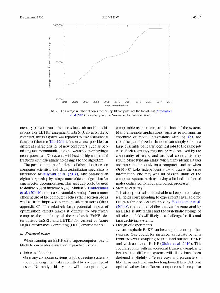
memory per core could also necessitate substantial modifi-

cations. For LETKF experiments with 5760 cores on the K

computer, the I/O system was reported to take a substantial

fraction of the time (Kunii 2014). It is, of course, possible that

different characteristics of new computers, such as per-

mitting faster communications between nodes or having a

more powerful I/O system, will lead to higher parallel

fractions with essentially no changes to the algorithm.

The positive impact of a close collaboration between

computer scientists and data assimilation specialists is

illustrated by Miyoshi et al. (2014), who obtained an

eightfold speedup by using amore efficient algorithm for

eigenvector decomposition. This speedup could be used

to doubleNens or increaseNmodel. Similarly, Houtekamer

et al. (2014b) report a substantial speedup from a more

efficient use of the computer caches (their section 3b) as

well as from improved communication patterns (their

appendix C). The relatively large potential impact of

optimization efforts makes it difficult to objectively

compare the suitability of the stochastic EnKF, de-

terministic EnSRF, and LETKF for current or future

High Performance Computing (HPC) environments.

d. Practical issues

When running an EnKF on a supercomputer, one is

likely to encounter a number of practical issues.

d Job class flooding.

On many computer systems, a job queueing system is

used to manage the tasks submitted by a wide range of

users. Normally, this system will attempt to give

comparable users a comparable share of the system.

Many ensemble applications, such as performing an

ensemble of model integrations with Eq. (5), are

trivial to parallelize in that one can simply submit a

large ensemble of nearly identical jobs to the same job

class. Such a strategy may not be well received by the

community of users, and artificial constraints may

result. More fundamentally, when many identical tasks

are run simultaneously on a computer, such as when

O(10000) tasks independently try to access the same

information, one may well hit physical limits of the

computer system, such as having a limited number of

nodes dedicated to input and output processes.d Storage capacity.

It is often practical and desirable to keep meteorolog-

ical fields corresponding to experiments available for

future reference. As explained by Houtekamer et al.

(2014b), the number of files that can be generated by

an EnKF is substantial and the systematic storage of

all relevant fields will likely be a challenge for disk and

tape archiving systems.d Design of experiments.

An atmospheric EnKF can be coupled to many other

systems. One could, for instance, anticipate benefits

from two-way coupling with a land surface EnKF

and with an ocean EnKF (Sluka et al. 2016). This

coupling comes with an additional technical complexity,

because the different systems will likely have been

designed in slightly different ways and parameters—

like the assimilationwindow length—will have different

optimal values for different components. It may also

FIG. 2. The average number of cores for the top 10 computers of the top500 list (Strohmaier

et al. 2015). For each year, the November list has been used.


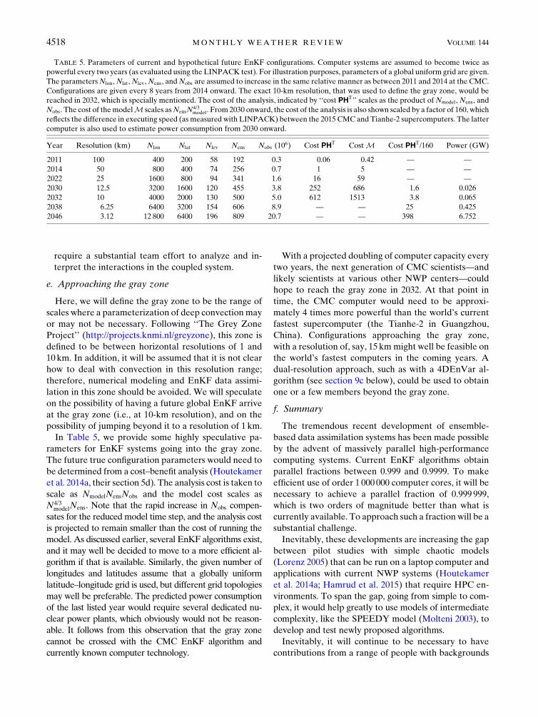
require a substantial team effort to analyze and in-

terpret the interactions in the coupled system.

e. Approaching the gray zone

Here, we will define the gray zone to be the range of

scales where a parameterization of deep convectionmay

or may not be necessary. Following ‘‘The Grey Zone

Project’’ (http://projects.knmi.nl/greyzone), this zone is

defined to be between horizontal resolutions of 1 and

10 km. In addition, it will be assumed that it is not clear

how to deal with convection in this resolution range;

therefore, numerical modeling and EnKF data assimi-

lation in this zone should be avoided. We will speculate

on the possibility of having a future global EnKF arrive

at the gray zone (i.e., at 10-km resolution), and on the

possibility of jumping beyond it to a resolution of 1 km.

In Table 5, we provide some highly speculative pa-

rameters for EnKF systems going into the gray zone.

The future true configuration parameters would need to

be determined from a cost–benefit analysis (Houtekamer

et al. 2014a, their section 5d). The analysis cost is taken to

scale as NmodelNensNobs and the model cost scales as

N4/3modelNens. Note that the rapid increase in Nobs compen-

sates for the reduced model time step, and the analysis cost

is projected to remain smaller than the cost of running the

model. As discussed earlier, several EnKF algorithms exist,

and it may well be decided to move to a more efficient al-

gorithm if that is available. Similarly, the given number of

longitudes and latitudes assume that a globally uniform

latitude–longitude grid is used, but different grid topologies

may well be preferable. The predicted power consumption

of the last listed year would require several dedicated nu-

clear power plants, which obviously would not be reason-

able. It follows from this observation that the gray zone

cannot be crossed with the CMC EnKF algorithm and

currently known computer technology.

With a projected doubling of computer capacity every

two years, the next generation of CMC scientists—and

likely scientists at various other NWP centers—could

hope to reach the gray zone in 2032. At that point in

time, the CMC computer would need to be approxi-

mately 4 times more powerful than the world’s current

fastest supercomputer (the Tianhe-2 in Guangzhou,

China). Configurations approaching the gray zone,

with a resolution of, say, 15 kmmight well be feasible on

the world’s fastest computers in the coming years. A

dual-resolution approach, such as with a 4DEnVar al-

gorithm (see section 9c below), could be used to obtain

one or a few members beyond the gray zone.

f. Summary

The tremendous recent development of ensemble-

based data assimilation systems has been made possible

by the advent of massively parallel high-performance

computing systems. Current EnKF algorithms obtain

parallel fractions between 0.999 and 0.9999. To make

efficient use of order 1 000 000 computer cores, it will be

necessary to achieve a parallel fraction of 0.999 999,

which is two orders of magnitude better than what is

currently available. To approach such a fraction will be a

substantial challenge.

Inevitably, these developments are increasing the gap

between pilot studies with simple chaotic models

(Lorenz 2005) that can be run on a laptop computer and

applications with current NWP systems (Houtekamer

et al. 2014a; Hamrud et al. 2015) that require HPC en-

vironments. To span the gap, going from simple to com-

plex, it would help greatly to use models of intermediate

complexity, like the SPEEDY model (Molteni 2003), to

develop and test newly proposed algorithms.

Inevitably, it will continue to be necessary to have

contributions from a range of people with backgrounds

TABLE 5. Parameters of current and hypothetical future EnKF configurations. Computer systems are assumed to become twice as

powerful every two years (as evaluated using the LINPACK test). For illustration purposes, parameters of a global uniform grid are given.

The parametersNlon,Nlat,Nlev,Nens, andNobs are assumed to increase in the same relative manner as between 2011 and 2014 at the CMC.

Configurations are given every 8 years from 2014 onward. The exact 10-km resolution, that was used to define the gray zone, would be

reached in 2032, which is specially mentioned. The cost of the analysis, indicated by ‘‘cost PHT’’ scales as the product of Nmodel, Nens, and

Nobs. The cost of themodelM scales asNensN4/3model. From 2030 onward, the cost of the analysis is also shown scaled by a factor of 160, which

reflects the difference in executing speed (as measured with LINPACK) between the 2015 CMC and Tianhe-2 supercomputers. The latter

computer is also used to estimate power consumption from 2030 onward.

Year Resolution (km) Nlon Nlat Nlev Nens Nobs (106) Cost PHT Cost M Cost PHT/160 Power (GW)

2011 100 400 200 58 192 0.3 0.06 0.42 — —

2014 50 800 400 74 256 0.7 1 5 — —

2022 25 1600 800 94 341 1.6 16 59 — —

2030 12.5 3200 1600 120 455 3.8 252 686 1.6 0.026

2032 10 4000 2000 130 500 5.0 612 1513 3.8 0.065

2038 6.25 6400 3200 154 606 8.9 — — 25 0.425

2046 3.12 12 800 6400 196 809 20.7 — — 398 6.752


http://projects.knmi.nl/greyzone

in the atmospheric, statistical, and computer sciences to

develop future assimilation systems.

9. Hybrids with variational and EnKF components

Hybrid systems now arise at operational centers, as

elements of emerging EnKF systems (e.g., Whitaker

et al. 2008; Houtekamer et al. 2014a) are being com-

bined with elements of well-functioning preexisting var-

iational assimilation systems (e.g., Parrish and Derber

1992; Rabier et al. 2000; Gauthier et al. 2007). In section

9a, the combination of static and ensemble-based co-

variances into a hybrid covariance matrix is discussed. It

is shown in section 9b how, in a traditional 4D-variational

framework, an extended control variable can de-

scribe the analysis increment as a sum of a static and

ensemble-based components. The 4DEnVar ensemble-

variational method, which is discussed in section 9c, is

similar but uses the EnKF ensemble, instead of line-

arized models, to estimate temporal covariances in the

assimilation window. In the hybrid gain algorithm

(section 9d), analysis increments from EnKF and var-

iational systems are simply weighted to obtain an

optimal analysis. A concluding discussion is provided in

section 9e.

a. Hybrid background error covariances

In the oldest form of hybrid, the ensemble covariance

P f is mixed (hybridized) with a static background error

covariance Ps, as proposed in Hamill and Snyder [2000,

their Eq. (4)]:

Phybrid

5bPs 1 (12b)P f . (33)

Here, the tuneable parameter b is used to obtain an

optimal weighting of the static and ensemble covari-

ances. The ensemble covariance P f has rank at most

Nens 2 1. In contrast, by virtue of its construction using a

diagonal matrix and a sequence of transformations

[Derber and Bouttier (1999), their Eq. (12)], the static

covariance Ps is normally full rank. The weighted sum

Phybrid of the low-rank ensemble covariances P f and the

full-rank static (climatological) background error co-

variances Ps is full rank. The use of the hybrid co-

variance will thus reduce the effects of sampling error

and rank deficiency (e.g., Wang et al. 2008; Zhang et al.

2009b; X. Wang et al. 2013; Kleist and Ide 2015a,b).

Static background error covariances are also often

used in an EnKF framework, in particular in the form of

additive inflation by drawing random perturbations

from a static background covariance [section 4a(1)]. In

that context, the two covariance terms are not averaged

but added and the static term is interpreted as a model

error covariance Q [Mitchell and Houtekamer (2000),

their Eq. (4)]:

P f 5Pp 1Q , (34)

where Pp is prediction error obtained with a perfect

model. In the ensemble implementation with Eq. (22),

the addition of model error may sample new directions

in phase space, but the rank of the Nens-member en-

semble cannot increase beyond Nens 2 1 (Meng and

Zhang 2008a).

At an operational center, one could well decide to use

only a single static covariancematrixPs 5Q for both the

weighted average of the hybrid [Eq. (33)] and the model

error simulation in the EnKF [Eq. (34)]. Substituting

Eq. (34) into Eq. (33), we find that

Phybrid

5 (12b)Pp 1Q . (35)

Comparing Eqs. (34) and (35), it is seen that the hybrid

matrix Phybrid gives a reduced weight to flow-dependent

covariances Pp as compared to the matrix P f of the

EnKF. Equivalently, it can be stated that the model

error sampling is relatively more important in the hybrid

systemwhere it also serves toward further regularization

of the rank problem.

In the EnKF framework, the addition of perturbations

generated from static error covariances may also be

done at the stage of the posterior covariance (Hunt et al.

2004; Houtekamer and Mitchell 2005) allowing the

forecast model M, to evolve these perturbations to the

subsequent assimilation window.

b. E4DVar with the a control variable

With the a control variable approach proposed by

Lorenc (2003), the cost function J in the hybrid ensemble-

variational system (EnVar) can be expressed as

J(v1,a)5

1

2vT1 v1 1

1

2aT

0B@

C 0

⋯

0 C

1CA21

a1 Jo5

J(v1, v

2)5

1

2vT1 v1 1

1

2vT2 v2 1 J

o. (36)

Here, C is a localizing covariance and a contains

smoothly varying fields of weights for the ensemble of

background error fields. The background term in the

cost function [Eq. (36)] is then computed as a function of

the traditional preconditioning control variable v1(Barker et al. 2012) and the ensemble-based (a) control

variable v2 (Lorenc 2003). The cost of the distance to the

observations is measured using Jo as usual in variational

minimization.


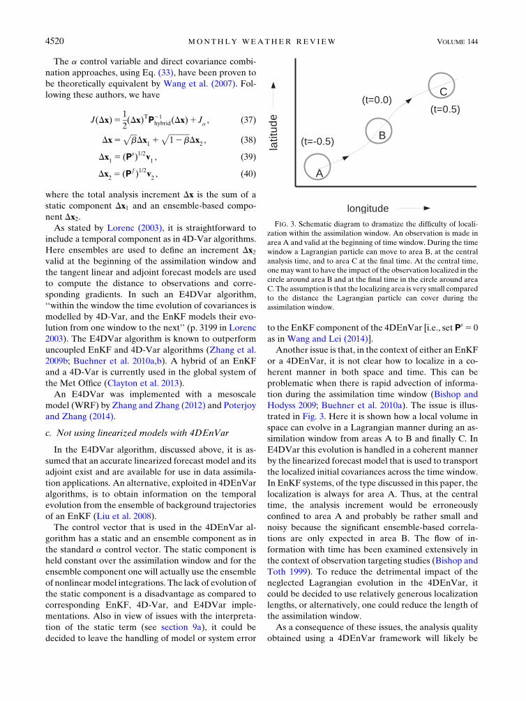
The a control variable and direct covariance combi-

nation approaches, using Eq. (33), have been proven to

be theoretically equivalent by Wang et al. (2007). Fol-

lowing these authors, we have

J(Dx)51

2(Dx)TP21

hybrid(Dx)1 Jo, (37)

Dx5ffiffiffib

pDx

11

ffiffiffiffiffiffiffiffiffiffiffi12b

pDx

2, (38)

Dx15 (Ps)1/2v

1, (39)

Dx25 (P f )1/2v

2, (40)

where the total analysis increment Dx is the sum of a

static component Dx1 and an ensemble-based compo-

nent Dx2.As stated by Lorenc (2003), it is straightforward to

include a temporal component as in 4D-Var algorithms.

Here ensembles are used to define an increment Dx2valid at the beginning of the assimilation window and

the tangent linear and adjoint forecast models are used

to compute the distance to observations and corre-

sponding gradients. In such an E4DVar algorithm,

‘‘within the window the time evolution of covariances is

modelled by 4D-Var, and the EnKF models their evo-

lution from one window to the next’’ (p. 3199 in Lorenc

2003). The E4DVar algorithm is known to outperform

uncoupled EnKF and 4D-Var algorithms (Zhang et al.

2009b; Buehner et al. 2010a,b). A hybrid of an EnKF

and a 4D-Var is currently used in the global system of

the Met Office (Clayton et al. 2013).

An E4DVar was implemented with a mesoscale

model (WRF) by Zhang and Zhang (2012) and Poterjoy

and Zhang (2014).

c. Not using linearized models with 4DEnVar

In the E4DVar algorithm, discussed above, it is as-

sumed that an accurate linearized forecast model and its

adjoint exist and are available for use in data assimila-

tion applications. An alternative, exploited in 4DEnVar

algorithms, is to obtain information on the temporal

evolution from the ensemble of background trajectories

of an EnKF (Liu et al. 2008).

The control vector that is used in the 4DEnVar al-

gorithm has a static and an ensemble component as in

the standard a control vector. The static component is

held constant over the assimilation window and for the

ensemble component one will actually use the ensemble

of nonlinearmodel integrations. The lack of evolution of

the static component is a disadvantage as compared to

corresponding EnKF, 4D-Var, and E4DVar imple-

mentations. Also in view of issues with the interpreta-

tion of the static term (see section 9a), it could be

decided to leave the handling of model or system error

to the EnKF component of the 4DEnVar [i.e., set Ps 5 0

as in Wang and Lei (2014)].

Another issue is that, in the context of either an EnKF

or a 4DEnVar, it is not clear how to localize in a co-

herent manner in both space and time. This can be

problematic when there is rapid advection of informa-

tion during the assimilation time window (Bishop and

Hodyss 2009; Buehner et al. 2010a). The issue is illus-

trated in Fig. 3. Here it is shown how a local volume in

space can evolve in a Lagrangian manner during an as-

similation window from areas A to B and finally C. In

E4DVar this evolution is handled in a coherent manner

by the linearized forecast model that is used to transport

the localized initial covariances across the time window.

In EnKF systems, of the type discussed in this paper, the

localization is always for area A. Thus, at the central

time, the analysis increment would be erroneously

confined to area A and probably be rather small and

noisy because the significant ensemble-based correla-

tions are only expected in area B. The flow of in-

formation with time has been examined extensively in

the context of observation targeting studies (Bishop and

Toth 1999). To reduce the detrimental impact of the

neglected Lagrangian evolution in the 4DEnVar, it

could be decided to use relatively generous localization

lengths, or alternatively, one could reduce the length of

the assimilation window.

As a consequence of these issues, the analysis quality

obtained using a 4DEnVar framework will likely be

FIG. 3. Schematic diagram to dramatize the difficulty of locali-

zation within the assimilation window. An observation is made in

area A and valid at the beginning of time window. During the time

window a Lagrangian particle can move to area B, at the central

analysis time, and to area C at the final time. At the central time,

onemaywant to have the impact of the observation localized in the

circle around area B and at the final time in the circle around area

C. The assumption is that the localizing area is very small compared

to the distance the Lagrangian particle can cover during the

assimilation window.


inferior to the quality obtained with a E4DVar system

(Clayton et al. 2013; Lorenc et al. 2015; Poterjoy and

Zhang 2015, 2016).

The first operational implementation of a 4D ensemble-

variational (4DEnVar) algorithm occurred at the CMC

where, since November 2014, it is used for the determin-

istic global (Buehner et al. 2015) and regional (Caron et al.

2015) analyses. Currently, NCEP is also in the process of

upgrading to 4DEnVar from the current 3D com-

posite system (3DEnVar) (D. Kleist 2015, personal

communication).

d. The hybrid gain algorithm

So far, it has been assumed that the EnKF system and

the variational solver have each been developed fairly

independently to a comparable level of quality such that

it becomes advantageous for an operational center to

create a hybrid system.

Working in the context of the Lorenz 40-component

model, Penny (2014) proposed to hybridize the gain

matrices of a variational and an EnKF assimilation

system by weighting the analyses from the two compo-

nent systems (which here were a 3D-Var and an

LETKF). This is equivalent to recentering the EnKF

mean analysis xa and the deterministic analysis xadet using

the following:

xacentered 5 gxa 1 (12g)xadet . (41)

Here g is some tuneable constant that depends on the

relative quality of the two systems. The algorithm is il-

lustrated in Fig. 4 of Bonavita et al. (2015).

The approach has been explored further at NCEP in

the context of a global ocean data assimilation system

(Penny et al. 2015). Similar to what is seen with themore

common hybrids, which combine the ensemble and

background error covariances (section 9a), the hybrid

gain approach provides benefit when the ensemble size

is small, because the analysis increment is not restricted

to the space spanned by ensemble members. Because of

the use of a climatological covariance in the variational

component, it also improves the analysis in regions

where observations are sparse.

Bonavita et al. (2015) applied Penny’s hybrid gain

algorithm to hybridize the gain matrices from in-

dependent EnKF and 4D-Var systems. They found that

the hybrid gain system outperformed its two component

systems (i.e., EnKF and static B 4D-Var). It was also

competitive with a reduced-resolution version of the

hybrid 4D-Var–EDA system used operationally at

ECMWF. That operational system uses an ensemble of

independent adjoint-based 4D-Var analyses, where the

ensemble is used to estimate flow-dependent error

variances (Bonavita et al. 2012). A practical advantage

of the hybrid gain approach is that it permits indepen-

dent parallel development of EnKF and variational

systems to have a beneficial impact on the resulting

hybrid system (Bonavita et al. 2015).

e. Open issues and recommendations

Generally speaking, among hybrid algorithms, it

would seem that the E4DVar method is superior to the

4DEnVar methods. This may be mostly due to the lat-

ter’s use of a static term in the hybrid background error

covariances and to the difficulty of localizing covari-

ances over a long window. Possibly, removing the static

term and using less localization with larger ensembles

and a shorter assimilation window would invert the sit-

uation with now superior results for the 4DEnVar due to

its use of a nonlinear model to transport covariance in-

formation over the assimilation window. The use of a

4DEnVar algorithm may also promote faster model

development because with this approach accurate line-

arized models would no longer be required by the data

assimilation systems.

Beyond discipline, it is not clear if there is a general

development strategy that will minimize configuration

differences between the components of the hybrid. An

extreme solution would be to abandon the hybrid and

either (i) obtain all required analyses from the direct

solver of the EnKF or (ii) obtain all required analyses

from an ensemble of variational solutions. Current com-

parisons of computational cost would likely favor (i), but

this situation could change if efficient parallel algorithms

for ensemble minimization become available. On the

other hand, it would seem from in particular the expe-

rience with the assimilation of radiance observations

that higher-quality results can be obtained with (ii).

There is, however, no generally accepted explanation

for this apparently higher quality.

It is hard to predict how the quality of the component

variational and EnKF systems will evolve in the future.

For the foreseeable future, the hybrid gain algorithm

can serve as a simple and practical method to combine

desirable aspects of both families of algorithms.

10. Summary and discussion

In recent years, there has been a flurry of activity with

respect to global (e.g., Table 1) and regional EnKF

systems. Houtekamer et al. (2014a) see a virtuous cycle,

in which increasingly powerful computer systems, an

improved sampling of errors with larger ensembles,

more active higher-resolution dynamics, and more re-

alistic models with less systematic problems all conspire

toward an ever higher-quality approximation of the


underlying Kalman filter. Nevertheless, as we will

summarize below, the burgeoning field of ensemble-

based data assimilation is full of unresolved issues.

a. Stochastic or deterministic filters

Perhaps the main split in the EnKF community is with

respect to the use of a stochastic or a deterministic

algorithm.

With the stochastic algorithm, we have the perhaps

naive hope that eventually we will manage to identify all

themajor sources of error (Table 4) and find appropriate

ways to sample these in the Monte Carlo framework. In

this view, localization deals only with the rank problem

associated with a small ensemble size and additive co-

variance inflation is a stand-in for (to be developed)

algorithms that will account for, and sample, specific

weaknesses in the system.

The deterministic algorithm is more pragmatic. The

aim is to obtain an accurate best estimate using a mini-

mum number of ensemble members and, to this end, it is

better to avoid randomperturbations to observations. If,

for some reason, the ensemble statistics are not reliable

they can be corrected by an appropriate adaptive algo-

rithm. This can be a localization or relaxation algorithm

of which the parameters are tuned to minimize analysis

and prediction error.

The current split between stochastic algorithms with

cross validation and deterministic algorithms with re-

laxation methods could possibly be resolved if cross vali-

dation could be implemented in deterministic algorithms.

b. The nature of system error

Properly accounting for estimated uncertainties of the

observations and letting errors evolve and grow with the

dynamics of the model, one arrives at estimated error

levels for the analysis or background that are much too

optimistic. Ideally, the missing error sources would be

identified and included in the Monte Carlo error simu-

lation of the EnKF system. To have a comprehensive

quantitative list of the weaknesses in an NWP system

would be of immense value for the realism of the EnKF

system, and it would greatly facilitate work toward im-

provement of the NWP system itself. The task, however,

is daunting. Since the number of possible issues in the

system is huge, it may prove easier to find a needle in a

haystack with O(100) dimensions (Tarantola 2006).

Lacking a comprehensive list, a variety of bulk methods

has been developed to maintain a realistic amount of

spread in an EnKF system (section 4). Simple methods for

covariance inflation (section 4a), like relaxation to prior,

additive covariance inflation or a combination of these two

methods, provide generally satisfying reliability and it has

so far proven difficult to obtain better results with more

sophisticated methods. Some improvement has, however,

been observed from using multiple physical parameteri-

zations [section 4c(2)] to sample the ‘‘model error’’ com-

ponent of the total ‘‘system error.’’ There is currently no

consensus in the community on how to move toward

schemes that comprehensively sample model error

[section 4c(3)]. Options include the development of

either a complete set of stochastic parameterizations,

covering all parameterized processes, or a comprehensive

set of possible deterministic parameterizations.

c. Going beyond the synoptic scales

The global EnKF systems originated in environments

appropriate for synoptic-scale data assimilation. At

these scales, the temporal evolution is slow, fairly well

described by the numerical model, and it is sufficient to

do the analysis every 6h. Covariance localization can be

done in various ways, but must use relatively broad

functions—O(1000) km in the horizontal—to preserve

geostrophic balance in the analysis increments. Tradi-

tional balancing methods, like the digital filter, can be

used to filter any undesired gravity waves.

Going to shorter temporal scales and shorter assimi-

lation window lengths, it would seem advantageous to

move to the incremental analysis update (IAU) pro-

cedure, in which analysis increments are gradually

added as a forcing to a continuous model integration.

When the window length reduces, the IAU will, how-

ever, start filtering shorter temporal scales and may

become less effective as a balancing method. Perhaps,

we need to return to balancing methods that act on ten-

dencies observed at the initial model time step (Hamrud

et al. 2015).

Adding shorter horizontal scales creates a difficult

superposition of large-scale, almost geostrophic, dy-

namics and small-scale intermittent convective activity.

Traditional localization methods, with prescribed

smooth functions, cannot deal with this situation unless

the ensemble is made large enough that no localization is

required for small scales. Miyoshi and Kondo (2013)

propose to use a multiscale localization approach, where a

regular small-scale analysis obtained with severe localiza-

tion is augmented with remote larger-scale components

obtained from analyses using smoothed perturbations.

Alternatively, one may have to use a flow-dependent and

observation-type-dependent localization procedure. For

data assimilation in hurricane environments, successive

covariance localization (SCL; Zhang et al. 2009a) permits

zooming in on interesting features in the well-observed

central area. In thunderstorm environments, it is common

to use observation-type-dependent localization (Meng and

Zhang 2008a; Snook et al. 2015). In particular in the con-

text of sequential algorithms, it could appear that one is


free to localize each observation with specific criteria. A

caveat is that interaction between the sequential process-

ing and the localization can lead to instability (Nerger

2015). How to best localize the information from multiple

observations is an unresolved problem [section 3e(3)].

There is a significant user need for accurate forecasts

of severe convective storms. Such systems are often

observed at high temporal and spatial resolution with

dual-polarization radar. Likely, for a routine high-quality

EnKFconvective-scale analysis onewouldneedO(1000)-m

horizontal resolution, an accurate higher-moment micro-

physics scheme, and an accurate description of observa-

tional errors. In addition, one will have to deal with

sporadic irregular dynamics, non-Gaussian error dynam-

ics, and many additional, mostly unobserved, model vari-

ables. It is too early to tell if the problem can successfully

be addressed in the context of an EnKF.

d. Satellite observations

Global EnKF systems now routinely assimilate a fair

amount of radiance observations with some success.

Although there are few corresponding studies, it does

nevertheless seem that their impact is not as large and

critical to good performance as in corresponding varia-

tional systems. Possible explanations are the follow-

ing: suboptimal covariance localization, a difficulty of

the EnKF to deal with dense observation sets, im-

perfect bias removal, and neglected observation-error

correlations.

It would be important for the EnKF community to

learn how to make optimal use of all available obser-

vation types. A systematic analysis of many of the issues

relating to the assimilation of radiance observations

could be done in the context of an observing system

simulation experiment (OSSE).

e. Hybrid systems

In hybrid systems, one tries to combine components of

existing EnKF and variational analysis systems to

obtain a better coupled system. Similar to the experi-

ence with multimodel ensembles like the North Amer-

ican Ensemble Forecast System (NAEFS; Candille

2009), a substantial improvement is generally associated

with the combination of two fairly independent systems

of similar quality. This has been shown by Bonavita et al.

(2015) in the implementation of the gain hybrid of the

4D-Var and LETKF assimilation systems.

A difficulty with a hybrid system is that it requires a

sustained investment and development for the two

component systems as well as for the combined sys-

tem. It is not clear that the operational centers can

and will support a hybrid system for an extended

period of time.

f. Future of the EnKF

It would seem that EnKF systems can continue to

benefit from improvements in computational platforms

for some time to come. The use of notably higher reso-

lution and more members should fairly easily translate

into higher analysis quality. It would seem possible, in

the future, to have global EnKF configurations that

approach the gray zone (a horizontal resolution of ap-

proximately 10 km). In this endeavor, it will likely be of

value that a moderately large variety of ensemble-based

data assimilation systems, using different parallelization

and (due to their fundamental impact on computational

efficiency) localization strategies, exists at operational

centers.

Improved boundary conditions, including a reason-

able estimate of uncertainty, could be provided by

coupling of an atmospheric EnKF with similar systems

for the ocean, the ice, the land surface, chemical con-

stituents, etc. In principle, it is possible to have a unique

data assimilation application that uses all observations

to estimate the state vector of all component systems

using a single gain matrix (Tardif et al. 2015; Sluka et al.

2016). Challenges for such coupled assimilation systems

come from different spatial and temporal scales in the

component systems, from possibly weak and, therefore,

hard to estimate correlations across boundaries and

from the likely complex dynamics of the coupled system.

It may also be possible to alleviate some of the con-

straints that seem to be imposed by the Kalman filter

framework. For instance, Lien et al. (2013, 2016a,b) re-

cently proposed several ways of addressing the non-

Gaussian distributions of precipitation, including the use

of a Gaussian transformation of variables, and the as-

similation of both zero precipitation and nonzero pre-

cipitation observations.

In particular because of the huge electricity re-

quirement, it does not appear possible to have an EnKF

configuration that functions beyond the gray zone, at a

horizontal resolution of 1 km or higher, with current

computer technology. For global convection-resolving

data assimilation, it may be necessary to use dual-

resolution configurations.

Acknowledgments.This paper started as a summary of

the material presented and discussed at the Sixth EnKF

Workshop that was held 18–22 May 2014 near Buffalo,

New York, and we want to thank all workshop partici-

pants. We thank Herschel Mitchell and Jonathan

Poterjoy for internal reviews with many valuable sug-

gestions. We thank Luc Fillion for, notably, discussions

regarding balance and regional data assimilation. We

thank the reviewers Geir Evensen and Eugenia Kalnay,


as well as an anonymous reviewer, for numerous valu-

able suggestions that helped us to improve the manu-

script. FZ is partially supported by NSF Grant 1305798,

Office of Naval Research Grant N000140910526, and

NASA Grant NNX12AJ79G.

APPENDIX A

Types of Filter Divergence

In filter divergence, the best estimate provided by the

EnKF becomes disconnected from reality. In classical

filter divergence, well known from Kalman filter sys-

tems, the ensemble spread becomes much too small. An

EnKF can also suffer from catastrophic filter divergence

in which the ensemble spread becomes very large.

a. Classical filter divergence

It is well known that the Kalman filter can display

unstable behavior (Lewis et al. 2006, their section 28.4;

Snyder 2015, his section 3.5.4). The following issues can

play a role in filter divergence: model bias and errors,

errors in specified statistics, round-off errors, and non-

linearity in the system. A symptom of the divergence is a

high-condition number of the matrix Pf . A standard

approach for dealing with this problem is to reformulate

the algorithm using square root matrices (Lewis et al.

2006, their section 28.4) or to add a high-rank system

noise (Fitzgerald 1971). Similarly, in modern atmo-

spheric applications of the EnKF, the rank problem that

is associated with small ensemble sizes will naturally

lead to a high or even infinite condition number (section

3d). Covariance localization and the addition of system

error are often used to protect against the associated

filter divergence (Whitaker andHamill 2002, see revised

Fig. 3 in the corrigendum to their article). Note, how-

ever, that covariance localization, in combination with a

sequential algorithm, can also be a cause of filter di-

vergence (section 7b above; Nerger 2015). In environ-

ments with stable dynamics—or no dynamics at all as in

the case of parameter estimation (Aksoy et al. 2006)—

there may also be issues, and it is a good practice to

always verify that the estimated variances of the

background error remain significant.

b. Catastrophic filter divergence

In the EnKF context, there are what would seem to be

new types of instability (Houtekamer andMitchell 2005,

their section 3b; Kelly et al. 2015). The issue here is that

the ensemble spread becomes very large. This will lead

to large-amplitude analysis increments and, when un-

checked, can lead to initial conditions that can no longer

be handled by the numerical model.

In the case of observations that are only weakly cor-

related with the model state, the estimation noise can be

larger than the signal and the analysis can be less accu-

rate than the background for some variables. When a

cross-validation procedure is used, the EnKF is ‘‘aware’’

of this situation and the analysis spread will exceed the

spread in the background (Houtekamer and Mitchell

2005, their section 3b). This increased spread subsequently

enables larger analysis increments when subsequent sets of

similar observations are assimilated in the sequential

analysis algorithm. When the number of observations is

large, this divergence can act very quickly. This instability

can be reduced or controlled notably by using larger en-

sembles and more severe covariance localization.

In the example by Kelly et al. (2015), the observation

is perpendicular to the ensemble subspace and the cat-

astrophic blow-up results as an interplay between the

numerical model and the forward operator. In this case,

additive covariance inflation can stabilize the filter.

Finally, we note once more that filter divergence can

also result from the use of multiplicative inflation in

data-sparse areas (Anderson 2009) and potentially from

other methods to inflate ensemble spread such as the

addition of physical tendency perturbations.

Since, as we have seen, both large and small ensemble

spread can cause filter divergence, EnKF systems inten-

ded for operational applications have to be designed and

tested with great care.

APPENDIX B

Systems Available for Download

Most ensemble Kalman filter algorithms are concep-

tually fairly simply. However, to obtain good perfor-

mance on a supercomputer with a true forecasting

model and a variety of observation types represents a

major effort. Starting essentially from scratch, but em-

bedded in an operational environment, Drs. Houtekamer

and Mitchell and coworkers needed approximately

10 years to arrive at their first operational implementa-

tion (Houtekamer et al. 2005). Similarly, the EnSRF,

which had been developed originally at NCAR, has been

implemented for operational use at NCEP (Whitaker

et al. 2008) and for research use at ECMWF.Operational

centers, with no experience in ensemble-based data as-

similation, can likely benefit from the experience and

code developed at other centers. Here wewant to refer to

three specific efforts to make ensemble-based data as-

similation available to a larger group of users.

The Data Assimilation Research Testbed (DART)

is a community facility (Anderson et al. 2009) for

ensemble-based data assimilation that is developed and


supported by the National Center for Atmospheric

Research (NCAR). It includes many models ranging

from very simple to fairly complex and has a large com-

munity of users. The code is accessible using subversion

from a central code repository (http://www.image.ucar.

edu/DAReS/DART/). First results in complex environ-

ments can reportedly be obtained in a few months.

The source code of aWRF-basedEnKF system (Zhang

et al. 2009a, 2011;Weng andZhang 2012), which has been

continuously developed at The Pennsylvania State Uni-

versity, and is used for experimental real-time convection-

permitting hurricane analysis and prediction, can be

freely downloaded online at http://adapt.psu.edu/index.

php?loc5outreach.

The source code of the LETKF (Hunt et al. 2007),

which has originally been developed at the University of

Maryland, has been made available for download by

T. Miyoshi at https://code.google.com/p/miyoshi. The

LETKF has a large, rather loose, community of users.

The above initiatives will facilitate the work toward

obtaining initial results. Beyond that, a substantial amount

of experimentation will likely be required to arrive at a

robust system with a satisfying quality.

REFERENCES

Aksoy, A., F. Zhang, and J.W. Nielsen-Gammon, 2006: Ensemble-

based simultaneous state and parameter estimation in a two-

dimensional sea-breeze model. Mon. Wea. Rev., 134, 2951–2970,doi:10.1175/MWR3224.1.

——, D. C. Dowell, and C. Snyder, 2009: A multicase comparative

assessment of the ensemble Kalman filter for assimilation of

radar observations. Part I: Storm-scale analyses. Mon. Wea.

Rev., 137, 1805–1824, doi:10.1175/2008MWR2691.1.

——,——, and——, 2010: A multicase comparative assessment of

the ensemble Kalman filter for assimilation of radar obser-

vations. Part II: Short-range ensemble forecasts. Mon. Wea.

Rev., 138, 1273–1292, doi:10.1175/2009MWR3086.1.

——, S. D. Aberson, T. Vukicevic, K. J. Sellwood, S. Lorsolo, and

X. Zhang, 2013: Assimilation of high-resolution tropical cy-

clone observations with an ensemble Kalman filter using

NOAA/AOML/HRD’s HEDAS: Evaluation of the 2008–11

vortex-scale analyses. Mon. Wea. Rev., 141, 1842–1865,

doi:10.1175/MWR-D-12-00194.1.

Albers, S. C., J. A. McGinley, D. L. Birkenheuer, and J. R. Smart,

1996: The Local Analysis and Prediction System (LAPS):

Analysis of clouds, precipitation, and temperature. Wea. Fore-

casting, 11, 273–287, doi:10.1175/1520-0434(1996)011,0273:

TLAAPS.2.0.CO;2.

Amezcua, J., K. Ide, E. Kalnay, and S. Reich, 2014: Ensemble

transform Kalman–Bucy filters. Quart. J. Roy. Meteor. Soc.,

140, 995–1004, doi:10.1002/qj.2186.Anderson, J. L., 2001: An ensemble adjustment Kalman filter for

data assimilation. Mon. Wea. Rev., 129, 2884–2903, doi:10.1175/

1520-0493(2001)129,2884:AEAKFF.2.0.CO;2.

——, 2003: A local least squares framework for ensemble

filtering. Mon. Wea. Rev., 131, 634–642, doi:10.1175/

1520-0493(2003)131,0634:ALLSFF.2.0.CO;2.

——, 2007: Exploring the need for localization in ensemble data

assimilation using a hierarchical ensemble filter. Physica D,

230, 99–111, doi:10.1016/j.physd.2006.02.011.

——, 2009: Spatially and temporally varying adaptive covariance

inflation for ensemble filters. Tellus, 61A, 72–83, doi:10.1111/

j.1600-0870.2008.00361.x.

——, 2012: Localization and sampling error correction in ensemble

Kalman filter data assimilation. Mon. Wea. Rev., 140, 2359–

2371, doi:10.1175/MWR-D-11-00013.1.

——, 2016: Reducing correlation sampling error in ensemble

Kalman filter data assimilation.Mon.Wea. Rev., 144, 913–925,

doi:10.1175/MWR-D-15-0052.1.

——, and S. L. Anderson, 1999: AMonte Carlo implementation of

the nonlinear filtering problem to produce ensemble assimila-

tions and forecasts.Mon.Wea. Rev., 127, 2741–2758, doi:10.1175/

1520-0493(1999)127,2741:AMCIOT.2.0.CO;2.

——, T. Hoar, K. Raeder, H. Liu, N. Collins, R. Torn, and

A. Avellano, 2009: The Data Assimilation Research Testbed:

A community facility.Bull. Amer.Meteor. Soc., 90, 1283–1296,

doi:10.1175/2009BAMS2618.1.

Annan, J. D., 2004: On the orthogonality of bred vectors. Mon.

Wea. Rev., 132, 843–849, doi:10.1175/1520-0493(2004)132,0843:

OTOOBV.2.0.CO;2.

——, J. C. Hargreaves, N. R. Edwards, and R. Marsh, 2005: Pa-

rameter estimation in an intermediate complexity earth sys-

temmodel using an ensemble Kalman filter.OceanModell., 8,

135–154, doi:10.1016/j.ocemod.2003.12.004.

Aravéquia, J. A., I. Szunyogh, E. J. Fertig, E. Kalnay, D. Kuhl, and

E. J. Kostelich, 2011: Evaluation of a strategy for the assimi-

lation of satellite radiance observations with the local ensemble

transform Kalman filter. Mon. Wea. Rev., 139, 1932–1951,

doi:10.1175/2010MWR3515.1.

Ballish, B., X. Cao, E. Kalnay, and M. Kanamitsu, 1992: In-

cremental nonlinear normal-mode initialization. Mon. Wea.

Rev., 120, 1723–1734, doi:10.1175/1520-0493(1992)120,1723:

INNMI.2.0.CO;2.

Barker, D. M., 2005: Southern high-latitude ensemble data assim-

ilation in theAntarticmesoscale prediction system.Mon.Wea.

Rev., 133, 3431–3449, doi:10.1175/MWR3042.1.

——, andCoauthors, 2012: TheWeatherResearch and Forecasting

Model’s Community Variational/Ensemble Data Assimila-

tion System: WRFDA. Bull. Amer. Meteor. Soc., 93, 831–843,

doi:10.1175/BAMS-D-11-00167.1.

Bergemann, K., and S. Reich, 2010: A mollified ensemble Kalman

filter.Quart. J. Roy. Meteor. Soc., 136, 1636–1643, doi:10.1002/

qj.672.

Berner, J., G. J. Shutts, M. Leutbecher, and T. N. Palmer, 2009: A

spectral stochastic kinetic energy backscatter scheme and its

impact on flow-dependent predictability in the ECMWF

ensemble prediction system. J. Atmos. Sci., 66, 603–626,

doi:10.1175/2008JAS2677.1.

Bishop, C. H., and Z. Toth, 1999: Ensemble transformation and

adaptive observations. J. Atmos. Sci., 56, 1748–1765, doi:10.1175/

1520-0469(1999)056,1748:ETAAO.2.0.CO;2.

——, and D. Hodyss, 2009: Ensemble covariances adaptively lo-

calized with ECO-RAP. Part 1: Tests on simple error models.

Tellus, 61A, 84–96, doi:10.1111/j.1600-0870.2008.00371.x.

——, B. J. Etherton, and S. J. Majumdar, 2001: Adaptive sampling

with the ensemble transform Kalman filter. Part I: Theo-

retical aspects. Mon. Wea. Rev., 129, 420–436, doi:10.1175/

1520-0493(2001)129,0420:ASWTET.2.0.CO;2.

Bloom, S. C., L. L. Takacs, A. M. da Silva, and D. Ledvina, 1996:

Data assimilation using incremental analysis updates. Mon.


http://www.image.ucar.edu/DAReS/DART/

http://www.image.ucar.edu/DAReS/DART/

http://adapt.psu.edu/index.php?loc=outreach

http://adapt.psu.edu/index.php?loc=outreach

https://code.google.com/p/miyoshi

http://dx.doi.org/10.1175/MWR3224.1

http://dx.doi.org/10.1175/2008MWR2691.1


http://dx.doi.org/10.1175/MWR-D-12-00194.1

http://dx.doi.org/10.1175/1520-0434(1996)011<0273:TLAAPS>2.0.CO;2

http://dx.doi.org/10.1175/1520-0434(1996)011<0273:TLAAPS>2.0.CO;2

http://dx.doi.org/10.1002/qj.2186

http://dx.doi.org/10.1175/1520-0493(2001)129<2884:AEAKFF>2.0.CO;2

http://dx.doi.org/10.1175/1520-0493(2001)129<2884:AEAKFF>2.0.CO;2

http://dx.doi.org/10.1175/1520-0493(2003)131<0634:ALLSFF>2.0.CO;2

http://dx.doi.org/10.1175/1520-0493(2003)131<0634:ALLSFF>2.0.CO;2

http://dx.doi.org/10.1016/j.physd.2006.02.011

http://dx.doi.org/10.1111/j.1600-0870.2008.00361.x

http://dx.doi.org/10.1111/j.1600-0870.2008.00361.x



http://dx.doi.org/10.1175/1520-0493(1999)127<2741:AMCIOT>2.0.CO;2

http://dx.doi.org/10.1175/1520-0493(1999)127<2741:AMCIOT>2.0.CO;2

http://dx.doi.org/10.1175/2009BAMS2618.1

http://dx.doi.org/10.1175/1520-0493(2004)132<0843:OTOOBV>2.0.CO;2

http://dx.doi.org/10.1175/1520-0493(2004)132<0843:OTOOBV>2.0.CO;2

http://dx.doi.org/10.1016/j.ocemod.2003.12.004


http://dx.doi.org/10.1175/1520-0493(1992)120<1723:INNMI>2.0.CO;2

http://dx.doi.org/10.1175/1520-0493(1992)120<1723:INNMI>2.0.CO;2


http://dx.doi.org/10.1175/BAMS-D-11-00167.1



http://dx.doi.org/10.1175/2008JAS2677.1

http://dx.doi.org/10.1175/1520-0469(1999)056<1748:ETAAO>2.0.CO;2

http://dx.doi.org/10.1175/1520-0469(1999)056<1748:ETAAO>2.0.CO;2

http://dx.doi.org/10.1111/j.1600-0870.2008.00371.x

http://dx.doi.org/10.1175/1520-0493(2001)129<0420:ASWTET>2.0.CO;2

http://dx.doi.org/10.1175/1520-0493(2001)129<0420:ASWTET>2.0.CO;2

Wea. Rev., 124, 1256–1271, doi:10.1175/1520-0493(1996)124,1256:

DAUIAU.2.0.CO;2.

Bonavita, M., 2011: Impact and diagnosis of model error in the

ECMWF ensemble of data assimilations. Proc. ECMWF

Workshop on Representing Model Uncertainty and Error in

Numerical Weather and Climate Prediction Models, Shinfield

Park, Reading, United Kingdom, ECMWF, 303–318.

——, L. Torrisi, and F.Marcucci, 2010: Ensemble data assimilation

with the CNMCA regional forecasting system. Quart. J. Roy.

Meteor. Soc., 136, 132–145, doi:10.1002/qj.553.

——, L. Isaksen, and E. Hólm, 2012: On the use of EDA back-

ground error variances in the ECMWF 4D-Var.Quart. J. Roy.

Meteor. Soc., 138, 1540–1559, doi:10.1002/qj.1899.

——, M. Hamrud, and L. Isaksen, 2015: EnKF and hybrid gain

ensemble data assimilation. Part II: EnKF and hybrid gain

results. Mon. Wea. Rev., 143, 4865–4882, doi:10.1175/

MWR-D-15-0071.1.

——, E. Hólm, L. Isaksen, and M. Fisher, 2016: The evolution of

the ECMWF hybrid data assimilation system. Quart. J. Roy.

Meteor. Soc., 142, 287–303, doi:10.1002/qj.2652.Bormann, N., and P. Bauer, 2010: Estimates of spatial and in-

terchannel observation-error characteristics for current sounder

radiances for numerical weather prediction. I: Methods and ap-

plication toATOVS data.Quart. J. Roy.Meteor. Soc., 136, 1036–

1050, doi:10.1002/qj.616.

Bowler, N. E., A. Arribas, K. R. Mylne, K. B. Robertson, and S. E.

Beare, 2008: The MOGREPS short-range ensemble pre-

diction system. Quart. J. Roy. Meteor. Soc., 134, 703–722,

doi:10.1002/qj.234.

Brankart, J.-M., C. Ubelmann, C.-E. Testut, E. Cosme, P. Brasseur,

and J. Verron, 2009: Efficient parameterization of the obser-

vation error covariance matrix for square root or ensemble

Kalman filters: Application to ocean altimetry. Mon. Wea.

Rev., 137, 1908–1927, doi:10.1175/2008MWR2693.1.

Buehner, M., 2012: Evaluation of a spatial/spectral covariance lo-

calization approach for atmospheric data assimilation. Mon.

Wea. Rev., 140, 617–636, doi:10.1175/MWR-D-10-05052.1.

——, P. L. Houtekamer, C. Charette, H. L. Mitchell, and B. He,

2010a: Intercomparison of variational data assimilation and

the ensembleKalman filter for global deterministic NWP. Part

I: Description and single-observation experiments.Mon. Wea.

Rev., 138, 1550–1566, doi:10.1175/2009MWR3157.1.

——, ——, ——, ——, and ——, 2010b: Intercomparison of vari-

ational data assimilation and the ensemble Kalman filter for

global deterministic NWP. Part II: One-month experiments

with real observations. Mon. Wea. Rev., 138, 1567–1586,

doi:10.1175/2009MWR3158.1.

——, and Coauthors, 2015: Implementation of deterministic

weather forecasting systems based on ensemble–variational

data assimilation at Environment Canada. Part I: The

global system. Mon. Wea. Rev., 143, 2532–2559, doi:10.1175/

MWR-D-14-00354.1.

Buizza, R., M. Miller, and T. N. Palmer, 1999: Stochastic repre-

sentation of model uncertainties in the ECMWF ensemble

prediction system.Quart. J. Roy.Meteor. Soc., 125, 2887–2908,

doi:10.1002/qj.49712556006.

Burgers, G., P. J. van Leeuwen, andG.Evensen, 1998:Analysis scheme

in the ensemble Kalman filter. Mon. Wea. Rev., 126, 1719–1724,

doi:10.1175/1520-0493(1998)126,1719:ASITEK.2.0.CO;2.

Campbell, W. F., C. H. Bishop, and D. Hodyss, 2010: Vertical co-

variance localization for satellite radiances in ensemble Kal-

man filters. Mon. Wea. Rev., 138, 282–290, doi:10.1175/

2009MWR3017.1.

Candille, G., 2009: The multiensemble approach: The NAEFS

example. Mon. Wea. Rev., 137, 1655–1665, doi:10.1175/

2008MWR2682.1.

——, and O. Talagrand, 2005: Evaluation of probabilistic pre-

diction systems for a scalar variable. Quart. J. Roy. Meteor.

Soc., 131, 2131–2150, doi:10.1256/qj.04.71.——, and ——, 2008: Impact of observational error on the vali-

dation of ensemble prediction systems.Quart. J. Roy. Meteor.

Soc., 134, 959–971, doi:10.1002/qj.268.Cardinali, C., 2009: Monitoring the observation impact on the

short-range forecast.Quart. J. Roy.Meteor. Soc., 135, 239–250,

doi:10.1002/qj.366.

Caron, J.-F., T. Milewski, M. Buehner, L. Fillion, M. Reszka,

S. Macpherson, and J. St-James, 2015: Implementation of

deterministic weather forecasting systems based on ensemble-

variational data assimilation at Environment Canada. Part II:

The regional system. Mon. Wea. Rev., 143, 2560–2580,

doi:10.1175/MWR-D-14-00353.1.

Caya, A., J. Sun, and C. Snyder, 2005: A comparison between the

4DVAR and the ensemble Kalman filter techniques for radar

data assimilation. Mon. Wea. Rev., 133, 3081–3094, doi:10.1175/

MWR3021.1.

Chang, C.-C., S.-C. Yang, and C. Keppenne, 2014a: Applications of

the mean recentering scheme to improve typhoon track pre-

diction: A case study of typhoon Nanmadol (2011). J. Meteor.

Soc. Japan, 92, 559–584, doi:10.2151/jmsj.2014-604.

Chang, W., K.-S. Chung, L. Fillion, and S.-J. Baek, 2014b: Radar

data assimilation in the Canadian high-resolution ensemble

Kalman filter system: Performance and verification with real

summer cases. Mon. Wea. Rev., 142, 2118–2138, doi:10.1175/

MWR-D-13-00291.1.

Charron,M., G. Pellerin, L. Spacek, P. L. Houtekamer, N.Gagnon,

H. L. Mitchell, and L. Michelin, 2010: Toward random sam-

pling of model error in the Canadian Ensemble Prediction

System. Mon. Wea. Rev., 138, 1877–1901, doi:10.1175/

2009MWR3187.1.

Clayton, A.M., A. C. Lorenc, andD.M. Barker, 2013: Operational

implementation of a hybrid ensemble/4D-Var global data as-

similation system at the Met Office. Quart. J. Roy. Meteor.

Soc., 139, 1445–1461, doi:10.1002/qj.2054.

Cohn, S. E., and D. F. Parrish, 1991: The behavior of forecast error

covariances for a Kalman filter in two dimensions.Mon. Wea.

Rev., 119, 1757–1785, doi:10.1175/1520-0493(1991)119,1757:

TBOFEC.2.0.CO;2.

——, A. da Silva, J. Guo, M. Sienkiewicz, and D. Lamich, 1998:

Assessing the effects of data selection with the DAO

physical-space statistical analysis system. Mon. Wea. Rev.,

126, 2913–2926, doi:10.1175/1520-0493(1998)126,2913:

ATEODS.2.0.CO;2.

Compo, G. P., J. S. Whitaker, and P. D. Sardeshmukh, 2006: Fea-

sibility of a 100-year reanalysis using only surface pressure

data. Bull. Amer. Meteor. Soc., 87, 175–190, doi:10.1175/

BAMS-87-2-175.

Daley, R., 1991:AtmosphericDataAnalysis. CambridgeUniversity

Press, 457 pp.

——, 1995: Estimating the wind field from chemical constituent

observations: Experiments with a one-dimensional extended

Kalman filter. Mon. Wea. Rev., 123, 181–198, doi:10.1175/

1520-0493(1995)123,0181:ETWFFC.2.0.CO;2.

——, and T. Mayer, 1986: Estimates of global analysis error from

the global weather experiment observational network.Mon.Wea.

Rev., 114, 1642–1653, doi:10.1175/1520-0493(1986)114,1642:

EOGAEF.2.0.CO;2.


http://dx.doi.org/10.1175/1520-0493(1996)124<1256:DAUIAU>2.0.CO;2

http://dx.doi.org/10.1175/1520-0493(1996)124<1256:DAUIAU>2.0.CO;2














http://dx.doi.org/10.1002/qj.49712556006

http://dx.doi.org/10.1175/1520-0493(1998)126<1719:ASITEK>2.0.CO;2





http://dx.doi.org/10.1256/qj.04.71






http://dx.doi.org/10.2151/jmsj.2014-604






http://dx.doi.org/10.1175/1520-0493(1991)119<1757:TBOFEC>2.0.CO;2

http://dx.doi.org/10.1175/1520-0493(1991)119<1757:TBOFEC>2.0.CO;2

http://dx.doi.org/10.1175/1520-0493(1998)126<2913:ATEODS>2.0.CO;2

http://dx.doi.org/10.1175/1520-0493(1998)126<2913:ATEODS>2.0.CO;2

http://dx.doi.org/10.1175/BAMS-87-2-175

http://dx.doi.org/10.1175/BAMS-87-2-175

http://dx.doi.org/10.1175/1520-0493(1995)123<0181:ETWFFC>2.0.CO;2

http://dx.doi.org/10.1175/1520-0493(1995)123<0181:ETWFFC>2.0.CO;2

http://dx.doi.org/10.1175/1520-0493(1986)114<1642:EOGAEF>2.0.CO;2

http://dx.doi.org/10.1175/1520-0493(1986)114<1642:EOGAEF>2.0.CO;2

Dee, D. P., 1995: On-line estimation of error covariance parameters for

atmospheric data assimilation. Mon. Wea. Rev., 123, 1128–1145,

doi:10.1175/1520-0493(1995)123,1128:OLEOEC.2.0.CO;2.

——, 2005: Bias and data assimilation.Quart. J. Roy. Meteor. Soc.,

131, 3323–3343, doi:10.1256/qj.05.137.

Derber, J. C., andW.-S. Wu, 1998: The use of TOVS cloud-cleared

radiances in the NCEP SSI analysis system. Mon. Wea.

Rev., 126, 2287–2299, doi:10.1175/1520-0493(1998)126,2287:

TUOTCC.2.0.CO;2.

——, and F. Bouttier, 1999: A reformulation of the background error

covariance in theECMWFglobal data assimilation system.Tellus,

51A, 195–221, doi:10.1034/j.1600-0870.1999.t01-2-00003.x.

Desroziers, G., L. Berre, B. Chapnik, and P. Poli, 2005: Diagnosis

of observation, background and analysis-error statistics in

observation space.Quart. J. Roy.Meteor. Soc., 131, 3385–3396,

doi:10.1256/qj.05.108.

Dillon, M. E., and Coauthors, 2016: Application of the WRF-

LETKFdata assimilation systemover southern SouthAmerica:

Sensitivity to model physics. Wea. Forecasting, 31, 217–236,

doi:10.1175/WAF-D-14-00157.1.

Dong, J., and M. Xue, 2013: Assimilation of radial velocity and

reflectivity data from coastal WSR-88D radars using an en-

semble Kalman filter for the analysis and forecast of land-

falling hurricane Ike (2008). Quart. J. Roy. Meteor. Soc., 139,

467–487, doi:10.1002/qj.1970.

Dowell, D. C., F. Zhang, L. J. Wicker, C. Snyder, and N. A. Crook,

2004: Wind and temperature retrievals in the 17 May 1981

Arcadia, Oklahoma, supercell: Ensemble Kalman filter ex-

periments. Mon. Wea. Rev., 132, 1982–2005, doi:10.1175/

1520-0493(2004)132,1982:WATRIT.2.0.CO;2.

——, L. J. Wicker, and C. Snyder, 2011: Ensemble Kalman filter

assimilation of radar observations of the 8 May 2003 Okla-

homa City supercell: Influences of reflectivity observations on

storm-scale analyses. Mon. Wea. Rev., 139, 272–294, doi:10.1175/

2010MWR3438.1.

ECMWF, 2011: Proceedings of the ECMWF Workshop on Repre-

senting Model Uncertainty and Error in Numerical Weather and

Climate Prediction Models, 20–24 June 2011. ECMWF, 370 pp.

English, S. J., R. J. Renshaw, P. C. Dibben, A. J. Smith, P. J. Rayer,

C. Poulsen, F. W. Saunders, and J. R. Eyre, 2000: A compar-

ison of the impact of TOVS and ATOVS satellite sounding

data on the accuracy of numerical weather forecasts.Quart. J. Roy.

Meteor. Soc., 126, 2911–2931, doi:10.1002/qj.49712656915.

Errico, R. M., R. Yang, N. C. Privé, K.-S. Tai, R. Todling, M. E.

Sienkiewicz, and J. Guo, 2013: Development and validation of

observing-system simulation experiments at NASA’s Global

Modeling andAssimilationOffice.Quart. J. Roy.Meteor. Soc.,

139, 1162–1178, doi:10.1002/qj.2027.Evensen, G., 1994: Sequential data assimilation with a nonlinear

quasi-geostrophic model using Monte Carlo methods to

forecast error statistics. J. Geophys. Res., 99, 10 143–10 162,

doi:10.1029/94JC00572.

——, 2003: The ensemble Kalman filter: Theoretical formulation

and practical implementation. Ocean Dyn., 53, 343–367,

doi:10.1007/s10236-003-0036-9.

——, 2004: Sampling strategies and square root analysis schemes

for the EnKF. Ocean Dyn., 54, 539–560, doi:10.1007/

s10236-004-0099-2.

——, 2009: The ensemble Kalman filter for combined state and

parameter estimation. IEEE Control Syst., 29, 83–104,

doi:10.1109/MCS.2009.932223.

Fertig, E. J., J. Harlim, and B. R. Hunt, 2007: A comparative study

of 4D-VAR and a 4D ensemble Kalman filter: Perfect model

simulations with Lorenz-96. Tellus, 59A, 96–100, doi:10.1111/

j.1600-0870.2006.00205.x.

Fillion, L., H. L. Mitchell, H. Ritchie, and A. Staniforth, 1995: The

impact of a digital filter finalization technique in a global data

assimilation system. Tellus, 47A, 304–323, doi:10.1034/

j.1600-0870.1995.t01-2-00002.x.

Fisher, M., 2004: Background error covariance modelling. Proc.

ECMWF Seminar on Recent Developments in Data Assimi-

lation for Atmosphere and Ocean, Shinfield Park, Reading,

United Kingdom, ECMWF, 45–63.

——, and H. Auvinen, 2012: Long window 4D-Var.Proc. ECMWF

Seminar on Data Assimilation for Atmosphere and Ocean,

Shinfield Park, Reading, UnitedKingdom, ECMWF, 189–202.

Fishman, G. S., 1996: Monte Carlo: Concepts, Algorithms and

Applications. Springer, 698 pp.

Fitzgerald, R. J., 1971: Divergence of the Kalman filter. IEEE Trans.

Automat. Control, 16, 736–747, doi:10.1109/TAC.1971.1099836.

Flowerdew, J., 2015: Towards a theory of optimal localisation.

Tellus, 67A, 25257, doi:10.3402/tellusa.v67.25257.

Frehlich, R., 2006: Adaptive data assimilation including the effect

of spatial variations in observation error. Quart. J. Roy. Me-

teor. Soc., 132, 1225–1257, doi:10.1256/qj.05.146.Fujita, T., D. J. Stensrud, and D. C. Dowell, 2007: Surface data

assimilation using an ensemble Kalman filter approach with

initial condition and model physics uncertainties. Mon. Wea.

Rev., 135, 1846–1868, doi:10.1175/MWR3391.1.

Gaspari, G., and S. E. Cohn, 1999: Construction of correlation

functions in two and three dimensions. Quart. J. Roy. Meteor.

Soc., 125, 723–757, doi:10.1002/qj.49712555417.

Gauthier, P., and J.-N. Thépaut, 2001: Impact of the digital filter

as a weak constraint in the preoperational 4DVAR assimila-

tion system ofMétéo-France.Mon.Wea. Rev., 129, 2089–2102,

doi:10.1175/1520-0493(2001)129,2089:IOTDFA.2.0.CO;2.

——, M. Tanguay, S. Laroche, S. Pellerin, and J. Morneau, 2007:

Extension of 3DVAR to 4DVAR: Implementation of 4DVAR

at the Meteorological Service of Canada. Mon. Wea. Rev., 135,

2339–2354, doi:10.1175/MWR3394.1.

Geer, A. J., and P. Bauer, 2011: Observation errors in all-sky data

assimilation. Quart. J. Roy. Meteor. Soc., 137, 2024–2037,

doi:10.1002/qj.830.

Ghil, M., and P. Malanotte-Rizzoli, 1991: Data assimilation in

meteorology and oceanography.Advances inGeophysics, Vol.

33, Academic Press, 141–266.

——, S. Cohn, J. Tavantzis, K. Bube, and E. Isaacson, 1981: Ap-

plications of estimation theory to numerical weather pre-

diction. Dynamic Meteorology—Data Assimilation Methods,

L. Bengtsson, M. Ghil, and E. Källén, Eds., Springer-Verlag,

139–224.

Gilleland, E., D. A. Ahijevych, B. G. Brown, and E. E. Ebert, 2010:

Verifying forecasts spatially. Bull. Amer. Meteor. Soc., 91,

1365–1373, doi:10.1175/2010BAMS2819.1.

Golub, G. H., and C. F. Van Loan, 1996:Matrix Computations. 3rd

ed. Johns Hopkins University Press, 694 pp.

Gorin, V. E., and M. D. Tsyrulnikov, 2011: Estimation of multi-

variate observation-error statistics for AMSU-A data. Mon.

Wea. Rev., 139, 3765–3780, doi:10.1175/2011MWR3554.1.

Grell, G. A., and D. Dévényi, 2002: A generalized approach to

parameterizing convection combining ensemble and data as-

similation techniques. Geophys. Res. Lett., 29, doi:10.1029/

2002GL015311.

Greybush, S. J., E. Kalnay, T.Miyoshi, K. Ide, andB.R.Hunt, 2011:

Balance and ensembleKalman filter localization techniques.Mon.

Wea. Rev., 139, 511–522, doi:10.1175/2010MWR3328.1.


http://dx.doi.org/10.1175/1520-0493(1995)123<1128:OLEOEC>2.0.CO;2


http://dx.doi.org/10.1175/1520-0493(1998)126<2287:TUOTCC>2.0.CO;2

http://dx.doi.org/10.1175/1520-0493(1998)126<2287:TUOTCC>2.0.CO;2

http://dx.doi.org/10.1034/j.1600-0870.1999.t01-2-00003.x


http://dx.doi.org/10.1175/WAF-D-14-00157.1


http://dx.doi.org/10.1175/1520-0493(2004)132<1982:WATRIT>2.0.CO;2

http://dx.doi.org/10.1175/1520-0493(2004)132<1982:WATRIT>2.0.CO;2



http://dx.doi.org/10.1002/qj.49712656915


http://dx.doi.org/10.1029/94JC00572

http://dx.doi.org/10.1007/s10236-003-0036-9

http://dx.doi.org/10.1007/s10236-004-0099-2

http://dx.doi.org/10.1007/s10236-004-0099-2

http://dx.doi.org/10.1109/MCS.2009.932223

http://dx.doi.org/10.1111/j.1600-0870.2006.00205.x

http://dx.doi.org/10.1111/j.1600-0870.2006.00205.x



http://dx.doi.org/10.1109/TAC.1971.1099836

http://dx.doi.org/10.3402/tellusa.v67.25257



http://dx.doi.org/10.1002/qj.49712555417

http://dx.doi.org/10.1175/1520-0493(2001)129<2089:IOTDFA>2.0.CO;2



http://dx.doi.org/10.1175/2010BAMS2819.1


http://dx.doi.org/10.1029/2002GL015311

http://dx.doi.org/10.1029/2002GL015311


Ha, S., J. Berner, and C. Snyder, 2015: A comparison ofmodel error

representations in mesoscale ensemble data assimilation. Mon.

Wea. Rev., 143, 3893–3911, doi:10.1175/MWR-D-14-00395.1.

Hager, G., andG.Wellein, 2011: Introduction toHigh Performance

Computing for Scientists and Engineers. Chapman & Hall/

CRC, 330 pp.

Hamill, T. M., 2001: Interpretation of rank histograms for verifying

ensemble forecasts. Mon. Wea. Rev., 129, 550–560, doi:10.1175/

1520-0493(2001)129,0550:IORHFV.2.0.CO;2.

——, 2006: Ensemble-based atmospheric data assimilation. Pre-

dictability of Weather and Climate, T. Palmer and R. Hagedorn,

Eds., Cambridge University Press, 124–156.

——, and C. Snyder, 2000: A hybrid ensemble Kalman filter-3D

variational analysis scheme. Mon. Wea. Rev., 128, 2905–2919,

doi:10.1175/1520-0493(2000)128,2905:AHEKFV.2.0.CO;2.

——, and J. S. Whitaker, 2011: What constrains spread growth in

forecasts initialized from ensemble Kalman filters?Mon.Wea.

Rev., 139, 117–131, doi:10.1175/2010MWR3246.1.

——, ——, and C. Snyder, 2001: Distance-dependent filtering of

background error covariance estimates in an ensemble


1520-0493(2001)129,2776:DDFOBE.2.0.CO;2.

Hamrud, M., M. Bonavita, and L. Isaksen, 2015: EnKF and hybrid

gain ensemble data assimilation. Part I: EnKF implementation.

Mon. Wea. Rev., 143, 4847–4864, doi:10.1175/MWR-D-14-00333.1.

Hersbach, H., 2000: Decomposition of the continuous ranked

probability score for ensemble prediction systems. Wea. Fore-

casting, 15, 559–570, doi:10.1175/1520-0434(2000)015,0559:

DOTCRP.2.0.CO;2.

Houtekamer, P. L., 1993: Global and local skill forecasts. Mon.

Wea. Rev., 121, 1834–1846, doi:10.1175/1520-0493(1993)121,1834:

GALSF.2.0.CO;2.

——, 2011: The use of multiple parameterizations in ensembles.

Proc. ECMWFWorkshop on Representing Model Uncertainty

and Error in Numerical Weather and Climate Prediction

Models, Shinfield Park, Reading, United Kingdom, ECMWF,

163–173.

——, and L. Lefaivre, 1997: Using ensemble forecasts for model

validation. Mon. Wea. Rev., 125, 2416–2426, doi:10.1175/

1520-0493(1997)125,2416:UEFFMV.2.0.CO;2.

——, andH. L.Mitchell, 1998: Data assimilation using an ensemble

Kalman filter technique. Mon. Wea. Rev., 126, 796–811,

doi:10.1175/1520-0493(1998)126,0796:DAUAEK.2.0.CO;2.

——, and ——, 2001: A sequential ensemble Kalman filter for at-

mospheric data assimilation. Mon. Wea. Rev., 129, 123–137,

doi:10.1175/1520-0493(2001)129,0123:ASEKFF.2.0.CO;2.

——, and ——, 2005: Ensemble Kalman filtering. Quart. J. Roy.

Meteor. Soc., 131, 3269–3289, doi:10.1256/qj.05.135.

——, L. Lefaivre, J. Derome, H. Ritchie, and H. L. Mitchell, 1996:

A system simulation approach to ensemble prediction. Mon.

Wea. Rev., 124, 1225–1242, doi:10.1175/1520-0493(1996)124,1225:

ASSATE.2.0.CO;2.

——, H. L. Mitchell, G. Pellerin, M. Buehner, M. Charron,

L. Spacek, and B. Hansen, 2005: Atmospheric data assimi-

lation with an ensemble Kalman filter: Results with real

observations. Mon. Wea. Rev., 133, 604–620, doi:10.1175/

MWR-2864.1.

——, ——, and X. Deng, 2009: Model error representation in an

operational ensemble Kalman filter. Mon. Wea. Rev., 137,

2126–2143, doi:10.1175/2008MWR2737.1.

——, X. Deng, H. L. Mitchell, S.-J. Baek, and N. Gagnon, 2014a:

Higher resolution in an operational ensemble Kalman filter.

Mon.Wea. Rev., 142, 1143–1162, doi:10.1175/MWR-D-13-00138.1.

——, B. He, and H. L. Mitchell, 2014b: Parallel implementation of

an ensemble Kalman filter. Mon. Wea. Rev., 142, 1163–1182,

doi:10.1175/MWR-D-13-00011.1.

Hu,M.,M.Xue, andK. Brewster, 2006: 3DVARand cloud analysis

with WSR-88D level-II data for the prediction of the Fort

Worth, Texas, tornadic thunderstorms. Part I: Cloud analysis

and its impact. Mon. Wea. Rev., 134, 675–698, doi:10.1175/

MWR3092.1.

Hu, X.-M., F. Zhang, and J.W. Nielsen-Gammon, 2010: Ensemble-

based simultaneous state and parameter estimation for treat-

ment of mesoscale model error: A real-data study. Geophys.

Res. Lett., 37, L08802, doi:10.1029/2010GL043017.

Huang, X.-Y., and P. Lynch, 1993: Diabetic digital-filtering ini-

tialization: Application to the HIRLAM model. Mon. Wea.

Rev., 121, 589–603, doi:10.1175/1520-0493(1993)121,0589:

DDFIAT.2.0.CO;2.

Hunt, B. R., and Coauthors, 2004: Four-dimensional ensemble

Kalman filtering. Tellus, 56A, 273–277, doi:10.1111/

j.1600-0870.2004.00066.x.

——, E. J. Kostelich, and I. Szunyogh, 2007: Efficient data assimilation

for spatiotemporal chaos: A local ensemble transform Kalman

filter. Physica D, 230, 112–126, doi:10.1016/j.physd.2006.11.008.

Isaksen, L., 2012: Data assimilation on future computer architec-

tures. Proc. ECMWF Seminar on Data Assimilation for At-

mosphere and Ocean, Shinfield Park, Reading, United

Kingdom, ECMWF, 301–322.

Jones, R. H., 1965: Optimal estimation of initial conditions for

numerical prediction. J. Atmos. Sci., 22, 658–663, doi:10.1175/

1520-0469(1965)022,0658:OEOICF.2.0.CO;2.

Jung, Y.,M.Xue, andG. Zhang, 2010a: Simulations of polarimetric

radar signatures of a supercell storm using a two-moment bulk

microphysics scheme. J. Appl. Meteor. Climatol., 49, 146–163,

doi:10.1175/2009JAMC2178.1.

——, ——, and ——, 2010b: Simultaneous estimation of micro-

physical parameters and the atmospheric state using simulated

polarimetric radar data and an ensemble Kalman filter in the

presence of an observation operator error. Mon. Wea. Rev.,

138, 539–562, doi:10.1175/2009MWR2748.1.

Kalman, R. E., 1960: A new approach to linear filtering and prediction

problems. J. Basic Eng., 82, 35–45, doi:10.1115/1.3662552.

——, and R. S. Bucy, 1961: New results in linear filtering and pre-

diction theory. J. Basic Eng., 83, 95–108, doi:10.1115/1.3658902.

Kalnay, E., and A. Dalcher, 1987: Forecasting forecast skill. Mon.

Wea. Rev., 115, 349–356, doi:10.1175/1520-0493(1987)115,0349:

FFS.2.0.CO;2.

——, and S.-C. Yang, 2010: Accelerating the spin-up of ensemble

Kalman filtering. Quart. J. Roy. Meteor. Soc., 136, 1644–1651,

doi:10.1002/qj.652.

Kang, J.-S., E. Kalnay, J. Liu, I. Fung, T. Miyoshi, and K. Ide, 2011:

‘‘Variable localization’’ in an ensemble Kalman filter: Appli-

cation to the carbon cycle data assimilation. J. Geophys. Res.,

116, D09110, doi:10.1029/2010JD014673.

——, ——, T. Miyoshi, J. Liu, and I. Fung, 2012: Estimation of

surface carbon fluxes with an advanced data assimilation

methodology. J. Geophys. Res., 117, D24101, doi:10.1029/

2012JD018259.

Kelly, D., A. J. Majda, and X. T. Tong, 2015: Concrete ensemble

Kalman filters with rigorous catastrophic filter divergence.

Proc. Natl. Acad. Sci. USA, 112, 10 589–10 594, doi:10.1073/

pnas.1511063112.

Kepert, J. D., 2009: Covariance localisation and balance in an en-

semble Kalman filter. Quart. J. Roy. Meteor. Soc., 135, 1157–

1176, doi:10.1002/qj.443.



http://dx.doi.org/10.1175/1520-0493(2001)129<0550:IORHFV>2.0.CO;2

http://dx.doi.org/10.1175/1520-0493(2001)129<0550:IORHFV>2.0.CO;2

http://dx.doi.org/10.1175/1520-0493(2000)128<2905:AHEKFV>2.0.CO;2


http://dx.doi.org/10.1175/1520-0493(2001)129<2776:DDFOBE>2.0.CO;2

http://dx.doi.org/10.1175/1520-0493(2001)129<2776:DDFOBE>2.0.CO;2


http://dx.doi.org/10.1175/1520-0434(2000)015<0559:DOTCRP>2.0.CO;2

http://dx.doi.org/10.1175/1520-0434(2000)015<0559:DOTCRP>2.0.CO;2

http://dx.doi.org/10.1175/1520-0493(1993)121<1834:GALSF>2.0.CO;2

http://dx.doi.org/10.1175/1520-0493(1993)121<1834:GALSF>2.0.CO;2

http://dx.doi.org/10.1175/1520-0493(1997)125<2416:UEFFMV>2.0.CO;2

http://dx.doi.org/10.1175/1520-0493(1997)125<2416:UEFFMV>2.0.CO;2

http://dx.doi.org/10.1175/1520-0493(1998)126<0796:DAUAEK>2.0.CO;2

http://dx.doi.org/10.1175/1520-0493(2001)129<0123:ASEKFF>2.0.CO;2


http://dx.doi.org/10.1175/1520-0493(1996)124<1225:ASSATE>2.0.CO;2

http://dx.doi.org/10.1175/1520-0493(1996)124<1225:ASSATE>2.0.CO;2

http://dx.doi.org/10.1175/MWR-2864.1

http://dx.doi.org/10.1175/MWR-2864.1






http://dx.doi.org/10.1029/2010GL043017

http://dx.doi.org/10.1175/1520-0493(1993)121<0589:DDFIAT>2.0.CO;2

http://dx.doi.org/10.1175/1520-0493(1993)121<0589:DDFIAT>2.0.CO;2

http://dx.doi.org/10.1111/j.1600-0870.2004.00066.x

http://dx.doi.org/10.1111/j.1600-0870.2004.00066.x

http://dx.doi.org/10.1016/j.physd.2006.11.008

http://dx.doi.org/10.1175/1520-0469(1965)022<0658:OEOICF>2.0.CO;2

http://dx.doi.org/10.1175/1520-0469(1965)022<0658:OEOICF>2.0.CO;2

http://dx.doi.org/10.1175/2009JAMC2178.1


http://dx.doi.org/10.1115/1.3662552

http://dx.doi.org/10.1115/1.3658902

http://dx.doi.org/10.1175/1520-0493(1987)115<0349:FFS>2.0.CO;2

http://dx.doi.org/10.1175/1520-0493(1987)115<0349:FFS>2.0.CO;2


http://dx.doi.org/10.1029/2010JD014673

http://dx.doi.org/10.1029/2012JD018259

http://dx.doi.org/10.1029/2012JD018259

http://dx.doi.org/10.1073/pnas.1511063112

http://dx.doi.org/10.1073/pnas.1511063112


Kleist, D. T., and K. Ide, 2015a: An OSSE-based evaluation of

hybrid variational-ensemble data assimilation for the NCEP

GFS. Part I: System description and 3D-hybrid results. Mon.

Wea. Rev., 143, 433–451, doi:10.1175/MWR-D-13-00351.1.

——, and ——, 2015b: An OSSE-based evaluation of hybrid

variational-ensemble data assimilation for the NCEP GFS.

Part II: 4DEnVar and hybrid variants. Mon. Wea. Rev., 143,

452–470, doi:10.1175/MWR-D-13-00350.1.

Krishnamurti, T. N., H. S. Bedi, W. Heckley, and K. Ingles, 1988:

Reduction of the spinup time for evaporation and pre-

cipitation in a spectral model. Mon. Wea. Rev., 116, 907–920,

doi:10.1175/1520-0493(1988)116,0907:ROTSTF.2.0.CO;2.

——, C. M. Kishtawal, T. E. LaRow, D. R. Bachiochi, Z. Zhang,

C. E. Williford, S. Gadgil, and S. Surendran, 1999: Improved

weather and seasonal climate forecasts from multimodel

superensemble. Science, 285, 1548–1550, doi:10.1126/

science.285.5433.1548.

Kumjian, M. R., 2013: Principles and applications of dual-

polarization weather radar. Part III: Artifacts. J. Oper. Me-

teor., 1, 265–274, doi:10.15191/nwajom.2013.0121.

Kunii, M., 2014: The 1000-member ensemble Kalman filtering with

the JMA nonhydrostatic mesoscale model on the K computer.

J. Meteor. Soc. Japan, 92, 623–633, doi:10.2151/jmsj.2014-607.

Lang, S. T. K., M. Bonavita, and M. Leutbecher, 2015: On the

impact of re-centering initial conditions for ensemble fore-

casts.Quart. J. Roy. Meteor. Soc., 141, 2571–2581, doi:10.1002/

qj.2543.

Lange, H., and G. C. Craig, 2014: The impact of data assimi-

lation length scales on analysis and prediction of convec-

tive storms. Mon. Wea. Rev., 142, 3781–3808, doi:10.1175/

MWR-D-13-00304.1.

Lavaysse, C., M. Carrera, S. Bélair, N. Gagnon, R. Frenette,

M. Charron, and M. K. Yau, 2013: Impact of surface param-

eter uncertainties within the Canadian regional ensemble

prediction system. Mon. Wea. Rev., 141, 1506–1526,

doi:10.1175/MWR-D-11-00354.1.

Lawson, W. G., and J. A. Hansen, 2004: Implications of stochastic

and deterministic filters as ensemble-based data assimilation

methods in varying regimes of error growth. Mon. Wea.

Rev., 132, 1966–1981, doi:10.1175/1520-0493(2004)132,1966:

IOSADF.2.0.CO;2.

Lei, L., and J. L. Anderson, 2014: Empirical localization of ob-

servations for serial ensemble Kalman filter data assimilation

in an atmospheric general circulation model.Mon. Wea. Rev.,

142, 1835–1851, doi:10.1175/MWR-D-13-00288.1.

——, and J. S. Whitaker, 2015: Model space localization is not al-

ways better than observation space localization for assimila-

tion of satellite radiances. Mon. Wea. Rev., 143, 3948–3955,

doi:10.1175/MWR-D-14-00413.1.

——, D. R. Stauffer, and A. Deng, 2012: A hybrid nudging-

ensemble Kalman filter approach to data assimilation in

WRF/DART. Quart. J. Roy. Meteor. Soc., 138, 2066–2078,

doi:10.1002/qj.1939.

Leith, C. E., 1974: Theoretical skill of Monte Carlo forecasts.Mon.

Wea. Rev., 102, 409–418, doi:10.1175/1520-0493(1974)102,0409:

TSOMCF.2.0.CO;2.

Lewis, J. M., S. Lakshmivarahan, and S. K. Dhall, 2006: Dynamic

Data Assimilation: A Least Squares Approach. Cambridge

University Press, 654 pp.

Li, X., M. Charron, L. Spacek, and G. Candille, 2008: A regional

ensemble prediction system based on moist targeted singular

vectors and stochastic parameter perturbations. Mon. Wea.

Rev., 136, 443–462, doi:10.1175/2007MWR2109.1.

Lien, G.-Y., E. Kalnay, and T.Miyoshi, 2013: Effective assimilation

of global precipitation: Simulation experiments. Tellus, 65A,

19915, doi:10.3402/tellusa.v65i0.19915.

——,——,——, andG. J. Huffman, 2016a: Statistical properties of

global precipitation in the NCEP GFS model and TMPA

observations for data assimilation. Mon. Wea. Rev., 144, 663–

679, doi:10.1175/MWR-D-15-0150.1.

——, T. Miyoshi, and E. Kalnay, 2016b: Assimilation of TRMM

multisatellite precipitation analysis with a low-resolution

NCEP global forecast system. Mon. Wea. Rev., 144, 643–661,

doi:10.1175/MWR-D-15-0149.1.

Lindskog, M., K. Salonen, H. Järvinen, and D. B. Michelson, 2004:

Doppler radar wind data assimilation with HIRLAM

3DVAR. Mon. Wea. Rev., 132, 1081–1092, doi:10.1175/

1520-0493(2004)132,1081:DRWDAW.2.0.CO;2.

Liu, C., Q. Xiao, and B. Wang, 2008: An ensemble-based four-

dimensional variational data assimilation scheme. Part I: Tech-

nical formulation and preliminary test. Mon. Wea. Rev., 136,

3363–3373, doi:10.1175/2008MWR2312.1.

Liu, Z.-Q., and F. Rabier, 2003: The potential of high-density ob-

servations for numerical weather prediction: A study with

simulated observations.Quart. J. Roy.Meteor. Soc., 129, 3013–

3035, doi:10.1256/qj.02.170.

——, C. S. Schwartz, C. Snyder, and S.-Y. Ha, 2012: Impact of

assimilating AMSU-A radiances on forecasts of 2008 Atlantic

tropical cyclones initialized with a limited-area ensemble


MWR-D-12-00083.1.

Lorenc, A. C., 1986: Analysis methods for numerical weather

prediction. Quart. J. Roy. Meteor. Soc., 112, 1177–1194,

doi:10.1002/qj.49711247414.

——, 2003: The potential of the ensembleKalman filter for NWP—

A comparison with 4D-Var. Quart. J. Roy. Meteor. Soc., 129,

3183–3203, doi:10.1256/qj.02.132.

——, N. E. Bowler, A. M. Clayton, S. R. Pring, and D. Fairbairn,

2015: Comparison of hybrid-4DEnVar and hybrid-4DVar

data assimilation methods for global NWP. Mon. Wea. Rev.,

143, 212–229, doi:10.1175/MWR-D-14-00195.1.

Lorenz, E. N., 1965: A study of the predictability of a 28-variable

atmospheric model. Tellus, 17A, 321–333, doi:10.1111/

j.2153-3490.1965.tb01424.x.

——, 1982: Atmospheric predictability experiments with a large

numerical model. Tellus, 34A, 505–513, doi:10.1111/

j.2153-3490.1982.tb01839.x.

——, 2005:Designing chaoticmodels. J. Atmos. Sci., 62, 1574–1587,

doi:10.1175/JAS3430.1.

Lynch, P., and X.-Y. Huang, 1992: Initialization of the HIRLAM

model using a digital filter. Mon. Wea. Rev., 120, 1019–1034,

doi:10.1175/1520-0493(1992)120,1019:IOTHMU.2.0.CO;2.

Machenhauer, B., 1977: On the dynamics of gravity oscillations in a

shallow water model, with application to normal mode ini-

tialization. Contrib. Atmos. Phys., 50, 253–271.

Mandel, J., 2006: Efficient implementation of the ensemble Kal-

man filter. Center for Computational Mathematics Rep. 231,

University of Colorado at Denver and Health Sciences Cen-

ter, Denver, CO, 9 pp.

Mass, C. F., D. Ovens, K. Westrick, and B. A. Colle, 2002: Does

increasing horizontal resolution produce more skillful fore-

casts? Bull. Amer. Meteor. Soc., 83, 407–430, doi:10.1175/

1520-0477(2002)083,0407:DIHRPM.2.3.CO;2.

McNally, T., 2004: The assimilation of stratospheric satellite

data at ECMWF. Proc. ECMWF/SPARC Workshop on

Modelling and Assimilation for the Stratosphere and




http://dx.doi.org/10.1175/1520-0493(1988)116<0907:ROTSTF>2.0.CO;2

http://dx.doi.org/10.1126/science.285.5433.1548

http://dx.doi.org/10.1126/science.285.5433.1548

http://dx.doi.org/10.15191/nwajom.2013.0121







http://dx.doi.org/10.1175/1520-0493(2004)132<1966:IOSADF>2.0.CO;2

http://dx.doi.org/10.1175/1520-0493(2004)132<1966:IOSADF>2.0.CO;2




http://dx.doi.org/10.1175/1520-0493(1974)102<0409:TSOMCF>2.0.CO;2

http://dx.doi.org/10.1175/1520-0493(1974)102<0409:TSOMCF>2.0.CO;2


http://dx.doi.org/10.3402/tellusa.v65i0.19915



http://dx.doi.org/10.1175/1520-0493(2004)132<1081:DRWDAW>2.0.CO;2

http://dx.doi.org/10.1175/1520-0493(2004)132<1081:DRWDAW>2.0.CO;2





http://dx.doi.org/10.1002/qj.49711247414



http://dx.doi.org/10.1111/j.2153-3490.1965.tb01424.x




http://dx.doi.org/10.1175/JAS3430.1

http://dx.doi.org/10.1175/1520-0493(1992)120<1019:IOTHMU>2.0.CO;2

http://dx.doi.org/10.1175/1520-0477(2002)083<0407:DIHRPM>2.3.CO;2

http://dx.doi.org/10.1175/1520-0477(2002)083<0407:DIHRPM>2.3.CO;2

Tropopause, Shinfield Park, Reading, UnitedKingdom, ECMWF,

103–106.

McTaggart-Cowan, R., C. Girard, A. Plante, and M. Desgagné,2011: The utility of upper-boundary nesting in NWP. Mon.

Wea. Rev., 139, 2117–2144, doi:10.1175/2010MWR3633.1.

Meng, Z., and F. Zhang, 2007: Tests of an ensemble Kalman filter

for mesoscale and regional-scale data assimilation. Part II:

Imperfect model experiments. Mon. Wea. Rev., 135, 1403–

1423, doi:10.1175/MWR3352.1.

——, and ——, 2008a: Tests of an ensemble Kalman filter for

mesoscale and regional-scale data assimilation. Part III: Com-

parisonwith 3DVAR in a real-data case study.Mon.Wea. Rev.,

136, 522–540, doi:10.1175/2007MWR2106.1.

——, and ——, 2008b: Tests of an ensemble Kalman filter for

mesoscale and regional-scale data assimilation. Part IV:

Comparison with 3DVAR in a month-long experiment.Mon.

Wea. Rev., 136, 3671–3682, doi:10.1175/2008MWR2270.1.

——, and ——, 2011: Limited-area ensemble-based data assimilation.

Mon. Wea. Rev., 139, 2025–2045, doi:10.1175/2011MWR3418.1.

Mitchell, H. L., and P. L.Houtekamer, 2000:An adaptive ensemble


1520-0493(2000)128,0416:AAEKF.2.0.CO;2.

——, and ——, 2009: Ensemble Kalman filter configurations and

their performance with the logistic map.Mon. Wea. Rev., 137,

4325–4343, doi:10.1175/2009MWR2823.1.

——, ——, and G. Pellerin, 2002: Ensemble size, balance, and

model-error representation in an ensemble Kalman filter. Mon.

Wea. Rev., 130, 2791–2808, doi:10.1175/1520-0493(2002)130,2791:

ESBAME.2.0.CO;2.

Miyoshi, T., 2011: The Gaussian approach to adaptive covariance

inflation and its implementation with the local ensemble

transform Kalman filter. Mon. Wea. Rev., 139, 1519–1535,

doi:10.1175/2010MWR3570.1.

——, and K. Kondo, 2013: A multi-scale localization approach to

an ensemble Kalman filter. SOLA, 9, 170–173, doi:10.2151/

sola.2013-038.

——, Y. Sato, and T. Kadowaki, 2010: Ensemble Kalman filter and

4D-Var intercomparison with the Japanese operational global

analysis and prediction system. Mon. Wea. Rev., 138, 2846–

2866, doi:10.1175/2010MWR3209.1.

——, E. Kalnay, and H. Li, 2013: Estimating and including

observation-error correlations in data assimilation. Inverse Probl.

Sci. Eng., 21, 387–398, doi:10.1080/17415977.2012.712527.

——, K. Kondo, and T. Imamura, 2014: The 10,240-member en-

semble Kalman filtering with an intermediate AGCM. Geo-

phys. Res. Lett., 41, 5264–5271, doi:10.1002/2014GL060863.

Molteni, F., 2003: Atmospheric simulations using a GCM with

simplified physical parametrizations. I: Model climatology and

variability in multi-decadal experiments. Climate Dyn., 20,

175–191.

Morrison, H., A. Morales, and C. Villanueva-Birriel, 2015: Con-

current sensitivities of an idealized deep convective storm to

parameterization of microphysics, horizontal grid resolution,

and environmental static stability.Mon. Wea. Rev., 143, 2082–

2104, doi:10.1175/MWR-D-14-00271.1.

Murphy, J., and Coauthors, 2011: Perturbed parameter ensembles

as a tool for sampling model uncertainties and making climate

projections. Proc. ECMWFWorkshop on Representing Model

Uncertainty and Error in Numerical Weather and Climate

Prediction Models, Shinfield Park, Reading, United Kingdom,

ECMWF, 183–208.

Mylne, K. R., R. E. Evans, and R. T. Clark, 2002: Multi-model

multi-analysis ensembles in quasi-operational medium-range

forecasting.Quart. J. Roy. Meteor. Soc., 128, 361–384, doi:10.1256/

00359000260498923.

Nerger, L., 2015: On serial observation processing in localized

ensemble Kalman filters. Mon. Wea. Rev., 143, 1554–1567,

doi:10.1175/MWR-D-14-00182.1.

Newton, C. W., 1954: Analysis and data problems in relation to

numerical prediction. Bull. Amer. Meteor. Soc., 35, 287–294.

Oczkowski, M., I. Szunyogh, and D. J. Patil, 2005: Mechanisms for

the development of locally low-dimensional atmospheric dy-

namics. J. Atmos. Sci., 62, 1135–1156, doi:10.1175/JAS3403.1.

Ott, E., and Coauthors, 2004: A local ensemble Kalman filter for

atmospheric data assimilation. Tellus, 56A, 415–428, doi:10.1111/

j.1600-0870.2004.00076.x.

Palmer, T. N., 2012: Towards the probabilistic earth-system simu-

lator: A vision for the future of climate and weather pre-

diction.Quart. J. Roy. Meteor. Soc., 138, 841–861, doi:10.1002/

qj.1923.

Pan, Y., K. Zhu, M. Xue, X. Wang, M. Hu, S. G. Benjamin, S. S.

Weygandt, and J. S. Whitaker, 2014: A GSI-based coupled

EnSRF-En3DVar hybrid data assimilation system for the

operational rapid refreshmodel: Tests at a reduced resolution.

Mon.Wea. Rev., 142, 3756–3780, doi:10.1175/MWR-D-13-00242.1.

Parrish, D. F., and J. C. Derber, 1992: TheNationalMeteorological

Center’s spectral statistical-interpolation analysis system. Mon.

Wea. Rev., 120, 1747–1763, doi:10.1175/1520-0493(1992)120,1747:

TNMCSS.2.0.CO;2.

Pennell, C., and T. Reichler, 2011: On the effective number of climate

models. J. Climate, 24, 2358–2367, doi:10.1175/2010JCLI3814.1.

Penny, S. G., 2014: The hybrid local ensemble transform Kalman

filter. Mon. Wea. Rev., 142, 2139–2149, doi:10.1175/

MWR-D-13-00131.1.

——,D.W. Behringer, J. A. Carton, and E. Kalnay, 2015: A hybrid

global ocean data assimilation system at NCEP. Mon. Wea.

Rev., 143, 4660–4677, doi:10.1175/MWR-D-14-00376.1.

Petersen, D. P., 1968: On the concept and implementation of se-

quential analysis for linear random fields. Tellus, 20A, 673–

686, doi:10.1111/j.2153-3490.1968.tb00410.x.

Pires, C., R. Vautard, and O. Talagrand, 1996: On extending the

limits of variational assimilation in nonlinear chaotic systems.

Tellus, 48A, 96–121, doi:10.1034/j.1600-0870.1996.00006.x.

Plant, R. S., and G. C. Craig, 2008: A stochastic parameterization

for deep convection based on equilibrium statistics. J. Atmos.

Sci., 65, 87–105, doi:10.1175/2007JAS2263.1.

Polavarapu, S., M. Tanguay, and L. Fillion, 2000: Four-dimensional

variational data assimilation with digital filter initialization. Mon.

Wea. Rev., 128, 2491–2510, doi:10.1175/1520-0493(2000)128,2491:

FDVDAW.2.0.CO;2.

——, S. Ren, A. M. Clayton, D. Sankey, and Y. Rochon, 2004: On

the relationship between incremental analysis updating and

incremental digital filtering. Mon. Wea. Rev., 132, 2495–2502,

doi:10.1175/1520-0493(2004)132,2495:OTRBIA.2.0.CO;2.

Poterjoy, J., and F. Zhang, 2014: Intercomparison and coupling of

ensemble and four-dimensional variational data assimilation

methods for the analysis and forecasting of Hurricane Karl

(2010). Mon. Wea. Rev., 142, 3347–3364, doi:10.1175/

MWR-D-13-00394.1.

——, and ——, 2015: Systematic comparison of four-dimensional

data assimilation methods with and without the tangent linear

model using hybrid background error covariance: E4DVar

versus 4DEnVar. Mon. Wea. Rev., 143, 1601–1621, doi:10.1175/

MWR-D-14-00224.1.

——, and ——, 2016: Comparison of hybrid four-dimensional data

assimilation methods with and without the tangent linear and







http://dx.doi.org/10.1175/1520-0493(2000)128<0416:AAEKF>2.0.CO;2

http://dx.doi.org/10.1175/1520-0493(2000)128<0416:AAEKF>2.0.CO;2


http://dx.doi.org/10.1175/1520-0493(2002)130<2791:ESBAME>2.0.CO;2

http://dx.doi.org/10.1175/1520-0493(2002)130<2791:ESBAME>2.0.CO;2


http://dx.doi.org/10.2151/sola.2013-038

http://dx.doi.org/10.2151/sola.2013-038


http://dx.doi.org/10.1080/17415977.2012.712527

http://dx.doi.org/10.1002/2014GL060863


http://dx.doi.org/10.1256/00359000260498923

http://dx.doi.org/10.1256/00359000260498923


http://dx.doi.org/10.1175/JAS3403.1

http://dx.doi.org/10.1111/j.1600-0870.2004.00076.x

http://dx.doi.org/10.1111/j.1600-0870.2004.00076.x




http://dx.doi.org/10.1175/1520-0493(1992)120<1747:TNMCSS>2.0.CO;2

http://dx.doi.org/10.1175/1520-0493(1992)120<1747:TNMCSS>2.0.CO;2

http://dx.doi.org/10.1175/2010JCLI3814.1





http://dx.doi.org/10.1034/j.1600-0870.1996.00006.x

http://dx.doi.org/10.1175/2007JAS2263.1

http://dx.doi.org/10.1175/1520-0493(2000)128<2491:FDVDAW>2.0.CO;2

http://dx.doi.org/10.1175/1520-0493(2000)128<2491:FDVDAW>2.0.CO;2

http://dx.doi.org/10.1175/1520-0493(2004)132<2495:OTRBIA>2.0.CO;2





adjoint models for predicting the life cycle of Hurricane Karl

(2010). Mon. Wea. Rev., 144, 1449–1468, doi:10.1175/

MWR-D-15-0116.1.

Potter, J. E., 1964: W matrix augmentation. MIT Instrumentation

Laboratory, Memo. SGA 5-64, Massachusetts Institute of

Technology, Cambridge, MA.

Press,W. H., S. A. Teukolsky,W. T. Vetterling, and B. P. Flannery,

1992: Numerical Recipes in FORTRAN: The Art of Scientific

Computing. 2nd ed. Cambridge University Press, 933 pp.

Putnam, B. J., M. Xue, Y. Jung, N. Snook, andG. Zhang, 2014: The

analysis and prediction of microphysical states and polari-

metric radar variables in a mesoscale convective system using

double-moment microphysics, multinetwork radar data, and

the ensemble Kalman filter. Mon. Wea. Rev., 142, 141–162,

doi:10.1175/MWR-D-13-00042.1.

Rabier, F., H. Järvinen, E. Klinker, J.-F. Mahfouf, and

A. Simmons, 2000: The ECMWF operational implementation

of four-dimensional variational assimilation. I: Experimental

results with simplified physics.Quart. J. Roy.Meteor. Soc., 126,

1143–1170, doi:10.1002/qj.49712656415.

Rodgers, C. D., 2000: Inverse Methods for Atmospheric Sounding.

World Scientific, 240 pp.

Ruiz, J., and M. Pulido, 2015: Parameter estimation using ensemble-

baseddata assimilation in thepresenceofmodel error.Mon.Wea.

Rev., 143, 1568–1582, doi:10.1175/MWR-D-14-00017.1.

Rutherford, I. D., 1976: An operational 3-dimensional multivariate

statistical objective analysis scheme. Proc. JOC Study Group

Conf. on Four-Dimensional Data Assimilation, Rep. 11, Paris,

France, WMO/JCSU, 98–121.

Ryzhkov, A. V., 2007: The impact of beam broadening on the

quality of radar polarimetric data. J. Atmos. Oceanic Technol.,

24, 729–744, doi:10.1175/JTECH2003.1.

Sakov, P., and L. Bertino, 2011: Relation between two common

localisation methods for the EnKF. Comput. Geosci., 15, 225–

237, doi:10.1007/s10596-010-9202-6.

Schraff, C., H. Reich, A. Rhodin, A. Schomburg, K. Stephan,

A. Periáñez, and R. Potthast, 2016: Kilometre-scale ensemble

data assimilation for the COSMO model (KENDA). Quart.

J. Roy. Meteor. Soc., 142, 1453–1472, doi:10.1002/qj.2748.

Schwartz, C. S., G. S. Romine, R. A. Sobash, K. R. Fossell, and

M. L. Weisman, 2015: NCAR’s experimental real-time

convection-allowing ensemble prediction system. Wea. Fore-

casting, 30, 1645–1654, doi:10.1175/WAF-D-15-0103.1.

Shutts, G., 2005: A kinetic energy backscatter algorithm for use in

ensemble prediction systems.Quart. J. Roy. Meteor. Soc., 131,

3079–3102, doi:10.1256/qj.04.106.

——, and A. Callado Pallares, 2011: Tracking down the origin of

NWPmodel uncertainty: coarse-graining studies.Proc. ECMWF

Workshop on Representing Model Uncertainty and Error in

Numerical Weather and Climate Prediction Models, Shinfield

Park, Reading, United Kingdom, ECMWF, 221–231.

Simmons, A. J., 1996: The skill of 500 hPa height forecasts. Proc.

ECMWF Seminar on Predictability, Shinfield Park, Reading,

United Kingdom, ECMWF, 19–68.

Sippel, J. A., F. Zhang, Y. Weng, L. Tian, G. M. Heymsfield, and

S. A. Braun, 2014: Ensemble Kalman filter assimilation of

HIWRAP observations of Hurricane Karl (2010) from the

unmanned Global Hawk aircraft.Mon. Wea. Rev., 142, 4559–

4580, doi:10.1175/MWR-D-14-00042.1.

Sluka, T. C., S. G. Penny, E. Kalnay, and T. Miyoshi, 2016: As-

similating atmospheric observations into the ocean using

strongly coupled ensemble data assimilation. Geophys. Res.

Lett., 43, 752–759, doi:10.1002/2015GL067238.

Snook,N.,M.Xue, andY. Jung, 2011:Analysis of a tornadicmesoscale

convective vortex basedon ensembleKalmanfilter assimilation of

CASA X-band and WSR-88D radar data. Mon. Wea. Rev., 139,

3446–3468, doi:10.1175/MWR-D-10-05053.1.

——, ——, and ——, 2015: Multiscale EnKF assimilation of radar

and conventional observations and ensemble forecasting for a

tornadic mesoscale convective system. Mon. Wea. Rev., 143,

1035–1057, doi:10.1175/MWR-D-13-00262.1.

Snyder, C., 2015: Introduction to the Kalman filter. Les Houches

2012: Advanced Data Assimilation for Geosciences, E. Blayo

et al., Eds., Oxford University Press, 75–120.

——, and F. Zhang, 2003: Assimilation of simulated Doppler radar

observations with an ensemble Kalman filter.Mon. Wea. Rev.,

131, 1663–1677, doi:10.1175//2555.1.Steinhoff, J., and D. Underhill, 1994: Modification of the Euler

equations for ‘‘vorticity confinement’’: Application to the

computation of interacting vortex rings. Phys. Fluids A Fluid

Dyn., 6, 2738–2744, doi:10.1063/1.868164.

Stewart, L. M., S. L. Dance, and N. K. Nichols, 2013: Data assim-

ilation with correlated observation errors: Experiments with

a 1-D shallow water model. Tellus, 65A, 19546, doi:10.3402/

tellusa.v65i0.19546.

Strohmaier, E., J. Dongarra, H. Simon, and M. Meuer, 2015: The

Top500 list: Twenty years of insight into HPC performance.

Accessed December 2015. [Available online at www.

top500.org/lists/2015/11.]

Swinbank, R., and Coauthors, 2015: The TIGGE project and its

achievements. Bull. Amer. Meteor. Soc., 97, 49–67, doi:10.1175/

BAMS-D-13-00191.1.

Szunyogh, I., E. J. Kostelich, G. Gyarmati, E. Kalnay, B. R. Hunt,

E. Ott, E. Satterfield, and J. A. Yorke, 2008: A local ensemble

transform Kalman filter data assimilation system for the

NCEP global model. Tellus, 60A, 113–130, doi:10.1111/

j.1600-0870.2007.00274.x.

Tarantola, A., 1987: Inverse Problem Theory. Elsevier, 613 pp.

——, 2006: Popper, Bayes and the inverse problem. Nature Phys.,

2, 492–494, doi:10.1038/nphys375.Tardif, R., G. J. Hakim, and C. Snyder, 2015: Coupled atmosphere–

ocean data assimilation experiments with a low-order model and

CMIP5 model data. Climate Dyn., 45, 1415–1427, doi:10.1007/

s00382-014-2390-3.

Temperton, C., and M. Roch, 1991: Implicit normal mode ini-

tialization for an operational regional model. Mon. Wea.

Rev., 119, 667–677, doi:10.1175/1520-0493(1991)119,0667:

INMIFA.2.0.CO;2.

Thépaut, J.-N., and P. Courtier, 1991: Four-dimensional variational

data assimilation using the adjoint of a multilevel primitive-

equation model. Quart. J. Roy. Meteor. Soc., 117, 1225–1254,

doi:10.1002/qj.49711750206.

Thomas, S. J., J. P. Hacker, and J. L. Anderson, 2009: A robust

formulation of the ensemble Kalman filter. Quart. J. Roy.

Meteor. Soc., 135, 507–521, doi:10.1002/qj.372.

Thompson, T. E., L. J. Wicker, X. Wang, and C. Potvin, 2015: A

comparison between the local ensemble transform Kalman

filter and the ensemble square root filter for the assimilation of

radar data in convective-scale models. Quart. J. Roy. Meteor.

Soc., 141, 1163–1176, doi:10.1002/qj.2423.Tippett,M.K., J. L. Anderson, C.H. Bishop, T.M.Hamill, and J. S.

Whitaker, 2003: Ensemble square root filters. Mon. Wea.

Rev., 131, 1485–1490, doi:10.1175/1520-0493(2003)131,1485:

ESRF.2.0.CO;2.

Tong, M., and M. Xue, 2005: Ensemble Kalman filter assimilation

of Doppler radar data with a compressible nonhydrostatic





http://dx.doi.org/10.1002/qj.49712656415


http://dx.doi.org/10.1175/JTECH2003.1

http://dx.doi.org/10.1007/s10596-010-9202-6





http://dx.doi.org/10.1002/2015GL067238



http://dx.doi.org/10.1175//2555.1

http://dx.doi.org/10.1063/1.868164



http://www.top500.org/lists/2015/11

http://www.top500.org/lists/2015/11



http://dx.doi.org/10.1111/j.1600-0870.2007.00274.x

http://dx.doi.org/10.1111/j.1600-0870.2007.00274.x

http://dx.doi.org/10.1038/nphys375

http://dx.doi.org/10.1007/s00382-014-2390-3

http://dx.doi.org/10.1007/s00382-014-2390-3

http://dx.doi.org/10.1175/1520-0493(1991)119<0667:INMIFA>2.0.CO;2

http://dx.doi.org/10.1175/1520-0493(1991)119<0667:INMIFA>2.0.CO;2

http://dx.doi.org/10.1002/qj.49711750206



http://dx.doi.org/10.1175/1520-0493(2003)131<1485:ESRF>2.0.CO;2

http://dx.doi.org/10.1175/1520-0493(2003)131<1485:ESRF>2.0.CO;2

model: OSS experiments. Mon. Wea. Rev., 133, 1789–1807,

doi:10.1175/MWR2898.1.

Torn, R. D., and G. J. Hakim, 2008: Performance characteristics

of a pseudo-operational ensemble Kalman filter. Mon. Wea.

Rev., 136, 3947–3963, doi:10.1175/2008MWR2443.1.

——, ——, and C. Snyder, 2006: Boundary conditions for limited-

area ensemble Kalman filters. Mon. Wea. Rev., 134, 2490–

2502, doi:10.1175/MWR3187.1.

Toth, Z., and E. Kalnay, 1997: Ensemble forecasting at NCEP and

the breeding method. Mon. Wea. Rev., 125, 3297–3319,

doi:10.1175/1520-0493(1997)125,3297:EFANAT.2.0.CO;2.

Verlaan, M., and A. W. Heemink, 2001: Nonlinearity in data as-

similation applications: A practical method for analysis.Mon.

Wea. Rev., 129, 1578–1589, doi:10.1175/1520-0493(2001)129,1578:

NIDAAA.2.0.CO;2.

Wang, S., M. Xue, A. Schenkman, and J. Min, 2013: An iterative

ensemble square root filter and tests with simulated radar data

for storm-scale data assimilation. Quart. J. Roy. Meteor. Soc.,

139, 1888–1903, doi:10.1002/qj.2077.Wang, X., and T. Lei, 2014: GSI-based four-dimensional ensemble-

variational (4DEnsVar) data assimilation: Formulation and

single- resolution experiments with real data for NCEP global

forecast system.Mon. Wea. Rev., 142, 3303–3325, doi:10.1175/MWR-D-13-00303.1.

——, C. Snyder, and T. M. Hamill, 2007: On the theoretical

equivalence of differently proposed ensemble-3DVAR

hybrid analysis schemes. Mon. Wea. Rev., 135, 222–227,

doi:10.1175/MWR3282.1.

——, D. M. Barker, C. Snyder, and T. M. Hamill, 2008: A hybrid

ETKF–3DVARdata assimilation scheme for theWRFmodel.

Part I: Observing system simulation experiment. Mon. Wea.

Rev., 136, 5116–5131, doi:10.1175/2008MWR2444.1.

——, D. Parrish, D. Kleist, and J. Whitaker, 2013: GSI 3DVar-

based ensemble-variational hybrid data assimilation for NCEP

global forecast system: Single-resolution experiments. Mon.

Wea. Rev., 141, 4098–4117, doi:10.1175/MWR-D-12-00141.1.

Wei, M., and Z. Toth, 2003: A new measure of ensemble performance:

Perturbation versus error correlation analysis (PECA).Mon.Wea.

Rev., 131, 1549–1565, doi:10.1175//1520-0493(2003)131,1549:

ANMOEP.2.0.CO;2.

Weng, Y., and F. Zhang, 2012: Assimilating airborne Doppler radar

observations with an ensemble Kalman filter for convection-

permitting hurricane initialization and prediction: Katrina (2005).

Mon. Wea. Rev., 140, 841–859, doi:10.1175/2011MWR3602.1.

——, and ——, 2016: Advances in convection-permitting tropical

cyclone analysis and prediction through EnKF assimilation of

reconnaissance aircraft observations. J.Meteor. Soc. Japan, 94,

345–358, doi:10.2151/jmsj.2016-018.

Whitaker, J. S., and T.M.Hamill, 2002: Ensemble data assimilation

without perturbed observations. Mon. Wea. Rev., 130, 1913–1924,

doi:10.1175/1520-0493(2002)130,1913:EDAWPO.2.0.CO;2;

Corrigendum, 134, 1722, doi:10.1175/MWR3156.1

——, and ——, 2012: Evaluating methods to account for system

errors in ensemble data assimilation. Mon. Wea. Rev., 140,

3078–3089, doi:10.1175/MWR-D-11-00276.1.

——, ——, X. Wei, Y. Song, and Z. Toth, 2008: Ensemble data

assimilation with the NCEP global forecast system.Mon.Wea.

Rev., 136, 463–482, doi:10.1175/2007MWR2018.1.

Xue, M., M. Tong, and K. K. Droegemeier, 2006: An OSSE

framework based on the ensemble square root Kalman filter

for evaluating the impact of data from radar networks on

thunderstorm analysis and forecasting. J. Atmos. Oceanic Tech-

nol., 23, 46–66, doi:10.1175/JTECH1835.1.

——, J. Schleif, F. Kong, K. W. Thomas, Y. Wang, and K. Zhu,

2013: Track and intensity forecasting of hurricanes: Impact of

convection-permitting resolution and global ensemble Kalman

filter analysis on 2010 Atlantic season forecasts.Wea. Forecasting,

28, 1366–1384, doi:10.1175/WAF-D-12-00063.1.

Yang, S.-C., E. Kalnay, B. Hunt, and N. E. Bowler, 2009: Weight

interpolation for efficient data assimilation with the Local

Ensemble Transform Kalman Filter. Quart. J. Roy. Meteor.

Soc., 135, 251–262, doi:10.1002/qj.353.

——, ——, and ——, 2012a: Handling nonlinearity in an en-

semble Kalman filter: Experiments with the three-variable

Lorenz model. Mon. Wea. Rev., 140, 2628–2646, doi:10.1175/

MWR-D-11-00313.1.

——, ——, and T. Miyoshi, 2012b: Accelerating the EnKF spinup

for typhoon assimilation and prediction.Wea. Forecasting, 27,

878–897, doi:10.1175/WAF-D-11-00153.1.

——, ——, and T. Enomoto, 2015: Ensemble singular vectors and

their use as additive inflation in EnKF. Tellus, 67A, 26536,

doi:10.3402/tellusa.v67.26536.

Ying, Y., and F. Zhang, 2015: An adaptive covariance relaxation

method for ensemble data assimilation.Quart. J. Roy. Meteor.

Soc., 141, 2898–2906, doi:10.1002/qj.2576.

Zhang, F., and Y. Weng, 2015: Predicting hurricane intensity and

associated hazards: A five-year real-time forecast experi-

ment with assimilation of airborne Doppler radar obser-

vations. Bull. Amer. Meteor. Soc., 96, 25–33, doi:10.1175/

BAMS-D-13-00231.1.

——, C. Snyder, and J. Sun, 2004: Impacts of initial estimate and

observation availability on convective-scale data assimilation

with an ensemble Kalman filter. Mon. Wea. Rev., 132, 1238–

1253, doi:10.1175/1520-0493(2004)132,1238:IOIEAO.2.0.CO;2.

——, Y. Weng, J. A. Sippel, Z. Meng, and C. H. Bishop, 2009a:

Cloud-resolving hurricane initialization and prediction through

assimilation of Doppler radar observations with an ensemble


2009MWR2645.1.

——, M. Zhang, and J. A. Hansen, 2009b: Coupling ensemble

Kalmanfilterwith four-dimensional variational data assimilation.

Adv. Atmos. Sci., 26, 1–8, doi:10.1007/s00376-009-0001-8.

——,Y.Weng, J. F. Gamache, and F. D.Marks, 2011: Performance

of convection-permitting hurricane initialization and pre-

diction during 2008–2010 with ensemble data assimilation of

inner-core airborne Doppler radar observations. Geophys.

Res. Lett., 38, L15810, doi:10.1029/2011GL048469.

——,M.Minamide, and E. E. Clothiaux, 2016: Potential impacts of

assimilating all-sky infrared satellite radiances from GOES-R

on convection-permitting analysis and prediction of tropical

cyclones. Geophys. Res. Lett., 43, 2954–2963, doi:10.1002/

2016GL068468.

Zhang, M., and F. Zhang, 2012: E4DVar: Coupling an ensemble

Kalman filter with four-dimensional variational data assimi-

lation in a limited-area weather prediction model. Mon. Wea.

Rev., 140, 587–600, doi:10.1175/MWR-D-11-00023.1.

Zhen, Y., and F. Zhang, 2014: A probabilistic approach to adap-

tive covariance localization for serial ensemble square root

filters. Mon. Wea. Rev., 142, 4499–4518, doi:10.1175/

MWR-D-13-00390.1.

Zhou, Y., D. McLaughlin, D. Entekhabi, and G.-H. Crystal Ng,

2008: An ensemble multiscale filter for large nonlinear data

assimilation problems. Mon. Wea. Rev., 136, 678–698,

doi:10.1175/2007MWR2064.1.





http://dx.doi.org/10.1175/1520-0493(1997)125<3297:EFANAT>2.0.CO;2

http://dx.doi.org/10.1175/1520-0493(2001)129<1578:NIDAAA>2.0.CO;2

http://dx.doi.org/10.1175/1520-0493(2001)129<1578:NIDAAA>2.0.CO;2







http://dx.doi.org/10.1175//1520-0493(2003)131<1549:ANMOEP>2.0.CO;2

http://dx.doi.org/10.1175//1520-0493(2003)131<1549:ANMOEP>2.0.CO;2



http://dx.doi.org/10.1175/1520-0493(2002)130<1913:EDAWPO>2.0.CO;2




http://dx.doi.org/10.1175/JTECH1835.1






http://dx.doi.org/10.3402/tellusa.v67.26536




http://dx.doi.org/10.1175/1520-0493(2004)132<1238:IOIEAO>2.0.CO;2



http://dx.doi.org/10.1007/s00376-009-0001-8

http://dx.doi.org/10.1029/2011GL048469

http://dx.doi.org/10.1002/2016GL068468

http://dx.doi.org/10.1002/2016GL068468





Documents

REVIEW Review of the Ensemble Kalman Filter for ...adapt.psu.edu/ZHANG/papers/HoutekamerZhang2016MWR.pdf · REVIEW Review of the Ensemble Kalman Filter for Atmospheric Data Assimilation