ANALYSIS OF WIRELESS SENSOR NETWORKS ...aircconline.com/ijasuc/V2N1/2111ijasuc14.pdfCarlos E. Otero 1, Ivica Kostanic 2, Luis D. Otero 3, Scott L. Meredith 2, Matthew Whitt 1 1Department

International Journal of Ad hoc, Sensor & Ubiquitous Computing (IJASUC) Vol.2, No.1, March 2011

DOI : 10.5121/ijasuc.2011.2114 169

ANALYSIS OF WIRELESS SENSOR NETWORKS

DEPLOYMENTS USING VERTICAL VARIANCE

TRIMMING AND THE ANALYTIC HIERARCHY

PROCESS

Carlos E. Otero1, Ivica Kostanic2, Luis D. Otero3, Scott L. Meredith2, Matthew

Whitt1

1Department of Mathematics and Computer Science, University of Virginia's College at Wise, Wise, Virginia

[email protected]; [email protected] 2Department of Electrical and Computer Engineering, Florida Institute of Technology,

Melbourne, FL [email protected]; [email protected]

3Department of Engineering Systems, Florida Institute of Technology, Melbourne, FL [email protected]

ABSTRACT

Due to reliance on stochastic deployment, delivery of large-scale WSN presents a major problem in the

application of Wireless Sensor Networks (WSN) technology. When deployed in a stochastic manner, the

WSN has the utmost challenge of guaranteeing acceptable operational efficiency upon deployment. This

paper presents a methodology for stochastic deployment of WSN. The methodology uses simulation,

statistical analysis, and the Analytical Hierarchy Process to provide an approach that helps decision-

makers determine the best deployment strategies among competing alternatives. The methodology can be

used to simplify the decision-making process and provide decision-makers the ability to consider all

factors involved in the WSN deployment problem. The methodology is extensible and can be easily

customized to include numerous quality factors to further compare deployment strategies and identify the

one that best meet applications requirements.

KEYWORDS

Wireless Sensor Networks, Stochastic Deployments, Statistical Analysis, Analytical Hierarchy

Process

1. Introduction

Recent advances in micro electro-mechanical systems (MEMS) have led to the development of tiny low-

power devices that are capable of sensing the world and communicating with each other. Such devices

may be deployed in vast numbers over large geographical areas to form wireless sensor networks (WSN).

WSN provide the means for autonomous monitoring of physical events in areas where human presence is

not desirable or impossible. Therefore, they are expected to facilitate many existing applications and

bring into existence entirely new ones. A few proposed applications of WSN include disaster relief,

environmental control, military applications, and border security [1]. In each application, the sensor

nodes are deployed over the area of interest and tasked with sensing the environment and communicating

with each other. In multi-hop fashion, they transmit the information back to a base station, also known as

the information sink [2]. From the sink, the information is collected and typically relayed to a central

location, across remote sites, where it is processed and analyzed.


170

For the most part, WSN are highly application-dependent. As a result, details such as node design, form-factor, processing algorithms, network protocols, network topology, and deployment scheme are customized for the proposed application. Among these, deployment scheme, both deterministic and stochastic, is considered extremely important, since it directly influences fundamental efficiency metrics such as network complexity, connectivity, cost, and lifetime. Deterministic deployment schemes are optimal; however they are impractical and sometimes impossible for large-scale WSN applications. For these applications, wireless sensor nodes may be deployed from a plane, delivered in an artillery shell, rocket or missile, or catapulted from a shipboard [2]. In these cases, the WSN has the utmost challenge of guaranteeing connectivity and proper area coverage upon deployment [3]. Such cases require implementation of additional complex protocols to ensure efficient network operation, which maximize network lifetime and decrease frequency of re-deployment. Delivery of large-scale WSN presents a major problem in the application of WSN technology, since large networks rely mainly on stochastic deployment schemes. Achieving acceptable network efficiency (e.g., connectivity, area coverage, lifetime, cost, etc.) in both deterministic and stochastic deployment schemes is formally referred to as the deployment problem [1]. The deployment problem has been the topic of much research work; however, the majority of the work

concentrates on carefully positioning nodes to meet application requirements [4, 5, 6, 7, 8, and 9].

Insufficient work has been done on the analysis of random deployment of WSN. Furthermore, most of

the work provides solutions that optimize one or two efficiency metrics at the expense of others. These

partial optimization approaches tend to hide significant negative effects on the overall deployment

efficiency.

This paper presents a decision-making methodology for stochastic deployment of WSN. The

methodology uses simulation, statistical analysis, and the Analytical Hierarchy Process (AHP) to provide

an innovative and unique approach that helps decision-makers determine goal-oriented deployment

strategies from a set of alternatives. Furthermore, the methodology provides significant contribution to

the current body of research by providing an extensible technique that takes into account important

parameters (e.g., connectivity, coverage, cost, lifetime) involved in the deployment of WSN.

The remainder of this paper is organized as follow. Section II provides a summary of related work in

stochastic WSN deployments. Section III provides an overview of the proposed approach. Section IV

provides the necessary description of the simulation environment used for the verification of the

approach. Section V describes in detail the proposed Vertical Variance Trimming approach for trimming

the solution space by identifying statistically redundant deployment alternatives. Section VI covers in

detail the Analytic Hierarchy Process (AHP) as it applies to the WSN deployment problem and presents

deployment analysis and results compiled from different case studies. Finally, section VII presents a

summary, conclusions, and future areas of research.

2. BACKGROUND WORK

Wireless Sensor Networks are composed of small, custom-designed computers equipped with sensing

and radio technology. These custom-designed computers nodes come in different size, shape, and form;

however, as a general rule, they are all designed with miniaturization, operational efficiency, and low

cost in mind. For example, the popular MICA platforms feature a low power microcontroller, and vast

monitoring support, which includes: temperature, barometric pressure, magnetic fields, light, passive

infrared frequency, acceleration, vibration, and acoustics [10]. The MICA platform measures 1.25 x 2.25

inches; similar in size to a pair of AA batteries. Other MICA platform variants have been compressed

down to the size of a 2.5 centimeter coin (0.5 cm thick). In [11], the authors report a platform smaller

than 1 cc in size and less than 100 g in weight; cheaper than $1 US dollar and dissipating less than 100

microwatt. Other wireless sensor node platforms examples can be found in [12, 13, 14, 15, 16, and 17].

These architectures have many similar features in common; first, they provide cheap, memory

constrained computing with sensing and radio technology; second, they are small and lightweight; third,

they are battery-operated and consume small amounts of energy; finally, they all pose a challenging

problem when considering their deployment in large geographical areas.


171

The development of WSN was strongly motivated by military applications, such as battlefield surveillance, reconnaissance, targeting, and battle damage assessment [2]. In these applications, WSN can be deployed on-demand to monitor critical terrains and obtain timely information about the opposing enemy activities before actually encountering them. Moreover, military WSN can be used to replace land-mine systems. With current land-mine systems, anyone moving through the area, friendly or not, is affected. Moreover, long after conflicts are over, these land-mines are still active and deadly [18]. According to a UNICEF report, over the last 30 years, land mines have killed or harmed more than one million people, many whom are children [18]. These deadly systems can be replaced by deploying thousands of wireless sensor nodes equipped with a magnetometer, a vibration sensor, and a GPS receiver [18]; this provides an alternative that ultimately saves human life. Other work proposes deploying WSN for nuclear, biological, and chemical attack detection [2]; disaster

relief operations, forest fire detection, and flood detection [19, 20]. In all of these applications, accurate

prediction of network efficiency upon deployment is essential.

2.1 Deployment Challenge

WSN offer unique systems for creating communications infrastructures on-demand. Their use is dependent on the effective deployment of these systems to areas of interest. There are several challenging issues involved in the deployment of WSN, mostly due to their small size and large number of nodes required to establish proper operation. For the most part, initial deployment must (1) reduce installation cost, (2) promote self-organization, and (3) eliminate the need for pre-organization [2]. Reducing installation cost is attained by minimizing the number of nodes deployed in a given WSN. However, promoting self-organization and eliminating the need for pre-organization may require high number of deployed sensor nodes to ensure proper connectivity. Higher density systems provide greater number of independent measurements and the ability to put nodes to sleep for long periods to extend network lifetime [21]; however, they increase network cost. An alternate solution consists of deploying the minimum amount of nodes, while transmitting over longer distances to ensure network connectivity. This approach minimizes cost at the expense of network lifetime, since transmission power increases with distance. This poses one last requirement for initial deployment; that is, initial deployment must (4) reduce radio transmission power to increase network lifetime. Collectively, network cost, connectivity, area coverage, and lifetime define the WSN efficiency and are at the forefront of most WSN research in the literature. The following section summarizes work that improves network efficiency in terms of the aforementioned metrics.

2.2 Network Efficiency Solutions There have been many attempts to improve network efficiency in WSN. A large portion of the literature concentrates on in-node techniques, which deals with optimizing network efficiency through algorithmic and computer processing techniques within the sensor node. In-node techniques to improve network efficiency make up a large portion of active WSN research. Mainly, these techniques attempt to manage node operations that consume high amounts of energy, such as radio operations and processor utilization [1]. For example, many in-node techniques reduce power consumption through Aggregation [1]. Aggregation is a simple in-node technique that reduces power consumption by managing data and radio transmissions. Instead of transmitting all data collected from sensors, it transmits an average, or min/max values. Another popular in-node technique is Dynamic Voltage Scaling, which reduces power consumption by slowing down the controller’s clock rate when the nodes are inactive [22]. Many others have proposed protocols such as [23, 24, 25, and 26] to improve efficiency using in-node techniques. The literature on in-node techniques is vast and ever increasing. Alternate approaches to improve efficiency include deterministic and stochastic out-of-nodes techniques.

Out-of-nodes techniques refer mostly to the strategic deployment of wireless sensor nodes to achieve

higher efficiency. Out-of-node techniques can be used in combination with in-node techniques to

provide optimal WSN operation. Mainly, through optimization of initial deployment, WSN efficiency

can be improved. Several attempts at maximizing different network efficiency parameters through

deployments have been made and much of the work is classified as deterministic or stochastic


172

deployment.

2.3 Deterministic Deployment

Deterministic deployments provide optimum network configuration, since positioning of wireless sensor nodes is determined beforehand to reduce cost and increase connectivity, coverage, and lifetime. The work presented in [4] concentrates in minimizing cost and maximizing coverage by deterministic deployment of WSN. In their work, the authors model deployment nodes in a grid where each node has an (x, y) coordinate and compute coverage by assigning the probability of detection, pxy = e

-αd, between the wireless sensor node and the target. The parameter α models the quality of the sensor and the rate at which its detection probability diminishes with the distance d. Obstacles are modeled in two ways: complete obstruction; where pxy = 0; and partial obstruction, where pxy is nonzero, but small value. The sensing model is used in combination with an iterative algorithm to identify the grid positions where wireless sensor nodes are to be placed, so that application-specific coverage goals are met. Similarly, [27, 28, and 29] devise algorithms and techniques that maximize coverage in deterministic deployments. In [5], the authors propose work that minimizes cost and maximizes network lifetime. In their work, the

location of the base station (i.e., sink) is carefully determined, such that communication between sensor

nodes and sink is optimal, thus increasing network lifetime. Likewise, in [6], the authors attempt to

increase network lifetime by careful deployment of relay nodes, which are specialized nodes with the

purpose of balancing transmission power throughout the network. By relaying sensor data, the relay

nodes maintain all wireless sensor nodes transmitting at an optimized power level, thus increasing

network lifetime. Other work that maximizes network lifetime in deterministic deployments can be

found in [7, 8, and 9].

2.4 Stochastic Deployments Deterministic deployment typically results in optimal efficiency; however, due to the size and density required to provide appropriate network coverage in large geographical areas, careful positioning of nodes is impractical. Furthermore, several applications of WSN are expected to operate in hostile environments [30]. This makes deterministic deployment in some cases impossible and consequently, stochastic deployments become the only feasible alternative [1]. Stochastic deployments can be achieved by dropping the WSN nodes from a plane, delivered in an artillery shell, rocket or missile, or throwing by a catapult from a ship board [2]. In all cases, network topology has to be energy-efficient [30] and must be constructed in real-time [31]. In [32], the authors present work that focuses on determining the number of randomly deployed nodes

required to carry out target detection in a region of interest. In their work, they identify path exposure as

a network efficiency metric and define it as the measure of the likelihood of detecting a target traversing

the region using a given path. The decision tradeoffs in their study lie between path exposure (i.e., area

coverage) and deployment cost. Similarly, in [3, 33], the authors study ways for maximizing area

coverage in randomly deployed wireless sensor networks.

In [34], the authors present interesting contributions to the deployment problem by attempting to

maximize coverage and connectivity in randomly deployed WSN. In their work, the authors study

random deployment using three different statistical distributions: simple diffusion, constant placement,

and R-random placement. The simple diffusion distribution models sensor nodes deployed from an air

vehicle. The constant placement distribution models sensor networks with constant node density and

random positioning within the area of interest. Finally, the R-random distribution models deployments

where nodes are uniformly scattered in terms of the radius and angular direction from the center, which

coincides with the sink. Their study involved 250 deployed nodes, each with a fixed sensing range of 60

meters, and a radio transmission range fixed at 100 meters. Using these fixed parameters, they maximize

coverage and connectivity using the three different deployment distributions.

In the work presented in [35, 36], the authors point out the lack of research towards the WSN deployment

problem and state that “While WSN design, architecture, protocols and performance have been


173

extensively studied, only a few research efforts have studied the device deployment problem.” Furthermore, the authors point out flaws in recent publications by stating that “most of these works tackle the deployment problem only from a perspective of coverage and/or connectivity. The significance of deployment on lifetime is mostly overlooked”. Their work proposes three deployment strategies, namely connectivity-oriented deployments, lifetime-oriented deployments, and hybrid deployment; which addresses the concerns of both connectivity and lifetime in sensor network deployments. However, their work uses fixed network parameters, which bounds their results to their research environment. The work presented in [37] attempts to decrease node density (i.e., cost) in random deployments. In their

work, significant reduction of network cost occurs by devising application-specific deployment

architecture for sensor networks in perimeter security.

A simulation-based approach to tackle the WSN deployment problem is presented in [38]. In their work,

a simulator-platform is developed to support ad hoc random deployment of WSN. Their methodology

begins with a stepwise deployment of sensor nodes in a simulation environment. Once the first

deployment is complete, area coverage and connectivity is computed; if desired coverage and

connectivity is not attained, a second iteration deployment

occurs until satisfactory coverage and connectivity is attained. An important factor in computing

connectivity is radio propagation. Their work uses the free-space propagation model, which assumes

clear, unobstructed line of sight between sender and receiver. For WSN, this assumption is simplistic

and can lead to misleading results.

Perhaps the most realistic and up to date attempt to analyze stochastic deployments is presented in [39].

In their work, the authors point out the importance of guaranteeing acceptable operational efficiency in

stochastic deployments. Their research evaluates application of the Response Surface Methodology

(RSM) and Desirability Functions for analysis and optimization of stochastic WSN deployments based

on multiple efficiency metrics. Through case studies, their approach is proven successful in modeling

individual efficiency metrics, and in providing a way for analyzing deployments, based on numerous

efficiency metrics. Additionally, their approach is used to quantify the effects of optimizing partial

efficiency metrics on the overall deployment efficiency. However, their approach relies on being able to

derive non-linear models using parametric statistical approaches, which may not be possible in some

cases.

Most of the work done so far in stochastic WSN deployments use optimization approaches to make

deployment decisions that maximizes partial network efficiency metrics. The work that considers

multiple efficiency metric either relies only on simulation-based approaches or optimization models that

may not be feasible depending on the data. No work has been done on the deployment problem as a non-

parametric, multi-objective, adaptable, decision-making problem considering all decision variables.

Furthermore, in much of the researched work, important methods, such as RF propagation models, are

either omitted or inadequate to model different environments. Moreover, previous models are too

simplistic and fixed to specific set of parameters, such as transmit power and sensing range. This in turn

makes the optimization results constrained to the environment where simulations were performed; which

can deviate drastically from a real deployment situation. To properly make WSN deployment decisions,

decision-makers must be equipped with a decision-making framework customizable to support a wide

variety of deployment scenarios and that takes into consideration the conflicting goals present in WSN

deployments.

3. METHODOLOGY

WSN are application-specific, therefore it is impractical to expect that the same solution can be used to

address deployments in all environments. The proposed methodology is built on this fundamental

assumption. For that reason, it requires decision-makers to execute the methodology under settings that

provide appropriate characterization of application-specific requirements. Consequently, customized

simulations specific to the deployment scenario at hand are required. Once simulation data are collected,

the methodology employs a set of analysis, collectively called the Vertical Variance Trimming (VVT)


174

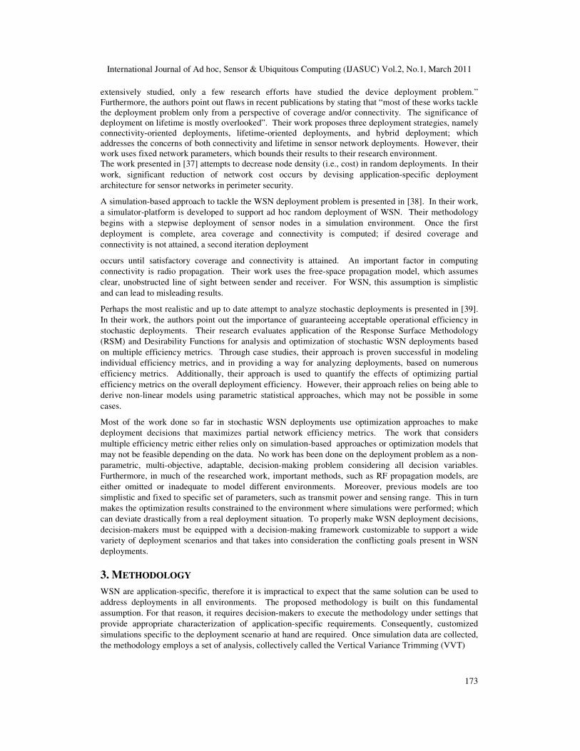
technique, to eliminate statistically redundant deployment alternatives. Therefore, VVT provides decreased number of deployment alternatives but equal characterization of the original deployment scenario. Finally, the reduced set of deployment alternatives are analyzed with AHP to rank deployment alternatives based on deployment goals. An overview of the methodology is presented in Figure 1.

Figure 1. Methodology Overview

4. SIMULATION FRAMEWORK

Simulation of WSN has been the topic of much debate in the research literature. In [40], the authors

point to statistics on the percentage of articles in top conferences that do not specify the simulator,

transmission distance, and number of simulation runs. In addition, they point out the use of inappropriate

radio propagation models. For this reason, sufficient explanation of the simulation environment becomes

necessary. Simulation of WSN deployments should, at a minimum, provide information about network

connectivity, coverage, cost, and lifetime. Therefore, simulation of radio frequency (RF) signal

propagation is essential. Simulation of RF signal propagation is challenging due to the distance-

dependent and time-variable energy loss (i.e., path loss) that the signal experience between transmitter

and receiver. Several theoretical models have been widely adopted in the WSN literature, including the

free-space, two-ray, and log-normal shadowing [41]. As specified in [42], the free-space and two-ray

models are not appropriate for WSN. In most practical applications, the received signal strength for the

same transmission distance will be different [43]. This variation due to location is referred as log-normal

shadowing and can be modeled using the log-normal shadowing model [44]. This capability of the log-

normal shadowing model can be used to model different terrain obstructions between transmitter and

receiver. For this reason, the log-normal shadowing model is used in the simulation environment.

By using the log normal shadowing model, transmission power can be estimated and related to overall network lifetime. Therefore, through RF propagation models, estimates of network lifetime can be easily obtained. To determine coverage, the simulation platform uses the Boolean sensing model, as described in [42]. Finally, cost is assumed directly proportional with the number of deployed nodes. For detailed description, verification, and validation of the simulation platform used in this research, readers can refer to [42].

5. VERTICAL VARIANCE TRIMMING

This section presents the Vertical Variance Trimming (VVT) technique devised for reducing the number

of alternatives available to decision-makers when analyzing the deployment problem. In the most trivial

case, VVT identifies all deployment alternatives as equal, which allow decision-makers to select any of

the available alternatives. In more complex scenarios, VVT helps reduce the number of deployment

strategies to simplify the decision-making process. VVT works by determining the effects of deployment

parameters on WSN network efficiency. WSN deployment decisions involve complex processes where


175

several varying factors are assumed to have significant effects on WSN efficiency. Typical assumptions include (1) higher network connectivity and area coverage is achieved by deploying higher number of nodes; (2) higher radio and sensing range result in higher connectivity and area coverage; and (3) high degree of terrain obstructions requires sensor nodes to use higher transmission power to achieve equal connectivity as in environments with low terrain obstructions. These are all valid assumptions, however the degree to which they are significant needs to be determined

before making deployment decisions. To determine significance, VVT uses the balanced and fixed-

effects single factor Analysis of Variance (ANOVA) and Least Significance Difference (LSD) methods

[45]. Once significance is determined, the critical metric value (CMV) is determined to determine the

minimum acceptable efficiency of the initial deployment. Because single factor ANOVA is an essential

part of VVT, an in-depth discussion of the ANOVA procedure is required.

5.1 Single Factor ANOVA ANOVA is a statistical procedure to test the equality of two or more population means. It works by analyzing the total variation of the data, specifically, the (1) variability within each treatment (i.e. factor level), and (2) variability between treatments. The variability found within treatments is attributed to random error while the variability found between treatments is attributed to the effects that the different treatments have in the response variable. If the variability caused by random error is similar to the variability caused by having different treatments, it is assumed that the observed differences in treatments means are caused by random error and not by using different treatments. Otherwise, the observed differences in treatment means are assumedly caused by using different treatments. Single Factor ANOVA relies on the following three main assumptions [45]: the errors are normally

distributed; the errors are independent; and the errors have constant variance.

The first assumption states that the difference between any observed value and its respective sample

mean (i.e., the errors) should be random, and that the error from one observed value should not influence

error in another observed value. The second assumption states that the data from each factor level should

come from a normal distribution. This assumption can be easily checked using a normal probability plot

or chi-square goodness of fit test. The third assumption states that the variances present in the data for

each factor level are equal.

The second and third assumption refers to the behavior of the variable being collected [46]. However,

the ANOVA in the WSN deployment problem uses a balanced with fixed effects model, which is robust

to the normality assumption and is only slightly affected by violations of homogeneity in variances [45,

47, and 48].

ANOVA uses the F statistical test to compare the differences between the estimated variance due to

random error and the estimated variance due to difference in treatments. The variance caused by random

error is obtained by calculating the Sum of Squares due to Error (SSE) divided by its number of degrees

of freedom. The variance caused by differences in treatments is obtained by calculating the Sum of

Squares due to Treatments (SST) divided by its number of degrees of freedom. The test statistic F is

computed using (1) [45].

(1)

where N is the total number of observations and a is the total number of treatments. Once the test

statistic F is calculated, the next step involves computing the critical value of F (FCRIT), which is the

maximum value required to accept the null hypothesis at the specified significance levelα . A

significance level of 1%, 5% and 10% are common in practice. The critical value of F is computed as

follow [45]:

(2) ( )αaNaCRIT FF−−

= ,1

( )( )aNSS

aSS

S

SF

E

T

−

−==

12

2

2

10


176

where ( )α2,1 vvF is a point in the F distribution table [45, 46] atα level of significance. Once the test

statistics F and FCRIT are computed, statistical differences among the treatments are suggested by

CRITFF > .

There are two main ways that single factor ANOVA can be used to obtain useful insight into the WSN

deployment dynamics. Table II displays identified use cases for single factor ANOVA.

Table 1. Single Factor ANOVA Use Cases

Case Number of

Nodes

Radio

Range

Sensor

Range Terrain Output

1 Variable Fixed Fixed Fixed Connectivity

2 Variable Fixed Fixed Fixed Coverage

In both cases, the effects of varying the number of deployed nodes on network connectivity and area

coverage are determined by using a fixed set of values for radio range, sensor range, and terrain. These

are representative of deployments where sensor nodes have fixed capabilities and terrain conditions are

known in advance. Once the experimental use cases have been defined, the following steps are

performed on each use case to determine the effects of the variable factor (i.e., columns 2 to 5) on the

response variable of interest (i.e., column 6).

5.1.1 A. Step 1 - Formulate the Null Hypothesis

This step involves selecting the factor of interest, determining the levels of the factor to analyze, and stating the NULL hypothesis. For example, the effects of varying the number of deployed nodes on overall WSN connectivity can be determined by selecting number of nodes as factor of interest, varying the levels between 50 to 300 meters (in increments of 10), and stating the null hypothesis as follows:

As seen, the null hypothesis assumes no mean differences (in connectivity) between the various levels of

number of nodes. The results of the ANOVA are used to justify rejection of the null hypothesis.

5.1.2 B. Step 2 - Compute Variance due to Random Error

The dispersion in data around the mean of a single factor level is assumedly caused by random error [45]. Variance caused by random error is estimated by computing and converting the Sum of Squares due to Error (SSE) into a variance estimate [45]. First, SSE is computed by iterating through each factor level, while adding each squared deviate, which is the distance from a particular observed value from its mean. SSE can be computed using (3) [45].

(3)

Once SSE is computed, it is converted to a variance estimate by dividing it by its number of degrees of

freedom, N-a, where N represents the total number of observations and a represents the total number of

treatments. The variance caused by random error is estimated using (4) [45].

(4)

300...7060500 : xxxxxH ====

aN

SSS E

−=

2

1

( )2

∑∑ −=

g

l

n

j

ljlE xxSS


177

5.1.3 C. Step 3 - Compute Variance due to Treatment Variance due to different treatments is estimated by computing and converting the Sum of Squares due to Treatment (SST) into a variance estimate. SST is computed by iterating through each factor level, while adding the squared difference of each level’s mean and the overall mean. SST is computed using (5) [45].

(5)

SST is converted to a variance estimate by dividing it by its number of degrees of freedom, a-1, where a is

the total number of levels. The variance caused by using different levels is computed using (6) [45].

(6)

5.1.4 D. Step 4 - Compute the Sum of Squares Total This step should be done to make sure that your previous calculation of SSE and SST are correct. Since SSTOTAL = SSE + SST then the sum of SSE and SST should equal the calculated value of SSTOTAL. SSTOTAL is computed using (7) [45].

(7)

5.1.5 E. Step 5 - Calculate the test statistic F The test statistic F calculates the ratio between the variability caused by random error and the variability caused by having different alternatives, as seen in (2).

5.1.6 F. Step 6 - Calculate the critical value of F and make decision The critical value of F (FCRIT) is the maximum value required to accept the null hypothesis at a specified significance level α. This means that the null hypothesis is rejected when F0> FCRIT. FCRIT is obtained using (2).

5.2 Least Significance Difference (LSD) Method The LSD test is used on pair of deployment strategies to determine their statistical equality. Two deployment strategies are different if the difference in their mean response (i.e., connectivity, coverage) is greater than the least significant difference; which for balanced experimental data, is obtained as specified in [45]. Otherwise, they are considered statistically similar. When this occurs, decision-makers can eliminate the redundant strategy that results in increased cost. Once all the deployment strategies have been analyzed using LSD, the CMV is used to further reduce the deployment alternative set to match specific application requirements.

5.3 Critical Metric Value (CMV) Once redundant deployment strategies have been removed, the CMV is selected to identify the minimum value for the decision metric that decision-makers are willing to accept for initial deployment. Deployment strategies resulting in values higher than the CMV are considered for initial deployment.

( )∑=

−=a

i

iT xxnSS1

2

1

2

2−

=a

SSS T

( )2

1 1

∑∑= =

−=a

i

n

j

ijTOTAL xxSS


178

Deployment strategies resulting in values below the CMV are considered for re-deployment to fill gaps and correct initial deployment. With this final step, VVT reduces the number of deployment alternatives significantly, which simplifies the application of the AHP.

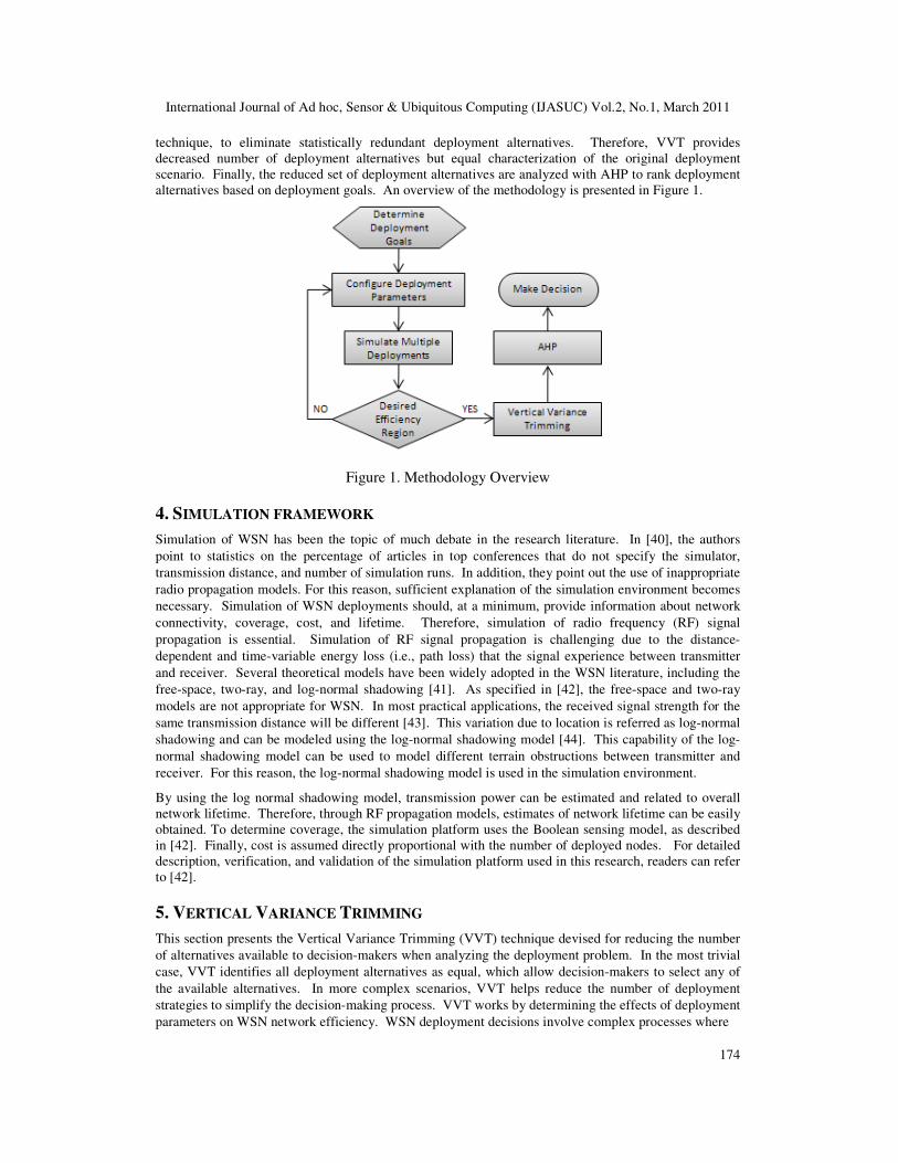
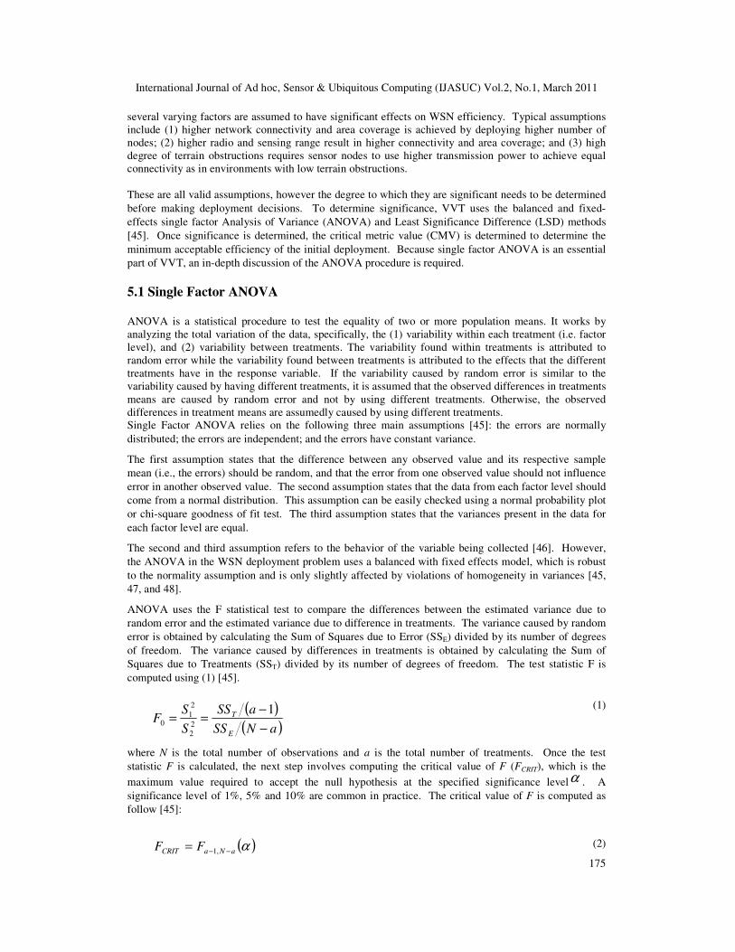
5.4 Case Study 1 - Vertical Variance Trimming This case study provides analysis of random WSN deployments using VVT. It assumes a rectangular deployment area measuring 500 m x 500 m, 50 to 100 nodes available for deployment with onboard radio capable of transmitting between 50 to 100 meters and sensors capable of covering between 30 to 60

meters. Simulation results for connectivity and coverage are presented in Figures 1 and 2, respectively.

Figure 2. Connectivity Results

Figure 3. Coverage Results

Deployment strategies are composed of specific number of nodes, radio range, and sensor range. Since

there are 50, 60, …, n alternatives for number of nodes; 40, 45, …, r alternatives for radio range; and 30,

35, …, s alternatives for sensor range, the initial deployment decision consists of n x r x s = 546

alternatives. The goal of VVT is to reduce the number of deployment alternatives while maintaining the

same significance of the original deployment scenario. VVT is applied to each network metric (e.g.,

connectivity, coverage) as follow.

5.4.1 A. Step 1 – Determining Significance Using Figures 1 and 2, for each column, ANOVA is performed (vertically) to trim out deployment strategies that result in statistically similar outputs. If statistical differences are found, the LSD is used to identify the redundant strategies. Similar strategies are grouped together using the following rules: (a) strategies that belong to two separate groups will join the group with the highest number of strategies; and (b) strategies that belong to two separate groups of same number of strategies will join either group, based on decision-makers' preference.


179

5.4.2 B. Step 2 – Selection of Critical Metric Value (CMV) Critical Metric Value (CMV) is the minimum value for the decision metric that decision-makers are willing to accept for initial deployment. Deployment strategies resulting in values higher than the CMV are considered for initial deployment. Deployment strategies resulting in values below the CMV are considered for re-deployment to fill gaps and correct initial deployment. The initial deployment alternatives in terms of connectivity include n x r = 78 alternatives. Using

Vertical Trimming, the number of deployment alternatives is reduced to 51, which reduces the overall

number of deployment strategies from 546 to 357, resulting in 35% reduction of decision alternatives.

The deployment alternatives for connectivity are summarized in Table II.

Table 2. Results of Vertical Trimming on Connectivity

Nodes Radio Ranges

50 40, 45, 50, 55, 60, 65, 70, 75, 80, 85, 90, 95, 100

60 50, 55, 60, 65, 70, 75, 85, 90, 95, 100

70 45, 55, 60, 65, 70, 75, 80, 85, 90, 95

80 40, 50, 55, 70, 75, 85, 90 90 40, 45, 55, 60 65, 70, 75, 80

100 50, 55, 65

Using CMV = 90%, the alternatives for initial deployment are reduced to 5, which results in 94%

reduction in deployment alternatives from the initial set. The deployment alternatives at CMV = 90% for

connectivity are displayed in Table III.

Table 3 Deployment Alternatives for Conn. at CMV = 90%

Nodes Radio

Ranges

50 100

60 95 60 100

70 95 80 90

For coverage, the initial deployment alternatives include n x s = 42 alternatives. Using Vertical Trimming, the number of alternatives is reduced to 39, which results in 7% reduction of decision alternatives. This means that the original set of deployment alternatives are significantly different from one another. Using CMV = 40%, the results are obtained and combined with the connectivity results to obtain the final list of deployment alternatives.

6. DECISION-MAKING WITH AHP

The Analytical Hierarchy Process (AHP) can be used to determine the best deployment strategy for a

given WSN application. The AHP is a multi-attribute decision-making method used to facilitate

decisions that involve multiple competing criteria [49]. AHP is extremely popular and has been applied

by decision-makers in countless areas including highway engineering, economics, energy, management,

climate control, computer science, engineering, agriculture, and the military [50, 51].

AHP provides a powerful tool that can be used to make decisions in situations involving multiple

objectives [50]. Specifically, it can transform the WSN deployment problem into a structured hierarchy

where each decision-making unit is quantified and related to overall goals for evaluating alternative

solutions [51]. The WSN deployment problem encounters the following conflicting goals:


180

• Minimize deployment cost

• Maximize network connectivity

• Maximize network coverage

• Maximize network lifetime

These objectives are representative of typical WSN deployments. However, specific application

requirements may give rise to objectives containing variations of these general objectives. For example,

multi-segment WSN require high connectivity and high coverage for the Sensing & Relaying Segment

(SRS), but high connectivity and low coverage for the Relaying Segment (RS) [37]. Other examples

include WSN that use small autonomous vehicles after deployment to fill existing connectivity gaps in

the network. In these applications, high area coverage with extended network lifetime is desired over

high connectivity. These are a few examples that demonstrate the application-specific and complex

nature of the deployment problem and serve as justification for the use of quantitative methods such as

AHP for decision-making.

The first step in the decision-making process involves the creation of the AHP hierarchy. This requires

the decision-maker to have complete knowledge of resources available for deployment. Once the AHP

hierarchy is complete, prioritized deployment strategies are created using simulation data, a pairwise

comparison scale, and the AHP pairwise comparison matrices.

6.1 AHP Hierarchy Creation

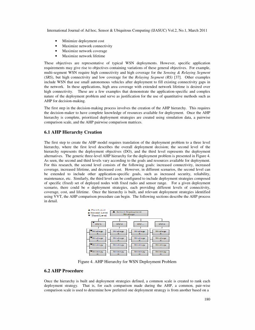
The first step to create the AHP model requires translation of the deployment problem to a three level hierarchy, where the first level describes the overall deployment decision; the second level of the hierarchy represents the deployment objectives (DO), and the third level represents the deployment alternatives. The generic three-level AHP hierarchy for the deployment problem is presented in Figure 4. As seen, the second and third levels vary according to the goals and resources available for deployment. For this research, the second level consists of the following goals: increased connectivity, increased coverage, increased lifetime, and decreased cost. However, in different scenarios, the second level can be extended to include other application-specific goals, such as increased security, reliability, maintenance, etc. Similarly, the third level can be configured to include deployment strategies composed of specific (fixed) set of deployed nodes with fixed radio and sensor range. For a given deployment scenario, there could be n deployment strategies, each providing different levels of connectivity, coverage, cost, and lifetime. Once the hierarchy is built, and relevant deployment strategies identified using VVT, the AHP comparison procedure can begin. The following sections describe the AHP process in detail.

Figure 4. AHP Hierarchy for WSN Deployment Problem

6.2 AHP Procedure

Once the hierarchy is built and deployment strategies defined, a common scale is created to rank each deployment strategy. That is, for each comparison made during the AHP, a common, pair-wise comparison scale is used to determine how preferred one deployment strategy is from another based on a


181

specific deployment objective. This allows standardization in all comparisons made during the AHP process. Table IV presents the pairwise comparison scale created for the deployment problem.

Table 4. Pairwise Comparison Scale

Scale (w) Description

1 Equally Preferred 2 Equally to Moderately Preferred

3 Moderately Preferred

4 Moderately to Strongly Preferred 5 Strongly Preferred

The pairwise comparison scale is used by decision-makers to establish preferences between different

alternatives. The next step is to create n pairwise comparison matrices [50] to evaluate and determine

relative importance between alternatives present in the WSN deployment scenario. There are two types

of pairwise comparison matrices in AHP, the Alternative-Alternative matrix, and the Objective-Objective

matrix.

6.3 Alternative-Alternative Pair-wise Comparison Matrix

The Alternative-Alternative pairwise comparison matrices are n x n matrices where each location aij

represents how much more important the deployment strategy at row i is than the strategy at column j, in

terms of a pre-defined deployment goal (e.g., connectivity, coverage, cost). The format of these matrices

for the deployment problem is presented in (8), where Az is the pairwise comparison matrix for objective

z (i.e., z ∈{connectivity, coverage, lifetime, cost}) and Sx represents deployment strategy x.

(8)

Once the pairwise comparison matrices are defined, weight vectors are computed from each pairwise

comparison matrix. Weigh vectors contain the relative importance of each deployment strategy in the

pairwise comparison matrix. That is, assuming weight vector w = [w1 w2 ... wn], , the value of wi

represents the relative importance of deployment strategy i of the associated pairwise comparison matrix

based on objective z. The weight vectors are used to make the final decision. To compute the weight

vectors, the pairwise comparison matrix needs to be normalized as shown in (9),

(9)

where aij represents the ath element at row i and column j of the respective standard alternative/alternative

=

nnnn

n

n

n

n

z

wwwwww

wwwwww

wwwwww

S

S

S

SSS

A

L

OMM

L

L

M

L

21

22212

12111

2

1

21

=

∑∑

∑∑

==

==

n

i

in

nn

n

i

i

n

n

i

in

n

n

i

i

norm

a

a

a

a

a

a

a

a

A

11

1

1

1

1

1

1

11

L

MOM

L


182

comparison matrix. Once in normalized form, the weight vector associated with Anorm can be computed using (10).

(10)

6.4 Objective-Objective Pairwise Comparison Matrix

The Objective-Objective pairwise comparison matrix is a n x n matrix where each location aij represents

how much more important the deployment objective (e.g., connectivity, cost, etc.) at row i is than the

deployment objective at column j. Its purpose is to provide a ranking that captures decision-makers

preferences between deployment goals for WSN deployments. The Objective-Objective matrix format

for the WSN deployment problem is presented in (11), where wi is the weight given to objective i. Once

the Objective-Objective matrix is created, it is normalized and the weight vector is computed using the

same procedure as in the Alternative-Alternative matrices.

=

nnnn

n

n

wwwwww

wwwwww

wwwwww

Life

Cos

Cov

Con

LifeCosCovCon

A

L

MOMM

L

L

21

22212

12111

(11)

6.5 AHP Evaluation Results

Once all weight vectors in the decision problem have been computed, AHP uses these weights to

determine the best alternative. For example, assuming a deployment problem with x number of

objectives and y number of deployment strategies, the AHP provides y+1 weight vectors; one (wA)

associated with the Objective-Objective pair-wise comparison matrix, and the rest wi associated with

each Alternative-Alternative matrix i, as illustrated in Figure 5.

−

nnnnn

T

A

T

y

TTT

w

w

w

w

w

w

w

w

w

w

w

w

w

w

w

wwwww

MMMMM

L

2

1

2

1

2

1

2

1

2

1

121

Figure 5. Weight Vectors for the Deployment Problem

To compute the relative preference for deployment strategy i, we let Wik represent the ith row of the kth

(transposed) weight vector, WAk represent the kth element of the WA vector, and Si as the overall score for

deployment strategy i,

Si = ( )k

y

k

ik WAW∑=1

(12)

====

∑∑∑===

n

a

wn

a

wn

a

ww

n

j

nj

n

n

j

j

n

j

j

11

2

2

1

1

1 L


183

where k represents the k

th element of vectors W and WA. Once overall scores are computed for all deployment strategies, the highest score is identified as the best alternative, followed by the second highest score, and so on. This prioritized list helps decision-makers in selecting the deployment strategies even if the best strategy cannot be selected.

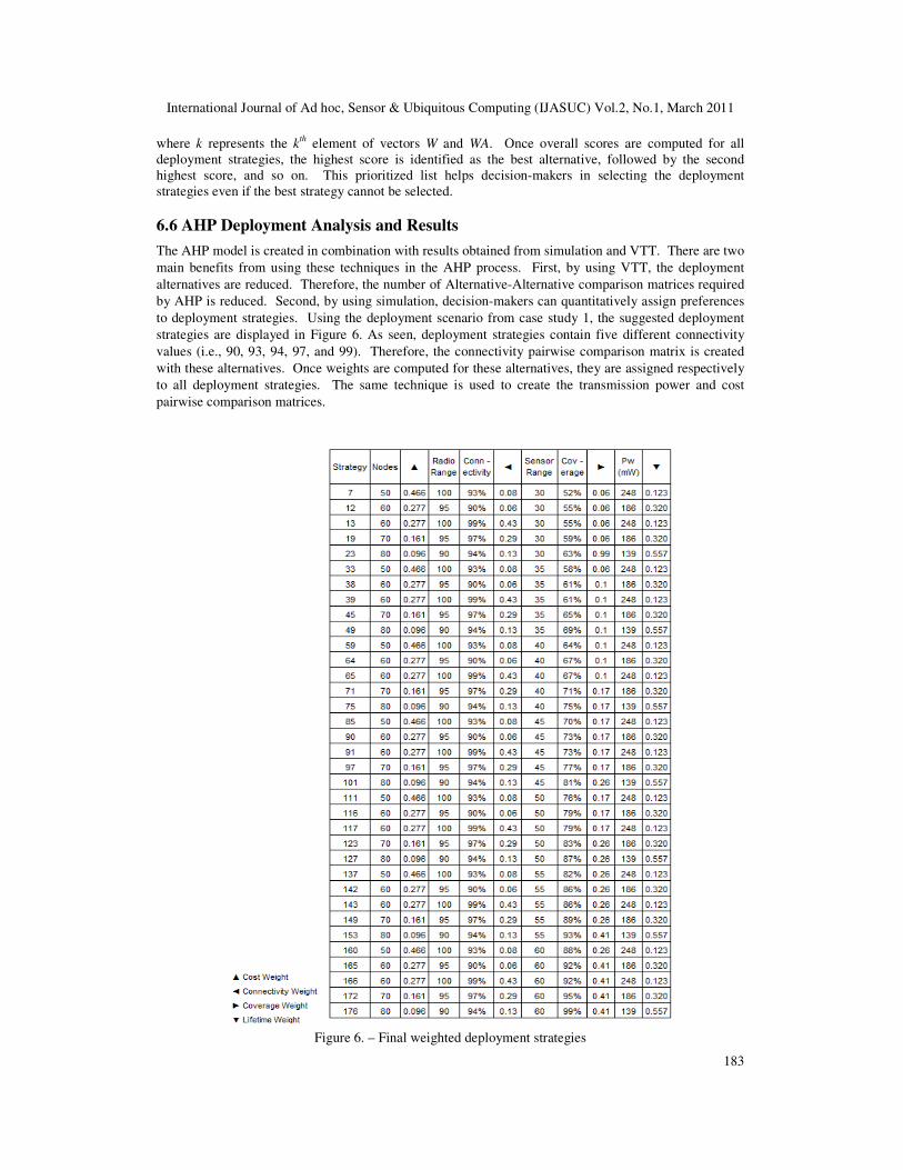
6.6 AHP Deployment Analysis and Results

The AHP model is created in combination with results obtained from simulation and VTT. There are two

main benefits from using these techniques in the AHP process. First, by using VTT, the deployment

alternatives are reduced. Therefore, the number of Alternative-Alternative comparison matrices required

by AHP is reduced. Second, by using simulation, decision-makers can quantitatively assign preferences

to deployment strategies. Using the deployment scenario from case study 1, the suggested deployment

strategies are displayed in Figure 6. As seen, deployment strategies contain five different connectivity

values (i.e., 90, 93, 94, 97, and 99). Therefore, the connectivity pairwise comparison matrix is created

with these alternatives. Once weights are computed for these alternatives, they are assigned respectively

to all deployment strategies. The same technique is used to create the transmission power and cost

pairwise comparison matrices.

Figure 6. – Final weighted deployment strategies


184

Coverage values range from the 50th to the 90th percentile. To simplify the AHP pairwise comparison

matrix for coverage, the groups in Table V are created. Using the pairwise comparison scale from Table

IV and the deployment strategy data from Figure 6, AHP computes pairwise comparison matrices,

normalized matrices, and weight vectors. The results for connectivity, coverage, cost and lifetime are

presented in Tables V to IX., respectively.

Table 5. Coverage groups For pairwise comparisons

Group Values 50 52%, 55%, 58%, 59%

60 61%, 63%, 64%, 65%, 67%, 69%

70 70%, 71%, 73%, 75%, 76%, 77%, 79%

80 81%, 82%, 83%, 86%, 87%, 88%, 89%

90 92%, 93%, 95%, 99%

Table 6. Connectivity Pairwise Comparison Matrix, Normalized Matrix and Weight Vector

Connectivity - Pairwise Comparison

% 99 97 94 93 90

99 1 2 4 5 5

97 0.50 1 3 4 5

94 0.25 0.33 1 2 3

93 0.20 0.25 0.50 1 2

90 0.20 0.20 0.33 0.50 1

Total 2.15 3.78 8.83 12.50 16.00

Connectivity - Normalized Matrix

% 99 97 94 93 90

99 0.465 0.529 0.453 0.400 0.313

97 0.233 0.265 0.340 0.320 0.313

94 0.116 0.087 0.113 0.160 0.188

93 0.093 0.066 0.057 0.080 0.125

90 0.093 0.053 0.037 0.040 0.063

Connectivity - Weight Vector

99 97 94 93 90

w 0.432 0.294 0.133 0.084 0.057

Table 7. Coverage Pairwise Comparison Matrix, Normalized Matrix and Weight Vector

Coverage - Pairwise Comparison

% 90 80 70 60 50

90 1 2 3 4 5

80 0.50 1 2 3 4

70 0.33 0.50 1 2 4

60 0.25 0.33 0.50 1 2

50 0.20 0.25 0.25 0.50 1

Total 2.28 4.08 6.75 10.50 16.00

Coverage - Normalized Matrix

% 90 80 70 60 50

90 0.438 0.490 0.444 0.381 0.313

80 0.219 0.245 0.296 0.286 0.250

70 0.146 0.122 0.148 0.190 0.250

60 0.109 0.082 0.074 0.095 0.125

50 0.088 0.061 0.037 0.048 0.063


185

Coverage - Weight Vector

90 80 70 60 50

w 0.413 0.259 0.171 0.097 0.059

Figure 6 presents full characterization of deployment strategies. That is, statistically redundant strategies

have been removed using VVT and each deployment strategy has been assigned a weight for each

deployment goal based on results obtained from AHP. At this point, this information can now be

combined with the Objective-Objective comparison matrix to provide decision-makers with prioritized

alternatives based on specific WSN deployment mission.

Table 8. Cost Pairwise Comparison Matrix, Normalized Matrix and Weight Vector

Cost - Pairwise Comparison

Nodes 50 60 70 80

50 1 2 3 4

60 0.50 1 2 3

70 0.33 0.50 1 2

80 0.25 0.33 0.50 1

Total 2.08 3.83 6.50 10.00

Cost - Normalized Matrix

Nodes 50 60 70 80

50 0.480 0.522 0.462 0.400

60 0.240 0.261 0.308 0.300

70 0.160 0.130 0.154 0.200

80 0.120 0.087 0.077 0.100

Cost - Weight Vector

Nodes 90 80 70 60

w 0.466 0.277 0.161 0.096

Table 9. Lifetime Pairwise Comparison Matrix, Normalized Matrix and Weight Vector

Lifetime - Pairwise Comparison

mW 139 186 248

139 1 2 4

186 0.50 1 3

248 0.25 0.33 1

Total 1.75 3.33 8.00

Lifetime - Normalized Matrix

mW 139 186 248

139 0.571 0.600 0.500

186 0.286 0.300 0.375

248 0.143 0.100 0.125

Lifetime - Weight Vector

mW 139 186 248

w 0.557 0.320 0.123

6.7 Case Study 2 – Lifetime, Connectivity, Cost, Coverage

This section presents the results of AHP (i.e., prioritized list of deployment strategies) when lifetime is of

most importance, followed by connectivity, cost, and coverage. As seen in Figure 6, Lifetime is equally

to moderately preferred to connectivity, moderately preferred to cost, and moderately to strongly

preferred to coverage. Also, connectivity is equally to moderately preferred to cost, and moderately

preferred to coverage. Finally, cost is moderately preferred to coverage. Using (12), final scores are


186

computed and a prioritized list of deployment strategies based on the Objective-Objective comparison matrix is created, as seen in Figure 6. For practical considerations, only the top 19 deployment alternatives are shown in this and all subsequent case studies. As seen, strategy #23, which consists of deploying 80 nodes with radio range of 90 m, and sensor range of 30 m, provides the best relative deployment alternative, followed by strategy #153, #176, #101, and so forth.

Figure 7. Objective-Objective Matrix and Prioritized Deployments

6.8 Case Study 3 – Connectivity, Cost, Coverage, Lifetime

This section presents the results of AHP when connectivity is of most importance, followed by cost,

coverage, and lifetime. As seen in Figure 7, simply by changing the Objective-Objective evaluation

scores, the AHP produces a new prioritized list reflecting the new deployment goals. Using (12), final

scores are computed and a new prioritized list of deployment strategies based on the Objective-Objective

comparison matrix is created, as seen in Figure 7. In this scenario, strategy #166, which consists of

deploying 60 nodes with radio range of 100 m, and sensor range of 60 m, provides the best relative

deployment alternative, followed by strategy #143, #23, #91, and so forth. By changing the deployment

goals, strategies #153, #176, and #101 are no longer in the top 4 strategies, which differs from the results

obtained in the previous case study.

6.9 Case Study 4 –Cost, Coverage, Connectivity, Lifetime

Finally, this section presents the results of AHP when cost is of most importance, followed by coverage,

connectivity, and lifetime. As seen in Figure 8, strategy #23, provides the best relative deployment

alternative, followed by strategy #166, #137, #160, and so forth. An interesting pattern is seen in case

studies 3, 4, and 5. That is, even though deployment goals are varying, certain deployment strategies

continue to show up as top deployment strategies, for example, strategies #23 and #166. This suggests a

different avenue for deployment decision making, where all possible combinations of deployments' goal

rankings are made, and deployment strategies are selected based on the highest recurring strategy among

all evaluations. For example, in these case studies, strategy #23 appears among the top 4 strategies in all

scenarios; while strategy #166 appears among the top 4 strategies in 2 out of 3 cases. This could lead to

the selection of strategy #23 and #166 as the best deployment strategies, in that order.


187

Figure 8. Cost matrix, normalized matrix, and weight vector

Figure 9. Cost, Coverage, Connectivity, Lifetime

7. CONCLUSION & FUTURE WORK

The research presented in this paper develops a systematic approach for planning WSN stochastic

deployments based on multiple deployment goals. Specifically, it presented a methodology that uses

simulation, statistical analysis, and AHP to analyze and optimize stochastic deployments.

There are several important contributions from this research. The main contribution is the capability for

analyzing stochastic deployments based on multiple goals without requiring predictive mathematical

models. The advantage of analyzing the deployment problem without predictive mathematical models is

that analysis is always feasible. By not requiring derivation of mathematical models, analysis can be

performed straight from simulation data. However, in most cases, the vast amounts of data provided by


188

the simulator can significantly increase the complexity of decision-making. For this reason, techniques such as VVT are desired. The results presented in this research show how the VVT technique works well for statistical analysis of

simulated deployment data. By applying VVT, results showed as much as 35% minimization of

deployment strategies. By combining the resulting solutions with the CMV threshold value, maximum

reduction of deployment strategies are achieved. These results significantly contributed to the success of

the AHP decision-making technique.

The AHP approach is straightforward and worked well for the deployment problem. However, as the

number of comparisons increase, so does the complexity of the AHP model. For this reason, it is

suggested the automation (via software) of the AHP technique. In addition, the AHP lacks the capability

of interpolating, which requires simulation of every deployment strategy. This problem is also easily

resolved through software automation, where all deployments strategies can be simulated and analyzed

right away with AHP using customized software. Considering the potentially high complexity, and lack

of interpolation capabilities, AHP still proves to be a feasible and strong technique for managing and

planning stochastic WSN deployments.

Although the presented approach serves well to provide decision-making support for stochastic WSN

deployments, several areas can be improved to increase the quality of predictions and enhance the overall

quality of proposed solutions. Individual improvements and future areas of research are provided as

follow.

7.1 Terrain Classification

Terrain characteristics can significantly alter the quality of the results provided by the deployment methodology. Therefore, terrain analysis and classification of specific deployment areas should be incorporated. Since deployment of large-scale WSN can take place in vast areas containing various terrain characteristics, a suggested approach involves segregating the deployment area in different cells based on different terrain characteristics. By dividing the deployment area in different cells with equal terrain characteristics, appropriate RF propagation models can be used in each terrain cell to account for increased resources required to achieve desired network efficiency in that section of the deployment area. With this information, a sum of the resources used in all cells can be used to estimate overall resource usage for the deployment to be effective. In practical scenarios, once deployed, the nodes in each cell can be configured via software to adjust their parameters (e.g., radio range) to match the planned network efficiency.

Terrain classification can be achieved using artificial neural networks. Recent work presented in [52] uses neural networks to classify terrain into 5 categories, including flat plane, rugged terrain, grassy terrain, incline plane and unclassified. Their results showed 100% correctness for classification of flat planes, rugged, and incline terrains, and 80% correctness for grassy terrains. A similar neural networks approach can be used to analyze digital imagery of deployment areas, classify the terrain, and improve the overall simulation process.

7.2 Detection of Random Target Events

This research presents the coverage metric as the number of points sensed by the WSN in the deployment area to the total number of points in the deployment area. Although this metric provides the most comprehensive estimate of area coverage, it may not be the most practical for some WSN applications. An alternate approach for computing coverage is to determine the probability of a random event being covered. This new metric can be included in the data collection and analysis process to represent deployment strategies that result in higher coverage efficiency with reduced number of deployed nodes (i.e., cost).


189

7.3 Decision Support System Software All analysis, models, and techniques should be combined with software to provide a fully functional decision support system (DSS) software for stochastic deployment of WSN. The DSS can serve as platform to provide decision-makers with proper analysis based on customized deployment scenarios that include a variety of terrains areas and other conditions affecting network efficiency. Future work should investigate soft-computing techniques that are tolerant to imprecision, uncertainty, partial truth, and approximation [53]. Soft-computing techniques include fuzzy system, neural networks, evolutionary computation, machine learning, and probabilistic reasoning. In some cases, these techniques, or their combination, can be use to solve problems more effectively [53]. If appropriate, these techniques can be incorporated into the decision-making process when evaluating stochastic deployments of WSN.

REFERENCES

[1] Karl, H., Willig, A., Protocols and Architectures for Wireless Sensor Networks, Wiley, 1st Edition, 2007. [2] Akyildiz, I.F., Su, W., Sankarasubramaniam, Y., Cayirci, E., “Wireless Sensor Networks: A Survey,"

Computer Networks 38 (4) (2002) 393-422. [3] Younis, M., Akkaya, K., “Strategies and Techniques for Node Placement in Wireless Sensor Networks: A

Survey,” Ad Hoc Networks, 6 (2008) 621-655. [4] Dhillon, S.S., Chakrabarty, K., “Sensor Placement for Effective Coverage and Surveillance in Distributed

Sensor Networks,” Proceedings of IEEE Wireless Communications and Networking Conference, New Orleans, LA, March, 2003.

[5] Efrat, A., Har-Peled, S., Mitchell, J.S.B., “Approximation Algorithm for Two Optimal Location Problems in Sensor Networks,” Proceedings of the 3rd International Conference on Broadband Communications, Networks

and Systems, Boston, Massachusetts, October, 2005. [6] Cheng, X., Du, DZ, Wang, L., Xu, B., “Relay Sensor Placement in Wireless Sensor Networks,” IEEE

Transactions on Computers, 56(1):134-138, 2007. [7] Grandham, S.R., Dawande, M., Prakash, R., Venkatesan, S., “Energy Efficient Schemes for Wireless Sensor

Networks with Multiple Mobile Base Stations,” Proceedings of the IEEE Globecom, San Francisco, CA, December, 2003.

[8] Pan, J., Cai, L., Hou, Y.T., Shi, Y., Shen, S.X., “Optimal Base-Station Locations in Two-Tiered Wireless Sensor Networks,” IEEE Transactions on Mobile Computing, 4(5):458-473, 2005.

[9] Pan, J., Hou, Y.T., Cai, L., Shi, Y., Shen, S.X., “Locating Base-Stations for Video Sensor Networks,” Proceedings of the IEEE Vehicular Technology Conference, Orlando, FL, October, 2003.

[10] Hill, J., Culler, D., MICA: A Wireless Platform for Deeply Embedded Networks, IEEE Micro, 22(6): 12-14, 2002

[11] Rabaey, J., Ammer, J., da Silva, J.L., Patel, D., Pico-Radio: Ad-hoc Wireless Networking of Ubiquitous Low Energy Sensor/Montior Nodes, Proceedings of the IEEE Computer Society AnnualWorkshop on VLSI, pp. 9-12, Orlando, FL, April 2000

[12] BTnodes - A Distributed Environment for Prototyping Ad Hoc Networks, http://www.btnode.ethz.ch, Retrieved on August 16, 2008

[13] ScatterWeb, http://www.scatterweb.de/content/products/node_en.html, Retrieved on August 16, 2008 [14] EYES, http://www.eyes.eu.org/sensnet.htm, Retrieved on August 16, 2008 [15] µAMPS, http://mtlweb.mit.edu/researchgroups/icsystems/uamps/, Retrieved on August 16, 2008 [16] Pottie, G.J., Kaiser, W.J., Wireless Integrated Network Sensors, Communications of the ACM 43 (5) (2000)

551-558 [17] Kostanic, I., Subramanian, C.S., Pinelli, J.-P., Buist, L., Velazquez, A., and Wittfeldt, A., “Monitoring of

Hurricane Wind Pressures and Wind Speeds on a Residential Home Roof with Wireless Instrumentation,” in proceedings of Structural Engineering Congress, Vancouver, Canada, April 24-26, 2008.

[18] Brain, M., How Motes Work, http://computer.howstuffworks.com/mote.htm/printable, Retrieved on August 16, 2008

[19] Bonnet, P., Seshadri, G.P., Querying the Physical World, IEEE Personal Communications (October 2000), 10-15.

[20] ALERT, http://www.alertsystems.org, Retrieved on August 16, 2008 [21] Estrin, D., Culler, D., Pister, K., Sukhatme, G., Connecting the physical world with pervasive networks. IEEE

Pervasing Computing, 2002 [22] Chandrakasan, A., Sheng, S., Brodersen, R., Low Power CMOS Digital Design, IEEE Journal of Solid-State

Circuits, 27(4): 473-484, 1992


190

[23] Heinzelman, W., Chandrakasan, A., Balakrishnan, H., Energy Efficient Communication Protocol for Wireless

Microsensro Networks, In Proceedings of 33rd Hawaii International Conference Sys. Sci., 2002 [24] Heinzelman, W., Kulik, J., Balakrishnan, H., Adaptive Protocols for Information Dissemination in Wireless

Sensor Networks, In Proceedings of 5th ACM/IEEE Mobicom, Seattle, WA, 1999 [25] Intanagonwiwat, C., Govindan, R., Estrin, D., Directed Diffusion: A Scalable and Robust Communication

Paradigm for Sensor Networks, ACM Mobicom 2000, Boston, MA, 2000 [26] Lindsey, S., Raghavendra, C., PEGASIS: Power Efficient Gathering in Sensor Information Systems, IEEE

Aerospace Conference, 2002 [27] Brooks, A., Makarenko, A., Kaupp, T., Williams, S., Durrant-Whyte, H., Implementation of an Indoor Active

Sensor Network, Proceedings of the 9th International Symposium on Experimental Robotics, Singapore, June, 2004

[28] Petrushin, V.A., Wei, G., Shakil, O., Roqueiro, D., Gershman, V., Multiple-Sensor Indoor Surveillance System, Proceedings of the 3rd Canadian Conference on Computer and Robot Vision, Quebec, June, 2006

[29] Berry, J., Fleischer, L., Hart, W.E., Phillips, C.A., “Sensor Placement in Municipal Water Networks”, Proceedings of the World Water and Environmental Resources Conference, Philadelphia, Pennsylvania, June, 2003

[30] Santi, P., Topology Control in Wireless Ad Hoc and Sensor Networks, ACM Computing Surveys, 37(2):164-194, 2005

[31] Chong, C.Y., Kumar, S.P., Sensor Networks: Evolution, Opportunities, and Challenges, Proceedings of the IEEE, 2003

[32] Clouqueur, T., Phipatanasuphorn, P.R., Saluja K.K., Sensor Deployment Strategy for Target Detection, Proceedings of 1st ACM International Workshop on Wireless Sensor Networks and Applications (WSNA ’02), 2002.

[33] Akkaya, K., Younis, M., COLA: A Coverage and Latency Aware Actor Placement for Wireless Sensor and Actor Networks, Proceedings of IEEE Vehicular Technology Conference, Montreal, Canada, September, 2006

[34] Ishizuka, M., Aida, M., Performance Study on Node Placement in Sensor Networks, Proceedings of the 24th International Conference on Distributed Computing Systems Workshops –W7:EC (Icdesw’04) –Volume 7, 2004

[35] Toumpis, S., Tassiulas, L., “Packetostatics: Deployment of Massively Dense Sensor Networks as an Electrostatic Problem,” Proceedings of the 24th IEEE Conference on Computer Communications and Networking, Miami, FL, March, 2005.

[36] Toumpis, S., Gupta, G.A., “Optimal Placement of Nodes in Large Scale Sensor Networks under a General Physical Layer Model,” Proceedings of the 2nd IEEE Conference on Sensor and Ad Hoc Communications and Networks, Santa Clara, CA, September, 2005.

[37] Otero, C.E., Kostanic, I., Otero, L.D, A Multi-hop, Multi-segment Architecture for Perimeter Security over Extended Geographical Regions using Wireless Sensor Networks, Proceedings of the 2008 IEEE Wireless Hive Network Conference, pp. 1-5, Aug. 2008.

[38] Bai, Y., Li, J., Han, Q., Chen, Y., Qian, D., Research on Planning and Deployment Platform for Wireless Sensor Networks, Advances in Grid and Pervasive Computing, LNCS 4459:199–210, 2007.

[39] Otero, C.E., Shaw, W.H., Kostanic, I., Otero, L.D., "Multi-Response Optimization of Stochastic WSN Deployments using Response Surface Methodology and Desirability Functions," IEEE Systems Journal, Vol 4, No. 1, pp. 39 - 48, 2010.

[40] Stojmenovic, I., “Simulations in Wireless Sensor and Ad Hoc Networks: Matching and Advancing Models, Metrics, and Solutions,” IEEE Communications Magazine, Vol. 46, No. 12, pp. 102-107, December, 2008.

[41] Fall, K., Varadhan, K., The ns Manual, http://www.isi.edu/nsman/ns/doc/ns_doc.pdf, July, 2008. [42] Otero, C.E., Kostanic, I., Otero, L.D., "Development of a Simulator for Stochastic Deployment of Wireless

Sensor Networks,” Journal of Networks, Vol. 4, No. 8, pp. 754-762, Oct. 2009. [43] Pahlavan, K., Krishnamurthy, P., Principles of Wireless Networks, Prentice Hall, 2002. [44] Rappaport, T.S., Wireless Communications: Principles and Practice, Prentice Hall, 1996. [45] Montgomery, D., Design and Analysis of Experiments, Wiley, 5th Edition, 2001 [46] Pelosi, M.K., Sandifer, T.M., Elementary Statistics: From Discovery to Decision, Wiley, 2003 [47] Trivedi, K.S., Probability & Statistics with Reliability Queuing and Computer Science Applications, Prentice-

Hall, 1982 [48] Harrell, C., Ghosh, B.K., Bowden, R.O., Simulation Using ProModel, McGraw Hill, 2004 [49] de Steiguer, J.E., Duberstein, J., Lopes, V., The Analytic Hierarchy Process as a Means for Integrated

Watershed Management, http://www.tucson.ars.ag.gov/icrw/Proceedings/Steiguer.pdf, Retrieved on August 9, 2008

[50] Winston, W.L., Operations Research: Applications and Algorithms, Duxbury, 4th Edition, 2003 [51] AHP, http://en.wikipedia.org/wiki/Analytic_Hierarchy_Process, Retrieved on August 17, 2008. [52] Jitpakdee, R., Maneewarn, T., Neural Networks Terrain Classification using Inertial Measurement Unit for an

Autonomous Vehicle, SICE Annual Conference 2008, Japan, 2008 [53] A Definition of Soft-Computing – adapted from L.A. Zadeh, http://www.soft-computing.de/def.html, Retrieved

on December, 2008

Documents

ANALYSIS OF WIRELESS SENSOR NETWORKS ...aircconline.com/ijasuc/V2N1/2111ijasuc14.pdfCarlos E. Otero 1, Ivica Kostanic 2, Luis D. Otero 3, Scott L. Meredith 2, Matthew Whitt 1 1Department