Embed Size (px)
Citation preview

AN ABSTRACT OF THE THESIS OF
David Lee Willis for the Doctor of Philosophy in General Science (Name) (Degree) (Major)
Date thesis is presented May 10, 1963
Title RADIOTRACER METHODOLOGY IN BIOLOGICAL SCIENCE
Abstract approved (Major professor)
The use of radioactive isotopes as tracers in biological sys-
tems has become widespread since the close of World War II. Proper
use of radiotracers requires a fundamental understanding of the physi-
cal nature of radioactivity, the characteristics of ionizing radiation,
and the various methods available for measuring radioactivity.
More importantly, the investigator employing radioisotopic tracers
must be familiar with the methodology involved in design of radio -
tracer experiments, the preparation of radioactive samples for assay,
and the problems inherent in analyzing data from radiotracer experi-
ments.
The purpose in the preparation of this thesis was to present a
summary of the essential concepts and information needed by the
biologist who desires to make use of radiotracer methods in his in-
vestigations. The thesis is set forth in the form of an introductory
text, suitable either for class or individual use. The presentation

is divided into three major sections: (I) the text proper, covering
the principles of radiotracer rnethodology, (?) a set of basic labora-
tory exercises, intended to farniliarize the user with procedures in
detecting and characterizing radioactivity, and (3) a selection of
typical radiotracer experiments illustrating applications in varior.zs
fields of biological science. This latter secti.on is thought to be parti-
cularly valuable in that it furnishes step-by-step examples of design
and execu.tion of typical radiotracer experirnents "
In view of the fact that liquid sci.ntillation counting has recently
come into widespread favor arnong biologists using tritium and
carbon-14 labeled tracer compounds and yet no comprehensive moilo-
graph is available on the subject, particular attention has been de-
voted to this assay rnethod. A rnost extensive bibliography covering
both the preparation of sarnples for liquid scintillation counting and
the operating characteristics of the counter assembly is included"
In addition, one of the laboratory exercises deals with the practical
operation of a liquid scintillation counter"
Other aspects of radiotracer methodology that are treated are
the safe handling of radioisotopes, the proper design of radiotracer
laboratory facilities, and the statistical analysis of counting data.
since the biologist commonly secures his radiotracer compounds
from commercial radiochemical suppliers, a chapter on the methods
of primary radioisotope production and the preparation of labeled
compounds has been included as background information. The re-
cently popular technique of tritium labeling by gas- exposure (the
Wilzbach method) has also been discussed in this connection.
Although the emphasis in this presentation has been restricted
primarily to the application of radiotracers to research in the biologi-
cal sciences, the coverage is broad enough to be of value to investiga-
tors in other fields.

Copyright by
DAVID LEE WILLIS
1963

RADIOTRACER METHODOLOGY IN BIOLOGICAL SCIENCE
by
DAVID LEE WILLIS
A THESIS
submitted to
OREGON STATE UNIVERSITY
in partial fulfillment of the requirements for the
degree of
DOCTOR OF PHILOSOPHY
June 1963
APPROVED:
Professor of Chemistry
In Charge of Major
rman of Departmerìt of Gene Scien
Dean of G aduate School
Date thesis is presented
Typed by Jolene Wuest
MAY \O, 19C.3
ACKNOWLEDGMENTS
I would like to express my sincerest appreciation to my major
professor, Dr. Chih H. Wang, without whose encouragement and ad-
vice this work would never have been attempted, nor completed.
Other members of the Radiotracer Laboratory in the Science
Research Institute at Oregon State University, both graduate students
and staff, deserve my thanks for willingly sharing their time and ex-
perience.
Finally I want to express my gratitude to my wife, Earline, for
untold hours spent in typing, proofreading and generally assisting in
the completion of this volume.
TABLE OF CONTENTS
Page
INTRODUCTION 1
PART ONE -- PRINCIPLES OF RADIOTRACER METHODOLOGY
CHAPTER
1 ATOMS AND NUCLIDES 10
A. General Structure of the Atom 10 B. The Nucleus 13
C. Nuclides and Isotopes 15
D. Stable Nuclides 17 E. Unstable Nuclides (Radioisotopes) 20
1. Naturally occuring radioisotopes 21
2. Artificially produced radioisotopes 24 a. By particle accelerators 24 b. By nuclear reactors 26
BIBLIOGRAPHY 30
2 THE NATURE OF RADIOACTIVE DECAY 32
A. Radionuclides and Nuclear Stability 32 B. Types of Radioactive Decay 34
1. Decay by negatron emission 36 2. Decay by positron emission 37 3. Decay by electron capture 39 4. Internal conversion 41 5. Isomeric transition 41 6. Decay by alpha particle emission 41
C. Rate of Radioactive Decay 42 1. The decay constant 43 2. Half -life 48 3. Practical decay considerations 53 4. Composite decay 55 5. Average life 58
D. The Standard Unit of Radioactivity -the Curie 59 E. Specific Activity 62
BIBLIOGRAPHY 64
CHAPTER Page
3 CHARACTERISTICS OF IONIZING RADIATION 65
A. Alpha Particles 66 1. Energy 66 2. Half -life and energy 67 3. Interaction with matter 70
a. Excitation 70 b. Ionization 70 c. Specific ionization 71
4. Range 73 a. Determination 73 b. Range- energy relations 73 c. In other materials 74
5. Practical considerations 76 B. Beta Particles 77
1. General nature 77 a. Negatrons and positrons 77 b. Conversion electrons 78
2. Energy of beta decay 79 a. Spectral distribution of energy 79 b. The neutrino and beta decay 82 c. The Fermi theory of beta decay 84
3. Interaction with matter 85 a. Modes of interaction 85 b. Specific ionization 85
4. Range 87 5. Practical considerations 89
a. In detection 89 b. Biological hazards 91
G. Gamma Rays 92 1. Nature and source 92
a. Electromagnetic nature 92 b. Source of gamma emission 93 c. X -rays 95
2. Mechanisms of interaction with matter 95 a. Nuclear transformation 97 b. Mössbauer effect 97 c. Bragg scattering (diffraction) 97 d. Photoelectric effect 98 e. Compton effect 98 f. Pair production 99
3. Absorption relations 101 a. Linear absorption 101 b. Mass absorption 104

Page
c. Half thickness 106 d. Dependence on gamma energy and
absorber density 109 4. Practical considerations 114
D. Summary 115
BIBLIOGRAPHY 116
CHAPTER 4 MEASUREMENT OF RADIOACTIVITY:
GENERAL CONSIDERATIONS AND THE METHOD BASED ON GAS IONIZATION 117
A. Absolute Counting vs. Relative Counting 117 1. Types of radioactivity measurements 117 2. Considerations in relative counting 118
B. Basic Mechanisms of Radiation Detection 120 1. Gas ionization 120 2. Scintillation 120
a. In a solid fluor 120 b. In a liquid fluor 121
3. Autoradiography 122 C. Gas Ionization 122
1. Without gas amplification 124 a. Ionization chambers in general 124 b. Lauritsen electroscopes 130 c. Vibrating -reed electrometers 132
2. With gas amplification 135 a. The nature of gas amplification 135 b. The proportional region 138 c. The limited proportional region 139 d. The Geiger -Mueller region 140
(1) Dead Time 141 (2) Quenching 142
3. Proportional detectors 144 a. Construction 144 b. Operating characteristics 147
4. Geiger -Mueller detectors 149 a. Construction 149 b. Operating characteristics 154
5. Summary of gas ionization detectors 156
BIBLIOGRAPHY 158

CHAPTER Page
5 MEASUREMENT OF RADIOACTIVITY BY THE EXTERNAL - SAMPLE (SOLID)SCINTILLATION METHOD 1 60
A. Basic Facets of the Scintillation Phenomenon 160 B. External - sample (Solid) Scintillation Detectors 162
1. Mechanism of external - sample scintillation detection 162 a. Energy conversion in the fluor crystal 164 b. Energy conversion in the Photomulti-
plier 165 c. Proportionality of energy conversion 166 d. Other advantages 168 e. Photomultiplier thermal noise 168 f. Gamma ray spectrometry 169
2. Components of external sample scintillation detectors 170 a. Detector housing 170 b. Fluor crystals 172 c. Photocoupling 174 d. Photomultiplier tubes 175
3. Operating characteristics of external - sample scintillation detectors 178 a. Effect of photomultiplier potential 179 b. Effect of amplifier gain 181 c. Gamma energy dependence of detection
efficiency 181
BIBLIOGRAPHY 183
6 MEASUREMENT OF RADIOACTIVITY BY THE INTERNAL - SAMPLE (LIQUID) SCINTILLATION METHOD 1 85
A. Mechanism of Internal - Sample Scintillation Detection 1 87 1. Energy conversion steps in the fluor
solution 1 87 2. Comparative examples of energy transfer
efficiency for C14 and H3 beta particles 1 89 B. Evaluation of the Internal - Sample Scintillation
Method 1 93 1. Advantages of liquid scintillation counting 193
Page
2. Problems inherent in liquid scintillation counting 1 95 a. Photomultiplier thermal noise 195 b. Counting sample preparation 197 c. Quenching 198
C. Components of an Internal- Sample Scintilla- tion Counter 201 1. The operating mechanism 201 2. The detector assembly 202
a. Optical components 202 b. Fluor solution components 203
(1) Primary solvents 204 (2) Secondary solvents 205 (3) Primary solutes 207 (4) Secondary solutes 209
D. Special Types of Liquid Scintillation Detectors 210 1. Large volume external - sample detectors 210 2. Continuous flow scintillation detectors 211
E. Operating Characteristics of Internal - Sample Scintillation Counters 213 1. Selection of optimal counter settings 214
a. Effect of photomultiplier gain and "window" settings 214
b. Balance point operation 215 c. Flat spectrum operation 217
2. Determination of counting efficiency 220 a. Internal standardization method 221 b. Dilution method 222 c. Pulse height shift method 222
F. Summary 225
BIBLIOGRAPHY 227
CHAPTER
7 DETECTION OF RADIOACTIVITY BY AUTO- RADIOGRAPHY 237
A. The Nature of Autoradiography 237 B. General Principles of Autoradiography 239
1. Resolution and radioisotope characteristics 239 2. Film emulsion and sensitivity 241 3. Determination of exposure time 243 4. Tissue preparation and artifacts 244
Page C. Specific Autoradiographic Techniques 245
1. Temporary contact method 245 2. Permanent contact method 247
a. Mounting method 247 b. Coating method 248 c. Stripping -film method 248
BIBLIOGRAPHY 249
CHAPTER
8 PREPARATION OF COUNTING SAMPLES 251
A. Factors Affecting Choice of Counting Sample Form 251
B. Conversion of Original Sample to Suitable Counting Form 254 1. Ashing methods 255 2. Combustion methods 256
a. Wet combustion 257 b. Dry combustion 259
3. Miscellaneous methods 262 C. Assay of Samples in Various Counting Forms 262
1. Assay of gaseous counting samples 263 2. Assay of liquid counting samples 264 3. Assay of solid counting samples 265
a. Preparation of planchet mounts 266 (1) Direct evaporation from solution 266 (2) Filtration of precipitates 267 (3) Settling or centrifugation of
slurries 268 (4) Mounting dry powdered samples 269 (5) Electroplating 269
b. Radiochromatogram scanning 269 D. Preparation and Assay of Liquid Scintillation
Counting Samples 271 1. Basic considerations in the choice of
scintillation solutions 271 a. Sample solubility 271 b. Quenching 271 c. Homogeneous vs. heterogeneous
systems 272 2. Homogeneous counting systems 273
a. Direct solution in the scintillation solvent 273
Page
b. Indirect solution in the scintillation solvent 275
3. Heterogeneous counting systems 282 a. Gel suspension counting 282 b. Filter paper counting 285
BIBLIOGRAPHY 286
CHAPTER
9 ANALYSIS OF DATA IN RADIOACTIVITY MEASUREMENTS
A. Statistical Considerations
1. Error probability Contribution of background error
3. Optimal distribution of counting time 4. Rejection of abnormal data
B. Correction Factors in Radiotracer Assay
307
308
308 312 313 314
317
1. Background 319 2.. Geometry 320 3. Detector efficiency 323 4. Coincidence loss 325 5. Backscattering 330 6. Absorption 334
a. Window and air absorption 335 b Self- absorption 335
C. Summary 342
BIBLIOGRAPHY 343
10 DESIGN AND EXECUTION OF RADIOTRACER EXPERIMENTS 347
A. Unique Advantages of Radiotracer Experiments 347
B. Preliminary Considerations in Design of Radiotracer Experiments 349
Z.

Page 1. Basic assumptions on which the validity
of radiotracer experiments rest 349 a. There is no significant isotope effect 349 b. There is no damage to the experimental
organism 351 c. There is no deviation from the normal
physiological state 351 d. The physical state of the compound is
acceptable 352 e. The chemical form of the compound is
well defined 352 f. Only the labeled atoms are being
followed 353
2. Evaluation of the feasibility of radiotracer experiments 354 a. Availability of the radiotracer 354 b. Feasibility of detection 355 c. Evaluation of hazard 355 d. Evaluation of proposed methodology
and data analysis 356
C. Basic Features of Experimental Design 357
1. The nature of the experiment 357 2. The scale of operation 359
a. The labeled compound 359 b. The biological system 359 c. Purpose of the experiment 360
3. Detection efficiency 361 4. Specific activity 361 5. Anticipated experimental findings 363
D. Execution of Radiotracer Experiments 364
E. Data Analysis 365 1. Expression of results 365
a. Percentage yield 365 b. Specific activity 366 c. Evaluation of yield vs. specific activity
expression 366 d. Time -course studies - -- radiorespiro-
metry 369
CHAPTER 11
12
Page
2. Interpretation of results 372
BIBLIOGRAPHY
AVAILABILITY OF RADIOISOTOPE COMPOUNDS
A. Primary Production of Radioisotopes 1. Nuclear reactor production 2. Cyclotron production
B. Conversion of Primary Radioisotopes to Experimentally Useful Compounds
375
377
377
377 379
383
1. Chemical synthesis 384 2. Biosynthesis 386 3. Tritium labeling 388
a. By reduction of unsaturated precursors 389
b. By exchange reactions 390 c. By gas exposure 391
BIBLIOGRAPHY
SAFE HANDLING OF RADIOISOTOPES 396
A. Units of Radiation Exposure and Dose 397
1. The roentgen 2. The rad 3. The RBE, rem, and LET
398 399 399
B. Hazard Factors in Handling Radioisotopes 400
1. External hazards 2. Internal hazards
C. Radiation Monitoring Instrumentation
401 403
407
1. Area monitoring 408 2. Personnel monitoring 409
D. Decontamination 410
CHAPTER 13
Page
E. Radioactive Waste Disposal 412
F. Radiotracer Laboratory Safety Rules 415
BIBLIOGRAPHY 417
DESIGN OF RADIOTRACER LABORATORIES 420
A. The Need for Specially Designed Laboratories 420
B. The Planning Committee 422
C. Basic Design Prerequisites
D. Specific Design Features
423
425
1. Floor arrangement 425 2. Ventilation and heating 426 3. Electrical utilities 427 4. Sewage disposal 429 5. Radioactive waste disposal 431 6. Laboratory fixtures 432 7. Radiochemical hoods 437
BIBLIOGRAPHY 439
PART TWO -- BASIC EXPERIMENTS IN THE MEASUREMENT OF RADIOACTIVITY
EXPERIMENT I OPERATION AND CHARACTERISTICS OF
A GEIGER -MUELLER COUNTER 441
II OPERATION AND CHARACTERISTICS OF A PROPORTIONAL COUNTER 455
III OPERATION AND CHARACTERISTICS OF AN EXTERNAL - SAMPLE (SOLID) SCINTILLATION COUNTER 464

EXPERIMENT Page
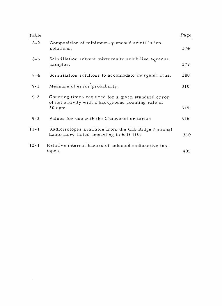
IV OPERATION AND CHARACTERISTICS OF AN INTERNAL - SAMPLE (LIQUID) SCINTILLATION COUNTER 477
THE NATURE OF RADIOACTIVE DECAY 491
VI INTERACTION OF RADIATION WITH MATTER 497
VII STATISTICAL CONSIDERATIONS IN THE MEASUREMENT OF RADIOACTIVITY 508
PART THREE -- SELECTED RADIOTRACER EXPERIMENTS
EXPERIMENT A INCORPORATION OF C1402 INTO AMINO
ACIDS IN YEAST 511
B A KINETIC STUDY OF THE UTILIZATION OF GLUCOSE -U -C14 BY INTACT RATS BY MEANS OF AN ELECTROMETER SYSTEM 530
C THE EFFECT OF X- IRRADIATION ON BONE MARROW ACTIVITY IN RATS AS MEASURED BY IRON- 59 INCORPORATION INTO ERYTHROC YTES
D AN INVESTIGATION OF SODIUM ION REGULATION IN CRAYFISH USING SODIUM -22
E DETERMINATION OF COEFFICIENTS OF ZINC -65 ACCUMULATION IN FRESHWATER PLANTS
547
567
583

LIST OF FIGURES
Figures Page
2 -1 Relation of Nuclear Composition to the Line of Stability. 33
2 -2 Decay Scheme of P32. 38
2 -3 Decay Scheme of Co60. 38
2 -4 Decay Scheme of 1131 38
2 -5 Decay Scheme of N13 39
2 -6 Decay Scheme of Fe55. 40
2 -7 Decay Scheme of Na22. 40
2 -8 Decay Scheme of Rn219. 42
2 -9 Linear Decay Curve. 45
2 -10 Semi - logarithmic Decay Curve. 45
2 -11 Relation Between Half -life and Activity. 50
2 -12 Direct Graphic Determination of Half -life. 52
2 -13 Graphic Resolution of a Composite Decay Curve. 57
3 -1 Diagram of the Nuclear Potential Barrier and "Energy Well" Concept. 69
3 -2 Typical Specific Ionization Curve for Alpha Particles in Air. 72
3 -3 Typical Range Curve for Alpha Particles in Air. 72
3 -4 Range- energy Curve for Alpha Particles in Standard Air. 74
3 -5 Simplified Diagram of a Magnetic Spectrometer. 80
3 -6 Energy Distribution Curve of Beta Particles from P32 81
Figure Page
3 -7 Beta Energy Curves for Several Beta Emitters. 83
3 -8 Specific Ionization Curve for Beta Particles in Air. 87
3 -9 Plot of Absorption of Beta Particles in Matter. 88
3 -10 Beta Transmission Curves for Three Mica Window Thicknesses. 90
3 -11 The Electromagnetic Spectrum on a Logarithmic Energy and Frequency Scale. 94
3 -12 Photoelectric Effect. 98
3 -13 Compton Effect. 99
3 -14 Pair Production. 100
3-15 Gamma Ray Absorption 101
3 -16 Exponential Absorption of Gamma Radiation. 107
3 -17 Mass Absorption Coefficients for Gamma Rays in Lead. 111
3 -18 Relation Between X and Gamma Energy in Various Absorbers. / 113
4 -1 A Simple Ionization Chamber Circuit (Integrating Type). 125
4 -2 The Relationship of Ionization Current to Ion Chamber Potential. 129
4 -3 Diagram of a Lauritsen Electroscope. 131
4 -4 Relation of Pulse Size to Potential Gradient in an Ionization Chamber. 137
4 -5 Common Forms of Proportional Detectors. 146
4 -6 Characteristic Curve for a Proportional Detector. 148
4 -7 Various Forms of G -M Detectors. 151
2
Figure
4 -8
5 -1
Page
Characteristic Curve for a G -M Detector. 155
Diagram of a Typical Solid Fluor External Sample Scintillation Detector. 163
5 -2 Theoretical and Actual Gamma Ray Spectra for Co60
5 -3 Comparison of Emission Spectra of Na I (T1) and Anthracene with the Spectral Sensitivity of an Sb- Cs Alloy Photocathode with S -11 Response.
171
177
5 -5 Effect of Amplifier Gain on Counting Rate for a Na I (T1) Scintillation Counter. 180
5 -6 Calculated Gamma Detection Efficiency as a Func- tion of Gamma Energy for a 1" x 1" Na I (Ti) Cry- stal with Sources Directly on Crystal.
6 -1 Spectral Relations Between Primary and Secondary Solutes (in Toluene Solvent) and Photocathode Sensi- tivity.
182
190
6 -2 An Idealized Beta Pulse Spectrum. 216
6 -3 The Effect of Increasing Photomultiplier Gain on the Shape of the Observed Beta Spectrum. 216
6 -4 Balance Point Operation -- Effect of Spectrum Shift 218
6 -5 Balance Point Determination -- Effect of Window Width on Count Rate. 218
6 -6 Pulse Spectra of C14 at Different Photomultiplier Gain Settings. 219
6 -7 Procedure in Preparing a Quench Correction Curve by the Pulse Height Shift Method. 223
8 -1 A Modified Van Slyke -Folch Apparatus for Wet Combustion of C14- labelled Samples. 258

Figure Page
9 -1 A normal distribution curve. 309
9 -2 Factors in G -M radiotracer assay. 318
9 -3 Geometry of an end -window G -M detector 321
9 -4 Resolving time of a G -M detector 327
9 -5 The effect of beta energy and backing thickness on backscatter. 332
9 -6 Saturation back scattering factor in relation to the atomic number of the backing material. 333
9- 7 Correction for f by means of an extrapolated absorption curvé 336
9 -8 Self- absorption curve for samples of constant specific activity. 338
9 -9 Self- absorption curve for samples of constant activity. 338
9 -10 A typical self- absorption correction curve. 341
10 -1 Time -course plot of radiochemical recovery in CO2 from Acetobacter suboxydans metabolizing specifi- cally labeled glucose. 371
13 -1 Floor Plan for Typical Modular Radioisotope Laboratory for Low Level Studies 433
13 -2 Isometric View of Typical Modular Radioisotope Laboratory for Low Level Studies 434
Experiment Figure
I-1 Block diagram of a Geiger -Mueller counter assembly 442
II -1 Block diagram of a proportional counter assembly 456
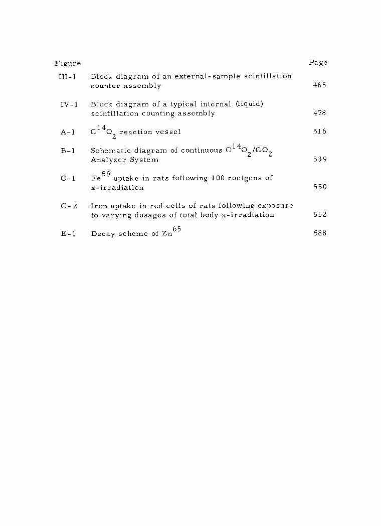
Figure Page
III-1 Block diagram of an external-sample scintillation counter assembly 465
IV -1 Block diagram of a typical internal (liquid) scintillation counting assembly 478
A -1 C14O2 reaction vessel 516
B -1 Schematic diagram of continuous C14 02/CO2 Analyzer System 539
C -1 Fe59 uptake in rats following 100 roetgens of x- irradiation 550
C- 2 Iron uptake in red cells of rats following exposure to varying dosages of total body x- irradiation 552
E -1 Decay scheme of Zn65 588

LIST OF TABLES
Table Page
1 -1 Neutron -proton combinations for hydrogen and carbon. 16
1 -2 Relative natural abundance of the stable isotopes of several elements of biological importance. 19
2 -1 The relation of half -life and beta particle energy to stability for isotopes of carbon and sodium. 35
2 -2 Decay constants for selected radioisotopes. 46
2 -3 Decay correction table for phosphorus -32. 49
2 -4 Half -life values for some selected radioisotopes. 54
2 -5 Average life values for some selected radioisotopes. 59
2 -6 Price and specific activity of calcium -45. 64
3 -1 Linear range of seven Mev alpha particles in some common absorbers. 75
3 -2 Equivalent thickness in mg /cm2 for seven Mev alpha particles of some common absorbers. 76
3 -3 Linear absorption coefficients per cm for selected absorbers. 103
3 -4 Mass absorption coefficients in cm2 /g. 105
4 -1 Average energy lost by 5 Mev alpha particles in producing one ion pair in some common gases. 123
5 -1 Properties of some common fluors. 173
6 -1 Summary of radiation detector characteristics. 226
8 -1 Sample preparation required for various radiation counter types (for beta -emitting samples) 253
Table
8 -2 Composition of minimum -quenched scintillation solutions.
Page
274
8 -3 Scintillation solvent mixtures to solubilize aqueous samples. 277
8 -4 Scintillation solutions to accomodate inorganic ions. 280
9 -1 Measure of error probability. 310
9 -2 Counting times required for a given standard error of net activity with a background counting rate of 30 cpm. 315
9 -3 Values for use with the Chauvenet criterion 316
1 1 - 1 Radioisotopes available from the Oak Ridge National Laboratory listed according to half -life 380
12 -1 Relative internal hazard of selected radioactive iso- topes 405
RADIOTRACER METHODOLOGY IN BIOLOGICAL SCIENCE
INTRODUCTION
The detonation of the first nuclear weapon on the New Mexico
desert in July, 1945, marked the beginning of the nuclear age. Al-
though military development of nuclear weapons continues, since the
end of World War II peaceful uses of nuclear energy have multiplied at
a very rapid pace, These uses include not only the more impressive
employment of nuclear reactors for power generation, but the develop-
ment of a wholly new methodology concerned with the utilization of
some of the by- products of nuclear fission reactors - -- radioisotopes.
The use of radioisotopes in industrial processes and as a re-
search tool can be generally classified into four major categories on
the basis of the respective properties of the radioisotopes that are uti-
lized. These categories are (1) Uses based on the effect of ionizing
radiation on matter; (2) Uses based on the effect of matter on ionizing
radiation, i_e. , the absorption of ionizing radiation by matter; (3) Age -
dating based on the radioactive decay of certain natural radioisotopes;
(4) The use of radioisotopes to trace the fate of stable isotopes in
physical or biological processes,
With the first type of radioisotope technology, use is made of
the high level of energy associated with nuclear radiation, particularly
gamma radiation. The magnitude of energy associated with nuclear
2
radiation derived from radioisotopes, such as radioactive cobalt or
radioactive cesium, is such that it can induce chemical reactions or
disrupt biological functions. Thus, gamma irradiation in varying
doses is commonly employed at present in polymer manufacture, can-
cer therapy, and food sterilization. In this type of application, the
important consideration is the availability of a massive dose. The
chemical identity of the isotope used is of little importance here, as
long as the desirable amount of radiation energy is provided.
The second category of radioisotope technology takes advantage
of the characteristic interaction of ionizing radiation with matter.
Such interaction results in the absorption of a defined amount of the
energy associated with nuclear radiation by a given type of matter of a
given thickness. Similarly, the back - scattering of ionizing radiation
by matter is also related to the nature and thickness of the matter.
This relation has been used effectively in the devising of various types
of industrial thickness gauges. Most such thickness gauges involve
the use of small amounts of beta emitters and occasionally some soft
gamma emitters.
The basic principle underlying the age- dating method is the
defined half -life that is a distinctive characteristic of each radioiso-
tope. Use is made of the presence in the natural environment of a
number of naturally occurring radioisotopes such as uranium -238,
3
carbon-14, and hydrogen -3. In the case of carbon -dating, the carbon -
14 content of living matter is in equilibrium with that in the atmos-
phere in the form of C1402. After the death of any living matter, such
as a tree, the C14 in its remains ceases to maintain equilibration with
atmospheric C14, and hence the C14 content will continuously decline
at a defined rate determined by the half -life of C14. If one analyzes
the C14 content in a piece of an ancient timber, for example, one can
fairly accurately calculate the age of the specimen by comparing this
determined value with the C14 content in the atmosphere. The devel-
opment of age- dating methods has very much benefited the field of
archaeology in recent years (9, Chapter 1).
The use of radioisotopes as tracers has provided research
workers with a powerful new tool. Not only can the fate of a given
compound in either physical or biological processes be readily traced
by the use of radioactively labeled compounds, but the means of assay-
ing radioactivity make possible detection of an extremely minute
amount of a given labeled compound in a given sample. The magnify-
ing power of an operation of this type is estimated to be several magni-
tudes higher than such modern devices as the electron microscope.
This tracer function has manifold biological, chemical, and industrial
applications. In the present text the scope is restricted primarily to
the application of radiotracers to research in the biological sciences.
4
The value of this powerful research tool can be illustrated by
the accomplishments of Calvin and his co- workers at the University of
California in the study of photosynthetic mechanisms. The fate of CO2
in the photosynthetic process has long been a mystery and had defied
many earlier research endeavors. Using radioactive CO2, i. e. ,
C1402, as a tracer, Calvin's group was able to elucidate the complete
fate of atmospheric CO2 in plants leading to the formation of glucose
and other carbohydrate end -products.
In order to make adequate use of the radioisotope method as a
research tool, one needs to possess a good understanding of certain
basic concepts involved in radiotracer experiments. The characteris-
tics of radioactive isotopes and the ionizing radiation they emit must
be comprehended. The detection of radioactivity also constitutes a
basic facet of radiotracer methodology since proper instruments and
procedures have to be selected for a given experiment. This is a
particularly difficult task inasmuch as the advances in nuclear instru-
mentation have been following a very rapid pace in recent years.
Proper experimental design is also a prerequisite in obtaining
reliable results in any radiotracer experiment. Acquiring such a
background in nuclear physics, radiochemistry, and electronics
through formal course work, in addition to gaining the required depth
and breadth in his own field, often works a hardship on the researcher
2

5
in the biological sciences. The intended purpose of this text is to pre-
sent a summary of the essential and pertinent information needed by
such individuals. The content has been chosen on the basis of courses
in radiotracer methodology in the biological sciences taught at Oregon
State University for many years to senior undergraduates, graduate
students, and research workers.
This book is in no way intended as a reference or source book
in the field. Rather it attempts to set forth only the most basic con-
cepts of radioactivity necessary to the practical use of radiotracers.
Nevertheless, it ranges from a coverage of the older techniques, such
as the use of the Geiger- Mueller counter for beta assay, up to such
current techniques as liquid scintillation counting of tritium labeled
compounds. Thus, it is primarily intended as a brief, but up -to -date
introduction to the field of radiotracer methodology. It has been devel-
oped with a formal course sequence in mind, but should prove equally
valuable to the established biological investigator who desires to famil-
iarize himself with this field.
In view of the introductory character of this book, it was deem-
ed especially important to include a rather comprehensive bibliogra-
phy. The interested reader can thus readily find the additional infor-
mation concerning theory and technique that he may require, without
the text itself taking on an encyclopedic nature. References are
6
grouped by text chapters and further subdivided into major topics.
Other general texts concerning radiotracer methodology in general are
listed in the appendix. Since references to older techniques are thor-
oughly covered in these texts, it was felt that the bibliography in the
present book should stress the more recently developed and currently
used radiotracer methods. To this end, a most comprehensive biblio-
graphy of liquid scintillation detection and sample preparation techni-
ques, as well as tritium labeling methods is included.
The presentation is divided into three major divisions: (1) the
text proper, covering primarily the principles, (2) a set of basic ex-
periments concerned with procedures in detecting and characterizing
radioactivity, and (3) an additional set of selected experiments illus-
trating typical radiotracer applications in the biological sciences. The
first and largest division lays the foundation of essential information
regarding the nature of radioactive isotopes and ionizing radiation. It
further describes in detail various means of detecting the radiation
from radiotracers. A practical coverage is also included of the pre-
paration of biological samples for radioactivity assay, the sources of
error in such assay, radiation safety precautions to be observed,
proper design of radiotracer laboratories, and the availability of iso-
topically labeled compounds.

7
The most salient feature in this first section is the discussion
of proper experimental design in radiotracer research. The author
feels this to be one of the most vital, but commonly overlooked aspects
of experimental work with radiotracers. The question, "How much
isotope shall I use ? ", is ultimately asked by every worker approach-
ing an experiment involving radiotracers. Guide lines are presented
to help answer this question and the related one concerning specific
activity. As illustrations, these principles of design are applied in a
step -by -step manner to several of the selected tracer experiments
found in the last section of the book.
The second division of this volume is made up of a set of basic
experiments. These are designed to familiarize the student with the
operation and characteristics of the most commonly used radiation
counting assemblies. Particular attention is given to comparing the
distinctive features of these counters as a basis for selecting the cor-
rect counting assembly for a given detection task. Stress is also
placed on deriving meaningful data from the counters by recognition
and correction of sources of counting errors. Some of the fundamen-
tal characteristics of radiation, such as half -life and absorption by
matter, are also considered on an experimental basis.
A carefully chosen group of applied radiotracer experiments
forms the last division of the book. These experiments were selected

8
to illustrate a diversity of research applications in various fields of
biological science. They involve such varied functions as ion uptake,
red blood cell synthesis, and carbon dioxide incorporation. Further-
more, they utilize a wide range of organisms including mammals, in-
vertebrates, plants, and microorganisms. The experiments were
chosen to employ a variety of radioisotopes - -- Fe59, C14, Zn65,
Na22 - -- with a broad span of decay types and energies. Such a span
requires, of course, the use of several different detector types.
In general, these applied experiments are intended to be on the
level of course term projects. As employed in courses at Oregon
State University, such projects occupy the last month of the students'
laboratory time. Inspection will show that they were adapted from
original research efforts. With the class -time factor in mind, the
original procedures were simplified and the statistical sampling neg-
lected. Ample citations of the original literature are given with each
experiment to allow further pursuit of the problem as an advanced re-
search project at the professor's discretion.
It is the author's sincere hope that this book will serve as a
key to open the door to the utilization of radiotracer techniques for
many a hopeful or experienced biological scientist. Although brilli-
antly exploited over the past two decades, the methodology has only

9
begun to shed light into some of the dark corners of our present ignor-
ance.

PART ONE
PRINCIPLES OF RADIOTRACER METHODOLOGY
10
CHAPTER 1 - ATOMS AND NUCLIDES
It is highly important to first understand the physical nature of
radioactive isotopes in order to use them advantageously as tracers in
the study of biological functions. While a detailed knowledge of nu-
clear physics may not be necessary, it is at least essential to compre-
hend some of the general concepts. Toward this end, it is advisable
to briefly and simply review some of the basic information on atomic
and nuclear structure before discussing radioactive isotopes as such.
For readers well versed in the physical sciences this may be unneces-
sary, but for many whose formal training is largely in the biological
sciences, it should prove a valuable review. The reader is referred
to the general references at the end of this chapter for a more detailed
discussion of the physical aspects of radioactive isotopes covered in
the first three chapters of this book.
A. General Structure of the Atom
The present concept of the nature of matter has been largely
developed over the past century. It views all matter as ultimately di-
visible into infinitesimal units known as atoms. Atoms themselves, of
course, are further divisible into yet smaller sub -units. The more
massive particles, such as neutrons and protons, are arranged in the

11
atom to form an extremely dense and positively charged nucleus, sur-
rounded by from one to over one hundred negatively charged electrons.
These electrons move about in statistically determined orbits of vary-
ing distance from the nucleus. o
Generally speaking, atoms have radii of the order of 1 A. The
o dense nuclei have radii of the order of 0. 0001 A, while the radius of
o orbital electrons is of the order of 0. 00002 A. Such dimensions are
well below even the best resolving powers obtainable with the electron
microscope. From these figures it is evident that the nucleus occu-
pies only a minute fraction of the volume of the atom. Thus, atoms
are essentially empty space, crudely like minuscule solar systems.
The physical characteristics of an atom are related to its total
structure, including both the nucleus and the orbital electrons. Chem-
ical behavior, on the other hand, is governed by the number and ar-
rangement of orbital electrons, while the phenomena of radioactivity
are related only to the nuclear composition of atoms. The energy
change associated with orbital electrons during a chemical reaction is
relatively small. In comparison, the nuclear energy changes associ-
ated with radioactivity are very large indeed.
In order to discuss quantitatively these energy differences, a
specific unit of energy measurement must be considered here. This
unit is the electron volt (ev). The electron volt is equivalent to the

12
kinetic energy an electron would acquire while moving through a po-
tential gradient of one volt. Since the electron has very small mass
(9 x 10 -28 gm), this is an exceedingly small energy unit. For this
reason, several larger units are more commonly used. These are the
kilo electron volt (Kev), the million electron volt (Mev), and the bil-
lion electron volt (Bev). The electron volt may also be expressed in
the more familiar energy unit of calories. One electron volt is equi-
valent to 3. 85 x 10 -20 calories.
With reference to these energy units, it can be stated that the
energy range of chemical reactions involving orbital electrons is of
the magnitude of 10 ev per atom, while the kinetic energy of individual
gas molecules in ordinary room air is only a few hundredths of an
electron volt. On the other hand, nuclear changes associated with
radioactivity involve energies on the Key to Mev levels per atom.
Furthermore, to illustrate the true magnitude of nuclear reactions, it
can be calculated that the energy released in the complete radioactive
transformation of a gram atom of radon (atomic weight 222) to polo-
nium (atomic weight 218) would amount to well over 1011 calories.
This is many orders of magnitude larger than the largest values ever
found for heats of chemical reactions.
B. The Nucleus
13
Atomic nuclei are currently believed to be composed of two
major components, namely protons and neutrons. The collective term
for these is nucleons. Protons are positively charged particles, with
a mass approximately eighteen hundred fifty times greater than that of
an orbital electron. Protons must not be thought of as immobile par-
ticles. Although they are not moving through the relatively large or-
bits of the electrons, they do have a significant angular momentum of
their own.
It will be obvious that to maintain electrical neutrality in the
atom, the number of protons must equal the number of orbital elec-
trons. Thus the number of protons is indirectly related to the chemi-
cal properties of an atom. This number of nuclear protons is equiva-
lent to the atomic number of the elements or symbolically the "Z"
value. Proton numbers run from one for hydrogen, up to 103 for
lawrencium, the most recently produced element. The term element
thus means a group of atoms with the same nuclear proton number.
For example, atomic nuclei with six protons and various numbers of
neutrons, are called carbon atoms, or, if the protons number fifty -
three, the element is known as iodine.
14
Neutrons, the other type of nucleon, carry no electrostatic
charge. Their mass very nearly equals that of the proton. The num-
ber of protons plus neutrons (nucleons) equals the mass number of the
atom, or symbolically, the "A" value. Common hydrogen atoms, for
example, contain only one nucleon, a proton, and therefore, have a
mass number of 1. Common carbon atoms, containing six protons
and six neutrons, will have a mass number of 12. Because neutrons
do not affect the atomic number, they do not alter the chemical pro-
perties of an atom. Thus, for a given element the number of neutrons
may vary within limits. Carbon atoms, for example, all have six
protons and six electrons, but their neutron number may vary from
four through nine. All six of these types of atoms would be chemically
similar, but obviously the nuclei differ drastically in composition.
The term isotopes (from the Greek, meaning "same place ")
means atoms that contain the same number of protons but varying
numbers of neutrons. In other words, they are atoms of the same
atomic number (Z value), but differing mass numbers (A value). The
number of isotopes for each element varies quite widely. It ranges
from hydrogen with three isotopes to tin with twenty- three. In general,
the lighter elements tend to have fewer isotopes than those of higher
atomic number.

15
C. Nuclides and Isotopes
It will be clear now that to merely refer to a given atom as of a
certain element does not describe it with sufficient precision. Its
exact nuclear composition must be specified. This concept is embod-
ied in the term nuclide. There are today approximately 1500 known
nuclides, that is, specific nuclear species. As a biological analogy,
it can be said that the relation between element and nuclide corre-
sponds roughly to the relation between the classification levels of
genus and species, respectively.
Symbolically, a specific nuclear species is represented by a
preceding subscript number for the atomic number, then the alphabe-
tical symbol for the element, followed by a superscript number repre-
senting the mass number. An example is 6C14, which is seen to be an
isotope of the element carbon with a mass number of 14. Since the
symbol for the element determines the atomic number, it is common
to omit this number and to write the preceding simply as C14.
Based on this information, it would seem that any number of
neutrons could be associated with the fixed number of protons in a
nucleus to produce an indefinite number of isotopes of an element with
the same chemical properties. Actually, this is not the case. Only a
relatively few combinations persist in nature. These are known as
16
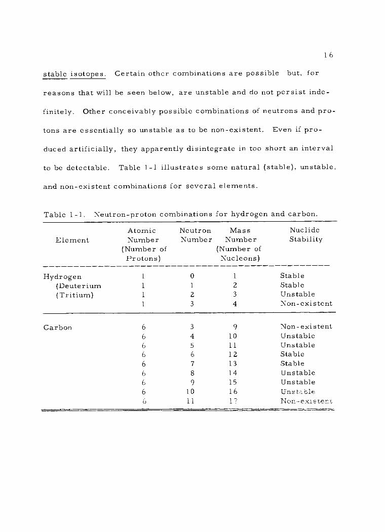
stable isotopes. Certain other combinations are possible but, for
reasons that will be seen below, are unstable and do not persist inde-
finitely. Other conceivably possible combinations of neutrons and pro-
tons are essentially so unstable as to be non- existent. Even if pro-
duced artificially, they apparently disintegrate in too short an interval
to be detectable. Table 1 -1 illustrates some natural (stable), unstable,
and non -existent combinations for several elements.
Table 1 - 1 . Neutron -proton combinations for hydrogen and carbon.
Element
Hydrogen (Deuterium (Tritium)
Atomic Number
(Number of Protons)
1
1
1
1
Neutron Number
0
1
2
3
Mass Number
(Number of Nucleons)
1
2
3
4
Nuclide Stability
Stable Stable Unstable Non - existent
Carbon 6 3 9 Non -existent 6 4 10 Unstable 6 5 11 Unstable 6 6 12 Stable 6 7 13 Stable 6 8 14 Unstable 6 9 15 Unstable 6 10 16 Unstable
11 17 Non -existent ú
17
D. Stable Nuclides
The number of stable nuclides varies widely from element to
element. The element uranium, for example, has no stable nuclear
species. Others, such as sodium, have only one stable nuclide.
From this point the range extends up to a maximum of ten stable iso-
topes for tin. The total number of stable nuclides for all the elements
lumped together is approximately 280. The natural elements found in
the earth's crust or atmosphere are not homogeneous, but are corn -
posed of mixtures of the stable isotopes of each element. For any
given element, the relative proportion of stable isotopes is remarkably
constant, regardless of the geographic locality from which samples
come. The one exception to this rule is the element lead, whose iso-
topic composition varies according to its origin, as will be seen below.
The chief reason that the atomic weights of chemistry some-
times vary widely from whole numbers is that the elements they repre-
sent are not pure nuclides, but often mixtures of several isotopes of
varying mass number. Where several stable isotopes of an element
exist, the atomic weight of that element represents an average calcu-
lated from their percent composition and the mass number (A value) of
the individual isotopes. Chlorine, for example, has an atomic weight
of 35. 457. It can be seen how this is derived when it is noted that two
18
stable isotopes of chlorine exist in nature. The one, chlorine - 35
makes up 75. 53 percent of the element, while the other, chlorine - 37,
makes up only 24. 47 percent. Thus, the atomic weight takes into ac-
count these two percentages and the weights associated with these two
isotopes.
Table 1 -2 indicates the relative abundance of naturally occur-
ring stable isotopes for several of the biologically important elements.
In a number of cases, one stable isotope is much more common than
the others and is considered the "normal" nuclide for that element.
Some examples are Hl C12 N14, X16 Ca40 and 532, which each
account for more than 95 percent of the isotopic abundance of their
element.
All of the reasons for the stability of certain combinations of
neutrons and protons and the instability of others are not fully under-
stood at present. It is clear, however, that stability in general is
based on the ratio of neutrons to protons, although this is not the whole
explanation. The forces tending to nuclear stability are greatest in
those nuclides where the nuclear particles are paired. This principle
can be readily deduced from the following three observations. (1) The
greatest number of stable nuclides - -- about 164 - -- are those which
contain even numbers of both protons and neutrons in the nuclei. (2)
Fewer stable nuclides are found when the number of protons is even,

19
Table 1 -2. Relative natural abundance of the stable isotopes of several elements of biological importance [data from Goldman and Stehn (1961) ] .
Natural Element Nuclide Abundance
Hydrogen H1 99. 985 H2 0. 015
Carbon c12 98. 89 C13 1. 11
Nitrogen N14 99. 63 N15 0.37
Oxygen 016 99. 759 017 0. 037 018 0. 204
Sodium Na23 100 Magnesium Mg24 78. 70
5 10. 13 Mg2 Mg26 11.17
Phosphorus P31 100 Sulfur S32 95. 0
S33 0. 76 S34 4. 22 S36 0. 014
Chlorine C135 75. 53 C137 24.47
Potassium K39 93. 10 K41 6. 88
Calcium Ca40 96. 97 Ca42 0. 64 Ca43 0. 145 Ca44 2. 06 Ca46 0. 0033
Iron Fe54 5. 82 Fe56 91. 66 Fe57 2. 19 Fe58 0. 33
%
20
but the number of neutrons is odd - -- about 55, or when the number of
neutrons is even and the proton number is odd - -- about 50. (3) Nu-
clides with odd numbers of both protons and neutrons number only four
and are restricted to elements with mass number less than 14. These
are rather exceptional cases.
E. Unstable Nuclides (Radioisotopes)
It will be recalled that certain neutron -proton combinations in a
given nucleus are possible, but the resulting nuclide is unstable. Due
to this basic instability, it will sooner or later undergo nuclear
changes. These changes usually result in an adjustment of the neutron -
to- proton ratio so that the nucleus reaches a position of greater stabi-
lity. Such changes in the nucleus will be explored in greater detail in
Chapter 2.
The nuclear changes described involve spontaneous disintegra-
tion of one or more of the nucleons. Such disintegration leads to the
emission of particles or energy from the atom. This type of event is
known as radioactivity, and nuclides possessing it are termed radio-
active nuclides or isotopes. The term is frequently contracted to ra-
dioisotopes. The number of these radioisotopes known today approach-
es 1, 250 and, thus, far exceeds the number of known stable nuclides.
The vast majority of radioisotopes are artificially produced, with only
21
a small minority occurring naturally.
1. Naturally occurring radioisotopes
There were probably many radioisotopes formed at the time of
the earth's creation, which do not occur naturally today. These were
such unstable nuclides that they have long since decayed to stable
forms. Those originally formed radioisotopes which still appear today
are either nuclides that decay very slowly, or those which are mem-
bers of decay series. By the latter term is meant unstable nuclides
which decay to other unstable nuclides, reaching stability only after a
dozen or more such decay steps. Such nuclides are always of high
atomic number.
The three decay series whose member nuclides occur in the
earth's crust are as follows: the uranium - radium series, in which
U238 decays through fourteen intermediates to stable Pb206; the ac-
tinium series in which U235 decays through a series of eleven inter-
mediate nuclides to stable Pb207; and the thorium series in which
Th232 decays through a series of ten intermediates to stable Pb208.
In passing it will be noted that the stable end nuclide of each of these
natural decay chains is an isotope of lead, but a different isotope in
each case. This is an explanation of the observation above that the
isotopic composition of naturally occurring lead varies with the
22
locality from which samples are taken. Thus, lead in a deposit de-
rived largely from decay of the actinium series will differ in percen-
tage composition of isotopes from a sample derived largely from decay
of the thorium series.
Of the originally formed natural radioisotopes of lower atomic
number only one is biologically significant - -- K40. Due to the gen-
eral solubility of potassium compounds, this nuclide is quite widely
distributed in both the earth's crust and bodies of water. Even more
significant is the fact that potassium is a common constituent of living
tissue. This means that a small, but measurable amount of K40 is
present in all living tissue. An average 160 lb. man, for example,
will contain about O. 031 gm of K40 in his body, which amounts to
O. 012 percent of all the K present. These factors make K40 a signifi-
cant contributor to the "background" radiation to which all living things
are constantly exposed.
Other radioisotopes decay too rapidly to have remained since
the time of creation. A few, however, are being continually produced
in the earth's upper atmosphere due to cosmic ray bombardment of at-
mospheric atoms. In the case of these nuclides the constant produc-
tion has reached an equilibrium with the rate of decay, so that their
amount is relatively constant in the natural world.
Tritium (H3) is one of the nuclides being constantly produced.
23
When the nuclei of N14 atoms are struck by neutrons, the resultant
unstable atom may break up into tritium and C12. Such bombarding
neutrons are derived from cosmic ray interaction with other atoms in
the upper atmosphere. Alternatively an unstable N14 -plus- neutron
combination may eject a proton and become a C14 atom. Thus, either
H3 and C14 can be produced as a result of cosmic ray interaction with
N14. The H3 so formed combines readily with oxygen atoms in the
vicinity and slowly descends to the surface of the earth in the molecu-
lar form of water. Likewise, the C14 quickly combines with nearby
oxygen atoms to form radioactive C1402. Both of these radioactive
molecules are readily incorporated into living organisms.
During the life of an organism there will be a rather constant
ratio between the C14 and the C12 in its living tissue. Radiocarbon, or
C14 dating is based on the fact that this constant ratio during life be-
gins to shift after death. Since following the death of the organism no
further C14 is incorporated into the tissues, the amount of C14 present
steadily declines as the unstable nuclei disintegrate. Thus, by deter-
mining the ratio of C14 to C12 in an ancient timber, for example, it
may be calculated how long radioactive decay has been occurring since
the tree from which it came was cut. Libby (9) describes this tech-
nique in detail.
-
24
2. Artificially produced radioisotopes
The first artificial production of radioisotopes was not effected
until 1934, when Curie and Joliot transformed A127 to P3°. In the in-
tervening three decades since that time, hundreds of unstable artificial
nuclides have been formed. This has amounted essentially to the
transmutation of elements - -- the long sought goal of the medieval al-
chemists.
The basic principle for inducing nuclear transformations com-
monly involves the bombardment of stable nuclei with various parti-
cles, either charged or uncharged. This bombardment brings about
temporary imbalance in the target nuclei, usually resulting in the ejec-
tion of nuclear particles or the emission of electromagnetic radiation,
and the resultant formation of a new nuclear species. Many such nu-
clear reactions have been investigated by nuclear physicists. The two
types most important in the production of radioactive tracers involve
the use of various charged particles and uncharged neutrons.
a. By particle accelerators: In order for charged particles to
actually enter and interact with the target nucleus, they must have suf-
ficient kinetic energy. Particles lacking the requisite energy would be
merely repelled or deflected by the energy barrier of the nucleus.
Various particle accelerating devices have been developed to impart
25
sufficient energy to the various bombarding particles. In general
these devices produce stepwise acceleration of the charged particles
by means of a changing magnetic field. One can divide particle accel-
erators into two groups. Linear accelerators accelerate particles in
a straight line, while the particles follow a circular path in such ma-
chines as the cyclotron, betatron, or synchrotron. Such devices can
accelerate particles up to the Mev and Bev level.
Many types of charged particles, such as electrons, protons,
deuterons (deuterium nuclei - -- one proton and one neutron), or alpha
particles (helium nuclei - -- two protons and two neutrons), have been
used. A typical reaction is that in which Mg24 is exposed to a beam of
deuterons and the excited nuclei respond by ejecting an alpha particle
each and being transformed to Na22. Such a reaction would be shown
symbolically as Mg24 (d, a) Na22. In this means of representation the
original nuclide is shown first, then in parenthesis first the impinging
particle, followed by the ejected particle, and finally the resultant nu-
clide. Some other similar typical reactions follow: B10(d, n)C11;
Mg26( a, 2p) Mg28; P31 (a, n) 0.34.
The deuteron is the most useful of all the charged particles
listed above in bringing about transmutation. This is due to many rea-
sons, some of them having to do mainly with the technical processes
of operating accelerators. Perhaps the greatest point in favor of

26
deuteron bombardment is that the deuteron is a rather loose combina-
tion of a proton and a neutron. As such, it may become partially po-
larized in the nuclear force field. The proton may be repulsed, while
the neutron slips into the nucleus to interact. Thus, the neutron may
be captured by the nucleus without the entire deuteron entering the nu-
cleus. This occurs at energy levels far lower than required for cap-
ture of the entire deuteron. In other words, deuteron bombardment
affords a relatively easy process of adding neutrons to the nucleus.
This reaction is known as the Oppenheimer - Phillips process after its
two discoverers. It should be noted here that uncharged neutrons have
a much greater efficiency for interacting with nuclei than the charged
particles.
b. By nuclear reactors: A direct and more massive source of
neutrons for inducing nuclear transformations is found in the atomic
pile, or nuclear reactor. Since reactors were first built during World
War II, they have rapidly taken over as the primary producers of ra-
dioisotopes commonly used for biological purposes. In the early
years of their development in this country, nuclear reactors were en-
tirely controlled by the United States Atomic Energy Commission and
most radioisotopes were produced at the Oak Ridge National Labora-
tories in Tennessee. In more recent years many smaller reactors
have come into operation under private control and now form

27
important secondary sources of specific radioisotopes.
In brief, nuclear reactors are devices to control and sustain
fission reactions. In the fission process, atoms of U235, or certain
other heavy elements, after the capture of a neutron, spontaneously
divide into two smaller nuclides of about the same size with the simul-
taneous emission of several highly energetic ( "fast ") neutrons. In
order to sustain the fission reaction it is necessary to slow these ejec-
ted neutrons to "thermal" energies (about O. 025 ev), so that they may
be captured by other U235 nuclei. For this purpose moderating sub-
stances, such as graphite, are present in the nuclear reactor. Such
moderators slow the neutrons, but do not readily capture them.
If a target material of P31, for example, is placed within the
reactor, it will be exposed to a massive flux of thermal neutrons.
Those target nuclei which capture a thermal neutron will be converted
to radioactive P32 by the following reaction: P31 (n, y) P32. Thus,
the typical result of thermal neutron absorption is the emission of a
gamma photon from the excited nucleus, and the resultant nuclide is
the next higher isotope of the target material. Other similar thermal
neutron reactions of importance are: Ca44 (n, y) Ca45; Zn64 (n, y )
Zn65; Co59 (n, y) Co60.
The neutron flux in a reactor will include many neutrons of
higher than thermal energies. Those with over 100 Key energy are
28
termed "fast" neutrons, while those with energies lying between the
thermal and fast levels are known as slow and intermediate neutrons.
Since the capture of such neutrons by a target nucleus greatly in-
creases the energy of the nucleus, such capture is commonly followed
by the emission of a nuclear particle. Some important examples of
reactions of this type would be: Lib (n, a) H3;
2n) C11; C135 (n, p) S35
N14 (n, p) c14; c12 (n,
The likelihood of neutron capture by a nucleus is expressed as
the target area presented by the nucleus to the bombarding neutron.
This is known as the neutron capture cross - section of the nucleus. It
is expressed in units of 10-24 cm2, called "barns" (taken from the ex-
pression "hitting the broad side of a barn "). Neutron capture cross -
sections differ widely from nuclide to nuclide. In addition, cross -
section values for any given nuclide vary according to the energy of
the impinging neutrons. In general, since neutrons are uncharged
particles, the longer they remain in the region of a nucleus (i. e. , the
less their energy), the greater the chance of interaction.
It will be seen that for any given target material in a nuclear
reactor there will be many competing nuclear reactions occurring si-
multaneously as a result of interaction with neutrons of various ener-
gies. Thus, it is necessary to know the relative yields of these com-
peting reactions and to carefully select the proper target materials in
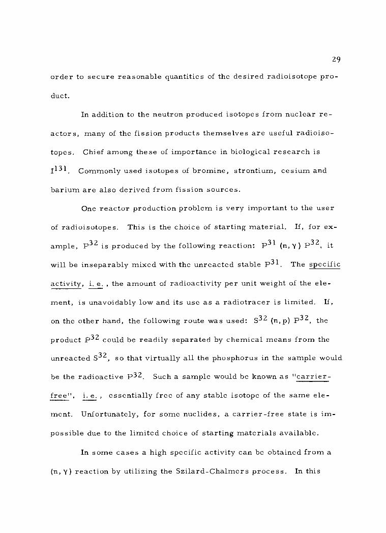
29
order to secure reasonable quantities of the desired radioisotope pro-
duct.
In addition to the neutron produced isotopes from nuclear re-
actors, many of the fission products themselves are useful radioiso-
topes. Chief among these of importance in biological research is
1131 Commonly used isotopes of bromine, strontium, cesium and
barium are also derived from fission sources.
One reactor production problem is very important to the user
of radioisotopes. This is the choice of starting material. If, for ex-
ample, P32 is produced by the following reaction: P31 (n, y) P32, it
will be inseparably mixed with the unreacted stable P31. The specific
activity, i. e. , the amount of radioactivity per unit weight of the ele-
ment, is unavoidably low and its use as a radiotracer is limited. If,
on the other hand, the following route was used: S32 (n, p) P32, the
product P32 could be readily separated by chemical means from the
unreacted S32, so that virtually all the phosphorus in the sample would
be the radioactive P32. Such a sample would be known as "carrier-
free ", i. e. , essentially free of any stable isotope of the same ele-
ment. Unfortunately, for some nuclides, a carrier -free state is im-
possible due to the limited choice of starting materials available.
In some cases a high specific activity can be obtained from a
(n, y) reaction by utilizing the Szilard- Chalmers process. In this

30
process the emission of the gamma photon imparts a recoil momentum
to the product nucleus sufficient to break chemical bonds. Thus the
radioactive atoms produced are in a different chemical form from the
starting material, and are readily separated from it (see Experiment
5).
An additional small -scale source of neutrons is frequently
found in laboratories today. It consists of an alpha emitting substance,
such as radium or polonium, intimately mixed with the light element
beryllium. The alpha irradiation induces the excited Be nucleus to
eject neutrons. The flux of neutron so generated is low compared to
that from nuclear reactors. However neutron sources of this type are
often useful for educational purposes.
BIBLIOGRAPHY
1. Evans, Robley D. The atomic nucleus. New York, McGraw -Hill, 1955. 972 p.
2. Friedlander, Gerhart and Joseph W. Kennedy. Nuclear and radio- chemistry. New York, John Wiley and Sons, 1 955. 468 p.
3. Gamma emitters by half -life and energy. Nucleonics 1 8(1 1 ):1 96- 1 97. 1 960.
4. Glasstone, Samuel. Sourcebook on atomic energy. 2d ed. Princeton, Van Nostrand, 1958. 641 p.
5. Goldman, David T. and John R. Stehn. Chart of the nuclides. Schenectedy, General Electric, 1961. 1 sheet.
3t
6.
7.
Ha1lden, Naorni A. Beta ernitters by energy and half-Iife.Nucleonics I 3(61278-79. 1955.
Kinsrnan, Sirnon (ed. ). Radiological-h€alth handbook. Rev. ed.Washington, U. S. Public Health Service, Division of Radio-logical Health, I960" 468 p"
Lapp, Ralph E. and Howard L. Andrews. Nuclear radiationphysics. 2d ed, New York, Prentice-Ha1l, 1954. 532 p.
Libby, Willard F. Radiocarbon dating" 2d ed" Chicago,University of Chicago Press, I955. 175 p.
Oldenburg, Otto" Introduction to atornic and nuclear physics.3d ed. New York, McGraw-Hill, 1961 . 380 p.
Sernat, Henry. Introduction to atornic and nuclear physics. 4t1aed. New York, Holt, Rinehart and Winston, 196?. 6?8 p.
8.
9.
I0.
tt.
tz" Slack, L. and K. Way. Radiations frorn radioactive atorns infrequent use. Washington, U. S. Atornic Energy Cornrnission,r959. 75 p.
13. Srnith, Gilbert W. and Donald R. Farrnelo. Radionuclides ar-ranged by garnrna-ray energy. Nucleonics l5(2):80-81 . 1958.
I4. Stehn, John F. Table of radioactive nuclid.es. Nucleonics l8(l I ):r 86-l 95. I 960.
I5. Stokely, Jarnes and David T. Goldrnan. Nuclides and isotopes.6ttr ed. Schenectedy, General Electric, 1962. 7 p.
16. Strorninger, D., J. M. Hollander and G. T. Seaborg. Tab1e ofisotopes. Reviews of Modern Physics 30:585 -904. 1958.
17. Su11ivan, 'vVilliarn H. Trilinear chart of nuclides. Washington,U. S. Atornic Energy Cornrnission, I957-196I . 9 p.
CHAPTER 2 - THE NATURE OF RADIOACTIVE DECAY
A. Radionuclides and Nuclear Stability
32
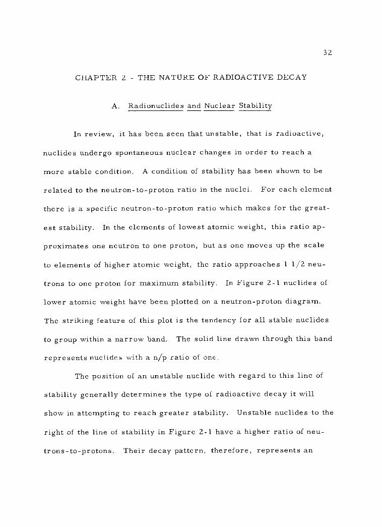
In review, it has been seen that unstable, that is radioactive,
nuclides undergo spontaneous nuclear changes in order to reach a
more stable condition. A condition of stability has been shown to be
related to the neutron -to- proton ratio in the nuclei. For each element
there is a specific neutron -to- proton ratio which makes for the great-
est stability. In the elements of lowest atomic weight, this ratio ap-
proximates one neutron to one proton, but as one moves up the scale
to elements of higher atomic weight, the ratio approaches 1 1/2 neu-
trons to one proton for maximum stability. In Figure 2 -1 nuclides of
lower atomic weight have been plotted on a neutron -proton diagram.
The striking feature of this plot is the tendency for all stable nuclides
to group within a narrow band. The solid line drawn through this band
represents nuclides with a n/p ratio of one,
The position of an unstable nuclide with regard to this line of
stability generally determines the type of radioactive decay it will
show in attempting to reach greater stability. Unstable nuclides to the
right of the line of stability in Figure 2 -1 have a higher ratio of neu-
trons-to- protons. Their decay pattern, therefore, represents an

25 20 15 10
Number of Protons o
Figure 2 -1. Relation of Nuclear Composition to the Line of Stability.
m
o F-1
a)
z t+A
o
1.1)
z
33

34
attempt to decrease the neutron content and /or increase the proton
content. On the other hand, radioactive nuclides to the left of the line
of stability have a higher ratio of protons -to- neutrons. Their decay
pattern then is an attempt to reduce proton content and /or increase
neutron content. Thus, the types of decay that will be described fol-
lowing are directly related to the above problem of nuclear instability.
Certain other radioactive decay characteristics are influenced
by the relative distance of specific nuclides from the line of stability.
In general, for a given element the half -lives (see page 48) of its ra-
dioactive isotopes are inversely related to their distance from the line
of stability. The energy associated with the particles or photons emit-
ted during decay by these isotopes also normally bears a direct rela-
tionship to the distance of the specific nuclide from the line of stabi-
lity. Table 2 -1 illustrates these relations in the case of carbon and of
sodium.
B. Types of Radioactive Decay
A so- called "decay scheme'; is a convenient means of concisely
summarizing information concerning a specific type of radioactive de-
cay. It is a conventionalized plot of energy against atomic number,
although no scale is used. The symbol, mass number, and half -life of
the nuclide appear on the uppermost horizontal line. Decay leading to
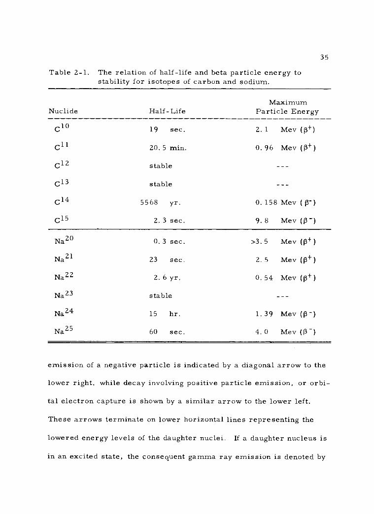
35
Table 2 -1. The relation of half -life and beta particle energy to stability for isotopes of carbon and sodium.
Maximum Nuclide Half -Life Particle Energy
C10 19 sec. 2. 1 Mev (ß +)
C11 20.5 min. 0.96 Mev (p+)
c1-2 stable -
C 13 stable -
C14 5568 yr. 0. 158 Mev (ß-)
C15 2.3 sec. 9. 8 Mev (f3 )
Na20 0. 3 sec. >3.5 Mev (ß +)
Na21 23 sec. 2.5 Mev ((3 +)
Na22 2. 6 yr. 0.54 Mev ((3+ )
Na23 stable -
Na24 15 hr. 1.39 Mev (ß-)
Na25 60 sec. 4. 0 Mev (ß -)
emission of a negative particle is indicated by a diagonal arrow to the
lower right, while decay involving positive particle emission, or orbi-
tal electron capture is shown by a similar arrow to the lower left.
These arrows terminate on lower horizontal lines representing the
lowered energy levels of the daughter nuclei. If a daughter nucleus is
in an excited state, the consequent gamma ray emission is denoted by
-
36
undulating vertical arrows (no change in atomic number) leading to the
ground energy state of the nucleus. Notation of the maximum kinetic
energy in Mev of emitted particles and the energy in Mev of gamma
radiation is made near the respective arrows. Where nuclei may fol-
low more than one decay path, the percentage occurrence of each path
is indicated. Typical decay schemes are shown for the various decay
types on the following pages.
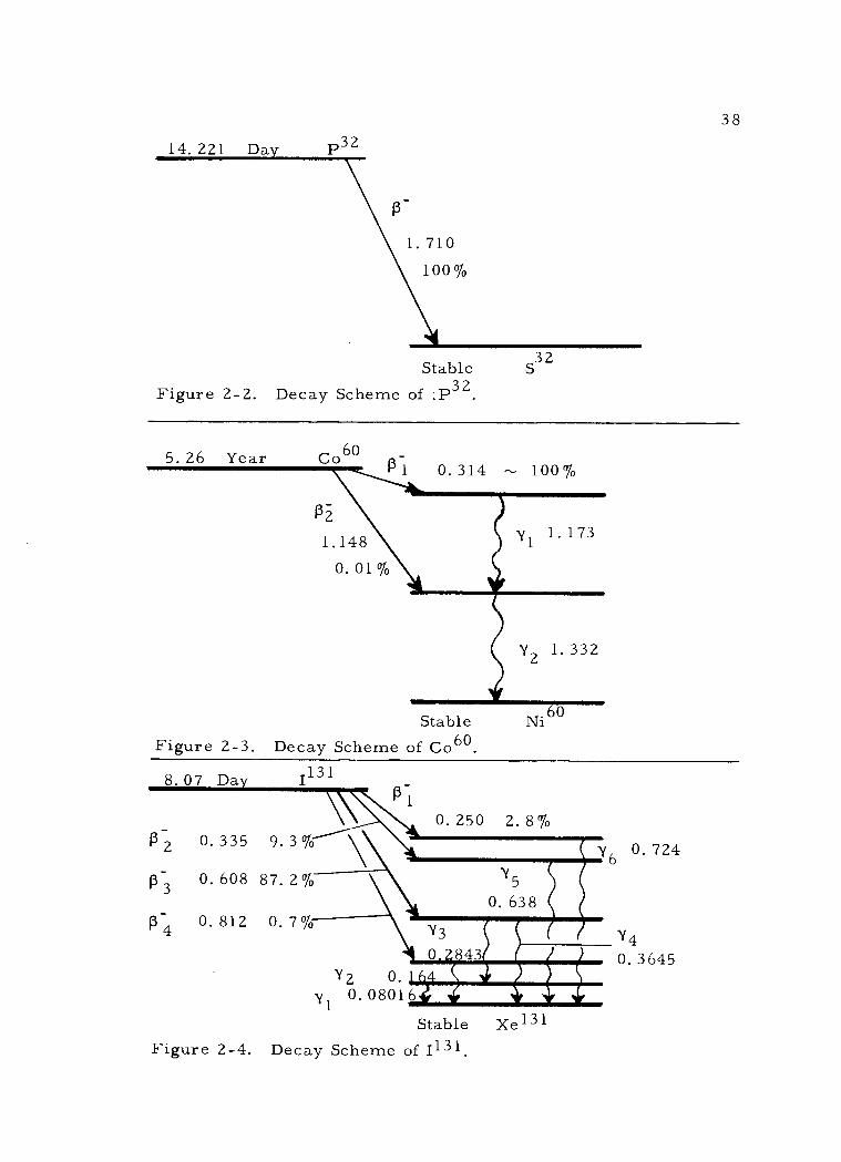
1. Decay by negatron emission
Under certain conditions nuclides with excess neutrons may
reach stability by the conversion of a neutron to a proton accompanied
by the ejection of an electron from the nucleus. Note that this electron
originates in the nucleus and is not to be confused with the orbital elec-
trons. Such a nuclear change results in a loss of one neutron and a
gain of one proton, thus shifting the nuclide toward the line of stability.
Any excess energy in the nucleus following this is emitted as one or
more photons, or gamma rays. Gamma rays are not particulate, but
represent electromagnetic radiation much like x -rays. The electron
ejected from the nucleus is known as a negatron, or a negatively beta
particle. This type of decay can be superficially summarized as fol-
lows: n > p+ + ß- , but see page 84 for a precise presenta-
tion of beta decay.
37
Decay schemes of varying complexity involving negatron emis-
sion are shown in Figures 2 -2, 2 -3, and 2 -4. Close observation of
the decay schemes for Co60 and 1131 will disclose that although two or
more decay paths may be followed, the total disintegration energy to
the stable ground state is essentially a constant value for each respec-
tive nuclide. For Co" this value is 2. 81 Mev and for 1131 it is ap-
proximately 0. 972 Mev. This total disintegration energy to reach the
ground state of the daughter nuclide is known as the "Q value. "
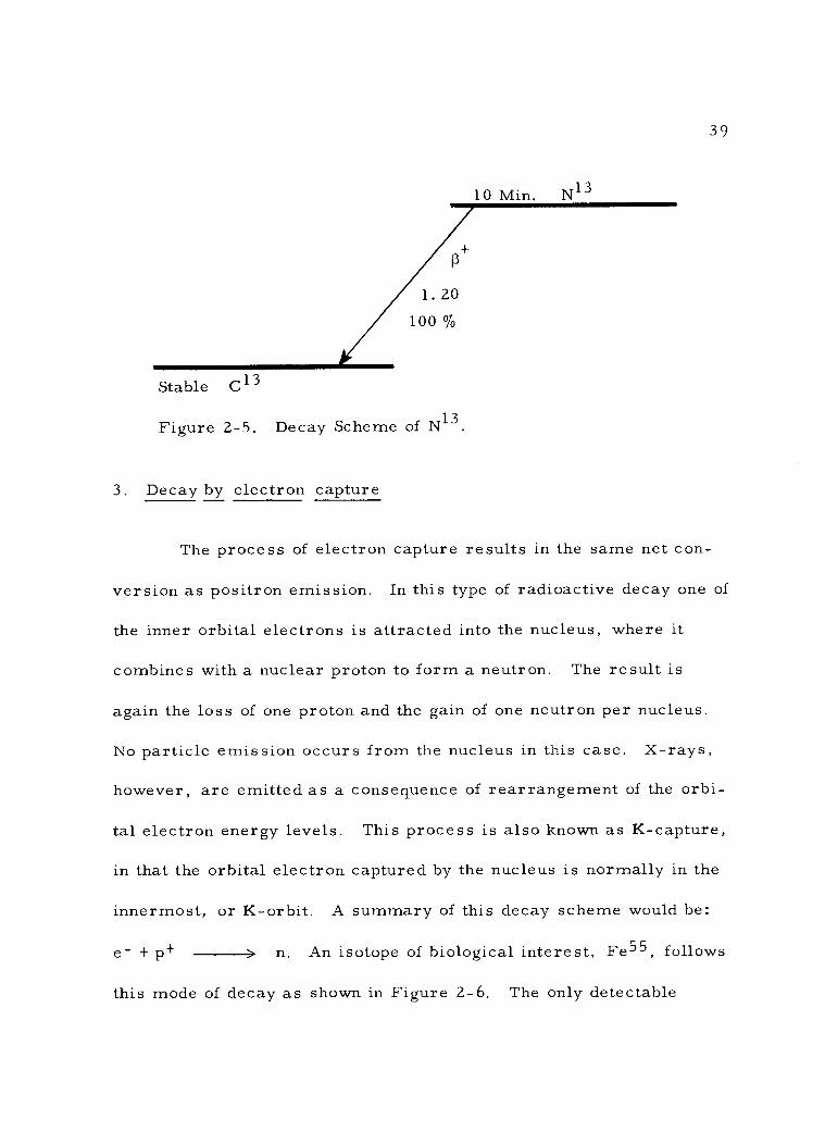
2. Decay by positron emission
Where the number of protons in a nucleus is in excess, posi-
tron emission may occur to reach stability. Positrons are positively
charged beta particles. In this type of transformation a nuclear pro-
ton is converted to a neutron accompanied by the ejection of a high
speed positron from the nucleus. Again, any excess energy in the
nucleus following positron ejection is emitted as gamma radiation.
This reaction may be generally indicated as follows:
p+ ) n + ß+ , but the more refined concept of beta decay
presented on page 84 should be noted. The decay scheme of N13,
shown in Figure 2 -5, illustrates simple positron decay.
38
14.221 Day P32
Stable S 32
Figure 2 -2. Decay Scheme of :P32.
5.26 Year Co60 0.314 -ti 100%
1. 173
Y2 1. 332
Stable Figure 2 -3. Decay Scheme of Co60
8.07 Day 1131
P-2 0.335
P-3 0.608
P-4 0.812
9.3%
87. 2 %
0.7%
0.250 2.8%
Y5
0. 638
Y2 0. y1 0.08016
Y3
I 843 srw'_ 4111111=11M
Stable Figure 2 -4. Decay Scheme of I131
Xe131
0. 724
Y4
0. 3645
\ R
1
Pi 1.148
0.01%
0
Y,
Stable C13
Figure 2 -5. Decay Scheme of N13
3. Decay by electron capture
10 Min. N13
39
The process of electron capture results in the same net con-
version as positron emission. In this type of radioactive decay one of
the inner orbital electrons is attracted into the nucleus, where it
combines with a nuclear proton to form a neutron. The result is
again the loss of one proton and the gain of one neutron per nucleus.
No particle emission occurs from the nucleus in this case. X -rays,
however, are emitted as a consequence of rearrangement of the orbi-
tal electron energy levels. This process is also known as K- capture,
in that the orbital electron captured by the nucleus is normally in the
innermost, or K- orbit. A summary of this decay scheme would be:
e- + p+ ---> n. An isotope of biological interest, Fe55, follows
this mode of decay as shown in Figure 2 -6. The only detectable
loo %
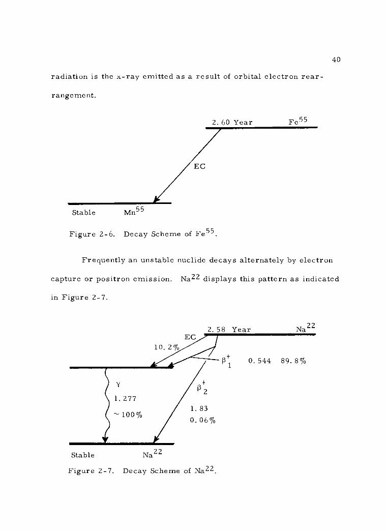
40
radiation is the x -ray emitted as a result of orbital electron rear-
rangement.
EC
Stable Mn55
2. 60 Year Fe55
Figure 2 -6. Decay Scheme of Fe55.
Frequently an unstable nuclide decays alternately by electron
capture or positron emission. Na22 displays this pattern as indicated
in Figure 2 -7.
2. 58 Year
Stable Na22
Figure 2 -7. Decay Scheme of Na22.
Na22
0.544 89.8% R i

41
4. Internal conversion
In modes of decay where gamma rays are emitted from the
nucleus, a given chance exists that an occasional gamma ray will
interact directly with an inner orbital electron in its path. If this
occurs, the energy of the gamma ray is imparted to the electron
which is then ejected from the atom. This event is known as internal
conversion and the emitted electrons are known as conversion elec-
trons. In contrast to the energy spectrum characteristic of negatron
and positron emission (see Chapter 3 ), conversion electrons are
homoenergetic.
5. Isomeric transition
There are some nuclides which decay by gamma ray emission
alone. Of course, this type of decay does not change the number of
neutrons and protons in the nucleus, but is a means of disposing of
excess energy in an excited nucleus. Nuclides of this type are known
as metastable. This process of decay is termed isomeric transition.
6. Decay by alpha particle emission
Among the elements of higher atomic weight only, another
means of decay occurs. This is the emission of alpha particles. An
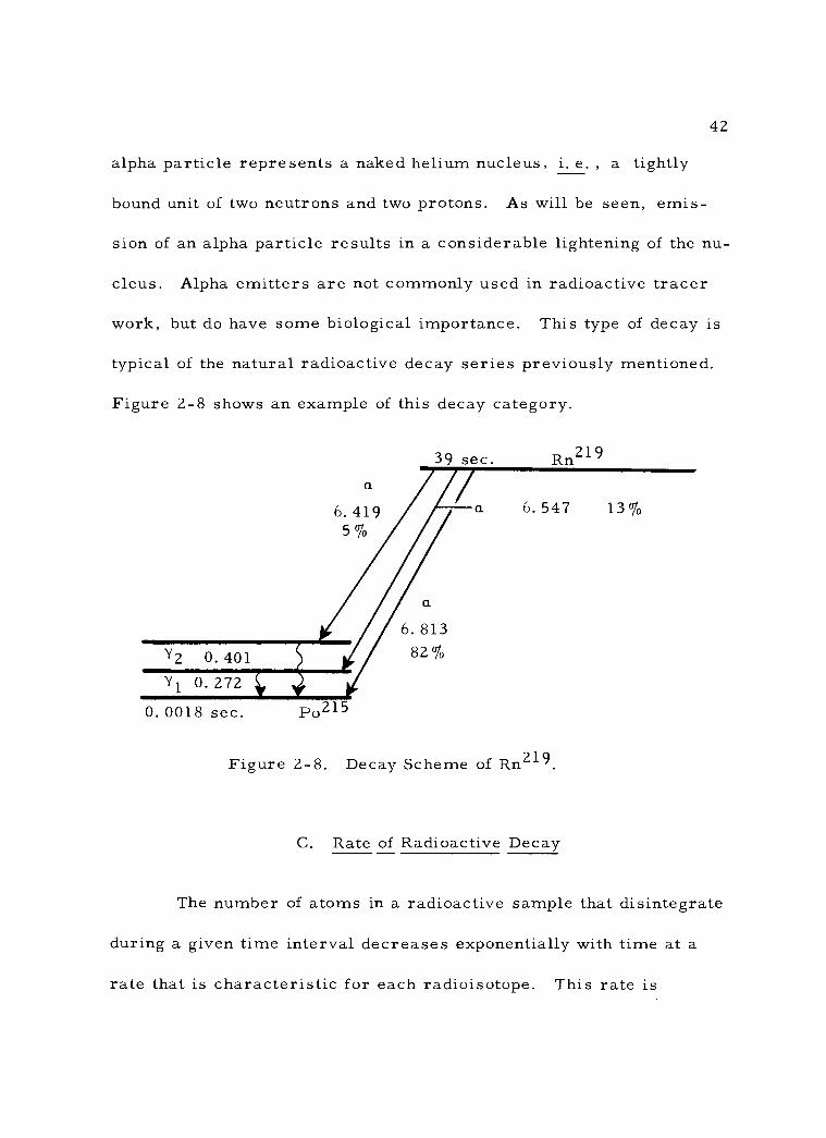
42
alpha particle represents a naked helium nucleus, i. e. , a tightly
bound unit of two neutrons and two protons. As will be seen, emis-
sion of an alpha particle results in a considerable lightening of the nu-
cleus. Alpha emitters are not commonly used in radioactive tracer
work, but do have some biological importance. This type of decay is
typical of the natural radioactive decay series previously mentioned.
Figure 2 -8 shows an example of this decay category.
39 sec. Rn219
0.0018 sec. Po215
Figure 2 -8. Decay Scheme of Rn219
C. Rate of Radioactive Decay
The number of atoms in a radioactive sample that disintegrate
during a given time interval decreases exponentially with time at a
rate that is characteristic for each radioisotope. This rate is
a
6. 419 5%
Y2 0. 401
Y 1 0. 272
a
6. 813 82%
a 6. 547 13%

43
independent of pressure, temperature, the mass action law, or any
other rate - limiting factors that commonly affect chemical and physi-
cal reactions. Thus, this decay rate serves as a most useful means
of identifying a given nuclide. As seen in Table 2 -1, this decay rate
is related to the degree of instability of the specific nuclide. Since
radioactive decay represents the transformation of an unstable to a
stable nuclide, it is an irreversible event for each atom.
The unstable atoms of a given radionuclide do not all decay si-
multaneously. Instead, the decay of a given atom is an entirely ran-
dom event. Because radioactive decay is random, it is possible to
treat it by statistical methods.
1. The decay constant
Thus, one may observe a large number of radioactive atoms
and predict with fair assurance that after a certain time a definite
fraction of them will have disintegrated. This given fraction of atoms
disintegrating in a specific unit of time is the decay constant. The
actual number of radioactive atoms decaying in a certain time period
is not constant, but is dependent on the number of unstable atoms ori-
ginally present in the sample. This relation may be expressed as fol-
lows:
No. atoms decaying No. atoms originally (Equation 2 -1) a in unit time present

44
Note that the above statement shows only a proportion. By introducing
the decay constant, it is possible to convert this expression into an
equation, as follows:
(Equation 2 -2) No. atoms decaying
in unit time
- Decay No. atoms = constant x originally
pre sent
A minus sign must be introduced because the decay leads to a dimin-
ishing of the number of atoms in the sample. Reworking this decay
equation to solve for the decay constant results in:
(Equation 2 -3) No. atoms decaying /in unit time Decay Constant = - No. atoms originally present
In order to convert the word equations above to mathematical
statements using symbols, let N represent the number of atoms of a
radioisotope present at a given time. Then dN represents the number
of atoms which disintegrate in the given time interval dt. The Greek
letter X will represent the decay constant. Using these symbols, the
above three statements will now read as follows:
(Equation 2-4) dN
a N
(Equation 2-5) dt
= - X N
(Equation 2-6) X = -dN/dt or - dN/N
dt
To calculate the value of the decay constant according to Equa-
tion 2 -6, it is necessary to determine the number of radioactive atoms
N '
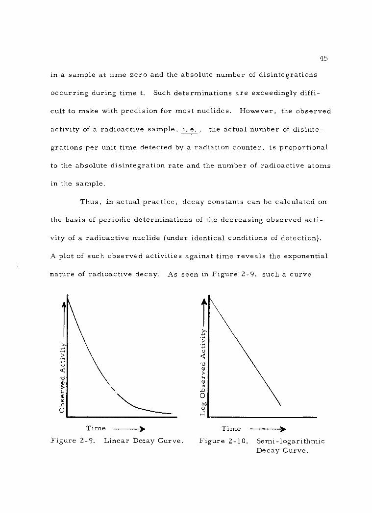
Observed Activity
45
in a sample at time zero and the absolute number of disintegrations
occurring during time t. Such determinations are exceedingly diffi-
cult to make with precision for most nuclides. However, the observed
activity of a radioactive sample, i. e. , the actual number of disinte-
grations per unit time detected by a radiation counter, is proportional
to the absolute disintegration rate and the number of radioactive atoms
in the sample.
Thus, in actual practice, decay constants can be calculated on
the basis of periodic determinations of the decreasing observed acti-
vity of a radioactive nuclide (under identical conditions of detection).
A plot of such observed activities against time reveals the exponential
nature of radioactive decay. As seen in Figure 2 -9, such a curve
Time --- Time ÷ Figure 2 -9. Linear Decay Curve. Figure 2 -10. Semi - logarithmic
Decay Curve.
1
Á o

46
flattens out and approaches zero. If the same plot is made on a semi -
logarithmic scale (Figure 2 -10), the decay curve becomes a straight
line, with a slope equal to the value of X . Krohn (5) cites practical
methods for estimating exponential decay based on a minimum number
of observations. Table 2 -2 lists decay constants for several common-
ly used radionuclides that have been thus derived.
Radioactive decay must be considered in radiotracer experi-
mental design whenever the magnitude of such decay is significant.
Table 2 -2. Decay constants for selected radioisotopes.
Nuclide Decay Constant (1. )
p32 0. 04873/day
S35 0.00794/day
Ca45 0. 00422/day
Fe55 0.00493/week
Fe59 0.01530/day
Co60 0. 01098/month
Zn65 0. 01985/week
1131 0. 00358/hour
Decay corrections may be determined directly from a prepared plot,
such as that shown in Figure 2 -10. Alternatively, corrections for
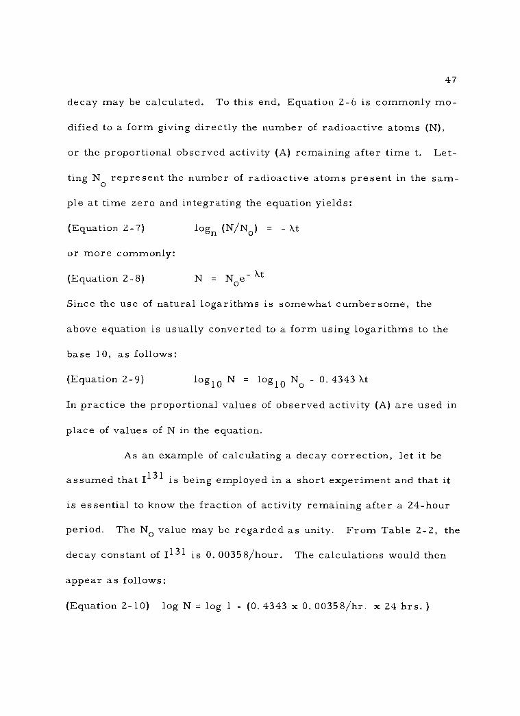
47
decay may be calculated. To this end, Equation 2 -6 is commonly mo-
dified to a form giving directly the number of radioactive atoms (N),
or the proportional observed activity (A) remaining after time t. Let-
ting No represent the number of radioactive atoms present in the sam-
ple at time zero and integrating the equation yields:
(Equation 2 -7)
or more commonly:
(Equation 2 -8)
logo (N /No) = - kt
N = Noe- At
Since the use of natural logarithms is somewhat cumbersome, the
above equation is usually converted to a form using logarithms to the
base 10, as follows:
(Equation 2 -9) log10 N = log10 No - 0. 4343 Xt
In practice the proportional values of observed activity (A) are used in
place of values of N in the equation.
As an example of calculating a decay correction, let it be
assumed that 1131 is being employed in a short experiment and that it
is essential to know the fraction of activity remaining after a 24 -hour
period. The No value may be regarded as unity. From Table 2 -2, the
decay constant of 1131 is 0. 00358 /hour. The calculations would then
appear as follows:
(Equation 2 -10) log N = log 1 - (0. 4343 x 0. 00358/hr. x 24 hrs. )
48
log N = 0 - 0. 03732 or 9. 96268 - 10
N = 0. 9177
Thus, after 24 hours, the I131 would have decayed to 91. 77 percent of
its original activity.
If an investigator expects to make extensive use of a speci-
fic radioisotope, it is often convenient to construct a decay correction
table for that isotope. A table of this type for P32 is illustrated in
Table 2 -3. It is easily prepared from the known decay constant for
the nuclide. Such tables allow rapid, yet accurate determination of
the fraction of original activity remaining in a sample after a given in-
terval of time.
2. Half -life
Another important constant, the half -life (t1), is related to
2 the decay constant. A distinctive half -life is an identifying property of
each radioactive nuclide. The half -life of a radionuclide is the time
required for its activity to decrease by one -half. Thus, after one
half -life, 50 percent of the initial activity remains. After two half -
lives, only 25 percent of the initial activity remains, and after three
half -lives, only 12.5 percent is yet present, etc. Figure 2 -11 shows
this relation graphically.

49
Table 2 -3. Decay correction table for phosphorus -32.
Hour s 0 3 6 9 12 15 18 21
Days 0 1. 0000 . 9939 . 9879 . 9819 . 9759 . 9700 . 9641 . 9582 1 . 9524 . 9466 . 9409 . 9352 . 9295 . 9238 . 9182 . 9127 2 . 9071 . 9016 . 8961 . 8907 . 8852 . 8799 . 8746 . 8692 3 . 8639 . 8587 . 8534 . 8483 . 8431 . 8380 . 8329 . 8279 4 . 8228 . 8178 . 8129 . 8079 . 8030 . 7981 . 7933 . 7885 5 . 7837 . 7789 . 7742 . 7695 . 7648 . 7602 . 7556 . 7510 6 . 7464 . 7419 . 7374 . 7329 . 7284 . 7240 . 7196 . 7152 7 . 7109 . 7066 . 7023 . 6980 . 6938 . 6896 . 6854 . 6812 8 . 6771 . 6729 . 6689 . 6648 . 6608 . 6567 . 6528 . 6488 9 . 6448 . 6409 . 6370 . 6332 . 6293 . 6255 . 6217 . 6179
10 . 6124 . 6104 . 6067 . 6030 . 5 994 . 5957 . 5921 . 5885 11 . 5849 . 5814 . 5779 . 5743 . 5709 . 5674 . 5640 . 5605 12 . 5571 . 5537 . 5504 . 5470 . 5437 . 5404 . 5371 . 5338 13 . 5306 . 5274 . 5242 . 5210 . 5178 . 5147 . 5116 . 5085 14 . 5 054 . 5023 . 4992 . 4962 . 4932 . 4902 . 4872 . 4843 15 . 4813 . 4783 . 4755 . 4726 . 4697 . 4668 . 4640 . 4612 16 . 4584 . 4556 . 4529 . 4502 . 4474 . 4447 . 4420 . 4393 17 . 4366 . 4339 . 4313 . 4287 . 4261 . 4235 . 4209 . 4183 18 . 4158 . 4133 . 4108 . 4083 . 4058 . 4033 . 4009 . 3985 19 . 3960 . 3936 . 3913 . 3889 . 3865 . 3841 . 3818 . 3795 20 . 3772 . 3749 . 3726 . 3703 . 3681 . 3659 . 3637 . 3615 21 . 3593 . 3571 . 3549 . 3527 . 3506 . 3485 . 3464 . 3443 22 . 3422 . 3401 . 3380 . 3359 . 3339 . 3319 . 3299 . 3279
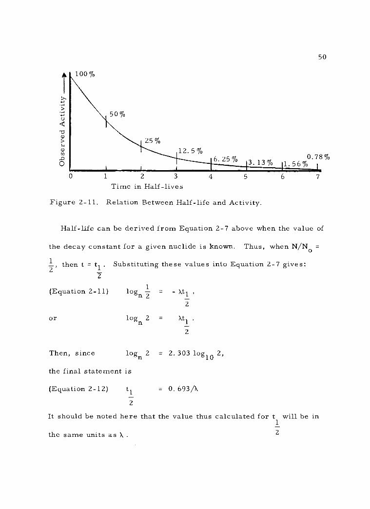
Observed
i
100%
50%
25% 12.5%
6. 25% 3.13%
2 3
Time in Half -lives
50
0.78% 1.56%
Figure 2 -11. Relation Between Half -life and Activity.
Half -life can be derived from Equation 2 -7 above when the value of
the decay constant for a given nuclide is known. Thus, when N /No =
1
2, then t=t1.
2
(Equation 2-11)
or
Substituting these values into Equation 2-7 gives :
logn 2 = - Xtl ,
2
logn 2 = Xtl
2
Then, since logn 2 = 2. 303 log10 2,
the final statement is
(Equation 2 -12) t1 = 0. 693/X
2
It should be noted here that the value thus calculated for t will be in 1
2 the same units as X..
2
0 1 4 5 6 7
51
The half -life for different nuclides ranges from under 10 -6 sec.
to 1010 years. This value has been ascertained for all the commonly
used radionuclides. When an unknown radioactive isotope is encoun-
tered, a determination of its half -life is normally the first step in its
identification. This can be done by preparing a semi -log plot of a
series of activity observations made over a period of time. A short -
lived nuclide may be observed as it decays through a complete half -
life, and the time interval observed directly (Figure 2 -12).
Acute difficulty is encountered in determining the half -life of a very
long -lived radionuclide (several hundred years or more). Here, prac-
tically no variation in disintegration rate (activity) is noticeable. In
this case, the decay constant must be accurately calculated from the
absolute decay rate according to Equation 2 -6. The absolute number
of atoms present (N) can be calculated from a precisely known weight
of a highly purified sample of the nuclide (as determined by mass
spectrometry), the atomic weight of the nuclide, and Avogadro's num-
ber (the number of atoms in a gram atomic weight of a nuclide). Thus,
(Equation 2 -13) N_ (Avogadr.,`s no,) 6.02 x 1 C;23 X a.ctua' wt. of nuclide atomic weight of. nuclide
It can then be stated that:
(Equation 2 -14) Decay Constant - dis. actually occurring /in unit time actual no. of atoms present orig.
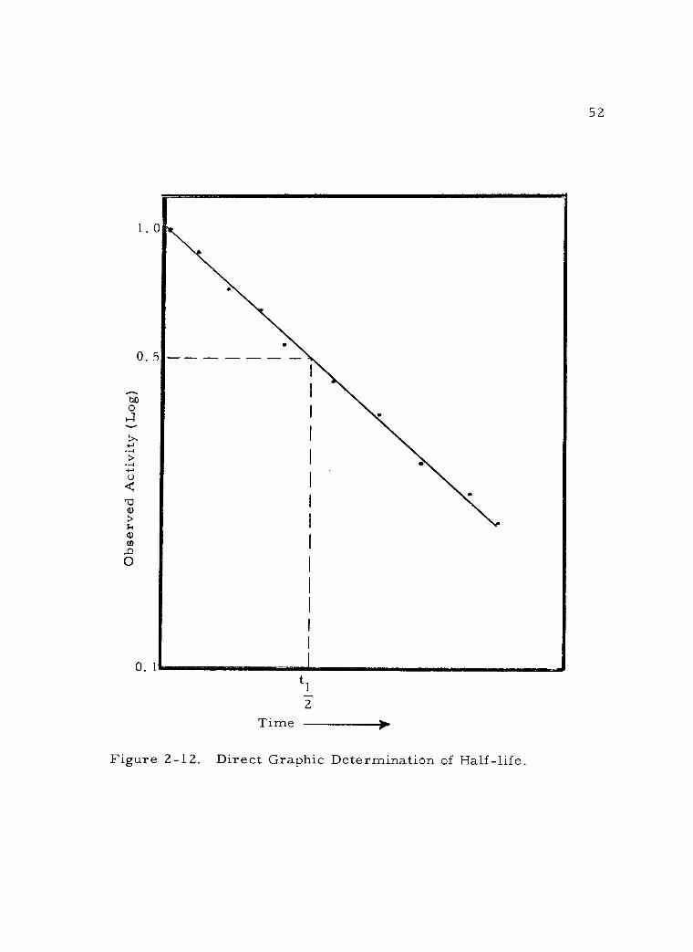
52
tl
2
Time Po
Figure 2 -12. Direct Graphic Determination of Half -life.
or in symbols:
(Equation 2 -15) X = dN/dt
No
53
When the decay constant is thus found, the half -life can be readily cal-
culated with a reasonable degree of accuracy. Conversely, Estabrook
(2) lists factors allowing ready conversion of t1 to X in any desired
time unit. 2
Highly precise determinations of half -life values are extremely
difficult to make. Variations in these values will thus be seen in pub-
lished data. The technical problems involved in such determinations
are described by Anders (1) for the short -lived nuclide P32, and by
Mann (6) in the case of the long -lived radioelement C14. The values
indicated in Table 2 -4 are average values as given by Slack and Way
(12, Chapter 1). Geiger (3) gives an extensive table of slow- neutron
capture radioisotopes arranged by half -life.
3. Practical decay considerations
Several important practical considerations arise from the fore-
going discussion of radioactive decay. In the first place, it has al-
ready been mentioned that corrections for decay must be made when
radionuclides with short half -lives are being used in tracer studies ex-
tending over a period of time.

54
Table 2 -4. Half -life values for some selected radioisotopes.
Nuclide t 1
2
Nuclide t 1
2
K42 12.42 ± 0.03 hrs. S35 87.2 ± 0. 1 days
Na24 14.97 ± 0.02 hrs. Ca45 164 ± 4 days
Y90 64.03 ± 0.05 hrs. Zn65 244.4 ± 0.5 days
Au198 2. 696 ± 0. 002 days Na22 2.58 ± 0.03 yrs.
1131 8.066 ± 0.02 days Co60 5.26 ± 0.01 yrs.
p32 14. 221 ± 0. 015 days H3 12.262 ± 0.004 yrs.
Rb86 18. 66 ± 0.02 days Sr" 28.0 ± 0.3 yrs.
Cr51 27.8 ± 0. 1 days C14 5568 t 30 yrs.
Fe59 45.3 ± 0.2 days C136 3. 03 ± 0. 03 x 105 yrs.
The second implication of radioactive decay also applies point-
edly to isotopes with short half -lives. If one experimentally adminis-
ters a high level of radioactivity to an organism, a certain amount of
radiation damage to tissues may be anticipated, depending on the rate
of elimination of the nuclide from the organism (biological half- life).
This biological effect tends to be minimized where the isotope used
decays away rapidly. Thus, with all other factors being equal, an
organism could more readily tolerate a large dose of a short lived
55
radioisotope than an equivalent dose of a longer -lived nuclide of the
same element. Where a choice of radioisotopes of the element in
question exists, as in the case of sodium (Na22 or Na24) this may be-
come an important factor in designing the experiment.
The third consideration involving rate of decay deals with the
problem of disposal of radionuclide wastes at the end of an experiment.
This will be considered in a later chapter in greater detail. However,
it will be readily seen that, particularly in the case of isotopes with
long half -lives, disposal can be a problem. Where the half -life is a
matter of a few days or weeks, and only small tracer amounts of iso-
tope are involved, it is possible to store the wastes in a restricted
area for a time equal to about 10 half -lives. The rate of decay is such
that at the end of this period the amount of activity will be reduced by a
factor of 1,000, and the wastes may be disposed of through public
channels.
4. Composite decay
Where two or more radioisotopes with different half -lives are
present in a sample, a composite decay rate will be observed. The
decay curve drawn on a semi -logarithmic plot will, in this situation,
not be a straight line. The decay curves of each of the isotopes pre-
sent may be resolved by graphic means, if their half -lives differ
56
sufficiently, and not more than three radioactive components are pre-
sent. In the graphic example shown in Figure 2 -13, line C represents
the observed activity. Only the activity of the longer -lived component
A is observed after the shorter -lived component B has decayed out.
Extrapolation of this linear portion of the curve back to zero time
gives the decay curve for component A. The curve for component B
is drawn by subtracting out point by point the activity values of com-
ponent A from the composite curve.
If the half -lives of the two components in such samples are not
sufficiently different to allow graphic resolution, the differential de-
tection method may be applicable. If the radiation characteristics of
the isotopes in the mixture are suitably distinct, it may be possible to
measure the activity of one component without interference from the
radiation emitted by the other component. A case in point would be
where one nuclide was a pure beta emitter, while the other emitted
both beta and gamma rays. Perkel (7) describes several methods for
resolving various types of complex decay curves.
Other types of composite decay occur, but are normally
not encountered in biological applications of radiotracers. Perhaps
the only such situation met with any frequency concerns "parent"
radionuclides that decay into "daughter" nuclides that are also radio-
active. In this case it is the combined activity of the parent and

1. 0 0. 9
57
Time
Figure 2 -13. Graphic Resolution of a Composite Decay Curve.
i
A
\ß (c-n)
\
58
daughter nuclides that will be observed. Two of the more common
examples of parent- daughter mixtures that the biologist may encoun-
ter are Sr90 (parent) - -- Y90 (daughter) and Cs137 (parent) - -- Ba137
(daughter). Kirby (4) describes methods of resolving such parent -
daughter mixtures mathematically.
5. Average life
While the half -life of a radionuclide composed of large num-
bers of atoms is a fixed value, the actual time to disintegration for
any individual atom can be anywhere from zero seconds to infinity.
The average length of time to disintegration for an unstable atom can,
however, be calculated. The average life (TA) is also related to the
decay constant. It is calculated as the reciprocal of the decay con-
stant:
(Equation 2-16) T = 1/X ,
A
or this can be reduced to the form:
(Equation 2-17) T = 1.443 t1 A
-2-
Average life values find primary application in the calculation of the
total number of particles emitted during complete decay. This num-
ber is used in determining total radiation dose delivered by a radio-
isotope sample, as in medical research and therapy. Table 2 -5 lists
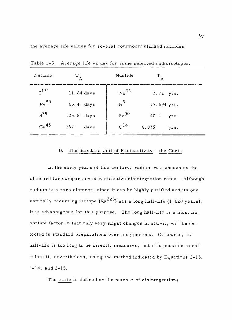
59
the average life values for several commonly utilized nuclides.
Table 2 -5. Average life values for some selected radioisotopes.
Nuclide T Nuclide T
1131
A
11. 64 days Na22
A
3. 72 yrs.
Fe59 65.4 days H3 17. 694 yrs.
S35 125.8 days Sr90 40.4 yrs.
Ca45 237 days C14 8,035 yrs.
D. The Standard Unit of Radioactivity - the Curie
In the early years of this century, radium was chosen as the
standard for comparison of radioactive disintegration rates. Although
radium is a rare element, since it can be highly purified and its one
naturally occurring isotope (Ra226) has a long half -life (1, 620 years),
it is advantageous for this purpose. The long half -life is a most im-
portant factor in that only very slight changes in activity will be de-
tected in standard preparations over long periods. Of course, its
half -life is too long to be directly measured, but it is possible to cal-
culate it, nevertheless, using the method indicated by Equations 2 -13,
2 -14, and 2 -15.
The curie is defined as the number of disintegrations

60
occurring in one gram of pure radium per second. This value has
been accurately measured many times. It may also be calculated on a
theoretical basis. Using the calculated half -life value for radium of
1590 years and substituting it into Equation 2 -12 above gives:
(Equation 2 -18) 1.59 x 10³ yrs. 0. 693
Rearranging the equation and solving for the decay constant per se-
cond shows:
(Equation 2-19) X - 0. 693
1. 59 x 103 yrs.
1 . 38 x 10-11/sec.
0. 693
5 x 10¹⁰ sec.
Since the atomic weight of radium is 226, and by Avogadro's number
there are 6. 02 x 1023 atoms in one gram atom, it can be readily cal-
culated that one gram of radium contains approximately 2. 6 x 10²¹
atoms. The decay rate of one gram of radium would be equal to the
product of the decay constant times the number of atoms in one gram,
or
(Equation 2 -20) Decay rate for 1 gm. radium /sec. =
(1.38 x 10⁻¹¹)(2.6 x 10²¹) = 3. 7 x 10¹⁰ disintegra-
tions per second (dps).
Thus, the value of the curie unit, both by calculation and definition, is
3. 7 x 10¹⁰ dps.
-
61
Since the curie is a relatively large unit, several subdivisions of
it are in common use. These are the millicurie (mc), which is equal
to 1/1,000 of a curie, or 3. 7 x 10⁷ dps, and the microcurie (tic),
which is 1/1,000,000 of a curie, or 37, 000 dps, or 2. 2 x 10⁶ disinte-
grations per minute (dpm).
It should be noted that the curie unit refers to the actual number
of disintegrations occurring in a sample, rather than the disintegra-
tions detected by a radiation counter. The difficulties of actually de-
tecting the absolute number of disintegrations occurring in a sample
will be pointed out in a later chapter. The disintegration rate detected
by a counting assembly is normally only a fraction of the absolute dis-
integration rate of the sample.
It should also be emphasized that the curie is based on the rate
of nuclear disintegration, not the rate of emission of beta particles,
gamma rays, or other radiation. To calculate such emission rates
requires reference to the decay scheme of the nuclide. For example,
gold -198 usually emits a beta particle and one gamma ray for each
nuclear disintegration, while cobalt -60 commonly emits a beta parti-
cle and two gamma rays of different energies per nuclear disintegra-
tion. Thus, for the same curie level of these two isotopes, the Co66
would emit twice the number of gamma photons as the Au' 98. This
problem is further complicated where a nuclide has alternate paths of
62
decay. Consideration of this factor is important in connection with
the calculation of disintegration rate from the counting rate as meas-
ured by a detecting instrument, and in radiation dose calculations.
E. Specific Activity
In isolating the products of reactor or cyclotron irradiation, it
is usually possible to achieve chemical separation of nuclides of the
element sought from other elements in the sample. It is a different
matter, however, to completely separate a specific nuclide from other
nuclides of the same element in the sample material, since all of the
isotopes of a given element are chemically identical. These other
nuclides may have been originally present in the sample, or produced
in it by competing nuclear reactions during irradiation. The problem
of separation is particularly acute for radionuclides produced by the
(n, y) process in reactors, for here the parent material and the pro-
duct are isotopes of the same element. Thus, depending on the speci-
fic method of production employed and the degree of separation pos-
sible, processed radionuclide samples will contain varying amounts of
other isotopic material of the same element.
The ratio that exists between the atoms of a given radioactive
isotope and the total number of atoms of the same element present in
a sample is known as the specific activity of the sample. Specific
63
activity is usually expressed in terms of the disintegration rate in
curies (or mc, µc or dpm) of the specific radionuclide per unit mass
of the element. Very high specific activities are obtainable for cer-
tain radioisotopes. Tritium gas, as an extreme example, can be se-
cured with a specific activity of 2. 59 curies per cc at STP. The term
carrier free is sometimes applied to samples of such high specific
activity that essentially all the atoms of the element in question are of
the same radioactive species.
In the design of radiotracer experiments (see Chapter 10) it is
essential to calculate the specific activity of the tracer required. Use
of a very low specific activity may result in counting samples with too
low an activity level to be detected. In general, it is advisable to uti-
lize a fairly high specific activity initially to allow for the dilution fac-
tor inherent in most biological radiotracer experiments. Unfortu-
nately, for a given nuclide it is generally true that the higher the spe-
cific activity of the sample material, the greater the expense of pro-
ducing it. This unpleasant economic relationship is illustrated in
Table 2 -6, based on current prices from the Oak Ridge National
Laboratory (see Chapter 11). Experimental design must usually in-
clude consideration of this economic factor.
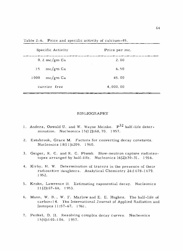
64
Table 2 -6. Price and specific activity of calcium -45.
Specific Activity Price per mc.
0. 2 mc/gm Ca
15 me /gm Ca
1000 mc/gm Ca
carrier free
2. 00
6. 50
45. 00
4, 000. 00
BIBLIOGRAPHY
1. Anders, Oswald U. and W. Wayne Meinke. P32 half -life deter- mination. Nucleonics 15(1 2):68, 70. 1957.
2. Estabrook, Grace M. Factors for converting decay constants. Nucleonics 1 8(11 ):209. 1 960.
3. Geiger, R. C. and R. C. Plumb. Slow- neutron capture radioiso- topes arranged by half -life. Nucleonics 14(2):30 -31. 1956.
4. Kirby, H. W. Determination of tracers in the presence of their radioactive daughters. Analytical Chemistry 24:1 678 -1679. 1 95 2.
5. Krohn, Lawrence H. Estimating exponential decay. Nucleonics 11(2):67-68. 1953.
6. Mann, W. B. , W. F. Marlow and E. E. Hughes. The half -life of carbon -14. The International Journal of Applied Radiation and Isotopes 1 1 :57- 67. 1 961 .
7. Perkel, D. H. Resolving complex decay curves. Nucleonics 1 5(6):1 06. 1957.
65
CHAPTER 3 - CHARACTERISTICS OF IONIZING RADIATION
It has been seen that nuclear radiation occurs as a result of
spontaneous disintegrations of atomic nuclei. These nuclear changes
can give rise to several types of radiation, of which the following
have already been indicated: (1) alpha particles; (2) negative beta
particles, or negatrons; (3) positive beta particles, or positrons;
(4) x -rays resulting from electron capture; (5) gamma rays; either
from isomeric transition or, more commonly, as excess energy fol-
lowing particle emission; (6) internal conversion electrons, resulting
from gamma ray interaction with orbital electrons.
The radiation types most commonly detected from isotopes
used as radiotracers are alpha particles, beta particles (either posi-
tive or negative), and gamma rays. These radiation types differ radi-
cally in their physical characteristics. Alpha radiation is made up
of rather massive particles (helium nuclei) with a doubly positive
charge that move at a relatively slow velocity (only a small fraction
of the speed of light). By contrast, beta radiation consists of singly
charged particles of extremely small mass, which are emitted with
velocities approaching the speed of light. Gamma rays are electro-
magnetic radiation (photons), which are uncharged and travel at the
speed of light. The characteristics of these three types of radiation
will be more extensively discussed in this chapter.
A. Alpha Particles
1. Energy
66
Alpha emitting isotopes are not commonly used as tracers in
biological investigations. This is due in large part to the fact that
most alpha emitting nuclides are elements of high atomic number (Z
above 82), which are not normally metabolically significant in living
plants and animals. Their presence in the environment, however,
constitutes a considerable biological hazard and they are studied by
the biologist primarily from this standpoint.
The alpha particle has been previously described as a helium
nucleus composed of two neutrons and two protons - -- a rather mas-
sive particle. Due to this large mass and the doubly positive charge
the alpha particle exerts a considerable electrostatic attraction on
the outer orbital electrons of the atoms near which it passes. In ad-
dition, alpha particles tend to follow very straight paths. Normally,
only a rare direct collision with a nucleus causes them to be deflec-
ted.
Alpha particles are emitted from unstable nuclei with consi-
derable kinetic energy. The range of energy from natural alpha
67
emitting sources lies between about four to eight Mev. Probably the
most significant feature of alpha particle energy is that it is discrete,
that is, all the alpha particles emitted by a specific nuclide will
emerge at one or a few defined energy levels. As examples, Ra221
emits all of its alpha particles at an energy of 6. 71 Mev, while U23°
emits alpha particles with energy levels of 5. 89 Mev, 5. 82 Mev, or
5. 66 Mev. Such discrete energy levels of alpha emission serve as a
means of identifying specific nuclides.
2. Half -life and energy
It was noted quite early that the half -life of a specific nuclide
generally seemed inversely related to the alpha particle energy of
that nuclide. The current concept of the mechanism of alpha particle
emission provides an explanation of this relationship. According to
this concept, the dense concentration of positively charged protons in
the nucleus of an atom of high atomic weight produces an extremely
strong potential barrier immediately around the nucleus. This poten-
tial barrier acts to repel charged particles approaching the nucleus.
Moreover, the barrier serves to entrap the nucleons within it in an
"energy well ", preventing their escape in the form of an alpha parti-
cle. The term "barrier" is used only in a figurative sense to repre-
sent a repulsive force field.

68
Figure 3 -1 is a graphic representation of a cross section
through this barrier and the nuclear energy well. The stippled area
denotes excess energy in the nucleus which may be imparted to an
alpha particle when the nucleus undergoes alpha decay. Such an
event will reduce the energy level of the nucleus to a more stable
level. Because this excess energy in the nucleus is much lower than
the energy of the potential barrier, an alpha particle, as such, can-
not escape from the nucleus. However, according to the principles
of wave mechanics, a finite probability exists that the alpha particle
may "tunnel" through the barrier in the form of a wave and emerge
as a particle which is then actively repelled. The probability of such
an occurrence is inversely related to the magnitude of the potential
barrier to be penetrated, as depicted in Figure 3-1. Therefore, the
higher the excess energy level within the "energy well, " the less the
potential barrier to be penetrated and, thus, the greater the probabi-
lity of alpha particle escape. A higher rate of escape will, of course,
be related to a shorter half -life for a given nuclide. On the other
hand, where the alpha energy is relatively low, the probability of
escape is small, and the half -life is longer. This same general con-
cept, with modifications, is also involved in beta and gamma radia-
tion from the nucleus.
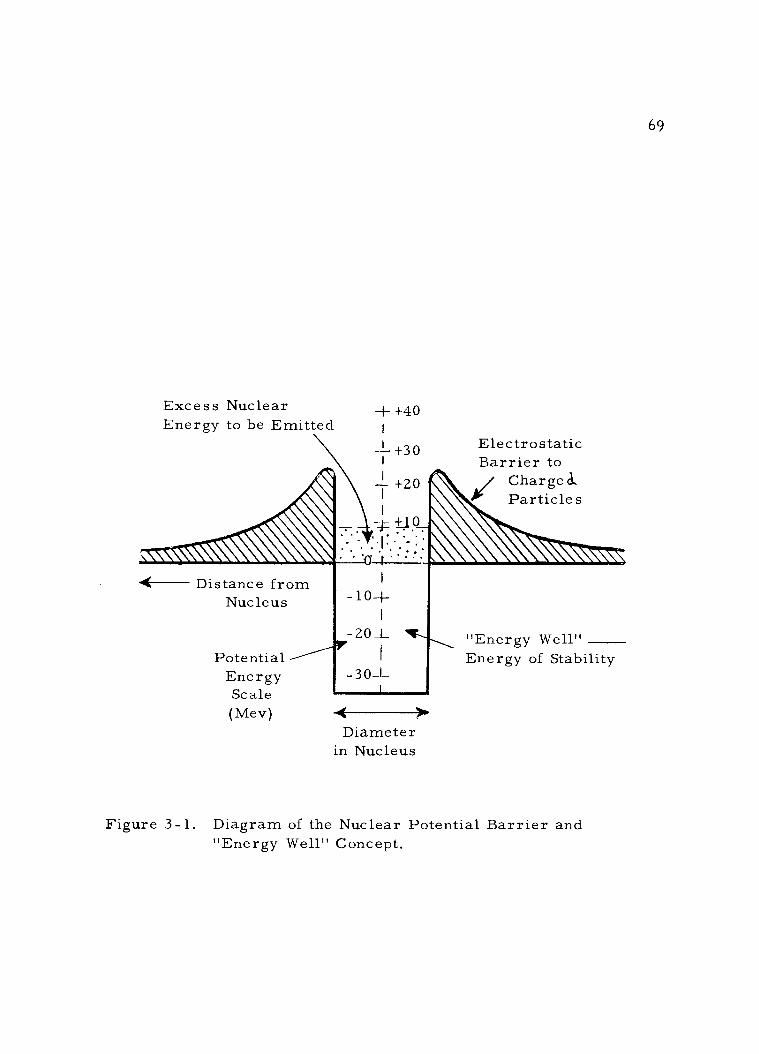
69
Excess Nuclear --I- +40 Energy to be Emitted
I +30
TI +20
Distance from Nucleus
Potential Energy Scale (Mev)
Electrostatic Barrier to
Charged. Particles
-30 -L
Diameter in Nucleus
"Energy Well" Energy of Stability
Figure 3-1. Diagram of the Nuclear Potential Barrier and "Energy Well" Concept.
i
-10-4--
-20_L
1
I
1
i
'N
f-
( T
/ i

70
3. Interaction with matter
The strong electrostatic field surrounding a doubly charged
alpha particle exerts a considerable attraction for the orbital elec-
trons of the atoms near its path. In many cases electrons in the
outermost orbits may be stripped completely away from their atoms.
In other cases, electrons in inner orbits may be drawn out to orbits
further from their nuclei. Such interactions with orbital electrons
dissipate the kinetic energy of the alpha particle.
a. Excitation: The term excitation is used to describe inter-
action whereby orbital electrons take up energy, but are not removed
completely from their atoms. After the passage of the alpha particle,
the excited electrons fall back into their former orbits and emit their
excess energy as a photon. Detection of such light flashes, as will be
seen in Chapter 5, is the basis of scintillation counting.
b. Ionization: The first type of interaction mentioned above,
where the alpha field strips orbital electrons from their atoms, is
known as ionization. The loss of a negatively charged electron leaves
the atom as a positively charged ion. The electron and the positive
atom are together known as an ion pair. The formation of each ion
pair in air requires on the average about 35 electron volts of the
alpha particle's kinetic energy. Stated another way, a 7. 0 Mev alpha
71
particle will produce about 2 x 10⁵ ion pairs in air before its energy
is completely dissipated. The effect of ionization can be visualized
in a cloud chamber, where each ion produced serves as a nucleus for
the formation of a fog droplet in a supersaturated atmosphere. An
alpha track in a cloud chamber appears as a straight, dense fog trail,
made up of thousands of droplets per centimeter.
c. Specific ionization: For a quantitative description of the
ionization occurring along the alpha track, the term specific ioniza-
tion is used. Specific ionization is the number of ion pairs formed
per unit length (cm) of the alpha particle's path in air at standard
pressure. Figure 3 -2 shows the variation in specific ionization for
alpha particles over the extent of their range in the air. It is clearly
evident that the specific ionization of a beam of alpha particles in-
creases sharply toward the end of their range. This is so because,
as a result of many collisions with gas atoms, the alpha particles
have lost much kinetic energy and their velocity has decreased. Due
to this reduced velocity, they remain in the vicinity of atoms along
their path for a longer period of time and, thus, have a much greater
probability of interacting with these atoms. After specific ionization
reaches a peak, it drops sharply to zero. At this point, the alpha
particles have expended their kinetic energy, picked up two electrons,
and become neutral helium -4 atoms.

Specific
Ionization
0 Range in Air -)
72
Figure 3 -2. Typical Specific Ionization Curve for Alpha Particles in Air.
Alpha
1. 0
Intensity 0 5
Distance from Source in Air
Mean Range
Extrapolated Range
Figure 3 -3. Typical Range Curve for Alpha Particles in Air.
4. Range
73
a. Determination: Because of the discrete energy of alpha
emission, alpha particles from a given radioactive source will have a
clearly defined range. Alpha range can be experimentally determined
by measuring the intensity of alpha radiation at increasing distances
from an alpha emitter. Figure 3 -3 represents a plot of such data. It
will be seen that the number of alpha particles detected remains con-
stant for a considerable distance from the emitting source. Finally
the radiation intensity detected drops sharply to zero.
The mean range is the distance from the source at which the
initial alpha radiation intensity is reduced to one half. This mean
range is usually only a few millimeters in air less than the extrapo-
lated range and is much more accurately determined. A certain
amount of straggling of the alpha particles produces the tail on the
range curve in Figure 3 -3. This makes absolute determination of the
true range difficult.
b. Range- energy relations: The range of alpha particles is,
of course, directly related to the kinetic energy with which they are
emitted. Unfortunately, this is not a simple relationship. The use of
Equation 3 -1 allows the calculation of an approximate range for alpha
particles with energies between four to seven Mev.
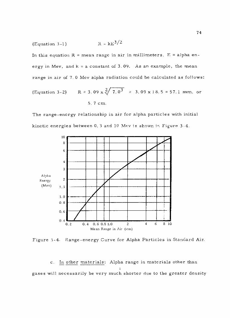
(Equation 3 -1) R = kE3/2
74
In this equation R = mean range in air in millimeters, E = alpha en-
ergy in Mev, and k = a constant of 3. 09. As an example, the mean
range in air of 7. 0 Mev alpha radiation could be calculated as follows:
(Equation 3 -2) R = 3. 09 x 7. 03 = 3. 09 x 18. 5 = 57.1 mm. or
5. 7 cm.
The range- energy relationship in air for alpha particles with initial
kinetic energies between 0. 3 and 10 Mev is shown in Figure 3 -4,
Alpha Energy (Mev)
10
8
6
4
3
2
1.5
1.0
0.8
0. 6
0. 4 0.2 0.4 0.6 0.8 1.0 2
Mean Range in Air (cm) 6 8 10
Figure 3 -4. Range- energy Curve for Alpha Particles in Standard Air.
c. In other materials: Alpha range in materials other than
gases will necessarily be very much shorter due to the greater density
4
- , 2 /
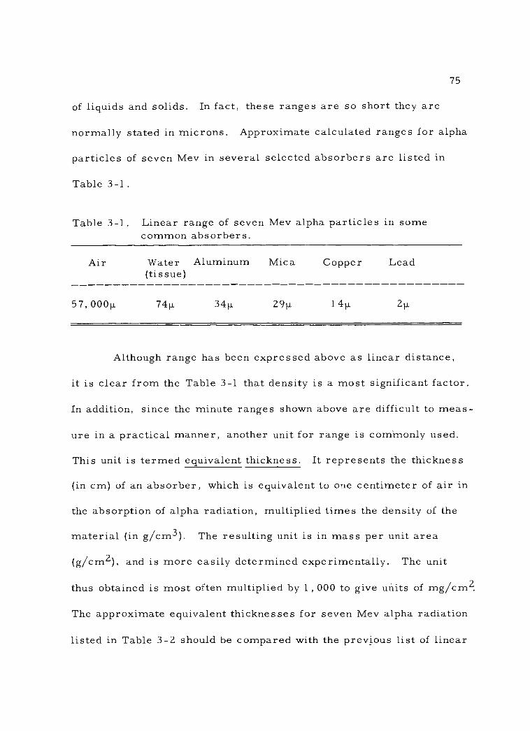
75
of liquids and solids. In fact, these ranges are so short they are
normally stated in microns. Approximate calculated ranges for alpha
particles of seven Mev in several selected absorbers are listed in
Table 3 -1.
Table 3 -1. Linear range of seven Mev alpha particles in some common absorbers.
Air Water Aluminum Mica Copper Lead (tissue)
57,00011 74µ 34µ 291.1 l411 2µ
Although range has been expressed above as linear distance,
it is clear from the Table 3 -1 that density is a most significant factor.
In addition, since the minute ranges shown above are difficult to meas-
ure in a practical manner, another unit for range is commonly used.
This unit is termed equivalent thickness. It represents the thickness
(in cm) of an absorber, which is equivalent to one centimeter of air in
the absorption of alpha radiation, multiplied times the density of the
material (in g /cm3). The resulting unit is in mass per unit area
(g /cm2), and is more easily determined experimentally. The unit
thus obtained is most often multiplied by 1 , 000 to give units of mg /cm?
The approximate equivalent thicknesses for seven Mev alpha radiation
listed in Table 3 -2 should be compared with the previous list of linear
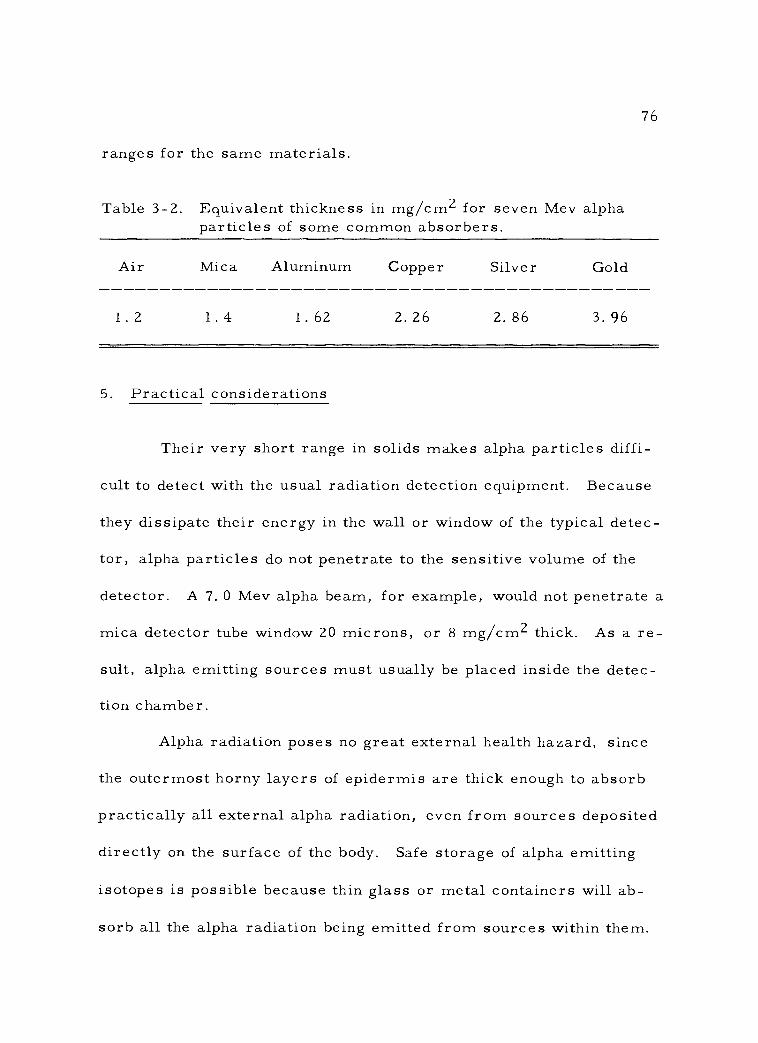
76
ranges for the same materials.
Table 3 -2. Equivalent thickness in mg /cm2 for seven Mev alpha particles of some common absorbers.
Air Mica Aluminum Copper Silver Gold
1.2 1.4 1.62 2. 26 2. 86 3. 96
5. Practical considerations
Their very short range in solids makes alpha particles diffi-
cult to detect with the usual radiation detection equipment. Because
they dissipate their energy in the wall or window of the typical detec-
tor, alpha particles do not penetrate to the sensitive volume of the
detector. A 7. 0 Mev alpha beam, for example, would not penetrate a
mica detector tube window 20 microns, or 8 mg /cm2 thick. As a re-
sult, alpha emitting sources must usually be placed inside the detec-
tion chamber.
Alpha radiation poses no great external health hazard, since
the outermost horny layers of epidermis are thick enough to absorb
practically all external alpha radiation, even from sources deposited
directly on the surface of the body. Safe storage of alpha emitting
isotopes is possible because thin glass or metal containers will ab-
sorb all the alpha radiation being emitted from sources within them.
77
When alpha emitters enter the body by ingestion or inhalation
the situation is quite different. Alpha particles dissipate their energy
in such an exceedingly small volume of tissue that very great local
damage can occur. Moreover many natural alpha emitters have long
half -lives and some (radium and plutonium) are incorporated into
metabolically less active bone tissue, thus increasing the internal
hazard. One alpha emitting nuclide of considerable prominence,
Pu239, is highly toxic from a purely chemical standpoint, in addition
to its radiation hazard.
1. General nature
B. Beta Particles
a. Negatrons and positrons: The term beta particle has been
used for two different entities - -- positrons and negatrons. These
both represent particles formed by nuclear changes and ejected from
the nucleus with velocities approaching the speed of light. They are
physically alike in nearly every respect except charge. Positrons
carry a positive charge, while negatrons are negatively charged,
i. e. , electrons.
Beta particles are only 1/7,400 the mass of alpha particles.
Due to this very small mass, they are quite easily deflected on pas-
sing near other atoms. Their track in a cloud chamber is a very

78
tortuous one indeed, wholly unlike the straight alpha track. In addi-
tion, the smaller mass and higher velocity of the beta particle results
in a smaller probability of interaction with the orbital electrons of the
atoms it passes near. Thus, it has a much longer range through mat-
ter. Where the range in air of alpha particles may be only several
centimeters, the range of beta particles may be several meters.
Since in all respects but origin, the negatron is like a normal
orbital electron, it will persist after dissipating all its kinetic energy.
Its ultimate fate is usually to become attached to a positive ion as an
orbital electron. A positron, on the other hand, has only a transient
existence. After expending all its kinetic energy it interacts with an
electron and is "annihilated ". The mass of both particles is converted
to energy in the form of two 0. 51 Mev gamma rays which are emitted
at angles of 180° to each other ( "back -to -back gamma radiation ").
Hereafter, following common practice, the term beta particle will be
used for the negatrori.
b. Conversion electrons: A similar, yet distinct, type of high
velocity radiation particle is the internal conversion electron. This
particle results when a gamma ray emitted from a disintegrating nu-
cleus interacts with an inner orbital electron of the same atom. All
of the gamma energy is imparted to this electron, ejecting it at high
speed. Since gamma rays, like alpha particles, are emitted with a
79
discrete energy, internal conversion electrons are ejected with dis-
crete energies from a given nuclide - -- in contrast to beta particle
emission. Thus, the term beta particle is restricted to electrons
originating in the nucleus. Internal conversion is not of great impor-
tance in the detection of radionuclides commonly used as biological
tracers.
Z. Energy of beta decay
a. Spectral distribution of energy: Perhaps the most unique
character of beta radiation is the particle energy. It has been seen
that a given nuclide may eject alpha particles at one or a few discrete
energy levels. By contrast, in beta decay the particles are emitted
over a continuous range of kinetic energy up to a maximum value
(Ems) characteristic of the nuclide in question. Values for beta
Emax range from 0. 01 8 Mev for H3 up to 4. 81 Mev for C138.
The magnetic spectrometer has been used experimentally to
determine the beta energy distribution for many nuclides. In this in-
strument, a collimated beam of beta particles is deflected through
1 80° by a strong magnetic field. The more energetic particles in the
beam swing in a wider arc, while the less energetic travel over a
shorter arc. As a result, the beam particles of various energies are
spread out to form a spectrum, which is detected by exposure of a
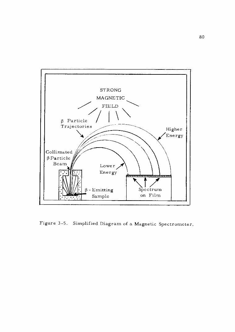
80
Particle Trajectories
Collimated ß Particle
Beam
STRONG
MAGNETIC
FIELD , Higher y z77- /Energy
Lower, Energy
p - Emitting Sample
Spectrum on Film
Figure 3 -5. Simplified Diagram of a Magnetic Spectrometer.
/ / R

81
strip of photographic film (Figure 3 -5). Alternatively, a beta- sensi-
tive detector may be placed in fixed position, instead of the film, and
the magnetic field varied so that successive energy levels of the beta
spectrum are detected. The energy of the various beta particles can
be calculated from the known strength of the magnetic field and the
radius of the arc followed by the particles. Brownell (2) discusses
this technique at greater length.
The plot shown in Figure 3 -6 of the number of beta particles
from phosphorus -32 detected at various energy levels represents a
/ E = 0. 70 Mev mean
0.5 1.0 p Particle Energy (Mev)
Emax = 1. 710 Mev
1. 5
Figure 3 -6. Energy Distribution Curve of Beta Particles from P32.
a typical beta spectrum. It will be noted that the fraction of beta
particles emitted with the maximum energy (E ) is very small. A max much larger fraction, often the largest, is emitted with the mean
energy (Emean). The value of Emean is roughly 0. 3 Emax for most
beta emitters. The range of beta particles quite obviously depends on
1 z t

82
the value of E max , but in calculating the actual radiation dose from a
beta emitter, the Emean value is used.
The energy spectra for several nuclides commonly used as
radiotracers are given in Figure 3 -7. It should be noted that the gen-
eral shape of the curves varies from nuclide to nuclide. The low
energy (soft) emitters have particularly noteworthy spectra. A dashed
line at the low energy portion of each spectrum indicates that this
portion is theoretically calculated, since experimental determination
is not readily feasible. Marshall (8) presents methods for calculating
the shape of beta spectra.
b. The neutrino and beta decay: Since discrete energy levels
were known to exist within the nucleus (see discussion above of alpha
emission energy), the emission of beta particles over a continuous
energy spectrum from the same nuclide was somewhat of an enigma.
In 1 931, to explain this, Pauli suggested that each event of beta decay
actually occurred with the emission of the maximum energy. He
postulated that a hitherto undiscovered particle, the neutrino, shares
this discrete energy with the beta particle in varying proportions from
disintegration to disintegration. For example, with P32, a beta par-
ticle with an energy of one Mev would be accompanied by a neutrino
with 0. 71 Mev energy, making a total energy emission of 1. 71 Mev.
Pauli indicated that the neutrino had no charge and negligible
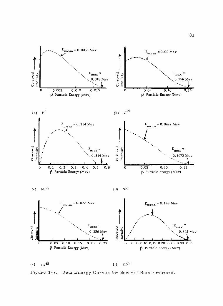
Emean = 0. 0055 Mev
H3
0.005 0.010 0.015 3 Particle Energy (Mev)
83
E = 0.05 Mev mean -- d
, . Em Emax- - n 0. 156 Mev a) Y ii
(b) C14
0.05 0. 10 0. 15
3 Particle Energy (Mev)
E = O. 214 Mev E = O. 0492 Mev mean mean l, Ì
--..
`'
71 / \ \ > / \max =
> \ Emax Ñ / 0. 544 Mev Ñ v ! 0. 1673 Mev
/ .n O \ O A
.4
0 0. 1 0. 2 0. 3 0.4 0.5 0.6 3 Particle Energy (Mev)
(c) Na22
E = 0.077 Mev mean
E - max - \256 Mev
0 0.05 0.10 0.15 0.20 0.25
(e) Ca45
0 0.05 0. 10 0. 15
Í3 Particle Energy (Mev)
( d) S35
Emean = 0. 143 Mev
Em max \ 0. 325 Mev
0.05 0.10 0.15 0.20 0.25 0.30 0.35 ¡3 Particle Energy (Mev)
Ï3 Particle Energy (Mev)
(f) Zn65
Figure 3 -7. Beta Energy Curves for Several Beta Emitters.
Emax =
0.018 Mev
0
ru \ ti
0 0
(a)
`` \ ..
v \ v
v \., \ ai ó
-11-
..
0
84
mass; as a result, its interaction with matter would be virtually nil
and its detection most unlikely. This elusive neutrino long defied de-
tection, but its existence was finally demonstrated by means of an
elaborate experimental technique in 1956. The current concept of beta
decay now stands as follows:
energy = Emax
Neutron > Proton + Beta particle + Neutrino
c. The Fermi theory of beta decay: It will be recalled that,
for alpha emitters, an inverse relation exists between alpha emission
energy and nuclide half -life. In general, such a relation also exists
for beta emitters. However, all beta emitting nuclides cannot be
grouped into a single category in this respect.
In 1934, Enrico Fermi formulated a theory of beta decay which
grouped the various emitters in a number of transition types, depend-
ing on the specific nature of the nuclear change taking place. Over a
dozen such types, in each of which the above inverse relationship
holds true, have been identified. Comparisons cannot, however, be
made between different transition types. For example, P32 and C14
are in the same transition type. The former has a half -life of 14. 2
days and an Emax of 1. 71 Mev, while the latter has a half -life of
5, 568 years and an Emax of 0. 1 56 Mev.
Fermi's general equation may be stated as follows:

(Equation 3 -3) X (decay constant) = kEmax5
85
The values of the constant k vary with the transition type. Fermi's
theory also serves to explain the varying shapes for different beta
spectra (see Figure 3 -7).
3. Interaction with matter
a. Modes of interaction: As with alpha radiation, beta parti-
cles dissipate their energy largely by ionization and excitation of the
atoms with which they interact. A third type of energy loss also oc-
curs. A high energy beta particle closely approaching the potential
barrier around a nucleus is accelerated and deflected by the encounter.
As a result, energy is lost as electromagnetic radiation. This loss of
energy results in a slowing down of the beta particle and, hence, this
type of x- radiation is commonly called Bremsstrahlung (German for
"braking radiation "). This phenomenon occurs principally when high
energy beta radiation interacts with elements of high Z. Bremsstrah-
lung is of no particular value in detecting beta radiation. On the con-
trary, it introduces serious problems in beta range determinations.
b. Specific ionization: As previously mentioned, the track of a
beta particle as seen in a cloud chamber is tortuous, poorly defined,
and much longer than that of an alpha particle. In considering an

86
initially unidirectional beam of beta radiation, it is evident that many
of the beta particles will be deflected and scattered out of the beam.
This will lead to an apparent decrease in intensity of the radiation not
due strictly to absorption. Moreover, any given beta particle may
lose a large fraction of its kinetic energy in a single collision and,
since this beam would contain beta particles with a spectrum of ener-
gies, the range of individual particles in the beam is continually vari-
able. This is quite in contrast to the situation with a beam of alpha
particles.
In view of the foregoing considerations it should be evident
that a specific ionization curve as shown for alpha radiation (Figure
3 -2) cannot be drawn for beta particles. Instead, specific ionization
must be plotted as a function of beta particle energy, since the range
of individual beta particles is so indeterminate.
It will be seen from Figure 3 -8 that specific ionization in-
creases sharply as beta energies fall below about 700 Key. The maxi-
mum specific ionization, 7, 700 ion pairs per cm, occurs at 146 ev.
Thus, the preponderance of ionization and energy loss occurs toward
the end of the beta track at energy levels below a few thousand ev. At
beta energies above about two Mev, relativistic considerations lead to
a gradually increasing specific ionization with increasing particle
energy.

87
It will be noted by comparing Figures 3 -2 and 3 -8 that specific
ionization for alpha particles is many times greater than that for beta
particles. This is understandable, since specific ionization is in-
versely related to particle velocity, and for a given kinetic energy the
velocity of a beta particle is much higher than that of an alpha particle.
o . 7-1
E ._,
o H U
w, ra
a N p, o
U]
300
250
200
150
100
50
0
\
10 -2 10- 1 10 Beta Energy (Mev)
100
Figure 3 -8. Specific Ionization Curve for Beta Particles in Air
4. Range
While the range of alpha radiation is rather clear cut, beta
range both in air and in metal absorbers is quite ill defined. Since
linear beta range in air is extremely difficult to determine experimen-
tally, range is usually expressed in equivalent thickness (in mg /cm2)
of an absorber. Aluminum is the most commonly used absorber for
,
<4
N U
"--
U r,
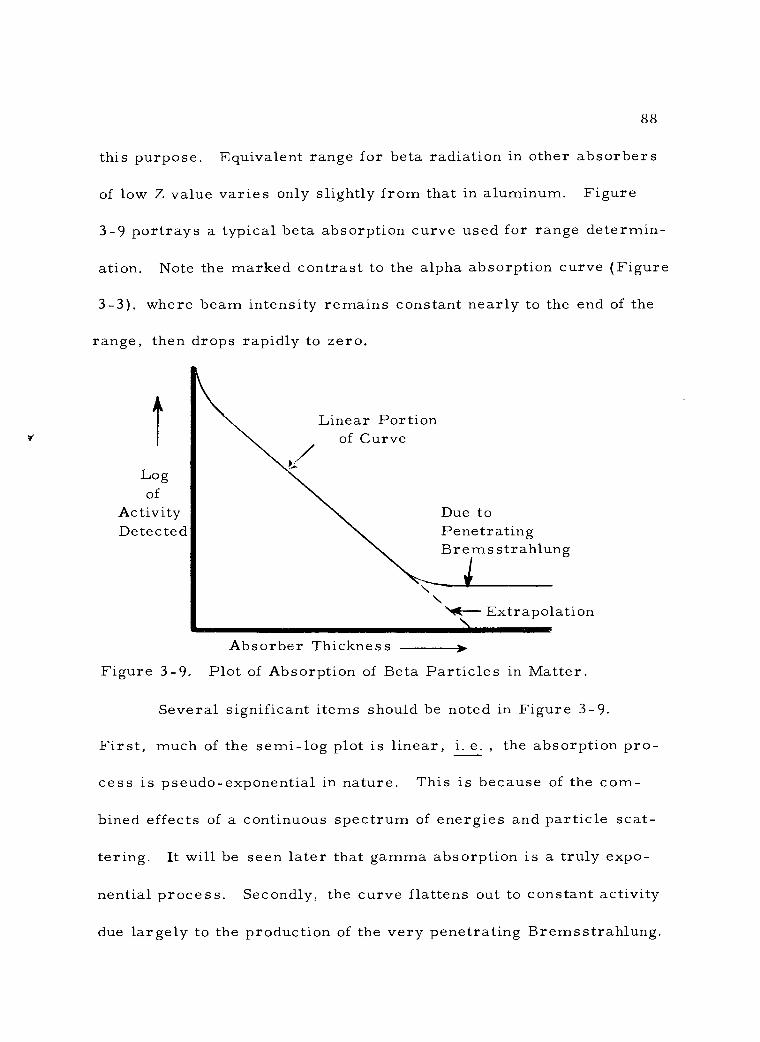
88
this purpose. Equivalent range for beta radiation in other absorbers
of low Z value varies only slightly from that in aluminum. Figure
3 -9 portrays a typical beta absorption curve used for range determin-
ation. Note the marked contrast to the alpha absorption curve (Figure
3 -3), where beam intensity remains constant nearly to the end of the
range, then drops rapidly to zero.
Log of
Activity Due to Detected Penetrating
Bremsstrahlung
Linear Portion of Curve
`tic--- Extrapolation
Absorber Thickness Figure 3 -9. Plot of Absorption of Beta Particles in Matter.
Several significant items should be noted in Figure 3 -9.
First, much of the semi -log plot is linear, i. e. , the absorption pro-
cess is pseudo - exponential in nature. This is because of the corn -
bined effects of a continuous spectrum of energies and particle scat-
tering. It will be seen later that gamma absorption is a truly expo-
nential process. Secondly, the curve flattens out to constant activity
due largely to the production of the very penetrating Bremsstrahlung.
89
Thirdly, although it would seem that extrapolation of the linear por-
tion of the curve would give the true beta range, this is unfortunately
not the case.
Accurate experimental determination of the maximum range
(Rm ) is important as a basis for calculating Emax. Since the Emax
value is a distinctive characteristic of each nuclide, its determination
is most important in identifying the presence of a specific beta emit-
ter in an unknown sample. The Feather analysis is one of the most
commonly used methods to derive Rmax from an absorption curve.
This method involves comparison of the absorption curve in aluminum
of an unknown beta emitter with that of a beta emitter having a known
range. Further discussion of beta range- energy relations will be
found in Katz (7), Barreira (1), and Duncan (3).
5. Practical considerations
a. In detection: In the application of radioisotopes as tracers,
the identity of the nuclide being used is normally known. Thus, it is
not necessary to determine experimentally the R max and E max of the
nuclide in question. Instead, the concern of the investigator centers
on the limitations on detection imposed by beta particle range and
energy. Since the detection of beta radiation commonly necessitates
the particles entering an enclosed chamber through a "window, " it is
max
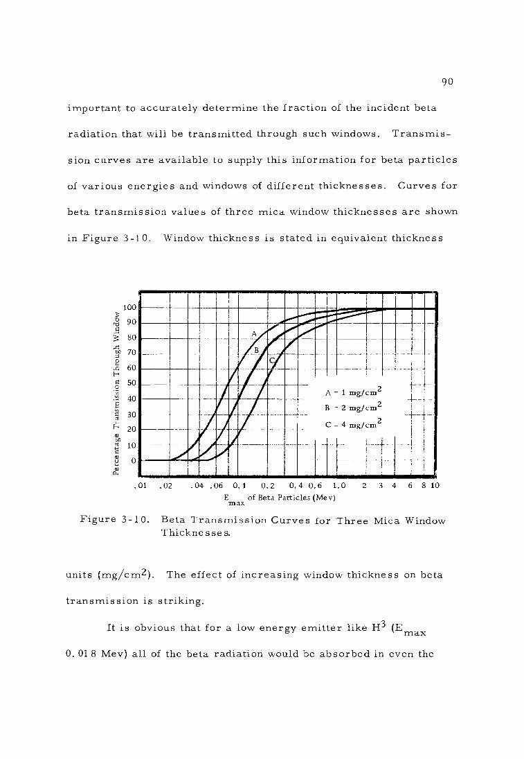
e T
rans
mis
sion
Tho
ugh
Win
dom
90
important to accurately determine the fraction of the incident beta
radiation that will be transmitted through such windows. Transmis-
sion curves are available to supply this information for beta particles
of various energies and windows of different thicknesses. Curves for
beta transmission values of three mica window thicknesses are shown
in Figure 3 -10. Window thickness is stated in equivalent thickness
100
o 90 v a
80
bo 70 o
Ñ 60
ó 50
40
ro 30
20 v 00
. .
PA /. ------- - "--
.. -f
- .. _
-
---- -- --_.. "------ - ------
A =
B -
C=4mg/cm2
_
1 mg/cm2
2 mg/cm2 ,1 I
ill
. -{- +
,_ /Oprf i
.01 .02 .04 .06 0.1 02 0.4 0 6 1.0 E of Beta Particles (Mev)
2 3 4 6 8 10
Figure 3 -10. Beta Transmission Curves for Three Mica Window Thickne s se s.
units (mg /cm2). The effect of increasing window thickness on beta
transmission is striking.
It is obvious that for a low energy emitter like H3 (Emax
0. 01 8 Mev) all of the beta radiation would be absorbed in even the
E
;; 10
ti 0
á
.!...á _ n
I
-- -- ,
._. .-- I -1--±
-'r--fi
. --
max
_ ..
f

91
thinnest window shown in Figure 3 -10. Unfortunately, several other
isotopes of biological importance, such as C14 (Emax 0. 0.156 Mev),
S35 (Emax 0.1 673 Mev), and Ca45 (Emax O. 256 Mev), also emit very
"soft" beta radiation. Much, if not all, of the radiation from these
isotopes would be absorbed before actually entering the sensitive vol-
ume of a gas filled ionization type detector. It is therefore necessary
to use special detecting techniques for these soft emitters. These
techniques, which will be further described in Chapter 4, customarily
involve using an ultrathin window detector, placing the radioactive
sample inside the detector (windowless type of detector), or mixing
the sample in intimate contact with the detecting medium (liquid scin-
tillation method).
The short range of soft beta radiation is used to advantage in
autoradiography, where a sensitive film emulsion is employed to re-
cord the track of the radioactive particles (see Chapter 7 ). Such a
high resolution is possible by this method that individual beta tracks
may be traced.
b. Biological hazards: The biological hazards attending the
use of beta emitters, as for alpha emitters, differ considerably de-
pending on whether one considers external or internal hazards. The
radiation hazard from an external beta source in a laboratory is not
normally significant. Heavy glass or metal containers will absorb
92
most, if not all, beta radiation from enclosed radionuclides. Mere
distance from exposed sources is a good safeguard, due to their li-
mited range in air. Even accidental body surface contamination will
normally lead only to irradiation of superficial tissues.
Internally deposited beta emitters, on the contrary, pose a
hazard which is not to be considered lightly. Beta radiation from
P32, for example, will penetrate through water or tissue approxi-
mately eight millimeters. Due to such a range, the ionizing effects
from an internal point source are disseminated through a much great-
er volume of tissue than in the case of alpha radiation. Many of the
frequently used beta emitting nuclides are isotopes of elements com-
monly found in living tissue, such as C, H, S, and P. As a result,
these nuclides may be readily incorporated into the metabolic proces-
ses of the body. If this leads to local deposition or concentration, as
of tritium in the DNA of chromosomes, or calcium in the bone, radia-
tion damage may be quite extensive.
1. Nature and source
C. Gamma Rays
a. Electromagnetic nature: In contrast to alpha and beta
particles, gamma rays represent electromagnetic radiation. They
93
are thus uncharged and, as a result, can penetrate matter readily
with a minimum of interaction. This characteristic makes for an ef-
fective range vastly greater than for alpha or beta particles of the
same energy.
The following spectrum of electromagnetic radiation (Figure
3 -11) shows the position of gamma radiation with respect to other
electromagnetic waves (light, radio, heat, etc. ). It differs from
them primarily in frequency, or wave length, not in essential nature.
There is no clear cut distinction on the electromagnetic spectrum be-
tween x- radiation and gamma radiation. Their range of wave lengths
overlap and they may be regarded as the same, but for origin.
Gamma rays usually result from some transformation in the nucleus
of an atom, whereas x -rays are emitted as a consequence of some
excitation involving the orbital electrons of an atom.
b. Source of gamma emission: In the previous chapter it
was pointed out that gamma rays are most frequently emitted imme-
diately following alpha or beta particle emission from a nucleus. In
the case of certain nuclides, Ii 30 for example, the excess energy of
the excited state is carried off by a series, or "cascade" of gamma
rays. Such gamma rays are normally emitted within 10-12 seconds
following the particle emission. This is such a brief interval that the
gamma radiation can be considered a part of the overall
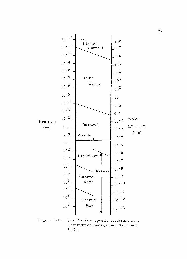
94
a -c Electric
Current
10 -6 -I
Radio Waves
ENERGY (ev) 0.1 -
1. 0 -
10
102
103
104
105
106
107
108
109
Infrared
Visible
108
-107
106
105
104
103
102
10
1.0
0.1
10 -2
10-3
-10-4
- 10 -5
10 -6
10 -7
- 10 -8
10 -9
10 -10
10-11
10 -12
Ultraviolet
'*-----------------... X-rays Gamma
Rays
Cosmic Ray
10 -13
WAVE
LENGTH (cm)
Figure 3 -11. The Electromagnetic Spectrum on a Logarithmic Energy and Frequency Scale.
10 -12_
10 -11-
10-10_
10 -9 - 10 -8 - 10 -7
-
-
-
-
-
l0-5 - 10 -4
10-3 - 10-2 -
- -
-
-
-
-
95
transformation from the unstable to the ground state. With some nu-
clides the consequent gamma emission is delayed considerably (up to
several hours), in which case the "excited state" has a prolonged ex-
istence. Such delayed gamma radiation accounts for isomeric transi-
tions.
Examination of decay schemes will reveal that gamma rays
have discrete energy levels. As is the situation in alpha emission,
this phenomenon is related to discrete energy levels existing within
the nuclear energy well (see Figure 3-1). Gamma rays from most
radioactive nuclides have energies falling in the range between 10
Key to three Mev. A very few range up to seven Mev. Due to alter-
nate pathways of decay, many isotopes emit gamma rays of several
different energy levels (see Figure 2 -4).
c. X -rays: X -rays from radioactive nuclides are commonly
emitted as a result of electron capture and their energies are those
characteristic of the energies of the inner orbital electron levels.
The energy range is from a few ev to about 1 20 Key, quite in contrast
to the gamma energy range. Two common examples are the eight
Key x -rays from Zn65 and the five Key x -rays from Cr51
2. Mechanisms of interaction with matter
Because gamma rays are uncharged and thus carry no

96
appreciable force field with them as they travel through matter, they
cannot bring about direct ionization of atoms in their path. Neverthe-
less, several of their common modes of interaction with matter result
in the consequent ejection of electrons. These ejected electrons,
moving at high velocity, are capable of causing ionization in the sur-
rounding matter. Thus, gamma radiation brings about ionization, but
only in an indirect manner. The direct effect of gamma radiation is
excitation of the nucleus, or orbital electrons with which interaction
occurs.
Like other electromagnetic radiation, gamma rays show wave
behavior in traveling through space. However, when they interact
with matter, they behave as quanta, or "bundles of energy. " Since
this is true, we can reasonably speak of them as "colliding" with parts
of an atom. Their uncharged nature makes such collisions much less
likely than for particulate radiation. This lessened probability of in-
teraction leads to their very high penetrating power. In fact, they
have no clear cut range as such.
Gamma rays interact with matter in at least six different ways.
Three of these are concerned with nuclear interaction and the other
three with orbital electron effects. The first three methods listed
are of only minimal importance in tracer applications of radioisotopes.
a. Nuclear transformation: Very high energy gamma rays
97
(over six Mev) may directly interact with a nucleus, causing excita-
tion of the nucleons. This may result in the ejection of a particle,
usually a neutron, and transmutation of the atom to another nuclide
(a ', n reaction). The energy level required is well above that of
gamma rays from nearly all radioactive nuclides. An exceptional
situation exists in the case of H3,_:r!d e9. These nuclides have photo -
disintegration thresholds of 2. 23 and 1. 67 Mev, respectively. Thus,
a mixture of one of these nuclides with a radionuclide emitting gamma
rays of the requisite energy can serve as a source of neutrons (see
page 30).
b. Mössbauer effect: In certain situations a gamma ray may
be absorbed by a nucleus without consequent particle emission. The
nucleus remains in this excited state for a brief, but measurable
period of time. Subsequent emission of the gamma photon restores
the stability of the nucleus. The atom affected has remained the same
nuclide throughout this process. There has been no transformation
in this case. This type of interaction may be described as nuclear
resonance scattering.
c. Bragg scattering (diffraction): Low energy gamma rays
may be scattered from a crystal face with no loss of energy. Such an
x -ray diffraction effect is used effectively in the study of crystal
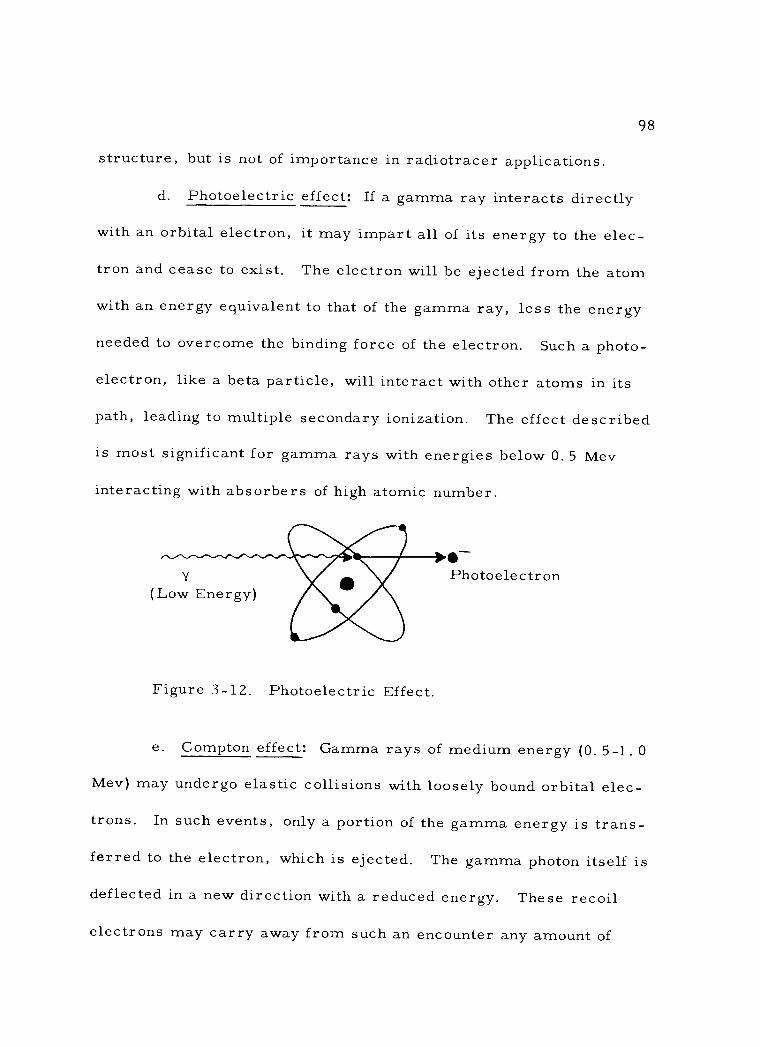
98
structure, but is not of importance in radiotracer applications.
d. Photoelectric effect: If a gamma ray interacts directly
with an orbital electron, it may impart all of its energy to the elec-
tron and cease to exist. The electron will be ejected from the atom
with an energy equivalent to that of the gamma ray, less the energy
needed to overcome the binding force of the electron. Such a photo-
electron, like a beta particle, will interact with other atoms in its
path, leading to multiple secondary ionization. The effect described
is most significant for gamma rays with energies below 0. 5 Mev
interacting with absorbers of high atomic number.
N
(Low Energy)
Figure 3 -12. Photoelectric Effect.
Photoelectron
e. Compton effect: Gamma rays of medium energy (0. 5 -1 . 0
Mev) may undergo elastic collisions with loosely bound orbital elec-
trons. In such events, only a portion of the gamma energy is trans-
ferred to the electron, which is ejected. The gamma photon itself is
deflected in a new direction with a reduced energy. These recoil
electrons may carry away from such an encounter any amount of
99
energy up to a fixed maximum. Thus, Compton recoil electrons ap-
pear with a wide energy spread even from a monoenergetic beam of
incident gamma radiation. Considerable secondary ionization can be
produced as these electrons dissipate their energy. Moreover, the
attenuated gamma ray may undergo several more such collisions be-
fore it finally loses all its energy. The Compton effect is favored
for gamma rays of medium energy interacting with absorbers of me-
dium to low atomic number.
Y
(Medium Energy)
Figure 3 -13. Compton Effect.
Y
(Reduced Energy)
Recoil Electron
f. Pair production: A unique phenomenon may occur when a
gamma ray interacts directly with the nuclear force field. In such
an event, the photon may cease to exist and have all its energy con-
verted into two particles, a positron and an electron, which are eject-
ed from the site with varying energy. In order for this to take place,
the incident gamma ray must have an energy equal to, or greater
than 1. 02 Mev, which is the energy equivalent to the rest mass of two
100
electrons. This occurrence illustrates the interconvertibility of
energy and mass. The positron produced quickly undergoes annihila-
tion, with consequent back -to -back gamma emission. On the other
hand, the ejected electron may cause ionization of atoms near its
path. Pair production increases proportionately to the atomic num-
ber of the absorber and, above the absolute minimum level of 1. 02
Mev, increases proportionately to the energy of the incident gamma
photon.
Y
(E > 1. 02 Mev)
Figure 3 -14. Pair Production.
Positron (Annihilated)
In summary, the latter three methods of interaction (photo-
electric effect, Compton effect, pair production) are the principle
ways in which gamma energy from radionuclides is dissipated. It is
the ionization effects of the secondary electrons produced by gamma
absorption that are more readily detected than the primary gamma
photons themselves.
Electron
101
3. Absorption relations
a. Linear absorption: Since the absorption of gamma radia-
tion is exponential in nature, gamma rays have no clearcut range.
This is in contrast to alpha and beta radiation. In order to examine
certain quantitative aspects of gamma absorption, an ideal absorption
situation is pictured (Figure 3 -15), in which a collimated beam (all
parallel rays) of gamma radiation is incident on a thin slab of absor-
ber material.
......... ..r--ti..-- -. ...r._ .-
//'/ElV`
Y Intensity = to Thickness 0 X
Y Intensity = Io - DI
Figure 3 -15. Gamma Ray Absorption.
As the incident gamma beam of intensity I 0 passes through the
thin absorber with a thickness OX, some of the gamma rays are ab-
sorbed resulting in a decline in gamma intensity equal to AI. Io
minus AI then equals the intensity of the emerging gamma beam. It
should be clear that the thicker the absorber, the greater will be the
---
....__
=
102
absorption. Thus, the fraction of the beam intensity absorbed is pro-
portional to the thickness of the absorber through which it passes, or:
(Equation 3 -4) DI a OX Io
This expression can be made into an equation by introducing
a constant µI , the linear absorption coefficient, which represents
the fractional decrease in gamma intensity per unit thickness of ab-
sorber.
(Equation 3 -5) DI = -µ.Q
Io
The minus sign indicates that a decrease in intensity is occurring.
Since absorption is a continuous process through the slab,
rather than an incremental process, an infinitesimal absorber thick-
ness (dx) must be substituted. Integration of the resulting equation
yields
(Equation 3-6) logo 4_0 = - µ X
In this equation, Io represents the incident gamma beam intensity,
while I stands for the intensity that will emerge from an absorber of
x thickness. Converting the equation from natural logarithms to corn -
mon logarithms (1°g1 0) gives
Io

(Equation 3 -7) I log 0
Io log -
I
= -0. 434 µl x, or
= 0. 434 µ X
103
The linear absorption coefficient is commonly expressed per
centimeter (1 /cm). Its value depends on two factors: the energy of
the gamma rays involved, and the type of absorber material used.
These relationships are seen in the values listed in Table 3 -3.
Table 3 -3. Linear absorption coefficients per cm for selected absorbers.
Incident gamma energy H20 Al Fe Pb
1. 0 Mev 0. 071 0. 168 0. 44 0. 79
1. 5 Mev 0. 057 0. 136 0. 40 O. 590
2. 0 Mev 0. 050 0.117 0. 33 O. 504
Example: What fraction of a 1. 5 Mev gamma beam will pass
completely through a five cm thick lead brick? The µ/ for 1. 5 Mev
gamma in lead equals 0. 590 /cm.
(Equation 3-8) log 1 00
I 0. 434 x 0. 590/cm x 5 cm
log 1. 00 - log I = 1. 28
Io

log I = -1. 28
". = 0.052, or - 5%
104
b. Mass absorption: As can be seen in Table 3 -3, the linear ab-
sorption coefficient varies considerably for different absorber mate-
rials. By taking the density of the absorbing material into account, a
more comparable unit can be derived. In considering a volume of ab-
sorber that is one cm2 in cross section and X cm long, the volume is
numerically equal to the length (x). The mass in this volume equals
the density (p) times the length (px). It follows that the fractional
gamma absorption is proportional to the mass of absorber traversed.
Substitution of p OX in place of AX in Equation 3 -4 gives
(Equation 3 -9) DI a. pAX
Io
In order to make an equation from this expression, the mass
absorption coefficient (µ ) is introduced. It is simply the linear ab- m
sorption coefficient divided by the density of the absorber or:
(Equation 3-10) µ m
FI p
Once again, integration of the resulting equation gives
(Equation 3-11) log I = -µ pX n I m
0
=

105
It will be seen that this equation is quite similar to Equation 3 -6. In
the one, absorption is calculated from the mass absorption coefficient
times mass, while in the other it is calculated from the linear absorp-
tion coefficient times linear thickness.
As will be noted in Table 3 -4, the mass absorption coefficients
are quite similar for gamma rays of the energies listed in all absor-
bers. This near independence of the nature of the absorber makes
this unit roughly comparable. Although mass absorption coefficients
are commonly expressed in units of cm2 /g, they are also shown as
Table 3 -4. Mass absorption coefficients in cm2 /g.
Incident gamma energy H20 Al Fe Pb
1.0 Mev . 071 . 062 . 062 . 070
1.5 Mev . 057 . 050 . 056 . 052
2. 0 Mev . 050 . 043 . 046 . 046
cm2 /mg on occasion. An additional advantage of the mass absorption
coefficient is that it is independent of the chemical or physical state
of the absorber. The value for liquid water and water vapor is the
same, whereas the µ/ values would differ greatly.
Example: What fraction of gamma radiation from a 1 Mev
beam would completely pass through two centimeters of lead under

106
ideal conditions? The µm value for 1 . 0 Mev gammas in lead is 0. 07
cm2 /g, and the density of lead is 11.3 g /cm3.
(Equation 3-1 2) log1 1 i00 _ 0. 434 x 0. 07 cm2/g x 11. 3 gm/cm3
x 2. 0 cm
log 1. 00 - log I = 0. 678
log I = -0. 678 = 9. 322 - 10
I = 0. 210 or 21%
Two other absorption coefficients are used, though not com-
monly. The atomic absorption coefficient (µa) takes into account the
actual number of atoms in the absorbing material and is equivalent to
the fraction of energy absorbed per single atom in the absorber.
Since low energy gamma rays interact predominantly with the orbital
electrons, the electronic absorption coefficient (µe) is occasionally
employed. It represents the fraction of intensity absorbed by indivi-
dual electrons in the absorber.
c. Half thickness: Absorption curves plotted for gamma in-
tensity versus the thickness (or mass) of the absorber appear in
Figure 3 -1 6. From the semi -log curve (B) another convenient ex-
pression of the exponential absorption process can be visualized.
This is the half thickness (X1 /2) or "half value layer ", defined as the
thickness of absorber material which will reduce the incident
=
-
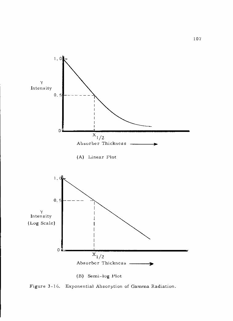
107
Intensity
X12 Absorber Thickness
(A) Linear Plot
0. 5
Y Intensity
(Log Scale)
X12 Absorber Thickness
(B) Semi -log Plot
Figure 3 -16. Exponential Absorption of Gamma Radiation.
Y
1.0
0.5
--
108
radiation intensity by a factor of two. The parallel here to the expon-
ential nature of radioactive decay and half -life should be noted. Half
thickness is a unit of convenience and utility in calculating the shield-
ing necessary to reduce gamma ray intensity to desired levels.
Half thickness can be defined either as linear half thickness or
mass half thickness. For the same reasons outlined above concerning
the mass absorption coefficient, the mass half thickness is the more
useful unit. The mass half thickness can be derived from Equation
3-11, where p x equalled the mass of the absorber. If the gamma
radiation intensity is to be reduced by a factor of two, the following
equations would result:
(Equation 3-13) Io/2 A. logn
Io
B. logn 2
C X 0. 693 1/2
m
From this it will be seen that the value of the mass half thickness can
be directly calculated from the mass absorption coefficient.
In gamma ray shielding problems, the use of the mass half
thickness allows rapid calculation of the approximate shielding neces-
sary to reduce personnel exposure to gamma radiation. If one half
thickness will reduce gamma intensity to one half its original value,
µmx
P.
= -µmX/2
_
109
then two half thicknesses will reduce it to one fourth, etc. The num-
ber of half thicknesses (N) of absorber required to reduce gamma in-
tensity by the factor of X would be equivalent to a total absorber mass
of d'. The value of N can be readily derived from Equation 3 -13 B.
First, by substitution,
(Equation 3 -14) logn X = µmd'
Introducing the value of µm from Equation 3 -13 C. gives
(Equation 3 -15) logn X - 0. 693 d', X1 /2
but since N = d' /X1 this can be reduced to
(Equation 3 -16) logn X = 0. 693 N
Converting to common logarithms and solving for N yields
(Equation 3-1 7) N = 3. 33 1og10 X
This reduces simple shielding determination to a straightforward
calculation. Thus, when it is desired to reduce the gamma intensity
to 1/8th,
(Equation 3 -1 8) N = 3. 33 logt 8 = 3.0 half thicknesses required.
d. Dependence on gamma energy and absorber density: The
exponential nature of gamma absorption is evident from Figure 3 -1 6 B.
m
110
The absorption equations used above (Equations 3 -6 and 3 -11) can
also be expressed in an exponential form similar to that used for
radioactive decay (Equation 2 -8):
-µx (Equation 3-19) I = Io e
(Equation 3-20) I = Io e -µm x
(linear absorption)
(mass absorption)
The symbol e used in these equations stands for the value 2. 71 8, the
base of the natural logarithms.
It is quite remarkable that gamma absorption should be expon-
ential, in view of the fact that it is actually due to six distinctly dif-
ferent processes. Of these six interaction processes, only three
(photoelectric effect, Compton effect, and pair production) are nor-
mally significant at the gamma energies associated with most nuclides
used in radiotracer applications. Each of these processes is highly
dependent on the gamma energy involved, and the density of the ab-
sorber used. This energy dependence is clearly seen in Figure 3 -17,
which indicates the plot of µm values against gamma energy for the
three significant gamma interaction processes.
It will be noted that the photoelectric effect is most pronounced
at lower energies, the Compton effect is the predominant interaction
type at intermediate energies, and pair production becomes an
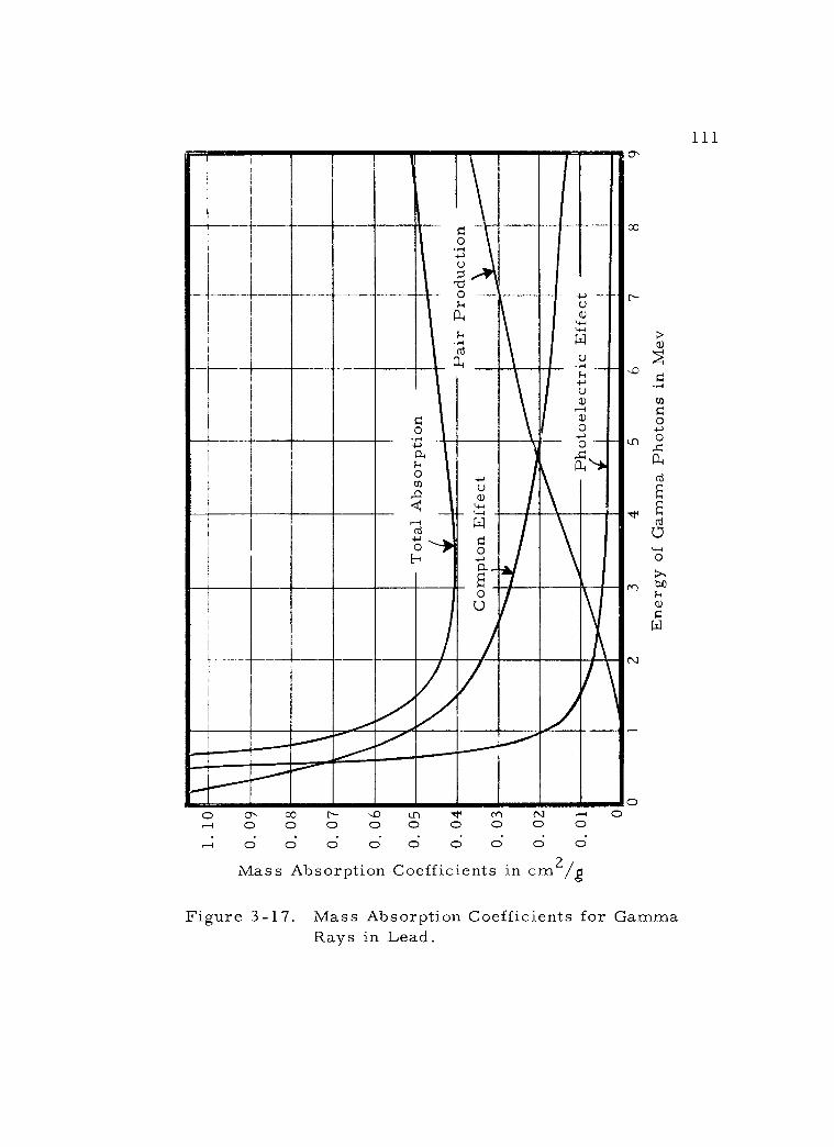
1.
10
0. 0
9 C
B
--.1
y
0.08
o-
'
w
° 0.
07
u)
u)
U)
' 0
0.06
t'
ci)
n ¢,
°
0.05
0. 0
4
0 .
0 3
0.02
D
N
o oI
0.
01
1-1 C) P ó n o , , o
H. ,-.
<,-
u)
n
1 iilL
Iw
o A
bsor
ptio
n T
otal
Pair
Pro
duct
ion
Com
pton
Eff
ect
0..-
E
ffec
t L
. Ph
otoe
lect
ric
----
, ï
0 1
2 3
4 5
6
Ene
rgy
of G
amm
a Ph
oton
s in
Mev
7
8
r
i
(D
CI)
r
r í
rr
\ 0
____
____
____
a
_ _
w
w
g w
1t
Td r-
9
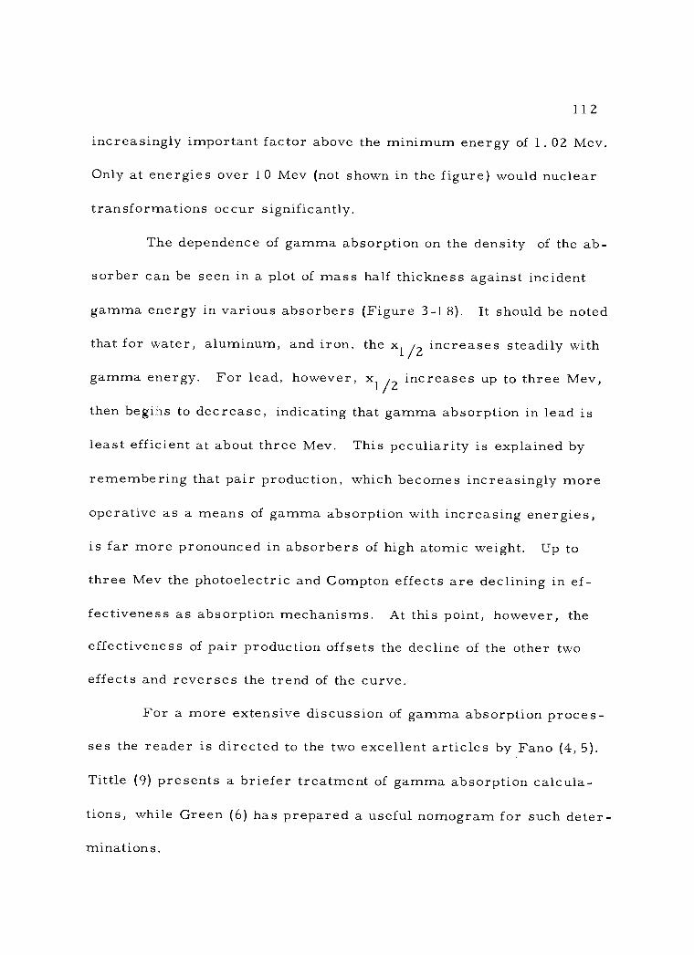
112
increasingly important factor above the minimum energy of 1.02 Mev.
Only at energies over 10 Mev (not shown in the figure) would nuclear
transformations occur significantly.
The dependence of gamma absorption on the density of the ab-
sorber can be seen in a plot of mass half thickness against incident
gamma energy in various absorbers (Figure 3 -1 8). It should be noted
that for water, aluminum, and iron, the x1/2 increases steadily with
gamma energy. For lead, however, x1 increases up to three Mev,
then begins to decrease, indicating that gamma absorption in lead is
least efficient at about three Mev. This peculiarity is explained by
remembering that pair production, which becomes increasingly more
operative as a means of gamma absorption with increasing energies,
is far more pronounced in absorbers of high atomic weight. Up to
three Mev the photoelectric and Compton effects are declining in ef-
fectiveness as absorption mechanisms. At this point, however, the
effectiveness of pair production offsets the decline of the other two
effects and reverses the trend of the curve.
For a more extensive discussion of gamma absorption proces-
ses the reader is directed to the two excellent articles by Fano (4, 5).
Tittle (9) presents a briefer treatment of gamma absorption calcula-
tions, while Green (6) has prepared a useful nomogram for such deter-
minations.
113
0 0.2 0.5 1. 0 1 5 2 0 2.5 3. 0
Gamma Photon Energy 4. 0
Figure 3 -18. Relation Between X1 and Gamma Energy in
Various Absorbers.
5. 0
114
The general features of gamma absorption also apply to x -ray
absorption. The major difference is that x -rays are not emitted from
radionuclides with sufficient energy to cause pair production. Be-
cause the x -ray energies are generally low, diffraction is a more
significant phenomenon. This latter characteristic is utilized in the
study of crystalline structure. The diffraction pattern produced when
a beam of soft x -rays strikes a crystal face permits a very exact
determination of the spacings of atoms within the crystal.
4. Practical considerations
The presence of even moderate quantities of gamma emitting
nuclides in a laboratory poses a problem because of the highly pene-
trating nature of gamma radiation. The isotopic material must com-
monly be stored in a shielded container of lead or other dense mate-
rial. If the radiation level is sufficiently high, manipulation of the
gamma emitting material may require shielding and /or remote con-
trol apparatus of a simple type. The external hazard from gamma
emitting radionuclides is quite in contrast to that from alpha and beta
emitters. The entire volume of body tissue can be irradiated from
an external gamma source. When taken internally, gamma emitters
can produce essentially whole body radiation effects, even though
largely localized. The presence of gamma emitting nuclides in the
115
laboratory likewise tends to increase the normal background radiation
level, with deleterious effects on radiotracer assay.
In the detection of gamma rays, interaction is such that the
gas -filled chambers used to detect alpha and beta radiation are most
inefficient. It is desirable to use detectors of great density for maxi-
mum absorption. Sodium iodide crystals are the substances most
generally employed for this purpose. The excitation energy from ab-
sorbed gamma quanta in such a crystal is emitted as minute flashes
of visible light (photons). These scintillations may be converted to
an electron flow, which can be amplified and measured (see Chapter
5).
D. Summary
In summary, it will be recalled that alpha and beta particles
cause primary ionization as they interact with matter. On the other
hand, gamma radiation produces only a primary excitation, with ioni-
zation only a secondary effect. Alpha and beta radiation will be re-
membered as charged particles, whereas gamma radiation consists
of electromagnetic quanta. The range of alpha particles is quite dis-
crete, that of beta particles is not as well defined, while gamma ra-
diation has no clearly delimited range, but is continuously absorbed
on an exponential basis.
116
BIBLIOGRAPHY
1. Barreira, F. and M. Laranjeira. A graphical absolute method for range determination of n- particles. The International Journal of Applied Radiation and Isotopes 2:145 -148. 1 957.
2. Brownell, Gordon L. Interaction of phosphorus -32 beta rays with matter. Nucleonics 1 0(6) :30 -35. 1 952.
3. Duncan, J. F. and F. G. Thomas. Three beta -absorption methods - -- how do they compare? Nucleonics 15(10) :82 -85. 1957.
4. Fano, U. Gamma -ray attenuation. Part I. Basic processes. Nucleonics 11 (8):8 -1 2. 1 953.
5. Fano, U. Gamma -ray attenuation. Part II. Analysis of penetra- tion. Nucleonics 11 (9):55 -61 . 1 953.
6. Green, Marvin H. Absorption of mono -energetic x- and y - rays. Nucleonics 1 7(1 0) :77. 1 959.
7. Katz, L. and A. S. Penfold. Range- energy relations for elec- trons and the determination of beta -ray end -point energies by absorption. Reviews of Modern Physics 24(1 ):28 -44. 1 952.
8. Marshall, John H. How to figure shapes of beta -ray spectra. Nucleonics 1 3(8):34 -38. 1 955.
9. Tittle, C. W. How to compute absorption and backscattering of gamma rays. Des Plaines, Ill. , 1 960. 4 p. (Nuclear - Chicago Technical Bulletin No. 9)
CHAPTER 4 - MEASUREMENT OF RADIOACTIVITY: GENERAL CONSIDERATIONS AND THE METHOD BASED
ON GAS IONIZATION
A. Absolute Counting vs. Relative Counting
1. Types of radioactivity measurements
117
The detection and measurement of radioactivity may be carried
out on several different bases. In absolute counting, every disintegra-
tion occurring in the sample is accounted for and the results are hence
expressed in disintegrations per minute (dpm). On the other hand,
radioactivity may be measured on the relative counting basis, where
only a given fraction of the true disintegration rate of the sample is de-
tected. A specific proportionality can be maintained between this rela-
tive counting rate and the absolute counting rate in a series of samples
by utilizing identical counting conditions. In this way, repeated rela-
tive counts will be comparable to one another. The results of relative
counting are usually stated as counts per minute (cpm).
The foregoing description of the measurement of radioactivity
is not to be confused with the measurement of radiation dose. Abso-
lute and relative counting pertain to detecting and measuring events,
while dosimetry is concerned with measuring the energy dissipation
and absorption in a defined system. The radiation dose depends
-
118
heavily on the energy and type of the incident radiation and the nature
of the absorbing material; hence, precise determinations are much
more difficult to make. Radiation dose values are commonly given in
roentgen or rad units (see Chapter 1 2).
The purposes and applications of these three types of measure-
ment are quite different. Radiation dosimetry, being concerned with
the absorption of radiation energy, is of importance chiefly to radia-
tion biologists and health physicists. Further discussion of this aspect
will be found in Chapter 1 2. Absolute counting, where the true radio-
active disintegration rate is measured, is employed in precise studies
of such nuclear phenomena as the determination of long half -lives, and
in the preparation of radioactive standard sources for instrument cali-
bration. It is used largely by physicists, nuclear reactor personnel,
and radiochemists. Thus, it will not be discussed in the present book
beyond this point. Relative counting is of primary importance in radi-
otracer methodology and, consequently, will be discussed in this and
the following chapters.
2. Considerations in relative counting
In order for relative count rate determinations to be truly
comparable from one sample to another, careful attention must be giv-
en to the preparation of the radioactive samples. The mounting of the
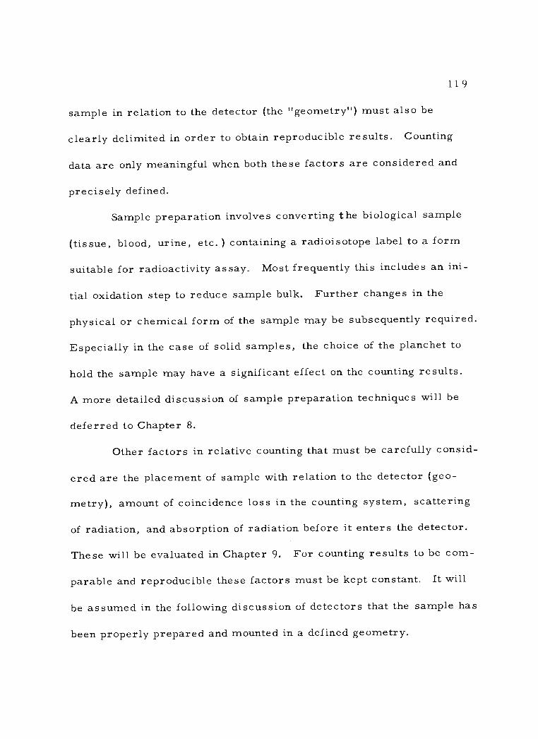
119
sample in relation to the detector (the "geometry ") must also be
clearly delimited in order to obtain reproducible results. Counting
data are only meaningful when both these factors are considered and
precisely defined.
Sample preparation involves converting the biological sample
(tissue, blood, urine, etc. ) containing a radioisotope label to a form
suitable for radioactivity assay. Most frequently this includes an ini-
tial oxidation step to reduce sample bulk. Further changes in the
physical or chemical form of the sample may be subsequently required.
Especially in the case of solid samples, the choice of the planchet to
hold the sample may have a significant effect on the counting results.
A more detailed discussion of sample preparation techniques will be
deferred to Chapter 8.
Other factors in relative counting that must be carefully consid-
ered are the placement of sample with relation to the detector (geo-
metry), amount of coincidence loss in the counting system, scattering
of radiation, and absorption of radiation before it enters the detector.
These will be evaluated in Chapter 9. For counting results to be com-
parable and reproducible these factors must be kept constant. It will
be assumed in the following discussion of detectors that the sample has
been properly prepared and mounted in a defined geometry.

1 20
B. Basic Mechanisms of Radiation Detection
It was seen in the previous chapter that alpha, beta, and gam-
ma radiation can interact with matter in a variety of ways. Of these
types of interaction, those which ionize gas atoms, cause orbital elec-
tron excitation in solids or liquids, or induce specific chemical reac-
tions in sensitive emulsions are most commonly utilized in the detec-
tion of radiation. The detectors themselves will be described in de-
tail after a brief survey of the mechanisms involved.
1. Gas ionization
Several detector types take advantage of the ionizing effect of
radiation on gases. The ion pairs so produced can be separately col-
lected. When a potential gradient is applied between the two elec-
trodes in a gas- filled ion chamber the positively charged molecules
move to the cathode and the negative ions (electrons) move swiftly to
the anode thereby creating a measurable pulse. Such pulses can be
readily measured by the associated devices as individual events or
integrated current.
2. Scintillation
a. In a solid fluor: A portion of the energy of ionizing
121
radiation can he transferred to fluor molecules in a crystalline
solid. The absorbed energy causes excitation of orbital electrons in
the fluor. De- excitation gives rise to the emission of the absorbed
energy as electromagnetic radiation (scintillations) in the visible or
near ultraviolet region. While it is possible to observe these weak
scintillations visually under certain circumstances, visual observa-
tion is not normally a feasible detection method. Instead, a photomul-
tiplier tube in close proximity to the solid fluor is employed. In this
photomultiplier the energy of the photons is first transferred to photo-
electrons, and then greatly amplified by secondary electron emission
through a series of electrodes (dynodes). In this way the original ex-
citation energy is transformed into a measurable pulse. This means
of detection is further described in Chapter 5.
b. In a liquid fluor: This detection mechanism is quite simi-
lar in principle to that above. Here, however, the radioactive sample
and fluor are intimately in contact in a liquid medium, usually a non -
polar solvent. The excitation energy is transferred first to the sol-
vent molecules and then to the dissolved fluor, which in turn emits
photons. These photons are detected by means of the same photomulti-
plier arrangement as described immediately above. Further discus-
sion of the detection method will be found in Chapter 6.

122
3. Autoradiography
This mechanism is a photochemical process. A sample con-
taining radioactivity is placed in close contact with a photographic
emulsion on film. Ionizing radiation from the sample interacts with
the silver halide grains in the emulsion to bring about a photochemical
reaction. Subsequent development of the film produces an image and
hence permits a semi- quantitative estimation of the radiotracer in the
sample. Historically, this is the way in which radioactivity was first
detected (by Becquerel in 1896). Autoradiographic detection can be
employed with a minimum of specialized apparatus, whereas detectors
using gas ionization or the scintillation mechanisms usually require
one or more associated electronic devices. Chapter 7 includes a more
detailed discussion of autoradiography.
C. Gas Ionization
As an energetic charged particle passes through a gas, its
electrostatic field will dislodge orbital electrons from atoms suffici-
ently close to its path. In each case, the negatively charged electron
dislodged and the more massive positive ion comprising the remainder
of the atom form an ion pair. The minimum energy (in ev) required
for such ion pair formation in a given gas is called the ionization
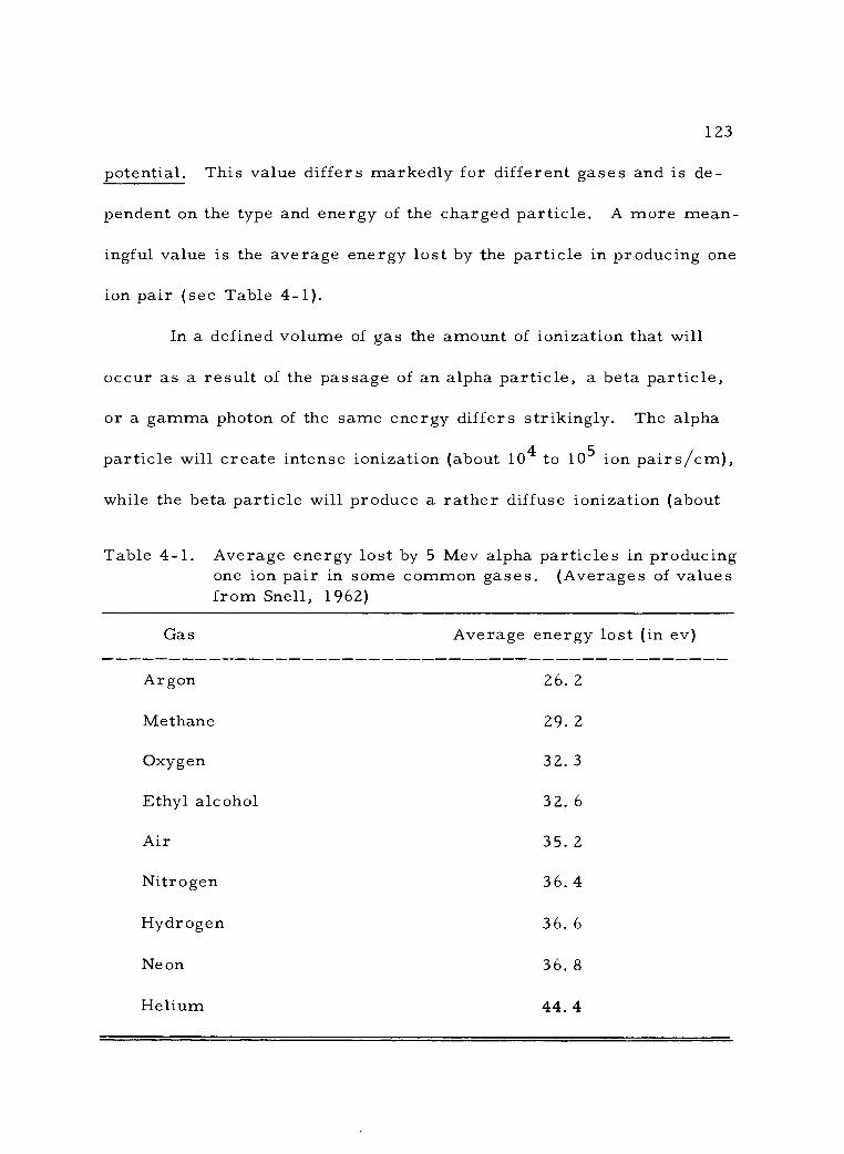
123
potential. This value differs markedly for different gases and is de-
pendent on the type and energy of the charged particle. A more mean-
ingful value is the average energy lost by the particle in producing one
ion pair (see Table 4 -1).
In a defined volume of gas the amount of ionization that will
occur as a result of the passage of an alpha particle, a beta particle,
or a gamma photon of the same energy differs strikingly. The alpha
particle will create intense ionization (about 104 to 105 ion pairs /cm),
while the beta particle will produce a rather diffuse ionization (about
Table 4 -1. Average energy lost by 5 Mev alpha particles in producing one ion pair in some common gases. (Averages of values from Snell, 1962)
Gas Average energy lost (in ev)
Argon 26. 2
Methane 29. 2
Oxygen 32. 3
Ethyl alcohol 32. 6
Air 35. 2
Nitrogen 36. 4
Hydrogen 36. 6
Neon 36. 8
Helium 44. 4

124
102 to 103 ion pairs /cm), and the gamma ray will interact very little,
if at all (about 1 to 10 ion pairs /cm), and that by secondary mecha-
nisms. Accordingly, it can be seen that alpha and beta particles pro-
duce sufficiently intense specific ionization for detection, but gamma
rays are poorly detected at best by this means.
1. Without gas amplification
a. Ionization chambers in general: A chamber for ion collec-
tion may consist of a cylindrical closed metal container filled with air,
or some other gas, and fitted with a central collecting electrode, as
illustrated in Figure 4 -1. The chamber wall is connected to the nega-
tive pole of a potential source making it the cathode, while the collect-
ing electrode is connected through a resistor to the positive side of
the power supply, so that it serves as the anode. The collecting elec-
trode is carefully insulated from the chamber wall. A capacitor is in-
cluded in the circuit in such a way that it will be charged by a current
originating at the collecting electrode.
Now, if a 3. 5 Mev alpha particle is allowed to enter the cham-
ber, intense ionization will occur along its short path. Since about 35
ev are expended on the average in forming an ion pair in air, the 3. 5
Mev alpha particle could form approximately 1 x 10⁵ such ion pairs
before dissipating all its energy. Due to the potential impressed on
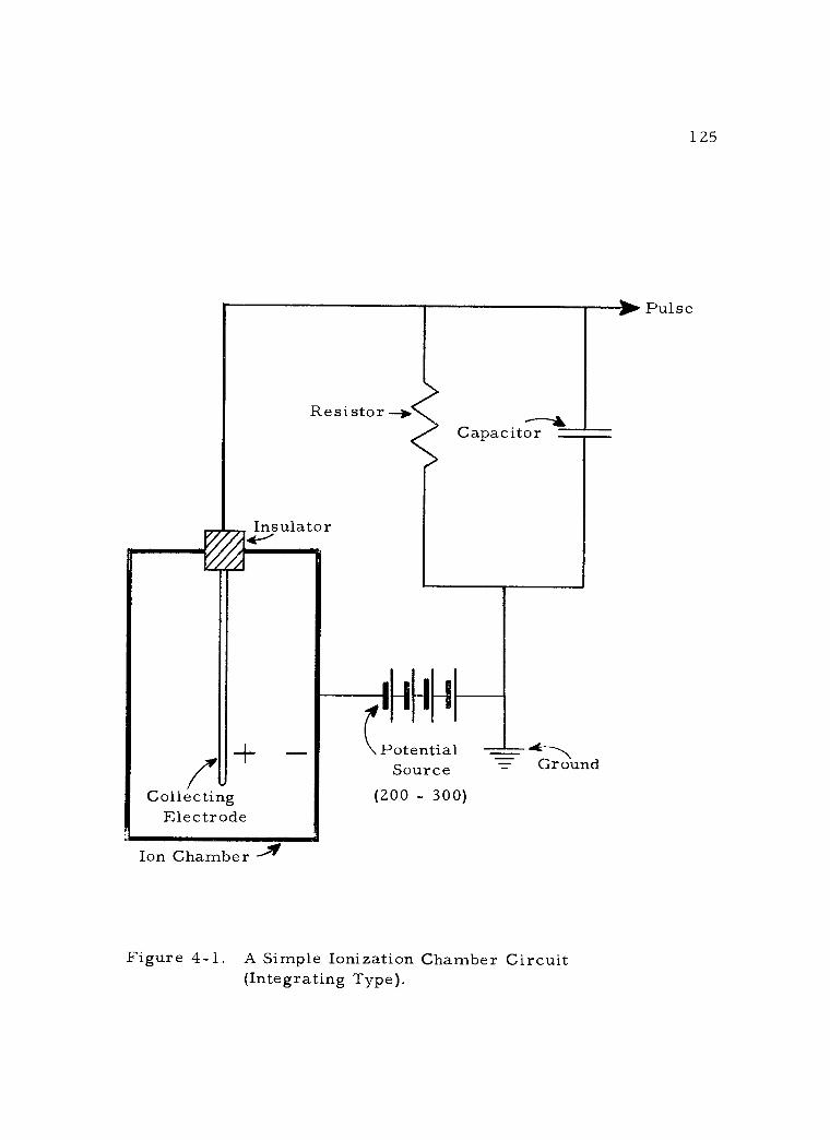
Resistor -k
Insulator t 41-
Collecting Electrode
Ion Chamber
---y Capacitor
Potential Source
(200 - 300)
Ac-------,,
znd
Figure 4 -1. A Simple Ionization Chamber Circuit (Integrating Type).
125
Pulse
1
126
the chamber electrodes, these ions migrate rapidly to the respective
electrodes. The lighter electrons move more quickly to the central
collecting anode and produce a rapid build -up of charge there. The
magnitude of this charge can be calculated as follows:
(Equation 4-1) One e- charge = 1. 6 x 10 -19 coulombs
1 x 10⁵ e- x 1. 6 x 10-19 coulombs /e- =
1. 6 x 10 -14 coulombs
The collected charge flows through the external circuit as a surge, or
pulse. If a 20 µµf capacitor is being used, the potential of the pulse is
found as follows:
Charge in Coulombs (Equation 4 -2) = Pulse size in volts Capacitor size in Farads
1. 6 x 10 -i4 coulombs = 8 x10⁻⁴ volts, or .0008 volts
2. 0 x 10 -i1 farads
The precise measurement of such minute pulses constitutes a basic
difficulty in using the simple ionization chamber for the detection of
ionizing radiation.
If, instead, a beta emitting source is brought near the ioniza-
tion chamber, a much smaller degree of ionization will occur along
beta tracks in the chamber. It is not possible to calculate the actual
number of ion pairs that will be formed for an individual beta particle
and the consequent charge collected since beta particles are emitted
127
over a continuous energy spectrum. The mean kinetic energy associ-
ated with beta particles is generally much lower than with alpha parti-
cles and the specific ionization of beta particles is inherently low. As
a result, the size of pulse produced by an individual beta particle will
be smaller by a hundred or a thousand fold than that produced by an
alpha particle. Gamma rays produce only secondary ionization and
have such very low specific ionization that the pulse produced is very
small indeed.
Up to this point, it has been merely stated that a potential is
applied across the electrodes of the ionization chamber. The relation-
ship between the potential in the ionization chamber and the amount of
charge collected on the anode will now be examined. If no potential is
applied, a negligible charge will be collected, although ionization does
occur in the chamber. Recombination of the ions will take place ra-
pidly in the wake of the ionizing particle. At only a few volts potential,
some ions will be collected, but most will still recombine before
reaching the electrodes. Continued increase in potential gradient will
result in an increasingly larger fraction of the ions being collected,
until eventually all ions are collected and virtually no recombination
occurs. From this point an increase of chamber potential over per-
haps several hundred volts gives essentially no increase in charge
collected. Under these conditions a saturation current is realized at
128
the collecting electrode. Ionization chambers are usually operated to-
ward the middle of the saturation current region, so that any fluctua-
tion in the supplied potential will not affect the ion current. Figure
4 -2 shows this relationship. One advantage of the simple ionization
chamber, then, is that a highly stable chamber potential supply is not
required.
Up to this point, only a single surge of current produced by a
solitary ionizing particle has been discussed. Of course, a radioac-
tive sample will be emitting particles continuously into an ion cham-
ber, so that volleys of pulses will be initiated in the external circuit.
These pulses may be recorded in two different manners. The indivi-
dual pulses may be tallied to give a record of the number of ionizing
particles entering the chamber (a differentiating circuit). Because
of the pulse size involved, such a method is generally feasible only
for alpha particles, and has the disadvantage of requiring an elaborate
pulse amplifier. Consequently, some type of integrating circuit is
most commonly employed with a simple ionization chamber. In this
way, the total current flow over a given time interval is measured,
rather than the discrete pulses. This total ion current is proportional
to the degree of ionization occurring in the chamber during the time
interval. Two major types of integrating instruments are currently in
common use. These are electroscopes and electrometers. An
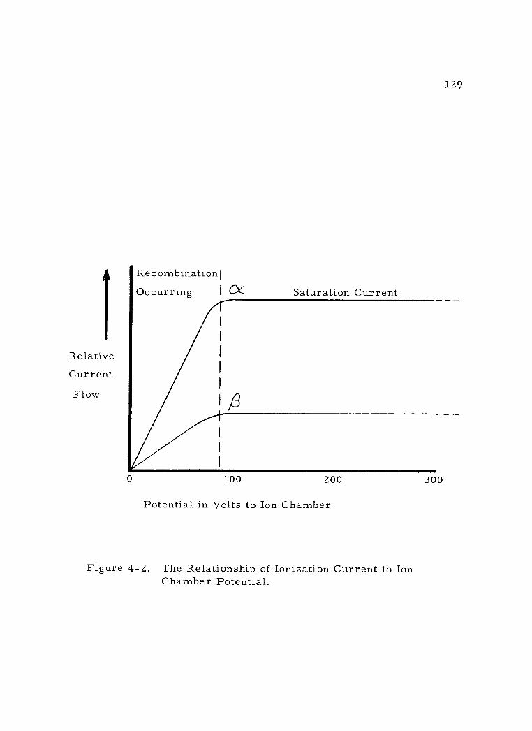
T
Relative
Current
Flow
Recombination
Occurring
129
I OC Saturation Current
100 200 300
Potential in Volts to Ion Chamber
Figure 4 -2. The Relationship of Ionization Current to Ion Chamber Potential.
130
example of each type that may be used for radiotracer assay will be
described in detail below.
b. Lauritsen electroscopes: The Lauritsen electroscope is
merely a highly refined version of the classic gold -leaf electroscope.
In this instrument the total ionization is integrated over a defined pe-
riod of time. The details of this type of electroscope are seen in
Figure 4 -3. Within the ionization chamber an insulated L- shaped wire
supports a delicate gold -plated quartz fiber. A microscope tube is so
mounted that the end of the quartz fiber is in focus against a transpar-
ent scale. The quartz fiber and supporting wire assembly are charged
by an external battery through a charging terminal. When charged,
the end of the flexible quartz fiber is repelled by the supporting wire.
As a source of ionizing radiation is brought near and ionization occurs
within the chamber, the ions are collected on the quartz fiber assem-
bly. This reduces its charge and the quartz fiber moves back toward
the supporting wire. This motion can be observed against the scale.
The rate of this movement is directly proportional to the amount of
ionization occurring in the ionization chamber during the observation
period.
Electroscopes are not in common use for radiotracer assay be-
cause of the length of time required for each determination. This type
of instrument, however, has the advantage of being capable of
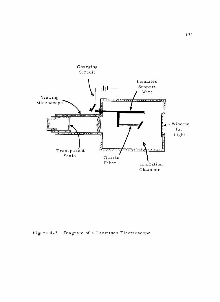
Viewing Microscope
Charging Circuit
Insulated Support
Wire
Transparent Scale Quartz
Fiber Ionization Chamber
Figure 4 -3. Diagram of a Lauritsen Electroscope.
131
Window for
Light
. . .ii.F-. b.il!
-.
132
measuring respectable levels of activity without being overwhelmed
(in contrast to the common Geiger- Mueller counter) and can be con-
structed in a readily portable form. Since the electroscope measures
total ionization occurring per unit time, it is useful for determinations
of radiation dose. It is not surprising to find that the familiar pocket
dosimeter, worn by personnel in radiation hazard areas, is essentially
a miniaturized version of the electroscope described above.
c. Vibrating -reed electrometers: In the second major type of
integrating instrument, the electrometer, the current from the ioniza-
tion chamber is amplified and measured. Several methods of achieving
the degree of amplification required are available. Those which use
direct vacuum -tube amplification find frequent application in portable,
battery- operated monitoring devices. However, these lack the degree
of precision needed for radiotracer assay in the laboratory. This is
due largely to the inherent instability of d -c amplifiers when used with
such extremely small ion currents.
The vibrating -reed electrometer, also known as a dynamic ca-
pacitor electrometer, circumvents the problem of amplifying small
d -c currents. In this instrument one plate of the dynamic capacitor is
mechanically driven so that it vibrates at a frequency of several hun-
dred cycles per second. The direct current from the ionization cham-
ber flows into this continuously varying capacitor and, accordingly,
133
an alternating current is produced. This alternating current may now
be amplified by a stable a -c amplifier, and then rectified.
The magnitude of the amplified ion current from the ionization
chamber may be determined by one of two methods. First, the cur-
rent may be passed through a calibrated resistor, and the equilibrium
voltage across the resistor measured. Secondly, the ion current may
be allowed to charge a calibrated capacitor, and the rate of charge
across the known capacitor measured. In general, the first method of
measurement (potential -drop) is used with large ion currents, while
the second (rate -of- charge) is used where highest sensitivity is de-
sired. In either method some calculation is necessary to equate the
current measurements observed with the amount of activity present in
the sample being assayed.
The vibrating -reed electrometer system has several note wor-
thy features. It allows highly precise measurements to be made over
a wider range of sample activities (5 x 10 -5 to 103 µc) than any other
type of detector. The versatility of this detector is shown by the fact
that solid, liquid, or gaseous samples can be accommodated. How-
ever, for maximum counting efficiency the ion chamber is filled with a
stationary or flowing gaseous sample. In practice these gaseous sam-
ples have been almost entirely limited to C14- or H3- labelled com-
pounds, since biological samples containing them can usually be

134
readily transformed into the gas phase. The counting efficiency for
stationary gas samples of such low energy beta - emitting isotopes ap-
proaches 100 percent. When measurements of flowing gas samples
are made the counting efficiency is heavily dependent on both flow rate
and ion chamber volume, and is usually somewhat lower than for sta-
tionary samples.
A common use of the electrometer system is to measure C14O
in the respiratory flow of air from an organism metabolizing a C14-
labelled compound. Experiment B in Part Three of this volume illus-
trates this type of application. For further discussion the reader is
directed to the references accompanying that Experiment. Brownell
and Lockhart (12) have reviewed methods of C14O2 measurement by
means of the electrometer, while Springwell (16) has described ion
current measurements of aqueous solutions containing C14. The most
thorough and practical coverage of electrometer assay of radioactive
gases is that by Tolbert (17).
In summary, simple ionization chamber instruments are quite
stable and normally require only minimal associated electronic cir-
cuitry. Their relatively low voltage requirements make them well
suited for use as battery operated, portable radiation detectors. As
such, they are more frequently used for radiation health purposes than
for accurate radiotracer analyses. In general, they are not used as
135
differentiating pulse detectors, but to measure the integrated rate, or
total amount of ionization occurring.
Z. With gas amplification
It has been previously pointed out that the basic problem with
the simple ionization chamber is the exceedingly small pulse produced
in it by an individual ionizing particle. A high degree of external am-
plification is required in order to measure these individual pulses.
Such amplification is a difficult task in view of the instability of the
electronic circuitry. A simple type of amplification within the ion
chamber itself would be more desirable, so that the output pulse would
already be of measurable size. Fortunately, this is possible.
a. The nature of gas amplification: In a simple ionization
chamber operating at the potential of the saturation current, essen-
tially all the ions produced by an incident ionizing particle are collect-
ed. This is due to the effect of the potential gradient between the
chamber electrodes which accelerates the ions and allows them to be
collected at the electrodes before substantial ion recombination can
occur. If the potential in the chamber is increased beyond that re-
quired to produce saturation current, the negative ions (electrons)
will be accelerated toward the anode at a very high velocity. This will
result in the ionization of gas atoms in the chamber, much the same
136
as the ionization caused by the primary beta particle. The secondary
ions so formed are accelerated by the prevailing potential gradient
thus producing still more ionization. Thus, from a few primary ions,
a geometrical increase results in a veritable torrent of ions moving
toward the chamber electrodes. The process described is known as
gas amplification, while the flood of ions produced is termed the
Townsend avalanche in honor of the discoverer of this phenomenon.
As a result of gas amplification, a very large number of electrons are
collected at the anode within a microsecond or less from a single beta
particle in the chamber. A strong pulse is thereby formed and fed
into the external circuit, which can be directly measured after only a
low magnitude of amplification.
As the potential gradient between the electrodes of the ioniza-
tion chamber is further increased, the number of negative ions reach-
ing the anode rises sharply for a given original ionization event from
either an alpha or beta particle. Eventually, a potential will be
reached at which the chamber undergoes continuous discharge and is
no longer usable. In Figure 4 -4 it will be seen that there are three
distinct potential regions between the saturation current and continuous
discharge, namely the proportional region, the limited proportional
region, and the Geiger -Mueller region. One should not deduce from
the graph that a given ionization chamber can be readily operated in
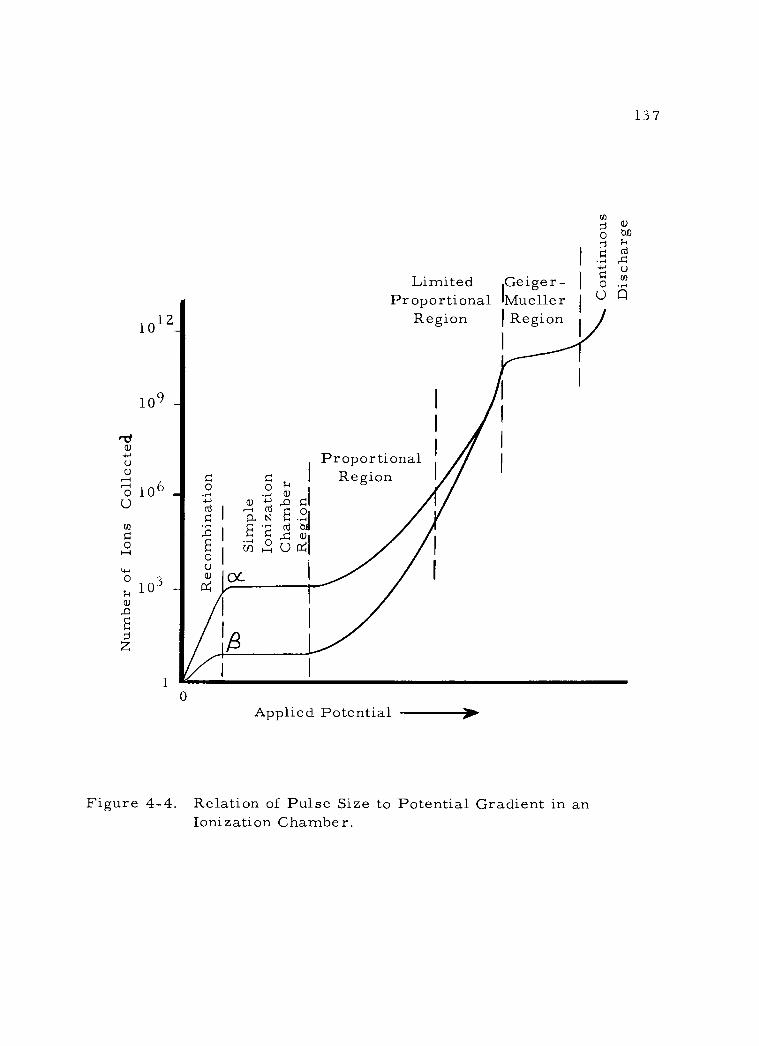
137
101
109
Limited Proportional
Region
Geiger - Mueller Region
co
o
. o
U
a) bo
at .. o u) .--.
n
Proportional I
!
Region á
I
a) 4' II
EN cd bD o áa,°
_ I
Applied Potential
Figure 4 -4. Relation of Pulse Size to Potential Gradient in an Ionization Chamber.
o
.
2 I
N
ó
138
any of these regions by a mere change of potential gradient. Normally
chambers are designed to be operated in a particular region under
specific conditions of internal pressure and potential. Moreover, the
potential gradient needed to define each region is dependent on many
factors, including the filling gas, chamber size, etc.
b. The proportional region: In detectors operating in the pro-
portional region, the number of ions forming an output pulse is very
much greater than the number formed by the initial ionization. Gas
amplification factors ( "A" values) of the order of 103 to 104 are corn-
monly obtained. The amplification factor is primarily dependent on
the composition of the chamber filling gas and the potential gradient.
At a given potential the "A" value is the same for all ionizing events.
Consequently, if an alpha particle traversing the ionization chamber
causes 105 primary ion pairs, with an amplification factor of 103, a
charge of 108 electrons would be collected at the anode. An incident
beta particle, on the other hand, producing only 103 ion pairs, would,
after amplification by the factor of 103, result in a collected charge
of only 106 electrons.
The proportionality observed between the charge collected and
the extent of the initial ionization is the basis for the name of this re-
gion. As in the case of simple ionization chambers, then, it is pos-
sible in the proportional region to differentiate between alpha and beta
139
particles on the basis of pulse size. This is one of the advantages of
operating a detector in this region. Because the amplification factor
in the proportional region is so heavily dependent on the applied poten-
tial, it is necessary to employ highly stable high voltage supplies.
The avalanche of electrons in proportional detectors is collect-
ed on only a portion of the anode wire, usually the tip. Furthermore,
only a small fraction of the gas volume of the ionization chamber is
involved in the formation of ions. These characteristics make for a
very short dead time, i. e. , the interval during which ion pairs
from a previous ionization event are being collected and the chamber
is rendered unresponsive to a new ionizing particle. Ionization cham-
bers operating in the proportional region are thus inactivated for only
5 -50 microseconds following each ionization event.
c. The limited proportional region: The next potential region
is similar to the porportional region in operating characteristics with
one important exception. The extent of gas amplification possible has
an upper limit set by the size of the detector chamber, the form of the
collecting electrode, and the number of gas atoms present. As this
limit is approached, ionization extends essentially throughout the en-
tire chamber involving nearly all of the available gas atoms, and elec-
trons are collected along the entire length of anode wire. At poten-
tials above this limit there is insufficient "ion space" in the chamber
I
140
to accomodate all the ion pairs which theoretically could be formed.
At first, this limits the amplification possible only for highly ionizing
radiation, such as alpha particles.
Let it be assumed, for example, that the total number of ion
pairs that a given chamber can accomodate is limited to 1010 ion pairs,
and an "A" value of 107 is obtained at the potential being used. An in-
cident alpha particle that created 105 primary ion pairs could only be
amplified by a factor of 105 to a maximum of 1010 (instead of 1012) ion
pairs. Under the same conditions, a low E max beta particle initiating
only 102 primary ion pairs would be amplified to a collected charge of
109 electrons. Accordingly, in these circumstances, the proportion-
ality between primary ionization and collected charge is limited, and
the distinction between alpha and beta particles is minimized. This
will be observed by the convergence of the curves for alpha and beta
radiation in Figure 4 -4. For this reason the limited proportional re-
gion is not normally used for detection purposes.
d. The Geiger -Mueller region: At still higher potential gra-
dients the "A" value may reach 108. Now even a weak beta particle
or gamma ray is able to initiate sufficient ion pair formation to com-
pletely fill the available "ion space" in the chamber. Consequently,
the size of the charge collected on the anode is independent of the
number of primary ions produced, and it is no longer possible to
141
distinguish between the various types of radiation. This potential
level is known as the Geiger -Mueller region after the German physi-
cists who first investigated it. Ionization chambers operated in this
potential region are commonly called Geiger - Mueller (G -M) detectors.
Since maximal gas amplification is occurring in this region, the size
of the output pulse from the detector is virtually independent of poten-
tial over a considerable voltage range. This makes possible the utili-
zation of a considerably less stable high voltage supply than required
for proportional detectors with an accompanying reduction in cost.
(1) Dead Time: The employment of a very high amplifica-
tion factor in the Geiger region is not without problems. One of these
is the longer dead time of the chamber. Following the passage of an
ionizing particle through a detector, an electron avalanche occurs
along the entire anode wire. This gives rise to a cylindrical space
charge of positive ions surrounding the anode. The number of such
positive ions per pulse will be one or more orders of magnitude great-
er than in chambers operated in the proportional region. To be dis-
charged, this mass of positive ions must migrate to the cathode wall.
Being much more massive than the electrons, these ions move at a
considerably slower velocity in the electrical field. During this mi-
gration the chamber is unresponsive to any new ionizing particles
passing through it. Thus, the dead time of a detector operated in the
142
Geiger region is from 100 -200 microseconds or more. The impor-
tance of this characteristic in radioactive determinations will be con-
sidered in Chapter 9.
(2) Quenching: Another important problem is that of termi-
nating chamber ionization, which is perpetuated when positive ions
discharge at the cathode wall of a detector. As a positive ion closely
approaches the cathode, it attracts an electron from the wall and be-
comes a neutral atom. This electron, however, will initially be in an
orbit with a higher energy state than the original electron ejected in
ionization. When it falls to the ground state in the atom, the excess
energy then available will be released as electromagnetic radiation.
Some of this radiation will be in the ultraviolet or soft x -ray range.
Such photons are energetic enough to create ion pairs, leading to a
new avalanche of ions. Thus, self -perpetuating ionization would pre-
vail in the chamber, rendering it unresponsive to additional ionizing
particles.
A means of terminating, or "quenching" the discharge event
must be employed. One of the earlier methods utilized some type of
external quench to momentarily reduce the potential in the detecting
chamber. This was accomplished either by a suitable external resis-
tance or an external electronic circuit which lowered the potential
across the electrodes for a sufficiently long period to allow all positive

143
ion discharge and secondary photoelectron production to cease. The
disadvantage of this method was that it was slow and increased the al-
ready long dead time of this type of detector.
More recently, selected gases have been introduced into G -M
detectors to serve as quenching agents. This method is known as in-
ternal quenching, or self -quenching. Two different types of quenching
gases are in common use -- polyatomic organic gases and halogen
gases. The principle involved is that the molecules of the quenching
gas, having a lower ionization potential than the other filling gases,
interact with the positive ions produced by an ionization event in the
detector to prevent continual discharge.
Choosing ethyl alcohol vapor as an example (one of the com-
monest organic gases used), the chain of events in quenching action
may be followed. As they move toward the cathode wall, positive ions
of the inert filling gas (usually argon, helium or neon) collide with al-
cohol molecules. Since the quenching gas has a lower ionization poten-
tial than the inert gas, for example argon, the net result is that the
positive argon ions are discharged into neutral argon atoms, while the
alcohol molecules are ionized. The positive alcohol ions then migrate
to the cathode wall, pick up electrons and become neutral ethyl alcohol
molecules. However, instead of giving up their excitation energy as
electromagnetic radiation, leading to a perpetuated pulse in the tube,

144
the alcohol molecules irreversibly dissociate chemically into degrada-
tion products. This is an effective quenching mechanism, but has the
obvious disadvantage that, since some quenching gas molecules are
destroyed after each ionization event, the life of the detector is finite.
The useful life of such an organic -quenched tube is about 108 pulses.
In halogen - quenched tubes, on the other hand, the dissociated
molecules of the quenching gas readily recombine. In this way,
quenching occurs without irreversible loss of the quenching gas.
Theoretically at least, the useful life of such a G -M detector is infi-
nite. Bromine or chlorine are commonly employed from this purpose.
Unlike the uniform quenching action in organic -filled detectors, the
halogen - quenched G -M tubes may show considerable variation in
quenching efficiency for various portions of the chamber volume. This
limits their use to applications not requiring a high degree of preci-
sion, such as radiation monitoring.
3. Proportional detectors
a. Construction: The operation and characteristics of a corn-
plete proportional counting assembly are discussed in Experiment II
of Part Two of this book. Only the detector itself will be considered
here. Detectors made to operate in the proportional region have taken
many forms. The commercially produced detectors used in
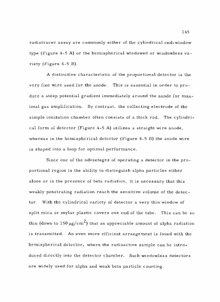
145
radiotracer assay are commonly either of the cylindrical end - window
type (Figure 4 -5 A) or the hemispherical windowed or windowless va-
riety (Figure 4 -5 B).
A distinctive characteristic of the proportional detector is the
very fine wire used for the anode. This is essential in order to pro-
duce a steep potential gradient immediately around the anode for max-
imal gas amplification. By contrast, the collecting electrode of the
simple ionization chamber often consists of a thick rod. The cylindri-
cal form of detector (Figure 4 -5 A) utilizes a straight wire anode,
whereas in the hemispherical detector (Figure 4 -5 B) the anode wire
is shaped into a loop for optimal performance.
Since one of the advantages of operating a detector in the pro-
portional region is the ability to distinguish alpha particles either
alone or in the presence of beta radiation, it is necessary that this
weakly penetrating radiation reach the sensitive volume of the detec-
tor. With the cylindrical variety of detector a very thin window of
split mica or mylar plastic covers one end of the tube. This can be so
thin (down to 150 µg /cm2) that an appreciable amount of alpha radiation
is transmitted. An even more efficient arrangement is found with the
hemispherical detector, where the radioactive sample can be intro-
duced directly into the detector chamber. Such windowless detectors
are widely used for alpha and weak beta particle counting.
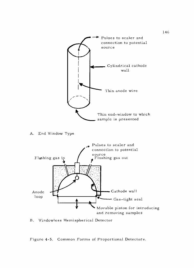
146 ---P" Pulses to scaler and
connection to potential source
A. End Window Type
Flushing gas
Anode loop
Cylindrical cathode wall
Thin anode wire
Thin end - window to which sample is presented
Pulses to scaler and connection to potential source
A
Flushing gas out
Cathode wall -- Gas -tight seal
Movable piston for introducing and removing samples
B. Windowless Hemispherical Detector
Figure 4 -5. Common Forms of Proportional Detectors.
iii
147
With either ultrathin end - window or windowless detectors a
certain amount of air leaks into the counting chamber. Both the oxy-
gen and nitrogen of the air reduce the detection efficiency. The cham-
ber must be purged with a suitable gas before counting is started, and
continually flushed at a lower flow rate during the counting operation.
For this reason, such chambers are often called "gas flow detectors."
The operating potential of the chamber is determined to a large extent
by the gases used for the above purpose. Commonly used are argon,
methane, or a 90 percent argon- 1 0 percent methane mixture known as
P -10 gas.
A proportional detector must be connected to accessory equip-
ment such as a high voltage supply, amplifier, and scaler, in order
for the pulses produced to be properly registered. The functions of
these components are discussed in Experiment II of Part Two.
b. Operating characteristics: When the count rate of a sample
emitting both alpha and beta particles is determined over the voltage
range of a proportional detector and the data are plotted, the results
are as seen in Figure 4-6. This curve should be carefully distinguish-
ed from the plot illustrated in Figure 4 -4, which shows the variation
of charge collected for a single ionizing particle. The characteristic
curve for a proportional detector exhibits two plateaus. The plateau
at the lower potentials represents alpha radiation alone. This is due

148
Beta Plateau
Count Rate
Alpha Threshold
Alpha Plateau
Beta Threshold
Alpha Only
Potential Applied to Proportional Detector --0.
Figure 4 -6. Characteristic Curve for a Proportional Detector.
Alpha Plus Beta
1
0 l l
149
to the fact that at this potential range only the alpha particles, with
their much greater specific ionization, produce pulses large enough
to be detected by the associated circuitry. Not only may the alpha
particles thus be counted apart from accompanying beta radiation at
this potential, but the background radiation count rate is extremely
low -- of the order of a few counts per hour.
As the potential gradient is increased, the amplification fac-
tor becomes greater. Eventually, the primary ions produced by the
most energetic beta particles are amplified sufficiently to produce
pulses large enough to be recorded. This point represents the beta
threshold. Further increase in potential gradient allows even the
pulses from the weaker beta particles to be registered. The beta
plateau has now been reached. In actuality, the count rate here repre-
sents alpha plus beta radiation. The efficiency of the proportional de-
tector for gamma radiation is so low that it is seldom used for gamma
counting.
4. Geiger - Mueller detectors
a. Construction: The operation and characteristics of corn-
plete Geiger - Mueller counting assemblies are described in Experi-
ment I of Part Two of this volume. Only the G -M detector itself will
be discussed here. This detector is the most widely used of all types
150
of radiation detectors. In general construction it does not differ signi-
ficantly from the proportional detectors previously discussed. A G -M
tube conventionally takes the form of a cylindrical cathode about 1 -
1 1/2 inches in diameter by 4 - 8 inches in length. A fine central wire
is suspended from insulation at one or both ends of the tube to act as
the collecting anode. The cylindrical cathode may be of metal or of
glass with an applied metallic film. Sensitivity to gamma rays may be
increased by using a bismuth coating on the inside of the cylinder as a
cathode.
The G -M detector tube is filled with a gas mixture, usually at
a reduced pressure. A readily ionizable, inert gas (argon, helium,
neon) makes up the bulk of the gas filling, while only a small amount
of organic or halogen gas is introduced for quenching effect. Window-
less G -M flow detectors, mostly hemispherical in shape, are similar
to the corresponding proportional detectors in construction. They also
have to be flushed continuously with a special gas mixture made up of
about 99 percent helium and one percent butane, or isobutane.
A broad range of different G -M tube varieties is commercially
available (18). Figure 4 -7 illustrates some of these. The end -win-
dow type (A) is the most widely used for radiotracer assay. It is fun-
damentally the same as the proportional detector shown in Figure 4 -5
A. A variety of end - window materials are used. By employing a
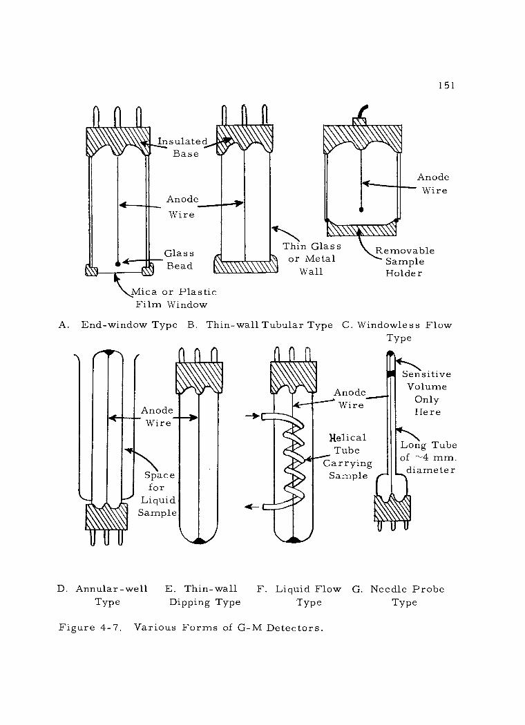
Insulated Base
Anode Wire
Glass Bead
Mica or Plastic Film Window
Thin Glass or Metal
Wall
151
Anode Wire
Removable Sample Holder
A. End - window Type B. Thin -wall Tubular Type C. Windowless Flow Type
Anode Wire
Space for
Liquid Sample
Helical Tube
Carrying Sample
Sensitive Volume
Only Here
Long Tube of ^-4 mm. diameter
D. Annular -well E. Thin -wall F. Liquid Flow G. Needle Probe Type Dipping Type Type Type
Figure 4 -7. Various Forms of G -M Detectors.
152
window of split mica 1-2 mg /cm2 in thickness, it is possible to obtain
the transmission of approximately 2/3 to 3/4 of even the weak beta
particles from C14 into the sensitive volume of the detector (see
Figure 3 -10). Tubes with thicker windows would be utilized primarily
for assay of more energetic beta emitters. Ultrathin windows (less
than 150 µg /cm2) of mylar plastic will transmit even alpha particles,
but such tubes must be operated as flow detectors to counteract the in-
ward diffusion of air. With the windowless flow chamber (C), the max-
imum detection efficiency is obtained, but this detector type allows the
possibility of contamination of the interior of the chamber by radioac-
tive dust or adsorbed vapors.
G -M tubes designed primarily for monitoring purposes (B) are
commonly constructed with thin glass (about 30 mg /cm2) or metal cy-
lindrical walls. This restricts their use to detection of more energe-
tic beta particles or gamma rays. Such tubes are commonly mounted
in probes equipped with adjustable metal "beta shields, " which option-
ally allow gamma rays to be detected to the exculsion of beta radiation.
Tube types D, E, and F were developed for use with radioac-
tive solutions. In the case of type D, the solution is poured into the
annular space around the tube, while type E is actually dipped into a
radioactive solution in a separate container. The design of Figure F
was developed for use with a flow of radioactive liquid. Their
153
necessarily thick, glass walls render these tubes rather inefficient for
beta detection. Since they are gas filled, gamma rays are not readily
detected by them either. In addition, there is the constant problem of
radioactive contamination adhering to the outside of the tube. For
these reasons these three tube types are no longer in common use.
Hidalgo, et al. (13), have described a simplified liquid - sample G -M
detector which is of value for specified radioassays.
The needle probe detector (G) is an example of a highly special-
ized G -M tube, which illustrates the versatility of design possible with
this type of detector. Such tubes have a minute sensitive volume lo-
cated at the tip of the long, thin probe. They are thus useful in pre-
cisely locating radioactive implants or concentrations of radioisotopes
in patients.
Lead shielding around the detector proper is commonly used to
reduce the background radiation count rate. In some circumstances
even this reduced background radiation level cannot be tolerated be-
cause of the very low specific activity of the counting sample. This is
particularly the case in C 14 age- dating measurements. Here, speci-
ally designed "low background counters" may prove necessary. These
typically consist of an "umbrella" of guard G -M detectors surrounding
the sample detector. Anticoincidence circuitry is employed so that
external background radiation, mainly high energy particles, passing
154
through both the guard detectors and the sample detector is not regis-
tered. Only pulses originating in the sample detector alone are regis-
tered. By this means background count rates of only a few counts per
hour are obtainable.
The G -M tube must be connected to some accessory compo-
nents, such as a ratemeter or scaler, so that its output pulses may be
registered. An external high voltage supply is also required. De-
scriptions of these components and details of the operation of the en-
tire counting assembly will be found in Experiment I of Part Two.
b. Operating characteristics: A plot of the count rate from a
fixed radioactive source with increasing potential to the G -M tube is
shown in Figure 4 -8. This should not be confused with the plot illus-
trated in Figure 4 -4, which shows the variation in charge collected
for a single ionizing particle at different detector potentials. The
characteristic curve first shows a sharp rise in counting rate (starting
potential), where only the most energetic beta particles cause the tube
to go into discharge. At the threshold potential this rise levels off
onto a plateau of perhaps 300 volts length. The extent and slope of this
plateau is a measure of the quality of a G -M tube (1 5). At potentials
on the plateau every ionization event occurring in the tube causes a
measurable pulse. Eventually the plateau ends in a second steep rise
in counting rate. Here the potential across the detector electrodes is
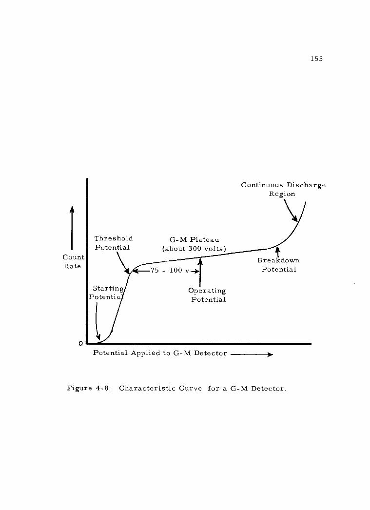
1 Count Rate
Threshold Potential
G -M Plateau (about 300 volts
Starting Potentia
75 - 100 v-0.
155
Continuous Discharge Region
Operating Potential
Breakdown Potential
Potential Applied to G -M Detector )
Figure 4 -8. Characteristic Curve for a G -M Detector.
156
so high that spontaneous discharges can occur in the tube without any
ionization "trigger. " The tube should never be operated in this region
or it may be irreparably damaged. The exact potentials in volts on
the abscissa above are not stated, because these will vary widely with
different tube types and filling gas combinations.
G -M tubes are in general nearly 1 00 percent efficient in detec-
ting alpha and beta particles that reach their sensitive volume, but
only about one percent efficient in detecting gamma rays. The chief
difficulty in the detection of alpha and low Emax beta radiation involves
the extent of absorption occurring in the tube window or wall. Once
inside, the high specific ionization of alpha and beta radiation assures
the initiation of a discharge. The great penetrating power of gamma
rays, which enables them to pass through the walls of a G -M tube
readily, unfortunately allows nearly all these photons to traverse the
filling gas without causing ionization and thus escape detection.
5. Summary of gas ionization detectors
In review, the advantages and disadvantages of detectors oper-
ated in the simple ion chamber, proportional, and Geiger regions will
be compared. Specific examples of detectors used in these three re-
gions that are most commonly employed for radiotracer assay will be
given.

157
The vibrating -reed electrometer is best used to precisely de-
tect low energy beta particles. It is highly stable and requires only a
low chamber potential. A disadvantage of this instrument is that, to
achieve maximum counting efficiency, the sample must be introduced
in a gaseous form into the ion chamber. Under these conditions, how-
ever, it is possible to determine rather large total activities (as much
as one me in a sample). Since no gas amplification occurs in the ion
chamber the weak ionization current produced requires a very high
gain amplification.
Proportional detectors are commonly operated as windowless
flow counters. In this form their high alpha and beta detection effi-
ciency is best used to advantage. In addition, alpha and beta radiation
can be readily distinguished by means of proportional detectors. Pro-
bably their chief advantage is that the very short resolving time inher-
ent in these detectors allows determination of very high count rates
without significant coincidence loss. Their principle disadvantage
lies in the higher gain amplification required, which necessitates more
costly electronic accessory components than for G -M detectors.
The most widely used G -M tube for radiotracer assay is the
thin end - window variety. With this type beta particles are readily de-
tected, with, of course, decreased efficiency for low energy beta ra-
diation. The end - window tube is also generally simpler to operate
158
compared to windowless flow detectors. Due to higher gas amplifica-
tion factors in the G -M chamber, its output pulses need only moderate
amplification, resulting in less costly accessory electronic compo-
nents. Perhaps the greatest disadvantage of the G -M detector is its
long resolving time, which seriously limits the activity of samples
that can be assayed by it. For a comparison of the relative merits of
proportional and G -M detectors the reader is directed to reference
1 4.
Detection in General
BIBLIOGRAPHY
1. Bleuler, Ernst and George J. Goldsmith. Experimental nucleon- ics. New York, Holt, Rinehart and Winston, 1952. 393 p.
2. Bruner, H. D. and Jesse D. Perkinson, Jr. A comparison of iodine -131 counting methods. Nucleonics 10(10) :57 -61 . 1952.
3. Christman, David R. Choosing a method for counting soft betas. Nucleonics 1 9(5):51 -55. 1 961 .
4. Jordan, W. H. Detection of nuclear particles. Annual Review of Nuclear Science 1:207 -244. 1952.
5. Nokes, M. C. Radioactivity measuring instruments. New York, Philosophical Library, 1958. 75 p.
6. Pearson, F. J. and R. R. Osborne. Practical nucleonics. London, E. & F. N. Spon, Ltd. , 1 960. 208 p.
7. Price, William J. Nuclear radiation detection. New York, McGraw -Hill, 1 958. 382 p.
159
8. Sharpe, J. Nuclear radiation measurement. New York, Simmons-Boardman, 1 960. 71 p.
9. Snell, Arthur H. (ed. ). Nuclear instruments and their uses. vol. I. New York, John Wiley, 1962. 494 p.
10. Washtell, C. C. H. An introduction to radiation counters and detectors. New York, Philosophical Library, 1960. 115 p.
11. Wolfgang, Richard and C. F. Mackay. New proportional counters for gases and vapors. Nucleonics 1 6(1 0):69 -73. 1 958.
Gas Ionization Detection
1 2. Brownell, Gordon L. and Helen S. Lockhart. CO?? ion- chamber techniques for radiocarbon measurement. Nucleonics 1 0(2): 26 -32. 1952.
1 3. Hidalgo, J. V. , S. B. Nadler and R. T. Niesets. A simplified liquid - sample geiger counter. Nucleonics 11(2):66-67. 1 953.
14. Proportional vs. Geiger counters. Picker Scintillator (issued by Picker X -Ray Corp. ) 4:1 -4. June 10, 1 960.
15. Reddis, J. S. and Wm. C. Roesch. Two better ways to deter- mine Geiger - Mueller -tube age. Nucleonics 14(7):30 -32. 1956.
1 6. Springell, P. H. Ionization current measurement of aqueous solutions containing C14. The International Journal of Applied Radiation and Isotopes 9:88 -93. 1 960.
1 7. Tolbert, B. M. Ionization chamber assay of radioactive gases. 1956. 47 p. (University of California Radiation Laboratory. UCRL- 3499).
1 8. Van Duuren, K. , A. J. M. Jaspers and J. Hermsen. G -M counters. Nucleonics 1 7(6) :86 -94. 1 959.
CHAPTER 5 - MEASUREMENT OF RADIOACTIVITY BY THE EXTERNAL -SAMPLE (SOLID) SCINTILLATION METHOD
A. Basic Facets of the Scintillation Phenomenon
160
Historically the scintillation phenomenon was in common use
early in this century as a means of detecting alpha particles. Because
the method involved the tedious visual observation and recording of
faint scintillations, it fell into disuse with the advent of gas ionization
detectors. The development of suitable photomultiplier tubes during
World War II, which permitted electronic detection and recording of
individual scintillation events, brought a resurgance of interest in the
scintillation method. Since that time a very rapid expansion of scintil-
lation detector types and applications has occurred.
In the radiation detectors described in the previous chapter,
the detection process involved the collection of the ions produced as a
result of the interaction of radiation with gas in an enclosed chamber.
Scintillation detection, on the contrary, is based on the interaction of
radiation with substances known as fluors (solid or liquid). Excitation
of the electrons in the fluor leads to the subsequent emission of a flash
of light (scintillation). An adjacent photomultiplier tube converts such
photons into a pulse whose magnitude is proportional to the energy
lost by the incident radiation in the excitation of the fluor. Thus

161
scintillation detection is proportional in nature and, when used with a
pulse height analyzer, allows determination of the energy spectrum of
the incident radiation. Comprehensive discussions of the scintillation
mechanism and its application to radiation detectors are found in the
volumes by Curran (4), Birks (2), and Krebs (10).
It is difficult to arrive at a consistent classification of scintil-
lation detectors. The fluor substances may be grouped into two broad
categories: inorganic (ionic) and organic fluors. Inorganic fluors are
normally used in the form of single, large crystals. Organic fluors,
by contrast, may be employed as single crystals, as a compact mass
of fine crystals, impregnated in a plastic polymer, or dissolved in an
organic solvent (liquid fluor). The scintillation process in organic and
inorganic fluors differs somewhat. In organic fluors scintillation is
primarily a molecular phenomenon and is marked by a ready transfer
of excitation energy from molecule to molecule, especially in the case
of dilute liquid fluors. Scintillation in inorganic fluors, on the other
hand, results largely from the electronic structure of the crystals and
the presence of specific activating "impurities" in the crystalline lat-
tice.
Scintillation detectors may also be categorized on the basis of
the relation of the sample and the fluor. In the case of external -sam-
ple scintillation detectors, radiation from an external source interacts

162
with a fluor (usually a single crystal or plastic block), which is coupled
to a photomultiplier. If the radioactive sample and the fluor are in in-
timate contact (dissolved in a common solvent, or one suspended in a
solution of the other) and placed adjacent to one or more photomulti-
pliers, an internal - sample scintillation detector results. This ar-
rangement is most commonly referred to as a liquid scintillation de-
tector. In this text scintillation detectors will be somewhat arbitrarily
divided into external - sample (employing solid fluors) and internal -
sample (usually involving liquid fluors) detectors. The remainder of
this chapter will describe the former type, while the next chapter will
discuss internal - sample detectors.
B. External - sample (Solid) Scintillation Detectors
1. Mechanism of external - sample scintillation detection.
Scintillation detection involves a series of energy conversions
from the initial interaction with the fluor until an output pulse leaves
the photomultiplier. These steps will be discussed below in their nor-
mal sequence, primarily emphasizing gamma ray detection by ionic
crystal fluors. Figure 5 -1 will aid the reader in visualizing the vari-
ous portions of a typical scintillation detector in relation to these
energy conversion steps. Detailed information concerning the various
detector components themselves will be considered later in the chapter.

163
Gamma Ray
Scintillation
Dynodes Photomulti plier Tube
Fluor Crystal Na I(T1)
Reflector Housing
Photoelectrons
Photocathode
Figure 5 -1. Diagram of a Typical Solid Fluor External- Sample Scintillation Detector.
4/
164
a. Energy conversion in the fluor crystal: As a gamma ray
traverses a fluor crystal it may dissipate some of its energy
(see Chapter 3). The extent of this energy dissipation is directly re-
lated to the density and thickness of the fluor substance. It will be re-
called that gamma rays commonly interact with matter by means of
three distinct processes -- pair production, Compton effect, and the
photoelectric process. In each case electrons are ejected, which in
turn are able to produce excitation or ionization of adjacent portions
of the fluor crystal. It is this secondary excitation of the fluor that is
particularly important here. The total amount of excitation produced
in a fluor is directly related to the amount of energy dissipated by a
traversing gamma ray.
Excitation of a fluor occurs when one of its orbital electrons is
raised to a higher energy level as a result of energy dissipation by a
passing charged particle. Immediate de- excitation occurs as the elec-
tron returns to its ground state and the excitation energy is emitted as
a photon. It is at this point that a difference between the scintillation
process in organic and inorganic crystals exists. In organic crystals
the events just described are distinctly molecular phenomena, while in
inorganic crystals the excitation energy migrates to an activator cen-
ter where de- excitation results in photon emission. Thus, ionic fluors
normally require the presence of some activation substance for
165
maximum light production efficiency, while organic fluors do not. In
fact, organic fluors must be scrupulously purified.
Fluor substances are selected on the basis of emitting a high
proportion of excitation energy as visible light (scintillations) with a
o wave length near 4100 A. The number of such photons produced is
directly related to the amount of excitation energy resulting from a
given gamma ray.
b. Energy conversion in the Photomultiplier: The photons of
visible light pass through the transparent fluor substance and out
through a clear window to impinge on an adjacent photocathode. The
typical photocathode is composed of a thin photosensitive layer (com-
monly Cs -Sb) on the inner surface of the end of the photomultiplier
tube. Here impinging photons in the visible light range are absorbed,
with a consequent emission of photoelectrons. The number of photo-
electrons ejected is less than, but directly related to, the number of
incident photons. Such a burst of photoelectrons resulting from a sin-
gle gamma ray interaction is still far too weak to be directly regis-
tered.
Amplification occurs by means of a series of electrodes, called
dynodes, spaced along the length of the photomultiplier tube. Each dy-
node is maintained at a higher potential (usually about 100 - 200 volts
higher) than the preceding one. By means of this arrangement,
166
photoelectrons ejected from the photocathode are accelerated toward
the first dynode. Striking the dynode surface, they bring about the
secondary emission of a larger number of electrons. This new burst
of electrons is attracted by the potential gradient to the second dynode
in the series, where a still larger number of electrons is dislodged.
This electron multiplying process continues at each dynode until at
last the collecting anode is struck by 105 - 106 electrons for each ori-
ginal photoelectron ejected from the photocathode. Thus, the magni-
tude of the output pulse from the photomultiplier is directly related to
the quantity of energy dissipated by the incident gamma photon in the
fluor.
c. Proportionality of energy conversion: In order to present
a quantitative example of the energy conversions involved in scintilla-
tion detection, the results of the interaction of a single 1. 17 Mev gam-
ma ray from Co" with a thallium- activated sodium iodide crystal
[ NaI (T1) ] will be traced.
(1) If 20 percent of the energy of the gamma ray is transferred
to a fluor crystal, and if it is assumed that each excitation
event requires an average of ten ev, then approximately
23, 400 excitations could result from this gamma photon.
(2) Assuming that only 5% of the excitation events result in the
production of photons of visible light which are seen by the
167
adjacent photocathode, this would mean that about 1, 170
photons would reach the photocathode.
(3) This number of photons striking a photocathode with a
conversion efficiency of ten percent would eject approxi-
mately 117 photoelectrons.
(4) The successive dynodes of a photomultiplier operated at an
overall gain of 106 could then amplify this quantity of
photoelectrons so that 1. 17 x 108 electrons would be col-
lected at the photomultiplier anode, or a charge of approxi-
mately 2 x 10 -11 coulombs.
(5) This charge could then be transformed by a pre -amplifier
circuit with a capacitance of 30 pp.f into an output pulse of
about 0. 6 volts. A pulse of this size would be capable of
directly operating the detecting circuitry of a scaler.
Cobalt -60 emits two gamma rays per disintegration. The
other gamma ray has an energy of 1.33 Mev. Following the same cal-
culations as above, this 1.33 Mev gamma would result in an output
pulse of about 0. 7 volts from the detector. It should be appreciated
that such energy calculations are based on several variables and are
only very crude approximations of true values. The importance of
these calculations is to indicate that the size of the photomultiplier out-
put pulse is directly proportional to the amount of energy dissipated in
1 68
the fluor by the incident gamma photon. This relationship makes pos-
sible the determination of gamma ray energy when a pulse height
analyzer is used with the detector, of which more will be said below.
d. Other advantages: In addition to the possibility of deter-
mining gamma ray energies, three other advantages of this type of de-
tector should be indicated. First, because the photons produced in the
fluor have decay times of millimicroseconds to microseconds, very
high counting rates can be recorded by scintillation counters with no
coincidence loss. Secondly, in the example above of Co60, the 0.314
Mev beta particles also emitted would not be detected appreciably.
This is because the NaI (Ti) crystal is enclosed in an aluminum con-
tainer, which absorbs most of the beta radiation. In addition, this
fluor is not an efficient beta detector. Thus, solid fluors offer an ex-
clusive means of detecting gamma rays. Thirdly, the higher densi-
ties of solid fluors, as compared to gases or liquids, result in greater
gamma ray stopping power and consequent increased detection effi-
ciency.
e. Photomultiplier thermal noise: Unfortunately, scintilla-
tion detection is not without complications. The high potential applied
between the photocathode and the dynodes in the photomultiplier also
gives rise to thermionic emission. A certain number of photoelec-
trons will thus be emitted, even when no light falls on the photocathode.
1 69
These produce small sized pulses known as "thermal noise ", or "dark
current. " Since the magnitude of thermal noise is dependent on the
potential applied to the photomultiplier, this factor becomes important
in determining the optimal operating potential of a scintillation detec-
tor (Experiment III).
Thermal noise may be minimized in several ways. Certain
new photomultipliers have been designed with considerably reduced
thermal noise levels. A simple pulse height discriminator circuit will
bar the detection of the weaker noise pulses, while the larger gamma
pulses are counted. In cases where the sample pulses do not greatly
exceed the size of the noise pulses, other means must be employed.
This is the problem in low energy beta detection using liquid fluors,
as will be discussed later. Suffice it to say that cooling the photomul-
tipliers (9) and /or using coincidence circuitry virtually eliminates the
problem of thermal noise.
f. Gamma ray spectrometry: In determining the energy levels
of gamma rays from a given nuclide (gamma spectrum), it would
be highly desirable to have each incident gamma ray dissipate all its
energy in the fluor by photoelectric absorption. In this case a line
spectrum, as shown in Figure 5 -2A, would be obtained. However,
partial energy dissipation by Compton interaction also occurs. Since
any fraction of the gamma ray energy can be thus dissipated, a
170
continuous spectrum (the "Compton smear ") is produced. Interaction
by pair production also complicates the spectrum, as well as a num-
ber of other factors. Figure 5 -2 B shows a typical gamma ray spec-
trum for Co60. These various modes of gamma interaction do not af-
fect simple gamma pulse counting, but do make interpretation of gam-
ma spectra difficult. A more detailed discussion of gamma spectro-
metry is beyond the scope of this volume. For further information
the reader is directed to the concise booklet published by the Baird -
Atomic Company (1).
2. Components of external sample scintillation detectors
a. Detector housing: The entire scintillation detector is
housed in a light- tight, thin metal cylinder. This gives mechanical
protection to all components, as well as preventing stray light from
reaching the photocathode while it is in operation. Protection against
the effect of exterior magnetic fluxes on the photomultiplier is afforded
by a Mu -metal shield. Where directional sensitivity is desired, a lead
collimator may be fitted over the scintillation crystal. Incident radia-
tion must pass through the light -tight enclosure around the fluor to in-
teract and be detected. In the case of gamma rays, the thin aluminum
"can" of about 0. 03" presents no absorption problem. However, for
crystal fluors used to detect alpha or beta particles, ultrathin entrance
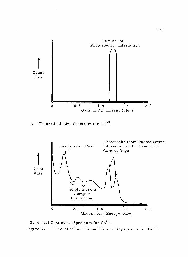
1 Count Rate
Results of Photoelectric Interaction
171
0 0.5 1.0 1.5 Gamma Ray Energy (Mev)
A. Theoretical Line Spectrum for Co 60.
1 Count Rate
Backscatter Peak
2. 0
Photopeaks from Photoelectric Interaction of 1. 17 and 1.33 Gamma Rays
Photons from Compton
Interaction
0 0.5 1.0 1.5 Gamma Ray Energy (Mev)
B. Actual Continuous Spectrum for Co 60.
2. 0
Figure 5 -2. Theoretical and Actual Gamma Ray Spectra for Co60
11\

172
windows of aluminum foil or aluminized Mylar film must be employed.
b. Fluor crystals: Scintillation crystals are commonly, but
erroneously, referred to as phosphors. These crystals are used for
radiation detection because they show very short -lived fluorescence
following energy absorption, and are thus technically fluors. If they
were true phosphors, producing long lasting phosphorescence, they
would be quite unsuitable for this purpose.
As has been previously mentioned the commonly used fluors
can be divided into two categories -- inorganic (ionic) crystals and or-
ganic crystals. The fluorescent property of the inorganic crystals is
lost when the crystals are dissolved, but the organic fluors may be
used either in crystalline form or dissolved. When dissolved in vari-
ous organic solvents, they form liquid fluors, which will be further
discussed in the next chapter. Organic fluors such as anthracene or
p- terphenyl have also been used to impregnate polystyrene or poly -
vinyltoluene. In this form they are called plastic fluors and have the
advantage of being formed or machined into a wide variety of shapes
and sizes (3, 8). Plastic fluors give poor energy resolution and, thus,
are not useful in spectrometry. Table 5-1 lists the properties of some
common crystalline fluors. In addition, two reviews by Swank (15,
16) provide more detailed information on fluor characteristics.
Since the photoelectric absorption coefficient varies approxi-
mately as the fifth power of the atomic number of the absorber, the
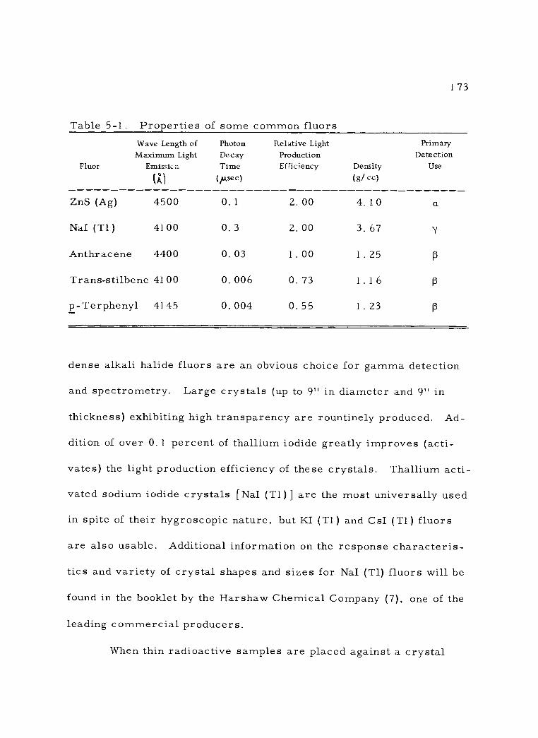
1 73
Table 5-1. Properties of some common fluors Wave Length of Maximum Light
Fluor Emission
(n
Photon Decay Time
(, &sec)
Relative Light Production Efficiency Density
(g/ cc)
Primary Detection
Use
ZnS (Ag) 4500 0. 1 2. 00 4. 10 a
NaI (T1) 41 00 0. 3 2. 00 3. 67
Anthracene 4400 0.03 1.00 1.25 ß
Trans-stilbene 4100 0. 006 0. 73 1 . 1 6 ß
p-Terphenyl 4145 0.004 0.55 1.23 ß
dense alkali halide fluors are an obvious choice for gamma detection
and spectrometry. Large crystals (up to 9" in diameter and 9" in
thickness) exhibiting high transparency are rountinely produced. Ad-
dition of over 0. 1 percent of thallium iodide greatly improves (acti-
vates) the light production efficiency of these crystals. Thallium acti-
vated sodium iodide crystals [NaI (T1) ] are the most universally used
in spite of their hygroscopic nature, but KI (T1) and CsI (T1) fluors
are also usable. Additional information on the response characteris-
tics and variety of crystal shapes and sizes for NaI (T1) fluors will be
found in the booklet by the Harshaw Chemical Company (7), one of the
leading commercial producers.
When thin radioactive samples are placed against a crystal
y
174
fluor for assay, a maximum of 50 percent of the radiation is emitted
in the direction of the detector (2 1r geometry). In an effort to increase
detection efficiency, fluors have been prepared with a "well" drilled
into the crystal. Assay samples may then be placed essentially within
the crystal, so that a much greater proportion of the radiation emitted
may be detected. Such a well crystal is particularly suited for direct
assay of liquid samples (6, 12, and Experiments C and D, Part Three),
homogenized tissue, or ashed specimens (Experiment E, Part Three).
NaI (Tl) crystals with well sizes capable of accomodating fluid sam-
ples up to 25 ml. are commonly available. Plastic fluors can be fabri-
cated with very much larger well sizes.
Organic fluors in the form of single crystals are less com-
monly employed in radiotracer assay. Because of their low densities,
they are considerably less efficient for detecting gamma rays than the
alkali halide crystals. Although they are intrinsically quite efficient
for beta detection, the G -M detector is as efficient, and considerably
less costly. The organic crystal detectors, however, do have the ad-
vantage of an energy- dependent response, and so find limited use in
beta ray spectrometry. Their temperature dependence has been in-
vestigated by Liebson (1 1 ).
c. Photocoupling: In order to direct the maximum number of
photons from the scintillation crystal to the photocathode, certain
1 75
optical features must be included in the detector. The side of the
crystal housing facing the photocathode is formed by an optical window
of clear glass or quartz. All other surfaces of the crystal are covered
with a light reflecting layer, commonly Al2O3 or aluminum foil. Good
optical contact between the crystal and the photomultiplier tube is ob-
tained by means of a transparent viscous medium, such as Dow -
Corning "200" silicone fluid. In applications where it is desirable to
have the scintillation crystal in probe form to reach less accessible
positions, a "light pipe" of lucite or quartz is used to connect it with
the photomultiplier tube.
d. Photomultiplier tubes: A photomultiplier tube consists of
a photosensitive cathode, a series of dynodes maintained at increas-
ingly positive potentials to the cathode, and an electron collecting
anode, all sealed in a glass envelope. Both the photocathode and the
dynodes have sensitive surfaces which are capable of emitting elec-
trons when struck by incident photons or electrons. It is this property
of secondary emission that allows electron multiplication to occur
through the dynode series, as has been previously described. Photo -
multiplier tubes for scintillation detection are principally available
from four manufacturers at present -- Radio Corporation of America
(RCA), DuMont, CBS Labs, and Electrical and Musical Industries,
Ltd. (EMI). The review by Sharpe and Thomson (13) describes

176
construction and operating features of all commonly used photomulti-
plier tubes.
A variety of photocathode materials have been used in the past,
but antimony- cesium or silver- magnesium alloys are currently the
most widely employed (14). This is due both to the relatively high light
sensitivity (40 - 60 p.a /lumen) and quantum efficiency, or the ratio of
photoelectrons ejected to incident photons, (10 - 20 percent) of these
alloys, and to the fact that their spectral sensitivity matches the emis-
sion spectra of the most commonly used fluors. Figure 5 -3 graphi-
cally illustrates this latter relationship in the case of NaI (T1) and
anthracene fluors. Although photocathodes over 4" in diameter are
available, the larger sizes commonly lack uniformity of response.
When large size crystals or fluor solutions are employed, a number
of photomultipliers can be arranged to detect the scintillations.
Two principal types of construction are used for the dynode
series in photomultipliers. Tubes of American manufacture commonly
contain curved dynodes arranged so that an electrostatic field focuses
the electron burst from one dynode to another. This is diagrammati-
cally shown in Figure 5 -1. The EMI tubes use flat dynodes arranged
like a series of venetian blinds. In either case the total amplification
depends on the number of dynode stages and the potential applied be-
tween successive stages. From 6 to 14 dynodes may be included and
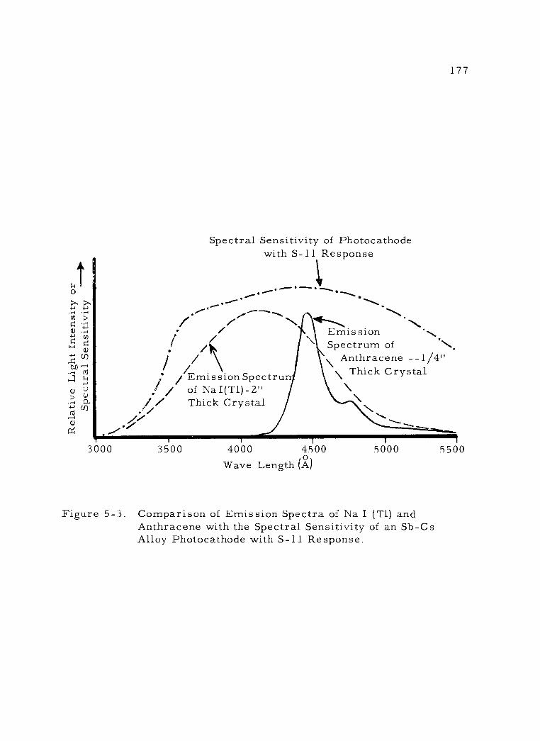
Relative
-I-, .. -1-, . a)
Cf) 1-4 ! , o,
4 0/Emission Spectru 4-, / of NaI(T1) -2"
// / Thick Crystal á ,>
Spectral Sensitivity of Photocathode with S -11 Response
. ---". ' 3000 3500
Emission
177
Spectrum of Anthracene -1/4" 1 /4"
Thick Crystal
4000 4500 0
Wave Length (X)
5000
Figure 5 -3. Comparison of Emission Spectra of Na I (Ti) and Anthracene with the Spectral Sensitivity of an Sb -Cs Alloy Photocathode with S -11 Response.
5500
. s
/ / / ' / '
n:
178
the potential applied in approximately equal steps of 100 -150 volts.
Thus, an overall potential gradient of up to nearly 3000 volts may be
required, depending on the specific photomultiplier used. The stabi-
lity of the high voltage supply is essential in view of the direct rela-
tion between total amplification and dynode potential. Although gains
of 2 to 3 x 10⁶ are most common, with higher voltages and larger
numbers of dynodes, overall gains of 107 - 108 are possible.
e. Preamplifier: This component is not strictly a part of the
detector, but is usually attached directly to the above components,
often in the same housing. Its function is to amplify the small output
pulses from the photomultiplier sufficiently so that they will not be
lost in traversing the cable to the scaler.
Other components are needed to form a complete scintillation
counting assembly. These include a high voltage supply, scaling unit,
mechanical register, and timer, all of which may be combined into one
unit - a scaler. If spectrometry is to be done, a linear amplifier and
pulse height analyzer will also be required. These components and
their functions will be described in Experiment III, Part Two.
3. Operating characteristics of external- sample scintillation detector s
The determination of the optimal operating conditions for scin-
tillation counters involves two parameters -- the potential applied to
179
the photomultiplier and the gain of the preamplifier or amplifier. In
contrast, such determination for G -M counters involves only the po-
tential applied across the G -M detector electrodes.
a. Effect of photomultiplier potential: At a fixed gain setting,
a series of activity determinations made at successively higher photo -
multiplier potentials will yield data which may be plotted as seen for
the solid line curve in Figure 5 -4. This curve shows the rapid rise
in counting rate at lower potentials, the nearly flat plateau region of
essentially constant counting rate with increasing potential, and final-
ly the second region of rising count rate that superficially appears to
resemble the characteristic G -M plateau curve (Figure 4 -8). Actu-
ally, the two curves are completely unrelated. The plateau on the
scintillation counter curve represents potentials at which virtually all
the photons produced in the fluor are being detected. Engstrom and
Weaver (5) have thoroughly discussed the significance of the scintilla-
tion plateau.
The counting rate from total background radiation and that due
to thermal noise in the photomultiplier alone are also seen in Figure
5 -4. It is evident that the rapidly rising thermal noise level at the
higher voltages is primarily responsible for the increase in total
counting rate of the "background" at the end of the plateau. This being
the case, it is best to operate the scintillation detector at the lowest
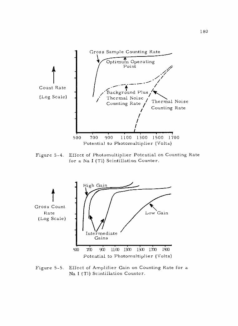
180
fi Count Rate
(Log Scale)
Gross Sample Counting Rate
Optimu Operating Point
/'Background Plus/ Thermal Noise Counting Rate Thermal Noise
Counting Rate
500 700 900 1100 1300 1500 1700 Potential to Photomultiplier (Volts)
Figure 5 -4. Effect of Photomultiplier Potential on Counting Rate for a Na I (Tl) Scintillation Counter.
t Gross Count
Rate (Log Scale)
High Gain
Low Gain
\/ Intermediate Gains
500 rh 900 1100 1300 1500 1700 1900
Potential to Photomultiplier (Volts)
Figure 5 -5. Effect of Amplifier Gain on Counting Rate for a Na I (T1) Scintillation Counter.
.
/ i /
. (
.
.1
i' / /

181
possible potential on the plateau. The optimal operating potential is
chosen on statistical grounds as that potential where the ratio of the
square of the sample count rate to the background count rate is at max-
imum (S2 /B = max. ). Since the plateau curves for different gamma
emitting nuclides vary somewhat, the optimal operating potential must
be determined individually for each isotope used.
b. Effect of amplifier gain: The effect of different amplifier
gain settings on the scintillation counter plateau curve is seen in Fi-
gure 5 -5. It will be found, in general, that increased amplifier gain
results in shortened plateau length, increased counting rate, and de-
creased plateau slope. Since the effects on counting rate of photomul-
tiplier potential and preamplifier gain are somewhat similar, but ther-
mal noise is directly related to photomultiplier potential, it is advis-
able to operate a scintillation counter at the lowest possible potential
and to increase the preamplifier gain as required to compensate.
c. Gamma energy dependence of detection efficiency: The
gamma detection efficiency of a NaI (T1) scintillation counter is strong-
ly dependent on the energy of the incident gamma rays. This relation-
ship is seen in Figure 5 -6. Such variation in detection efficiency for
different isotopes must be considered in experimental design (see
Chapter 10). This energy dependence is explained by considering the
nature of the competing effect of the three gamma interaction
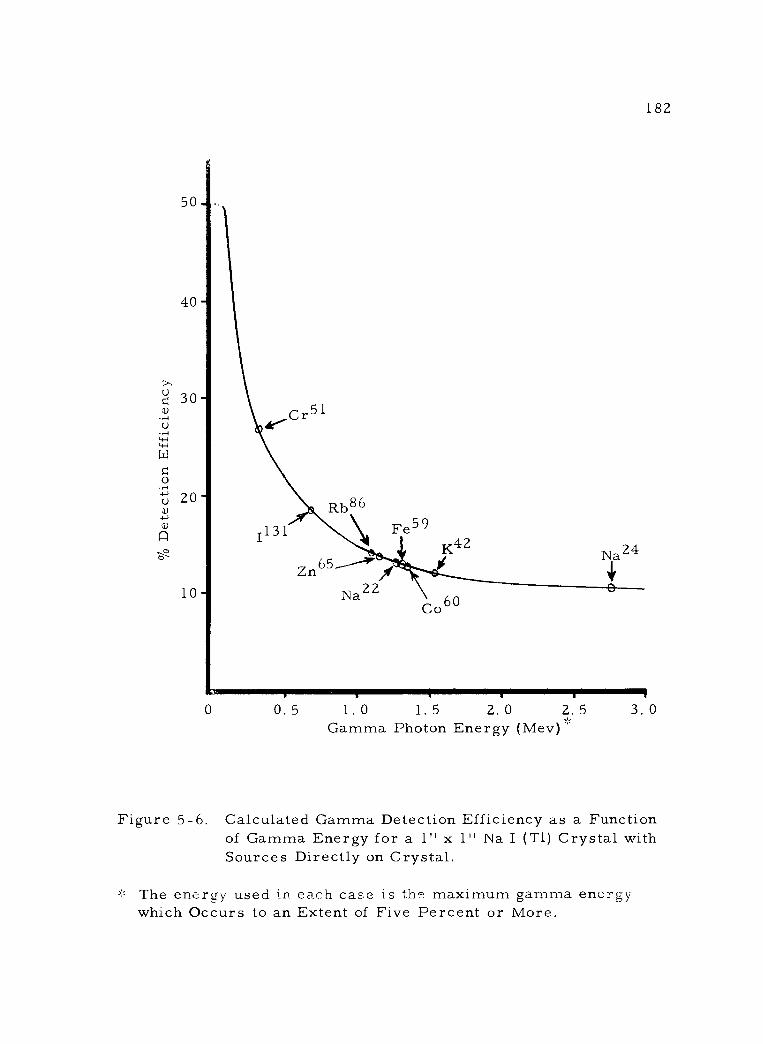
% D
etection Efficiency
50
40
30
20 Rb86
1131 \, Fe59 K42 Na24
Zn65/ 10 Na22 60 Co
182
0 0.5 1.0 1.5 2.0 2.5 Gamma Photon Energy (Mev)
3. 0
Figure 5 -6. Calculated Gamma Detection Efficiency as a Function of Gamma Energy for a 1" x 1" Na I (T1) Crystal with Sources Directly on Crystal.
The energy used in each case is the maximum gamma energy which Occurs to an Extent of Five Percent or More.

1 83
processes (see Chapter 3). It should be clear that use of larger scin-
tillation crystals would improve the detection efficiency at higher gam-
ma energies, since there would be an increased probability of inter-
action as the gamma rays traversed the crystal. Of course, use of
larger crystals also results in increased background counting rate.
The background counting rate can be reduced by the use of a spectro-
meter, although at the cost of reduced counting efficiency for the sam-
ple activity.
BIBLIOGRAPHY
1. Baird -Atomic, Inc. Scintillation spectrometry. Cambridge, Mass. , 1 960. 63 p.
2. Birks, John B. Scintillation counters. New York, McGraw -Hill, 1953. 148 p.
3. Buck, Warren L. and Robert K. Swank. Preparation and perfor- mance of efficient plastic scintillators. Nucleonics 11 (11 ):48- 52. 1 953.
4. Curran, S. C. Luminescence and the scintillation counter. New York, Academic Press, 1953. 219 p.
5. Engstrom, Ralph W. and J. L. Weaver. Are plateaus significant in scintillation counting? Nucleonics 17(2):70 -74. 1959.
6. Haigh, C. P. Gamma -ray scintillation counter for weak radio- active solutions. Nucleonics 1 2(1 ):34 -39. 1954
7. Harshaw Chemical Company. Harshaw scintillation phosphors. Rev. ed. Cleveland, 1 960. 44 p.

1 84
8. Hine, Gerald J. and John A. Cardarelli. Conical plastic scintil- lators show total gamma absorption. Nucleonics 1 8(9):92- 1 00. 1 960.
9. Hinard, Frank E. Temperature dependence of photomultiplier gain. Nucleonics 15(4):92 -97. 1 957.
10. Krebs, A. T. Early history of the scintillation counter. Science 1 22:1 7 -1 8. 1 955.
11. Liebson, S. H. Temperature effects in organic fluors. Nucleo- nics 1 0(7):41 -45. 1 952.
12. Maclntyre, William J. and James H. Christie. A well scintilla- tion counter for improved volume efficiency. The Journal of Laboratory and Clinical Medicine 50 :653 -656. 1 957.
13. Sharpe, J. and E. E. Thomson. Photomultiplier tubes and scin- tillation counters. In: Proceedings of the Second United Nations International Conference on the Peaceful Uses of Atomic Energy, Geneva, 1958. vol. 10. Nuclear physics and instrumentation. Geneva, United Nations, 1 958. p. 311 - 324.
14. Sommer, A. H. New photoemissive cathodes of high sensitivity. The Review of Scientific Instruments 26:725 -726. 1955.
15. Swank, Robert K. Recent advances in theory of scintillation phosphors. Nucleonics 1 2(3) :1 4 -1 9. 1 954.
16. Swank, Robert W. Characteristics of scintillators. Annual Review of Nuclear Science 4:111 -140. 1 954.
185
CHAPTER 6 - MEASUREMENT OF RADIOACTIVITY BY THE INTERNAL - SAMPLE (LIQUID) SCINTILLATION METHOD
Liquid scintillation counting owes its origin to the indepen-
dent discovery by Reynolds (75) and Kallman (51) in 1 950 that certain
organic solutions fluoresce noticeably when bombarded with high en-
ergy radiation. This fluorescence can then be readily magnified with
a photomultiplier and measured as an electrical pulse, as in the case
of solid fluor detectors. Liquid fluors, however, offer a significant
advantage over solid fluors. The radioactive sample and the fluor are
mixed intimately in a homogeneous medium (internal -sample), either
dissolved or suspended in a suitable solvent. With this system, vir-
tually 4Tr detection geometry is realized. Moreover, the detection
sensitivity is such that low energy beta emitters can be assayed with
quite respectable efficiency. It is this latter application that has been
most widely exploited and that will be emphasized in this chapter.
Liquid scintillation detectors have come into general usage
in radiotracer laboratories in only the most recent years. This is
due in part to the expense of the complete counting assemblies that
are commercially available. This expense is due largely to the far
greater complexity of the electronic circuitry involved in the liquid
scintillation counting assembly, as compared to those used with other
detector types.
186
Another reason, perhaps equally important, for the hesitancy
of many investigators in using the liquid scintillation detection method
is the present state of the literature on the subject. Articles published
on the methodology itself are relatively few in number, and are scat-
tered through a wide variety of journals. Several symposia have dealt
largely or entirely with liquid scintillation detection and their publish-
ed proceedings have formed the core of the readily available literature
(11, 24, 79). At present, no comprehensive monograph on the subject
has been produced. A number of brief reviews of the detection method
may be found (5, 10, 49, 72, 80), in addition to which the more thor-
ough coverages by Davidson and Feigelson (25), Hayes (42 -43) and
Kobayashi (60) are to be highly recommended. Various instrument
manufacturers, notably Packard, Nuclear -Chicago, and Tracerlab
include brief descriptions of the methodology in their instrument man-
uals. They also provide a series of technical bulletin covering various
phases of liquid scintillation detection (21, 23, 45, 91). In view of this
situation, the major purpose of this present chapter and the portion of
Chapter 8 devoted to the preparation of samples for liquid scintillation
detection is to provide a fundamental, though brief, survey of liquid
scintillation methodology and a comprehensive list of references to its
literature.
A. Mechanism of Internal - Sample Scintillation Detection
187
The overall sequence in liquid scintillation detection might ap-
pear superficially to be identical with that described for external -
sample scintillation detection in the previous chapter. Fluor mole-
cules are directly or indirectly excited by ionizing radiation resulting
in the emission of photons. These in turn interact with the photoca-
thode of a photomultiplier to yield photoelectrons from the photocathode
surface. The photoelectrons pass through a dynode series and result
in the production of a greatly amplified electron pulse at the photomul-
tiplier anode. However, a basic difference between the two detection
sequences does exist. It lies in the mechanism of energy transfer
from radiation to fluor. This mechanism will be briefly elaborated in
this chapter. For a more detailed discussion of the mechanism of en-
ergy transfer in fluor solutions the reader is directed to the papers by
Birks (24, p. 12 -36), Furst and Kallman (11, p. 3 -22, 28 -29, 52 -54),
Hayes (39), Reynolds (76), and Swank and Buck (90).
1. Energy conversion steps in the fluor solution.
In liquid scintillation detection a small amount of the fluor sub-
stance (the solute) is typically dissolved in a much larger quantity of an
organic solvent to form the fluor solution. The radioisotope sample
188
may be either dissolved or suspended in this solution. Due to the low
concentration of fluor in the solvent (usually less than one percent),
the energy of the beta radiation is not directly transferred to the fluor
molecules to any extent.
The kinetic energy of the primary ionizing particle is prima-
rily transferred to the more abundant solvent molecules, which are
usually of an aromatic hydrocarbon, such as toluene. As a result,
the solvent molecules may be ionized, dissociated, or excited. It is
the latter effect, primarily with Tr electrons of the solvent molecules,
which contributes most to the ultimate production of detectable photons.
However only a very small fraction of interactions result in excitation.
The excitation energy of the solvent is next transferred to molecules
of the primary solute (a fluor, such as p- terphenyl), by a mechanism
that is not as yet fully understood, but that probably involves a long -
range transfer. The excited fluor molecules return to the ground state
by emitting photons in the visible or near ultraviolet region. In the
case of p- terphenyl in toluene, the photon intensity peak is near 3500 o A.
The emission peak of the primary solute may not match the
most sensitive range of the photocathode which is used to detect the
photons. For this reason the presence of a secondary solute (also a
fluor) may be beneficial. This substance serves to absorb
189
energy from the primary solute and re -emit it as light of a longer
wavelength. For this reason, the term wave shifter is often applied
to the secondary solute. POPOP [ 1,4-bis-2 -(5- phenyloxazolyl)-
benzene] is a commonly used wave shifter. The photon intensity peak o
of POPOP is at about 4200 A. The use of a secondary solute often re-
sults in greatly improved detection efficiency. Figure 6 -1 graphically
illustrates this relation between photon intensity peaks of primary and
secondary solutes and photocathode spectral sensitivity.
2. Comparative examples of energy transfer efficiency for C14 and H3 beta particles.
A generalized estimation of the efficiency in the energy conver-
sion processes in liquid scintillation detection is even more difficult
to make than for external- sample scintillation. The variable composi-
tion of the radioactive sample and the diversity of fluor solutions which
may be employed can affect the efficiency of the energy transfer pro-
cesses and hence render any such quantitative statements meaningless.
However, as an example of the energy transfer process, idealized cal-
culations for the detection of a single beta particle from C14 with mean
emission energy (0. 050 Mev) in a toluene -p- terphenyl -POPOP solution
are present.
(1) Due to the short range of such a weak beta particle, virtu-
ally all its kinetic energy would be dissipated in the fluor
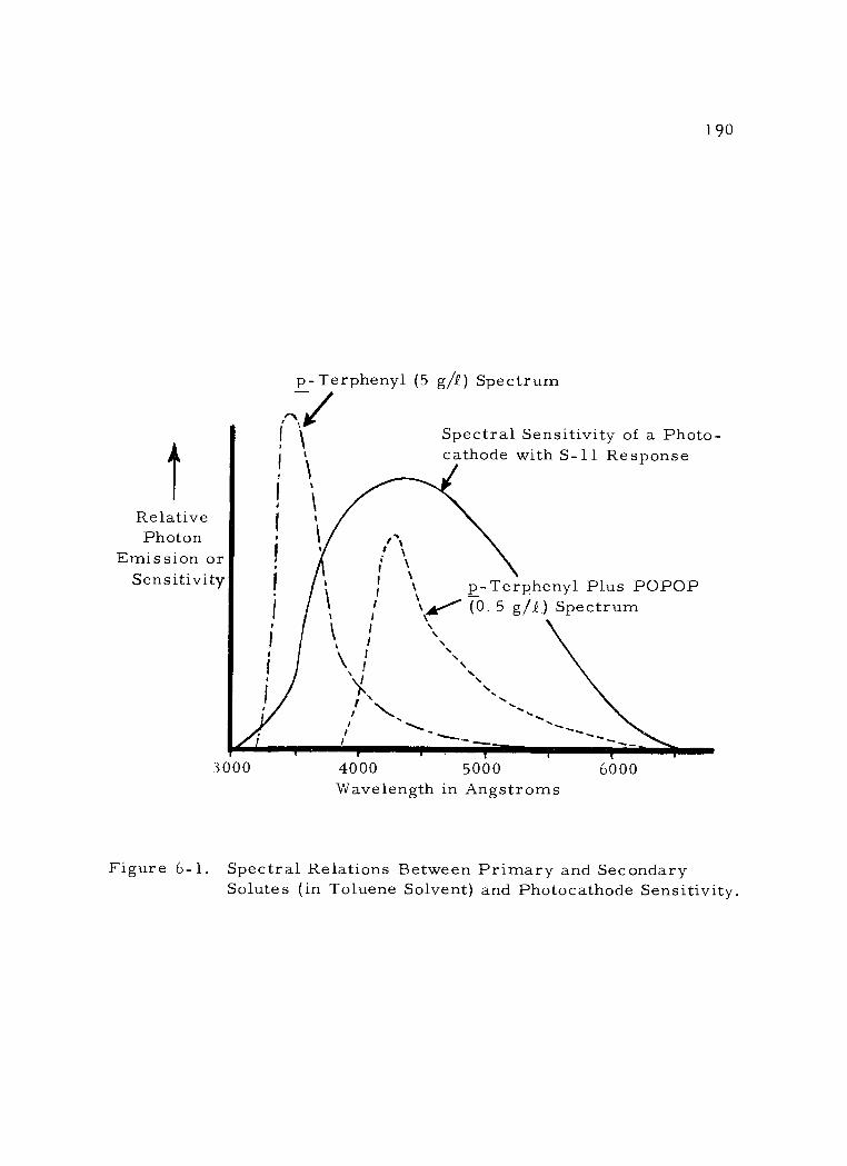
Relative Photon
Emission or Sensitivity
p-Terphenyl (5 g.Q) Spectrum
,i I 1
iA
P- P Y Ter hen l Plus POPOP A/ (0. 5 g /i) Spectrum
190
Spectral Sensitivity of a Photo- cathode with S -11 Response
I . I . \ I . . . .
` N ` \ / . \ `. . i ` .
3000 4000 5000 Wavelength in Angstroms
6000
Figure 6 -1. Spectral Relations Between Primary and Secondary Solutes (in Toluene Solvent) and Photocathode Sensitivity.
` g \
\ ' `
`
I
\ /
I
I
(
191
solution. According to Hayes and Ott (43, p. 9), the fluor
solution specified above will yield about seven photons per
Key of beta particle energy. The 50 Key beta particle un-
der consideration would then yield approximately 350 pho-
tons.
(2) A fraction of these fluorescence photons do not reach the
adjacent photocathode surface. Instead they are lost by
absorption in the solution, the counting bottle, or the re-
flector, or by scattering at the air -glass interfaces. As-
suming that such loss approximates 15 percent, about 297
photons would impinge on the photocathode.
(3) If the conversion efficiency of the photocathode averages
ten percent, then about 29 photoelectrons would be pro-
duced and be subjected to the multiplication mechanism of
the dynode series.
(4) A photomultiplier with an amplification factor of 106 would
then produce 2. 9 x 10⁷ electrons at the output, which is
equivalent to a charge of about 4. 6 x 10 -12 coulombs.
This charge could give rise to a pulse of about 150 milli-
volts. This figure should be contrasted with the value cal-
culated for a 1. 17 Mev gamma ray on page 167.
192
Due to the difficulty of detecting a pulse of this small size, it
is necessary to use an external amplifier of higher gain than required
for gamma detection with crystal fluors. It should also be remember-
ed that the above calculations are for a C14 beta particle having an en-
ergy equivalent to its E n meaHalf of the beta particles from a C14
sample would be emitted with lower energies. By comparison, fol-
lowing the same calculations as above, a beta particle from H3 emitted
at E (5. 5 Key) would yield an output pulse from the photomulti- mean
plier of only about 18 millivolts in size. Lukens (62) presents further
discussion of these quantitative relationships.
Depending on the photocathode sensitivity and the degree of ab-
sorption loss a given minimum number of photons will be required to
result in the ejection of one photoelectron from the photocathode. Beta
particles of such low kinetic energy that they result in the emission of
less than that minimum number of photons from the fluor solution will
not lead to an output pulse. In the circumstances specified in the pre-
vious example this minimum energy level would be over 1, 600 ev.
Thus, a sizeable fraction of the beta particles from a tritium -labelled
sample would have insufficient energy to be detected by the liquid scin-
tillation process. In addition, many of the pulses derived from tri-
tium beta particles would be of the same energy as thermionic noise
pulses of the photomultiplier and indistinguishable from them. This
193
and other factors that limit sensitivity in liquid scintillation counting
are discussed by Swank (11, p. 23 -38).
B. Evaluation of the Internal - Sample Scintillation Method
1. Advantages of liquid scintillation counting
In liquid scintillation detection, as in external -sample scintilla-
tion detection, the size of the photomultiplier output pulse is directly
related to the magnitude of energy associated with the radiation inter-
acting with the scintillation medium. This relationship allows an anal-
ysis of the spectrum of beta emitters. An advantage of this propor-
tionality of pulse size to particle energy is the possibility of differen-
tiating between radiation from two different beta -emitting isotopes in
the same sample (a double - labeled sample). In order for this to be
possible the maximum beta energies of the two nuclides must differ by
a factor of at least four. Samples labeled with both C14 and H3 are
most commonly encountered. A treatment of the methods of counter
operation in such determinations is beyond the scope of this book. For
further information the reader is referred to the excellent discussion
by Okita, et al. (65).
Another advantage of using fluor solutions for detection instead
of inorganic crystalline fluors lies in the very much faster photon de-
cay times of the former (50). Fluorescence in most crystalline fluors
194
decays relatively slowly. Harrison (37) found up to eight percent of
the peak fluorescence in a NaI (T1) crystal persisting at 200 micro-
seconds following the initial gamma interaction. By contrast, only
one percent of the fluorescence in a toluene -p- terphenyl solution re-
mained after O. 3 microseconds! This characteristic of scintillator
solutions allows their use with "fast" amplifiers, avoiding coincidence
loss at even very high counting rates.
The most significant application of liquid scintillation detection
is for the assay of beta - emitting samples, especially those with low
energies. Because of the intimate relation of radioactive sample and
fluor solution, virtually all sample disintegrations are detected. The
complicating factors of self- absorption, window absorption, geometry,
and backscatter that plague traditional G -M assay of weak beta sam-
ples are virtually eliminated (see Chapter 9). For this reason, the
major current application of liquid scintillation detection involves as-
say of H3, C14, S35, or Ca45. Under optimal conditions, C14 detec-
tion efficiency may reach 90 percent. Because of the large proportion
of very low energy beta particles it emits, tritium is seldom detected
with an efficiency exceeding 30 percent. Counting efficiencies are af-
fected markedly by the nature of the sample -fluor solution and the
mode of counter operations as will be described later.
195
While scintillation solutions have been chiefly used for detect-
ing low energy beta particles, they have detection efficiencies ap-
proaching 100 percent for alpha particles. Unfortunately, nearly all
alpha emitters are nuclides of high atomic weight and, as such, are
insoluble in the aromatic hydrocarbon solvents used. Thus, unusual
sample preparation procedures must be employed as will be described
in Chapter 8. By contrast, medium to high energy gamma rays are
poorly detected by small - volume fluor solutions because of the much
lower energy absorbing capabilityof liquids as compared to solids. On
the other hand, an isotope which emits only weak x -rays, such as Fe 55,
would be difficult to assay by any other method than liquid scintillation
detection. High energy gamma radiation may, however, be detected
with reasonable efficiency by large volume ( "giant ") liquid scintillators,
such as the whole body counters designed for clinical use.
2. Problems inherent in liquid scintillation counting
a. Photomultiplier thermal noise: In liquid scintillation detec-
tion the pulse size from low energy beta particles is so small that in-
terference from photomultiplier thermal noise must be minimized. A
photocathode in complete darkness may emit on the order of 5, 000
photoelectrons /cm2 /second at room temperature. It is clearly desir-
able to minimize the resulting photomultiplier "dark current ".
196
Cooling the photomultiplier will reduce this noise level by a factor of
nearly two for every 10° C near room temperature. Thus, it is com-
mon practice to operate the detector in a freezer at temperatures of
0 - 5° C. As a further complication, attention must then be given to
the choice of scintillation solutions that will not freeze at such reduced
temperatures.
Since most "noise" pulses are of very low energy, the simplest
means of preventing a liquid scintillation counter from registering
them is to include a discriminator circuit ( "low gate ") that rejects
pulses below a given minimal energy level. It should be noted that
such a "low gate" does not actually reduce photomultiplier dark cur-
rent, as does cooling, but simply prevents it from being counted.
However, this is not completely effective when a very low energy beta -
emitting isotope, such as tritium, is being assayed. Here, a sizeable
fraction of the pulses resulting from the tritium beta particles are of
the same energy level as the photomultiplier noise pulses. Thus,
other means must be employed to selectively reject noise pulses.
In another method of minimizing thermal noise counts, two
photomultipliers are arranged so that they view the same vial of sam-
ple-fluor solution. This pair of photomultipliers (the "analyzer" and
the "monitor ") is connected through a coincidence circuit which is ar-
ranged to allow a "count" to be registered only when a pulse arrives
197
simultaneously from each photomultiplier. Thus, a noise signal from
only one photomultiplier is not registered, unless by coincidence an-
other noise pulse originates in the other tube within the resolving time
of the circuit. Since thermal noises are random events and the circuit
resolving time is of the order of 10 -7 seconds, the background due to
thermionic emission is reduced from perhaps several hundred thou-
sands counts per minute to only a few counts per minute. A minimal
disadvantage of the coincidence arrangement is that it also reduces
slightly the detection sensitivity, since a minimum of two photons are
now required to yield a detectable signal. This is particularly impor-
tant in the detection of tritium, since a sizeable number of the beta
particles from tritium are too low in energy content to give rise to the
emission of two photons simultaneously.
b. Counting sample preparation: Another complication of li-
quid scintillation counting concerns sample preparation. The most
efficient scintillation solvents are aromatic hydrocarbons which are
not readily miscible with aqueous samples. In addition many of the
common biological compounds are polar in nature and will not dissolve
in such non -polar solvents as toluene. Then a certain amount of vir-
tual "witchcraft" is called for in concocting a suitable scintillation sol-
vent mixture. In general, each new compound to be assayed must be
investigated for its behavior in any given solvent system and the proper
198
solvent mixture must be determined by prior experimentation. Never-
theless, once a proper scintillation solvent is found the preparation of
samples for liquid scintillation counting is a relatively simple proce-
dure. This ease of routine sample preparation is, in fact, one of the
significant advantages of this means of detection.
c. Quenching: A persistent problem in liquid scintillation de-
tection is the effect known as "quenching ". Broadly defined, quench-
ing is any reduction of efficiency in the energy transfer process in the
scintillation solution. Thus, quenching results in a decreased light
output per beta particle and, consequently, the production of a smaller
output pulse in the photomultiplier, or even failure to yield a detec-
table pulse. The net effect of quenching is, therefore, a reduction of
detection efficiency. Furthermore, since the extent of quenching var-
ies considerably with different sample materials, comparison of acti-
vity determinations from varied sample types is rendered unreliable.
Thus, a determination of just how much the counting efficiency of ev-
ery sample has been decreased by quenching must be made (see pages
221 -227).
Quenching may occur by any of several mechanisms. The
counting sample (most commonly), or other components of the scintil-
lation solution, may absorb some of the energy associated with the
beta particle and degrade it to a form not capable of exciting the fluor

199
(chemical quenching). Any nonfluorescent solute molecules, particu-
larly the polar compounds, are potentially quenching agents, since they
may absorb energy from the excited solvent molecules without emitting
photons. On the other hand, quenching may occur simply as a result of
dilution of the fluor solution by the counting sample and, hence, a reduc-
tion of the probability of scintillation events (dilution quenching). Even if
energy transfer from solvent to fluor is not reduced, colored sample ma-
terials will absorb some of the fluorescence photons before they leave the
counting vial (color quenching). Herberg's study of this phenomenon is
particularly valuable (48). Both chemical and color quenching are as so-
ciated with the molecular structure of the sample material, whereas dilu-
tion quenching is related largely to sample concentration. Certain other
effects may also result in photon quenching, such as separation of the
fluor solution into two liquid phases, partial freezing of the solution,
or fogging of the outside of the sample vial (optical quenching).
Certain substances exert a more pronounced quenching action
than others. Oxygen, water, halogenated compounds, and polar com-
pounds in general could be listed as severe quenchers. It is the vari-
able presence of these agents in most biological samples that accounts
for the somewhat empirical selection of proper scintillation solutions.
Kerr, et al. (56), have investigated and tabulated the quenching effects
of a large number of organic compounds. Helmick (47) described the
200
quenching effect of benzoic acid. The latter study is of importance
since labelled benzoic acid is often used as an internal standard in li-
quid scintillation counters to determine counting efficiency (see page
223)
The quenching effect of dissolved oxygen in the scintillation
solution was first pointed out by Pringle, et al. (70). Seliger, et al.
(85), and Berlman (12) subsequently investigated the mechanism of
oxygen quenching and found it to result from collision transfer of en-
ergy from the solvent to oxygen. Since oxygen is an incidental con-
taminant and not a part of the sample, various means have been de-
vised to remove it from the fluor solution (98). These have included
bubbling argon gas (66), carbon dioxide (71), or nitrogen through the
solution, or, in addition, using ultrasonic degassing (22). As a means
of reducing chemical quenching by ethanol, ultraviolet irradiation has
been suggested (61). In general practice the problem of quenching is
solved, not by avoiding or eliminating the quenching agent, but rather
by devising a reliable method to estimate the precise extent of quench-
ing.
Despite the drawbacks mentioned, the liquid scintillation me-
thod of detection is the most generally effective means for assaying
low energy beta -emitting samples, especially H3 and C14 (11, p. 288-
292). In view of the ubiquitous occurrence of the latter two elements
201
in living organisms, this detection method is of paramount importance
to the biologist using radiotracers. The relative ease of sample pre-
paration, the versatility of sample form possible, 47 detection geo-
metry and the commercial availability of reliable counting systems
with high capacity automatic sample changers render this detection
method the most useful where large numbers and types of samples
must be assayed.
C. Components of an Internal- Sample Scintillation Counter
A typical liquid scintillation counting assembly is diagrammed
in Figure IV -1. It will be readily seen that a complete liquid scintilla-
tion counter is far more complex than the other counting assemblies
previously described (Chapters 4 -5). The liquid scintillation counter
is divisible into two major units: the detector assembly and the oper-
ating mechanism. The detector components will be discussed fully in
this chapter, while an extended discussion of the operating mechanism
(1 1 , p. 41-80) will be delayed to Experiment IV.
1. The operating mechanism
In brief it will be noted that in the operating mechanism the
function of the "monitor" photomultiplier and its associated linear
amplifier and discriminator is to actuate the coincidence circuit. The

202
coincidence circuit, in turn, provides momentary signals to the two
analyzers, which then allow passage of coincidental pulses from the
"analyzer" photomultiplier. Pulses from the "analyzer" photo multiplier
are passed through a dual set (channels one and two) of linear ampli-
fiers, discriminators, and analyzers to separate scalers. The dis-
criminator levels in these two channels are independently adjustable,
allowing examination of overlapping, or entirely separate portions of a
beta energy spectrum.
2. The detector assembly
With regard to the liquid scintillation detector assembly alone,
there are certain basic differences between its components and those
of an external - sample scintillation detector as discussed in Chapter 5.
These differences center primarily on the composition of the fluor
(solution vs. crystal). However, different optical relations must also
be considered since the photomultiplier is exposed to a succession of
fluor solutions, rather than remaining optically coupled to an enclosed
crystal fluor.
a. Optical components: The photomultiplier (24, p. 198 -215),
or two with coincidence circuitry, is mounted in a light -tight shield so
that it views the sample vial. An arrangement must be incorporated to
prevent light reaching the photocathode when samples are changed.
203
Optical coupling of the sample vial and the surface of the photomulti-
plier tube is not usually attempted, but the sample chamber is nor-
mally coated with a light- reflecting surface to direct the maximum
light to the photocathode. A variety of substances have been used as
coating materials, of which titanium dioxide appears to be the most
generally effective (7).
The sample holding vial is normally made of glass. However,
ordinary glass contains a considerable quantity of the natural radio-
isotope K40, which thus contributes significantly to the background
count rate. For this reason, it is common practice to employ sample
vials made from special low potassium glass. Quartz glass has also
been used (1), but its cost is prohibitive except where extremely low
backgrounds are essential and few samples are involved. Medium
density polyethylene vials have been suggested (59) as both inexpensive
and not contaminated with K40. Rapkin (73) reports an increase in
H3 detection efficiency with such vials, but also finds them permeable
to toluene (the common fluor solvent) and thus of limited usefulness.
b. Fluor solution components: The actual preparation of
samples will be described in Chapter 8, however, the components of
the scintillation solution, excluding the sample itself, will be discuss-
ed at this point. The bulk of the scintillation solution consists of a
primary solvent, with small quantities of primary solute and
204
secondary solute (the wave- shifter). Both of the solutes are fluors.
Depending on the nature of the sample in question, a secondary sol-
vent may also be employed.
(1). Primary solvents: The role of the primary solvent is to
absorb energy from the beta particles and transfer it to the fluor.
Consequently, an efficient scintillation solvent must have good energy
transfer characteristics, as well as a small absorption coefficient for
the light emitted by the fluor. Another important attribute of the sol-
vent is that it should have a good chemical solvent power for a wide
variety of sample materials. Since the majority of biological samples
are polar compounds and soluble in water, it is highly desirable that
the primary solvent be water miscible. Unfortunately, few solvents
have been found with both these characteristics. A third consideration
is that the solvent should not freeze at counting temperatures. Other-
wise, the operating temperature of the photomultiplier, cooled to re-
duce thermal noise, may be limited by the freezing point of the solvent
in use. The purity of the scintillation solvent used cannot be over-
emphasized. Any degree of quenching from contaminants in this com-
ponent will greatly reduce detection efficiency.
The most efficient compounds investigated as scintillation sol-
vents are aromatic hydrocarbons of alkylbenzene structure (xylene,
toluene, etc. ). Of these, toluene is the most widely used.
205
Unfortunately, if suffers from the twin disadvantages of low flash
point and poor miscibility with water. A variety of substitutes for tol-
uene have been proposed (64), with either lessened fire hazard or bet-
ter solvent powers. For one reason or another none have replaced it
as yet.
A second group of compounds which are generally less effi-
cient, but very useful for certain sample types, is the aromatic ethers.
Anisole and 1, 4- dioxane, with respective efficiencies of 80 percent
and 70 percent relative to toluene, are commonly employed. Dioxane
is especially useful because it is water miscible. A problem of
freezing exists with this solvent, however, as its freezing point is
+12° C.
(2). Secondary solvents: Solvent mixtures may be used to
solubilize radioactive samples which are not soluble in a good primary
solvent, or to increase the energy transfer efficiency of an inferior
primary solvent which has desirable solvating properties. As an ex-
ample, the addition of small amounts of ethanol (or methanol) to a tol-
uene primary solvent improves considerably its ability to incorporate
aqueous samples, without causing excessive loss of scintillation effi-
ciency. By contrast, where dioxane has been used as a primary vol-
vent because of its miscibility with water, its lower energy transfer
efficiency may be improved by the addition of relatively small

206
quantities of naphthalene. Furst and Kallman (30) have evaluated the
factors that affect energy transfer in such scintillation solvent mix-
tures.
Secondary solvents of another important class serve as speci-
fic binding agents for various inorganic substances. These fall into
several categories. Metallic ions, for example, may be incorporated
into metal - organic complexes which are readily soluble in aromatic
hydrocarbons. To date the best organic complexing agents to be used
with liquid scintillator systems are the acidic esters of orthophos-
phoric acid, i. e. , dibutyl phosphate, dioctyl phosphate, etc. Metallic
ions may also be converted to salts of 2- ethylhexanoic acid (octoic
acid), which are reasonably soluble in aromatic hydrocarbons.
Of particular importance to the biologist are the binding agents
for CO2. Several organic compounds have been employed to trap the
gas and convert it to a toluene -soluble carbonate. A methanolic solu-
tion of the hydroxide of "Hyamine 10 -X" [ p- (diisobutylcresoxethoxy -
ethyl)- dimethylbenzyl- ammonium chloride ] (Rohm & Haas, Inc. ) has
been the most widely used for this purpose. More recently "Primene
81 -R" (Rohm & Haas, Inc. ), ethanolamine, and ethylene diamine have
been employed for reasons of economy and reduced quenching. Speci-
fic scintillation solvent formulations involving these substances will
be found in Tables 8 -2, 8 -3 and 8 -4.
207
(3). Primary solutes: This component of the scintillation so-
lution is the fluor which must efficiently convert excitation energy to
light quanta. During recent years a most extensive search has been
conducted, largely by the Biomedical Research Group at the Los
Alamos Scientific Laboratory, for compounds with suitable fluor qual-
ities (4, p. 8 -9, 13 -14, 31 -35, 38 -40, 44, 57 -58, 67 -68, 71, 94 -95).
In 1958, Hayes, et al. , (44) listed 483 different compounds that had
been investigated.
A common characteristic of the most efficient fluors is that
they contain three, and preferably four, aromatic or heterocyclic
rings linked together in a linear manner that allows continuous conju-
gation throughout the molecule (35). In addition to being an efficient
light emitter, the fluor should produce a photon spectrum suited to
the photocathode sensitivity and be soluble over a range of tempera-
tures and with a variety of solutions. It is further desirable that it be
economical in cost. In general, for a given solvent, the counting effi-
ciency increases with increasing fluor concentration. Some fluors,
however show the desirable characteristic of reaching a concentra-
tion giving constant detection efficiency prior to the solubility limit,
where efficiency is independent of concentration.
The most efficient fluors fall into the class of oligophenylenes,
oxazoles, or oxadiazoles (11, p. 101 -107). Because of the complexity

208
of standard chemical nomenclature for these classes of compounds,
an abbreviated system has been devised to describe them. The letter
"P" is used for phenyl, "N" for naphthyl, "B" for biphenyl, "O" for
oxazole, and "D" for the oxadiazole group.
Despite the large number of potential fluors investigatedfonly
three have proven worthy of consideration for practical use. The
first substance so employed, para- terphenyl, is particularly attrac-
tive because of its relatively low cost. However, for many applica-
tions its solubility is too low. This is especially true when water is
loaded into the liquid scintillator or the solution must be cooled to low
temperatures. For these reasons it has been generally replaced by
PPO (2, 5- diphenyloxazole) (38). PPO, because of its good solubility
at low temperatures, has become the most popular primary solute
for counting with cooled coincidence counters, despite its cost. PPO
has a relative pulse height three percent greater than p- terphenyl. A
third compound, PBD (phenylbiphenyloxadiazole), is the most effi-
cient primary solute, with a relative pulse height 24 percent greater
than p- terphenyl. However, it also has the disadvantage of limited
solubility and high cost. In such fluor efficiency comparisons, p-
terphenyl is arbitrarily assigned a relative pulse height value of 1. 0.
These three fluors have photon emission peaks in the neighborhood of
3460 A, 3800 A, and 3700 A, respectively, and should therefore be
209
used with wave shifters.
(4). Secondary solutes: This component acts as a secondary
fluor whose effect is to shift the wave length of the light emitted by
the primary fluor to a region of greater photocathode sensitivity (see
Figure 6 -1). The secondary solutes are usually too insoluble, too
expensive, or have too great a degree of self- quenching to function as
primary solutes. They are useful because addition of only minute
quantities to the scintillation solution may give impressive increases
in counting efficiency. In general, their concentrations in the scintil-
lation solution are only about 1100 those of the primary solutes.
Hayes, et al. (41), have evaluated the merits of a large number of
compounds for use as wave shifters.
Several secondary solutes have found common use. POPOP
[ 1, 4- bis- 2- (5- phenyloxazolyl)- benzene] is by far the most widely
employed at present. Dimethyl -POPOP [1, 4- bis -2(4- methyl -5-
phenyloxazolyl)- benzene has become available more recently and has
the advantages of better solubility and longer wave length of photon
intensity peak compared to POPOP. A third compound, a -NPO [2-
(a- naphthyl)- 5- phenyloxazole) , has found limited popularity, but is
not as desirable as the other two compounds. Relative to PPO, these
secondary solutes have pulse heights of 1.45, 1.45, and 1. 21, respec-
tively.

D. Special Types of Liquid Scintillation Detectors
1. Large volume external- sample detectors.
210
The liquid scintillation detection method is not limited to in-
ternal- samples, although that is the major emphasis of this chapter.
The size restrictions imposed on gas ionization and solid crystal
scintillation detectors do not apply to liquid scintillation detectors.
Very large volumes of scintillation solution may be used with a num-
ber of photomultipliers to produce "giant" detectors (11, p. 246 -257;
36). For a variety of reasons large volume detectors have been con-
structed for use with external sources of radiation. Radiation from
gamma rays, protons, neutrons, and neutrinos has been detected in
this manner.
Of greatest biological interest are the so- called "whole body
counters ", which are used to determine total body radioactivity in
humans or animals. Such measurements give information both on the
natural K40 content of the body (74), and the content of internal radio-
active material accidentally acquired by an individual (92). The Los
Alamos human counter will serve as an example of the immensity of
this detector type. It holds 140 gallons of scintillation solution (tol-
uene- terphenyl -POPOP), uses 108 photomultipliers, and is surrounded
211
by 20 tons of lead shielding (2 -3, 11, p. 211 -219; 24, p. 344 -370).
To increase the efficiency of liquid scintillators for neutron
detection, they have been "loaded" with heavy metals. This has often
required the use of unusual solvents (19). At various times lead, bis-
muth, lithium ( 46 ), uranium, iron, cadmium, and boron have been
employed, but the latter two appear most desirable. In the case of
boron, the reaction B10 (n, a) Li7 occurs, and it is the resultant alpha
particle that is detected by the scintillator (16). It was by means of
such a cadmium loaded scintillator that the neutrino (see Chapter 3)
was first experimentally detected (77). Using paired detectors, only
one of which was sensitive to neutrons, Williams and Hayes (97) devel-
oped a scintillation rate meter for differentiating mixed gamma -neu-
tron radiation from a nuclear reactor.
2. Continuous flow scintillation detectors
An entirely different approach to liquid scintillation type assay
has resulted from the work of Steinberg. In 1958, he introduced an
efficient method for scintillation counting in a two -phase system,
which consisted of a solid, insoluble fluor in intimate contact with an
aqueous solution containing a radioactive sample. At first, he used a
plastic fluor of Pilot Scintillator B (Pilot Chemicals, Inc. ) either in
the form of fine filaments or beads (87) Aqueous sample solutions
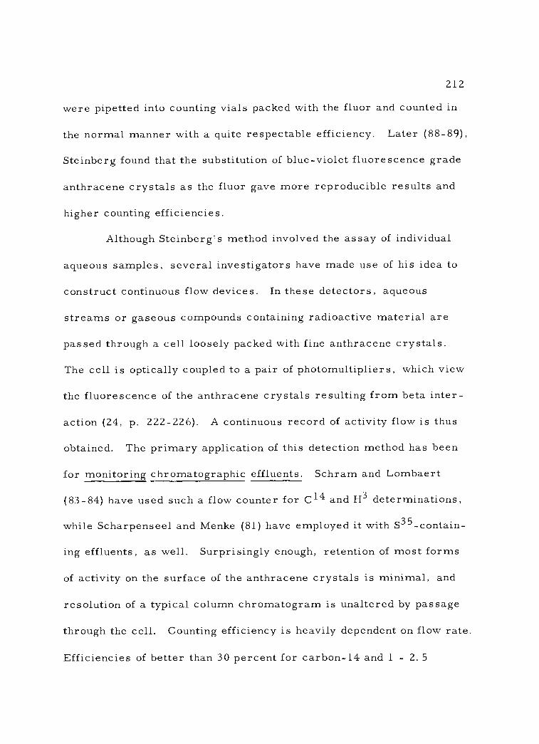
212
were pipetted into counting vials packed with the fluor and counted in
the normal manner with a quite respectable efficiency. Later (88 -89),
Steinberg found that the substitution of blue - violet fluorescence grade
anthracene crystals as the fluor gave more reproducible results and
higher counting efficiencies.
Although Steinberg's method involved the assay of individual
aqueous samples, several investigators have made use of his idea to
construct continuous flow devices. In these detectors, aqueous
streams or gaseous compounds containing radioactive material are
passed through a cell loosely packed with fine anthracene crystals.
The cell is optically coupled to a pair of photomultipliers, which view
the fluorescence of the anthracene crystals resulting from beta inter-
action (24, p. 222 -226). A continuous record of activity flow is thus
obtained. The primary application of this detection method has been
for monitoring chromatographic effluents. Schram and Lombaert
(83 -84) have used such a flow counter for C14 and H3 determinations,
while Scharpenseel and Menke (81) have employed it with S35- contain-
ing effluents, as well. Surprisingly enough, retention of most forms
of activity on the surface of the anthracene crystals is minimal, and
resolution of a typical column chromatogram is unaltered by passage
through the cell. Counting efficiency is heavily dependent on flow rate.
Efficiencies of better than 30 percent for carbon -14 and 1 - 2. 5
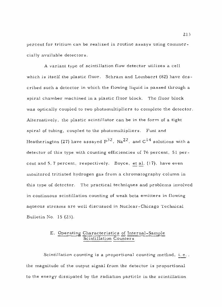
213
percent for tritium can be realized in routine assays using commer-
cially available detectors.
A variant type of scintillation flow detector utilizes a cell
which is itself the plastic fluor. Schram and Lombaert (82) have des-
cribed such a detector in which the flowing liquid is passed through a
spiral chamber machined in a plastic fluor block. The fluor block
was optically coupled to two photomultipliers to complete the detector.
Alternatively, the plastic scintillator can be in the form of a tight
spiral of tubing, coupled to the photomultipliers. Funt and
Heatherington (27) have assayed P32, Na22, and C14 solutions with a
detector of this type with counting efficiencies of 76 percent, 51 per-
cent and 5. 7 percent, respectively. Boyce, et al. (17), have even
monitored tritiated hydrogen gas from a chromatography column in
this type of detector. The practical techniques and problems involved
in continuous scintillation counting of weak beta emitters in flowing
aqueous streams are well discussed in Nuclear- Chicago Technical
Bulletin No. 15 (23).
E. Operating Characteristics of Internal - Sample Scintillation Counters
Scintillation counting is a proportional counting method, i. e. ,
the magnitude of the output signal from the detector is proportional
to the energy dissipated by the radiation particle in the scintillation

214
solution. Since beta particles are emitted over a continuous energy
spectrum, and in the case of weak betas, vitually all of the particle
energy is given up to the scintillation solution, a pulse height analyzer
is almost universally used with a liquid scintillation detector. This is
an electronic component which accepts and passes on for counting only
pulses of heights falling between two predetermined discriminator lim-
its (the "window" or "channel ")which can be varied by the operator
over an arbitrary voltage scale. Pulse height analysis makes it pos-
sible to select the optimal counter settings under different detection
circumstances, to determine the extent of quenching in a sample and
to simultaneously count the activity in a sample labeled with two dif-
ferent isotopes. Most commercially available counting assemblies
have three or four adjustable discriminators allowing two channel
operation (15). A few counters have three channels.
1. Selection of optimal counter settings
a. Effect of photomultiplier gain and "window" settings: The
size of a detector pulse resulting from a given beta interaction in a
scintillation solution is governed by both the energy of the beta particle
and the gain of the photomultiplier. This gain is directly related to
the potential gradient applied across the dynode chain of the photomul-
tiplier. By increasing this potential, larger pulse sizes will pass
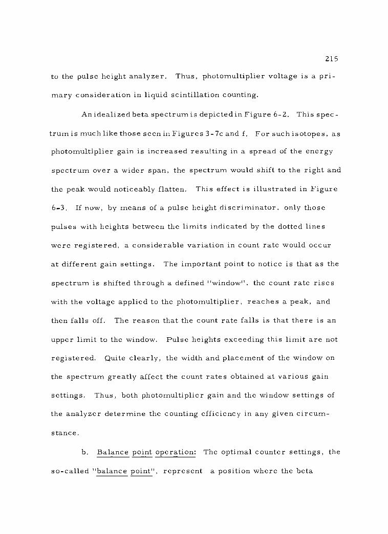
215
to the pulse height analyzer. Thus, photomultiplier voltage is a pri-
mary consideration in liquid scintillation counting.
An idealized beta spectrum is depicted in Figure 6 -2. This spec-
trum is much like those seen in Figures 3 -7c and f. For such isotopes, as
photomultiplier gain is increased resulting in a spread of the energy
spectrum over a wider span, the spectrum would shift to the right and
the peak would noticeably flatten. This effect is illustrated in Figure
6 -3. If now, by means of a pulse height discriminator, only those
pulses with heights between the limits indicated by the dotted lines
were registered, a considerable variation in count rate would occur
at different gain settings. The important point to notice is that as the
spectrum is shifted through a defined "window ", the count rate rises
with the voltage applied to the photomultiplier, reaches a peak, and
then falls off. The reason that the count rate falls is that there is an
upper limit to the window. Pulse heights exceeding this limit are not
registered. Quite clearly, the width and placement of the window on
the spectrum greatly affect the count rates obtained at various gain
settings. Thus, both photomultiplier gain and the window settings of
the analyzer determine the counting efficiency in any given circum-
stance.
b. Balance point operation: The optimal counter settings, the
so- called "balance point ", represent a position where the beta
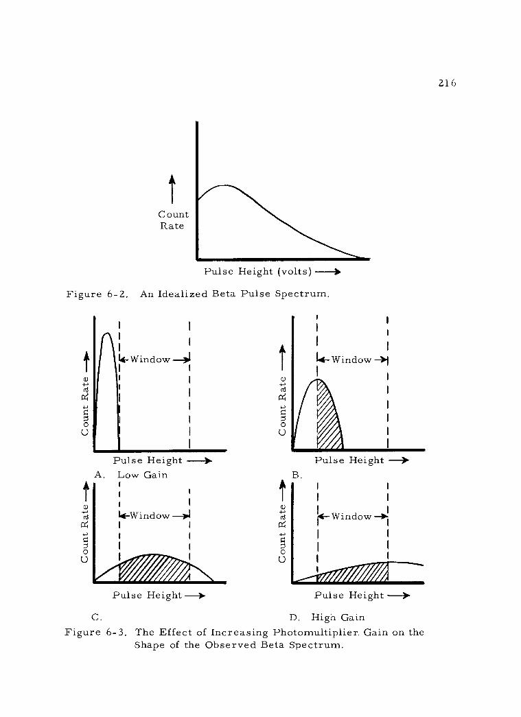
Count Rate
Count Rate
216
Count Rate
Pulse Height (volts) --) Figure 6 -2. An Idealized Beta Pulse Spectrum.
t
I
I4-Window -
Pulse Height -) A. Low Gain
0 1
I - Window --J
ffìJr/I Pulse Height
r
B.
Pulse Height - 4- Window -
Pulse Height -) C. D. High Gain
Figure 6 -3. The Effect of Increasing Photomultiplier. Gain on the Shape of the Observed Beta Spectrum.
Ì
I I
I
T
a I
G
I
i
I
(
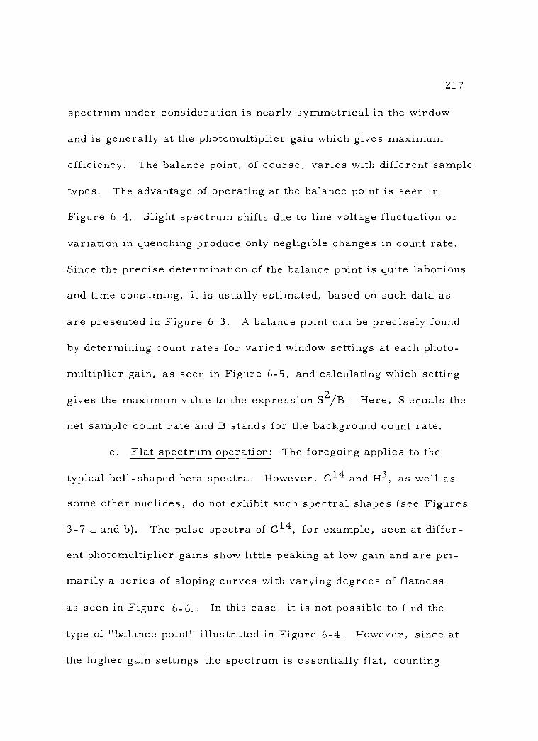
217
spectrum under consideration is nearly symmetrical in the window
and is generally at the photomultiplier gain which gives maximum
efficiency. The balance point, of course, varies with different sample
types. The advantage of operating at the balance point is seen in
Figure 6 -4. Slight spectrum shifts due to line voltage fluctuation or
variation in quenching produce only negligible changes in count rate.
Since the precise determination of the balance point is quite laborious
and time consuming, it is usually estimated, based on such data as
are presented in Figure 6 -3. A balance point can be precisely found
by determining count rates for varied window settings at each photo-
multiplier gain, as seen in Figure 6 -5, and calculating which setting
gives the maximum value to the expression S2 /B Here, S equals the
net sample count rate and B stands for the background count rate.
c. Flat spectrum operation: The foregoing applies to the
typical bell- shaped beta spectra. However, C14 and H3, as well as
some other nuclides, do not exhibit such spectral shapes (see Figures
3 -7 a and b). The pulse spectra of C14, for example, seen at differ-
ent photomultiplier gains show little peaking at low gain and are pri-
marily a series of sloping curves with varying degrees of flatness,
as seen in Figure 6 -6.. In this case, it is not possible to find the
type of "balance point" illustrated in Figure 6 -4. However, since at
the higher gain settings the spectrum is essentially flat, counting

Count Rate
A B
A These pulse heights shifted into window
218
Pulse Heights (Volts
Figure 6 -4. Balance Point Operation -- Effect of Spectrum Shift.
Count Rate
10- co v. window
10-100 v. window 10-70 v. window
10 -50 v. window
10 -30 v. window
Photomultiplier Potential (Volts)--).
Figure 6 -5. Balance Point Determination -- Effect of Window Width on Count Rate.
4-- Window -OBI i
--'
These pulse heights I
shifted o of window
/ /
1
I
i
B.
/ y
->

Lowest Gain
Count Rate
Highest Gain
- -_
Pulse Height (Volts) -v.
219
Figure 6 -6. Pulse Spectra of C14 at Different Photomultiplier Gain Settings.
J
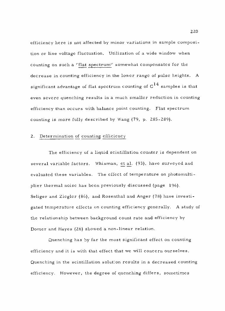
220
efficiency here is not affected by minor variations in sample composi-
tion or line voltage fluctuation. Utilization of a wide window when
counting on such a "flat spectrum" somewhat compensates for the
decrease in counting efficiency in the lower range of pulse heights. A
significant advantage of flat spectrum counting of C14 samples is that
even severe quenching results in a much smaller reduction in counting
efficiency than occurs with balance point counting. Flat spectrum
counting is more fully described by Wang (79, p. 285 -289).
2. Determination of counting efficiency
The efficiency of a liquid scintillation counter is dependent on
several variable factors. Whisman, et al. (93), have surveyed and
evaluated these variables. The effect of temperature on photomulti-
plier thermal noise has been previously discussed (page 196).
Seliger and Ziegler (86), and Rosenthal and Anger (78) have investi-
gated temperature effects on counting efficiency generally. A study of
the relationship between background count rate and efficiency by
Domer and Hayes (26) showed a non - linear relation.
Quenching has by far the most significant effect on counting
efficiency and it is with that effect that we will concern ourselves.
Quenching in the scintillation solution results in a decreased counting
efficiency. However, the degree of quenching differs, sometimes

221
greatly, from one type of sample to another. Although it is some-
times possible to greatly reduce quenching by proper selection of
scintillation solutions, it is always necessary to determine the extent
of quenching, if counting results from one sample type are to be com-
pared with those from others. Several methods for such determina-
tions have been developed (91).
a. Internal standardization method: The oldest method of ef-
ficiency determination is known as internal standardization, or "spiking ".
It consists of adding a precisely known amount of the same isotope (an "in-
ternal standard ") in a non - quenching form to a previously counted sample.
The resulting mixture is then recounted. The counting efficiency of
the quenched sample can then be determined as follows:
(Equation 6 -1) Efficiency =
Net count rate -Net count rate (int. std. + sample) (sample)
Disintegration rate (int. std. )
A variety of compounds have been employed as internal stand-
ards. Toluene -C14, n- hexadecane -C14, benzoic acid -C14, tritiated
toluene, tritiated water, and tritiated n- hexadecane are all commer-
cially available for this purpose. Williams, et al. (96), and Marlow
and Medlock (63) have described techniques for preparing the benzoic
acid -C14 standard. Unfortunately, each standard has its drawback.
Accurate pipetting of toluene is difficult, while benzoic acid and water

222
are themselves quenching agents.
The internal standardization method suffers from several dis-
advantages. It is time consuming in that two counts are required per
sample, and the sample vial must be opened between the counts.
Furthermore, the accuracy of the determination is often dependent on
the accurate measurement of small volumes of liquid. Additional sta-
tistical complications occur if the activity of the sample and standard
differ greatly.
b. Dilution method: Another means of determing efficiency
involves counting several different dilutions of the radioactive sample
in the fluor solution. A plot of cpm /ml against sample concentration
is then prepared and extrapolated to infinite dilution, where no sample
quenching would exist. This method is likewise time consuming and
subject to considerable manipulative error. Peng (24, p. 260 -275)
has presented an excellent evaluation and comparison of the internal
standard and dilution methods of determining counting efficiency.
c. Pulse height shift method: When quenching occurs the
average energy of the beta pulse spectrum decreases and, conse-
quently, the entire beta spectrum shifts toward a lower energy level
(see Figure 6 -7 c). Baillie (6), in 1960, first suggested a practical
means for relating the degree of this pulse height shift to the extent of
quenching. Bruno and Christian (18) subsequently refined the
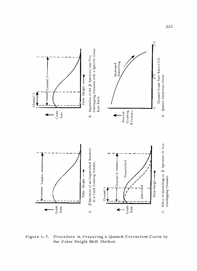
aQ
iE --
---
1
Win
dow
---r
co
Puls
e H
eigh
t ->
A
. 13
Sp
ectr
um o
f an
Unq
uenc
hed
Stan
dard
in
a T
otal
Cou
ntin
g W
indo
w.
Cou
nt
Rat
e
Cha
nnel
1
-- Channel
2 --
-1
I
I
Unq
uenc
hed
Puls
e H
eigh
t --I
I.
C.
Eff
ect
of Q
uenc
hing
on
13
Spec
trum
in
Tw
o
Ove
rlap
ping
Cha
nnel
s.
Cou
nt
R a
te
Cha
nnel
1
i_
'I
I
I ' C
hann
el 2
----
Puls
e H
eigh
t -
B.
Sepa
ratio
n of
the
(3
Spec
trum
int
o T
wo
Ove
rlap
ping
Cha
nnel
s w
ith a
Spe
cifi
c C
ount
R
ate
Rat
io.
Perc
ent
Cou
ntin
g E
ffic
ienc
y
Incr
ease
d Q
uenc
hing
0 0.
5 C
hann
el C
ount
Rat
e R
atio
(1/
2)
D.
Que
nch
Cor
rect
ion
Cur
ve.
r4'
Cou
nt
o t n
Rat
e
sz
m
r!
CD
11
(D
K
(D
n r ó n >
I
I
I
1.0
224
technique. Currently the terms "pulse height shift" and "channels
ratio" method are interchangeably used in respect to the procedure.
Briefly, the method may be outlined as follows: (1) On a dual
channel liquid scintillation spectrometer a counting window is set up
to cover virtually all the beta spectrum of an unquenched standard
sample above the noise level (Figure 6-7a). (2) The discriminators
are now reset to give two counting windows. Channel 1 covers only
the lower half of the energy spectrum, while channel 2 encompasses
nearly the whole spectrum as above (Figure 6 -7 b). Under these con-
ditions a fixed ratio will be obtained between the count rates from the
two channels. (3) Now, standards of known activity in addition to
varying amounts of quenching agent are counted. Because of quench-
ing, the count rate ratio between the two channels will change relative
to the amount of quenching in the samples (Figure 6 -7 c). (4) The
counting efficiency of each sample (net cpm /dpm) is then calculated
and plotted against the respective channel count ratio to produce a
standard quench correction curve (Figure 6-7d). From this curve it
is possible to read directly the counting efficiency for unknown sam-
ples of the same isotope, when their channel counting ratio is known.
The advantages of this method are evident (20). A single
quench correction curve for either C14 or H3 has been found sufficient
to cover many of the common chemical quenching agents, although it

225
will not account for color quenching. However, such a curve is strict-
ly valid only for the particular counter conditions (photomultiplier
potential, discriminator settings, temperature) and the defined
quenching agent for which it is prepared. A correction curve can be
prepared using a single channel counter, but this is obviously more
time consuming. The pulse height shift method is generally less re-
liable when working with samples whose counting rates are close to
background levels. Practical suggestions concerning the channels
ratio method will be found in Nuclear -Chicago Technical Bulletin No.
13 (21).
F. Summary
Internal - sample scintillation counting has the inherent advan-
tages of high counting efficiency (particularly for low energy beta emit-
ters), energy discrimination, relative ease of sample preparation, and
accommodating relatively large amounts of sample material. Because
of its widespread use for assaying samples containing carbon -14 and
tritium, it is of special importance to the biologist.
Table 6 -1 summarizes pertinent information concerning the
characteristics of the detectors discussed thus far: the ion chamber
with a vibrating -reed electrometer, the proportional detector, the
Geiger -Mueller detector, and both external - sample and
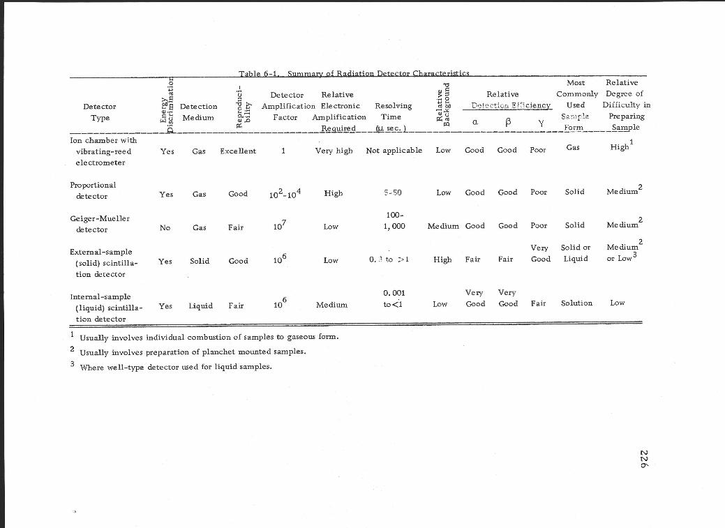
226
Eho3o.s6g.EgH6;;!-i
(, (,)
ddG(dX
troxdE
ooe'dH
9'Bql.li,E
;;=:*BE
;;rlO
PT
H
6
:i E.H
i [EooAool
.d;
==
91986dd€D
D;
HN
CO
tr trm
.1 .rx'd
'oJ6.)
O
aao
'c, o!
'"! rd i
a 15./th
hEX
6Jod
>o
^tpro(,z.ooar)hoop""doo()Eooo
boF
r.dordooo.doo(,= oJo-ordoAGdozb0
ho ooP{
.9E1
"El
s Eg?s
3 *'-bop o b.5P
.rHh
! S;
$,ooq:{do6*
3soov)(!t&
id {1,
.9 E
TT
E
\iOo
.B
E-o
8 f,
#8H€.$?E
E:
z,
3o".]
dtLidC,
F-l(,
.H8
do,oP6io3
(n
o0)
Id
3E *
L\H
O
H9:.1
".,^P-83d'i
eE
6Ee5.gE
-P
Ev
dgq dg-iiUJi
"o0)
E
.90 3
;o'r{ "..1
o\oo
$oI
nto
oalo3oJ
puno,rS4ceg
a^Il"Iall
drurq-lcnpoedag
>l
0l'61
s :il;i
p-rl @-
uil d
boH^
igs;;14
aorF
r
&g<.r Q
.X6E
qH
Iii'3Jv.40
& # E
ee{o
E9
od-3.9
0eI6A
ETE
i.old,
lI
r,rcsr6l)ug
iIIIIIII
No
1,ooo
co0)oxT$doo
troPo0,!0)oh8orooo>6Fa
2#
t g=
u
: e i;$8$ * eE
fo!ore-ord)kk9or0).i-o b0c
x -
fiEH
seS
EU
K
6v-ooX
P
-6'st E
8
227
internal - sample scintillation detectors. While the data listed is of
necessity general, it is based on the forms of these detectors most
commonly used in radiotracer assays.
BIBLIOGRAPHY
1. Agranoff, Bernard W. Silica vials improve low -level counting. Nucleonics 15(10) :106. 1957.
2. Anderson, Ernest C. , et al. A whole body gamma counter for human subjects. 19757 43 p. (U. S. Atomic Energy Commis- sion. LA- 1717).
3. . The Los Alamos human counter. Nucleonics 14(1):26 -29. 1956.
4. Arnold, James R. New liquid scintillation phosphors. Science 122:1139-1140. 1955.
5. Audric, B. N. and J. V. P. Long. Measurement of low energy p- emitters by liquid scintillation counting. Research 5:46 -47. 1952.
6. Baillie, L. A. Determination of liquid scintillation counting effi- ciency by pulse height shift. International Journal of Applied Radiation and Isotopes 8:1 -7. 1960.
7. Bannerman, D. E. and R. J. Lanter. Durable white coating im- proves liquid scintillation counters. Nucleonics 14(2):60 -61. 1956.
8. Barnett, Martin D. , et al. Liquid scintillators. VI. 2 -aryl- and 2, 7- diarylfluorenes. Journal of the American Chemical Society 81:4583 -4586. 1959.
9. . Liquid scintillators. XI. 2-(2-fluorenyl)- 5 -aryl- substituted oxazoles and 2- (2- fluorenyl) -5- phenyl -1, 3, 4- oxadiazole. Journal of the American Chemical Scoeity 82: 2282 -2285. 1960.

228
10. Belcher, E. H. Scintillation counters using liquid luminescent media for absolute standardization and radioactive assay. Journal of Scientific Instruments 30:286 -289. 1953.
11. Bell, Carlos G. , Jr. and F. Newton Hayes (eds. ). Liquid scin- tillation counting. Proceedings of a Conference held at North- western University, Evanston, 1957. New York, Pergamon, 1958. 292 p.
12. Berlman, Isadore B. Luminescence in a scintillation solution excited by a and p particles and related studies in quenching. The Journal of Chemical Physics 34:598 -603. 1961.
13. Birkeland, Stephen P. , et al. Liquid scintillators. X. Some aryl substituted phenanthrenes and dihydrophenanthrenes, and related p- terphenyls and p- quaterphenyls. Determination of Kallman parameters. Zeitschrift für Physik 159:516 -523. 1960.
14. . Liquid scintillators. IX. Synthesis of some aryl substituted phenanthrenes and dihydrophenanthrenes, and related p- terphenyls and p- quaterphenyls. The Journal of Organic Chemistry 26:2662 -2667. 1961.
15. Blau, Monte. Separated channels improve liquid scintillation counting. Nucleonics 15(4):90 -91. 1957.
16. Bollinger, Lowell M. and George E. Thomas. Boron -loaded liquid scintillation neutron detectors. The Review of Scientific Instruments 28:489 -496. 1957.
17. Boyce, I. S. , J. F. Cameron, and K. J. Taylor. A simple plas- tic scintillation counter for tritiated hydrogen. The Interna- tional Journal of Applied Radiation and Isotopes 9:122 -123. 1960.
18. Bruno, Gerald A. and John E. Christian. Corrections for quenching associated with liquid scintillation counting. Analyti- cal Chemistry 33:650. 1961.
19. Buck, Warren L. and Robert K. Swank. Use of isopropylbiphenyl as solvent in liquid scintillators. The Review of Scientific Instruments 29:252. 1958.
229
20. Bush, Elizabeth. General applicability of the channels ratio method of measuring liquid scintillation counting efficiency. American Chemical Society Abstracts 141:27B -28B. Mar. 1962.
21. Bush, Elizabeth T. How to determine efficiency automatically in liquid scintillation counting. Des Plaines, Ill. , 1962. 4 p. (Nuclear- Chicago Technical Bulletin No. 13)
22. Chleck, D. J. and C. A. Ziegler. Ultrasonic degassing of liquid scintillators. The Review of Scientific Instruments 28:466- 467. 1957.
23. Continuous scintillation counting of weak beta emitters in flowing aqueous streams. Des Plaines, Ill. , 1963. , 1963. 4 p. (Nuclear- Chicago Technical Bulletin No. 15)
24. Daub, Guido H. , F. Newton Hayes and Elizabeth Sullivan. (eds. )
Proceedings of the University of New Mexico Conference on Organic Scintillation Detectors, Albuquerque, 1960. Washing- ton, U. S. Government Printing Office, 1961. 417 p. (TID- 7612)
25. Davidson, Jack D. and Philip Feigelson. Practical aspects of internal - sample liquid - scintillation counting. The International Journal of Applied Radiation and Isotopes 2:1 -18. 1957.
26. Domer, Floyd R. and F. Newton Hayes. Background vs. effi- ciency in liquid scintillators. Nucleonics 18(1):100. 1960.
27. Funt, B. L. and A. Hetherington. Spiral capillary plastic scin- tillation flow counter for beta assay. Science 129:1429 -1430. 1959.
28. Furst, Milton and Hartmut Kallman. High energy induced fluo- rescence in organic liquid solutions (Energy transport in li- quids). III. The Physical Review 85:816 -825. 1952.
29. . Energy transfer by means of collision in liquid organic solutions under high energy and ultraviolet exci- tations. The Physical Review 94:503 -507. 1954.
30. . Fluorescent behavior of solutions containing more than one solvent. The Journal of Chemical Physics 23: 607 -612. 1955.
230
31. Gilman, Henry, et al. Some derivatives of aza- aromatic hetero- cycles as liquid scintillator solutes. The Journal of Organic Chemistry 22:1169 -1171. 1957.
32. . Some oxygen- containing heterocycles as liquid scintillation solutes. The Journal of Organic Chemistry 23 :361 -362. 1958.
33. . Some N- arylated heterocycles as liquid scintillation solutes. The Journal of Organic Chemistry. 23: 628 -629. 1958.
34. Gilman, Henry, Eugene A. Weipert and F. Newton Hayes. Some polyaryl derivatives of metals and metalloids as liquid scintillator solutes. The Journal of Organic Chemistry 23: 760 -762. 1958.
35. . Some derivatives of biphenyl as liquid scintillator solutes. The Journal of Organic Chemistry 23:
910 -911. 1958.
36. Harrison, F. B. Large -area liquid scintillation counters. Nucleonics 10(6) :40 -45. 1952.
37. . Slow component in decay of fluors. Nucleonics 12(3) :24 -25. 1954.
38. Hayes, F. N. , R. D. Hiebert, and R. L. Schuch. Low energy counting with a new liquid scintillation solute. Science 116: 140. 1952.
39. Hayes, F. Newton. Liquid solution scintillators. 1953. 75 p. (U. S. Atomic Energy Commission. LA -1639)
40. Hayes, F. Newton, et al. Liquid scintillators. I. Pulse height comparison of primary solutes. Nucleonics 13(12):38 -41. 1955.
41. Hayes, F. Newton, Donald G. Ott, and Vernon N. Kerr. Liquid scintillators. II. Relative pulse height comparisons of sec- ondary solutes. Nucleonics 14(1) :42 -45. 1956.
42. Hayes, F. Newton. Liquid scintillators: attributes and applica- tions. International Journal of Applied Radiation and Isotopes 1:46 -56. 1956.
231
43. Hayes, F. Newton and Donald G. Ott. The small -volume inter- nal- sample liquid scintillation counter. 1957. 37 p. (U. S. Atomic Energy Commission. LA -2095)
44. Hayes, F. N. , et al. Survey of organic compounds as primary scintillation solutes. 1958. 24 p. (U. S. Atomic Energy Commission. LA -2176)
45. Hayes, F. Newton. Solutes and solvents for liquid scintillation counting. Rev. ed. La Grange, Ill. , 1962. 8 p. (Packard Instrument Co. Technical Bulletin No. 1)
46. Hejwowski, J. and A. Szymanski. Lithium loaded liquid scintil- lator. The Review of Scientific Instruments 32:1057 -1058. 1961.
47. Helmick, Marie. The quenching effect of benzoic acid in a li- quid scintillation system. Atomlight (issued by New England Nuclear Corp. ), Feb. 1960, p. 6 -7.
48. Herberg, R. J. Backgrounds for liquid scintillation counting of colored solutions. Analytical Chemistry 32:1468 -1471. 1960.
49. Hodgson, T. S. , B. E. Gordon and M. E. Ackerman. Single -
channel counter for carbon -14 and tritium. Nucleonics 16(7): 89 -94. 1958.
50. Jackson, Jasper A. and F. B. Harrison. A slow component in the decay of the scintillation phosphors. The Physical Review 89:322. 1953.
51. Kallman, Hartmut. Scintillation counting with solutions. The Physical Review 78:621 -622. 1950.
52. Kallman, Hartmut and Milton Furst. Fluorescence of liquids under gamma bombardment. Nucleonics 7(1):69 -71. 1950.
53. . Fluorescence of solutions bombarded with high energy radiation (Energy transport in liquids). The Physical Review 79:857 -870. 1950.
232
54. . Fluorescence of solutions bombarded with high energy radiation (Energy transport in liquids) Part H. The Physical Review 81:853 -864. 1951,
55, Karman, A. and H. R. Tri.tch. Radioas say by gas chromato- graphy of compounds labelled with carbon -14. Nature 186:150- 151. 1960.
56. Kerr, Vernon N. , F. Newton Hayes and Donald G. Ott. Liquid scintillators. III. The quenching of liquid scintillator solu- tions by organic compounds. International Journal of Applied Radiation and Isotopes 1:284 -288. 1957,
57. Kerr, V. N. , et al. Liquid scintillators, VII. 2, 5- diaryl sub- stituted thiazoles as liquid scintillator solutes, The Journal of Organic Chemistry 24:1861 -1864. 1959.
58. . Liquid scintillators, VIII. The effect of the dialkylamino group, The Journal of Organic Chemistry 24:1864 -1866, 1959.
59. Kimbel, K. H, and J. Willenbrink. An inexpensive disposable sample container for single phototube liquid scintillation counting. The International Journal of Applied Radiation and Isotopes 11:157. 1961,
60. Kobayashi, Yutaka. Liquid scintillation counting and some prac- tical considerations. Waltham, Mass. , Tracerlab, 1961. 20 p.
61. Lohmann, W. and W. H. Perkins. Stabilization of the counting rate by irradiation of the liquid scintillation counting solutions with UV- light. Nuclear Instruments and Methods 12:329 -334. 1961.
62. Lukens, H. R. , Jr. The relationship between fluorescence in- tensity and counting efficiency with liquid scintillators. The International Journal of Applied Radiation and Isotopes 12:134- 140. 1961.
63. Marlow, W. F. and R. W. Medlock. A carbon-14 beta -ray stand- ard, benzoic acid -7 -C14 in toluene, for liquid scintillation counters, Journal of Research of the National Bureau of Standards 64A:143-146. 1960.

233
64. Miranda, H. A. , Jr. , and H. Schimmel. New liquid scintillant. The Review of Scientific Instruments 30:1128 -1129. 1959.
65. Okita, George T. , et al. Assaying compounds containing H3 and C14. Nucleonics 15(6):111 -114. 1957.
66. Ott, Donald G. , et al. Argon treatment of liquid scintillators to eliminate oxygen quenching. Nucleonics 13(5):62. 1955.
67. . Liquid scintillators. V. Absorption and fluorescence spectra of 2, 5- diaryloxazoles and related com- pounds. Journal of the American Chemical Society 79:5448- 5454. 1957.
68. . Liquid scintillators. XII. Absorption and fluorescence spectra of 2, 5- diaryl -1, 3, 4- oxadiazoles. The Journal of Organic Chemistry 25:872 -873. 1960.
69. Popják, G. et al. Scintillation counter for the measurement of radioactivity of vapors in conjunction with gas - liquid chromato- graphy. Journal of Lipid Research 1:29 -39. 1959.
70. Pringle, R. W. , et al. A new quenching effect in liquid scintil- lators. The Physical Review 92:1582 -1583. 1953.
71. Protopopov, Kh. V. , et al. New liquid scintillators. Instru- ments and Experimental Techniques 2:200 -204. 1958. (Trans- lated from Pribory i Tekhnika Eksperimenta)
72. Raben, M. S. and N. Bloembergen. Determination of radioacti- vity by solution in a liquid scintillator. Science 114:363 -364. 1951.
73. Rapkin, Edward. Polyethylene containers for liquid scintillation spectrometry. La Grange, Ill. , Packard Instrument Company, n. d. 8 p.
74. Reines, R. , et al. Determination of total body radioactivity using scintillation detectors. Nature 172:521 -523. 1953.
75. Reynolds, George T. , F. B. Harrison and G. Salvini. Liquid scintillation counters. The Physical Review 78:488. 1950.
234
76. Reynolds, George T. Solid and liquid scintillation counters. Nucleonics 10(7):46 -53. 1952.
77. Ronzio, A. R. , C. L. Cowan, Jr. and F. Reines. Liquid scin- tillators for free neutrino detection. The Review of Scientific Instruments 29:146 -147. 1958.
78. Rosenthal, Donald J. and Hal O. Anger. Liquid scintillation counting of tritium and C14 labeled compounds. The Review of Scientific Instruments 25:670 -674. 1954.
79. Rothchild, Seymour (ed. ). Advances in tracer methodology, vol. 1. New York, Plenum Press, 1963. 332 p.
80. Roucayral, Jean C. and Erich Oberhausen. Eine Anordnung zum quantitativen Nachweis von energiearmen p -Strahlern mit fluorezierenden Losungen. Die Naturwissenschaften 42:411- 412. 1955.
81. Scharpenseel, H. W. and K. H. Menke. Radiochromatographie mit schwachen ß- Strahlern (355 14C, 3H). II. Radiosäulen - chromatographie mit Hilfe des Flllssigkeits- Scintillations- Spektrometers. Zeitschrift für Analytische Chemie 182:1 -10. 1961.
82. Schram, E. and R. Lombaert. Determination continue du car - bone-14 et du soufre -35 en milieu aqueux par un dispositif a scintillation. Application aux effluents chromatographiques. Analytica Chimica Acta 17:417 -422. 1957.
83. . Dosage continu du carbone -14 dans les effluents chromatographiques au moyen de poudres d'anthra- cene. Archives Internationales de Physiologie et de Biochimie. 68:845 -846. 1960.
84. Schram, Eric and Robert Lombaert. Determination of tritium and carbon -14 in aqueous solution with anthracene powder. Analytical Biochemistry 3:68 -74. 1962.
85. Seliger, H. H. , C. A. Ziegler, and I. Jaffe. Role of oxygen in the quenching of liquid scintillators. The Physical Review 101:998 -999. 1956.
.

235
86. Seliger, H. H. and C. A. Ziegler. Liquid - scintillator tempera- ture effects. Nucleonics 14(4):49. 1956.
87. Steinberg, Daniel. Radioassay of carbon -14 in aqueous solu- tions using a liquid scintillation spectrometer. Nature 182: 740 -741. 1958.
88. . Radioassay of aqueous solutions mixed with solid crystalline fluors. Nature 183:1253 -1254. 1959.
89. . A new approach to radioassay of aqueous solutions in the liquid scintillation spectrometer. Analytical Biochemistry 1:23 -39. 1960.
90. Swank, Robert K. and Warren L. Buck. Spectral effects in the comparison of scintillators and photomultipliers. The Review of Scientific Instruments 29:279 -284. 1958.
91. Tracerlab, Inc. Quenching in liquid scintillation counting. Waltham, Mass. , 1961. 7 p.
92. Van Dilla, M. A. , R. L. Schuch and E. C. Anderson. K -9: A large 4 n gamma -ray detector. Nucleonics 12(9):22 -27. 1954.
93. Whisman, Marvin L. , Barton H. Eccleston and F. E. Arm- strong. Liquid scintillation counting of tritiated organic com- pounds. Analytical Chemistry 32:484 -486. 1960.
94. Wiley, Richard H. , C. Harry Jarboe, Jr. and F. N. Hayes. Substituted 4, 7- phenanthrolines and benzo (f) -quinolines as scintillation solutes. The Journal of Organic Chemistry 23: 268 -271. 1958.
95. Wiley, Richard H. , et al. 1, 3, 5- triaryl- 2- pyrazolines for use as scintillation solutes. The Journal of Organic Chemistry 23:732 -738. 1958.
96. Williams, D. L. , et al. Preparation of C14 standard for liquid scintillation counter. Nucleonics 14(1):62 -64. 1956.
97. Williams, D. L. and F. N. Hayes. Liquid scintillator radiation rate meters for the measurement of gamma and fast neutron rates in mixed radiation fields. 1960. 59 p. (U. S. Atomic Energy Commission. LA -2375)

236
98. Ziegler, C. A. , H. H. Seliger and I. Jaffe. Three ways to in- crease efficiency of liquid scintillators. Nucleonics 14(5):84- 86. 1956.
237
CHAPTER 7 - DETECTION OF RADIOACTIVITY BY AUTORADIOGRAPHY
A. The Nature of Autoradiography
Ionizing radiation acts upon a photographic emulsion to pro-
duce a latent image in much the same manner as visible light does.
Light acts to initiate a process in the emulsion which releases elec-
trons leading to a reduction of silver halides to metallic silver, which
in turn acts as a catalyst for the further reduction of silver halide in
its immediate vicinity during the development process. Ionizing radia-
tion interacts with the emulsion to provide electrons (either primary
or secondary) directly, producing the same end effect. In autoradio-
graphy (also called radioautography) a tissue section or other biologi-
cal sample containing radioactive material is placed in close contact
with a sensitive emulsion. After a given period of exposure, the film
is developed and the precise localization of the radioactive matter in
the sample may then be determined from the pattern of darkening on
the film. This method of radiation detection has particular appeal to
the biologist in that no electronic equipment is needed. Furthermore,
it generally involves use of the already familiar techniques of micros-
copy and histology.
238
Autoradiography is primarily a means of determing the locali-
zation of radioisotopes in a given tissue section, gross sample, or
chromatogram. For example, the sites of Ca45 concentration in
growing bone tissue, the relative distribution of P32 through a bean
plant, or the localization of thymidine -H3 in the DNA of cell nuclei
can all be readily demonstrated by this technique. Employment of the
technique for precise quantitative measurements of radioactivity in
biological samples, however, is attended with considerable difficulty
and uncertainty (4, 11). Where gross samples are used, the relative
blackening of various areas may be roughly measured with a densito-
meter. This is the principle behind the film badge dosimeter, as will
be described in Chapter 12. Where microscopic sections are to be
assayed, the tedious task of counting the individual blackened grains of
silver is required.
Perhaps the chief advantage of autoradiography to the biologist
is that it permits a study of function at the level of the individual cell.
In addition, a permanent record is produced on film for later examina-
tion. It should be pointed out, however, that to achieve optimal re-
sults with this technique requires considerable skill and experience.
In short, autoradiography is as much an art as a science.
In this chapter some general considerations of this detection
method will first be noted, followed by a brief discussion of specific

239
technique. A detailed description of the many and varied techniques
in autoradiography is beyond the scope of this volume. For further
information the reader is referred to the bibliography at the end of
this chapter. Certain of these references are of a more comprehen-
sive nature. Among these, Yagoda (21) and Herz (8) deal more with
the fundamental theory of autoradiography, while Fitzgerald, et al.
(6) and Boyd (2) describe biological applications in detail.
Fitzgerald's step -by -step illustrations of technique are particularly
instructive. The chapters by Taylor (18) and Ficq (5) discuss at
length autoradiography at the cellular level. The literature abounds
with reports on autoradiographic techniques involving specific tissues
and radioisotopes.
B. General Principles of Autoradiography
1. Resolution and radioisotope characteristics
Since the primary aim in using the autoradiographic technique
is to determine localization, achieving a high degree of resolution on
the autoradiographs is essential. Resolution may be defined as the
minimum distance between two point sources of activity which still
allows them to be distinguished from each other on the developed
film. . This is a particularly critical factor when intracellular
240
localization is under investigation.
The degree of resolution is affected by a number of factors.
The maximum resolution attainable in a given situation is limited by
the specific emulsion used (see below). Since radiation is emitted
from a point source in all directions, the greater the distance between
the radiation source and the emulsion, the more diffuse the film image
produced. For optimal resolution the thinnest sample and emulsion
feasible should be used in the closest possible contact.
One of the most significant factors affecting resolution is the
character of the radiation being detected. The intensity of film black-
ening is directly related to the specific ionization of the ionizing parti-
cle. Alpha particles produce such intense ionization along their short
paths through the emulsion that they are readily distinguished. Unfor-
tunately, alpha - emitting isotopes are of biological interest largely for
their toxicity, rather than as radiotracers. Beta particles, with their
lower specific ionization, traverse longer, more irregular paths
through the emulsion and give rise to a somewhat more diffuse image.
Gamma rays are seldom involved in autoradiographic studies because
of their extremely low specific ionization.
The ion density along a particle track being inversely related
to the kinetic energy of the beta particle, it follows that low energy
beta emitters will give rise to autoradiographs of high resolution.
241
This relation is seen from the average path length in emulsion of beta
particles from the following isotopes: H3 = < 24, C14 and S35
< 1 OOµ, and P32= > 3, 2O0µ. Clearly, tritium should give exception-
ally high resolution. This, coupled with the fact that H3- labeled com-
pounds can usually be prepared at much higher specific activities than
the corresponding C14- labeled compounds (see Chapter 11), has lead
to a considerable increase in the use of tritium in autoradiography in
recent years (15, 16, p. 291 -301, 19). By contrast, high energy
betas, as from P32, produce such diffuse images that highly precise
intracellular localization of P32- labeled compounds is not feasible.
This also generally holds true for x- and Y -rays. However, the soft
x -rays resulting from electron capture in such nuclides as Fe55 can
be used to produce reasonably good images on specially sensitive
emulsions.
2. Film emulsion and sensitivity
Film used in autoradiography is made up of three major corn -
ponents. The sensitive agent, usually grains of silver halide, is dis-
persed through a gelatin medium to form the emulsion. This emulsion
is backed by a sheet of cellulose acetate or glass. The size and con-
centration of the silver halide grains govern both the sensitivity and
resolution of the emulsion. Grain size is directly related to emulsion

242
sensitivity, and grain concentration is directly related to the degree
of resolution possible. Unfortunately, increased emulsion sensitivity
to ionizing radiation of necessity increases sensitivity to background
radiation "fogging ". The various emulsion types available represent
different compromises with regard to these factors.
Autoradiographic emulsions may be generally divided into two
groups -- those used only for gross autoradiography and those suit-
able for microscopic application. The former group includes the
various x -ray sensitive films, of which Eastman Kodak's "No- Screen"
film is the most sensitive example. This film has relatively poor re-
solution and a high background sensitivity. The so- called "nuclear"
emulsions are used for microscopic autoradiography. These include
emulsions especially sensitized to alpha or beta particles, such as
Eastman Kodak's NTA or NTB series. In addition, a wide variety of
specialized emulsions are available for specific autoradiographic pur-
poses. Stripping film is one of those in commonest use. It features
high resolution, but low sensitivity, and is the emulsion of choice for
intracellular localization studies. For further details the reader is
referred to descriptions of specific emulsion characteristics available
from the various manufacturers. Directions for developing and pro-
cessing are normally supplied with the film, too.

243
3. Determination of exposure time
It should be frankly acknowledged that the determination of ex-
posure time in autoradiography is largely empirical. It is suggested,
therefore, in each experiment to prepare a series of duplicate samples
and to expose them for varying time intervals. By maintaining careful
records of sample characteristics and exposure times for later refer-
ence it is possible to improve one's precision of determination with
cumulative experience. It has been estimated that 106 - 108 beta par-
ticles must strike each square centimeter of x -ray film to produce
optimal blackening. On this basis, a rough estimate of exposure time
can be made by measuring the activity of the sample per cm2 with a
thin end - window G -M detector. Assuming that the count rate in the
detector is equivalent to the rate of particle interaction with the emul-
sion, the length of time required to accumulate the above mentioned
number of beta particle interactions can be calculated.
Other factors affecting exposure time are particle energy,
section thickness, and background radiation. Just as background ra-
diation produces a count rate in a G -M counter in the absence of a
radioactive sample, so also it produces a general fogging of film emul-
sions. For this reason it is always preferable to use fresh emulsions.
Although it may be possible to decrease exposure time by the simple
244
expedient of using higher activity levels, care must be taken not to
reach specific activities that could cause radiation damage to the tis-
sues under investigation (13).
4. Tissue preparation and artifacts
In preparing either gross samples or tissue sections for auto -
radiography, extreme care must be exercised to avoid treatment that
would leach out or move about the radioactive material. Each type of
tissue and isotope poses an individual problem. For example, inor-
ganic P32 is easily leached out of many tissues, whereas organically
bound P32 is seldom so affected. Where tissue sections are to be
prepared, the fixing and dehydrating agents used must be evaluated
from this standpoint. For this reason, the freeze - drying technique is
highly favored. Cosmos (3) has even found that incineration of tissue
sections containing Ca45 can be accomplished without displacement of
the label. In autoradiographic techniques where tissue sections and
emulsions are permanently mounted, the subsequent staining of the
tissue may result in a reaction with the emulsion. The common hema-
toxylin and eosin stain combination, for example, is strongly absorbed
by most emulsions.
Artifacts may result from a wide variety of causes and consti-
tute the chief difficulty in interpreting autoradiographs. Vapors from
245
volatile agents in the sample, mechanical pressure, extraneous light
during film processing, dust or debris, fingerprints, and shrinkage or
expansion of either sample or film have all been known to result in
artifacts on the developed film (20). To recognize and control this
problem, it is suggested that parallel samples without radioactivity be
processed for comparison.
C. Specific Autoradiographic Techniques
Two basic methods of autoradiography are employed. One in-
volves contact between the emulsion and the sample only during the
exposure time, after which the emulsion is removed and developed.
This method is most applicable to gross samples. The second me-
thod entails permanent contact between emulsion and sample, and is
used exclusively with thin tissue sections.
1. Temporary contact method
The sample under study is placed in contact with the film emul-
sion (usually with a thin protective sheet intervening to prevent chemi-
cal fogging) and held in place by pressure. After the exposure period
the sample is removed and the film developed. This method is most
suitable for use with chromatograms of labeled materials (see Experi-
ment A), leaf and whole plant tissues, gross bone sections, and tissue
246
sections that have well- defined outlines (to allow subsequent superpo-
sition). Generally poor contact between emulsion and sample results
in mediocre resolution (10 - 304), so that this method cannot normally
be used for cellular localization studies. It is frequently difficult to
superimpose the sample and the developed autoradiograph for com-
parison. Furthermore, the required pressure may result in artifacts
on the film. The tissue sample often undergoes shrinkage, rendering
interpretation of the finished autoradiograph open to some doubt.
This method has the advantage that little pretreatment of the sample
is required and any subsequent tissue staining cannot affect the film.
Since resolution is limited by the nature of the technique, more sensi-
tive emulsions can be utilized for shorter exposure times.
Several unique adaptations of this method have been proposed.
Hoecker, et al. (9), have described a technique which involves clamp-
ing a flexible coverslip holding a tissue section against the emulsion
mounted on glass slide. After exposure, the coverslip can be bent
away from the emulsion to allow development. Later, the section can
be superimposed again on the developed autoradiograph without ever
having been in contact with the developing solutions. This reduces the
occurrence of artifacts.
Baptista, et al. (1), have proposed a technique they call "photo -
radiochromatography", which involves the use of film to record G -M
____
______
247
detector responses to radiation from radiochromatogram strips.
Sudia and Linck (17) suggest the use of individually packaged x -ray
film for gross autoradiography of plant tissues. Techniques for pre-
paring serial cross - sections of undecalcified bone for autoradiography
were described by Marshall, et al. (12). Many other adaptations ap-
pear in the literature.
2. Permanent contact method
For better resolution and to avoid the problem of realignment,
the tissue section may be mounted permanently in contact with the
emulsion. After exposure and development of the film, the section
may be stained and viewed simultaneously with the autoradiograph, or
they may be examined directly by phase contrast microscopy. Three
modifications of this method are in common use.
a. Mounting method: In the mounting method the tissue sec-
tion is floated on water and the emulsion, on a glass slide, brought
up underneath it so that the tissue lies on the film. Following the ex-
posure, the film is developed and the tissue stained. This is a rela-
tively simple technique and results in reasonably high resolution (5 -
74). Disadvantages are that the development may be spotty due to
nonuniform penetration of the developer through the sample, and that
the film images must be viewed through the tissue sections which may
248
be too darkly stained.
b. Coating method: To avoid the problems inherent in the
mounting method, the tissue section can be mounted directly on a
glass slide and the emulsion applied over it. The coating method in-
volves melting the emulsion and pouring it onto the tissue section
where it spreads and hardens. A higher resolution is obtained than in
the foregoing method. However, the necessary handling of the emul-
sion results in a considerable increase in fogging, and it is difficult to
secure a uniform and reproducible thickness of emulsion on the sam-
ple.
c. Stripping -film method: The stripping -film method is a
less tedious means of applying an emulsion on a tissue section. This
involves the use of films that allow the emulsion to be stripped off the
base and applied directly onto the tissue section by means of water
flotation. Because it gives the best resolution of any method (1 - 3µ),
the stripping -film technique is the method of choice for determination
of intracellular localization. The one disadvantage of the method is
the low sensitivity of the film available. Kisieleski, et al. (1 6,
p. 302 -308), have investigated the detection efficiency of the stripping -
film method for tissue sections containing tritiated thymidine. A
number of variations of the method have been developed in recent
years (7, 10, 14).

249
BIBLIOGRAPHY
1. Baptista, A. M. , A. J. G. Remalho and A. M. de Matos Fernandes. Photoradiochromatography - method for the study of chromatograms with radioactive substances. The Interna- tional Journal of Applied Radiation and Isotopes 5:289 -292. 1959.
2. Boyd, George A. Autoradiography in biology and medicine. New York, Academic Press, 1955. 399 p.
3. Cosmos, Ethel. Autoradiography of Ca45 in ashed sections of frog skeletal muscle. Analytical Biochemistry 3:90 -94. 1962.
4. Domingues, F. J. , A. Sarko and R. R. Baldwin. A simplified method for quantitation of autoradiography. International Journal of Applied Radiation and Isotopes 1:94-1 01. 1956.
5. Ficq, A. Autoradiography. In: J. Brachet's The cell- biochemis- try, physiology, morphology. vol. I. New York, Academic Press, 1959. p. 67 -90.
6. Fitzgerald, Patrick J. , Radioautography: theory, technic, and applications. Laboratory Investigation 2:1 81 -222. 1 953.
7. Gomberg, Henry J. A new high -resolution system of autoradio- graphy. Nucleonics 9(4):28 -43. 1 951.
8. Herz, R. H. Photographic fundamentals of autoradiography. Nucleonics 9(3):24 -39. 1 951 .
9. Hoecker, Frank E. , Paul N. Wilkinson, and Jack E. Kellison. A versatile method of micro -autoradiography. Nucleonics 1 1 (1 2): 60-64. 1953.
10. Lotz, W. E. and P. M. Johnston. Preparation of microautoradio- graphs with the use of stripping film, Nucleonics 1 1 (3):54. 1 953.
11. Mamul, Ya V. Quantitative autoradiography using a radioactive wedge. The International Journal of Applied Radiation and Isotopes 1 :1 78 -1 83. 1 956.
250
1 2. Marshall, J. H. , V. K. White and J. Cohen. Autoradiography of serial cross -sections of undecalcified bone. The Interna- tional Journal of Applied Radiation and Isotopes 1:1 91 -1 93. 1 956.
13. Pelc, S. R. Radiation dose in tracer experiments involving autoradiography. In: Ciba Foundation Conference on Iso- topes in Biochemistry. Philadelphia, Blakiston, 1 951 .
p. 1 22 -1 37.
14. . The stripping -film technique of autoradio- graphy. The International Journal of Applied Radiation and Isotopes 1 :1 72 -1 77. 1 956.
1 5. Robertson, J. S. , V. P. Bond and E. P. Cronkite. Resolution and image spread in autoradiographs of tritium -labeled cells. The International Journal of Applied Radiation and Isotopes 7:33 -37. 1959.
1 6. Rothchild, Seymour (ed. ). Advances in tracer methodology. vol. 1. New York, Plenum Press, 1963. 332 p.
1 7. Sudia, T. W. and A. J. Linck. Method for autoradiography using individually packaged x -ray film. The International Journal of Applied Radiation and Isotopes 1 0:55. 1 961.
1 8. Taylor, J. Herbert. Autoradiography at the cellular level. In: G. Oster's Physical techniques in biological research. vol. 3. New York, Academic Press, 1956. p. 545 -576.
1 9. Weinstein, Jerry. Radioautography with tritium. Atomlight (issued by New England Nuclear Corp. ), June 1 958, p. 1-2.
20. Williams, Agnes I. Method for prevention of leaching and fog- ging in autoradiographs. Nucleonics 8(6):10 -14. 1 951.
21 . Yagoda, Herman. Radioactive measurements with nuclear emul- sions. New York, John Wiley, 1 949. 356 p.
251
CHAPTER 8 - PREPARATION OF COUNTING SAMPLES
Proper preparation of counting samples is as important in
precise radioactivity assay as the counting operation. Samples col-
lected in radiotracer experiments may be in such diverse forms as
blood, urine, water, milk, plant or animal tissues, or respiratory
gases. In most cases such varied samples cannot be assayed direct-
ly, but must be converted to a suitable form for assay. If the count-
ing sample is to be in the form of a solid, it must further be mounted
in a uniform and reproducible manner before assay is feasible. This
latter feature is of particular importance for alpha- emitting or low
energy beta sources. Where liquid scintillation counting is to be used,
the sample material must be suitably incorporated into the fluor me-
dium.
A. Factors Affecting Choice of Counting Sample Form
The choice of counting sample form depends on several in-
terrelated factors. Of these, the type and energy of radiation emitted
by the sample radioisotope is the most determinative. In the case of
tissue or liquid (blood, urine, etc. ) samples containing low energy
beta activity, the problem of self- absorption leads to decreased count-
ing efficiency and poor reproducibility. This usually necessitates
252
conversion of the sample to a standard and more suitable form. On
the other hand, biological samples containing gamma- emitting nu-
clides can normally be assayed directly with a minimum of pretreat-
ment. The type of detector used will normally determine the optimal
counting sample form. Furthermore, the assay method employed
sets a limit on the detection efficiency and quantity of material that
can be included in a single sample -- an important consideration
where low sample specific activities occur. A last factor of impor-
tance is that the ease of sample preparation is related to the chemi-
cal and physical form of the original biological sample. Table 8 -1
summarizes these factors in relation to the preparation of beta -emit-
ting samples for assay by several common detectors.
In this chapter the various methods used to convert biological
samples into chemical and physical forms more suitable for assay by
the common detection methods will be outlined. Cases where direct
assay of the original sample is possible will be cited. Finally, consi-
deration will be given to the specific procedures necessary to intro-
duce the sample to the detector in either a gaseous, liquid, or solid
form.
In the field of liquid scintillation counting there is currently
a bewildering array of information on suitable methods of introducing
the sample into the fluor medium. Because of this situation and the
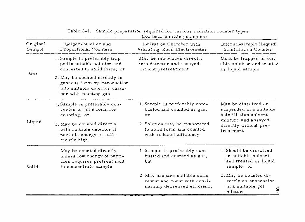
Table 8 -1. Sample preparation required for various radiation counter types (for beta - emitting samples)
Original Sample
Geiger -Mueller and Proportional Counters
Ionization Chamber with Internal -sample (Liquid) Vibrating -Reed Electrometer Scintillation Counter
Gas
1. Sample is preferably trap- ped in suitable solution and converted to solid form, or
2. May be counted directly in gaseous form by introduction into suitable detector cham- ber with counting gas
May be introduced directly into detector and assayed without pretreatment
Must be trapped in suit- able solution and treated as liquid sample
Liquid
1. Sample is preferably con- verted to solid form for counting, or
2. May be counted directly with suitable detector if particle energy is suffi- ciently high
1. Sample is preferably corn - busted and counted as gas, or
2. Solution may be evaporated to solid form and counted with reduced efficiency
May be dissolved or suspended in a suitable scintillation solvent mixture and assayed directly without pre- treatment
May be counted directly unless low energy of parti- cles requires pretreatment
Solid to concentrate sample
1. Sample is preferably corn - busted and counted as gas, but
2. May prepare suitable solid mount and count with consi- derably decreased efficiency
1 Should be dissolved in suitable solvent and treated as liquid sample, or
2. May be counted di- rectly as suspension in a suitable gel mixture
N lJ1 G.)
254 importance of the assay method, a major portion of this chapter will
be devoted to the preparation of liquid scintillation counting samples.
The reader will find an extensive bibliography on this topic at the end
of the chapter. Such a lengthy list of references was felt necessary
in view of the present state of the literature in this field.
A number of papers may be found which survey sample pre-
paration methods for a specific isotope of importance. Those which
pertain to liquid scintillation assay will be cited later, but those deal-
ing with preparation of samples for the other detection methods
should be noted here. The general preparation of C14 counting sam-
ples has been most widely described (3, 11, 16, 19, 20, 37, 40, 48), of
these references the classic work of Calvin, et al. , deserves special
notice. Somewhat less general consideration has been given to Fe59
(42), 1131 (41) S35 (18, 20), H3 (60), and Ca45 (15).
B. Conversion of Original Sample to Suitable Counting Form
Pretreatment of biological samples prior to radioactivity
assay is normally concerned with measures to reduce bulk and pro-
duce a more uniform material. Depending on the assay method to be
used, it may be necessary to convert the sample to a more suitable
physical state. It may further be desirable to convert the chemical
form of the isotope to one more suitable for both radioactivity
255
measurement and parallel chemical analysis. This is often the case
with liquid scintillation samples, where the original sample form is
a severe quenching agent, either due to its color or molecular struc-
ture. Frequently it is necessary to isolate an active compound from
a large volume of sample material (tissue, feces, blood, etc:).
The specific treatment employed for a given sample_ is depend-
ent on its original form, particle energy, and the desired method of
detection. It should be emphasized, however, that the various sam-
ple conversion methods are not unique to any given assay method.
For example, C1402 produced by Sch5niger flask oxidation can be
just as well assayed directly in an ion chamber -electrometer system,
or trapped in NaOH, converted to BaCO3 and counted on a planchet
using a G -M detector, or yet trapped in "Hyamine" and assayed by a
liquid scintillation counter. A wide variety of standard chemical me-
thods are available to allow the conversion of biological samples to a"
more suitable form for assay. Since these are well described in the
analytical chemical literature, emphasis will be placed here on adap-
tations specific to radioactive sample conversions.
1. Ashing methods
When the radionuclide to be assayed is a metallic or mineral
component, ashing of the sample is often the most practical method
256
of concentration. This removal of the organic components may be
accomplished by either dry or wet ashing. Since the dry ashing
process produces a friable residue and is often accompanied by vola-
tilization or fusion of the sample with the crucible, wet ashing is
generally preferred. A number of wet ashing procedures have been
described, but most are variations of the conventional Kjeldahl me-
thod. Various combinations of nitric, sulfuric, hydrochloric, or
perchloric acid and hydrogen peroxide have been successfully em-
ployed. Wet ashing is particularly applicable to blood or tissue con-
taining radioiron (98, 147).
Animal tissues may be converted to a homogeneous solution
for assay as a liquid by various forms of pseudo wet ashing. The
use of formamide to effect such solution has been pointed out by
several investigators (40, 53, 59). An entire animal or organ is
homogenized or cut up with scissors and placed in hot formamide.
Complete solution of all but bone results in 1 - 2 hours.
2. Combustion methods
Sample material containing the low energy beta emitters C14
or H3 usually requires complete oxidation. The tritium is recovered
as water. The C14O2 produced may be assayed in the gaseous state
or trapped in an alkaline solution prior to conversion to a suitable

257
counting form for other types of activity measurement. Where the
samples are to be assayed in a solid form, such treatment is essen-
tial to concentrate the isotopic material and reduce sample self -
absorption. For assay by the liquid scintillation method, complete
oxidation usually has the beneficial effects of improving sample solu-
bility in the solvent and reducing quenching. Jeffay has reviewed
succintly the various oxidation techniques for preparation of liquid
scintillation samples (141).
a. Wet combustion: Several wet combustion methods have
been employed, of which variations of the Van Slyke -Folch have been
the most common. The apparatus for one previously undescribed
modification is illustrated in Figure 8 -1. In this procedure the C14-
containing sample is placed in flask A and the NaOH absorbant solu-
tion in flask B. The system is assembled, evacuated, and sealed
off. A mixture of fuming sulfuric acid, phosphoric acid, and chro-
mic trioxide is introduced through stopcock C. Flask A is then heat-
ed cautiously with a low flame to promote the combustion and the
C1402 generated is allowed to come to equilibrium with the absorb-
ant (approximately 1/2 hour). Subsequent precipitation with BaC12-
NH4C1 solution yields BaC1403, which is then collected by filtration
or centrifugation for planchet mounting. Problems with this proce-
dure arise from the production of volatile byproducts (especially
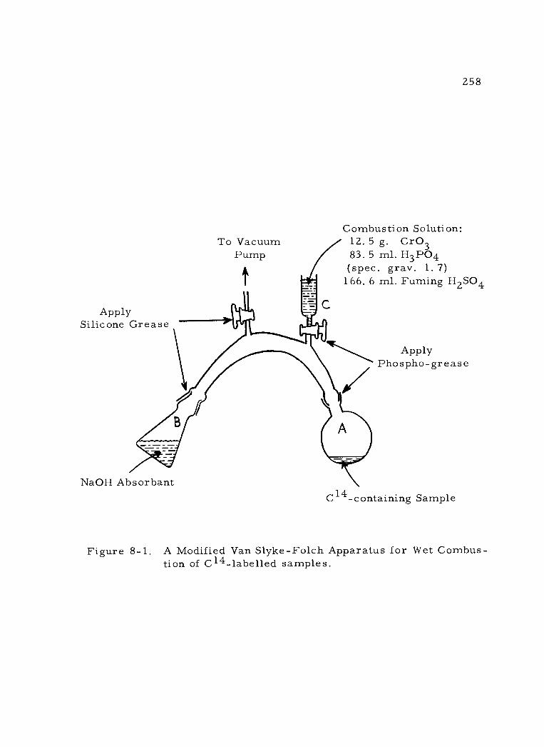
Apply Silicone Grease
258
Combustion Solution: To Vacuum 12.5 g. Cr03
Pump 83.5 ml. H3 PO4
t (spec. gray. 1.7)
= 166. 6 ml. Fuming H2SO4
C
/ NaOH Absorbant
Apply Phospho - grease
C14-containing Sample
Figure 8 -1. A Modified Van Slyke -Folch Apparatus for Wet Combus- tion of C14- labelled samples.
259
aldehydes) and the variability of heating required for different sample
types. Other modifications of this method have been made to allow
rapid and routine sample preparation (14, 31). The method is not
useful for tritium.
The persulfate oxidation of carbon compounds is also quite
convenient (2,29). Samples, however, must be soluble in water,
which somewhat restricts its application. This method uses a closed
Erlenmeyer flask with a center well containing a carbon dioxide ab-
sorbant. The aqueous solution of the sample is placed around the
well, and sulfuric acid and solid potassium persulfate added. Silver
nitrate solution is dropped in to catalyze the reaction and the flask
capped immediately. Heating accelerates the oxidation and the CO2
produced diffuses to the absorbant well. Unfortunately, volatile
intermediate products (such as acetaldehyde) may also diffuse into
the center well, giving unpredictable results.
Belcher (76) has proposed wet oxidation of tritium - labelled
samples using a nitric- perchloric acid mixture. The resultant tri-
tiated water is distilled off and the distillate assayed using a liquid
scintillation counter.
b. Dry combustion: Procedures involving dry combustion in
an oxygen atmosphere are of particular value in preparing C14 and
tritium samples for liquid scintillation or ion chamber assay. The

260
classical technique of oxidizing the sample by means of an inorganic
oxidizing agent (CuO or NiO) in a combustion furnace with a flow of
oxygen has been adapted by Peets, et al. (168), for liquid scintilla-
tion counting. The tritiated water produced is trapped as ice in a
dry ice container, while the C14O2 is taken up in a suitable alkaline
absorbing solution. Recoveries of about 96 percent were obtained
from samples of up to 1.5 grams (180, p. 185 -191). Others have
adapted this combustion train method for preparation of samples for
ion chamber (4) and proportional counter assay (26).
In an alternative method of dry oxidation the sample and oxide
catalyst are placed in a Pyrex or Vycor tube, which is then sealed
and heated. The sealed tube is subsequently broken and the oxidation
products removed by vacuum line transfer to either an absorbing solu-
tion or directly into an internal sample detector. Wilzbach, et al.
(62 -64), have employed this method for gas assay in an ion chamber,
and Buchanan and Corcoran (7) have used it with a proportional de-
tector, while Steel (192) and Jacobson, et al. (137), have adapted it
to liquid scintillation assay of tritium. The major disadvantages of
this procedure are the small sample size that can be accomodated
(less than 25 mg) and the time involved per sample.
The Schöniger oxygen flask combustion originally proposed
for halogen determinations (52) has been applied by Kallberer and
261
Rutschmann (142) to liquid scintillation sample preparation. In this
procedure the sample material is placed in a cellophane or filter
paper bag and dried. The bag is suspended in a platinum basket
which is attached to an ignition head. This assembly is placed in a
gas tight flask containing an oxygen atmosphere. When current is
applied, the oxidation takes place rapidly (180, p. 185 -191). Com-
bustion products may be frozen out (H3), or trapped by a suitable
absorbant introduced through a side arm (C14). MacDonald (35) has
reviewed this method and its specific uses for C14 sample prepara-
tion. A major problem of the Schöniger flask technique is the dan-
ger of explosion if even traces of organic solvents are present in the
flask. Martin and Harrison (157) have attempted to circumvent this
problem by designing the top of the flask to act as a safety outlet in
case of excessive internal pressure. A modification of this techni-
que achieves ignition by focusing an external infra -red heat lamp on
the sample wrapped in black paper (163). Because of the simultane-
ous combustion of the cellophane or paper bag with the sample, speci-
fic activity of the sample cannot be determined by this method. Only
total sample activity is measurable. Sample size is limited to less
than 300 mg according to Kelly, et al. (144). In addition, uneven
combustion in the flask is undetectable.
The Parr oxygen bomb (commonly used in calorimetry) offers
the advantage of allowing specific activity determination on larger
262
liquid or tissue samples (39) and has been used on even such volatile
compounds as acetone. This metal bomb is filled with up to one
gram of lyophilized tissue sample and oxygen at 25 atmospheres
pressure. Ignition produces rapid combustion and the combustion
products are removed through a collecting train. Sheppard and
Rodegker (180, p. 192 -194, 189) have reported detection of as little
as 4 x 10 -4µc of tritium and 1 x 10 -4µc of carbon -14 in three grams
of fresh tissue.
3. Miscellaneous methods
With certain samples the labelled compounds may be chemi-
cally extracted without the necessity of ashing or oxidation. Schulze
and Long (184) have reported extraction by ultrasonic treatment of
the sample directly in the liquid scintillation counting vial. Tritiated
water samples may be prepared from biological fluids (plasma,
urine) by distillation. Simpson and Greening (56) have investigated
the magnitude of isotopic effect on such distillations of tritiated water
from urine and found it negligible.
C. Assay of Samples in Various Counting Forms
The three physical states of counting samples (gaseous, li-
quid, solid) can be assayed by a variety of detectors, with, of

263
course, different counting efficiencies. In general, solid counting
samples require the most careful attention to mounting in order to
ensure reproducibility of results. The preparation of counting sam-
ples for liquid scintillation assay has been singled out for more ex-
tensive discussion because it involves the unique feature of actually
introducing the sample into the fluor medium.
1. Assay of gaseous counting samples
Samples that are to be assayed in a gaseous form are usually
introduced directly into the detector (ion chamber, G -M detector, or
proportional detector) following their preparation from the original
biological material (180, p. 167 -184). However, vacuum transfer
technique is involved in this operation. The significant advantage of
gas counting is that self -absorption is largely circumvented. Thus,
gas counting is largely restricted to the low energy beta -emitters
C14 H3 and S35. These nuclides are most commonly assayed in the
chemical form of CO2 or C2H2, H2 or CH4, and SO2 or H2S, respec-
tively. Wilzbach and Sykes (64) have described methods of C14O 2
activity determinations in ion chambers, while Eidenoff (17) has dis-
cussed G -M assay of the same compound. Although counting effi-
ciencies may be reasonably high for these isotopes, compared to
other assay methods, the overall sample preparation is rather

264
tedious and time consuming. It is necessary to calibrate gas coun-
ters with standard gaseous sources of the same nuclide that is being
assayed. In certain circumstances it is possible to make continuous
flow measurements on gaseous samples (see Experiment B), as from
respiring animals or gas chromatography effluent streams. Such a
procedure eliminates sample preparation entirely.
2. Assay of liquid counting samples
If a liquid sample is to be assayed directly, a minimum of
further sample preparation is required. Except for the internal -
sample scintillation counting method (described on pages 271 -286),
liquid sample counting is largely restricted to gamma- and high en-
ergy beta -emitters. G -M tubes of specialized design are available
(see Figure 4 -7 D, E, F) for the latter sample type. McAuliffe (33)
describes typical procedures for G -M counting of P32 solutions.
Because of the low efficiency of ionization -type detectors for
gamma photons, a NaI (T1) scintillation detector is normally em-
ployed for gamma ray assay. Well -type scintillation detectors com-
bine high counting efficiency with simplicity of sample preparation
for gamma- emitting biological samples. The homogeneous liquid
sample need only be poured into a counting vial and placed in the
crystal well. Experiments C and D in Part Three illustrate such an
265
application for the assay of Fe59 in whole blood and Na22 in water,
respectively. It is essential for comparative purposes that standard
volumes of sample be used from assay to assay, since detection effi-
ciency is inversely related to counting sample volume and decreases
rapidly as the sample volume exceed the well capacity. Likewise,
calibration of such detectors must be done with both the same nu-
clide and volume as the samples to be assayed. As in the case of
gas counters, it is possible to arrange these detectors to make con-
tinuous flow measurements on liquid samples, subject to the fore-
going limitation on emitter type. Methods for assay of stationary
liquid samples in a coiled tubing mounted against the solid fluor have
also been described (43, 54).
3. Assay of solid counting samples
Solid counting samples are satisfactory for most radioiso-
topes and have the advantage of being more easily handled and stored
than the other types. In general, two types of solid counting samples
are utilized -- those on paper chromatograms and those mounted on
planchets. In turn, solid samples of these types may be assayed by
ion chamber -electrometer systems, G -M counters, proportional
counters, or external - sample scintillation counters. As will be seen
later in the chapter, solid samples may also be assayed in a
266
heterogeneous counting system using a liquid scintillation counter.
a. Preparation of planchet mounts: Typically, a solid
sample is mounted on a backing material in a deposit of reasonably
uniform thickness and area. The more commonly employed backing
materials are aluminum, copper, stainless steel and glass, in the
form of flat or cupped planchets, or fritted filter plates. These ma-
terials vary in their resistance to chemical attack and must be care-
fully selected with respect to the chemical form of the counting sam-
ple. Furthermore, since backscattering of beta particles (see
Chapter 9) is related to the density of the backing material, it is
important to use the same type of material throughout an experiment
when comparison of counting data is to be made.
The requirement of preparing counting samples of uniform
thickness is most stringent when one is dealing with low energy beta -
emitters, since self- absorption in solid sources of such nuclides is
a significant factor. A number of generally applicable techniques
have been developed over the years to produce counting samples of
uniform thickness. Those most commonly used will be discussed
briefly. An excellent review of these techniques is found in the
Nuclear- Chicago Technical Bulletins 7 and 7B (21 -22).
(1) Direct evaporation from solution: Perhaps the simplest
means of converting a dissolved sample to a solid counting source is
267
by direct evaporation of the solvent (usually water or alcohol). The
procedure consists of pipetting the sample solution, or an aliquot of
it, onto a planchet and gently evaporating it to dryness under a heat
lamp. Accuracy in pipetting is a major factor in this technique. A
micro transfer pipette is normally used. It is somewhat difficult to
secure reproducible sample thicknesses by the evaporation technique
and this factor limits its application. A number of refinements to
improve uniformity of sample deposit have been developed, such as
the use of wetting agents on the planchet surface, addition of thin
sheets of absorbent material (lens tissue) to the bottom of the cupped
planchets, the use of dilute agar solutions (12, 25, 34), and the rota-
tion of the mount during evaporation.
(2) Filtration of precipitates: Larger sample amounts than
can be easily secured by direct evaporation are obtainable from sus-
pensions of precipitates, such as BaC1403. Direct filtration of the
suspension leaving the precipitate as a uniform layer on the filter
medium is the simplest procedure. Filter paper or fritted disks are
commonly used for this purpose and subsequently serve as the source
mount (1,5,44). The importance of crystal size for BaC1403 has
been investigated by Regier (46), while Shirley, et al. (55), have
compared the effect of oxalate vs. carbonate precipitates of Ca45
on reproducibility. When filter paper is used, there is some

268
difficulty in securing reproducible results due to variable paper tex-
ture and damage to the thin sample layer when it is subsequently
transferred to a mounting block and dried. With fritted glass (50)
or sintered metal disks, this problem is minimized, but their cost
is such that it is not practical to hold large numbers of samples for
permanent reference. The use of Millipore filters has been suggest-
ed by Jervis (27). Brunner and Jernberg (6) have proposed a centri-
fugal filter assembly for mounting Ca45 and S35 precipitates.
(3) Settling or centrifugation of slurries: Precipitates that
have been separated from excess solvent by centrifugation and decan-
tation may be mounted in slurry form by two different techniques.
The precipitate may be resuspended in a volatile solvent and poured
into a cup planchet. Slow drying of the slurry with occasional tap-
ping produces a remarkably uniform sample layer. Although this
technique gives good reproducibility, it is tedious. Burr and Marcia
(8) have used a screw -press to produce a smooth, flat surface with
BaC14O3 mounts. Alternately, the resuspended slurry may be cen-
trifuged again using an arrangement whereby a removable cupped
planchet serves as the false bottom of the centrifuge tube. Such ap-
paratus is commercially available. Following centrifugation, the
solvent is decanted and the planchet removed from the tube and dried
before counting (24, 30). This is a relatively simple procedure and
269
can be readily used with large numbers of samples. It gives reason-
ably good reproducibility (see Experiment 6, Section C).
(4) Mounting dry powdered samples: When a sample consists
of ash or dried soil, it may be most convenient to weigh it directly
into a cup planchet. The particles may be compressed (36) or the
planchet tapped to produce a more even distribution, An example of
this method with Zn65- labelled plant tissues is seen in Experiment E.
It is highly desirable to treat such a mounted sample with a binder,
such as a solution of collodion, to prevent disturbing or spilling of
the deposit in handling. In general this method is not applicable to
samples containing low energy beta -emitters.
(5). Electroplating: Uniform and thin films of many metals
may be prepared by electrodeposition. The sample is usually plated
in elemental form which allows a maximal specific activity to be at-
tained. The thin uniform films obtainable have the twin advantages of
minimizing self -absorption and ensuring reproducibility. Unfortun-
ately, the procedure is quite laborious and time consuming and is
limited to metallic ions.
b. Radiochromatogram scanning: In view of the widespread
use of paper chromatography to separate complex mixtures of label-
ed compounds, it is not surprising to find that much effort has been
expended on developing methods of assaying radiochromatograms
270
(23, 65 -66). In general, paper chromatograms containing C14 S35,
or, to a lesser extent, H3 lend themselves fairly well to direct assay,
despite the problem of self -absorption (see Experiment A). Since the
typical paper strip chromatogram may have a series of active spots
at varying distances from the point of origin, it is highly desirable
to have some means of scanning the length of the strip and recording
both the extent of the activity and its location.
Many types of radiochromatogram scanners have been des-
cribed (13, 28, 32, 38, 45, 47, 51, 57) and several models are com-
mercially available. Basically these consist of a detector (usually
a windowless G -M tube), a strip chart recorder, and a drive mech-
anism to move the chromatogram past the collimated detector at a
fixed speed. Unfortunately, the counting efficiency of such systems
is often poor and the relation between chart recording and chromato-
gram strip inaccurate. To improve counting efficiency several com-
mercially available counters use a pair of windowless G -M detectors
mounted end -to -end, thus attaining nearly 4 Tr geometry. Alterna-
tively, the strip may be cut into serial sections and these assayed
individually. Such a procedure using liquid scintillation counting is
described on page 286 . Svendsen (58) has suggested a method of
eluting the spots onto planchets and counting as solid samples.
271
D. Preparation and Assay of Liquid Scintillation Counting Samples
1. Basic considerations in the choice of scintillation solutions
a. Sample solubility: The unique feature of liquid scintilla-
tion counting is that the sample is in intimate contact with the scin-
tillation solution. The components of such solutions have been dis-
cussed previously (see Chapter 6). Clearly the best contact between
sample and fluor is achieved when both are dissolved in the same
solvent mixture. Unfortunately, simple solution is not always feasi-
ble for many biological samples. A variety of alternative methods
have been developed to improve sample solubility or at least to bring
the sample material and the scintillation solutions into defined proxi-
mity. The concoction of suitable scintillation solutions has taken
place on a rather empirical basis as a result of these factors and
the wide variety of biological samples encountered. Several general
references with regard to the preparation of liquid scintillation count-
ing samples might be cited (77, 95, 110, 136, 180), of which the review
by Funt and the Nuclear- Chicago Technical Bulletin No. 11 are parti-
cularly recommended.
b. Quenching: A second technical problem affecting the
choice of a suitable scintillation solution is quenching. Quenching is

272
commonly caused by the dissolved sample, and is a consequence of
the sample being polar in nature or colored. Color quenching may
be avoided by using pretreatment procedures (adsorption or combus-
tion) which decolorize the original biological sample. Alternatively,
Fales (100) suggests direct addition of ethanolic sodium borohydride
solution to the sample in the counting vial to effect decoloration.
Chemical quenching can often be reduced by addition of naphthalene
to the scintillation solution. The extent of quenching should be rou-
tinely determined as discussed in Chapter 6.
c. Homogeneous vs. heterogeneous counting systems: In
cases where the sample is, or can be made soluble in the fluor solu-
tion, a homogeneous counting system may be used. Where this is
not possible or solution leads to excessive quenching, the sample and
the scintillation solution may still be brought into intimate contact by
various means in a heterogeneous system. In view of the diversity
of sample types that may be assayed by liquid scintillation counting,
it will be evident that there is no single scintillation solution suitable
for all samples. Of course, some fluor solutions do have wider ap-
plication than others. In the remainder of this chapter the attempt
will be made to point out generally successful means of incorporating
various sample types into fluor solutions and to list in tabular form
many of the liquid scintillation solutions that have been proposed.
273
These tables are presented as a guide to the choice of a suitable
scintillation solution, but not as a substitute for the discussion in the
references cited, or individual experience.
As an added practical point it should be noted that a variety of
causes can result in fluorescence of the scintillation solution, aside
from beta particle interaction. Such fluorescence results in spuri-
ous pulses. An easily overlooked cause of such induced fluorescence
is the light from fluorescent lamps. For this reason, liquid scintil-
lation samples should be prepared in rooms illuminated by incandes-
cent lamps and the counting samples should be kept in the dark before
being assayed.
2. Homogeneous counting systems
a. Direct solution in the scintillation solvent: Where sample
solubility in the most efficient scintillation solvents (toluene, xylene,
etc. ) is no problem, the most urgent consideration is to choose a
fluor solution in which the sample will cause a minimum quenching
effect. Relatively few biological samples fall into this category,
since most are polar compounds and not readily soluble in toluene.
Table 8 -2 lists scintillation solution "recipes" that are known to con-
tribute little to pulse quenching. The sample recipes marked with an
asterisk are those used in carbon -14 dating studies. In this case
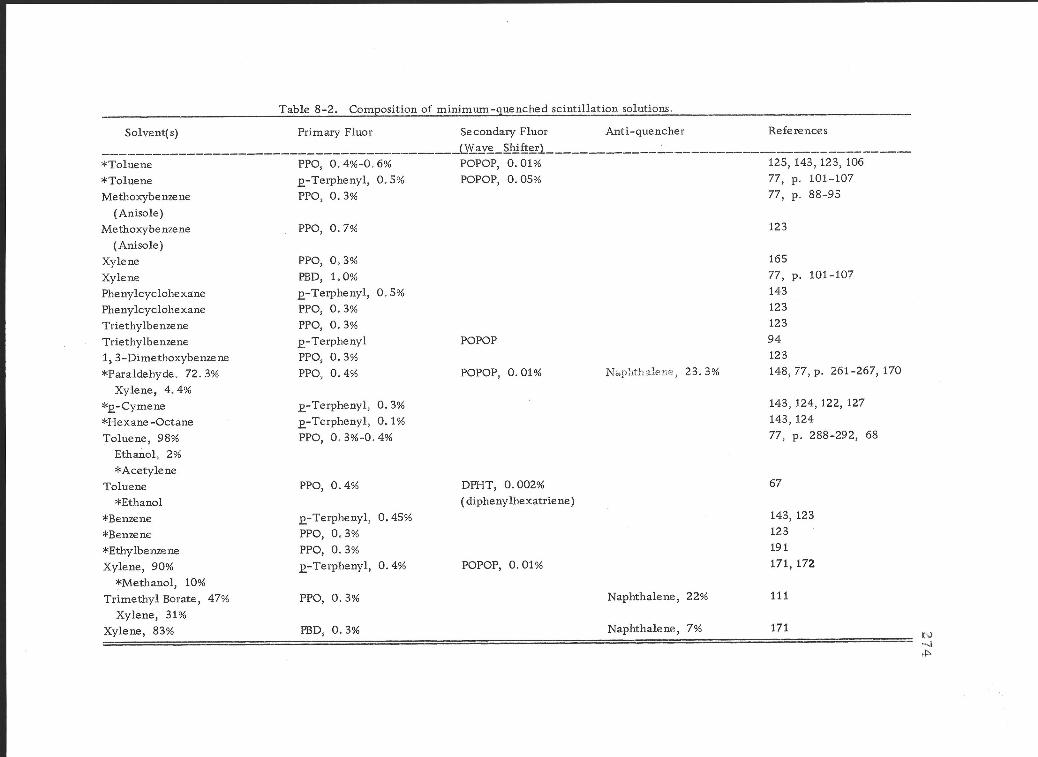
?,v 4
oNHFJ0o
eF\:
9 r.. r.-
^r;9-
I E
^i
R:j-lq
J 'l
N
J'^O
oO
O
O
. -
oo
".i- oo
s -:
+
$ (\l
co N
+
. N
^!^I
o,l N
.p.O.N
NH
Hp.H
dri
co to
-co co ro
.o od ,"idi
cr-iro * j
a H
nis.r'. ^I
ror.-d(\i(\r+ors
:f $N
t\
'+(\IotN
H
N
;a\i\HiN
sJJoleaH€F
-(oddHH
HH
ooooq,
d.
:ix(\tNddItrooddo.adrBzz
oopioo{oA
6)
.E)V
PA
T69deF
.9:E
EH
g
co",;c\tdUrJ
J:o.
zoc;
o"piooo.
orooF
eO.
6'(.)6)(,I
oooPdHo.oopooc.iIooop(d
F.
x x
xx H
x
si 1
iis 1
1(oO
O
O
O$
o o
d; ^
^ jg j
jIE
" N
xsExxE
xx E
EI
x E
**E
;s x
* ijco
N
.oo qicoco
{co<
E
E"o
$ 9.o.o
o co
(o
;f.d ;
-:f,.'.f;a E
E.
cj EaaE
o ci
^o^-o^^oo,oo^'^oo'F
o o'
o'o'r:o'o'FO
.o trF
o O
t-O
Qt-.. I
OtirE
E
eE'tuE
tltt tutue ft
tuHfrA
r &
H
*!o al--
-.5
!l! H
rr')l&
.l=l O
O
FH
I' a
E giE
B'
x (d!o" a
s =jg I
II
ss Hn
-i
r # gc$a$nF$$F
illn} }iFs F
s s $AE
ilf
EotIq(d
o.c6)o(r)
275
maximum detection efficiency is achieved by adding the sample in the
same chemical form as the solvent. This usually involves elaborate
chemical or biological syntheses starting with C14O2. The advent of
this technique made possible a considerable backward extension of
the period of time that could be accurately measured by the C14 -
dating method. Several reviews of the procedures involved are avail-
able (77, p. 129 -134 and p. 261 -267, 114, 124, 171).
b. Indirect solution in the scintillation solvent: In general,
biological samples are not soluble in toluene, the most efficient scin-
tillation solvent in common use. Thus, an indirect approach must
be taken to achieve a homogeneous sample -fluor solution (176). One
approach is to employ a mixture of solvents that will accommodate
small quantities of aqueous solutions. Inevitably, this increases
quenching and reduces counting efficiency. The mere addition of
ethanol to the common toluene solvent results in a mixture that can
hold up to three percent of aqueous sample material in solution.
Dioxane (101), as a solvent, allows the presence of much larger per-
centages of water (up to 29 percent), although it is less efficient in
energy transfer than toluene. Dioxane solutions usually require the
addition of naphthalene as an anti - quenching agent. Dioxane has the
additional disadvantage of a relatively high freezing point ( +12° C)
and often needs the addition of an antifreeze component (150).
276
Table 8 -3 lists "recipes" for scintillation solutions with varying de-
grees of water tolerance. These solutions have particular signifi-
cance in tritium counting, since it is usually assayed as tritiated
water (90, 102, 137). In an attempt to avoid the disadvantage of di-
oxane as a solvent, Avinur and Nir (69) have used an acid catalyzed
tritium exchange between tritiated water (THO) and toluene. Much
improved counting efficiency resulted, but the method is quite time
consuming.
The measurement of C14O2 by the liquid scintillation method
poses the problem of finding a suitable absorption medium. This
trapping agent should combine with CO2 to produce a toluene - soluble
salt with minimal quenching effect. The first such trapping agent
proposed was a methanolic or ethanolic solution of the hydroxide of
Hyamine 10 -X (Rohm and Hass, Inc. ) (167). The original technique
was later refined by Frederickson and Ono (105). Rapkin has review-
ed the uses of this substance in liquid scintillation counting (174).
": Hyamine" continues to be the most widely used trapping agent for
C 1402. However, it suffers from the disadvantages of a relatively
high cost, requiring somewhat tedious preparation from the original
crystalline material (77, p. 123 -125), and displays a significant
quenching effect.
Other C14O2 trapping agents have been suggested. Primene
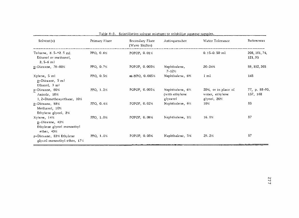
Table 8 -3. Scintillation solvent mixtures to solubilize aqueous samples.
Solvent(s) Primary Fluor Secondary Fluor (Wave Shifter)
Anti -quencher Water Tolerance References
Toluene, 8. 5 -?.2. 5 ml PPO, 0.6% POPOP, 0.01% 0.15-0.50 ml 208, 161, 74,
Ethanol or methanol, 2. 5 -6 ml
p- Dioxane, 76 -80% PPO, 0.7% POPOP, 0.005% Naphthalene, 7 -12%
20 -24%
121, 93
89, 112, 203
Xylene, 5 ml PPO, 0.5% of.-NPO, 0.005% Naphthalene, 6% 1 ml 145
R- Dioxane, 5 ml Ethanol, 3 ml
p- Dioxane, 60% PPO, 1.2% POPOP, 0.005% Naphthalene, 6% 20 %, or in place of 77, p. 88 -95, Anisole, 10%
1, 2- Dimethoxyethane, 10%
(with ethylene glycerol
water, ethylene glycol, 20%
137, 168
R- Dioxane, 88% PPO, 0.4% POPOP, 0.02% Naphthalene, 6% 10% 83
Methanol, 10%
Ethylene glycol, 2%
Xylene, 14% PPO, 1.0% POPOP, 0.08% Naphthalene, 8% 16.1% 87
R- Dioxane, 43%
Ethylene glycol monoethyl ether, 43%
p- Dioxane, 83% Ethylene PPO, 1.0% POPOP, 0.05% Naphthalene, 5% 29.2% 87
glycol monoethyl ether, 17%
278
81 -R (Rohm and Hass, Inc.) is less costly, may be used directly as
supplied, and shows little quenching effect in moderate concentra-
tions (164). Unfortunately, it does not absorb CO2 as readily as
"Hyamine" and requires the use of multiple traps. Ethanolamine
is relatively inexpensive and shows little quenching effect (180,
p. 113 -114). It, however, requires the use of ethylene glycol mono -
methyl ether (a rather toxic compound) or ethanol to facilitate solu-
bility of the resulting ethanolamine carbonate in toluene. Ethylene
diamine is also usable, but can accommodate only limited amounts
of CO2 (up to 1 mM). Phenylethylamine has much greater trapping
capacity and less quenching effect than "Hyamine ". Rapkin (177) has
reviewed in detail the various C140 trapping agents proposed. The
first portion of Table 8 -4 lists several common "recipes" used in
solution counting of C140 2.
The method of Gordon, et al. (118), for liquid scintillation
assay of H2S35 should also be mentioned. Finding "Hyamine" an un-
satisfactory trapping agent, they modified the caps of their counting
vials to allow direct injection of the gas through a silicone rubber
insert into the air space over a toluene- PPO -POPOP solution. They
found very linear counting results with increasing quantities of
H2S35. It is suggested that this method may have application to other
gaseous samples.
279
In an attempt to overcome the insolubility of most metallic
ions in the organic scintillation solvents, a variety of specific solu-
bilizing agents have been investigated (99, 135). In general, these
act by either forming an organic complex with the ions, or convert-
ing them to the salt of an organic acid. To date, the best organic
complexing agents to be used with liquid scintillation systems are
the acidic esters of orthophosphoric acid, i. e. , dibutyl phosphate,
tributyl phosphate, dioctyl phosphate, etc. However, other organic
complexing agents have been used in specific cases to good advantage.
Metallic salts of 2- ethylhexanoic acid (octoic acid) are readily solu-
ble in toluene and have high scintillation efficiencies even at quite
high concentrations. Table 8 -4 lists solvent systems and binding
agents useful in incorporating a large variety of inorganic ions into
a homogeneous counting system.
Considerable attention has been directed in recent years to-
ward the development of techniques allowing liquid scintillation
counting of labelled whole tissues, blood, and urine with minimal
sample pretreatment (77, p. 223 -229, 85, 132). "Hyamine" has
been used to solubilize animal tissues (71, 86), bacterial cell debris
(120), and blood serum (91, 199). The problems of poor solubility
and color quenching have plagued such efforts, but decreased count-
ing efficiency can sometimes be tolerated as the price for more
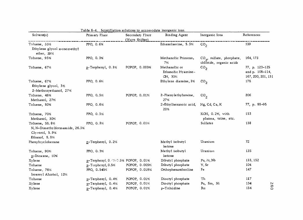
Table 8 -4. Scintillation solutions to accomodate inorganic ions. Solvent(s) Primary Fluor Secondary Fluor
(Wave Shifter_ Binding Agent Inorganic Ions References
Toluene, 55% PPO, 0.6% Ethanolamine, 5.5% CO2 139
Ethylene glycol monomethyl ether, 39%
Toluene, 93% PPO, 0.3% Methanolic Primene, 7%
CO2, sulfate, phosphate, chloride, organic acids
164, 173
Toluene, 67% p-Terphenyl, 0.3% POPOP, 0.003% Methanolic or CO2 77, p. 123 -125 Ethanolic Hyamine- and p. 108 -114, OH, 33% 167, 200, 201, 131
Toluene, 67% PPO, 0.6% Ethylene diamine, 3% CO2 178
Ethylene glycol, 3%
2- Methoxyethanol, 27%
Toluene, 46%
Methanol, 27%
PPO, 0.5% POPOP, 0.01% 2- Phenylethylamine, 27%
CO2 206
Toluene, 80% PPO, 0.6% 2- Ethylhexanoic acid, 20%
Hg, Cd, Ca, K 77, p. 88-95
Toluene, 70%
Methanol, 30%
PPO, 0. 3% KOH, 0.2 %, with plasma, urine, etc.
115
Toluene, 58.8% PPO, 0.3% POPOP, 0.01% Sulfates 138
N, N- Dimethylformamide, 26.5%
Glycerol, 5.9% Ethanol, 8.8%
Phenylcyclohexane p-Terphenyl, 0.2% Methyl isobutyl ketone
Uranium 72
Toluene, 90%
p- Dioxane, 10%
PPO, 0.3% Methyl isobutyl ketone
Uranium 135
Xylene p-Terphenyl, 0. '%-0. 5% POPOP, 0.01% Dibutyl phosphate Pu, Zr, Nb 133, 152
Toluene p-Terphenyl, 0.5% POPOP, 0.005% Dibutyl phosphate Y, Sr 104
Toluene, 78% PPO, 0.545% POPOP, 0.018% Orthophenanthroline Fe 147
Isoamyl Alcohol, 12%
Toluene 2-Terphenyl, 0.4% POPOP, 0.01% Dioctyl phosphate Th 117
Xylene 2-Terphenyl, 0.4% POPOP, 0.01% Dioctyl phosphate Pu, Sm, Ni 134 oo
Xylene p-Terphenyl, 0.4% POPOP, 0.01% p- Toluidine Ru 134 O ry
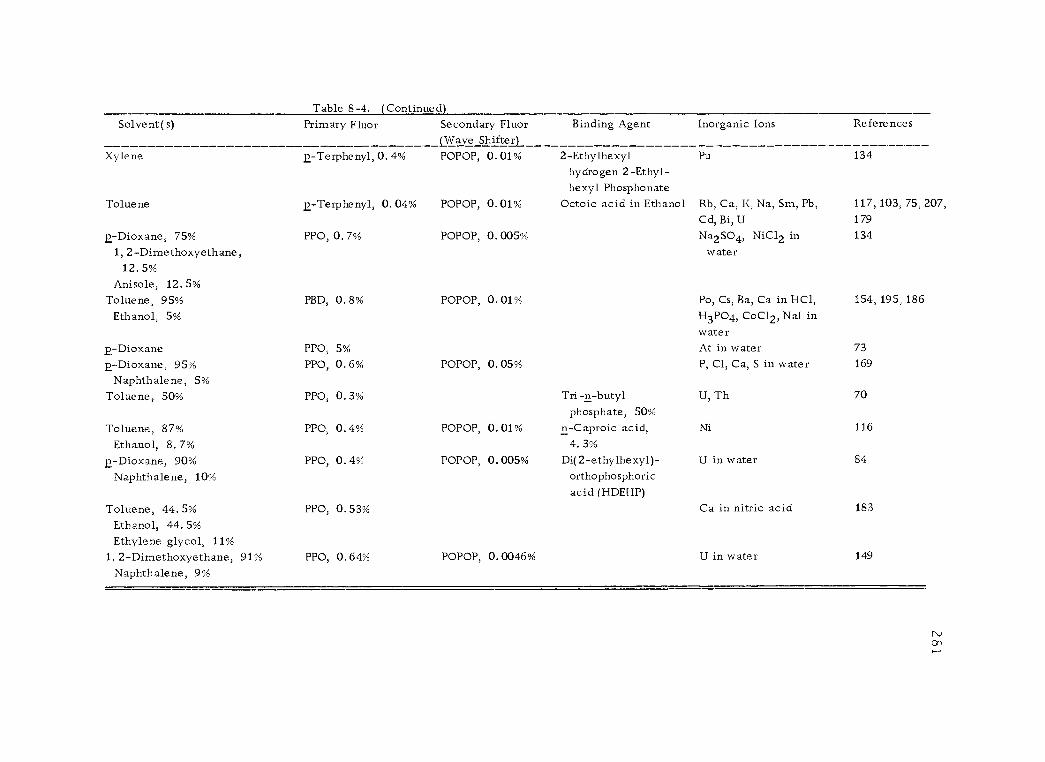
Table 8 -4. (Continued) Solvent(s) Primary Fluor Secondary Fluor Binding Agent Inorganic Ions References
(Wave Shifter)._ Xylene p- Terphenyl, 0. 4% POPOP, 0.01% 2- Ethylhexyl
hydrogen 2- Ethyl- hexyl Phosphonate
Pu 134
Toluene 2-Terphenyl, 0.04% POPOP, 0.01% Octoic acid in Ethanol Rb, Ca, K, Na, Sm, Pb, 117, 103, 75, 207,
Cd, Bi, U 179
p- Dioxane, 75%
1, 2- Dimethoxyethane, 12.5%
PPO, 0.7% POPOP, 0.005% Na2SO4, NiC12 in water
134
Anisole, 12.5% Toluene, 95%
Ethanol, 5%
PBD, 0.8% POPOP, 0.01% Po, Cs, Ba, Ca in HC1,
H3PO4, CoC12, NaI in water
154, 195, 186
p- Dioxane PPO, 5% At in water 73
p- Dioxane, 95% PPO, 0.6% POPOP, 0.05% P, Cl, Ca, S in water 169
Naphthalene, 5%
Toluene, 50% PPO, 0.3% Tri -n -butyl phosphate, 50%
U, Th 70
Toluene, 87%
Ethanol, 8.7% PPO, 0.4% POPOP, 0.01% n- Caproic acid,
4. 3%
Ni 116
p- Dioxane, 90%
Naphthalene, 10%
PPO, 0.4% POPOP, 0.005% Di(2- ethylhexyl)- orthophosphoric acid (HDEHP)
U in water 84
Toluene, 44.5% PPO. 0.53% Ca in nitric acid 183
Ethanol, 44.5% Ethylene glycol, 11%
1, 2- Dimethoxyethane, 91% PPO, 0.64% POPOP, 0.0046% U in water 149
Naphthalene, 9%
282
simplified sample preparation. The direct liquid scintillation assay
of untreated urine samples containing tritium has been attempted (89,
146, 161). However, decolorizing and centrifuging are usually ne-
cessary. Dioxane is typically used as the solvent in such cases.
Such urine assays are of particular importance as a health physics
measure for investigators using high levels of certain tritiated com-
pounds.
3. Heterogeneous counting systems
Radioactive samples which cannot be dissolved in some suit-
able solvent system may still be assayed by the liquid scintillation
process in a heterogeneous system. The samples may be suspended,
either by shaking or in a gel, or they may be dried on filter paper and
the paper strips placed in a fluor solution. Rapkin (175) has reviewed
these systems in detail. In addition, an aqueous sample may be intro-
duced into a counting vial containing a solid, insoluble fluor (anthra-
cene) as described in Chapter 6.
a. Gel suspension counting: Hayes, et al. (126), reported a
technique involving the liquid scintillation counting of finely ground
sample material that was suspended by agitation immediately before
assay. The technique was applied to a wide variety of sample materi-
als, but had the disadvantages of requiring multiple counts of the same

283
sample and lacking precision. The technique is not widely used to-
day. The significant point was that the presence of opaque materials,
either as dispersed water droplets or fine white solids, did not re-
duce the counting efficiency significantly as compared to a homo-
geneous system. Self- absorption appeared to be only a minor pro-
blem, except for tritium labelled samples, when the particulate ma-
terial was finely ground.
Funt (107) was the first to propose the use of a gelling agent
to suspend particulate samples for liquid scintillation counting. He
used aluminum stearate (five percent) as the gelling agent and inject-
ed the sample material throughout the already formed gel by means
of a fine hypodermic needle. This technique proved particularly
suitable for assay of finely ground BaC 1403 (108). The importance
of gel counting is that samples that would cause severe quenching in
solution, may be counted in suspension with only minimal quenching.
It is essential, however, that the sample material be completely in-
soluble in the scintillation solvent used, lest variable counting effi-
ciencies from sample to sample result.
A modification of this technique using the gelling agent,
Thixcin (Baker Castor Oil Co. , Inc. ), was subsequently introduced
by White and Helf (205). They suggested a gel system prepared by
adding 25 grams of Thixcin to one liter of scintillator solution

284
(toluene-O. 4 percent PPO -0. 01 percent POPOP) and blending (77,
p. 96 -100, 130). The result is a pourable solution which quickly
sets to a gel. Approximately one gram of suspended material can
be supported in 20 ml of gel. This gel system has been used in as-
saying organic nitrocompounds (129), ground barium carbonate (159),
and aqueous solutions of carbon -14 and tritium compounds (188).
More recently, Ott, et al. (166) have used Cab -O -Sil M -5
(Godfrey L. Cabot, Inc. ), a pure silica of extremely fine particle
size, as a gelling agent. It is particularly advantageous since it re-
quires neither blending nor heating, can be used with either toluene
or dioxane, and forms an almost transparent gel merely by shaking
in the counting vial. Cab -O -Sil gels will support about twice as much
sample material as the same weight of Thixcin gel, and also give
higher counting efficiencies. Gordon and Wolfe (119) have used Cab-
O-Sil gels in assaying aqueous solutions (up to 6. 5 percent by vol-
ume) with quite respectable counting efficiencies, while Snyder and
Stephens (190) have used such gels to count C14- and H3 -labelled
scrapings from thin layer chromatograms. Cab- O -Sil, however,
being finely powdered silica, poses the serious health hazard of
silicosis to its users. Cab -O -Sil has also been employed to reduce
the extent of adsorption of certain polymer samples to the walls of
the counting vials, which would result in decreased counting

285
efficiency (79).
Other gelling agents have also been suggested, such as dis-
solved polystyrene and methyl methacryalate (Plexiglas).
Shakhidzhanyan, et al. (187), have used gels of the latter substance
in assaying K40- containing ash from human organs. Chemilumines-
cence is often a problem in gel suspension counting. It is best avoid-
ed by the addition of small quantities of Tween or Span to the count-
ing samples. Chemiluminescence may also result in other types of
counting samples.
b. Filter paper counting: Another effective means of liquid
scintillation counting of heterogeneous systems involves direct count-
ing of toluene -insoluble samples on filter paper. This has been ap-
plied most successfully to counting paper chromatogram sections,
but has also been used with pieces of filter paper on which samples
have been added and dried in place. Davidson (96) has reviewed the
various techniques proposed in this type of system.
A relatively crude technique has been developed in which the
filter paper carrying the dried sample is wetted with a scintillator
solution and then applied directly to the face of a photomultiplier
(109, 181, 185). The paper is rendered relatively transparent by
the wetting and can be counted with reasonable, but not very repro-
ducible efficiency.

286
Wang and Jones (202) first proposed immersing a paper chro-
matogram section directly in the vial of scintillator solution. They
obtained quite respectable counting efficiencies and the technique al-
lowed the use of automatic sample changing equipment for handling
large numbers of samples. Geiger and Wright (113) have evaluated
this technique with regard to the orientation of the paper strips in
the counting vial with respect to the photomultipliers. Loftfield and
Eigner (151) suggested that the paper strip be formed into a cylinder
which completely lines the counting vial to offset the problem of vari-
able orientation. Uniform drying of the paper strip is essential and,
as in gel counting, the sample material must be toluene -insoluble.
The method of Wang and Jones has been widely used for liquid scin-
tillation counting of paper chromatograms (82, 160, 180, p. 121-126,
197) and filter paper disks on which radioisotope samples have been
precipitated (78, 156). A recent adaptation of the technique allows
the assay of C14O2 trapped on KOH- impregnated filter paper in a
Warburg flask (88, 92).
BIBLIOGRAPHY
General Counting Sample Preparation
1. Armstrong, W. D. and Jack Schubert. Determination of radio- active carbon in solid samples. Analytical Chemistry 20:270- 271. 1948.
287
2. Baker, Nome, Harold Feinberg, and Robert Hill. Analytical procedures using a combined combustion - diffusion vessel: simple wet -combustion method suitable for routine carbon -14 analyses. Analytical Chemistry 26:1504 -1506. 1954.
3. Beamer, William H. and George J. Atchison. Quantitative tech- niques with carbon -14. Analytical Chemistry 22:303 -306. 1950.
4. Biggs, Max W. , David Kritchevsky and Martha Kirk. Assay of samples doubly labeled with radioactive hydrogen and carbon. Analytical Chemistry 24:223 -224. 1952.
5. Bloom, Ben. Filter paper support for mounting and assay of radioactive precipitates. Analytical Chemistry 28:1638. 1956.
6. Bronner, Felix and Nils A. Jernberg. Simple centrifugal filtra- tion assembly for preparation of solid samples for radioassay. Analytical Chemistry 29:462. 1957.
7. Buchanan, Donald L. and Betty J. Corcoran. Sealed tube com- bustions for the determination of carbon -14 and total carbon. Analytical Chemistry 31 :1635 -1638. 1959.
8. Burr, William W and John A. Marcia. Preparation of pressed samples for counting carbon -14- labeled compounds. Analyti- cal Chemistry 27:571. 1955.
9. Burr, William W. , Jr. and Donald S. Wiggans. Direct deter- mination of C14 and S35 in blood. The Journal of Laboratory and Clinical Medicine 48:907 -911. 1956.
10. Cahn, Arno and R. M. Lind. An improved procedure for plating uniform BaCO3 precipitates. The International Journal of Applied Radiation and Isotopes 3 :44 -45. 1958.
11. Calvin, Melvin, et al. Isotopic carbon. Techniques in its meas- urement and chemical manipulation. New York, John Wiley, 1949. 376 p.
12. Campbell, H. , H. A. Glastonbury and Margaret D. Stevenson. A direct - plating method for the assay of radioactive isotopes in aqueous and alcoholic samples. Nature 182:1100. 1958.

288
13. Carleton, F. J. and H. R. Roberts. Determination of the spe- cific activity of tritiated compounds on paper chromatograms using an automatic scanning device. The International Journal of Applied Radiation and Isotopes 10:79 -85. 1961.
14. Claycomb, Cecil K. , Tyra T. Hutchens and John T. Van Bruggen. Techniques in the use of C 14 as a tracer. I.
Apparatus and technique for wet combustion of non - volatile samples. Nucleonics 7(3):38 -41. 1950.
15. Comar, C L. , et al. Use of calcium -45 in biological studies. Nucleonics 8(3):19 -31. 1951.
16. Dauben, William G. , James C. Reid and Peter E. Yankwich. Techniques in the use of carbon 14. Analytical Chemistry 19:828-832. 1947.
17. Eidinoff, Maxwell Leigh. Measurement of radiocarbon as car- bon dioxide inside Geiger-Willer counters. Analytical Chemistry 22:529 -534. 1950.
18. Eldjarn, L. and O. Nygaard. Comments on methods in biologi- cal work with S35- labeled compounds. The Scandinavian Journal of Clinical and Laboratory Investigation 6:160 -167. 1954.
19. Evans, Ersel A. and J. L. Huston. Radiocarbon cumbustion and mounting techniques. Analytical Chemistry 24:1482- 1483. 1952.
20. Garrow, J. and E. A. Piper. A simple technique for counting milligram samples of protein labelled with 14C or35S. The Biochemical Journal 60:527-528. 1955.
21. How to prepare radioactive samples for counting on planchets -- Part 1. Des Plaines, Ill. , 1961. 4 p. (Nuclear- Chicago Technical Bulletin No. 7)
22. How to prepare radioactive samples for counting on planchets -- Part 2. Des Plaines, Ill. , 1961. 4 p. (Nuclear- Chicago Technical Bulletin No. 7B)
289
23. How to use radioactivity in paper chromatography. Des Plaines, Ill. , 1959. 4 p. (Technical Bulletin No. 4). Nuclear - Chicago.
24. Hutchens, Tyra T. , et al. Techniques in the use of C14 as a tracer. II. Preparation of BaCO3 plates by centrifugation. Nucleonics 7(3):41 -44. 1950.
25. Isbell, Horace S. , Harriet L. Frush and Ruth A. Peterson. Tritium -labeled compounds. I. Radioassay of tritium - labeled compounds in "infinitely thick" films with a window- less, gas -flow, proportional counter. Journal of Research of the National Bureau of Standards 63A:171 -175. 1959.
26. Isbell, Horace S. and Joseph D. Moyer. Tritium -labeled com- pounds. II. General -purpose apparatus, and procedures for the preparation, analysis and use of tritium oxide and tritium -labeled lithium borohydride. Journal of Research of the National Bureau of Standards 63A:177 -183. 1959.
27. Jervis, R. E. The use of molecular filter membrane in mount- ing and assaying of radioactive precipitates. Talanta 2:89- 91. 1959.
28. Jones, A. Russell. Instrumental detection of radioactive ma- terial on paper chromatograms. Analytical Chemistry 24: 1055. 1952.
29. Katz, Joseph, Samuel Abraham, and Nome Baker. Analytical procedures using a combined combustion -diffusion vessel: Improved method for combustion of organic compounds in aqueous solution. Analytical Chemistry 26:1503-1504. 1954.
30. Larson, Frank C. , et al. Self- absorption of S35 radiation in barium sulfate. Analytical Chemistry 21:1206-1207. 1949.
31. Lindenbaum, Arthur, Jack Schubert and W. D. Armstrong. Rapid wet combustion method for carbon determination. Analytical Chemistry 20 :1120 -1121. 1948.
32. Ludwig, H. , et al. Automatic direct quantitation of radioactivity on paper chromatograms. Biochimica et Biophysica Acta 37:525 -527. 1960.
290
33. McAuliffe, Clayton. Determination of radiophosphorus in plant material by solution counting. Analytical Chemistry 21: 1059 -1061. 1949.
34. McCready, C. C. A direct -plating method for the precise as- say of carbon -14 in small liquid samples. Nature 181:1406. 1958.
35. MacDonald, A. M. G. The oxygen flask method. A review. The Analyst 86:3 -12. 1961.
36. MacKenzie, A. J. and L. A. Dean. Measurement of P32 in plant material by use of briquets. Analytical Chemistry 22:489 -490. 1950.
37. Moyer, Joseph D. and Horace S. Isbell. Preparation and analy- sis of carbon -l4- labeled cyanide. Analytical Chemistry 29:393 -396. 1957.
38. Osinski, P. A. Detection and determination of tritium labelled compounds on paper chromatograms. The International Journal of Applied Radiation and Isotopes 7:306 -310. 1960.
39. Payne, P. R. and J. Dove. Assay of tritium -labelled sub- stances: a "combustion bomb" method of preparation of gas for counting. Nature 174:27 -28. 1954.
40. Pearce, Eli M. , et al. Rapid determination of radiocarbon in animal tissues. Analytical Chemistry 28:1762 -1765. 1956.
41. Perkinson, Jesse D. , Jr. and H. D. Bruner. Preparation of tissues for iodine -131 counting. Nucleonics 10(11):66 -67. 1952.
42. Peterson, Ralph E. Separation of radioactive iron from biologi- cal materials. Analytical Chemistry 24:1850 -1852. 1952.
43. Pickering, Donald E. , Helen L. Reed, and Robert L. Morris. Detection of calcium -45 in bone solutions. Analytical Chemistry 32:1214 -1215. 1960.
44. Popjack, G. Preparation of solid samples for assay of 14C. The Biochemical Journal 46:560 -561. 1950.
291
45. Quantitative radiochromatography. New York, Interscience, 1956. 2 vols. in 1. ( "Selected scientific papers from the Rendiconti of the Instituto Superiore di Sanita, Rome, vol. 1, pts. 2 -3. Title taken from preface in Vol. 1, pt 2. ") p. 241 -548.
46. Regier, R. B. Preparation of barium carbonate for assay of radioactive carbon 14. Analytical Chemistry 21:1020. 1949.
47. Roberts, Henry R. and Frederick J. Carleton. Determination of specific activity of carbon -14- labeled sugars on paper chromatograms using an automatic scanning device. Analy- tical Chemistry 28:11 -16. 1956.
48. Roberts, John D. , et al. Measurement of carbon 14. Analyti- cal Chemistry 20:904 -905. 1948.
49. Rockland, Louis B. , Jose Lieberman and Max S. Dunn. Auto- matic determination of radioactivity on filter paper chro- matograms. Analytical Chemistry 24:778 -782. 1952.
50. Sacks, Jacob. All -glass filtration apparatus for radioactive tracer experiments. Analytical Chemistry 21:876 -877. 1949.
51. Salomon, Lothar L. Sensitive 4 Tr detector for scanning radio - chromatograms. Science 131:415 -417. 1960.
52. Schöniger, W. Eine mikroanalytische Schnellbestimmung von Halogen in organischen Substanzen. Mikrochimica Acta (1):123 -129. 1955.
53. Schwebel, A. , Horace S. Isbell and J. V. Karabinos. A rapid method for the measurement of carbon 14 in formamide solution. Science 113:465 -466. 1951.
54. Sear, Hubert. A method for presenting liquid samples to the flat surface of a scintillation crystal. Nucleonics 11(4):52- 53. 1953.
292
55. Shirley, Ray L. , Riley Deal Owens and George K. Davis. Com- parison of calcium 45 oxalate and carbonate precipitates for radioactive assays. Analytical Chemistry 22:1003 -1004. 1950.
56. Simpson, J. D and J. R. Greening. Preparation of tritiated water samples by distillation. Nature 186:467 -468. 1960.
57. Soloway, Sidney, Frank J Rennie and DeWitt Stetten, Jr. An automatic scanner for paper radiochromatograms. Nucle- onics 10(4):52 -53. 1952.
58. Svendsen, Reiner. A method by which radioactive material may be transferred from a paper chromatogram to a planchette. The International Journal of Applied Radiation and Isotopes 5:146 -147. 1959.
59. Tabern, D. L. and T. N. Lahr. A simplified method for deter- mining radioisotopes in tissues. Science 119:739 -740. 1954.
60. Thompson, Roy C. Biological applications of tritium. Nucle- onics 12(9):31-35. 1954.
61. Van Erkelens, P C. Quantitative paper chromatography of traces of metal with the aid of radioactive hydrogen sulphide. Nature 172:357 -358. 1953.
62. Wilzbach, K. E. , Louis Kaplan, and W. G. Brown. The pre- paration of gas for assay of tritium in organic compounds. 1953. 10 p. (U.S. Atomic Energy Commission. ANL -5056)
63. . The preparation of gas for assay of tritium in organic compounds. Science 118:522 -523. 1953.
64. Wilzbach, K. E. and W. Y. Sykes. Determination of isotopic carbon in organic compounds. Science 120 :494 -496. 1954.
65. Winteringham, F. P. W. , A. Harrison and R. G. Bridges. Radioactive tracer -paper chromatography techniques. The Analyst 77:19 -28. 1952.
66. . Radioactive -tracer techniques in paper chro- matography. Nucleonics 10(3):52 -57. 1952.

293
Liquid Scintillation Counting Sample Preparation
67. Arnold, James R. Scintillation counting of natural radiocarbon: I. The counting method. Science 119:155 -157. 1954.
68. Audric, B. N. and J. V. P. Long. Use of dissolved acetylene in liquid scintillation counters for the measurement of carbon-14 of low specific activity. Nature 173:992 -993. 1954.
69. Avinur, P. and A. Nir. Tritium exchange between toluene and aqueous sulphuric acid. Bulletin of the Research Council of Israel 7A:74 -77. 1958.
70. Axtmann, R. C. and LeConte Cathey. Liquid scintillators con- taining metallic ions. The International Journal of Applied Radiation and Isotopes 4:261. 1959.
71. Badman, H. G. and W. O. Brown. The determination of 14C and 32P in animal tissue and blood fractions by the liquid - scintillation method. The Analyst 86:342 -347. 1961.
72. Basson, J. K. and J. Steyn. Absolute alpha standardization with liquid scintillators. The Proceedings of the Physical Society, 67:297 -298. 1954.
73. Basson, J. K. Absolute alpha counting of astatine -211. Analy- tical Chemistry 28:1472 -1474. 1956.
74. Bateman, Jeanne C. , et al. Investigation of distribution and excretion of C14 tagged triethylene thiophosphoramide fol- lowing injection by various routes. The International Jour- nal of Applied Radiation and Isotopes 7:287 -298. 1960.
75. Beard, G. B. and W. H. Kelly. The use of a samarium loaded liquid scintillator for the determination of the half -life of Sm147. Nuclear Physics 8:207 -209. 1958.
76. Belcher, E. H. The assay of tritium in biological material by wet oxidation with perchloric acid followed by liquid scintil- lation counting. Physics in Medicine and Biology 5:49 -56. 1960.
294
77. Bell, Carlos G. , Jr. and F. Newton Hayes (eds. ). Liquid scin- tillation counting. Proceedings of a Conference held at Northwestern University, Evanston, 1957. New York, Pergamon, 1958. 292 p.
78. Blair, Alberta and Stanton Segal. Use of filter paper mounting for determination of the specific activity of gluconate -C14 by liquid scintillation assay. Analytical Biochemistry 3:221- 229. 1962.
79. Blanchard, F. A. and I. T. Takahashi. Use of submicron silica to prevent count loss by wall adsorption in liquid scin- tillation counting. Analytical Chemistry 33:975 -976. 1961.
80. Bloom, Ben. The simultaneous determination of CM and H3 in the terminal groups of glucose. Analytical Biochemistry 3:85-87. 1962.
81. Blüh, Otto and Fred Terentiuk. Liquid scintillation beta counter for radioactive solids. Nucleonics 10(9) :48 -51. 1952.
82. Bousquet, William F. and John E. Christian. Quantitative radioassay of paper chromatograms by liquid scintillation counting. Application to carbon -14- labeled salicylic acid. Analytical Chemistry 32:722 -723. 1960.
83. Bray, George A. A simple efficient liquid scintillator for counting aqueous solutions in a liquid scintillation counter. Analytical Biochemistry 1:279 -285. 1960.
84. Britt, R. D. , Jr. The radiochemical determination of prome- thium -147 in fission products. Analytical Chemistry 33:602- 604. 1961.
85. Brown, W. O. and H. G. Badman. Liquid - scintillation counting of 14C- labelled animal tissues at high efficiency. The Bio- chemical Journal 78:571 -578. 1961.
86. Bruno, Gerald A. and John E. Christian. Note on suitable solvent systems usable in the liquid scintillation counting of animal tissue. Journal of the American Pharmaceutical Association, Scientific Edition 49:560 -561. 1960.
295
87. . Determination of carbon -14 in aqueous bicar- bonate solutions by liquid scintillation counting techniques: application to biological fluids. Analytical Chemistry 33:1216- 1218. 1961.
88. Buhler, Donald R. A simple scintillation counting technique for assaying C14O2 in a Warburg flask. Analytical Biochem- istry 4:413 -417. 1962.
89. Butler, Frank E. Determination of tritium in water and urine- - liquid scintillation counting and rate -of -drift determination. Analytical Chemistry 33:409 -414. 1961.
90. Cameron, J. F. and I. S. Boyce. Liquid scintillation counting of tritiated water. The International Journal of Applied Radiation and Isotopes 8:228 -229. 1960.
91. Chen, Philip S. , Jr. Liquid scintillation counting of C14 and H3 in plasma and serum. Proceedings of the Society for Experimental Biology and Medicine 98:546 -547. 1958.
92. Chiriboga, J. and D. N. Roy. Rapid method for determination of decarboxylation of compounds labelled with carbon-14. Nature 193:684 -685. 1962.
93. Cowan, C. L. , Jr. , et al. Large liquid scintillation detectors. The Physical Review 90:493 -494. 1953.
94. . Detection of the free neutrino: a confirma- tion. Science 124:103 -104. 1956.
95. Daub, Guido H. , F. Newton Hayes and Elizabeth Sullivan. (eds. )
Proceedings of the University of New Mexico Conference on Organic Scintillation Detectors, Alburquerque, 1960. Washington, U. S. Government Printing Office, 1961. 417 p. (TID- 7612)
96. Davidson, Eugene A. Techniques for paper strip counting in a scintillation spectrometer. Rev. ed. La Grange, Ill. , 1962. 8 p. (Packard Instrument Co. Technical Bulletin No. 4)
97. Dern, Raymond J. and Willie Lee Hart. Studies with doubly labeled iron. I. Simultaneous liquid scintillation counting of isotopes Fe55 and Fe59 as ferrous perchlorate. The Journal of Laboratory and Clinical Medicine 57:322 -330. 1961.

296
98. . Studies with doubly labeled iron. II. Separa- tion of iron from blood samples and preparation of ferrous perchlorate for liquid scintillation counting. The Journal of Laboratory and Clinical Medicine 57:460 -467. 1961.
99. Erdtmann, Gerhard and Günter Herrmann. Über die Zählung von Radioisotopen metallischer Elemente in flüssigen Szintillatoren. Zeitschrift für Elektrochemie 64:1092 -1098. 1960.
100. Fales, Henry M. Discoloration of samples for liquid scintilla- tion counting. Atomlight (issued by New England Nuclear Corp. ) 25:8. Jan. 1963.
101. Farmer, Earle C. and Irving A. Berstein. Determination of specific activities of C14- labeled organic compounds with a water -soluble liquid scintillator. Science 115:460 -461. 1952.
102. . Determination of specific activities of tri- tium -labeled compounds with liquid scintillators. Science 117:279 -280. 1953.
103. Flynn, K. F. and L. E Glendenin. Half -life and beta spectrum of Rb87. The Physical Review 116:744 -748. 1959.
104. Foreman, H. and M. B. Roberts. Determination of strontium90 in bone. In: Biological and medical research group (H -4 of the Health Division,Los Alamos Scientific Laboratory -- semiannual report. January through June 1960. p. 61-70. (U. S. Atomic Energy Commission. LAMS -2455)
105. Frederickson, Donald S. and Katsuto Ono. An improved tech- nique for assay of C14O2 in expired air using the liquid scintillation counter. The Journal of Laboratory and Clini- cal Medicine 51:147 -151. 1958.
106. Funt, B. L. , et al. Scintillation techniques for the detection of natural radiocarbon. Nature 175:1042 -1043. 1955.
107. Funt, B. Lionel. Scintillating gels. Nucleonics 14(8):83 -84. 1956.
297
108. Funt, B. Lionel and Arlene Hetherington. Suspension counting of carbon -14 in scintillating gels. Science 125:986 -987. 1957.
109. . Scintillation counting of beta activity on filter paper. Science 131:1608 -1609. 1960.
110. Funt, B. Lionel. Scintillation counting with organic phosphors. Canadian Journal of Chemistry 39:711-716. 1961.
111. Furst, Milton and Hartmut Kallman. Enhancement of fluores- cence in solutions under high- energy irradiation. The Physical Review 97:583 -587. 1955.
112. Furst, Milton, Hartmut Kallman, and Felix H. Brown. In- creasing fluorescence efficiency of liquid - scintillation solu- tions. Nucleonics 13(4):58 -60. 1955.
113. Geiger, John W. and Lemuel D. Wright. Liquid scintillation counting of radioautograms. Biochemical and Biophysical Research Communications 2:282 -283. 1960.
114. Gibbs, James A. Liquid scintillation counting of natural radio- carbon. Rev. ed. La Grange, Ill. , 1962. 14 p. (Packard Instrument Co. Technical Bulletin No. 8)
115. Gjone, Egil, Hugh G. Vance and David Alan Turner. Direct liquid scintillation counting of plasma and tissues. The International Journal of Applied Radiation and Isotopes 8:95 -97. 1960.
116. Gleit, C. E. and J. Dumot. Liquid scintillation counting of nickel -63. The International Journal of Applied Radiation and Isotopes 12:66. 1961.
117. Glendenin, L. E Present status of the decay constants. Annals of the New York Academy of Sciences 91:166 -180. 1961.
118. Gordon, B. E. , H. R. Lukens, Jr. , and W. ten Hove. Liquid scintillation counting of H2S35. The International Journal of Applied Radiation and Isotopes 12:145 -146. 1961.
298
119. Gordon, Charles F. and Arthur L. Wolfe. Liquid scintillation counting of aqueous samples. Analytical Chemistry 32:574. 1960.
120. Hash, John H. Determination of tritium in whole cells and cellular fractions of Bacillus megaterium using liquid scintil- lation techniques. Analytical Biochemistry 4:257 -267. 1962.
121. Hayes, F. N. and R. Gordon Gould. Liquid scintillation count- ing of tritium -labeled water and organic compounds. Science 117:480 -482. 1953.
122. Hayes, F. N. , D. L. Williams and Betty Rogers. Liquid scin- tillation counting of natural C14. The Physical Review 92:512 -513. 1953.
123. Hayes, F. N. , Betty S. Rogers and Phyllis C. Sanders. Im- portance of solvent in liquid scintillators. Nucleonics 13(1):46 -48. 1955.
124. Hayes, F. N. , Ernest C. Anderson, and James R. Arnold. Liquid scintillation counting of natural radiocarbon. In: Proceedings of the International Conference on the Peaceful Uses of Atomic Energy, Geneva, 1955. New York, United Nations, 1956. p. 188 -192.
125. Hayes, F. Newton, Donald G. Ott, and Vernon N. Kerr. Liquid scintillators. II. Relative pulse height comparisons of secondary solutes. Nucleonics 14(1):42 -45. 1956.
126. Hayes, F. Newton, Betty S. Rogers and Wright H. Langham. Counting suspensions in liquid scintillators. Nucleonics 14(3) :48 -51. 1956.
127. Hayes, F. N. , Elizabeth Hansbury and V. N. Kerr. Contem- porary carbon -14. The p- cymene method. Analytical Chemistry 32:617 -620. 1960.
128. Helf, Samuel, et al. Radioassay of tagged sulfate impurity in cellulose nitrate. Analytical Chemistry 28:1465 -1468. 1956.
129. Helf, Samuel and Cecil White. Liquid scintillation counting of carbon -14- labeled organic nitrocompounds. Analytical Chemistry 29:13 -16. 1957.
299
130. Helf, Samuel, C. G. White and R. N. Shelley. Radioassay of finely divided solids by suspension in a gel scintillator. Analytical Chemistry 32:238 -241. 1960.
131. Herberg, Richard J. Phosphorescence in liquid scintillation counting of proteins. Science 128:199 -200. 1958.
132. Herberg, R. J. Determination of carbon -14 and tritium in blood and other whole tissues. Analytical Chemistry 32:42- 46. 1960.
133. Horrocks, Donald L. and Martin H. Studier. Low level plut - tonium -241 analysis by liquid scintillation techniques. Analytical Chemistry 30:1747 -1750. 1958.
134. . Determination of the absolute disintegration rates of low energy beta emitters in a liquid scintillation spectrometer. Analytical Chemistry 33:615 -620. 1961.
135. Horrocks, Donald L. Liquid scintillation counting of inorganic radioactive nuclides. Rev, ed. La Grange, Ill. , 1962. 8 p. (Packard Instrument Co. Technical Bulletin No. 2)
136. How to prepare samples for liquid scintillation counting. Des Plaines, Ill. , 1962. 4 p. (Nuclear - Chicago Technical Bulletin No. 11)
137. Jacobson, H. I. , et al. Determination of tritium in biological material. Archives of Biochemistry and Biophysics 86:89- 93. 1960.
138. Jeffay, Henry, Funso O. Olubajo and William R. Jewell. De- termination of radioactive sulfur in biological materials. Analytical Chemistry 32:306 -308. 1960.
139. Jeffay, Henry and Julian Alvarez. Liquid scintillation counting of carbon -14: Use of ethanolamine- ethylene glycol mono - methyl ether -toluene. Analytical Chemistry 33:612 -615. 1961.
140. . Measurement of C14 and S35 in a single sample. Analytical Biochemistry 2:506 -508. 1961.

300
141. Jeffay, Henry. Oxidation techniques for preparation of liquid scintillation samples. La Grange, Ill. , 1962. 8 p. (Packard Instrument Co. Technical Bulletin No. 10).
142. Kalberer, F. and J. Rutschmann. Eine Schnellmethode zur Bestimmung von Tritium, Radiokohlenstoff und Radioschwe- fel in beliebigem organischem Probenmaterial mittels des Flüssigkeits- Scintillations- Zahlers. Helvetica Chimica Acta 44:1956 -1966. 1961.
143. Kallman, Hartmut and Milton Furst. Fluorescent liquids for scintillation counters. Nucleonics 8(3):32 -39. 1951.
144. Kelly, R. G. , et al. Determination of C14 and H3 in biological samples by Schöniger combustion and liquid scintillation techniques. Analytical Biochemistry 2:267 -273. 1961.
145. Kinard, Frank E. Liquid scintillator for the analysis of tri- tium in water. The Review of Scientific Instruments 28:293- 294. 1957.
146. Langham, W. H. , et al. Assay of tritium acitivity in body fluids with use of a liquid scintillation system. The Journal of Laboratory and Clinical Medicine 47:819 -825. 1956.
147. Leffingwell, Thomas P. , George S. Melville, Jr. , and Robert W. Riees. A semi -microtechnic for iron -59 determinations in biologic systems, using beta counting in a liquid scintil- lator. 1958. 6 p. (U. S. Air Force, School of Aviation Medicine, Randolph AFB, Texas. AF- SAM- 58 -93)
148. Léger, Concéle and Louis Pichat Utilisation du paraldéhyde pour incorporer de grandes quantités de carbone marqué dons un scintillateur liquide. Comptes Rendus Hebdoma- daires des Séances de l'Académie des Sciences 244:190 -192. 1957.
149. Levin, Lester. Liquid scintillation method for measuring low level radioactivity of aqueous solutions: Determination of enriched uranium in urine. Analytical Chemistry 34:1402- 1406. 1962.

301
150. Loewus, F. A. The use of bis -(2- alkoxyethyl) ethers as anti- freeze in naphthalene- 1 , 4- dioxane scintillation mixtures. The International Journal of Applied Radiation and Isotopes 12:6 -9. 1961.
151. Loftfield, Robert Berner and Elizabeth Ann Eigner. Scintilla- tion counting of paper chromatograms. Biochemical and Biophysical Research Communications 3:72 -76. 1960.
152. Ludwick, J. Donald. Liquid scintillation spectrometry for analysis of zirconium -95- niobium -95 mixtures and coinci- dence standardization of these isotopes. Analytical Chemis- try 32:607 -610. 1960.
153. Ludwick, J. D. and R. W. Perkins. Liquid scintillation tech- niques applied to counting phosphorescence emission: Meas- urement of trace quantities of zinc sulfide. Analytical Chemistry 35:1230 -1235. 1961.
154. Lutwak, Leo. Estimation of radioactive calcium -45 by liquid scintillation counting. Analytical Chemistry 31:340 -343. 1959.
155. Main, Raymond K. and E. Richard Walwick. A simplified quantitative assay for tritiated thymidine incorporated into deoxyribonucleic acid. Biochemical and Biophysical Re- search Communications 4:52 -55. 1961.
156. Mans, Rusty J. and G. David Novelli. Measurement of the incorporation of radioactive amino acids into protein by a filter -paper disk method. Archives of Biochemistry and Biophysics 94 :48 -53. 1961.
157. Martin, L. E. and C. Harrison. The determination of 14C- and tritium -labelled compounds in biological materials. The Biochemical Journal 82:18 p. 1962.
158. Moss, G. A simple device for the rapid routine liberation and trapping of C14O2 for scintillation counting. The Interna- tional Journal of Applied Radiation and Isotopes 11:47 -48. 1961.
302
159. Nathan, David G. , et al. The counting of barium carbonate in a liquid scintillation spectrometer. The Journal of Labora- tory and Clinical Medicine 52:915 -917. 1958.
160. Nunez, J. and Cl. Jacquemin. Comptage de radiochromato- grammes par scintillation liquide. Journal of Chromato- graphy 5:271 -272. 1961.
161. Okita, George T. , James Spratt and George V. Leroy. Liquid - scintillation counting for assay of tritium in urine. Nucleon- ics 14(3):76 -79. 1956.
162. Okuyama, Tauneo and Yutaka Kobayashi. Determination of diamine oxidase activity by liquid scintillation counting. Archives of Biochemistry and Biophysics 95:242 -250. 1961.
163. Oliverio, Vincent T. , Charlene Denham, and Jack D. Davidson. Oxygen flask combustion in determination of C14 and H3 in biological materials. Analytical Biochemistry 4:188 -189. 1962.
164. Opperman, R. A. , et al. Use of tertiary alkyl primary C12 -C14 amines for the assay of C14O2 by liquid scintillation counting. The International Journal of Applied Radiation and Isotopes 7:38 -42. 1959.
165, Ott, Donald G. , et al. Argon treatment of liquid scintillators to eliminate oxygen quenching. Nucleonics 13(5):62. 1955.
166. . Cab -O -Sil suspensions for liquid - scintillation counting. Nucleonics 17(9):106 -108. 1959.
167. Passman, John M. , Norman S. Radin and John A. D. Cooper. Liquid scintillation technique for measuring carbon-14 - dioxide activity. Analytical Chemistry 28:484 -486. 1956.
168. Peets, Edwin A. , James R. Florini and Donald A. Buyske. Tritium radioactivity determination of biological materials by a rapid dry combustion technique. Analytical Chemistry 32:1465-1468. 1960.
169. Peng, C. T. Quenching of fluorescence in liquid scintillation counting of labeled organic compounds. Analytical Chemistry 32:1292. 1960.
303
170. Pichat, L. , J. Clement, and C. Baret. Synthèse du parálde- hyde au départ de carbonate de baryum en vue du datage d'échantillons archéologiques carbonés par scintillation li- quide. Bulletin de la Société Chimique de France, 1959, p. 329 -333.
171. Pringle, R. W. , W. Turchinetz and B. L. Funt. Liquid scin- tillation techniques for radiocarbon dating. The Review of Scientific Instruments 26 :859 -865. 1955.
172. Pringle, R. W. , et al. Radiocarbon age estimates obtained by an improved liquid scintillation technique. Science 125:69- 70. 1957.
173. Radin, Norman S. and Rainer Fried. Liquid scintillation counting of sulfuric acid and other substances. Analytical Chemistry 30:1926 -1928. 1958.
174. Rapkin, Edward. Hydroxide of Hyamine 10-X. Rev. ed. La Grange, Ill. , 1961. 8 p. (Packard Instrument Co. Techni- cal Bulletin No. 3).
175. . Liquid scintillation measurements of radio- activity in heterogeneous systems. Rev. ed. La Grange, Ill. , 1961. 8 p. (Packard Instrument Co. Technical Bulle- tin No. 5)
176. . The determination of radioactivity in aque- ous solutions. Rev. ed. La Grange, Ill. , 1961. 8 p. (Packard Instrument Co. Technical Bulletin No. 6)
177. Measurement of C1402 by scintillation techniques. La Grange, Ill. , 1962. 8 p. (Packard Instru- ment Co. Technical Bulletin No. 7)
178. Reed, Donald J. Unpublished research on use of ethylene diamine in liquid scintillation counting of C14O2. Corvallis, Oregon. Oregon State University, Dept. of Chemistry, 1963.
179. Ronzio, A. R. Metal loaded scintillator solutions. The International Journal of Applied Radiation and Isotopes. 4:196 -200. 1959.
.
304
180. Rothchild, Seymour. (ed.) Advances in tracer methodology. vol. 1. New York, Plenum Press, 1963. 332 p.
181. Roucayrol, Jean -Claude, Erich Oberhauser and Richard Schussler. Liquid scintillators in filter paper - -a new de- tector. Nucleonics 15(11):104 -108. 1957.
182. Ryves, T. B. Use of a liquid scintillator counter for beta particles. Journal of Scientific Instruments 37:201 -203. 1960.
183. Sarnat, Marlene and Henry Jeffay. Determination of radio- active calcium by liquid scintillation counting. Analytical Chemistry 34:643 -646. 1962.
184. Schulze, Janos and F. A. Long. A method for liquid scintil- lation counting utilizing ultrasonic extraction. Analytical Biochemistry 4:99 -102. 1962.
185. Seliger, H. H. and B. W. Agranoff. Solid scintillation count- ing of hydrogen -3 and carbon -14 in paper chromatograms. Analytical Chemistry 31:1607-1608. 1959.
186. Seliger, H. H. Liquid scintillation counting of a- particles and energy resolution of the liquid scintillator for a- and ß- particles. The International Journal of Applied Radiation and Isotopes 8:29 -34. 1960.
187. Shakhidzhanyan, L. G. , et al. Measurement of natural radio- activity in human organs:- rgans A Translation of the Biological Sciences Sections, Doklady, Akademii Nauk SSSR 125:166- 167. 1959.
188. Shapira, Jacob and William H. Perkins. Liquid scintillation counting of aqueous solutions of carbon -14 and tritium. Science 131:414 -415. 1960.
189. Sheppard, Herbert and Waldtraut Rodegker. Determination of Hi and C14 in biological materials using oxygen bomb com- bustion. Analytical Biochemistry 4:246 -251. 1962.
305
190. Snyder, Fred and Nelson Stephens. Quantitative carbon -14 and tritium assay of thin -layer chromatography plates. Analytical Biochemistry 4:128 -131. 1962.
191. Starik, I. E. , et al. Liquid scintillators for radiocarbon dating in archaeology:- rchaeology The International Journal of Applied Radia- tion and Isotopes 9:193 -194. 1960.
192. Steel, G. G. A simple method of estimating the tritium con- tent of biological samples. The International Journal of Applied Radiation and Isotopes 9:94 -99. 1960.
193. Steele, Robert, William Bernstein and Clara Bjerknes. Single phototube liquid scintillation counting of C14. Appli- cation to an easily isolated derivative of blood glucose. Journal of Applied Physiology 10 :319 -326. 1957.
194. Steenberg, K. and A. A. Benson. A scintillation counter for soft - ß paper chromatograms. Nucleonics 14(12):40 -43. 1956.
195. Steyn, J. Absolute standardization of beta - emitting isotopes with a liquid scintillation counter. The Proceedings of the Physical Society 69A:865 -867. 1956.
196. Stitch, S. R. Liquid scintillation- counting for (14C) steroids. The Biochemical Journal 73:287-292. 1959.
197. Stitch, S. R. and R. E. Oakey. The evaluation of radiochro- matograms by liquid scintillation counting and photography. The Biochemical Journal 81:12P-13P. 1961.
198. Takahashi, Hajime, Toshie Hattori, and Bunji Maruo. Liquid scintillation counting of C14 paper chromatograms. Analyti- cal Biochemistry 2:447 -462. 1961.
199, Takesue, E. I. , et al. A radiometric assay of tritiated tetra- cycline in serum and plasma of laboratory animals. The International Journal of Applied Radiation and Isotopes 8:52 -59. 1960.
200. Toporek, Milton. Liquid scintillation counting of C14 plasma proteins using a standard quenching curve. International Journal of Applied Radiation and Isotopes 8:229 -230. 1960.
306
201. Vaughan, Martha, Daniel Steinberg, and Jane Logan. Liquid scintillation counting of C14- and H3- labeled amino acids and proteins. Science 126:446 -447. 1957.
202. Wang, C. H. and D. E. Jones. Liquid scintillation counting of paper chromatograms. Biochemical and Biophysical Re- search Communications. 1:203-205. 1959.
203. Werbin, Harold, I. L. Chaikoff and Miles R. Imada. Rapid sensitive method for determining H3 -water in body fluids by liquid scintillation spectrometry. Proceedings of the Society for Experimental Biology and Medicine 102:8 -12. 1959.
204. Wilson, A. T. Detection of tritium on paper chromatograms. Biochimica et Biophysica Acta 40:522 -526. 1960.
205. White, C. G. and Samuel Helf. Suspension counting in scintil- lating gels. Nucleonics 14(10):46 -48. 1956.
206. Woeller, Fritz H. Liquid scintillation counting of C14O2 with phenethylamine. Analytical Biochemistry 2:508 -511. 1961.
207. Wright, P. M. , E. P. Steinberg and L. E. Glendenin. Half - life of samarium -147. The Physical Review 123:205 -208. 1961.
208. Ziegler, C. A. , D. J. Chleck and J. Brinkerhoff. Radioassay of low specific activity tritiated water by improved liquid scintillation techniques. Analytical Chemistry 29:1774 -1776. 1957.
307
CHAPTER 9 - ANALYSIS OF DATA IN RADIOACTIVITY MEASUREMENTS
In analyzing the counting data secured from assay of radio-
active samples, two questions should be considered. First, how
statistically reliable are the data, and, second, what relation exists
between the observed counting rate of the sample and the actual dis-
integration rate? It is necessary to treat radioactivity measurement
data statistically, because radioactive decay is a purely random
phenomenon. This need not be a rigorous statistical treatment un-
less low levels of activity are being assayed. A number of general
references to the application of statistical methods to radioactivity
measurement will be found in the chapter bibliography, of which that
by Jarrett (11) is the most comprehensive.
Several factors exist which prevent all the sample disintegra-
tions from being detected, or, on the other hand, lead to the counting
of events not related to sample disintegrations. Corrections for
these factors must be applied if it is desired to compare measure-
ment data of samples counted under different circumstances. Many
of these factors can be kept constant from assay to assay, thus avoid-
ing the necessity of making corrections, but their presence must be
under stood.
Radiotracer experiments .re, of course, subject to the
308
typical errors of all chemical operations -- weighing, volume meas-
urements, the chemical (and radiochemical) purity of reagents used,
and general competency of laboratory technique. Such errors will
not be considered in this chapter, but cannot be ignored in practice.
A. Statistical Considerations
1. Error probability
As has been discussed in Chapter 2, radioactive decay is a
purely random phenomenon. This can be readily demonstrated by
making repeated measurements of the activity of a long -lived nu-
clide, each for the same duration of time (see Experiment VII). The
measurements will not be identical, but will be distributed over a
range of values with a clustering near the center of the range. If a
sufficiently large number of such measurements are made and the
data plotted, a curve such as that shown in Figure 9 -1 will result.
This is the familiar normal distribution curve, which for most radio-
activity measurements is a close approximation of the Poisson distri-
bution curve.
From the set of measurement data described it would not be
possible to directly determine the "true" value. However, from the
Poisson equation it can be shown that the mean value (ñ) is the best
estimate of the "true" value when large numbers of determinations
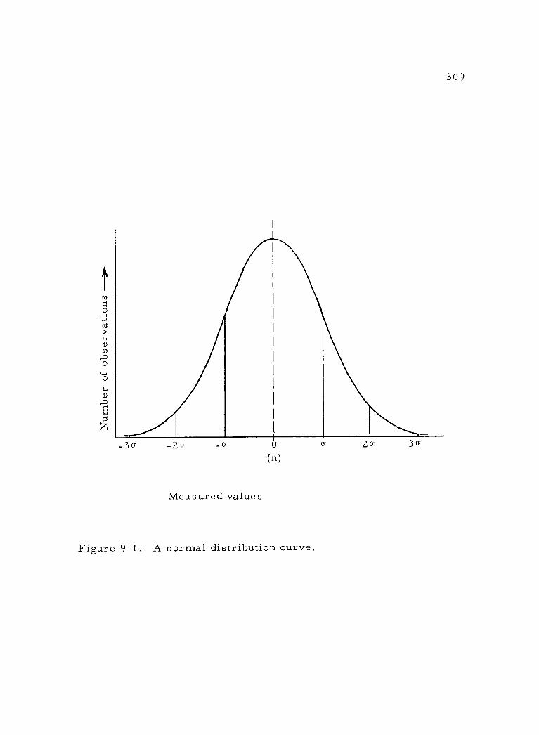
Num
ber
of ob
serv
atio
ns 4
-30- -20- _o-
Measured values
(ñ)
Figure 9 -1. A normal distribution curve.
o- 20- 3 6
309
310
are involved. The accuracy of any individual measurement (n) is
gauged by the magnitude of it deviation (A) from this mean value, or
(Equation 9 -1) A= n - ñ
On the plot in Figure 9 -1 the vertical dashed line through the apex
of the curve represents the ñ value and is arbitrarily labeled zero.
It will be noted that the distribution of positive and negative
deviations from the mean value of any given magnitude are of equal
occurrence, and that the occurrence of small deviations is more prob-
able than that of large ones. The probability of any deviation ( "error ")
being as large or larger than a given value may be calculated. The
basic "error" unit used is the standard deviation (o). The standard
deviation can be defined as the root mean square value or, for practi-
cal purposes, o = . Only 31. 7 percent of the values on a nor-
mal curve are as large or larger than ± 16. All other error units are
expressed in terms of the standard deviation. Table 9 -1 lists the
names and values of the common measures of error probability.
Table 9 -1. Measure of error probability
Name of Error Deviation - standard deviation
(A.0-)
Probability of an error exceeding such a
deviation
Probable error 0. 6745 0. 5000 Standard error
(deviation) 1. 0000 0. 3173
90% error 1. 6449 0. 1000 95% error 1. 9600 1. 0500 Two sigma 2. 0000 0. 0455 99% error 2. 5758 0. 0100 Three sigma 3. 0000 0. 0027
/

311
The foregoing discussion has considered situations where re-
peated measurements were made on the same sample, but in radio -
tracer assay it is common to make only one or two activity deter-
minations per sample. In such cases there is no .v value from which
Cr may be calculated. However, because of the nature of the Poisson
distribution, the standard deviation (o-) of a single determination (b.)
may be taken as that is the square root of the total number of
counts collected. A related unit, the relative standard deviation (or
relative o-) is defined as %/n or 1 /j. Thus, the larger the value
of n (number of counts collected), the smaller the percent standard
deviation. To achieve a given relative standard deviation it is only
necessary to continue the assay until sufficient counts are collected.
Radiotracer measurements are normally made to a one per-
cent standard deviation. In order to achieve this value it is neces-
sary to collect 10,000 counts, since when 1 /T= 1 %, n = 10, 000.
This is irrespective of the length of time required to collect this
number of counts. From this single assay one could then state that
there is a 68. 3 percent probability that the true total count was
10, 000 ± 100 counts, or (from Table 9 -2) a 95 percent probability
that the total count was 10, 000 ± 196 counts.
312
2. Contribution of background error
The 10, 000 counts collected from the above sample represent
a combination of two factors, namely sample activity and background.
The standard deviation of this measurement is therefore actually a
combination of the errors of each separate factor. When the ratio of
gross sample counting rate to background counting rate exceeds about
5 - 10, the standard deviation of the net sample activity can be found
with fair accuracy simply by taking the square root of the total num-
ber of counts collected. However, as the ratio becomes smaller,
the background error becomes increasingly significant. It is neces-
sary under these circumstances to consider the standard deviation of
the counting rate, rather than the total counts. Since the error of a
rate equals the error of the total number of counts divided by the
counting time, the standard deviation of the net counting rate for any
sample is the square root of the sum of the squares of the individual
errors, or
2 sample cts. o-2 backgd. cts. (Equation 9 -2) net ctg. rate is + tb
where is and tb represent the assay time for the sample and back-
ground, respectively.
As an example of the effect of background error on the
-
313
standard deviation of the net sample count rate, suppose that a sam-
ple is assayed for 40 minutes and 10, 000 counts collected. The back-
ground is measured for 25 minutes and a total of 2,500 counts regis-
tered. Thus, the gross sample count rate is 250 cpm, the back-
ground is 100 cpm, and the net sample activity is found to be 150
cpm. Ignoring the contribution of background error and calculating
the standard deviation as the square root of the total sample counts,
the result could be reported as 150 ± 2. 5 cpm. Using Equation 9 -2,
and taking background error into account, the results would be as
follows:
(Equation 9 -3) 1002 50 6 net ctg. rate 40 25 - 4. 5 cpm
Thus, the more accurate reporting of the counting data would be
150 ± 4. 5 cpm. It will be readily seen that it is highly desirable to
design experiments so that the counting samples have count rates at
least 5 -10 times the background. This same effect can be attained
by using various measures to reduce the background, such as "low
background counters ".
3. Optimal distribution of counting time
In an experiment where the error in the background count
rate is significant it is important to be able to estimate how long to
+
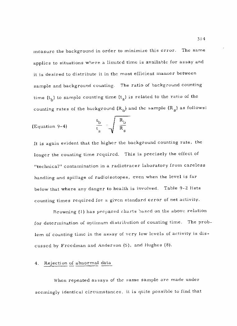
314
measure the background in order to minimize this error. The same
applies to situations where a limited time is available for assay and
it is desired to distribute it in the most efficient manner between
sample and background counting. The ratio of background counting
time (tb) to sample counting time (ts) is related to the ratio of the
counting rates of the background (Rb) and the sample (Rs) as follows:
(Equation 9 -4) tb Rb
t R s s
It is again evident that the higher the background counting rate, the
longer the counting time required. This is precisely the effect of
"technical" contamination in a radiotracer laboratory from careless
handling and spillage of radioisotopes, even when the level is far
below that where any danger to health is involved. Table 9 -2 lists
counting times required for a given standard error of net activity.
Browning (1) has prepared charts based on the above relation
for determination of optimum distribution of counting time. The prob-
lem of counting time in the assay of very low levels of activity is dis-
cussed by Freedman and Anderson (5), and Hughes (8).
4. Rejection of abnormal data
When repeated assays of the same sample are made under
seemingly identical circumstances, it is quite possible to find that
II
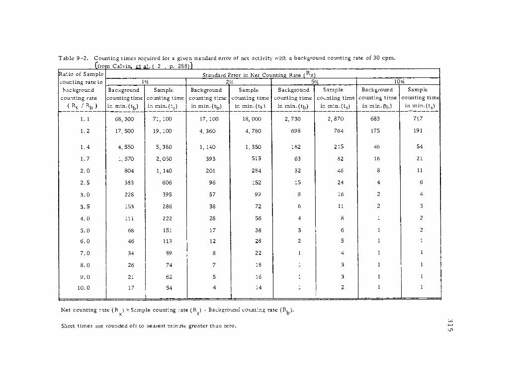
Table 9 -2. Counting times required for a given standard error of net activity with a background counting rate of 30 cpm. from Calvin al. ( 2 . p. 288
Ratio of Sample counting rate to
Standard Error in Net Counting Rate (Rx) 1% 2% 5% 10%
background Background Sample Background Sample Background Sample Background Sample counting rate counting time counting time counting time counting time counting time counting time counting time counting time
( Rs / Rb ) in min. (tb) in min. (ts) in min. (tb) in min. (ts) in min. (tb) in min. (ts) in min. (tb) in min. (ts)
1. 1 68, 300 71, 100 17, 100 18, 000 2, 730 2, 870 683 717
1. 2 17, 500 19, 100 4, 360 4, 780 698 764 175 191
1. 4 4, 550 5, 380 1, 140 1, 350 182 215 46 54
1. 7 1, 570 2, 050 393 513 63 82 16 21
2.0 804 1, 140 201 284 32 46 8 11
2.5 383 606 96 152 15 24 4 6
3.0 228 395 57 99 9 16 2 4
3.5 153 286 38 72 6 11 2 3
4.0 111 222 28 56 4 8 1 2
5.0 68 151 17 38 3 6 1 2
6.0 46 113 12 28 2 5 1 1
7.0 34 89 8 22 1 4 1 1
8. 0 26 74 7 18 1 3 1 1
9.0 21 62 5 16 1 3 1 1
10.0 17 54 4 14 1 2 1 1
Net counting rate (Rx) -Samp e counting rate (Rs) - Background counting rate (Rb).
Short times are rounded off to nearest minute greater than zero.
. et
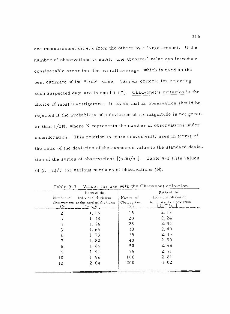
316
one measurement differs from the others by a large amount. If the
number of observations is small, one abnormal value can introduce
considerable error into the overall average, which is used as the
best estimate of the "true" value. Various criteria for rejecting
such suspected data are in use ( 9, 1 7 ). Chauvenet's criterion is the
choice of most investigators. It states that an observation should be
rejected if the probability of a deviation of its magnitude is not great-
er than 1 /2N, where N represents the number of observations under
consideration. This relation is more conveniently used in terms of
the ratio of the deviation of the suspected value to the standard devia-
tion of the series of observations [(n -rte) /T ] , Table 9 -3 lists values
of (n - ñ) /o- for various numbers of observations (N).
Table 9 -3. Values for use with the Chauvenet criterion. Rio of the -1 Ratio of the
Number of Individual deviation Numt.e: of Individual deviation
Observations to the standard devi ation Observations to -.:t-.:, stz *.dard deviation
2 1,15 15 2,13 3 1.38 20 2.24 4 1.54 25 2.35 5 1.65 30 2.40 6 1.73 35 2.45 7 1.80 40 2.50 8 1.86 50 2.58 9 1.91 75 2.71
10 1.96 100 2.81 12 2.04 200 3.02
_Z1 1. j - 57)._,:_i_ f - -_AIL _----- LL- =U -1-
317
If the calculated value of (n -ñ) / for a suspected observation exceeds
that given in Table 9 -3 for the appropriate number of observations,
the value is discarded.
For the sake of simplicity, some investigators reject sus-
pected values which deviate from the mean of a series by more than
20 or 3cr. The probabilities of such deviations are 4.5 percent and
O. 27 percent, respectively.
B. Correction Factors in Radiotracer Assay
In typical radiotracer assay the observed counting rate is not
equal to the true disintegration rate of the sample. A number of fac-
tors affect this relation between absolute disintegration rate and the
observed counting rate. Some tend to increase the observed counting
rate, while most tend to decrease it in relation to the disintegration
rate. Of these factors, some are inherent in the detectors, others
arise from the nature of the counting sample, and still others are re-
lated to the sample -to- detector arrangement. Figure 9. -2 illustrates
these factors in relation to an end -window G -M detector. The factors
to be described are largely of importance in relative beta measure-
ments, but some apply equally to gamma assay. Even though only re-
lative measurements are being made, it is necessary to understand
the effect of these factors and the corrections to be made for them.
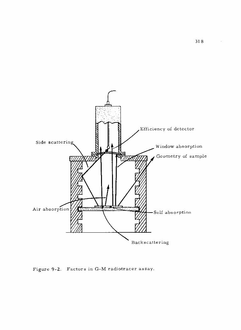
Side scatterin
Efficiency of detector
Air absorption
31 8
Window absorption
Geometry of sample
Self absorption
Backscattering
Figure 9 -2. Factors in G -M radiotracer assay.
319
1. Background
The background count rate registered on a radiation counter
can come from such varied sources as cosmic radiation, natural
radioactivity in the vicinity, artificial radioactivity (fallout), nearby
x -ray generators, and thermal or other circuit noise. Several
means are employed to reduce the background counting rate for vari-
ous counter assemblies. Detector shielding with lead or iron is
most widely utilized. In addition, coincidence circuitry and photo -
multiplier cooling in liquid scintillation counters, and anti- coinci-
dence circuitry in special low background G -M counters are excep-
tionally effective in reducing background, in some case to the level
of ten counts per hour (38). Regardless of such background reduc-
tion, the gross sample count rate (ms) always includes some back-
ground count rate (mb). The net observed counting rate (mo) due to
sample activity alone is, thus,
(Equation 9 -5) mo =ms - mb
By ignoring some minor factors the net observed counting
rate can now be related to the absolute disintegration rate (D) of a
sample as follows:
(Equation 9 -6) mo = DE fTfb fw fs
320
where E represents the correction for geometry and detector effi-
ciency, fT stands for the coincidence loss factor, fb is the back-
scatter factor, fw represents the factor for window and air absorp-
tion, and fs stands for the self- absorption factor. In gamma ray
measurements the latter three factors may usually be ignored.
2. Geometry
Since sample radiation is emitted equally in all directions,
the placement of the detector with respect to the sample is clearly a
primary limiting factor on the percentage of disintegrations that will
be detected. If 0 represents the solid angle subtended by the sensi-
tive volume of the detector, then 0/4rr equals the fraction of the
disintegrations that would be directed toward that sensitive volume.
Figure 9 -3 indicates this relationship and defines the values of d,
r and a.. The value of S2 /4rr for an ideal point source may be calcu-
lated as follows:
(Equation 9-7) 4n =
2 (1-cos a)=2 (1 d
-1'd2 +r2 )
In practice a counting sample is spread over an often considerable
area and is an extended source, rather than a point source.
Since it is extremely difficult to accurately calculate the solid
angle for extended sources, for comparative measurements it is
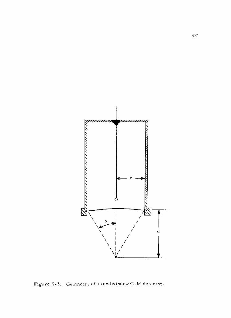
321
\ d
\ I / \ / \ / \ I
Figure 9 -3. Geometry of an end -window G -M detector.
322
strongly recommended that counting samples be prepared of uniform
size and distribution, and that they be placed at a reproducibly identi-
cal distance from the detector. A sample holding rack with several
shelves usually provides for this latter feature. Where desired, the
relative values of 4i2-
(shelf ratios) for the various shelf positions of
a sample holder can be determined as indicated in Experiment I,
Section B -5.
The value of Q for G -M and proportional end - window detectors
is always less than art, and frequently less than 11r (26). For G -M
and proportional windowless detectors, where the sample is intro-
duced into the detector, the solid angle approximates 2ir. In liquid
scintillation detectors and electrometer ion chambers a value of 47r
is attainable. An arrangement in which two windowless G -M detec-
tors are placed face to face and the sample suspended in the center
(a "4n counter ") is widely used to standardize beta sources. A com-
mon method to greatly increase the geometrical efficiency of NaI
(Tl) crystal scintillation detectors is to employ "well" crystals,
where the counting sample (usually liquid in a vial) can be inserted
deep into the crystal. In this case sample volume is limited, since
geometrical efficiency decreases sharply as the sample volume
reaches and exceeds the well capacity (21).
323
3. Detector efficiency
The factor E in Equation 9 -6 is made up of the geometry
factor c /41r and the intrinsic efficiency factor (fe) of the given detec-
tor for the radiation from a specific nuclide. Factor fe represents
the fraction of the radiation reaching the sensitive volume of a detec-
tor that is actually detected. For G -M detectors the values of fe
are 100 percent, about 96 percent, and 1 percent for alpha, beta, and
gamma radiation, respectively. With a NaI(T1) crystal scintillation
detector the gamma detection efficiency varies from 10 -60 percent
depending on the photon energy. Alpha and beta particles would not
normally penetrate to the sensitive crystal, but even so would be very
poorly detected. In an electrometer ion chamber, alpha and low
energy beta particles (C1 4, 535) would be nearly 1 00 percent detected.
Detection efficiencies would decrease with increasing beta energy,
and gamma rays would pass through virtually undetected. The value
of fe in liquid scintillation detectors is strongly dependent on beta
particle energy and degree of quenching (see Chapter 6).
Not only do detectors show a different intrinsic efficiency for
different nuclides, but the sensitivity of a specific detector to a given
nuclide will vary over a period of time. This problem particularly
plagues scintillation and proportional counters in which the detection
324
efficiency is a function of detector potential. Even slight fluctuations
in this potential can offset detection efficiency noticeably. Stability
of the high voltage supply for these counters is essential for this
reason. In addition, G -M detectors may show a variation in radial
response within the sensitive volume of the tube (20).
In organically - quenched G -M detectors failure of the quench-
ing mechanism may occur with increasing age, resulting in multiple
pulses for a single ionizing event. The factor fm (for multiple-
pulsing) must then be incorporated into factor E.
In order to determine the absolute value of E it would be
necessary to calibrate the detector with a standard source of the
same nuclide to be later assayed, making the measurements under
physical conditions identical to those later to be used (28). In most
radiotracer assays, however, only relative values of E must be
known for the purpose of correcting counting rates for variation in
efficiency with time. This is readily accomplished by making routine
measurements of the activity of a long -lived source, such as Ra -DEF
or U308. Any variation in the counting rate of this source over a
few days or weeks can be attributed to a change in detector efficiency
and all sample counts correspondingly corrected.
325
4. Coincidence loss
A radiation counting assembly requires a finite time to detect
and register each radiation particle. During this period other inci-
dent radiation is not detected. The result of this failure to resolve
two incident radiation particles that are closely spaced in time is
coincidence loss. It should be noted that disintegrations are not
evenly spaced in time. The minimum time interval between which
two events can be registered is termed the resolving time of the
counter.
Coincidence loss has several sources in a counting assembly.
Loss can occur due to the amplifier circuitry. Normally this is
negligible, since the better quality amplifiers have resolving times
of 1 -5s sec. However, in the economical "training" scalers, this
may be as high as 25Oµ sec. A more common source of coincidence
loss is the mechanical register used to record counting events.
These registers must be used with scaling circuits to minimize this
source of loss. Even then it is desirable to use a high scaling factor
(1 00, 128, 256, 1 000), if fast counting is anticipated. Davidon (27)
has prepared a nomogram for computing such register losses. In
recent years it has become common to eliminate a mechanical regis-
ter altogether and to substitute a series of scaling units employing
326
cold cathode decade tubes. To accommodate the very high counting
rates attainable with scintillation and proportional detectors it is
necessary to employ an initial "hard value" scaling unit, which is
obtainable with a 1-5p. sec. resolving time.
For the G -M counter the most important source of coinci-
dence loss is the detector. The resolving time (T) of G -M detectors
is typically 100 - 2O0µ sec. , but may be as high as 1 , O00µ sec. This
resolving time has two components: dead time and recovery time.
As seen in Figure 9 -4, for a brief interval following each ionizing
event a G -M detector is insensitive or "dead ". For a longer period
of time, during which the tube is "recovering ", it will respone to in-
cident radiation with pulses of increasing size, up to its maximum.
The total resolving time of the detector will be the dead time (Td)plus
a portion of the recovery time (T ). The portion of the recovery time r
included will be dependent on the sensitivity setting of the associated
scaler. Typically, the coincidence loss in a G -M detector begins to
be significant over about 3, 000 cpm. Scintillation and proportional
detectors, on the contrary, have such extremely short resolving
times (see Table 6 -1) that they are not the cause of significant coinci-
dence loss except at counting rates of several hundred thousand
cpm.
If the resolving time (T) of a counting assembly is known, the
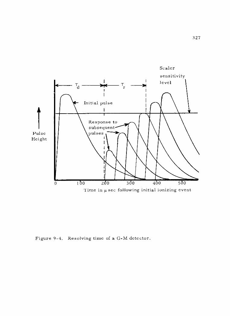
Pulse Height
Tr
Scaler sensitivity level
327
Initial pulse
Response to subsequent pulses --310.
I
100 210 310 410 5.0 Time in µ sec following initial ionizing event
Figure 9 -4. Resolving time of a G -M detector.
I
I I
I I
i
I '
I
I
I
I
I
I
I
I
328
correction for coincidence loss can be calculated. When T is in
seconds, then a counting interval of T seconds is lost for each count
registered. If m represents the observed counting rate per second,
the lost counting time is mT second for each second of counting time,
and the net counting time per second is 1 -mT seconds. Letting n
represent the corrected counting rate per second, its value is found
as
(Equation 9 -8) m 1 -mT ' °T n 1 -mT
As an example of the use of this equation for coincidence loss
corrections, consider a situation where a counting rate of 6, 000 cpm
(i. e. , 1 00 cps) was measured with a G -M counter whose resolving
time was 200p, sec. The corrected counting rate would be calculated
as follows:
(Equation 9-9) n = 1 00 cps
1 - 1 00 x O. 0002 sec. = 1 02 cps, or 6,1 20 cpm.
By contrast where the same counting assembly observed a counting
rate of 60, 000 cpm, the corrected count rate would be:
1,000 cps (Equation 9-10) n =
1 -1,000x0.0002 sec. -1, 250 cps, or 75,000 cpm.
The percent coincidence losses in these two examples were two per-
cent and 25 percent respectively.
n 1 m =
329
The resolving time of G -M detectors can be determined by
several methods. An oscilloscope may be used to directly visualize
the resolving time, essentially as in Figure 9 -4. Another method in-
volves making a consecutive series of measurements on a nuclide of
short half -life, whose initial activity is such that considerable coin-
cidence loss occurs in the detector. As decay occurs and the count
rate decreases, correspondingly less coincidence loss occurs. The
actual extent of loss can be determined graphically and the resolving
time calculated from this (see Experiment V).
The simplest means of determining detector resolving time
is the "paired- source" method used in Experiment I, Section B -4.
This involves comparing the sum of the measured activities of two
individual sources (of approximately 7, 000 - 1 0, 000 cpm each) with
the activity of the two sources measured together. Clearly, the lat-
ter figure will be smaller because the relative coincidence loss is
greater. Let nl , n2, and n 1,
represent the true counting rates of
source 1, source 2, and both sources together, respectively, includ-
ing background, and let ml , m2, and m 1,2 equal the corresponding
observed counting rates. mb will equal the background. Then
(Equation 9 -1 1 ) n1 +n2 =nl 2+nb
Substituting values of n from Equation 9 -8 would yield
1 , 2
330
ml m2 m 1,2 mb (Equation 9-12) 1
1 - m2T 1 - m1,2T 1 - mbT
This leads to a quadratic equation for T. Normally a simplified
approximation is used as follows:
(Equation 9-13) T -
5. Backscattering
m1 + m2 - m1,2 - mb
2 2 2
m1,2 - ml - m2
Radiation from a sample which is emitted in a direction away
from the detector into the backing material and is subsequently scat-
tered back toward the detector is said to be "backscattered ". The
effect is to increase the apparent counting rate of the sample. Back -
scatter is primarily a phenomenon of 21r beta assay (25).
The backscatter factor (fb) can be determined experimen-
tally by first assaying a sample mounted on mylar film, and subse-
quently measuring the count rate with various thicknesses of backing
material beneath it. It will be found that the observed counting rate
increases directly with increased thickness of backing up to a "satura-
tion" value (39). Theoretically this saturation thickness would be at
0. 5 of the beta particle range, but in practice it occurs at about 0. 2
of the range value. This density thickness is called the saturation
backscattering thickness for that radiation.
- m T 1
+ +
331
As will be seen in Figure 9 -5, backscatter increases more
rapidly with increasing backing thickness (d), the lower the beta
energy and the higher the atomic number of the backing material.
However, the ultimate fb value attained (at saturation backscatter-
ing thickness) is independent of beta energy within a range for a
given backing material. In addition, the value of the saturation back-
scattering thickness (in mg /cm2) for a given beta energy is approxi-
mately the same for all backing materials.
The value of fb at saturation backscattering thickness is
directly related to the atomic number of the backing material as
shown by Figure 9 -6. This relationship can be used to advantage to
increase the counting rate of weak samples. To this end it will be
noted that lead and platinum sample planchets would give fb values
of about 1. 80, compared to the value of about 1.30 for the commonly
used aluminum planchets.
In practice, because of the variation of fb with backing
thickness up to the saturation value, it is necessary to use sample
planchets of saturation backscattering thickness for the radiation
being assayed. It is further advisable to employ planchets of the
same material throughout a given series of experiments where com-
parisons will be made. Furthermore, a planchet designed to give
saturation backscattering thickness for C14 assay (point 1 on

2.0-
;, o ú1.50- (d
4.1
s-i
a)
cd . 25 -
m
cd
1 . 00 /
1
-+-
C14 /// / P32
14
332
Saturation Backscatter
P32
Saturation Backscatter
Backing Thickness (d) ---_
Figure 9 -5. The effect of beta energy and backing thickness on backscatter.
U
---
i C
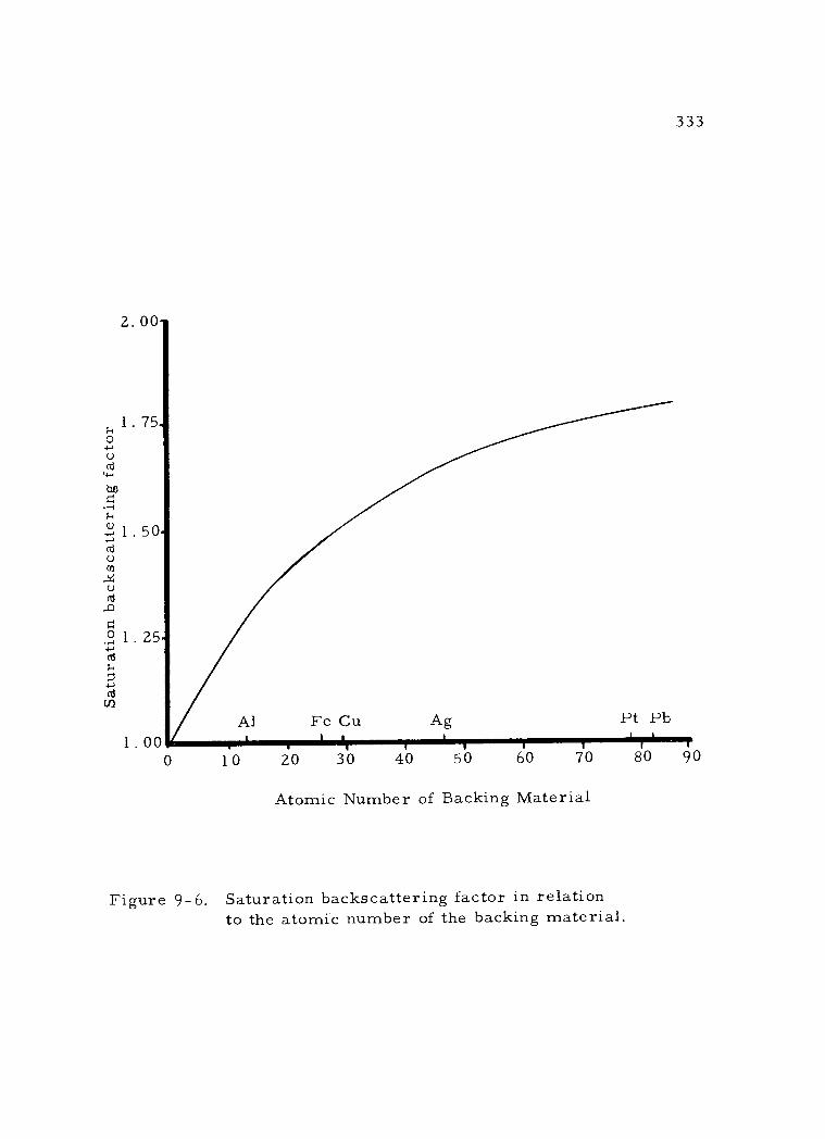
2. 00
1.00 0
Al Fe Cu Ag Pt Pb
10 20 30 40 50 60 70
Atomic Number of Backing Material
Figure 9 -6. Saturation backscattering factor in relation to the atomic number of the backing material.
80
333
90
1. 75
oa C
° 1. 50 m
7 b y
334
Figure 9 -5), could be too thin for P32 assay (point 2 on Figure 9 -5),
because only slight variation in thickness from planchet to planchet
would produce a significant difference in counting rate observed.
Thus, planchets must be selected with a view to the nuclides to be
assayed in them.
A certain amount of side scattering of radiation into the de-
tector may occur (see Figure 9 -2). In beta assay this can increase
the observed counting rate noticeably if material of high atomic num-
ber is near the source or detector. For this reason sample holders
are usually of lucite or other low Z material.
6. Absorption
An often considerable fraction of the radiation emitted in the
direction of a detector may be absorbed before it reaches the sensi-
tive volume of the detector. This absorption may occur in the sam-
ple itself (self -absorption), in the intervening air space, or in the
window of the detector (G -M and proportional type). The latter two
areas of absorption are included in the correction factor fw, while
self- absorption, the more important consideration, is designated f .
s
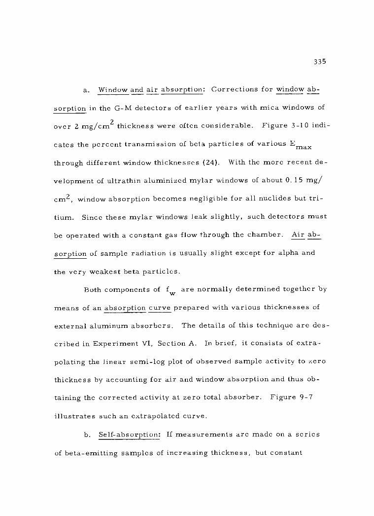
335
a. Window and air absorption: Corrections for window ab-
sorption in the G -M detectors of earlier years with mica windows of
over 2 mg /cm2 thickness were often considerable. Figure 3 -10 indi-
cates the percent transmission of beta particles of various Emax
through different window thicknesses (24). With the more recent de-
velopment of ultrathin aluminized mylar windows of about 0.15 mg/
cm2, window absorption becomes negligible for all nuclides but tri-
tium. Since these mylar windows leak slightly, such detectors must
be operated with a constant gas flow through the chamber. Air ab-
sorption of sample radiation is usually slight except for alpha and
the very weakest beta particles.
Both components of f are normally determined together by
means of an absorption curve prepared with various thicknesses of
external aluminum absorbers. The details of this technique are des-
cribed in Experiment VI, Section A. In brief, it consists of extra-
polating the linear semi -log plot of observed sample activity to zero
thickness by accounting for air and window absorption and thus ob-
taining the corrected activity at zero total absorber. Figure 9 -7
illustrates such an extrapolated curve.
b. Self- absorption: If measurements are made on a series
of beta - emitting samples of increasing thickness, but constant
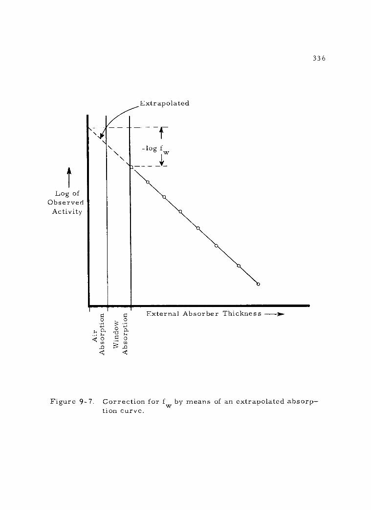
Absorption
Log of Observed Activity
Extrapolated
- --I -log f w
External Absorber Thickness -
336
Figure 9 -7. Correction for f by means of an extrapolated absorp- w
tion curve.
\
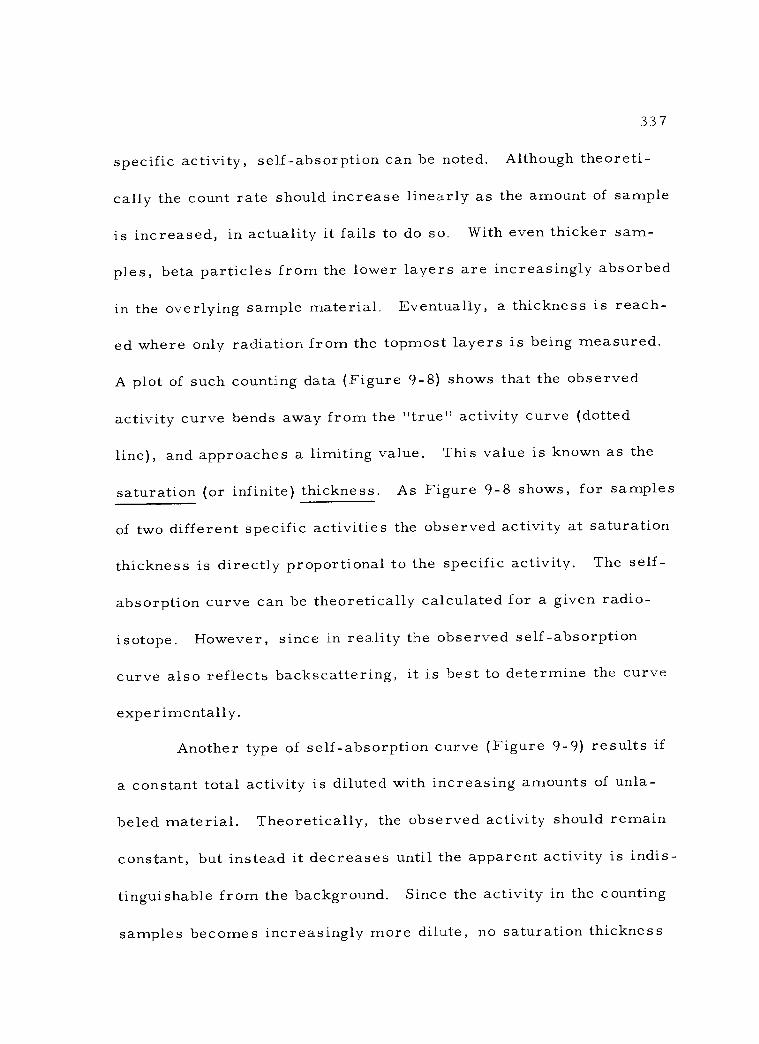
337
specific activity, self- absorption can be noted. Although theoreti-
cally the count rate should increase linearly as the amount of sample
is increased, in actuality it fails to do so. With even thicker sam-
ples, beta particles from the lower layers are increasingly absorbed
in the overlying sample material. Eventually, a thickness is reach-
ed where only radiation from the topmost layers is being measured.
A plot of such counting data (Figure 9 -8) shows that the observed
activity curve bends away from the "true" activity curve (dotted
line), and approaches a limiting value. This value is known as the
saturation (or infinite) thickness. As Figure 9 -8 shows, for samples
of two different specific activities the observed activity at saturation
thickness is directly proportional to the specific activity. The self -
absorption curve can be theoretically calculated for a given radio-
isotope. However, since in reality the observed self- absorption
curve also reflects backscattering, it is best to determine the curve
experimentally.
Another type of self- absorption curve (Figure 9 -9) results if
a constant total activity is diluted with increasing amounts of unla-
beled material. Theoretically, the observed activity should remain
constant, but instead it decreases until the apparent activity is indis-
tinguishable from the background. Since the activity in the counting
samples becomes increasingly more dilute, no saturation thickness
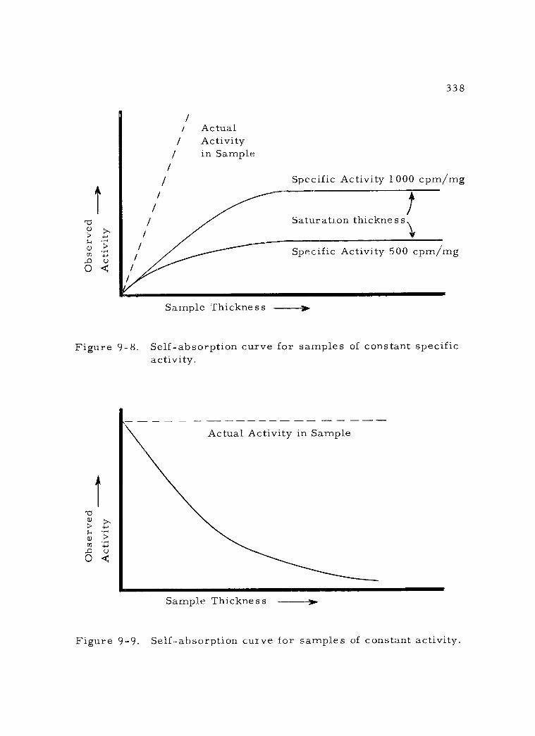
Observed
/ Actual / Activity
in Sample
338
Specific Activity 1000 cpm /mg
Saturation thickness '!I
Specific Activity 500 cpm /mg
Sample Thickness --- Figure 9 -8. Self- absorption curve for samples of constant specific
activity.
Actual Activity in Sample
Sample Thickness
Figure 9 -9. Self -absorption curve for samples of constant activity.
/ /
/
/ /
/ /
fr
-lop 4
b
o
339
is reached"
Self-absorption eorrection is prirnarily a problern in the assay
of low energy beta-ernitters, su.ch a" H3, CL4, S35 and C^45 123,
29, 32*37, 41*4Z-1" High energy beta-ernitters suffer relatively little
self -absorption with the usual sarnple thicknesses (less than f'S rng/
crnz). Alpha ernitters, because of their typically short range, are
aknost always rneasured at saturation thickness, whereas galnrrra
radiation is readily transrnitted through the thickest assay sarnple
with virtually no absorption. The effect of self-absorption is rnore
pronounced when iiquid sarnples of beta-ernitters are assayed and,
in fact, is a lirniting factor on the volurne of liquid that can be accorn-
rnodated. Self-absorption rnight be considered as an analogous effect
to quenching in liquid scintillation detection, the correction for which
has been discussed in Chapter 6"
Several rnethods have been used to correct for the effect of
self-absorption on counting rate. Sorne workers resort to preparing
all sarnples to a constant thickness" .W'hile accurate for cornparative
purposes, this is an extrernely tedious technique" For rough rneas-
urernents, direct plating frorn solution rnay be used to produce sarn-
ples of negligible thickness, so that seLf -absorption is nearly elirni-
nated. This requires preparing sarnples of less than I rng/crn?
thickness for Cl4 arrd S35, which are quite difficul-t to secure with a
340
uniform surface, because of uneven drying. By contrast, if suffi-
cient sample material is available, all samples can be prepared at
saturation thickness. In this case the observed count rate will be
directly proportional to the specific activity of the sample, not to its
thickness. This method is quite satisfactory for comparative meas-
urements, although all samples so compared must be of the same
molecular composition, or else corrections for the differences will
be required.
The most generally satisfactory method for self -absorption
correction is a graphic one. It is this method that will be followed
in Experiment VI, Section C. Briefly this involves preparation and
assay of a series of samples of constant specific activity, but vary-
ing thickness. A curve is prepared of the apparent specific activity
of the samples plotted against the sample thickness in mg /cm2.
This curve is extrapolated to zero sample thickness and the specific
activity at that point regarded as the "true" specific activity of the
samples. A second curve is then prepared of percent specific acti-
vity (apparent specific activity/ "true" specific activity, i. e. , per-
centage transmission) vs. sample thickness. Correction values can
then be found from this curve for transmission at any sample thick-
ness up to saturation thickness. Figure 9 -10 shows a schematic ver-
sion of such a curve. In Experiment VI directions are given for
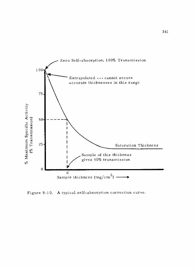
341
1 00
75
Zero Self- absorption; 100% Transmission
Extrapolated - -- cannot secure accurate thicknesses in this range
Saturation Thickness
Sample of this thickness gives 50% transmission
d Sample thickness (mg /cm2) -i
Figure 9 -10. A typical self -absorption correction curve.
ê
áE m
H ~
ro E i s'-'
5
25
0
1
1
1
I.
I
342
preparing a correction curve for BaC14O3 samples. A correction
curve thus prepared is strictly applicable only to the radiation count-.
er and molecular form of sample used in its formulation.
C. Summary
In making comparative measurements of beta sample activi-
ties with G -M counters corrections for all the factors in Equation
9 -6, except fT and fs, and background can be avoided by keeping
assay conditions constant. If sample count rates are held below
about 3, 000 cpm, fT may be ignored. Correction for self- absorp-
tion is made by means of a correction curve (Figure 9 -10). By con-
trast, when the activities of different samples of the same gamma -
emitting nuclide are being compared, all the correction factors may
be kept constant, unless an exceedingly high count rate introduces
some coincidence loss. It must be stressed that such comparisons
are possible only when assays have been carried out under conditions
as nearly identical as possible. For absolute activity determinations
each correction factor must be individually evaluated as outlined
above. Zumwalt (43) has thoroughly described such absolute beta
counting using an end - window G -M detector.
343
BIBLIOGRAPHY
Statistical considerations
1. Browning, W. E. , Jr. Charts for determining optimum distribu- tion of counting times. Nucleonics 9(3):63 -67. 1 951.
2. Calvin, Melvin, et al. Isotopic carbon. Techniques in its meas- urement and chemical manipulation. New York, John Wiley, 1949. 376 p.
3. Counting techniques. pt. I. Picker Scintillator (issued by Picker X -Ray Corp. ) 1 (4):1 -1 O. Dec. 2, 1 957.
4. Elmore, W. C. Statistics of counting. Nucleonics 6(1):26-34. 1 950.
5. Freedman, Arthur J. and Ernest C. Anderson. Low -level count- ing techniques. Nucleonics 10(8) 57 -59. 1 952.
6. Greenfield, M. A. and R. L. Koontz. A universal function for computing counting performance. The International Journal of Applied Radiation and Isotopes 8:205 -210. 1960.
7. Herberg, R. J. Counting statistics for liquid scintillation count- ing. Analytical Chemistry 33:1308 -1311. 1961.
8. Hughes, H. A. Reduction of counting time in low activity assays. British Journal of Applied Physics 7:41 5 -41 6. 1 956.
9. Is my nuclear instrumentation putting out valid data? Picker Scintillator (issued by Picker X -Ray Corp. ) 4(4):1 -4. May 20, 1960.
10. Jaffey, Arthur H. Statistical tests for counting. Nucleonics 1 8(1 1 ):1 80 -1 84. 1 960.
11. Jarrett, Alan A. Statistical methods used in the measurement of radioactivity. Some useful graphs. 1 946. 63 p. (U. S.
Atomic Energy Commission. AECU -262)
1 2. Kuyper, Adrian C. The statistics of radioactivity measurement. Journal of Chemical Education 36:1 32. 1959.
344
1 3. Miller, D. G. and M. B. Leboeuf. Effect of high beta backgrounds on precision alpha counting. Nucleor..ic a 11 (4):28 -31 . 1953.
14. Rainwater, L. J. and C. W. Wu. Applications of probability theory to nuclear particle detection. Nucleonics 1(2):60-69. 1 947.
15. Schuler, Robert H. Short -lived radioactivity; correction for long counting periods. Nucleonics 1 0(1 1 ):96 -97. 1 952.
1 6. Tittle, C. W. How to apply statistics to nuclear measurements. Des Plaines, Ill. , 1962. 4 p. (Nuclear- Chicago Technical Bulletin No. 14).
1 7. When do you consider a nuclear measurement to be invalid? Picker Scintillator (issued by Picker X -Ray Corp. ) 5(2)1 -2. Feb. 24)1 961 .
18. Wilson, E. Bright, Jr. An introduction to scientific research. New York, McGraw -Hill, 1952. 375 p.
19. You can't beat statistics. Picker Scintillator (issued by Picker X -Ray Corp. ) 4(2):1 -8. Dec. 29, 1 959.
Correction factors in radiotracer assay
20. Amith, Avraham and W. Wayne Meinke. Radial response of typical end - window G -M tubes. Nucleonics 1 1(5):60-61. 1 953.
21 . Baskin, R. , H. L. Demorest and S. Sandhaus. Gamma counting efficiency of two well -type NaI crystals. Nucleonics 12(8):46- 48. 1 954.
22. Bayhurst, B. P. and R. J. Prestwood. A method for estimating beta- counting efficiencies. Nucleonics 17(3):82 -85. 1959.
23. Beltz, Richard E. Self- absorption correction in the use of tri- tium- labeled substrates for enzyme assays. Analytical Biochemistry 2:303 -31 6. 1 961 .
24. Chang, Chia -Hua and C. Sharp Cook. Relative transmission of beta particles through G -M counter windows. Nucleonics 1 0 (4):24 -27. 1952.

345
25. Christian, Darleane, Wayne W. Dunning and Don S. Martin, Jr. Backscattering of beta rays in windowless G -M counters. Nucleonics 1 0(5):41 -43. 1 952.
26. Cook, G. B. , J. F. Duncan and M. A. Hewitt. Geometrical efficiency of end - window G -M counters. Nucleonics 8(1):24- 27. 1951.
27. Davidon, William C. Nomogram for computing register losses. Nucleonics 10(1 2):76 -77. 1 952.
28. Gleason, G. I. , J. D. Taylor and D. L. Tabern. Absolute beta counting at defined geometries. Nucleonics 8(5):1 2-21. 1951.
29. Graf, Walter L. , C. L. Comar and Ira B. Whitney. Relative sensitivities of windowless and end - window counters. Nucle- onics 9(4):22 -27. 1951.
30. Libby, W. F. Measurement of radioactive tracers. Analytical Chemistry 1 9:2-6. 1947.
31. Loevinger, Robert and Mones Berman. Efficiency criteria in radioactivity counting. Nucleonics 9(1 ):26 -39. 1 951
32. Muramatsu, Masami and Harris Busch. Self- absorption correc- tions for C14- labeled protein. Analytical Biochemistry 4:384- 394. 1 962.
33. Nervik, W. E. and P. C. Stevenson. Self- scattering and self - absorption of betas by moderately thick samples. Nucleonics 1 0(3):1 8-22. 1952.
34. Poddar, R. K. Quantitative measurement of S35 samples. Nucleonics 1 5(1 ):82 -83. 1 957.
in biological
35. Pawsner, E. R. Self- absorption of carbon -14 samples on thin paper planchets. The International Journal of Applied Radia- tion and Isotopes 1 0:22 -29. 1 961.
36. Reid, Allen F. , Adele S. Weil and J. R. Dunning. Properties and measurement of carbon 14. Analytical Chemistry 1 9:824- 827. 1 947.
346
37. Schweitzer, George K. and Bernard R. Stein. Measuring solid samples of low- energy beta emitters. Nucleonics 7(3):65 -72. 1 950.
38. Softky, S. D. and R. E. Nather. Low -background counter for solid ß- emitting samples. Nucleonics 1 5(5):90-93. 1957.
39. Tittle, C. W. How to compute absorption and backscattering of beta rays. Des Plaines, Ill. , 1961. 4 p. (Nuclear- Chicago Technical Bulletin No. 8).
40. Upson, U. L. Beta energy dependence in end - window G -M tubes. Nucleonics 11 (1 2):49 -54. 1 953.
41. Wick, Arne N. , Harry N. Barnet and Nancy Ackerman. Self - absorption curves of C14- labeled barium carbonate, glucose, and fatty acids. Analytical Chemistry 21 :1 51 1 -1 51 3. 1 949.
42. Yankwich, Peter E. , Thomas H. Norris and John Huston. Cor- recting for the absorption of weak beta -particles in thick sam- ples. Analytical Chemistry 19:439 -441. 1947.
43. Zumwalt, Lloyd R. Absolute beta counting using end - window Geiger -Mueller counters and experimental data on beta - particle scattering effects. 1950. 76 p. (U. S. Atomic Energy Commission. AECU -567).
347
CHAPTER 10 - DESIGN AND EXECUTION OF RADIOTRACER EXPERIMENTS
It would be most difficult to determine the magnitude of the
contribution radioactive tracer methodology has made to biological
investigations. The use of radioactive isotopes allows the tracing of
tagged molecules through biological systems in a manner hitherto
impossible. It is for this reason that radiotracers have been employed
so extensively in biochemical studies of intermediary metabolism and
in physiological studies in general. However, radiotracer method-
ology has certain inherent limitations and problems that must be un-
derstood and evaluated if it is to be used successfully. The bearing of
these limitations on the proper design and execution of radiotracer ex-
periments will be examined in this chapter.
A. Unique Advantages of Radiotracer Experiments
The degree of magnification possible using radiotracers far
exceeds that with most other chemical or physical methods. For ex-
ample, a cubic centimeter of carrier -free tritium gas (specific acti-
vity 2. 59 curies /cc) can be diluted by a factor of 1012 to yield a speci-
fic activity of only 2. 59 x 10 -6 µc /cc and yet the resultant activity is
readily detectable. Such a degree of magnification is comparatively
several degrees of magnitude greater than the optical magnification
348
obtainable with the electron microscope. It is thus possible to detect
the occurrence of metabolic substances which are normally present in
tissues at such low concentrations as to defy the most sensitive chemi-
cal methods of identification. An example would be the tracing of tri-
tiated thymidine incorporation into nucleic acids in cell nuclei.
Perhaps the most outstanding advantage of the use of radioiso-
topes in biology is the opportunity afforded to trace dynamic mecha-
nisms in organisms. Such biological phenomena as ion transport
across cell membranes, steady state dynamics, intermediary meta-
bolism, or translocation in plants could only be approached indirectly
before the advent of radiotracer methods. Unfortunately, the very
fact that radiotracer studies so commonly involve such dynamic con-
ditions frequently renders the interpretation of experimental results
most difficult.
The use of the isotope effect to study rate -determining steps
in a sequence of biochemical reactions represents an additional, al-
though lesser, advantage of radiotracer methodology. The term iso-
tope effect refers to the influence upon reactions due to the presence
of a radioisotope label. This effect, thus, can be used to advantage
in a limited number of cases to determine the kinetics of certain bio-
chemical reactions.
Despite such advantages, indiscriminate use is often made of
349
radiotracers in biological investigations. It should be clearly under-
stood that radiotracers are not magic tools whose use guarantees suc-
cess in even the most difficult experimental situations. Instead, their
use involves added complexity - -- detection equipment, safety precau-
tions, etc. Even more careful experimental design than in non -tracer
experiments is required. The problem of data analysis and the draw-
ing of reasonable conclusions therefrom is also made more difficult.
In short, radiotracers should only be resorted to when they offer a
unique method of obtaining a definitive answer. The possibility of
achieving the desired results by employing simpler conventional me-
thods should always be explored first.
B. Preliminary Considerations in Design of Radiotracer Experiments
1. Basic assumptions on which the validity of radiotracer experiments rest
Experiments with radiotracers will be valid and interpretations
of results meaningful only in so far as careful consideration has been
given to certain basic assumptions. These relate to the behavior and
nature of the radioisotope preparation introduced into the experimental
organism. It must be assumed that:
a. There is no significant isotope effect: It has been previous-
ly stated that the primary assumption in all radiotracer work is that a
350
radioactive isotope behaves chemically in a fashion identical to the
stable isotopes of the same element. This is not strictly true in all
cases. Because the respective nuclei differ (if only slightly) in mass
and, hence mobility, they can be expected to show variation in reaction
rates. Ordinarily this difference in reaction rate is not great enough
to be significant in biological tracer experiments. Since this differ-
ence is inversely related to the square root of the masses of the iso-
topes involved, it is apparent that an isotope effect will be of signifi-
cance only for elements of low atomic weight.
The isotopes of hydrogen present the extreme case. Thus,
HZ, H2(D), and H3(T) could scarcely be expected to act as the same
substances chemically, since the relative mass differences are so
great. For this reason, tritium cannot be uncritically employed as a
tracer for hydrogen in regard to reaction rates, although, of course,
this does not preclude its use to determine hydrogen location in an or-
ganism.
Eidenoff (7, p. 222 -226) has discussed the isotopic effect as it
relates to C -H and C -T bonds. The magnitude of the effect for the
isotopes of carbon is much less than for hydrogen. Rabinowitz, et al.
(6) found that urea -C' 2 was hydrolyzed by urease at a rate about ten
percent faster than urea -C14. An excellent survey of this problem of
biological fractionation of isotopic mixtures by proti.sta, higher plants,

351
mollusca and vertebrates has been made by Bowen (1).
b. There is no damage to the experimental organism: It is es-
sential that radiation from the tracer dose used does not elicite a res-
ponse from the experimental organism which would distort the experi-
mental results. The amount of activity employed should be restricted
to the minimum necessary to permit reasonable counting rates in the
samples to be assayed. The possibility of excessive concentration of
the tracer compound in certain tissues and the degree of radiosensiti-
vity of these tissues must also be carefully considered, especially
when alpha- or beta -emitting tracers are used. Fortunately the sensi-
tivity of most radioactivity assay methods minimizes the necessity of
employing tracer doses of such a magnitude that any detectable radia-
tion damage occurs. Furthermore, the possibilities of interference
due to physiological response to radiation are minimized by the fact
that most studies are short term and thus completed before any latent
radiation effects appear.
c. There is no deviation from the normal physiological state:
If, in order to administer the required tracer activity, the chemical
level of the compound given to an organism greatly exceeds the normal
physiological level, the experimental results are open to question. In
other words, the specific activity of the tracer compound must be suf-
ficiently high for the total chemical level administered to be within

352
the physiological range. As an example, C136 would be potentially
quite useful for biological investigation except for the fact that the
maximum specific activity obtainable in the inorganic form is about
100 µcg Cl. This stands in contrast to specific activities of C14 (as
BaC14O ) of up to 2. 2 curies /g of carbon. 3
d. The physical state of the compound is acceptable: Some
carrier -free tracers (usually cations) in solution behave like colloids
rather than true solutions. The term radiocolloid has been applied to
such substances. Radiocolloids behave quite differently in biological
systems than do ions of the same isotope. Stokinger (9) has examined
the problem of phagocytosis of radiocolloids in organisms and the con-
sequent effect on their tissue distribution. Thus, an ill- defined physi-
cal state of the radiotracer compound leads to difficulty in interpret-
ing its physiological and metabolic behavior.
e. The chemical form of the compound is well defined: Anoma-
lous experimental results have frequently been traceable to the chemi-
cal form of the administered radiotracer. Since reactor production of
radioisotopes often results in the formation of complex mixtures of
compounds, this is not surprising. In one case involving phosphate-
P32 2 uptake in plants, the unexpected experimental results were ex-
plained by the fact that a large percentage of the tracer dose was actu-
ally in the form of phosphite -P32.
353
The radiochemical purity of a compound cannot be assumed.
The presence of other radioactive species in low chemical concentra-
tion, but high specific activity is frequently encountered. Cohn (5)
has examined the sources, detection, and means of removal of such
radioactive contaminants. The problem of radiochemical purity with
respect to the chemical state of tritium and C14-labeled compounds
is still more acute. Because of the short range of their beta parti-
cles, the radiation dose delivered to such compounds by their own
radiation leads to self- decomposition (radiolysis). This problem is
more fully discussed by Lemmon (4) and Tolbert (7, p. 64 -68, 10).
f. Only the labeled atoms are being followed: It must never
be assumed that the appearance of the radioactive label in a given
tissue indicates the presence of the administered compound. It is the
labeled atoms that are being followed, not the intact compound. Not
only may metabolic reactions separate the label from the original
compound, but chemical exchange may occur, as well. Such chemi-
cal exchanges particularly plague many experiments with tritium -
labeled compounds. The extent of chemical exchange is strongly de-
pendent on the molecular species involved and the position of the label
in the molecule.
354
2. Evaluation of the feasibility of radiotracer experiments
a. Availability of the radiotracer: A primary consideration is
whether a radioisotope of the element to be traced is available with the
proper characteristics (half -life, particle energy, etc. ) For ex-
ample, although radioisotopes of oxygen and nitrogen would be highly
desirable in biological investigations the longest lived radionuclides
available of these elements have half -lives of two and ten minutes,
respectively. Clearly, such short half -lives render these isotopes
useless for all practical purposes. On the other hand, for several
elements a choice of usable radioisotopes may be available, such as
Na22 or Na24 and Co58 or Co60
A second consideration is whether the tagged compound de-
sired is commercially available or can even be produced. The num-
ber of labeled compounds available is large indeed, and most radio-
chemical suppliers will attempt custom syntheses of unstocked com-
pounds. However, in some cases, it is not economically feasible
or even possible to introduce a given radioactive atom into the mole-
cular structure under consideration. Furthermore, the specific acti-
vity secured may be too low for the proposed experimental use of the
tagged compound. This general problem will be considered in further
detail in the next chapter.

355
b. Feasibility of detection: The degree to which the administered
tracer dose will be diluted by the biological system must be most carefully
evaluated. Dilution must not be so great that the activity of the counting
samples will be below the limits of detection. In situations where sample
specific activity is unavoidably low, it will be necessary to select a suffi-
ciently sensitive detecting system (see Table 6 -1). Furthermore, the
anticipated sample specific activity and means of detection will often
dictate the choice of counting sample preparation. This choice will also
influenced by the number of counting samples to be prepared and the re-
quired precision of the experiment.
c. Evaluation of hazard: The first consideration is the pos-
sibility of harm to the experimenter himself or his co- workers. In
the great majority of radiotracer experiments the hazard from direct
external radiation does not pose a serious problem. The one excep-
tion is where high levels (millicuries) of gamma emitter are employ-
ed. For example, 10 millicuries of sodium -24 will deliver a dose of
about 19 milliroentgens per hour (at one meter distance). The major
item of concern in the use of alpha or beta emitting tracers is the
possibility of internal contamination. This problem is made acute
where the sample is in the form of an aerosol or a dry powder at
some stage of the experiment. A more complete discussion of radio -
tracer hazards will be found in Chapter 12.
Radiation damage to the biological system under study may oc-
cur at two levels -- the physiological and the histological. In general,
higher radiation doses are required to elicit the latter type of damage.
Whenever it is suspected that radiation damage is influencing
356
the physiological response of the organism, it is advisable to repeat
the experiment with lower levels of radioactivity, while maintaining
the same total chemical level of the administered compound. Biologi-
cal effects of radiation from radiotracer doses have been reported as
follows: 0. 045 µc I 131 /g of body weight in mice, 0.8µc P32 32 /g of
body weight in mice, 47 p Na 24/g body weight in mice and rats, 0. 5
µc Sr /g 89 body weight in mice and rats, 0. 05 µc P32 /ml 32 of rearing
solution for mosquito larvae, 2 pc P32 /liter of nutrient solution for
barley plants.
Attention must also be given to the disposal of radioactive
wastes resulting from the experiment, such as excreta, carcasses,
or large volumes of solutions. The method of disposal possible will
depend on the specific radioisotope present, its concentration and ac-
tivity, and the nature of the waste. Disposal must conform to the
Code of Federal Regulations, Title 10, Part 20. Methods and princi-
ples of waste disposal will be further discussed in Chapter 12.
d. Evaluation of proposed methodology and data analysis: Ex-
perimental data are useless until they are interpreted. This is parti-
cularly true in radiotracer experiments involving biological systems.
Attention must first be given to a clear statement of the hypothesis to
be tested. Next, the sampling process to be followed mustbe carefully
evaluated. Only then can proper methods of data analysis be selected.

357
For further discussion of this aspect of experimental design the
reader is referred to the excellent general volume by Wilson (12).
The precision required in the proposed experiment must be
clearly established. In radiotracer investigations this is heavily in-
fluenced by the method of sample preparation and the assay technique
employed. The inherent variability in organisms adds further compli-
cations where highly precise results are desired. If one is looking
for only a small experimental difference, a high degree of precision
is critical for the success of the investigation. Such a degree of pre-
cision is not always compatible with the nature of radiotracer metho-
dology. Chapter 9 considers the analysis of data in radioactivity
measurements in greater detail.
C. Basic Features of Experimental Design
1. The nature of the experiment
It should never be thought that the use of radiotracers will
allow an investigator to approach an experimental problem with a les-
ser degree of preparation and forethought than is necessary in non -
tracer experiments. Indeed, the tracer method requires that the in-
vestigator be even more intimately familiar with the specific organ-
ism to be used and the general nature of the problem. In short, there
is no substitute for a thorough knowledge of one's own field.
358
Radiotracers must always be regarded as only a tool, not a panacea.
When radioisotopes are used in a dynamic biological system,
one of the commonest difficulties is that of failure to recognize the
kinetics of the system. It is of prime importance to consider the pos-
sible pathways a labeled compound may take in the experimental or-
ganism, based on what is known about the kinetics of the system al-
ready. The effect of such factors as the existence of alternate path-
ways, the extent of dilution from endogenous sources, the possibility
of the re -entry of degraded products into the system, the degree of
chemical exchange of the labeled atoms, and the general consideration
of whether one is dealing with an open or closed system, must all be
pondered. Even if the kinetics of the system under consideration are
not well known, the investigator must still be aware of their possible
influence on his experimental results.
A recent outstanding volume by Sheppard (8) has discussed ex-
tensively what may by expected to occur in a kinetic system following
the introduction of labeled material into a portion of it. The author
uses a mathematical treatment of multicompartmental systems such
as are presented by living organisms. A considerable volume of liter-
ature concerning the experimental design necessary in radiotracer
turnover measurements studies has been written, of which the articles
by Zilversmit and Shore (13), Lax and Wrenshall (3), Kamen (7,
359
p. 21 0 -21 6), and Jeffay (7, p. 21 7 -221) might be cited.
2. The scale of operation
A basic requirement in designing a radiotracer experiment is
the calculation of the amount of labeled compound which will be needed.
In other words, will kilogram or milligram quantities be required?
The factors affecting this calculation will first be discussed and then
specific examples will be cited.
a. The labeled compound: If the tracer compound must be
synthesized, the starting amount required to give the desired yield
must be determined. On the other hand, if the tagged compound is to
be purchased, the factor of cost enters into consideration. It is fre-
quently necessary to redesign an entire experiment on the basis of
the cost factor alone. For example, if one were using hydrocorti-
sone -4 -C14 (commercial price $36 /mg), it would be somewhat un-
realistic to design a single tracer experiment requiring gram amounts.
b. The biological system: The extent to which the labeled
compound will be diluted in the experimental organism is a major con-
sideration in determining the quantity to be administered. This dilu-
tion is primarily a function of the relative size of the biological system
chosen. Clearly, a smaller quantity of tracer compound will be need-
ed for a given purpose in a rat than in a dog, or in a seedling plant
360
than in a mature tree. The use of microorganisms in radiotracer in-
vestigations offers the distinct advantage of requiring very small quan-
tities of active material. This is most beneficial where the tracer
compound used is available in quite limited amounts. When no reliable
basis exists for calculating the extent of anticipated dilution, liberal
estimates should be made to account for unexpectedly large dilution.
In addition, the number of biological specimens necessary to achieve
a given statistical validity must be determined in advance.
c. Purpose of the experiment: The purpose of the experiment
will also be a determining factor in the calculation of the scale of oper- 14
ation. In some cases, as in assaying respired C 02, the purpose
will be to merely identify a labeled compound. In other investigations
the location of a labeled compound is sought, as in the use of tritiated
thymidine to trace DNA localization in chromosomes. On the other
hand, it may be desired to identify the labeling pattern in a compound
synthesized by the organisms, as in a study of the precursor -product
relation. Such investigations require not only isolation of the labeled
compound, but further processing (degradation). An example would be
the identification of the labeling pattern in amino acids synthesized by
yeast cells exposed to C14O (Experiment A). Where the labeled pro - 2
duct is to be degraded to determine the pattern of labeling, the scale
of operation must be large enough to provide sufficient sample material
361
for the chemical operations involved (a usual minimum is 500 mg).
This may necessitate adding non -radioactive carrier material to the
sample.
3. Detection efficiency
A primary consideration as to the size of the initial tracer dose
required is the detection efficiency of the counting system to be em-
ployed. This, along with the degree of counting precision desired,
sets a minimum level on the required activity in counting samples.
Furthermore, the detection efficiency of the various counting systems
is dependent on the radioisotope being assayed. Thus, a much higher
activity of the gamma- emitter 1131 would be required if the detector
was to be a G -M tube, than if a NaI (T1) scintillation detector were
used. For discussion of the relative efficiencies of the various detec-
tion systems see Chapters 4 - 6. Other factors affecting counting ef-
ficiency, such as self absorption, coincidence loss, etc. , have been
considered in Chapter 9.
4. Specific activity
From the previous considerations, the scale of operation has
been calculated, i. e. the amount of the labeled compound that must be
put into the biological system to secure the desired sample. Now,
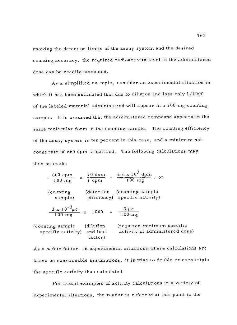
362
knowing the detection limits of the assay system and the desired
counting accuracy, the required radioactivity level in the administered
dose can be readily computed.
As a simplified example, consider an experimental situation in
which it has been estimated that due to dilution and loss only 11000
of the labeled material administered will appear in a 100 mg counting
sample. It is assumed that the administered compound appears in the
same molecular form in the counting sample. The counting efficiency
of the assay system is ten percent in this case, and a minimum net
count rate of 660 cpm is desired. The following calculations may
then be made:
660 cpm 10 dpm 6. 6 x 10³ dpm 100 mg x
1 cpm 100 mg or
(counting (detection (counting sample sample) efficiency) specific activity)
3 x 10⁻³µc 100 mg x 1000
3 µc 100 mg
(counting sample (dilution (required minimum specific specific activity) and loss activity of administered dose)
factor)
As a safety factor, in experimental situations where calculations are
based on questionable assumptions, it is wise to double or even triple
the specific activity thus calculated.
For actual examples of activity calculations in a variety of
experimental situations, the reader is referred at this point to the
,
363
selected radiotracer experiments in Part Three. In the section of
each experiment entitled "Experimental Design" the determination of
the required activity and chemical level of the respective tracer doses
has been carefully analyzed. Step -by -step calculations are indicated.
Although the examples given will by no means cover all cases, they
do illustrate the general pattern of activity calculations.
The problem of background radiation must also be considered.
Its effect on counting accuracy has been discussed previously in Chap-
ter 9. Background radiation can be particularly troublesome in auto -
radiography, where it results in a fogging of the film. This necessi-
tates having a significant amount of activity in the sample to be auto -
radiographed in order to give a good image in a reasonably short ex-
posure time.
5. Anticipated experimental findings
Certain features of experimental design relate to the antici-
pated experimental results. If a time course is to be followed, the
number of samples to be collected and the collecting intervals to give
the best kinetic information must be decided in advance. With refer-
ence to procedures involving paper chromatography, one must know
the optimal amount of sample that can be applied on the particular
chromatograph paper to be used. It is of special importance to
364
design the experiment so that the information derived can be inter-
preted meaningfully. To this end it must be decided whether count-
ing results will be expressed as percentage yield or specific acti-
vity (see section E below).
D. Execution of Radiotracer Experiments
A major portion of this volume has been concerned with as-
pects of executing radiotracer experiments (sample preparation,
assay, etc. ) However, a few specific points should be mentioned
here. An initial step is to determine the radiochemical purity of
the labeled compound. Some degree of radiolysis in compounds
labeled with H3, C14, or S35 must be assumed if they have been
stored for any length of time. Chromatographic purification before
use should be a routine procedure.
It must never be assumed that the employment of radiotracer
methodology allows a decreased concern for accuracy in the routine
procedures of weighing and measuring. On the contrary, errors in
these activities will profoundly affect the significance of the most
precise counting data. It is essential to build up the habit of proper
laboratory techniques to reduce errors of this type to the minimum.
Good laboratory "housekeeping" is further important with regard to
safety in the handling of radioisotopes. Careless technique rapidly

365
results in a technically contaminated laboratory, if not one where
an actual health hazard may exist.
E. Data Analysis
1. Expression of results
The results of radioactivity determinations may be expressed
in several ways. The most suitable form of expression is frequently
determined by the nature of the specific experiment and the assay
system employed. It is not practicable to use any standard form
for all types of experiments. However, it is of utmost importance
that the results be presented unambiguously with sufficient informa-
tion to permit comparisons. In expressing radioactivity data, since
a "count" is a purely arbitrary unit, it is vital to state clearly the
conditions under which the measurements were made and what, if
any, corrections were applied to the observed count rates (i. e., self -
absorption corrections, net or gross counts, etc. ) In general, the
results of radiotracer experiments are expressed as percentage
yield or specific activity.
a. Percentage yield: The total radioactivity of the sample
assayed can be expressed as a percentage of the labeled compound
administered. This has the advantage of presenting a straight-
366
forward comparison and is especially useful in radiorespirometric
studies (see below).
b. Specific activity: The specific activity of a radioisotope
sample is the amount of radioactivity per unit amount of material
(either tissue or compound isolated from tissue). Specific activity
is found expressed in a wide variety of ways. The activity may be
stated as count rate, disintegration rate, or in microcuries, while
the unit amount of material may be indicated as per gram, or per
millimole of compound or element involved. Of these, the most
convenient form for expressing specific activity of pure compounds
is as microcuries per millimole (µc /mM).
c. Evaluation of yield vs. specific activity expression: When
the labeled compound is administered to a closed system and ap-
pears in unchanged chemical form in the counting sample, the re-
sults may be best expressed as specific activity to indicate the de-
gree of dilution in the organism. Such a technique is known as iso-
topic dilution and figures prominently in studies of blood volume
(see also Experiment D).
The results of certain biochemical degradations may also be
suitably expressed as specific activity. Consider the ninhydrin de-
carboxylation of alanine -C14 to acetaldehyde and CO to determine 2
the position of the C14 label. Since the CO evolved is derived from 2
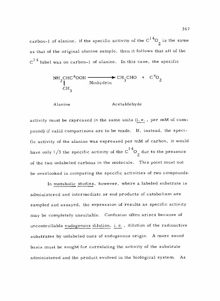
367
carbon -1 of alanine, if the specific activity of the C140 is the same 2
as that of the original alanine sample, then it follows that all of the
C14 label was on carbon -1 of alanine. In this case, the specific
NH CHC *OOH CH CHO + C 'O 21 Ninhydrin 3 2
CH3
Alanine Acetaldehyde
activity must be expressed in the same units (i. e. , per mM of com-
pound) if valid comparisons are to be made. If, instead, the speci-
fic activity of the alanine was expressed per mM of carbon, it would
14 have only 1/3 the specific activity of the C 02 due to the presence
of the two unlabeled carbons in the molecule. This point must not
be overlooked in comparing the specific activities of two compounds.
In metabolic studies, however, where a labeled substrate is
administered and intermediate or end products of catabolism are
sampled and assayed, the expression of results as specific activity
may be completely unsuitable. Confusion often arises because of
uncontrollable endogenous dilution, i. e. , dilution of the radioactive
substrates by unlabeled ones of endogenous origin. A more sound
basis must be sought for correlating the activity of the substrate
administered and the product evolved in the biological system. As
2
368
an example, consider the case where pyruvate -1 -C1 4 (100,000
cpm /mM of pyruvate) is administered to a rat. The substrate is de-
carboxylated and the recovered CO2 is found to have a specific acti-
vity of 10, 000 cpm /mM of CO2. This expression of results might
lead one to state that the pyruvate was only ten percent utilized by
the rat. However, this is not the whole story. It is necessary to
report also that the total recovery of CO showed an activity of
100,00 cpm. Thus, all of the activity was actually recovered in
respired CO2, but was greatly diluted by CO2 derived from other
substrates being simultaneously catabolized.
When specifically labeled substrates, such as glucose -1 -C14
14 and glucose -2 -C , are being administered to organisms in concur-
rent experiments, the effect of dilution is an even more serious
limitation on the expression of the results as specific activity of the
CO2 evolved. A direct comparison of the specific activities of the
14 14 CO2 derived from glucose -1 -C and from glucose -2 -C cannot be
made, since the CO2 is not evolved on the same basis in each case.
This difficulty can, however, be overcome to a certain extent by
the administration of glucose -U as the sole substrate in a con-
current experiment. The specific activity of the CO2 derived from
14 the glucose -U -C is then taken as a standard for the necessary
correction for endogenous dilution. Such a relative specific activity
2
2
2
369
allows cross comparisons and is of great value in determining the
probable pathways of metabolic interconversions.
A further complication of metabolic studies using specifically
labeled substrates is the randomization of the label due to re -entry
of the intermediate or end products of catabolism. The fixation of
CO by biological systems is perhaps the commonest type of re- 2
entry. For example, C140 derived from specifically labeled glu- e
cose may recombine with pyruvate to give malic acid. The labeling
pattern of this malic acid will differ from that of malic acid derived
directly from the original glucose. The malic acid formed by re-
entry of CO would then be further degraded through the tricarboxy- 2
lic acid cycle to yield CO with a different specific activity than that 2
derived directly from the original glucose.
d. Time -course studies - -- radiorespirometry: Because of
the confusion arising in many such metabolic experiments from the
expression of the results in specific activity, it has been found
more desirable to state results as percentage yield (total activity
in CO /total activity in labeled substrate). In addition, the radio - 2
respirometric method developed by Wang, et al. (7, p. 274-290,11)
permits a kinetic study of the metabolic sequences involved. This
method for metabolic pathway study calls for the collection at regu-
lar short intervals and assay of C1402 produced from a bank of 2
370
concurrent experiments. Each experiment represents a test or- 14
ganism which has been administered a substrate labeled with C at
a specific carbon atom. Information collected in an experiment of
this type is expressed as percent radiochemical recovery of the
labeled carbon atom in the respiratory CO2 per unit time. The
kinetics of the process are automatically displayed when one plots
the interval recoveries against time. Such a plot of data from ex-
periments with glucose catabolism in the microorganism Acetobacter
suboxydans is shown in Figure 10 -1.
The advantage in the use of the interval C O 14 yields lies
2
in the fact that they are not affected by endogenous dilution, thus
permitting one to trace the fate of a given carbon atom of a particu-
lar substrate in cellular respiration. Furthermore, the kinetic
feature of the radiorespirometric method allows one to examine the
progress of an experiment if a rapid counting technique, such as
liquid scintillation counting, is used for the assay of the radioacti-
vity in the respired CO . With proper experimental design, it is 2
therefore possible to trace the complete biological fate of a given
substrate, i. e. , complete utilization of the administered substrate
with respect to all catabolic pathways.

100
80 Glucose -1 -C14
Glucose -2 -C 14
- - - - --- Glucose -3, 4 -C14 Glucose-6-C"
0 1 2 3 4 5
Time in Hours
Figure 10 -1. Time -course plot of radiochemical recovery in CO2 from Acetobacter suboxydans metabolizing specifically labeled glucose.
- -' -
u,
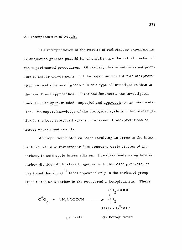
372
2. Interpretation of results
The interpretation of the results of radiotracer experiments
is subject to greater possibility of pitfalls than the actual conduct of
the experimental procedures. Of course, this situation is not pecu-
liar to tracer experiments, but the opportunities for misinterpreta-
tion are probably much greater in this type of investigation than in
the traditional approaches. First and foremost, the investigator
must take an open- minded, unprejudiced approach to the interpreta-
tion. An expert knowledge of the biological system under investiga-
tion is the best safeguard against unwarranted interpretations of
tracer experiment results.
An important historical case involving an error in the inter-
pretation of valid radiotracer data concerns early studies of tri-
carboxylic acid cycle intermediates. In experiments using labeled
carbon dioxide administered together with unlabeled pyruvate, it
was found that the C14 label appeared only in the carboxyl group
alpha to the keto carbon in the recovered o(- ketoglutarate. These
CH -COOH I 2
J.
C 02 + CH3COCOOH y CH2 I
0 = C - C *OOH
pyruvate oc.- ketoglutarate
T

373
results were interpreted to mean that a symmetrical molecule like
citric acid could not be in the pathway from pyruvate to i.- ketoglu-
tarate, because randomization of the label would otherwise occur.
Thus, citric acid was ruled out as an intermediate in the sequence
of reactions often called the citric acid cycle! However, Ogston
postulated that if the substrate were attached to an enzyme surface
at three points which are catalytically different, then it might pass
through the stage of a symmetrical intermediate (citric acid) and
then be converted to the unsymmetrical compound without randomi-
zation of the label. This hypothesis was subsequently verified by
further radiotracer studies and citric acid restored to its rightful
place as a tricarboxylic acid cycle intermediate. Note that the
radiotracer data were unchanged through all of this discussion.
Only the interpretation of results had changed.
Another common error of interpretation is the failure to
recognize that one is following the label, not the administered com-
pound. Again, one may not find the label in the end product be-
cause unexpected dilution has reduced its specific activity below
the detection limits of the assay system. Such negative results
must be checked by repeating the experiment with a higher specific
activity. In line with this problem, the precision of the experiment
must be clearly understood and stated. It is obviously ridiculous to
374
to state results of 1 dpm! All the steps in the experiment, not only
those involving radioactivity assay, must be evaluated for their ef-
fect on overall precision.
Finally, one must be alert to the presence of artifacts in
experimental results. These may result from such causes as chem-
ical or radiochemical contaminants in the original tracer dose. In
liquid scintillation counting, excessively high count rates may be
the result of chemiluminescence (see p. 285) and entirely unrelated
to counting sample activity. Autoradiography is particularly prone
to artifacts (see p. 244 -245). Levi (5) has recently reported a
unique artifact in the autoradiography of leaves of bean plants con-
taining P32. He showed that the apparent accumulation of isotope
in primary leaves that were oven -dried prior to exposure to x -ray
films was not metabolic, but due to a drying gradient occurring
within the leaves. This artifact disappeared when autoradiographs
were made of leaves that had been freeze -dried under vacuum.
This illustrates the unexpected sources of artifacts.
In this chapter it has only been possible to highlight the
basic features and problems of radiotracer experimental design.
The task of applying these generalities to particular biological ex-
periments must lie with the reader.
375
BIBLIOGRAPHY
1. Bowen, H. J. M. Biological fractionation of isotopes. The International Journal of Applied Radiation and Isotopes 7:261 -272. 1 960.
2. Cohn, Waldo E. Radioactive contaminants in tracers. Analytical Chemistry 20:498 -503. 1948.
3. Lax, Louis C. and Gerald A. Wrenshall. Measurement of turn- over rates in systems of hydrodynamic pools out of dynamic equilibrium. Nucleonics 11 (4):1 8 -20. 1953.
4. Lemmon, Richard M. Radiation decomposition of carbon-14 - labeled compounds. Nucleonics 11(10):44-45. 1 953.
5. Levi, A. An artifact in plant autoradiography. Science 137: 343-344. 1 962.
6. Rabinowitz, Joseph L. , et al. Carbon isotope effects in enzyme systems. I. Biochemical studies with urease. Archives of
Biochemistry and Biophysics. 63:437 -445. 1956.
7. Rothchild, Seymour (ed. ). Advances in tracer methodology, vol. 1. New York, Plenum Press, 1963. 332 p.
8. Sheppard, C. W. Basic principles of the tracer method. New York, John Wiley, 1962. 282 p.
9. Stokinger, Herbert E. Size of dose: its effect on distribution in the body. Nucleonics 11 (4):24 -27. 1 953.
10. Tolbert, Bert M. Self- destruction in radioactive compounds. Nucleonics 1 8(8):74 -75. 1 960.
11. Wang, C. H. , et al. Comparative study of glucose catabolism by the radiorespirometric method. Journal of Bacteriology 76:207 -216. 1958.
12. Wilson, E. Bright, Jr. An introduction to scientific research. New York, McGraw -Hill, 1952. 375 p.

376
13. Zilversmit, D. B. and Moris L. Shore. A hydrodynamic model of isotope distribution in living organisms. Nucleonics 10(10): 32 -34. 1952.

377
CHAPTER 11 - AVAILABILITY OF RADIOISOTOPE COMPOUNDS
The investigator proposing to use radiotracer methods is
faced with the practical problem of securing suitable radioisotope
compounds. Most frequently this problem is resolved by purchasing
the already labeled compounds from a commercial radiochemical
supplier. In some cases the desired tracer compound may not be
commercially available and synthesis must be attempted. In either
case it is important to have some conception of the problems of pri-
mary radioisotope production and conversion of the primary product
to an experimentally useful radiotracer compound. In this chapter
a brief survey of these steps will be given, although these considera-
tions are primarily in the province of the radiochemist.
A. Primary Production of Radioisotopes
1. Nuclear reactor production
The artificial production of radioisotopes has already been
considered in some detail in Chapter 1 (p. 24 -30). It will be recalled
that the nuclear reactor is the most generally useful production
source of artificial radioisotopes. The commonest production me-
thod utilizes the neutron irradiation in a reactor to bring about nu-
clear alteration in specific target atoms, for example (n, Y ), (n, p),
or (n, a) reactions. The problem of the (n, Y ) process with regard

378
to the specific activity of the product has already been discussed
(p. 29) The advantage afforded by the Szilard- Chalmers reaction in
allowing the attainment of high specific activities in the product of
certain (n, Y ) processes should again be mentioned. This reaction
is further described in Experiment V, where it is used to produce
radioactive 1128 from stable I127.
Most of the fragments of the uranium atoms which have under-
gone fission in the reactor are radioactive atoms ranging from atomic
numbers 30 through 64. These fission products can be concentrated
chemically to high specific activities, but since several isotopes of
any one element are often produced, the isotopic purity will not neces-
sarily be as high as that of radioisotopes produced by (n, p ) and
(n, a) processes.
In the United States the principal source of primary radio-
isotope material is from the reactors at the Oak Ridge National
Laboratory of the U. S Atomic Energy Commission. In England,
the Radiochemical Centre at Amer sham and Harwell serves a simi-
lar function and in addition supplies a wide variety of labeled com-
pounds. Some small scale reactor production of specific isotopes
is carried on by commercial firms.
The radioactive products of neutron irradiation or fission,
as they come from the reactor, must be chemically processed. The

379
processed isotopic materials are most generally sold as simple in-
organic compounds or in elementary form. Table 11 -1 lists all the
radioisotopes currently available from the Oak Ridge National
Laboratory, in order of increasing half -life. (Those with half -lives
of less than one hour are omitted. ) Data on the maximum specific
activities available, type of radiation emitted, and production me-
thod are also noted. The wide variation in specific activities avail-
able from isotope to isotope has implications as to their suitability
for radiotracer purposes (p. 36]. Further information on these pri-
mary radioisotopes can be found in the Oak Ridge National Laboratory
Catalog and Price List of Radioisotopes (12). It should be mentioned
that Oak Ridge, as well as many commercial firms operating re-
actors, will perform service irradiation of materials on a custom
basis.
2. Cyclotron production
The cyclotron is a generally more versatile device for pro-
ducing radioisotopes than the nuclear reactor because of the wider
variety and energy of the accelerated nuclear particles it can employ.
It has been previously pointed out that deuterons are the most useful
charged particles for bringing about transmutation (p. 25), but, in
addition, electrons, alpha particles, protons, or heavy ions (such
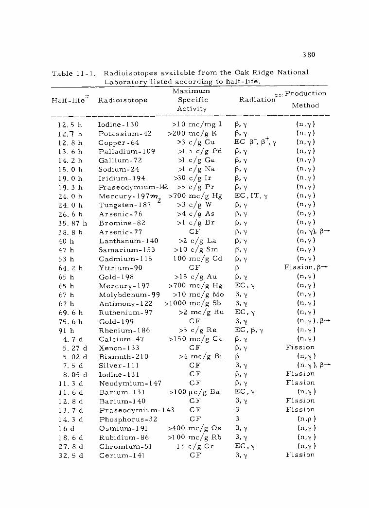
380
Table 11 -1. Radioisotopes available from the Oak Ridge National Laboratory listed according to half -life.
Half -life' Maximum
Radioisotope Specific Activity
r; Production Radiation"
12.5 h Iodine -130 >10 me /mg I ß, Y (n,Y) 12.7 h Potassium -42 >200 mc/g K ß,Y (n,y) 12. 8 h Copper -64 >3 c/g Cu EC ß,ß±Y (n,y) 13. 6 h Palladium -109 >1.5 c/g Pd ß, Y (no() (n,y) 14. 2 h Gallium-72 >1 c/g Ga P, Y
15. 0 h Sodium -24 >1 c/g Na P., (n,y) 19. 0 h Iridium -194 >30 c/g Ir ß. Y (n,y) 19. 3 h Praseodymium -142 >5 c/g Pr ß Y
24. 0 h Mercury -197-nß >700 mc/g Hg 2
EC, IT, Y (n,y) 24. 0 h Tungsten -187 >3 c/g W ß Y (n,Y) 26. 6 h Arsenic -76 >4 c/g As P.,
35. 87 h Bromine -82 >1 c/g Br P, (n,Y) 38. 8 h Arsenic -77 CF ß Y
(n, Y), ß-' 40 h Lanthanum -140 >2 c/g La P, (n,Y )
47 h Samarium -153 >10 c/g Sm P, Y (n,y) 53 h Cadmium-115 100 mc/g Cd ß, 64. 2 h Yttrium -90 CF ß Fission, p-- 65 h Gold -198 >15 c/g Au ß, Y (n,Y )
65 h Mercury -197 >700 mc/g Hg EC, -y (n,Y )
67 h Molybdenum -99 >10 mc/g Mo ß Y (n,./) 67 h Antimony -122 >1000 mc/g Sb P, (n,y) 69. 6 h Ruthenium -97 >2 mc/g Ru EC, .¡
75. 6 h Gold -199 CF P., Y (n,Y 91 h Rhenium -186 >5 c/g Re EC, ß,Y (n,Y )
4. 7 d Calcium -47 >150 mc/g Ca ß, Y (n,Y )
5. 27 d Xenon -133 CF ß, Fission 5. 02 d Bismuth -210 >4 mc/g Bi ß (n,y) 7. 5 d Silver -111 CF ß. Y
(n,Y
8. 05 d Iodine-131 CF ß, Fission 11. 3 d Neodymium -147 CF ß, Y Fission 11. 6 d Barium -131 >100 µcg Ba EC, Y (n,Y )
12. 8 d Barium -140 CF ß, Fission 13. 7 d Praseodymium -143 CF ß Fission 14. 3 d Phosphorus -32 CF (n,p )
16 d Osmium -191 >400 mc/g Os ß, Y (n,Y )
18. 6 d Rubidium -86 >100 mc/g Rb ß, Y (no/ )
27. 8 d Chromium -51 15 c/g Cr EC, (n,y )
32.5 d Cerium -141 CF p, Fission
(n,y) Y
(n,y)
Y (n,y) Y
(n,y)
Y
(n,y)
ß- Y
ß
Y
Method
y
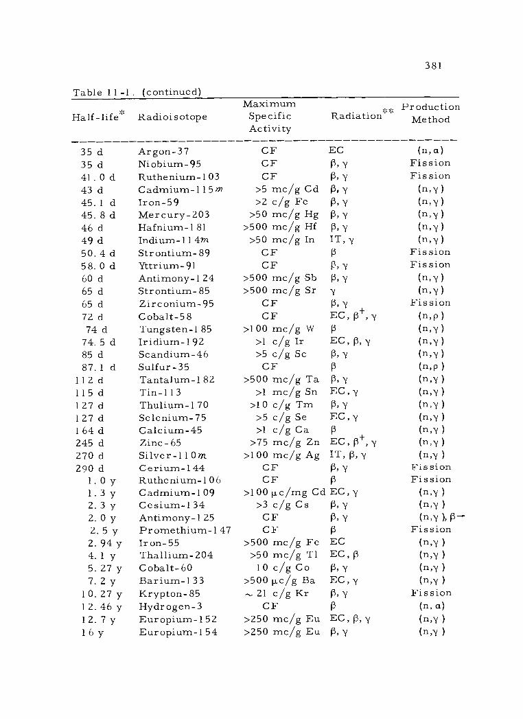
381
Table 1 1 -1 . (continued) Maximum Production
Half-life Radioisotope Specific Radiation Method Activity
35 d Argon -37 CF EC (n, a) 35 d Niobium-95 CF p, Y Fission 41. 0 d Ruthenium -1 03 CF p, Fission 43 d Cadmium-115m >5 mc/g Cd (3, y (n,y) 45. 1 d Iron -59 >2 c/g Fe p, (n,y )
45. 8 d Mercury -203 >50 mc/g Hg 13, Y (n,y (n,y )
46 d Hafnium -1 81 >500 mc/g Hf p, y (n,y) 49 d Indium-11 47n >50 mc/g In IT, y (n,y )
50. 4 d Strontium-89 CF p Fission 58. 0 d Yttrium-91 CF p, Fission 60 d Antimony -1 24 >500 mc/g Sb p, y (n,y) 65 d Strontium-85 >500 mc/g Sr Y (n,y )
65 d Zirconium -95 CF p, Fission 72 d Cobalt -58 CF EC, p+, Y (n,P )
74 d Tungsten -1 85 >100 mc/g W p )
74. 5 d Iridium -1 92 >1 c/g Ir EC, p, (n,y )
85 d Scandium -46 >5 c/g Sc ß, (n,y )
87. 1 d Sulfur -35 CF p (n,p )
112 d Tantalum -1 82 >500 mc/g Ta P, y (n,y )
115 d Tin-113 >1 mc/g Sn EC, Y (n,-y )
127 d Thulium -1 70 >1 0 c/g Tm p, y (n'Y )
127 d Selenium - 75 >5 c/g Se EC, y (n,y )
1 64 d Calcium -45 >1 c/g Ca P (n,y )
245 d Zinc-65 >75 mc/g Zn EC, p+, Y (n,y )
270 d Silver -110m >1 00 mc/g Ag IT, p, y (n,y) 290 d Cerium -144 CF p,y Fission
1. 0 y Ruthenium -1 06 CF p Fission 1.3 y Cadmium -1 09 >100 µ.c/mg Cd EC, y (n,y )
2. 3 y Cesium -134 >3 c/g Cs p,y (n,y )
2. 0 y Antimony -1 25 CF p, y (MY ), p 2. 5 y Promethium -1 47 CF p Fission 2. 94 y Iron-55 >500 mc/g Fe EC (n,Y )
4. 1 y Thallium-204 >50 mc/g T1 EC, p (n,y )
5. 27 y Cobalt-60 1 0 c/g Co ß, y )
7. 2 y Barium -1 33 >500 µc/g Ba EC, y (n,y) 1 0. 27 y Krypton-85 -.. 21 c /g Kr P,y Fission 1 2. 46 y Hydrogen -3 CF p (n, a) 1 2. 7 y Europium -1 52 >250 mc/g Eu EC, p, y (n,y )
1 6 y Europium -1 54 >250 mc/g Eu p, (n,y )
Y
Y
y
y
y
y
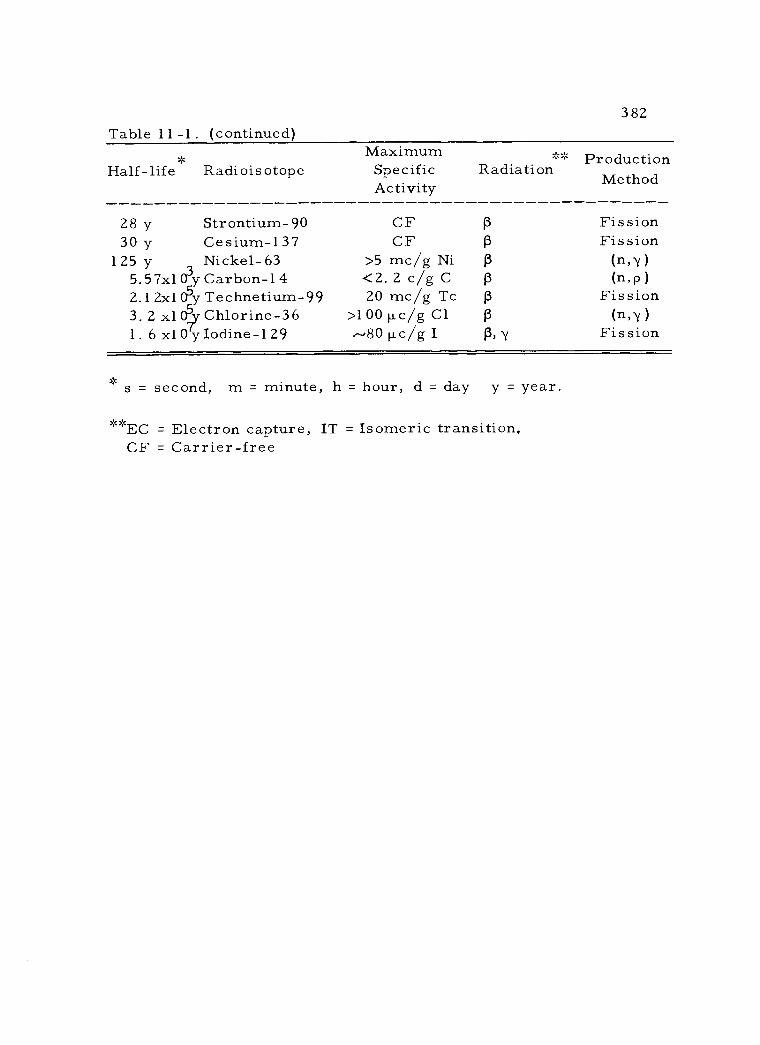
382 Table 11 -.1. (continued)
Maximum Half -life Radioisotope Specific Radiation Production
Activity Method
28 y Strontium -90 CF f3 Fission 30 y Cesium -137 CF f3 Fission
125 y Nickel -63 >5 mc/g Ni f3 (no') 5.5 7x1 03y Carbon-1 4 <2. 2 c/g C ß (n, p )
2.1 2x1 05y Technetium -99 20 mc/g Tc ß Fission 3. 2 x1 055y Chlorine -36 >1 00 µc/g Cl ß (n,Y )
1. 6 xl 0 y Iodine -1 29 .80 µc/g I ß, Y Fission
s = second, m = minute, h = hour, d = day y = year.
J. w **EC = Electron capture, IT = Isomeric transition,
CF = Carrier -free
wT
*
383
3+ as N ) may be used in the cyclotron. However, operating costs for
cyclotrons are so much greater than those for nuclear reactors, that
the former are employed for radioisotope production only when they
offer a significant advantage over reactors.
A major advantage of the cyclotron is that certain useful
radioisotopes may be produced in it which are not produced in signi-
ficant quantities in nuclear reactors. Some examples of isotopes in
this category are Bel, Na22, A126, V48, V49, Mn54, and As74. In
the case of A126, V48, V49, and Mn54, these are the only isotopes
of their elements suitable for use as radiotracers. An additional
advantage is that, in many cases, radioisotopes may be produced
with much higher specific activities (frequently carrier -free) in the
cyclotron than in nuclear reactors. Certain radioisotopes cannot be
produced free of other radioisotopes of the same element in a reac-
tor without resorting to very expensive highly enriched target ele-
ments. However, by means of the cyclotron it has been possible to
prepare Fe55 free of Fe59 , and Sr85 free of Sr89 and Sr90
B. Conversion of Primary Radioisotopes to Experimentally Useful Compounds
In certain experiments the primary radioisotopes may be
employed directly, but most frequently the investigator will desire
to secure a more complex labeled compound for use in radiotracer
384
experiments involving living organisms. A compound that is either
randomly labeled or uniformly labeled (such as glucose- U -C14) may
suffice for the purpose of one particular experiment, while a speci-
fically labeled compound (such as glucose- 2 -C14) may be required
in other investigations. Since the great preponderance of labeled
compounds used in biological tracer studies are C14- tagged, the
following discussion will deal largely with carbon-1 4 labeling. Gen-
erally, atoms of the radioisotope (C14) may be introduced into the
molecules to be labeled either by chemical synthesis or biosynthesis.
In the case of tritium, certain unique methods of labeling are pos-
sible.
1. Chemical synthesis
A carbon -14 label may be introduced into a wide variety of
compounds by the standard synthetic procedures of organic chemis-
try. (The same generally applies to P32, S35, and I131 labels). In
addition, some completely new methods have been devised in order
to conserve the labeling radioisotope. It would not be feasible here
to list all the possible syntheses that have been used. Calvin, et al.
(1 , p. 148-239), have devoted a large portion of their volume to a
general survey of the synthetic routes used in producing C14- labeled
compounds. Kamen (6, p. 311-332) has presented in tabular form an
385
extensive list of specific syntheses for labeling with carbon -14. In
addition, a more recent work by Murray and Williams (9) covers
this field in an encyclopedic manner. Part 1 of their volume deals
with carbon labeling, while Part 2 is concerned with halogen (I, Cl,
Br), tritium, P32 and S35 compounds.
Chemical synthesis of labeled compounds suffers from several
limitations and problems. One limitation is the amount and cost of
the isotopic starting material available. This factor necessitates
devising synthetic routes to the desired compounds in which the ra-
dioisotopic label can be introduced near the end of the sequence of
reactions, so as to secure as high an overall yield of labeled mate-
rial as possible. Since the syntheses will normally be carried out
on a micro or semimicro scale, losses due to transfer may be great
and overall yield consequently low. At present, a great diversity of
labeled compounds are available commercially as starting materials
for syntheses. Still, it is necessary in planning a new synthetic
route to consider its compatability with the specific starting mate-
rial available. Yet another disadvantage of chemical synthesis is
that when it is used to produce certain biologically important com-
pounds, such as amino acids, a mixture of D- and L- isomers re-
sults. These are not separable chemically. Since organisms meta-
bolize the L -form selectively (in the case of amino acids), the use

386
of such racemates in biological investigations is somewhat unphysio-
logical. The greatest drawback of chemical synthesis is that there
are many compounds of biochemical importance which cannot be
synthesized in the laboratory by the classical methods of organic
chemistry.
2. Biosynthesis
Living organisms, or their enzyme extracts, offer a means
of synthesizing certain labeled compounds not obtainable by chemi-
cal synthesis. These include both the macromolecules (proteins,
polysaccharides, nucleic acids, etc. ) and many simpler molecules
(vitamins, hormones, amino acids, sugars). The successful employ-
ment of biosynthesis for production of a given labeled tracer corn-
pound is dependent on several factors. First, an organism must be
selected that will synthesize and accumulate practical quantities of
the desired compound. Culture conditions must be established to
provide optimal yields of the highest specific activity. Last, and
most important, procedures must be established for isolating and
purifying the labeled compound, and determining the distribution
pattern of the label.
Photosynthetic methods offer the advantage of using the rela-
tively inexpensive C1402 (from BaC1403) as the starting material.
387
Carbon -14 labeled starch, glucose, fructose, and sucrose can be
isolated in gdod yields from green leaves or algal suspensions that
have been exposed to a C 14
O atmosphere and illuminated for several 2
days. Specific activities of up to 200 me /mM of glucose -U -C14 have
recently been achieved in such biosyntheses. Similarly, green algae
of the genus Chlorella can be used to produce C14- labeled amino
acids.
Microorganisms, or their enzyme extracts, have been used 14
to produce organic acids tagged with C , either by direct synthesis
or transformation of labeled substrates. Several species of micro-
organisms have been used to produce higher fatty acids by condensa-
tion. Calvin, et al. (1 , p. 262 -277), describe some of the specific
biosyntheses that have been generally used.
The distribution of label resulting from biosynthesis of a
given compound varies according to the conditions of the synthetic
reaction. All the carbon atoms of a compound are not labeled with
C14 at the same rate. Under certain conditions, all the atoms in a
given compound may be labeled, but not to the same extent. Such a
compound is described as generally, or totally labeled. If the label-
ing is such that the specific activity of each carbon atom in the com-
pound is essentially equal, the compound is uniformly labeled (such
as glucose- U -C14). Such uniform labeling requires that the
388
organism be in equilibrium with the substrate. Specifically labeled
compounds (such as glucose -1 -C14) are available at generally lower
specific activities than their uniformly labeled counterparts.
In most situations the biological investigator will prefer to
secure labeled compounds from commercial sources. The radio-
chemical purity of such compounds cannot be assumed. Radiation
induced self -decomposition can result in the accumulation of labeled
degradation products which must be removed before experimental
use. Reputable radiochemical suppliers will furnish chromatogra-
phic evidence of compound purity, but, nevertheless, purification of
the compound should be the initial step in any radiotracer experi-
ment.
The most complete guide to the commercially available la-
beled compounds is the Isotope Index (17). It lists hundreds of C14
tagged compounds, as well as those labeled with I131, P32, S35
and H3. In addition, the various radiochemical supply house cata-
logs should be consulted for the most up -to -date information on
compound availability.
3. Tritium labeling
Tritium labeled compounds have received increasing use in
recent years (20), in spite of the fact that the mean energy of beta
389
emission from H3 is only about 5. 5 Key. This increased attention
is due largely to the development of improved methods of tritium
labeling and the application of liquid scintillation counting to tritium
assay. Since carrier -free tritium gas can be obtained, very high
3 specific activities in H -labeled tracer compounds are attainable.
Commercially available compounds (such as thymidine, tryptophan,
epinephrine, etc. ) can be secured with specific activities of 4 - 6
curies /mM when the label is tritium, whereas C14- labeled corn-
pounds are usually available only at specific activities of a few mc/
mM. So important has tritium usage become that in recent years
several symposia have been convened on the subject (4, 10, 1 1 ).
Compounds may be labeled with tritium by several methods
(14). The classical synthetic methods utilizing labeled intermedi-
ates (as described above) have the advantage of yielding products
that have predictable specific activities, are specifically labeled,
and have a minimum of tagged byproducts. The disadvantages of
synthesis are cost and the limitation on the variety of compounds
that can be successfully labeled. For this reason, many compounds
are labeled by one of several unique methods.
a. By reduction of unsaturated precursors: The method of
choice for labeling with tritium is the reduction of a suitable unsa-
turated precursor (containing a double bond, carbonyl group, etc. )

390
with carrier -free tritium gas. The major limitation of this method
is the availability of a suitable unsaturated precursor of the desired
compound. It is essential to carry out the reduction in a non- hydroxy-
lic solvent (dioxane, ethyl acetate, etc. ). Reductions carried out in
alcohol or water will lead to almost complete exchange of the tritium
gas with the solvent. Careful purification of the product is required,
since competing reactions may also occur. The advantages of this
method are the very high specific activities attainable, the purity of
the product, and the known position of labeling.
b. By exchange reactions: Random tritium labeling may be
secured by simple exchange methods, with or without catalytic ac-
tion. For example, the simple exchange of tritiated water (THO)
with the labile hydrogen of malonic acid, followed by decarboxylation,
yields tritiated acetic acid. In catalyzed exchanges, either tritiated
water or glacial acetic acid (CH3COOH3) is the usual medium and
platinum black the commonly used catalyst. This method is only
suitable for compounds which are stable in aqueous solution at tem-
peratures up to 120° C.
Although high specific activities may be obtained by this me-
thod, much of the introduced tritium will be labile. Removal of this
labile tritium and purification of the desire product is a troublesome
necessity. One gram of compound can be expected to have perhaps

391
40 - 400 me of non - labile tritium associated with it. In general, the
labeled product is of higher purity and specific activity than that from
the gas exposure method (see below), and complete purification is
easier.
c. By gas exposure: The work of Wolfgang and Rowland (1 6,
26) in the mid-1 950's involving tritium - recoil labeling of organic 3
compounds laid the foundation for a new method of H -labeling.
Wilzbach (24), in 1 957, first described the simplified approach to
random labeling with tritium that has come to be called the Wilzbach
gas- exposure method and is largely responsible for the increased
popularity of tritium as a tracer. In this method, the compound to
be labeled is exposed to curie amounts of carrier -free tritium gas in
a sealed reaction vessel for a period of a few days to several weeks.
The energy released in the disintegration of the tritium and absorbed
by the system provides the activation necessary to effect labeling.
Wilzbach reported that specific activities of 1 - 1 25 me /gram of
purified compound have been obtained (15, p. 4 -11 , 28 -31 ).
Unfortunately, Wilzbach labeling is accompanied by the form-
ation of tritiated by- products of high specific activity. As in the
case of exchange labeling (see above) a considerable portion of the
tritium in the labeled compound is often labile. Nystrom and
Dutton (15, p. 1 8 -27, 46 -49) have shown that addition of tritium to
392
unsaturated molecules accompanies the labeling process to a greater
or lesser degree, depending on the nature of the double bond. This
formation of labeled by- products is the major problem of the gas -
exposure method. Although it is easy to remove contaminants with
molecular weights different from that of the parent compound (such
as those formed by fragmentation or polymerization), it is difficult
to remove contaminants formed by hydrogenation, racemization, or
isomerization. Thus, rigid purification procedures must be followed.
Modifications of the Wilzbach method have used external
energy to accelerate the labeling process. Electric discharge through
the reaction vessel has been widely employed (2, 5, 7, 22, 25).
Microwaves (3), ultraviolet irradiation, and gamma irradiation have
also been used. All of these techniques increase the rate of incor-
poration and allow faster labeling with smaller amounts of tritium
gas, but in many instances they lead to an increase in labeled degra-
dation products. Mottlau (8) suggests that the addition of argon or
helium gas to the reaction vessel atmosphere will reduce this com-
peting decomposition.
The chief advantage of the gas- exposure method is that it
permits the labeling of compounds of complex or even unknown
structure which cannot be readily labeled in any other way (1 5,
p. 32 - 41). As examples, insulin (21), digitoxin (1 8), and a
393
variety of proteins (19) have been successfully tagged. Whisman
and Eccleston (23) at the conclusion of their excellent review of the
gas- exposure method list preparative data on 1 38 different tritium
labeled compounds. However, because of the magnitude of the puri-
fication procedure required and the random nature of the labeling,
it is suggested that all other synthetic routes be explored before the
gas- exposure method is chosen.
BIBLIOGRAPHY
1. Calvin, Melvin, et al. Isotopic carbon. Techniques in its measurement and chemical manipulation. New York, John Wiley, 1949. 376 p.
2. Dorfman, Leon M and Kenneth E Wilzbach. Tritium labeling of organic compounds by means of electric discharge. The Journal of Physical Chemistry 63:799 -801. 1959.
3. Chanem, N. A and T. Westermark. Extensions of the tech- niques for the accelerated unspecific isotopic labelling of organic compounds. In: Radioisotopes in the physical sciences and industry. vol. 3. Vienna, International Atomic Energy Agency, 1962. p. 43 -67.
4. International Atomic Energy Agency. Proceedings of the Sym- posium on the Detection and Use of Tritium in the Physical and Biological Sciences, Vienna, 1961. vol. 2. Vienna, 1962. 438 p.
5. Jackson, Frank L , George W. Kittinger and Frank P. Krause. Efficient tritium labeling with an electric discharge. Nucleonics 18(8):102 -105. 1960.

394
6. Kamen, Martin D Isotopic tracers in biology. An introduction to tracer methodology. 3d ed. New York, Academic Press, 1957. 478 p.
7. Lemmon, Richard M. , et al. Ionizing energy as an aid in ex- change tritium labeling. Science 129 :1740 -1741. 1959.
8. Mottlau, A Y. Effect of a noble gas on the labeling of n- hexane by exposure to tritium. The Journal of Physical Chemistry 64:931 -933. 1960.
9. Murray, Arthur, III and D Lloyd Williams. Organic syntheses with isotopes. New York, Interscience, 1958. 2096 p.
10. New England Nuclear Corp. Proceedings of the Symposium on Tritium in Tracer Applications, New York, 1957. Boston, 1958. 40 p.
11. . Proceedings of the Symposium on Ad- vances in Tracer Applications of Tritium, New York, 1958. Boston, 1959. 67 p.
12. Oak Ridge National Laboratory. Catalog and price list of radio- isotopes, special materials and services. 3d ed. Oak Ridge, 1960. 196 p.
13. Pearlman, William H. A method for labeling C21 and C19 3 steroid hormones with tritium at C -7: progesterone -7 -H
and 4- androstene -3, 17- dione -7 -H. The Journal of Biological Chemistry 236:700 -704. 1961.
14. Rosenblum, Charles. The chemistry and application of tritium labeling. Nucleonics 17(12):80 -83. 1959.
15. Rothchild, Seymour. (ed.) Advances in tracer methodology. vol. 1. New York, Plenum Press, 1963. 332 p.
16. Rowland, F S. and Richard Wolfgang. Tritium -recoil labeling of organic compounds. Nucleonics 14(8):58 -61. 1956.
17. Sommerville, J. L. (ed. ). The isotope index. vol. 6. Indianapolis, Scientific Equipment Co. , 1962. 206 p.
395
18. Spratt, James L. , George T Okita and E. M Geiling. In vivo radiotracer stability of a tritium "self- radiation" - labeled compound. The International Journal of Applied Radiation and Isotope 2:167 -168. 1957.
19. Steinberg, D , et al. Preparation of tritiated proteins by the Wilzbach method. Science 126:447 -448. 1957.
20. Tritium tracing -- a rediscovery. Nucleonics 16(3):62 -67. 1958.
21. Von Holt, C. , I. Voelker and L. Von Holt. Markiering von Insulin mit Tritium. Biochimica et Biophysica Acta 38:88- 101. 1960.
22. Westermark, Torbjorn, Hans Linroth and Bengt Enander. Isotope labelling by means of electrical gaseous discharges. The International Journal of Applied Radiation and Isotopes 7:331 -334. 1960.
23. Whisman, Marvin L and Barton H Eccleston. Gas - exposure labeling of organics with tritium. Nucleonics 20(6):98 -105. 1962.
24. Wilzbach, Kenneth E. Tritium -labeling by exposure of organic compounds to tritium gas. Journal of the American Chemical Society 79:1013. 1957.
25. Wilzbach, K. E. and L. M. Dorfman. Labelling of organic compounds by electric discharge in tritium gas. In: Radio- isotopes in the physical sciences and industry. vol. 3. Vienna, International Atomic Energy Agency, 1962. p. 3 -11.
26. Wolfgang, Richard, F. S. Rowland and C. Nigel Turton. Production of radioactive organic compounds with recoil tritons. Science 121:715 -717. 1955.

396
CHAPTER 12 - SAFE HANDLING OF RADIOISOTOPES
The deleterious effects of ionizing radiation on living organ-
isms were recognized quite early in its usage and are well known
today (11). In certain situations (as in cancer therapy or radiation
sterilization of food) these damaging effects are employed for man's
benefit. However, the investigator using radioactive tracers is con-
cerned with avoiding the potential biological effects of their radia-
tions. In the United States, the Atomic Energy Commission has
taken primary responsibility with regard to hazards arising from
the use of radioisotopes. To this end, carefully worded federal
rules and regulations governing the use of radioisotopic materials
have been put in force (14). In addition, useful reference material
dealing with all aspects of radiation safety is found in the handbooks
by Blatz (3) and Kinsman (9).
The problems involved in the safe handling of radioactive
isotopes can be classified into three categories. These are: (1)
protection of personnel, (2) control of contamination, and (3) dis-
posal of radioactive waste. It should be stressed at this point that
in the use of tracer amounts of all but the most hazardous radioiso-
topes the most pressing problem is the avoidance of technical con-
tamination of the laboratory environment. Such technical
397
contamination will usually render a laboratory useless for further
tracer work well before an actual health hazard exists (4). Thus,
the radiotracer user must constantly practice good housekeeping.
However, even though only tracer levels of activity are being used
experimentally, higher levels of activity are commonly purchased
and must be handled initially. It should be emphasized that the pur-
pose of all radiation safety procedures is to keep radiation exposure
to a minimum. The permissible levels of radiation exposure that
have been established (14, 21) are conservative, but still to some
degree arbitrary.
A. Units of Radiation Exposure and Dose
In order to adequately discuss radiation hazards, it is neces-
sary to consider the units used to denote the energy involved. This
energy may be viewed either from the standpoint of radiation expo-
sure or the energy absorbed by material from the radiation incident
on it. It is the absorbed radiation dose that determines the biologi-
cal effects of the radiation. Unequivocal statements of radiation
dose or exposure must take into account the area involved and the
time factor, as well as the actual energy of the ionizing radiation
that is dissipated in the absorber. Thus, dose -rate and exposure -
rate must be stated and the portion of the body affected defined
398
(i. e. , whole body, hands only, etc. ). A good, general survey of
this whole topic of radiation biophysics will be found in the volume
by Andrews (2).
1. The roentgen
The most widely used unit of radiation exposure, the roentgen
(named after the discoverer of x- rays), is defined by the ionization
in air it produces. The roentgen (abbreviated r) was officially de-
fined by the International Radiological Congress at Chicago in 1937
as the quantity of gamma or x- radiation such that the associated
corpuscular emission per 1 cc of air at STP produces, in air, ions
carrying one electrostatic unit of quantity of electricity of either
sign. If this amount of charge is liberated in air, the energy ab-
sorbed by the air is approximately 87. 6 ergs /gram. In health
physics work, the exposure rate is commonly expressed in units of
roentgens per hour (r /hr) or milliroentgens per hour (mr /hr).
Unfortunately, the roentgen is only valid for photon interaction with
air, and cannot be applied to particulate radiation or tissue absorp-
tion. Notice also, that the roentgen is a measure of radiation ex-
posure, not dose, contrary to common misuse.

2. The rad
399
From the biological standpoint, interest centers primarily on
the energy absorbed by tissues rather than by air. Although the
roentgen had become universally used by medical workers, it was felt
necessary to devise an unambiguous unit of tissue dose that was not
necessarily related to it. The International Commission on Radiolo-
gical Units in 1953 proposed a new unit for absorbed dose called the
rad. It was defined as 100 ergs of energy imparted by any ionizing
radiation per gram of irradiated material at the place of interest.
Since the absorption of various materials differs, it is necessary to
state the medium considered when quoting doses in rads. The rad is
now the unit of choice when tissue absorption is considered. It has
generally replaced the rep (roentgen equivalent physical), which had
been invented as a dose unit for radiation other than gamma or x -rays.
3. The RBE, rem, and LET
It is evident that radiations of various types exhibit different
biological effects and that the overall biological damage to a system
is dependent on the type and energy of the radiation. For this rea-
son the relative biological effectiveness (RBE) of the radiation ab-
sorbed must be considered. RBE values are stated as the ratio of

400
the energy absorbed from gamma or x -rays to that absorbed by the
radiation in question which produces the same biological effect. On
this basis, the following average RBE values may be cited: gamma
rays, x -rays, beta particles -- RBE 1; thermal neutrons -- RBE
2. 5; fast neutrons, alpha particles, protons -- RBE 10; heavy ions --
RBE 20.
The unit of relative dose is the roentgen equivalent man (or
mammal), abbreviated rem. This is defined as the biologically ef-
fective dose which is equivalent in man to an exposure of one roent-
gen of gamma or x -rays. Thus, it will be seen that if the absorbed
dose in rads is multiplied by the RBE value of the radiation in ques-
tion, the result is the relative dose in rems.
It is believed that the density of ionization along a particle's
path is the primary factor which determines the biological effect.
Thus, is introduced the linear energy transfer (LET) unit, which is
a measure of the rate at which energy is dissipated in a system along
its path length. LET is commonly stated in Kev %µ. Values range
from less than 3. 5 for x -rays to well over 100 for heavy ionizing
particles.
B. Hazard Factors in Handling Radioisotopes
Many facets of radioactivity that relate to radiation safety
401
have already been discussed in this volume. The reader should now
be aware of the factors which cause certain radioisotopes to be more
hazardous than others. These include: (1) physical half -life, (2)
e iergy and type of radiation, (3) biological half -life, or body turn-
over time, (4) preferential absorption into the body, and (5) selective
deposition or localization in the body. The hazards from radioisotope
use can be classified as internal or external, depending on the loca-
tion of the activity with regard to the body.
1. External hazards
Radiation from external radioisotope sources poses the hazard
of either whole body irradiation or local irradiation. Since the range
of alpha and beta particles in air is relatively short, it is most un-
likely that whole body irradiation could occur except from gamma
or x -rays. Local irradiation from an external beta source normally
involves only the most superficial layers of skin (up to a few milli-
meters in thickness).
Atomic Energy Commission regulations (14, part 20.1 01 )
specify the maximum permissible doses to radiation workers as
follows: whole body, head and trunk, active blood forming organs,
lens of eyes, or gonads -- 1 1/4 rems in any 1 3 consecutive weeks;
hands and forearms, or feet and ankles -- 1 8 3/4 rems in any 13
402
consecutive weeks; skin of whole body -- 7 1/2 rems in any 13 conse-
cutive weeks. In addition, the accumulated radiation dose that the
individual has received must be taken into consideration. It should
be emphasized that the maximum permissible doses should not be
casually accepted. Rather, it is advisable to strive for the lowest
possible exposures at all times.
In order to roughly determine the exposure from an external
gamma emitting isotope source, the following empirical equation may
be used:
(Equation 1 2 -1) R = 6 CE
In this equation, R = exposure rate in mr /hr at 1 ft, C = mc of acti-
vity, and E = average gamma energy per disintegration in Mev. The
relationship stated holds fairly well for gamma energies from 0. 3 -
3. 0 Mev.
Another important factor affecting external exposure is the
inverse square law, which states that the radiation intensity varies
inversely as the square of the distance. Thus, an exposure rate of
1 00 mr /hr at 1 ft would be reduced to 1 00 x 12/22 = 25 mr /hr at 2 ft.
The use of long handled tongs and remote control pipetting devices
will reduce exposure considerably, in many cases to tolerable levels.
In most tracer investigations the small amount of gamma
activity used (less than one mc) precludes the possibility of serious

403
external irradiation hazard. For example, it can be calculated that
one would have to be exposed at a distance of 1 ft to a 100 µc amount
of I131 for over 4, 500 hours to receive a 1 r local exposure. To re-
ceive similar exposures from the same levels of Co60 and Na24 activi-
ties would require over 700 hours and nearly 400 hours, respectively.
Where higher activity levels of gamma emitting isotopes are
being used, shielding may be required, in addition to maintaining
reasonable distance from the source. Gamma shielding has been
considered previously in Chapter 3 (p. 1 01 -11 5) and no further dis-
cussion of the matter is required at this point, except to stress
again the value of using half -thickness calculations (Equation 3 -18)
in determining the required shielding to reduce gamma intensity by
a given factor. Glass or Lucite barriers are usually adequate shield-
ing when working with relatively high levels of energetic beta emit-
ters.
2. Internal hazards
The deposition of radioisotopes within the body as a result
of ingestion, inhalation, or skin absorption poses an entirely differ-
ent problem. In this case, isotopes whose radiations have very
short ranges are the most hazardous, since they dissipate all their
energy within a very restricted volume of tissue. Thus, alpha
404
emitters and weak beta emitters present the greatest hazard, followed
by energetic beta emitters and gamma emitters, respectively.
An added hazard from internal emitters exists where a given
radioisotope is selectively concentrated in the body, rather than gen-
erally distributed, since it will produce a more intense local irradia-
tion. Examples of this selective concentration would be iodine in the
thyroid gland, or Pu, Ra, Sr, P, or Ca in the bones. Furthermore,
the radiation exposure from an internal radioactive source will con-
tinue only as long as the isotope remains in the system. This is in-
fluenced both by the physical half -life of the particular isotope as
well as its biological half -life, i. e. , the length of time until one half
of a given amount is excreted. Of course, the most serious internal
hazard comes from ingestion of long lived beta emitting radioisotopes
that are selectively concentrated and not readily excreted. Stron-
tium-90 is a prime example.
Selected radioisotopes are grouped according to their rela-
tive radiotoxicity as internal emitters in Table 12 -1 (15). The acti-
vity levels regarded as low, intermediate and high according to the
degree of laboratory safety precautions required are also indicated.
The activities stated are somewhat arbitrary and highly dependent
on the nature of the experiment being performed and the chemical
and physical form of the radioisotope.
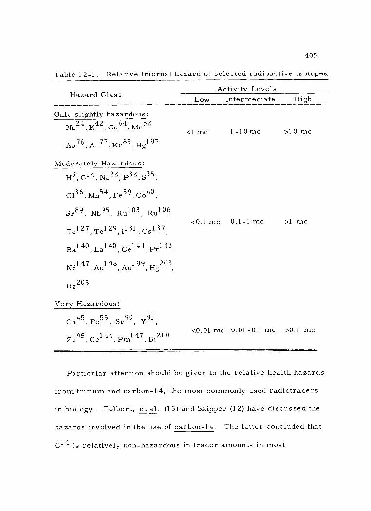
405
Table 1 2-1 . Relative internal hazard of selected radioactive isotopes.
Hazard Class Activity Levels
Low Intermediate High
Only slightly hazardous:
Na24, K42, Cu64, Mn52
As76, As77, Kr85, Hgl 97
Moderately Hazardous:
H3, C14, Na22, P32, S35,
C136, Mn54, Fe59, Co60,
Ru103 Rul06 Sr89, 89, Nb95,
Tel 27, Tel 29,11 31 Cs137
Bal 40, La140 Ce141 Pr143
Nd147 Aul 98 Aul 99, Hg203
Hg205
Very Hazardous:
Ca45, Fe55, Sr90, Y91,
Zr95, Ce144 Pml 47 Bi21 0
<1 mc 1 -1 0 mc >1 0 mc
<0.1 mc 0.1 -1 mc >1 mc
<0.01 mc 0.01 -0.1 mc >0.1 mc
Particular attention should be given to the relative health hazards
from tritium and carbon-1 4, the most commonly used radiotracers
in biology. Tolbert, et al. (13) and Skipper (12) have discussed the
hazards involved in the use of carbon -14. The latter concluded that
C14 is relatively non -hazardous in tracer amounts in most
406
experiments Inhaled CI 40 and ingested HC140 are rapidly ex-
2 3
creted, while inhaled particulate BaC14O3 undergoes 95 percent
turnover in about two hours. However, thymidine -C14 has a long
biological half -life, becoming incorporated into nucleic acids.
Handloser (6, p. 201 -202) has considered the health hazards in work-
ing with tritium. Tritium gas is less toxic than tritiated water. The
latter is readily absorbed by the skin by a factor of 1 04 greater than
tritium gas, thus requiring the wearing of gloves when handling it.
The maximum permissible body burdens and maximum per-
missible concentrations of radioisotopes in air and water for occupa-
tional exposure have been clearly stated (14, 21). For example, the
maximum permissible concentration of soluble C14 1 4 in water is 0. 02
µc /ml and of soluble tritium in water is 0.1 µc /ml. Maximum per-
missible body burdens of the two isotopes are 400 µc and 2, 000 µc,
respectively. By contrast the maximum permissible body burden
for a severely radiotoxic isotope such as Sr90 is only 204c, and that
for Pu239 is a mere 0. 4 µc.
Possible hazard from the use of tracer quantities of radio-
active isotopes is minimized by the maintenance of good laboratory
housekeeping and adherence to simple laboratory precautions as em-
bodied in the radiation laboratory rules set forth at the end of this
chapter. It will be seen that the fundamental purpose of these
407
safety rules is to prevent ingestion, inhalation or other entrance of
radioisotopes into the body and to reduce the amounts of external
irradiation to permissible levels. In general, it is a good principle
to treat all radioactive materials as if they were pathogenic bacteria,
even though they are being handled by purely chemical techniques.
Thus, the possibility of unnoticed contamination of the laboratory
or one's person should always be considered. However, in many
tracer experiments chemical and fire hazards will be far more signi-
ficant than any hazard from the radiation involved.
C. Radiation Monitoring Instrumentation
In order to determine the extent of possible radiation hazard
and /or detect contamination, radiation monitoring instruments must
be used. Although the institutional radiation safety officer may con-
duct periodic radiation surveys in tracer laboratories, it is basically
the responsibility of the individual isotope user to monitor his own
laboratory for radiation hazards. In addition, where millicurie
levels of gamma emitters are being used, each worker should have
proper personnel monitoring equipment. Among the many references
that might be cited in the field of radiological monitoring, perhaps
the National Bureau of Standards Handbook 51 (1 8) and the volume
by Handloser (5) would be the most suitable for radiotracer users.

408
1. Area monitoring
Area monitoring of laboratory facilities is normally carried
out by means of portable survey meters, although fixed monitors
are used in certain cases. The commonest portable monitor is a
battery operated G -M counter (see Chapter 4) with a ratemeter. It
is a very sensitive detector for relatively low levels of radiation,
either from shielded isotopic sources or contamination. G -M survey
meters are best used for the detection of radiation, not the measure-
ment of radiation dose -rate. However, if a G -M counter is calibrated
for a particular gamma energy, it can be used to measure the dose -
rate associated with that gamma energy. In general, readings in
cpm will be more meaningful than in mr /hr.
A second type of survey meter is a portable ionization cham-
ber (see Chapter 4) utilizing a vacuum -tube electrometer. Ionization
chamber survey meters are reliable, hold their calibration well, and
are relatively energy -independent. Their major use is for measure-
ment of gamma or x -ray dose -rate at moderate to high radiation
levels. They are commonly calibrated to read directly in mr /hr.
A variety of specialized area monitors are available. These
include such instruments as portable scintillation counters designed
either for alpha or gamma measurement, and air monitors (as for

409
tritium) that pull a volume of air over an ion chamber by means of
an air pump or fan.
2. Personnel monitoring
It is required by Atomic Energy Commission regulations (14,
part 20. 202) that those who enter areas where they are likely to re-
ceive a radiation exposure in excess of 25 percent of the maximum
permissible exposure must use appropriate personnel monitoring
equipment. A variety of such equipment is commercially available.
The film badge (8) is one of the most widely used personnel monitor-
ing devices, since the developed film serves as a permanent record
of the individual's cumulative exposure over a defined period, and
thus has some legal value. It usually consists of one or more film
packets in a compact plastic or metal container and is worn on the
clothing. Films with differential sensitivities to various radiation
types are available. The major disadvantage of the film badge is the
time lag between exposure and the evaluation of the developed film.
Films are changed and developed at regular intervals of one to two
weeks. In no cases, should the interval exceed a month. Film
badges are not required in many radiotracer experiments due to the
low activity levels in use or the character of the radiation exposure.
Pocket ionization chambers (about the size of a fountain pen)

41 0
are designed to be worn by the individual. These give a rough esti-
mate of the total exposure over the period from time of charging to
time of reading. In the form of dosimeters (electroscopes) the ac-
cumulated exposures may be read directly by the wearer at any
time, while pocket ionization chambers of a condenser type require
a separate reading instrument to determine the exposure.
D. Decontamination
The use of rubber or disposable polyethylene gloves and pro-
tective laboratory coats will usually eliminate the necessity for ri-
gorous skin decontamination. Likewise, if all handling of open ra-
dioisotopic sources is restricted to areas over trays (preferably
polished stainless steel) that are lined with absorbent paper, labora-
tory work surface contamination can be kept to a minimum. How-
ever, accidental contamination will generally occur on some occa-
sions despite the strictest precautions. A regular habit of monitor-
ing the hands and all working surfaces at the end of each working
period must be established to detect contamination. It should be re-
called again that the hazard from tracer doses of isotopic material
is primarily technical contamination of the laboratory, rather than
a threat to the health of the radioisotope user. National Bureau of
Standards Handbook 48 (1 6) will serve as a source of information on
411
the control and removal of radioactive contamination in laboratories.
Only general decontamination principles will be considered in this
chapter.
Routine hand washing for 2 -3 minutes with mild soap and
lukewarm water should always follow any handling of isotopic mate-
rial. After rinsing, the hands should be monitored. If this fails to
reduce contamination to an acceptable level, a repeated washing
using a soft brush and heavy lather may be required. Care must be
taken not to scratch or abrade the skin with the brush.
Laboratory clothing should be routinely monitored when high
levels of activity and /or more hazardous classes of isotopes are in
use. Contaminated garments should be washed in the laboratory be-
fore being released. Rubber gloves are usually decontaminated
readily by simple washing. Leather goods cannot be readily decon-
taminated.
Laboratory glassware and implements that have become con-
taminated must be thoroughly washed both to eliminate the radiation
hazard and the possibility of cross -contamination of successive ex-
periments. There is a considerable tendency for the adsorption of
radioactive materials onto glass. To reduce this problem, radio-
active solutions should never be allowed to dry on glass surfaces.
There is a considerable difference in the ease of
41 2
decontamination of various laboratory surface materials (10). Wood,
concrete, and soapstone are particularly difficult to decontaminate
due to their high porosity. This point will be more thoroughly dis-
cussed in Chapter 13. Polished stainless steel, vinyl floor coverings
and strippable plastic coatings are generally the materials of choice
with regard to ease of decontamination.
The routine cleaning of a radiotracer laboratory must take
into consideration the possibility of spreading contamination to other
areas. Depending on the activity level and hazard rating of the iso-
topes used, it may be necessary to restrict the cleaning implements
used to a single laboratory. Vacuum cleaners equipped with efficient
filters have been found particularly useful (7).
E. Radioactive Waste Disposal
Laboratory use of radioisotopes inevitably results in radio-
active wastes (i. e. , paper wipes, disposable implements, carcas-
ses, excreta, etc. ) that must be disposed of without endangering the
general public. Possible routes of disposal are into sewers, by in-
cineration, by venting directly into the atmosphere, by ground buri-
al, or by disposal at sea. Hopefully, the means of disposal required
will be reasonably convenient and economical.
Two general policies are usually followed in waste disposal.
41 3
In one, maximum dilution of the waste is sought, while in the other
maximum concentration is obtained. Disposal by dilution usually in-
volves release into the sewer, direct release into the air, or incine-
ration of the wastes. Atomic Energy Commission regulations (1 4,
part 20. 303) restrict disposal via sewage to material that is readily
soluble or dispersible in water and to activities below specified levels
(for example 100 µc of P32 per day). National Bureau of Standards
Handbook 49 (1 7) discusses in detail such disposal of P32 and 113 1
wastes. For many radiotracer applications this method offers both
convenience and safety. However, there is always the possibility
that some aquatic organisms (see Experiment E) may reconcentrate
these wastes to hazardous levels.
Direct release into the air via hood exhausts is feasible for
14 C 02 and other volatile or gaseous substances. However, dilution
by the air flow through the exhaust stack must be such that maximum
permissible concentrations are not exceeded (for example, for C 14
this concentration is 1 x 10 6 p.c/m1 air). Specific approval by the
Atomic Energy Commission is now required to dispose of radioactive
wastes by incineration (14, part 20. 305), previous published state-
ments notwithstanding.
Concentration and storage of radioactive wastes may be ne-
cessary for materials which cannot be disposed of by dilution.
414
However, this method is more suitable for high levels of activity,
such as reactor wastes (1). The storage may take the form of burial
in the soil or in concrete filled drums at sea. Soil burial is a parti-
cularly attractive method for disposing of carcasses and excreta
contaminated with isotopes that are non - combustible (for example,
iron, calcium, etc. ). The quantity of wastes and conditions of burial
have been clearly specified (14, part 20. 304). In a sense, burial
amounts to a type of dilution, since before the waste substances
enter the biosphere affecting man they will have hopefully been di-
luted below the hazardous level.
The physical half -life of the isotopic material in the waste
is an important determining factor as to the most satisfactory me-
thod of disposal, especially for insoluble materials. For tracer
levels of isotopes with half -lives of days to a few weeks, merely
holding the wastes in storage will reduce the activity to tolerable
levels. It can easily be calculated that after ten half -lives the ori-
ginal activity of a radioactive sample will be reduced by a factor of
1 , 000. Carcasses containing short -lived isotopic material can be
either preserved in formalin or frozen for such a term of storage.
The biologist is perhaps most concerned with C1 4 waste
disposal. Here, the long half -life precludes storage during decay.
National Bureau of Standards Handbook 53 (19) describes various
415
recommended methods of C14 waste disposal. One method that has
general application, but is often used for C14 is isotopic dilution.
Carbon -1 4 may be disposed of in any manner provided it is intimately
mixed with stable carbon, in the same chemical form, in a ratio
that never exceeds I pc of C14 for every 10 g or stable carbon. An
additional handbook (20) describes precautions in handling bodies
containing isotopes. Although this discussion concerns human
bodies, the principles apply to animal carcasses as well.
F. Radiotracer Laboratory Safety Rules
It is not feasible to set forth working rules that apply in all
situations. As has been seen, the activity level and hazard class of
the isotope being used will determine the degree of precaution re-
quired. However, the following list of regulations are intended to
minimize internal and external hazards, prevent technical contamina-
tion of the laboratory, and specifically comply with Atomic Energy
Commission rules (1 4).
1. Eating, storing, or the preparation of food, smoking, or
the application of cosmetics is forbidden in any area where radio-
active materials are stored or used.
2. Direct contact with radioactive materials must be avoided
by the use of protective laboratory coats, the wearing of rubber or
disposable plastic gloves, and the use of safety pipetters.

416
3. All spills of radioactive material must be reported to the
instructor or supervisor and decontaminated immediately.
4. Complete records of receipts, transfers and disposal of
radioactive materials must be kept.
5. A film badge should be worn whenever working with gam-
ma emitters at levels exceeding 1 00 µc.
6. Work should be carried out under a hood in all cases
where radioactive material may be lost by volatilization, dispersion
of dust, or by spraying or spattering. Wherever possible, work
with closed containers.
7. All radioactive samples should be properly labeled with
the isotope and activity, and covered.
8. Liquid wastes should not be poured into the drain or con-
taminated apparatus washed in the sink unless the levels of activity
entering the sewer system have been calculated as permissible (1 4,
part 20. 303).
9. The disposal of solid wastes and contaminated articles
(corks, paper wipes, etc. ) should be into designated containers,
and, under no consideration, into ordinary trash receptacles.
10.. The storage of all radioactive material must be in properly
designated locations.
417
11. At the close of a working period the laboratory work sur-
faces should be carefully monitored.
1 2. Before leaving the laboratory after working with active
materials, each person should wash his hands thoroughly and check
them with a monitoring instrument.
13. All laboratory glassware and equipment should be pro-
perly decontaminated after use before being returned to general
usage.
14. It is desirable to completely decontaminate one's hands
and work surfaces, but the following arbitrary surface contamination
tolerances (as measured by a G -M survey meter with a thin end-
window) may be allowed after efforts at decontamination:
Hands 350 cpm
Working surface 250 cpm
The arbitrary nature of any such tolerances should be recognized,
while on the other hand absolutely complete decontamination is not
always feasible.
BIBLIOGRAPHY
1. Amphlett, C. B. Treatment and disposal of radioactive wastes. New York, Pergamon Press, 1961. 289 p.
2. Andrews, Howard L. Radiation biophysics. Englewood Cliffs, N. J. , Prentice -Hall, 1 961. 328 p.
418
3. Blatz, Hanson (ed. ). Radiation hygiene handbook. New York, McGraw -Hill, 1 959. 926 p.
4. Catch, J. R. Radio -isotopes as tracers -- the rational approach. Research 9:479 -484. 1 956.
5. Handloser, John S. Health physics instrumentation. New York, Pergamon Press, 1959. 182 p.
6. . Tritium health physics considerations. In: S. Rothchild's advances in tracer methodology. vol. 1. New York, Plenum Press, 1 963. p. 201 -202.
7. Holden, F. R. , R. K. Skow and J. Todd. Vacuum cleaner for radioactive decontamination. Nucleonics 11(2):67. 1 953.
8. Jetter, Evelyn S. and Hanson Blatz. Film measurement of beta radiation dose. Nucleonics 10(10) :43 -45. 1952.
9. Kinsman, Simon (ed. ). Radiological health handbook. Rev. ed. Washington, U. S. Public Health Service, Division of Radio- logical Health, 1960. 468 p.
10. Lane, W. , et al. Contamination and decontamination of labora- tory bench -top materials. Nucleonics 11(8):49. 1 953.
11. National Academy of Sciences. The biological effects of atomic radiation. Summary reports. Washington, 1 956. 108 p.
1 2. Skipper, Howard E. The hazard involved in the use of carbon - 1 4. Nucleonics 1 0(2):40 -44. 1 952.
13. Tolbert, B. M. , N. Garden and P. T. Adams. Special equip- ment for C1 4 work. Nucleonics 11(3):56-58. 1 953.
14. U. S. Code of Federal Regulations (1 960), Title 10 -- Atomic energy, Part 20 -- Standards for protection against radia- tion.
15. U. S. Dept. of Commerce, National Bureau of Standards. Safe handling of radioactive isotopes. Washington, 1949. 30 p. (Handbook no. 42. )
419
1 6. . Control and removal of radioactive con- tamination in laboratories. Washington, 1951. 24 p. (Handbook no. 48. )
17. . Recommendations for waste disposal of phosphorus -32 and iodine -131 for medical users. Washing- ton, 1 951. 11 p. (Handbook no. 49. )
1 8. . Radiological monitoring methods and instruments. Washington, 1 952. 33 p. (Handbook no. 51. )
1 9. Recommendations for the disposal of carbon -14 wastes. Washington, 1953. 14 p. (Handbook no. 53. )
20. . Safe handling of bodies containing radio- active isotopes. Washington, 1958. 20 p. (Handbook no. 65. )
21. . Maximum permissible body burdens and maximum permissible concentrations of radionuclides in air and water for occupational exposure. Washington, 1 959. 95 p. (Handbook no. 69. )

CHAPTER 13 - DESIGN OF RADIOTRACER LABORATORIES
A. The Need for Specially Designed Laboratories
420
Recent advances in the use of radioisotopes as a research
tool have considerably broadened the scope of the field and have
created the need for specially designed laboratories to handle more
hazardous operations. This is true since, whereas low level experi-
ments can be and are being carried out in conventional laboratories,
these laboratories are generally inadequate to accommodate opera-
tions involving higher levels of radioactivity. Notable examples in
this regard are use of the Wilzbach method in the preparation of
tritium labeled compounds which often involves the use of multiple
curies of tritium gas; use of radioisotopes in studies with large
animals which often encounters problems in waste control; use of
biosynthetic methods to prepare carbon -14 labeled compounds having
a high specific activity which may involve tens of hundreds of milli -
curies of carbon -14; and use of gamma emitters at the multiple -
millicurie levels.
Laboratory facilities specially designed for these operations
are generally expensive with respect to both construction and asso-
ciated instrumentation. Consequently, it is often advisable to esta-
blish a coordinated laboratory in a scientific community to handle
421
hazardous radioisotope experiments for all research workers in the
area. Such a laboratory is designed to fulfill the following specific
functions:
(1) Housing and managing special facilities for the handling
of radioisotopes with respect to hazard control and waste
(2)
disposal control. Facilities are designed to handle experi-
ments involving "medium levels" of radioactivity (up to
ten millicuries of gamma or high energy beta emitters
and up to 100 millicuries of soft beta emitters) and "high
levels" of radioactivity (up to 100 millicuries of gamma
or high energy beta emitters up to one curie of C14 and
up to 100 curies of H3). 2
Housing and management of expensive instruments or
equipment that are not readily available to individual re-
search groups.
(3) Coordinated storage of radioisotopes and radioisotope
labeled compounds so that a continuous supply of short
half -life radioisotopes can be maintained and a faster
turnover of labeled compounds can be effected to avoid
undue radiolysis.
(4) Provision of a testing ground with professional consulta-
tion to enable research workers to evaluate the feasibility
422
of exploratory experiments.
B. The Planning Committee
In designing such a laboratory, in addition to ordinary consi-
derations necessary for the design of a science laboratory, attention
is also directed to unique features derived from the type of the ra-
dioisotope experiments that are to be carried out in the facility. It
is important that a planning committee be organized consisting of
scientists in a broad spectrum of disciplines, each familiar with the
use of radioisotopes. The chairman of such a committee serving
as a spokesman for the committee, should take the trouble to learn
some basic concepts in architecture and construction engineering so
that the committee's conclusions can be properly transmitted to the
architect and the administrative representative of the scientific
community. This can be accomplished by perusal of key references
in the literature. Especially valuable is the chapter by Ward (13)
and a recent symposium report on construction of laboratory build-
ings (2).
It is from the planning committee that issues such as: floor
space required, orientation of varied functions, type of laboratories,
special facilities to be housed; special instruments to be housed,
etc. , are determined. Decisions on these issues in turn determine

423
the construction budget. It should be recognized that the unit cost
per square foot for a laboratory of this type is slightly higher than
an ordinary science building, particularly in the area of mechanical
installation in view of the necessary elaborate ventilation and sewage
systems and radioisotope storage.
It is important that the architect assigned for the project be
one who possesses extensive experience in the design of science
buildings. To insure mutual understanding of the design task among
user, architect and administration representative (e. g. , the institu-
tional representative for construction), it is highly advisable that a
tour be taken by these three men to visit a number of existing radio-
isotope laboratories in the country. Such a visit will enable the
team to take advantage of unique good features of the existing instal-
lations and to avoid unnecessary and costly design mistakes.
C. Basic Design Prerequisites
Insofar as the basic design prerequisites are concerned,
they are primarily the same as those for conventional science build-
ings except for a few additional features. The selection of the build-
ing site should not only fulfill the requirements prevailing in the
scientific community, but should also take into consideration such
facets as: (1) hazard evaluation with respect to potential radioisotope

424
contents in air and in sewage water; (2) nature of projected programs
(Thus, if a research reactor is to be added as an annex to the build-
ing in the future to fulfill such functions as radioisotope production,
neutron activation analysis, etc. , it will be necessary to consult with
the Atomic Energy Commission in the selection of a proper site);
(3) soil loading requirement, which is of paramount importance to
the construction of a hot cell and other heavy shieldings; (4) relation
to supporting facilities elsewhere in the scientific community (The
facilities in the radioisotope laboratory are likely to be specialized
and the research capability of the workers in the building will be
greatly enhanced if supporting facilities are in nearby areas); (5)
plans for future expansion; (6) operational costs.
Due consideration should be given to selection of suitable
materials for construction, bearing in mind the necessity for a fire-
proof structure, shielding problems, and surface contamination pro-
blems. In deciding the type of building, one must recognize such
problems as: (1) size limitations with respect to necessary clear-
ance for equipment (i. e. , lifting devices, shielding devices, instru-
ments, etc. ); (2) the movement of rack - mounted instruments and
equipment inside the building; (3) the problems of radioisotope stor-
age; (4) compliance with existing regulations and building codes.
425
D. Specific Design Features
There are a number of specific design concepts unique to the
design of a radioisotope laboratory. Some of the important ones
will be discussed in the remainder of this chapter.
1. Floor arrangement
The arrangement of individual laboratories should be derived
from the following considerations:
(1) Segregation of areas on the basis of prevailing radiation
level. A logical arrangement calls for the zoning of
offices, counting rooms, animal quarter, low level lab-
oratories, high level laboratories, radioisotope storage,
and radioactive waste disposal. For the convenience of
the research workers, some of the laboratories can be
used as combination offices and laboratories.
(2) Utilities to laboratories can be best accommodated by
the insertion of a utility shaft between two rows of labor-
atories.
(3) Space clearances with respect to size of corridors,
doors, etc. , for the moving of instruments and equip-
ment.

426
(4) Control of access so that the building as a whole can be
considered as a restricted area.
(5) Ample space for storage to facilitate the good housekeep-
ing necessary in a radioisotope laboratory.
(6) Segregated solvent storage room to facilitate the control
of fire hazards.
(7) The use of airlock systems to control air contamination.
This is important in the event the ventilation system is
rendered inoperative during a power failure.
2. Ventilation and heating
The type of heating system for a radioisotope laboratory
should be one that facilitates good housekeeping. The system is
naturally related to the ventilation system designed for the building.
The most desirable design for the ventilation system in a radioiso-
tope laboratory calls for the unidirectional flow of air from the office
area to individual radioisotope laboratories, followed by exclusive
exhaust via radiochemical hoods equipped with absolute filters.
Recirculation of air can be permitted in the counting or instrument
rooms provided these rooms are pressurized against the corridors
to prevent contamination from the atmosphere in the corridor. Air
supply to individual laboratories is best provided from the corridor
427
via louvered doors or louvered walls.
It is preferred that no more than two rooms are serviced by
one exhaust blower so that ventilation control can be maintained in
event of localized mechanical failures. Housing the exhaust system,
including filter assembly for the hoods, in the utility shaft offers the
advantage of simplicity of the duct design and of accessibility to the
filters and exhaust system for routine maintenance. Stainless steel
is the preferred material for construction of ducts. However, other
materials such as fiberglas, are equally good. In a typical labora-
tory, having a total floor space of 400 sq. ft. and equipped with two
hoods, the total air displacement in the room should exceed 1,300
cubic feet per minute to provide adequate rates of air change in the
room. Several portable duct connections should be provided in each
room to permit the connection of such devices as glove boxes, respi-
ration chambers, etc. , to the exhaust.
3. Electrical utilities
The basic requirements of electrical utilities in a radioiso-
tope laboratory are similar to those for the ordinary chemistry or
physics laboratories. However, attention should be given to several
requirements unique to radioisotope laboratories. The extensive
instrumentation in handling and measurement of radioisotopes calls

428
for an ample supply of 120 volt a -c outlets. This can be provided by
wall outlets and particularly the outlets attached to drop -down cords
from the ceiling to allow maximum flexibility. The provision of 3-
phase 240 volt power outlets is equally important in accommodating
heavy equipment.
In a typical instrument room or counting room, it is highly
advisable to equip the power supply with a voltage stabilizer and to
isolate individual circuits so that cross interference of electronic
instruments can be avoided. Provisions in the nature of blank con-
duits should be made to accommodate present and future radiation
monitoring devices. An intercommunications system actuated by voice
or foot control is of some importance in the high level laboratories.
Selection of suitable lighting should bear in mind the ease
of housekeeping and the undesirable interference of fluorescent light
with liquid scintillation counting. Battery -powered emergency lights
are necessary provisions for inside rooms that rely extensively on
artificial lighting. Fire detection systems should be installed in
each of the laboratories with signals transmitted directly to the fire
station so that extensive fire damage can be avoided. Needless to
say, the solvent storage room should be equipped with an automatic
fire extinguishing system. Whenever possible, extra blank conduits
should be provided, particularly in the shielded area to permit

429
ready accommodation of future projects.
4. Sewage disposal
Several important facets should be considered in designing
the sewage system in a radioisotope laboratory. It is advisable to
segregate sewage systems under the categories of storm water,
toilet disposal, low level radioactive waste, and high level radioac-
tive waste. Whenever possible, it is preferable to dispose of liquid
radioactive waste of higher levels in isolated containers. The high
level sewage disposal system is primarily installed to handle area
contamination that cannot be readily controlled. This includes acci-
dental spills and more importantly, radioisotope studies with large
animals.
A retention system (one or more tanks 5, 000 gallons in
capacity) may be installed to permit temporary holding of radioactive
waste in the high level sewage system. Contents in the retention
tank can be either transferred to a waste liquid transporting truck
for permanent disposal, or allowed to decay in the case of short
half -life isotopes.
The low level sewage disposal system is designated to accom-
modate laboratory waste water from low level radioisotope labora-
tories. Since the waste is discharged directly into the public
430
sewage, an upper limit of radioactivity that can be disposed in each
laboratory over a given period should be defined. To insure absolute
control of hazards, it is advisable to install a liquid monitoring sys-
tem at the downstream end of the low level sewage line and provisions
should be made to connect the low level sewage line to the retention
tank in event of a major accidental spill. Most of the commercially
available liquid monitors are those capable of detecting gamma or
high energy beta emitters. It may be desirable to install a liquid
scintillation monitor in case tritium is used extensively in the labora-
tory.
Glass appears to be the most desirable material for sewage
piping because it is resistant to chemicals and allows ready visuali-
zation of stoppage in drains. It is important that the sewage line
should be exposed in the laboratory and in the utility shaft, as much
as possible to facilitate repair and replacement. The main sewage
line should be routed to the outside of the building as directly as pos-
sible to minimize length of concealed sections of the line.
Floor drains should be limited as much as possible. They
should be installed only in the areas where complete washdown of
rooms is essential to the operations. Even then, it may be desirable
to cap floor drains to minimize cross- contamination of rooms.
Master traps can be used to accommodate a number of sinks
431
and floor drains. Such an arrangement offers the advantage that the
lodging of radioactive materials in individual sink drains can be
avoided, whereas, cross contamination of areas through an untrapped
draining system can be prevented.
5. Radioactive waste disposal
Inasmuch as the basic principle underlying disposal of radio-
active waste calls for isolation or dilution, a waste disposal room
should be established as a separate unit in a radioisotops laboratory.
The room should be designed to store high levels of solid or liquid
radioactive waste prior to their transfer to a permanent disposal
site. It may also be desirable to install a commercial scale gar-
bage disposal unit so that low level solid wastes can be pulverized
and disposed of via the sewage system. It is also important to have
ample cold storage facilities to store radioactive biological speci-
mens such as animal carcasses. Adequate lifting devices should be
provided in this room to permit ready transfer of shielded waste to
exterior of the building. Incineration of low level waste containing
C14 or H3 is a convenient means of disposal, although the operation
is best carried out in remote areas.
432
6. Laboratory fixtures
The arrangement of laboratory fixtures in a radioisotope
laboratory should take into consideration ventilation requirement,
accessibility of utilities, and flexibility of room usage. Standardi-
zation of fixture arrangement in a modular sense is highly advisable
with respect to both program accommodations and economy in cost.
A typical arrangement in a modular radioisotope laboratory
for low level studies is given in Figure 13 -1 and an isometric view
of one half of the modular laboratory is shown in Figure 13 -2. Two
radiochemical hoods, ten inches apart, are housed along the middle
section of the wall next to the utility shaft. The location provides
one with the best air flow pattern. The ventilation system for this
room should be so designed that the air supply is provided from a
louvered door and the exhaust routed exclusively by way of the hoods.
Permanent benches with a sink are located alongside of each of the
hoods. Utilities to the permanent benches can be readily provided
from the utility shaft. The utilities to accommodate other portions
of the room are available, exposed on unistrut supports attached to
walls and floor. Such an arrangement makes available all utility
outlets, including cup sinks, on the utility shelf attached to the wall.
Equally important is the fact that utility accommodations of this type
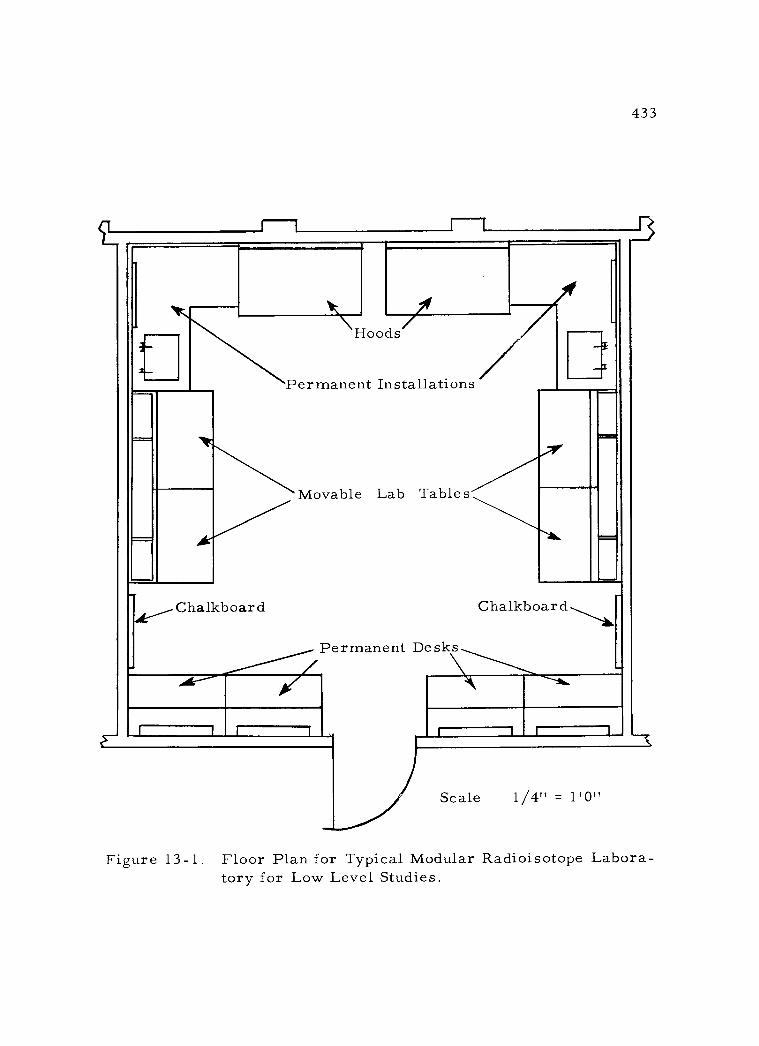
433
4-
Chalkboard
L--
\ /f H Hoods
Permanent Installations
Movable Lab Tables i Permanent Desks
f I I f
-4 -X
Chalkboard
Scale 1/4" = l'0"
Figure 13 -1, Floor Plan for Typical Modular Radioisotope Labora- tory for Low Level Studies.
y
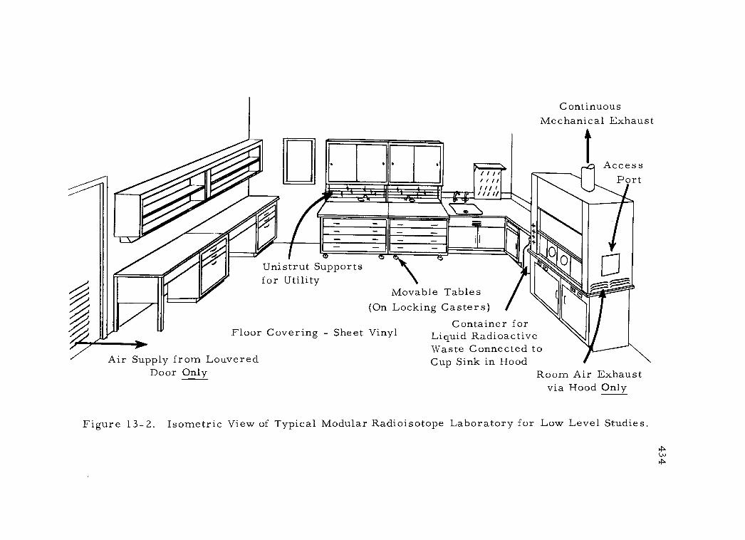
e ----; -- - . , vm._,-.a MMML[ ..
7;a1
Continuous Mechanical Exhaust
-c Access Port
Unistrut Supports for Utility
Movable Tables (On Locking Casters)
Container for Liquid Radioactive Waste Connected to Cup Sink in Hood
Floor Covering - Sheet Vinyl
Air Supply from Louvered Door Only Room Air Exhaust
via Hood Only
Figure 13 -2. Isometric View of Typical Modular Radioisotope Laboratory for Low Level Studies.
i
435
permit the use of movable benches.
In the depicted arrangement (Figure 13-1), four 4 -foot mov-
able benches are provided in the room. Each of the movable benches
is equipped with an electric strip outlet underneath the edge of the
bench top. The strip can be connected either to the wall outlet or
the ceiling drop -cord outlets. Maximum flexibility in room usage
is offered by this arrangement since in a radioisotope laboratory,
it is often desirable to have ample space next to a laboratory bench
to accommodate gas tanks, rack -mounted instruments and portable
vacuum benches. The movable benches can be used as single or
double wall benches or as an island bench.
Four desks are located on the side of the laboratory next to
the corridor. Each is equipped with electric strip outlets so that
they can be connected to a permanent outlet. The nature of the desk
provides dual usage, either as an office desk or as an instrument
table.
Steel is the preferred material for construction of laboratory
benches or instrument desks, primarily because of the ease of de-
contamination. Insofar as the bench top material is concerned, ex-
tensive tests on many types of available materials have led to the
designation of stainless steel as the best material because of its
excellent resistance to chemical agents and the ease with which it
436
is decontaminated in the event of minor spills. The laboratory floor
should be covered with sheet vinyl to facilitate decontamination oper-
ations.
One or more laboratories should be designed to accommodate
radioisotope work at higher levels. This is particularly important
if one desires to carry out Wilzbach operations for labeling of com-
pounds with tritium. It is preferred that the high level laboratory
be segregated from low level rooms by means of an air lock system
to permit better control of air contamination. In addition to regular
radiochemical hoods, the high level laboratory should be equipped
with awalk -in hood of sufficient size to accommodate a portable vac-
uum bench and pertinent laboratory equipment. Air movement in
this laboratory should be approximately 3, 000 cubic feet per minute
and all exhausts must pass through absolute filters. It is desirable
to extend the exhaust stack from the high level laboratory at least
ten feet above any nearby buildings. This will provide adequate air
dilution in the event of an accident involving the release of curie
amounts of tritium gas or other radioactive compounds that cannot
be removed by the filter. It is important to provide this laboratory
with an intercommunications system so that good contact with other
personnel in the area can be readily maintained.

437
7. Radiochemical hoods
A typical radiochemical hood which can be used for low or
high level radiochemical work is depicted in the plan of the modular
laboratory (Figure 13 -2). The hood must designed as a constant -
flow type since ventilation of the room relies exclusively on the con-
tinuous hood exhaust. When the front opening of the hood is closed,
the bypass sash should automatically open to allow the passage of a
constant amount of air through the hood. The hood is constructed of
steel with the inside wall lined with transite and bench tops covered
with stainless steel. Coating the transite walls with strippable paint
permits ready decontamination from time to time. Controls of all
utility outlets in the hood are mounted on one side of the front frame
with piping exposed. This will facilitate repair and replacement of
the utility system. Unique features of the radiochemical hood of this
type are:
(1) The front window can be readily replaced with a panel
equipped to accommodate a pair of gloves. This is es-
sential if one desires to have absolute prevention of air
contamination through back flow of the hood atmosphere,
in more hazardous operations.
(2) The hood is equipped with two cup sinks: one is of the
438
ordinary laboratory type, the other mounted flush with
the bench top, is specially designed to permit the trans-
fer of liquid radioactive waste directly into a carboy
stored underneath the adjacent bench.
(3) A small access port on one side of the hood wall (see
Figure 1 3-2) to permit direct transfer of solid radio-
active waste into a storage container housed in the space
between the two adjacent hoods (Figure 1 3-1).
The air movement through the depicted radiochemical hood
is 125 linear feet per minute across each front foot. Since the hood
is five feet in length, the total air flow through the hood is approxi-
mately 625 cubic feet per minute. The absolute filter for each of
the hoods is housed in the utility shaft with the blower housed in the
mechanical space in the ceiling of the shaft immediately before the
exhaust stack.
It should be emphasized that this chapter represents merely
an attempt to bring out important facets that must be considered in
the design of a radioisotope laboratory. No universal recommenda-
tions are intended inasmuch as it is impossible to set forth criteria
to suit individual tastes and individual purposes.

439
BIBLIOGRAPHY
1. Branson, Byron M. , et al. Assembly and operation of a low - level counting facility. Journal American Water Works Association 51 :438-448. 1 959.
2. Design and construction of laboratory buildings. Analytical Chemistry 34(1 0) :25A -46A. 1 962.
3. Design and construction of radiochemical laboratories. A se- lected list of unclassified references. 1 951. 5 p. (U. S. Atomic Energy Commission. TID- 3013).
4. Garden, Nelson B. Semihot laboratories. Industrial and Engi- neering Chemistry 41:237-238. 1 949.
5. Grinberg, B. and Y. LeGallic. Caractéristiques fondamentales d'un laboratoire de mesure de trés faibles activités. The International Journal of Applied Radiation and Isotopes 12:104 -117. 1961.
6. Levy, Henri A. Remodeling a laboratory for radiochemical instruction or research. Industrial and Engineering Chemis- try 41:248-250. 1949.
7. Mackintosh, A. D. The architectural approach to radiochemical laboratory design. 1 949. 31 p. (U. S. Atomic Energy Commission. AECU -210; ORN L -335)
8. Norris, William P. Radiobiochemical laboratories. Industrial and Engineering Chemistry 41 :231 -232. 1 949.
9. Rice, C. N. Laboratory for preparation and use of radioactive organic compounds. Industrial and Engineering Chemistry 41:244- 248. 1 949.
1 0. Swartout, J. A. Research with low levels of radioactivity. Industrial and Engineering Chemistry 41 :233 -236. 1949.
11. Tompkins, Paul C. A radioisotope building. Industrial and Engineering Chemistry 41 :239 -244. 1 949.
440
12. Tompkins, Paul C. and Henri A. Levy. Impact of radioactivity on chemical laboratory techniques and design. Industrial and Engineering Chemistry 41:228-231. 1949.
13. Ward, Donald R. Low level radioisotope laboratories. In: Laboratory planning for chemistry and chemical engineering. New York, Reinhold, 1962. p. 156 -170.
14. Webster, S. H. , E. J. Liljegren and C. C. Powell. Hood for radioactivity work. Nucleonics 10(4):65 -67. 1952.

PART TWO
BASIC EXPERIMENTS
IN THE
MEASUREMENT OF RADIOACTIVITY
441
EXPERIMENT I - OPERATION AND CHARACTERISTICS OF A GEIGER -MUELLER COUNTER
The nature and construction of Geiger - Mueller (G -M) detectors
has been extensively discussed in Chapter 4. It has been seen that they
are ionization chambers operated at a potential high enough to give the
maximum usable gas amplification for an ionizing event within them.
G -M tubes are perhaps the most widely used detectors for radioactivity
determinations because of their simplicity and utility. The following
experiment is designed to serve as an introduction to some of the com-
ponent functions and operating characteristics of an entire G -M count-
ing assembly.
A. Component Functions of a Geiger -Mueller Counter Assembly
1. Power supply
This unit provides the necessary d -c potential across the elec-
trodes of the G -M detector so that gas amplification through second-
ary ionization can be facilitated and the electrons formed therefrom
can be readily collected on the anode. The voltage provided ranges
from 500 - 5000 volts with different models, but 1 500 volts is normal-
ly sufficient to operate most G -M detectors. A high degree of stability
in the power supply is not necessary for G -M detectors since minor
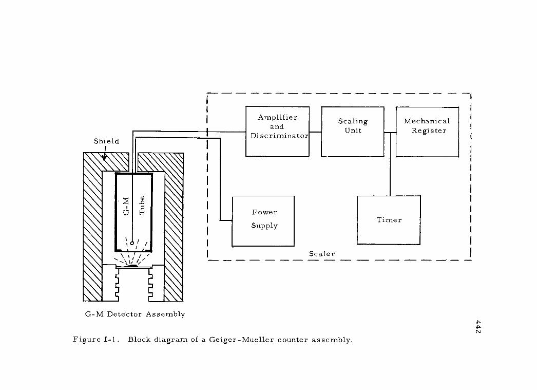
Shield
G -M Detector Assembly
Amplifier and
Discriminator
Power Supply
Scaling Unit
Scaler
Figure I-1. Block diagram of a Geiger - Mueller counter assembly.
Mechanical Register
Timer
443
voltage fluctuations do not bring about serious changes in the count
rate observed within the operating plateau. A high -voltage transfor-
mer, rectifier and voltage regulator comprise this component.
2. G -M detector assembly
The term detector is used to designate the G -M tube, whereas
counter applies to the entire counting assembly. The detector itself
is usually surrounded by a lead shield to reduce interference derived
from background radiation. In order to maintain a defined sample -
to- detector geometry, a rigid sample holding device, with several
shelves, is included in the assembly.
3. Amplifier and discriminator
Since the pulses from the G -M Detector are of moderate size
(several volts), extensive amplification is not required. Consequently,
a more important function of the amplifier is to shape the pulses into a
form more suitable for actuating the counting device. There is no
need for a high degree of linearity in the amplifier used in a G -M
counting assembly, since preservation of relative pulse height is not
necessary. Pulses of all sizes from the G -M detector after amplifi-
cation are passed to the discriminator, or trigger circuit. The dis-
criminator has two functions: (1) it establishes a pulse- height
444
threshold, permitting discrimination against noise pulses, and (2) it
produces a standardized pulse to actuate the scaling unit. Amplifier
and trigger circuits in past years have commonly utilized vacuum
tubes, which added considerably to the bulk of these components. Re-
cent use of transistorized circuits has allowed a very great reduction
in component volume.
4. Scaling unit
With a moderate amount of radioactivity in a given sample, the
pulse rate from a G -M detector will be too high to be handled by an
ordinary mechanical register. Consequently, scaling stages are in-
terposed to group the pulses prior to the actuation of the mechanical
register. Scaling can be done by means of scale -of -2 (binary) or
scale-of-10 (decade) circuits, which are commonly used in multiples.
As an example, two decade scales in a series would feed only one
pulse to the register for each 100 incoming pulses to the scaler. In
this case, the true number of pulses detected would be found by multi-
plying the register reading by 100 and adding the interpolation indi-
cated by the scaler lights. Most recent scalers eliminate the use of a
register at all by employing scaling units based on cold cathode de-
cades. These incorporate a scale -of -10 in one tube and can be used
in multiples of five or six for direct reading of the total count from a
445
sample. Since the resolving time of the G -M detector is rather long,
a rapidly responding ( "fast ") scaler is not as essential with it as it is
with proportional and scintillation detectors.
5. Mechanical register
As indicated above, the mechanical register displays some
multiple of the pulse count -- usually 64x, 256x, 100x, or 1000x.
Even if used in conjunction with circuits, this unit can be overwhelm-
ed when the pulse rate is exceedingly high, resulting in a significant
loss of counting events. Many commercially available G -M counters
include a presetting arrangement, by which the counting process will
be terminated when a preset count is reached.
6. Timer
The accurate timing of counting duration is essential. Most
commonly these timing units are operated by a synchronous motor
drive directly controlled by the frequency of the alternating current.
More elaborate models also include a presetting device, whereby the
counting process can be stopped after a pre- determined time.
7. G -M counting assembly
In the commercially available instruments, the power supply,

446
amplifier, discriminator, scaling units, register, and often the ti-
mer are commonly grouped together in a single housing, for which the
extended term "scaler" is used. This term is not to be confused with
the scaling circuits alone, which are only a part of the scaler. The
scaler, used in conjunction with a G -M detector in a lead shield and
sample support, constitutes a G -M counting assembly, or simply a
G -M counter.
B. Operation of a Geiger -Mueller Counter
1. General instructions
Although there are certain fundamental steps that apply to the
operation of all G -M counters, each model has distinctive individual
features. Consequently, the first step to be followed before operating
a given counter is to read through the manual of instructions furnished
by the manufacturer.
It will be recalled that G -M tubes can be permanently damaged
by the use of excessive d -c potentials (see Chapter 4). Always be cer-
tain that the high - voltage control is turned off, or as far down as pos-
sible, before turning on the scaler. This is a most important precau-
tion to be observed when operating the G -M counter.
The sample holder under the G -M tube usually has several

447
shelf positions on which the radioactive samples may be placed for
counting. These shelf positions, therefore, define the geometry of
sample -to- detector, which is essential in obtaining reproducible and
comparable results. Caution should be excercised to avoid the con-
tact of the counting sample with the detector window, both because the
window may become contaminated in this way, and because the thin
windows are extremely fragile.
2. G -M plateau and operating potential
In order to determine the effect of applied potential on the be-
havior of a G -M detector, insert a prepared radioactive sample (for
example C14 or Radium DEF into a defined geometrical position in
the sample support. A few minutes after the counter circuits have
been turned on, move the "count" switch to "on" and slowly increase
the potential in the detector by adjusting the high voltage control.
When the potential reaches a certain level, pulses from the detector
begin to be registered in the scaling circuits. Record this potential
as the "starting potential" and collect 3, 000 to 5, 000 counts at this set-
ting, noting the counting time. Repeat this procedure at successive
50 volt intervals. The count rate will rise rapidly, then level off when
the G -M plateau is reached. The plateau should extend approximately
300 volts followed by a sharp rise. Do not attempt to observe this

448
rise since at that stage continuous discharge occurs (see Chapter 4)
and the G -M detector can be permanently damaged.
Prepare a table indicating (1) potential applied to tube, (2)
total number of counts, (3) counting time, and (4) computed counts per
minute (cpm). From this information plot a graph with counts per
minute as the ordinate and tube voltage as abscissa (see Chapter 4).
The optimal operating voltage is usually chosen as 75 -100 volts above
the beginning, or threshold, of the plateau. Continued use of higher
potentials may shorten the detector tube life somewhat. An operating
voltage for each G -M tube is generally recommended by the manufac-
turer. How does your determined value compare with the manufac-
turer's? As G -M tubes age the plateau becomes altered. For this
reason the slope of the plateau should be checked at regular intervals
by a new determination of the plateau. When the slope of the plateau
varies more than 20 percent over a 100 volt span, the detector should
be replaced.
3. Background
The background radiation level should now be determined with
the G -M tube at the correct operating voltage. A counting duration of
at least ten minutes should be used. It should be realized that the stan-
dard deviation for a count rate determination decreases with the
449
number of counts accumulated (see Chapter 9). With low background
counting rates, it is not feasible, during the limited laboratory period,
to collect sufficient counts so that the relative standard deviation of
the background matches that associated with the counting of a radio-
active sample. However, in true determinations the counting time of
the background must be determined on the same statistical basis as
used for the sample.
While much of the background radiation comes inescapably
from natural radioactive materials and cosmic ray effects, radioactive
contamination of a laboratory or inadvertent placement of radioactive
samples in the vicinity of the counter can and should be scrupulously
avoided.
Background determinations should be made each time a group
of radioactive samples are to be counted, or at least daily. The back-
ground count rate must then be subtracted from each sample count
rate to arrive at the count rate due to the sample alone. If an unusu-
ally high background is encountered on some occasion, its cause
should be sought immediately.
4. Counter resolving time -- coincidence loss
In Chapter 4 it was indicated that, following an ionization in-
cident in a G -M detector, an avalanche of electrons rushes to the

450
anode wire. This initiates a negative pulse in the scaler circuit. The
movement of positive ions to the cathode wall is much slower. During
the brief interval while these events are occurring the detector is
either unresponsive (dead time) or too weakly responsive to produce a
pulse exceeding the discriminator threshold (recovery time). This
total interval during which succeeding ionization events are not regis-
tered is known as the resolving time of the detector. At higher count
rates this factor may lead to an observed count rate considerably less
than the true rate. The difference between these two values is the
coincidence loss.
The resolving time of a G -M detector can be observed directly
by means of an oscilloscope. However, it can also be determined by
means of the "paired source method ". To this end, cut a flat metal
planchet into two equal halves. Number them at the outer edge #1 and
#2 respectively (see Figure I -2). Toward the center of the flat edge of
each, place roughly equal amounts of a suitable radioactive sample.
Aqueous solutions of NaH2P32O4 or Co60C12, or powdered U3Og are
suggested. Each should give a count rate of 7, 000 to 1 0, 000 cpm on
the top shelf of the sample support.
Insert the two sources into the appropriate shelf of the sample
support without any overlapping of the two halves. Now count the two
samples (m ) for one minute and record the result. Carefully 1,2
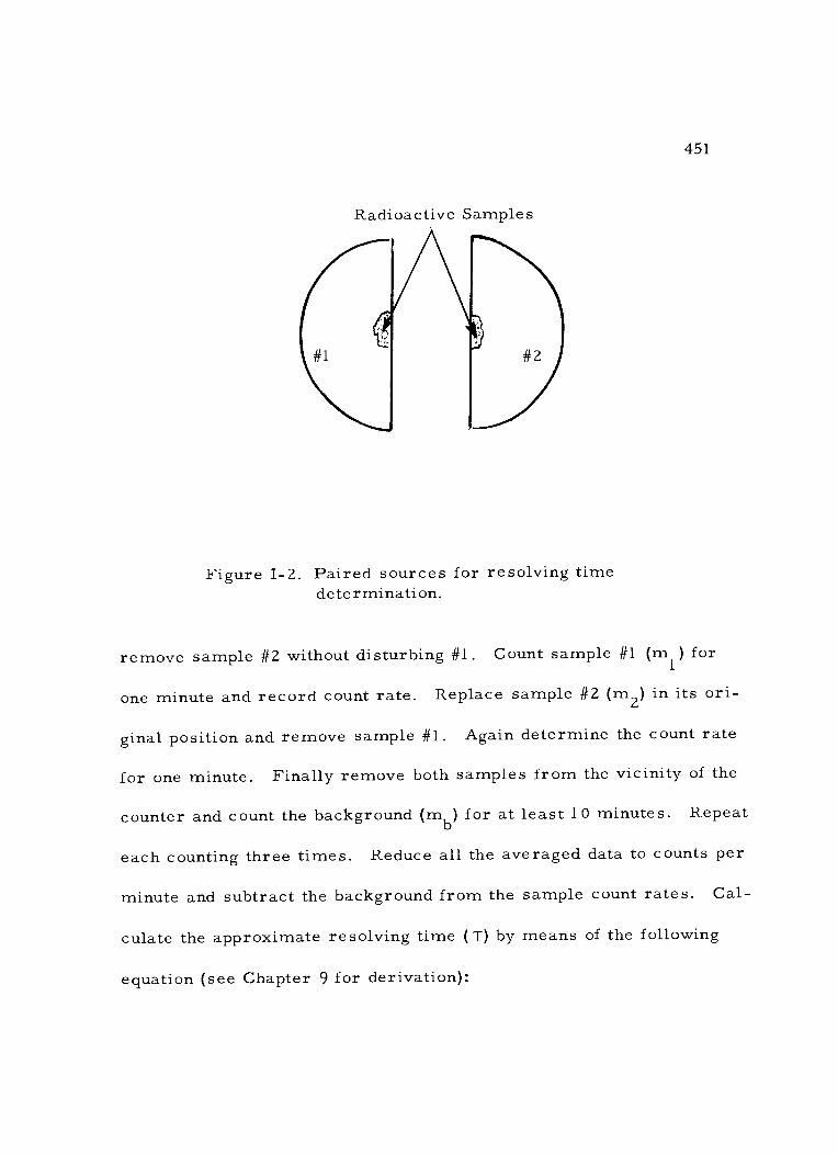
451
Radioactive Samples
Figure I -2. Paired sources for resolving time determination.
remove sample #2 without disturbing #1. Count sample #1 (m ) for 1
one minute and record count rate. Replace sample #2 (m2) in its ori-
ginal position and remove sample #1. Again determine the count rate
for one minute. Finally remove both samples from the vicinity of the
counter and count the background (mb) for at least 10 minutes. Repeat
each counting three times. Reduce all the averaged data to counts per
minute and subtract the background from the sample count rates. Cal-
culate the approximate resolving time (T) by means of the following
equation (see Chapter 9 for derivation):
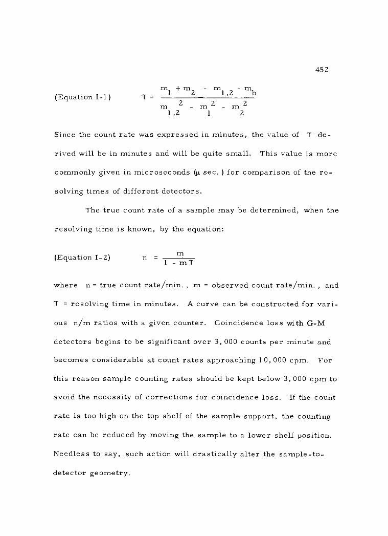
(Equation I-1) T- ml + m2 - ml ,2 - mb
m 2- m 2 - m 2 1,2 1 2
452
Since the count rate was expressed in minutes, the value of T de-
rived will be in minutes and will be quite small. This value is more
commonly given in microseconds (p. sec. ) for comparison of the re-
solving times of different detectors.
The true count rate of a sample may be determined, when the
resolving time is known, by the equation:
(Equation I-2) n - m 1 - mT
where n= true count rate /min. , m = observed count rate /min. , and
T = resolving time in minutes. A curve can be constructed for vari-
ous n/m ratios with a given counter. Coincidence loss with G -M
detectors begins to be significant over 3, 000 counts per minute and
becomes considerable at count rates approaching 1 0, 000 cpm. For
this reason sample counting rates should be kept below 3, 000 cpm to
avoid the necessity of corrections for coincidence loss. If the count
rate is too high on the top shelf of the sample support, the counting
rate can be reduced by moving the sample to a lower shelf position.
Needless to say, such action will drastically alter the sample -to-
detector geometry.

453
5. Shelf ratio and geometry
A radioactive sample can be centered under the G -M tube win-
dow by correct positioning on the sample support. However, its dis-
tance from the detector window will vary depending on which shelf is
used. Two or more such shelf positions are normally available in the
sample holder. Any comparison of count rates for samples counted on
different shelves must take into account the inverse square relation
between count rate and distance from the detector referred to in sec-
tion 4 above. For the purpose of such comparisons it is valuable to
find the ratio of count rates for the various shelves (shelf ratio).
Comparisons can only be made between samples of the same isotope
and under the same sample conditions.
Using the radioactive sample from section 2 above, determine
the net count rate on each of the shelves provided in the sample holder.
Then arbitrarily assign the top shelf position a value of 1. 0 and calcu-
late the shelf ratios for the other shelves by dividing the top shelf
count rate into each other value successively. This shelf ratio will
then indicate clearly the fraction of counts observed on the given shelf
compared to what would be observed on the top shelf position. It
should be noted that these values apply only to the isotope and detector
employed. A detector with a thicker window would, of course,
454
transmit less radiation. Likewise, an isotope emitting lower energy
radiation would suffer greater air absorption.
Summary:
In this experiment several important operational characteris-
tics of the G -M counter have been examined. To correctly operate
the counter, the position of the G -M plateau with respect to voltage
applied to the detector tube must first be found. The background radi-
ation level should always be determined and subtracted from the gross
sample count rate. The relatively long resolving time of the G -M
counter necessitates keeping count rates fairly low and /or making
corrections for coincidence loss. If shelf ratios are calculated, count
rates for samples of the same type counted on different shelf positions
may be compared.
455
EXPERIMENT II - OPERATION AND CHARACTERISTICS OF A PROPORTIONAL COUNTER
Various types of proportional detectors have been discussed in
Chapter 4. It will be recalled that they are ionization -type detectors
that are operated within a potential range where moderate gas amplifi-
cation occurs. A distinctive feature of this level of gas amplification
is that proportionality is maintained between the size of the output
pulse from the detector and the magnitude of the initial ionization with-
in it. The following experiment is designed to serve as an introduction
to some of the component functions and operating characteristics of an
entire proportional counter assembly.
A. Functions of the Components of a Proportional Counting Assembly
1. Power Supply
The d -c potential needed across the proportional chamber
electrodes to facilitate gas amplification varies widely with the
type of chamber and the composition and pressure of the counter
atmosphere. Normally a power supply that can be regulated up to
at least 2500 volts is adequate, but in some counting assemblies
5000 volts may be required. The voltage output must be reasonably
stable for porportional counting since the gas amplification factor
is heavily dependent on the potential gradient within the chamber.
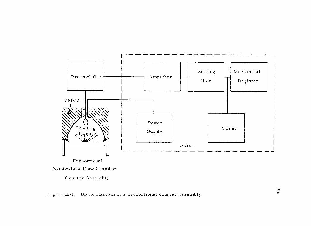
Preamplifier
Shield
Counting Chamber, NIL/ley
Proportional Windowless Flow Chamber
Counter Assembly
Amplifier
Power
Supply
Scaling
Unit
Scaler
Figure II-l. Block diagram of a proportional counter assembly.
Mechanical
Register
Timer
E
457
While G -M counters require a stability of power supply of only about
±1 the proportional counter requires better than ±0. 1 %.
2. Proportional detector assembly
Proportional detectors may be of various types. Its greater ef-
ficiency for detection of alpha or weak beta particles makes the window-
less flow chamber variety the most widely used in radiochemical analy-
sis. The following discussion pertains particularly to this type of de-
tector.
In the windowless flow counter, the radioactive sample is placed
inside the counting chamber and exposed to the counting atmosphere
directly without a window barrier intervening. The counting gas mix-
ture, usually methane or an argon- methane mixture, passes through the
chamber continuously during the counting operation. When a new sam-
ple is inserted, air that has been unavoidably introduced must be
"purged" from the chamber atmosphere by a brief increase in the flow
rate of the counting gas.
The counting chamber is commonly hemispherical in shape with
a thin anode loop suspended from the top. The chamber wall serves as
the cathode. The sample - holding planchet itself acts as the lower side
of the chamber. The planchet is introduced and held firmly in place by
means of a movable piston to give a defined geometrical relationship of

458
sample -to- chamber. The geometry of sample -to- chamber is close
to a solid angle of 2 n, which further increases detection efficiency.
Lead shielding is normally used to reduce the interference of back-
ground radiation.
3. Preamplifier
The output signal from a proportional detector will seldom
exceed 50m v. Thus, in situations where the pulses from the detec-
tor must pass to the scaler through cables of even a few feet in length,
a preamplifier is necessary. This is not usually the case where the
detector is an integral part of the scaler itself.
4. Amplifier
Since the gas amplification factor is considerably lower in the
proportional region than that in the Geiger region, a high gain ampli-
fier is usually required. This amplifier must be highly stable. In ad-
dition, the pulse sizes initiated by different ionizing particles vary
considerably. Consequeri ly this component must be able to amplify
a wide range of pulses linearly without distortion. By contrast, all
pulses from the G -M detector tube are of nearly equal size, so that
amplifier linearity is not so crucial there.
5. Scaling unit
459
What has been previously said concerning scaling units in G -M
counters applies here as well. Whereas the dead time of a G -M de-
tector is relatively long (up to several hundred microseconds), the
proportional detector generally has a very short dead time ( a few
microseconds). Consequently, a compatibly fast scaling unit is essen-
tial in order to take advantage of this feature.
6. Mechanical register and timer
These are usually no different from the same components des-
cribed for G -M counters in Experiment I.
B. Operation of the Proportional Counting Assembly
The instruction manual furnished with a particular counting
assembly should always be read thoroughly before operation of the
counter is attempted. For the windowless flow counter it is especially
important to become familiar with the technique of introducing a sam-
ple into the counting chamber and controlling the gas flow.
1. Proportional plateaus and optimal operating potentials
Make sure that the high voltage control is turned as low as
460
possible. Then turn the instrument "on" and wait at least five minutes
before proceeding. The input sensitivity, if adjustable, is usually set
quite low (at about 1 millivolt). This is in marked contrast to the sen-
sitivity normally used with G -M counters (0. 25 volts).
Insert into the counting chamber a prepared sample which
emits both alpha and beta particles. Often these are furnished with
the instrument. Otherwise a thorium or a uranium salt, or a radium
DE F preparation is suggested for this purpose.
Purge the counting chamber with the counting gas for about 1 -
2 minutes. Then reduce the gas flow to the continuous rate specified
by the manufacturer, usually one bubble per second through the bub-
bler.
Now slowly raise the potential across the detector electrodes to
the point where pulses begin to be registered (about 700 volts), and
collect at least 3, 000 to 5, 000 counts at this potential setting. If
counting does not begin at about the voltage specified, the chamber
may have been incompletely purged. Repeat this procedure at 50 volt
intervals up to the point at which the count -rate begins an abrupt rise
from the second (beta) plateau (usually about 2000 volts).
Record the results in tabular form and plot a graph of applied
potential vs. computed counts per minute (cpm). This should result
in a curve with two plateaus. The plateau at lower potential (alpha

461
plateau) reflects the counting rate of the alpha components of the sam-
ple, while that at the higher potential (beta plateau) includes both the
alpha and beta counting rates. See Chapter 4 (pages 147 -149) for de-
tails on this relationship.
The optimum operating voltages are usually determined as
the centers of the respective plateaus. Determine and record this
point for each plateau. Routine checks of this value should be made
with a suitable standard from time to time.
2. Differential counting of alpha vs. beta particles
Note that for mixed alpha -beta samples the pulses resulting
from beta particles cannot be directly counted apart from those re-
sulting from the alpha component. The count rate at the alpha plateau
can, however, be subtracted from the rate on the beta plateau to find
approximately the net beta count rate if desired. In addition, where
the beta particle energy is sufficiently high, a thin absorber placed
over the sample allows nearly all the beta particles to pass through,
while completely absorbing the alpha radiation. Alpha particles, on
the contrary, can be counted in the presence of beta -emission (and
gamma, too), by operating the detector at the alpha plateau. This
feature is one of the great advantages of the proportional counter over
the G -M counter. See the discussion of gas amplification in Chapter

4 for further explanation.
3. Counter resolving time
462
Paired radioactive samples such as those used to determine counter
resolving time with the G -M counter, but with count rates of 50, 000
to 1 00, 000 cpm each, should now be used for the same purpose with
the proportional counter. Operating on the beta -plateau, follow the
instructions given for the determination of resolving tine with the
G -M counter. Record data and calculate resolving time (T) using
Equation I -1. How do the resolving times of G -M and proportional
counters compare?
4. Background
An important additional feature of the proportional counter is
the magnitude of the background radiation level. On the alpha plateau
the background may be as low as 1 cpm, and comes almost entirely
from chamber contamination or natural radioactivity in the detector
materials. Why? On the beta plateau, the background may be about
50 cpm, and is mainly from external sources, as with the G -M count-
er. Determine the background rate for a reasonable period of time
(at least ten minutes) on each plateau and compare the results. With
a windowless detector there is a great hazard of contaminating the
463
counting chamber itself by fine dust or vapors from radioactive sam-
ples. It is important to check frequently the background level of a
windowless counter, whether it is of the G -M or proportional type.
Decontamination of the counting chamber will be necessary if the back-
ground level is permanently elevated.
C. Summary
Three salient operating characteristics of the proportional
counter have been explored in this experiment. The double plateau
(alpha and beta) allows the discrimination of particle type with a mixed
alpha -beta emitting sample. The much shorter resolving time makes
it possible to accommodate high counting rates (up to 100, 000 cpm)
without significant coincidence loss. Finally, the very low background
radiation level on the alpha plateau makes possible the counting of
very low activity alpha samples.

464
EXPERIMENT III - OPERATION AND CHARACTERISTICS OF AN EXTERNAL -SAMPLE (SOLID) SCINTILLATION COUNTER
The detection of an external source of radiation by means of
a scintillation crystal coupled to a photo -multiplier tube has been des-
cribed in Chapter 5. This method of detection differs sharply from
that of the ionization -type detectors (G -M, proportional, etc. ). It
depends on the interaction of radiation with a crystal fluor to emit a
number of photons proportional to the radiation energy dissipated.
These photons are converted to photoelectrons by the photocathode of
the adjacent photomultiplier, which are then greatly amplified through
a dynode chain to produce a pulse. As with the other counting assem-
blies, a scaler is attached to record the detector pulses. A wide
variety of external scintillation counting assemblies is at present
commercially available. The experiment that follows will introduce
the reader to a typical counting assembly.
A. Functions of the Components of an External Scintillation Counter Assembly
1. Power supply
The d -c potential supplied to the scintillation detector plays a
different role than it does in G -M and proportional detectors. Here
it is used to impress a stepwise increase of potential on the succes-
sive dynodes of the photomultiplier. Because this potential gradient
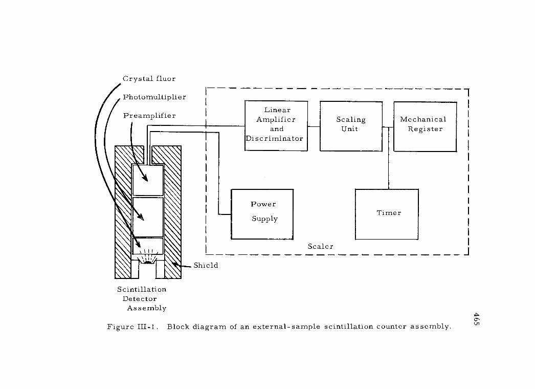
Crystal fluor
:::::::el. Linear Amplifier Scaling Mechanical
and Unit Register Discriminator
011 ¡;:i
Scintillation Detector Assembly
Shield
Power
Supply
Scaler
Timer
Figure III -1 . Block diagram of an external - sample scintillation counter assembly.
Preamplifier
-
/ /
J
466
in the photomultiplier so directly affects the degree of amplification
occurring, it is quite essential that the power supply by both highly
stable and well regulated. This point is particularly crucial if pulse
height analysis is to be attempted. It is usually sufficient to employ
a power supply with an output potential adjustable up to 3000 volts to
operate most photomultipliers.
2. Scintillation detector assembly
The lead shielding and sample support used are normally sim-
ilar to those found in G -M detector assemblies. However, due to the
greater efficiency of the scintillation process for detecting gamma
rays, and thus also the cosmic ray background radiation, lead shield-
ing is more essential here.
The detector itself is usually a solid crystal fluor, most com-
monly of sodium iodide (thallium activated), encased in a light -tight
jacket. In it, some of the energy dissipated by traversing radiation
is transformed into photons of visible light. The photons pass through
the rear transparent window of the crystal housing and the optical
coupling layer into the photomultiplier tube. This tube contains a
photocathode surface where the impinging photons cause photoelec-
trons to be ejected. In turn, these photoelectrons are electrostati-
cally attracted through the series of dynodes and multiplied by

467
secondary electron emission at each successive dynode in the photo -
multiplier, so that a sharp pulse results at the collecting anode of the
tube. The scintillation crystal and photomultiplier tube must be seal-
ed in a light -tight case and the tube further needs to be surrounded by
a shield of Mu metal to avoid disturbance by external magnetic fields.
Consult Chapter 5 for further details of the scintillation process.
For improved detection efficiency, a well scintillation crystal
may be employed (see page 174). Well detectors, as they are called,
are particularly suited for assay of liquid samples containing gamma
emitters. Experiments C and D in Part Three of this volume illus-
trate such a use. Scintillation well detectors are also available
commercially with automatic sample changing equipment.
A preamplifier (actually a "cathode follower ") is commonly
attached directly to the photomultiplier tube base. This serves the
dual purpose of "shaping" pulses and amplifying them sufficiently to
reach the scaler through the connecting cable. The gain setting of
this preamplifier is adjustable in some models.
3. Linear amplifier and discriminators
These two components are optional. They are necessary when
pulse height analysis is being carried out with the scintillation counter.
The output pulse from the preamplifier is otherwise sufficient to
468
actuate the scaler directly. The amplifier must be linear, in that it
preserves the original relative pulse heights although amplifying them.
Furthermore, the amplifier must be capable of handling a wide range
of pulse heights. All of these requisites, coupled with a necessarily
high degree of stability, make this a component to be selected with
care.
Discriminator circuits are used to reject certain pulse heights
coming from the preamplifier. In integral discrimination all pulse
heights below a selected level ( "low gate ") are rejected and only those
above the discriminator setting pass on to the scaler. This allows
low photomultiplier "noise" pulses to be rejected in favor of the larger
pulse heights resulting from sample radiation. This discriminator
level may be varied as the occasion demands.
In differential discrimination a pulse height analyzer is re-
quire. This component consists of two variable discriminators which
pass on to the scaler only those pulses whose heights lie between their
settings. This interval between the upper and lower discriminators is
called the "window ". With the window width (channel) kept constant
while the two discriminators move across the voltage range of pulses
from the preamplifier, the shape of the spectrum can be determined.
A characteristic spectrum is a distinctive property of each specific
radioisotope and is useful for identifying it in mixed samples. An
469
additional advantage of using differential discrimination is that the
window may be set to "straddle" the photopeak in the sample gamma
spectrum (see Figure 5 -2), thus greatly improving the sample -to-
background counting rate.
Spectrum determination of this type is known as scintillation
spectrometry. Gamma ray spectrometry using a NaI(T1) crystal is
the most widespread application, but spectra can be roughly deter-
mined for many beta -emitters using organic scintillation crystals,
such as anthracene. Gamma ray spectrometers find widespread use
in clinical studies, such as those involving 1131 uptake by the thyroid
gland. For more rapid determination of the spectrum without manu-
ally adjusting the two discriminators over its extent, multi -channel
analyzers are available. These essentially sort out and record the
pulses of varying heights into a series of channels simultaneously.
For more detailed discussion the reader is referred to the pertinent
references at the end of Chapter 5.
4. Scaling unit, mechanical register, and timer
These components are no different from those described for
G -M and proportional counters, and are commonly grouped together
with the power supply as a "scaler ". It should be noted that, as in
the case of the proportional counter, a high scaling factor is neces-
sary to take advantage of the very short resolving time of the scintillation
470
detector,
B. Operation of an External - Sample Counting Assembly
1. General instructions
Here again, as with the other counting assemblies previously
described, it is important to become familiar with the manufacturer's
specific operating instructions before attempting to use the counter.
Particular attention should be given to care in handling the
scintillation crystal and photomultiplier tube, if these are not already
mounted in a fixed position. Both are extremely fragile and quite
costly to replace. Photomultiplier tubes with focusing -type dynodes
can be damaged even by moderate jarring. The photocathode in the
photomultiplier is extremely light sensitive and must never be ex-
posed to normal room light with high potential applied to the tube or
irreparable damage may occur. In addition, excessive d -c potentials
applied to the tube can also lead to permanent damage.
2. Scintillation plateau curves and operating voltages
The selection of optimal operating conditions for the scintilla-
tion counter is a more complex matter than for the G -M counter. Un-
like the situation with G -M counters, as the potential applied to the
photomultiplier tube is increased, the background and "noise" count

471
rates increase sharply. At very high potentials they may even exceed
the sample count rate. Furthermore, adjustments of the amplifier
gain setting will lead to considerable alteration in the plateau charac-
teristics of a counter. These characteristics also vary with different
radioisotopes. Thus, there is not a "best" operating potential for all
applications of the scintillation counter.
With the high -voltage control in the "off" position, turn the
power switch on and allow approximately ten minutes for the circuits
to come to stability before proceeding. Insert a suitable gamma -
emitting sample (Cs137 or Co60) into a fixed geometrical position in
the sample support and do not move it during the operations that fol-
low. The amplifier should be set at a low gain position (this corres-
ponds to high "attenuation" for some models). Turn the high - voltage
and scaler count switches to "on" and raise the potential slowly until
the scaler begins to record pulses. Collect a minimum of 3, 000
counts and record count rate and photomultiplier potential. Succes-
sively, at 50 volt increments, make such count rate determinations
and record the data. The counting rate will rise rapidly and then
level off somewhat on a "plateau ". Discontinue counting when a sec-
ond rapid increase in counting rate is observed. In no case should
the potential be advanced beyond the limit specified by the photomulti-
plier tube manufacturer.
472
The data obtained should now be plotted on graph paper using
photomultiplier potential as the abscissa and computed counts per
minute as the ordinate. Label this curve "low gain ". A suitable
operating potential for this gain setting can be chosen as the center of
the flattest portion of the plateau.
Now remove the radioactive sample from the counter and de-
termine the background radiation rate at three points: the starting
potential, the selected operating potential, and near the upper end of
the plateau. Collect 3, 000 counts or count for a minimum of ten
minutes at each voltage setting. Enter this information on the graph
above. The resulting background curve will only be a rough approxi-
mation of what would appear if more points were plotted. It does,
however, illustrate the rapid rise in background count rate with in-
creasing photomultiplier potential. The high level of background de-
tected at the operating potential stands out as one of the drawbacks of
the inorganic crystal scintillation counter.
A more refined method of determining optimum operating po-
tential is to find the point where the value for S2 /B is greatest. Here
S represents the net sample count rate and B the corresponding back-
ground count rate. In this case a more complete background curve
should be plotted. See Chapter 5 for details on this and the nature
of the scintillation detector background.
473
The procedure described above for plateau determination,
selection of operating potential, and three point background counting
should be repeated for a medium and a high gain setting (or, alterna-
tively, medium and low "attenuation ") of the amplifier using the same
sample and geometry. The three curves now obtained should be care-
fully compared to note the effect of gain setting on starting potential,
background count rate, and on plateau length and slope. With due
consideration for these factors, select an optimal gain setting and
operating potential to be used in the remainder of the experiment. Of
course, this strictly applies only to the isotope used here and will
vary somewhat for other gamma- emitters.
3. Beta detection efficiency of external scintillation counters
Scintillation crystals (commonly anthracene) are available for
beta counting. Here, however, the beta efficiency of the NaI(T1)
crystal, which is the standard choice for gamma counting, will be ex-
amined. Use a high gain setting on the amplifer. Why? Place a
suitable sample of a pure beta - emitting isotope (Bi210, p32, etc),
having an E max over one Mev in the sample support and collect 3, 000 -
5,000 counts. Next, place the same sample in approximately the
same geometrical relationship to a G -M detector and similarly de-
termine the count rate. How do the two count rates compare? What

474
would you conclude about the relative beta counting efficiency of a G-
M counter and a scintillation counter with a NaI(T1) crystal?
4. Detection efficiency of the scintillation counter for different gamma energies
Secure three calibrated sources whose gamma energies differ
markedly from one another. Using the optimal operating gain and
voltage selected in Section 2 above, determine the net count rate of
each. From the calibration data furnished for the sources and the
net count rates, calculate the relative detection efficiency of this scin-
tillation counter for each of these sources. Is the counter equally ef-
ficient in detecting the various gamma energies? It should be realized
that this efficiency factor holds true only under the conditions employ-
ed.
5. Gamma detection efficiency of the G -M counter
Select one of the calibrated sources used in Section 4 and place
it in approximately the same geometrical relationship to a G -M detec-
tor. If possible, leave it in the counting assembly used above and ex-
change the scintillation detector for a G -M detector. If the G -M tube
is not equipped with a beta shield, some type of metal absorber suffi-
cient to keep sample beta radiation from entering the detector should
be interposed. Determine the net gamma counting rate for the sample

475
and, as in Section 4, calculate the relative detection efficiency of the
counter for gamma rays. A rough comparison of the gamma efficiency
of the two counters can be obtained by examining this value and the
value calculated in Section 4 for the same source. How many times
more efficient for gamma rays of this energy is the scintillation count-
er than the G -M counter?
6. Resolving time
Carefully prepare a solution of a suitable gamma emitting iso-
tope (in the form of a non - volatile compound) so that O. 1 ml gives
about 10,000 dpm. Pipette O. 1 ml into a glass or stainless steel
cupped planchet. Dry this sample under a heat lamp and determine
the count rate with the scintillation counter. Add another O. 1 ml
sample of the radioactive solution, dry and recount with the same
geometry. Repeat this operation until the counting rate reaches a
minimum of 50, 000 cpm. Plot the resulting data as dpm vs. cpm.
From the slope of the curve, what can be inferred concerning the re-
solving time of the scintillation counter? With the counting rates used
here, how would a similar curve for a G -M counter appear?
C. Summary
The operating characteristics of the external scintillation

476
counter examined in this experiment are quite in contrast to those of
the G -M counter. First, the plateau length, slope and potential varies
with amplifier gain and gamma energy of the sample. Selection of an
optimal operating potential must be made with these variables in mind.
Secondly, the much higher background count rate of the scintillation
counter and the tendency for this background level to rise sharply
with increasing photomultiplier potential somewhat offsets the value of
its greater gamma ray detection efficiency. Thirdly, while the G -M
counter is rather highly efficient for detecting beta particles, it has a
rather low gamma efficiency. With the external scintillation counter,
the reverse is the case. In addition, the gamma efficiency of the ex-
ternal scintillation counter is somewhat dependent on the energy of
the gamma radiation. Lastly, the extremely short resolving time of
the scintillation counter allows very high counting rates with minimal
coincidence loss.
477
EXPERIMENT IV - OPERATION AND CHARACTERISTICS OF AN
INTERNAL SAMPLE (LIQUID) SCINTILLATION
COUNTER
The detection of an internal radioactive sample by means of
a fluor solution and adjacent photomultiplier has been described in
Chapter 6. This method of detection differs from external- sample
scintillation detection primarily in the intimate contact of the sample
and the scintillation medium, and in the consequent energy transfer
process. Energy is transferred from the ionizing particle to the sol-
vent molecules and thence to the primary solute (a fluor) which emits
some of the energy as light. A secondary solute (wave shifter) may be
required to convert this light to photons of longer wave length to bet-
ter match the spectral response of the photocathode. Any process
which reduces the efficiency of this energy transfer is termed
"quenching ". Due to the wide variation in quenching activity of the
components that go to make up the sample -fluor solution, it is neces-
sary to evaluate the extent of quenching in virtually all samples count-
ed.
The most widespread use of liquid scintillation counters is to
assay low energy beta emitters. Since the resulting pulse height from
such low energy particles does not greatly exceed the size of thermal
noise pulses originating in the photomultiplier, it is necessary to
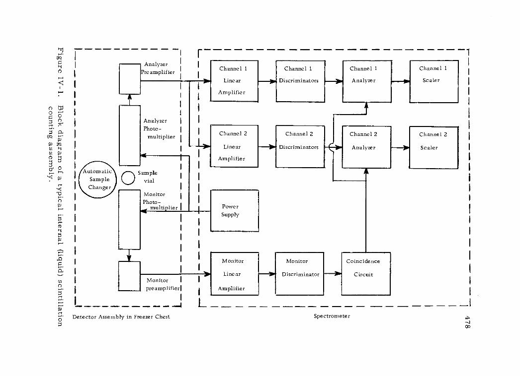
I -A
I aa
n2i3
Analyzer
Pre amplifier
I
I
1
Analyzer I
Photo- I
multiplier I
I
------ --- - -1 Channel
I
»I
1
1
Linear
Amplifier
Channel 1
Discriminators
Channel 1
Analyzer
Channel 1
Scaler >ow
1
1
I Channel 2
Linear
Amplifier
-imp,
Monitor
> Linear Monitor I I
preamplifier) Amplifier
1 ---_-_ Detector Assembly in Freezer Chest
L
Channel 2
Discriminators
Monitor
-III' Discriminator
t
Channel 2
Analyzer
Coincidence
Circuit
Spectrometer
-->
1
I
I
I
i
Channel 2 I
Scaler I
I
1
I
f
1
I
I
1
I
I
I
1
I
n td I
G n I
0° w (
P w I cn t I
cr Automatic p Sample
,r; I Changer rr
w I
I
~t
I
(
4
u) n
r-
Ó
1 I
Sample vial
I I
Monitor Photo-
multiplier I Power Supply
I I I
I
I
I
oo
r-

479
minimize thermal noise. This is normally accomplished by using two
photomultipliers connected by coincidence circuitry and operating the
entire detector in a freezer chest. The use of a pulse height analyzer
with variable discriminator settings is also nearly universal in such
counting assemblies. The following description pertains particularly
to the Tri -Garb Liquid Scintillation Spectrometer Model 314EX series
(Packard Instrument Co. , Inc. , La Grange, Illinois), one of the most
widely used internal - sample scintillation counters currently available.
In addition to the features previously described, it has two independent
pulse height counting channels, each with its own pulse height analyzer
and scaler. Other suitable counting assemblies, such as those manu-
factured by Nuclear- Chicago Corp. , Tracerlab, Inc. , and Baird -
Atomic, Inc. , will have slightly different features.
A. Component Functions of an Internal -Sample (Liquid) Scintillation Counting Assembly
1. Power supply
This component is essentially the same as that described for
the external- sample scintillation counter in Experiment III. The fact
that it supplies a d -c potential to two photomultipliers instead of one
is perhaps the only significant difference.

2. Scintillation detector assembly
480
The entire detector assembly is normally enclosed in a heavy
lead shield and operated in a freezer chest. These two features re-
duce external background radiation and photomultiplier noise levels,
respectively. Models equipped with automatic sample changers have
a turntable and elevator component mounted over the detector. This
allows sample vials to be automatically inserted into and removed
from the sample chamber without light leakage to the photomultipliers.
The detector itself includes a pair of photomultipliers which
view the sample vial from opposite sides. One photomultiplier, the
"analyzer ", passes its pulses into the two counting channels (see
Figure IV -1). The other photomultiplier, the "monitor'. , is used only
to operate the coincidence circuitry. The sample vial contains the
radioactive sample material, a solvent, and fluor solutes. Energy
dissipated in the solution by ionizing particles emitted from the sam-
ple is converted to photons which pass to the photomultipliers and
give rise to output pulses. A preamplifier attached to each photomul-
tiplier base provides initial amplification of these pulses.
3. Linear amplifiers
The signals from the analyzer tube pass to the channel I and
channel II amplifiers, while signals from the monitor tube reach the
481
monitor amplifier. These amplifiers must provide linear amplifica-
tion and must possess good overload characteristics to amplify faith-
fully small pulses in the presence of large pulses. In addition, the
stability of the amplifiers is critical, since any amplifier drift will
result in unreliable counting results. The gain of these three ampli-
fiers is individually adjustable to allow optimal settings in either count-
ing channel when two different isotopes are being assayed simultane-
ously.
4. Discriminators, analyzers, and coincidence circuit
Five discriminators are used in this counter -- two for each
of the counting channels and one for the monitor channel. The two
variable discriminators in each counting channel pass on to the ana-
lyzer only those pulses whose heights lie between their settings. This
voltage interval between the upper and lower discriminators is called
the "window ". The windows in the two channels may be overlapping,
adjacent, or disjunctive, since they may be set independently of one
another. The discriminator in the monitor channel rejects all pulses
below a given level. Usually these pulses are a result of thermionic
or preamplifier noise.
If an output pulse from the monitor amplifier exceeds the vol-
tage setting of the monitor discriminator, a signal passes into the

482
coincidence circuit which serves to open a pathway through the two
counting channel analyzers for a given duration (,-,-,5 mµ sec). If dur-
ing this period a pulse passes through Channel I which exceeds the
lower discriminator setting, but is smaller than the upper discrimina-
tor setting, it can pass on through the analyzer and be registered on
the Channel I scaler. Similarly, pulses in the Channel II window
could pass to the Channel II scaler. Thus, detection requires a mini-
mum of two photons to be emitted by the fluor within the counter re-
solving time.
On the other hand, if a thermal noise pulse were to originate in
the analyzer photomultiplier without the monitor channel being actu-
ated, the signal would be blocked at the analyzers for lack of a sig-
nal from the coincidence circuit. Only when a thermal noise pulse
originates simultaneously in each photomultiplier within the resolving
time of the circuits can such a spurious noise count reach the scalers.
Since thermal noise is random and the counter resolving time is of
the order of 10 -7 seconds, the number of such counts is negligible.
5. Scalers
These components are similar to those previously described
for other counting assemblies. Due to the very short resolving time
of the liquid scintillation detector, the register is entirely based on

483
"glow" tubes, rather than including a mechanical register. A high
speed electronic timer with provision for presetting the counting time
is commonly included.
Automatic scintillation counters are used where large numbers
of samples must be assayed routinely. These counter assemblies in-
clude a console unit to control the automatic sample changer, interro-
gate the scalers and timer at the end of each sample assay, and actu-
ate the associated digital printer. This latter component prints out
the scaler and timer readings for each sample counted to provide a
permanent record. These components and the scalers, analyzers,
coincidence circuit, discriminators, amplifiers, and the power supply
are commonly housed together in a single chasis and termed the
"spectrometer."
B. Operation of an Internal - Sample (Liquid) Scintillation Spectrometer
1. General instructions
This counter assembly is considerably more complex and ex-
pensive than those operated in the past three experiments. Therefore,
it is even more essential to become thoroughly familiar with the manu-
facturer's specific operating instructions before attempting to use the
counter. Since there are a number of adjustable controls on this

484
spectrometer (gain on each amplifier, photomultiplier high voltage,
discriminator settings, counting mode selectors, etc. ), and since the
counting results are only meaningful when these control settings are
stated, it is of the utmost importance to record each control setting
at the time each assay is made.
2. Beta pulse spectrometry
Pulse spectra of beta emitting nuclides of three different en-
ergy levels will be determined for comparison. H3 (Emax 0. 018 Mev),
0. 157 Mev), and C1 36
(E 0. 714 Mev) are suggested as C14 (E max max
covering a suitable energy span. Four individual samples of equal
volume should be prepared as follows:
a. The scintillation solution is made up with toluene as
the solvent, PPO (4 g/1 . ) as the primary fluor, and
POPOP (0. 05 g/1.) as the secondary fluor. The
quantity of solution required will depend on the size
of the counting vials used.
b. Each sample vial should be filled with an equal
measured volume (usually 15 ml) of the scintillation
solution. One vial will have no radioactive sample
and will be used in making background determina-
tions.
485
c. A trace amount (less than one mg) of benzoic acid - C14
(approximately 0. 03 µc), benzoic acid - H3 (approximately
0. 1 µc), and - benzene hexachloride - C136 (about 0. 02 µc)
should be weighed out and added to the three remaining
vials, respectively. Although benzoic acid is a quenching
agent, it may be weighed out with greater precision than
attends the pipetting of liquid samples, such as labeled
toluene. The latter compound (or naphthalene -C14) how-
ever, should be used for counter calibration.
The spectra of each of these four samples should now be deter-
mined at several different photomultiplier potential settings. This can
be done at a given voltage setting ( "tap ") by maintaining a constant
"window" width of five volts in one of the counting channels and mak-
ing successive activity determinations from 5 - 100 v. across the
pulse height scale. Why is a measurement not made with the window
setting of 0 - 5 v? It would be desirable to make such spectrum de-
terminations at photomultiplier potential increments ( "tap settings ")
of about 100 v, but time may not allow this. A family of spectral
curves for each sample should be plotted from the data thus secured
(see Figure 6 -6).
486
3. Selection of optimal counter settings
From the data of the previous section the optimal window and
photomultiplier high voltage settings should now be selected. The op-
timal settings (the "balance point ") for each isotope will be those that
give a maximal value for the expression efficiency2 /background.
Alternatively, the "balance point" setting can be determined empiri-
cally from data as shown in Figure 6 -5. The approxirra to counting
efficiency for any photomultiplier potential and window width can be
estimated from the area included under the curve at those settings.
The area under the background curve for the same settings must also
be considered. The optimal counter settings will not be the same for
each of the three isotopes.
It should be clearly noted that although a wider window setting
results in an increased counting efficiency in most cases, it may also
lead to a much greater increase in background count rate. In addition,
it will be seen from the curves that increased photomultiplier high vol-
tage spreads the spectrum across the pulse height scale, while de-
creased high voltage compresses it at the lower energy ranges. While
it will not be necessary to prepare a family of curves as in Figure
6 -5 to determine the optimal counter settings in this experiment, it
may be necessary to do so in order to achieve greater precision in
certain experiments.
487
In counting situations where quenching is a seri-
ous problem, it would be well to consider the feasibility of "flat spec-
trum" counting. For a more detailed consideration of this concept,
the reader is referred to pages 217 -220.
4. Determinations of efficiency at optimal counter settings
The counting efficiency at the optimal counter settings (balance
point) should now be determined for each of the three isotopes used in
Section 2. This will be done by the internal standardization or
"spiking" method (see pages 221 -222). Each sample is first assayed
at the above determined optimal counter setting. Then, precisely
measured amounts of calibrated standard source compounds should be
added to each sample vial and the vials recounted.
It is suggested that toluene -C14 (about 0. 03 pc), toluene -H3
(about 0.1 µc), and IX- benzene hexachloride -C136 (about 0. 02 µc) be
used as the internal standards. The pipetting of the labeled toluene,
although difficult, must be done with the utmost precision. From the
counting data thus derived the counting efficiencies are calculated ac-
cording to Equation 6 -1. What relationship, if any, exists between
the Emax of the three isotopes and their counting efficiencies? How
do the counting efficiencies of the original C14- and H3- labeled ben-
zoic acid samples compare with the counting efficiencies of the

488
C14- and H3- labeled toluene "spikes "? Does this indicate any quench-
ing effect by the benzoic acid?
5. The effect of a quenching agent
First count each of the foregoing samples under "flat spectrum"
conditions (a window of 10 - 100 v. and the maximum photomultiplier
potential). Then add to each of the counting samples 0.1 ml. of chlo-
roform (a quenching agent) and recount each at the balance point and
under flat spectrum conditions. Add two additional 0.1 ml. amounts
of chloroform and count the samples after each addition under the two
types of counter settings specified. From the data, plot curves of
counting rate vs. chloroform concentration (from 0 - 0. 3 ml. ) for
each of the isotopes at the two counting modes. What can be concluded
from these curves as to the relative quenching effect under balance
point as compared to flat spectrum conditions? What relationship, if
any, exists between the extent of quenching and the Emax of the three
isotopes?
6. Preparation of gel counting samples
Homogenized tissues, water solutions, and solid organic and
inorganic salts have been counted as gel samples (see pages 282 -285).
For this experiment it is suggested that a 0. 5 ml. aqueous solution of
489
an available water soluble organic compound, such as glucose -U -C14
be utilized. (Why would toluene-C1 4 not be satisfactory?) The acti-
vity level should be about O. 01 - O. 02 µc. The required quantity of
gel is prepared by adding sufficient Thixcin (Baker Castor Oil Co. ) to
a toluene solution containing PPO (4 g /l) and POPOP (1 00 mg /l) to
produce a concentration of 25 g /1. Mix the resultant gel for about ten
minutes in a blendor. The labeled sample should be added to a meas-
ured amount of gel (usually 1 5 ml) in a counting vial and thoroughly
mixed by shaking. The balance point settings for this counting sample
and the pulse spectra at a medium and high photomultiplier potential
settings should then be determined. Flat spectrum counting is parti-
cularly suitable for gel samples. How do the pulse spectra of this gel
sample compare with the pulse spectra of the C 1 4 -labeled scintillation
solution determined in Section 2?
C. Summary
The effect of photomultiplier potential and window width on the
counting efficiency of the liquid scintillation counter must be consi-
dered in determining the optimal counter settings (balance point).
Counting efficiency is also clearly related to the beta energy of the
isotope in the sample. Quenching agents in only low concentrations
may drastically reduce counting efficiency. The extent of this

490
decrease in counting efficiency may be determined by internal standar-
dization and minimized by use of flat spectrum counting.
491
EXPERIMENT V - THE NATURE OF RADIOACTIVE DECAY
When a radioisotope shows a significant decay over a reasonably
short period of time, its half -life may be determined by direct obser-
vation. Repeated activity determinations may be made and the data
plotted against time. The half -life is readily found from the graph as
the time required for the initial count rate to decrease by a factor of
two. In this experiment two such half -life determinations are to be
made. One is on the fission produced nuclide I131 and the other on
the very short lived isotope I128. The latter will be produced for this
purpose by the Szilard -Chalmers reaction using a neutron source or
training reactor.
A. Determination of the Half -Life of I131 from a Decay Curve
1 31 From a stock solution of NaI tranfer by pipette about O. 005
µc of I131 activity to a planchet. This sample should then be dried
slowly using a heat lamp. Excess heating should be avoided. If a G-
M counter is to be used for assay, it is necessary to place the planchet
on the shelf of the sample holder which allows an initial count rate of
less than 3, 000 cpm. Why? This will not be necessary if a NaI(T1)
crystal scintillation detector is used.
Determine the net count rate of the I131 sample, collecting a

492
minimum of 10, 000 counts, and record the exact time of the counting.
This procedure should be repeated daily, if at all possible, over a
period of 7 - 10 days. A minimum of five such determinations must be
made. It is essential that the same counter and geometry be used for
every determination. If time allows, a long -lived reference source
should be counted just after each sample assay. In this way any varia-
tion in counter efficiency will be recognized and the sample count rates
can be adjusted accordingly.
Plot the counting data against time on semi - logarithmic graph
paper with the initial count taken as time zero. Draw a straight line
through the points and determine the half -life. An accepted value for
the half -life of 1131 is 8. 066 f 0. 016 days. How closely does your
graphically determined value come to this? For a more detailed dis-
cussion of half -life and radioactive decay, see Chapter 2. Other
readily available nuclides with half -lives of a few days could be used
in place of I131 such as Au198 (2. 697 days), Bi210 013 days), or
P32 (14. 22 days).
B. Preparation of 1128 by the Szilard -Chalmers Reaction and Determination of Half -Life
1. Preparation of I128
The unfortunate consequence of the (n, ) process of Ó
(5.
493
radioisotope formation is that the product atoms are isotopes of the
precursor atoms and thus not chemically separable from them. In 1932,
L. Szilard and T. A. Chalmers demonstrated that after neutron irra-
diation of ethyl iodide, most of the 1128 formed could be readily ex-
tracted with water. This was evidence that the iodine - carbon bond
was ruptured as a result of the I127 Ó
1128 reaction. This altera-
tion of the chemical form of a compound upon activation allowing sub-
sequent chemical separation of the product has come to be known as
the Szilard- Chalmers process. The largest amount of work in the
field of Szilard- Chalmers separations has been done on organic ha-
lides. In this experiment the original work of Szilard and Chalmers
with ethyl iodide will be followed.
Three basic conditions must be met to make a Szilard-
Chalmers separation possible: (1) Following its formation by neutron
absorption, the radioactive atom must emit a gamma ray and recoil
with sufficient energy to break the bond between it and the parent mole-
cule; (2) it must neither recombine with its parent molecule nor ra-
pidly exchange with inactive atoms of other target molecules; and (3)
a chemical method of separating the target compound and the radioac-
tive material in its new chemical form must be available. Since recoil
energy may reach several hundred electron volts, while most chemi-
cal bond energies are in the range of 1 - 5 ev, there will be more than
494
enough recoil energy to break the C -I128 bond. Recombination or ex-
change of the "hot" atoms with inactive atoms of other target mole-
cules is prevented by the addition of a small amount (but large in corn-
128 parison to the amount of I present) of inert I2 carrier. The aque-
ous extraction of the I128 is greatly enhanced by the addition of iodide
ion (as KI).
The following procedures are designedfor use where a nuclear
reactor with a neutron flux of about 106 neutrons /cm2 /sec is obtain-
able (such as the AGN 201 model). Adaptations for use with a Ra -Be
neutron source can be readily made. A suitable amount (about 5 ml. )
of ethyl iodide should be poured into a polyethylene vial and the capped
vial placed in the reactor holding rod. The rod should then be inserted
so that the vial is in the center of the neutron flux (the "glory hole ").
If activation is carried out for 25 minutes (one half -life), the antici-
pated 1128 activity will be sufficient for the present experiment. At
the end of this irradiation period (note the time), the rod should be
withdrawn and the vial removed with tongs and carried to the labora-
tory.
The vial should be placed behind shielding material (I128
emits beta particles with a 2. 12 Mev Emax' as well as assorted gam-
ma rays) and the cap removed. Transfer exactly 1 ml of the ethyl
iodide by pipette to a clear polyethylene vial with an attached cap.

495
Using a clean pipette, add exactly 1 ml. of a solution containing ten
mg KI per ml distilled water to the sample. Cap the sample vial, and,
using tongs, shake the two phases for about 30 seconds. After the
layers separate, carefully open the vial. By means of a micropipette,
transfer 200µ1 of the upper aqueous phase to a stainless steel cup
planchet. Evaporate the sample to dryness under a heat lamp and
cover the dried deposit with mylar film or cellulose tape.
2. Determination of the half -life of 1128
The assay of sample activity using a G -M counter should begin
immediately. Record the time that counting starts. The background
count rate should have been previously determined. Without stopping
the counting, record the register readings at successive one minute
intervals for a minimum period of 30 minutes. For greater precision,
the time of each one minute count should be recorded as the mid -point
of each determination. Due to the short half -life of I128, the counting
rate will drop off appreciably over the total assay period with a result-
ing decrease in statistical accuracy. The counting data should be plot-
ted against time on semi -log graph paper. Time zero is taken as the
time the activated sample was removed from the reactor. Graphically
determine the half -life of 1128 from the observed values. By extrapo-
lation, determine the total measurable activity in the 200 µl sample
496
at time zero.
3. Determination of G -M counter coincidence loss using I128
If time permits, the coincidence loss of the counter can be
determined by the employment of a larger 1128 sample, such that the
initial count rate is about 10, 000 cpm. Assay of this activity level
with a G -M counter will result in an observed count rate considerably
less than the "true" count rate, due to coincidence loss. With subse-
quent decline in activity, the degree of coincidence loss will decrease
until eventually a true exponential decay curve will be observed. Ex-
trapolation of the linear portion of the curve back to time zero will
give the "true" initial count rate. The difference between this and the
observed count rate will represent counter coincidence loss.
497
EXPERIMENT VI - INTERACTION OF RADIATION WITH MATTER
Some aspects of the interaction of the various types of radia-
tion with matter were discussed in Chapter 3. In this experiment two
aspects of interaction will be considered as they relate to radiotracer
assay. One is the external absorption of beta and gamma radiation in
aluminum and lead, respectively, and the second is self -absorption in
counting samples of weak beta -emitters.
A. External Beta Absorption
1. Theory
A standard method in the characterization of beta radiation is
the preparation of absorption (transmission) curves (see Figure 3 -9).
This is typically done by inserting a series of aluminum absorbers
between a pure beta -emitting source and a detector up to thicknesses
exceeding the beta particle range, and observing the counting rate for
each thickness of absorber. The logarithm of the observed activity is
then plotted against absorber thickness. In general, such absorption
curves are not highly precise, but a rough value of the range and
E of the beta particles involved can be derived from them. max
In order to ascertain the E of a beta - emitter from an max
498
absorption curve it is necessary to first determine the range accurate-
ly. Range determination from an absorption curve is attended with
considerable uncertainty. Although the curve will appear nearly ex-
ponential over much of its length, it commonly deviates from linearity
at both ends. The production of Bremsstrahlung (see p. 85) largely
accounts for a flattening of the curve near the limit of range. In addi-
tion, the shape of the absorption curve varies somewhat with the geom-
etry of the arrangement in which it is measured, because of the contri-
bution of scattering effects.
A rough, though inaccurate, estimate of range can be made by
simply extrapolating the linear portion of the absorption curve to the
abscissa. In some cases the curve will be found to turn downward
from the linear portion and to intersect the abscissa vertically at a
point which may be taken as the visual range. (It should, of course, be
remembered that the abscissa intercept does not have the same mean-
ing on a semi -log plot as on a linear plot. ) Beta range may be alter-
natively determined more precisely, but with a greater expenditure of
time, by methods such as the Feather analysis (see references 3 and 7
in Chapter 3). Absorption methods for the precise determination of
beta range have been superceded by the employment of the beta ray
spectrometer with which direct beta energy measurements may be
made.
499
The E max of a beta - emitter can be calculated from the meas-
ured range by the empirical relation developed by Glendenin, as fol-
lows:
(Equation VI -1) E max (Mev) = 1.85 Range (g /cm2) + 0. 245
This equation is reasonably valid for ranges greater than 300 mg /cm2.
2. Procedure
A counting source of a pure beta - emitter of reasonably high en- 32
ergy, preferably P , should be prepared by evaporation on a planchet.
It should be of sufficient activity to show 5, 000 - 10,000 cpm when
placed on a lower shelf of the sample holder. A thin end - window G -M
detector of known window thickness should be mounted in a fixed rela-
tion to the sample. Neither detector nor sample should be moved dur-
ing the experiment. A set of calibrated aluminum absorbers will be
required.
The optimal arrangement is to place the absorbers as near the
detector window as possible, and the source somewhat farther away.
The sample counting rate should now be determined with no absorber,
and then with absorbers of increasing thickness until the counting rate
is decreased to background or becomes constant. It will not be practi-
cal in the limited time available during a laboratory period to maintain
a constant statistical accuracy in counting. Normally longer counting
500
times would be required with the thicker absorbers in place. The
length of each activity determination can be determined, then, by the
time available, not statistical considerations.
The observed sample activity must be corrected for background
and coincidence loss (see Experiment I). Plot the corrected activities
against absorber thickness on semi -log graph paper with the appro-
priate number of cycles. In locating the origin allow room for extra-
polation of the curve to the left. In order to extrapolate activity to
zero absorber, the contribution of air and detector window absorption
must be considered (see Figure 9 -7). The distance between source
and detector window should be measured. Air density may be taken as
1. 2 mg /cm2. The thickness of the G -M tube end - window will be found
in the information supplied by the manufacturer.
From the extrapolated absorption curve estimate the range of
P32 beta particles in aluminum. Find the E max for this emitter by
Glendenin's equation. How do these experimental values compare to
the recognized values for P32 of a 790 mg /cm2 range in aluminum and
an E max of 1. 71 Mev? Why might the experimental values differ con -
siderably from the accepted values? What bearing does this aspect of
beta particle range have on the problem of shielding high levels of beta
activity?
B. External Gamma Absorption
1. Theory
501
The subject of gamma ray absorption was fully discussed in
Chapter 3 (pages 95 -114), and it is suggested that the reader familiar-
ize himself with that discussion before proceeding with this experi-
ment. It will be recalled that the interaction of gamma photons with
matter is markedly different from that of charged particles. Gamma
rays (as well as x -rays) show a characteristic exponential absorption
and have no well defined range.
In this experiment a gamma absorption curve in lead will be
prepared. From this plot the mass half -thickness (the absorber thick-
ness that reduces the incident gamma intentisy by a factor of two) can
be directly determined. The mass absorption coefficient can then be
calculated from this value according to the relation:
(Equation VI-2) 0. 693
x - 1 µm 2
(see Equation 3 -13)
Also, from the experimentally determined value of X1 the approxi-
mate gamma energy can be found using Figure 3 -1 8.
502
2. Procedure
The only difference here as compared to the previous absorp-
tion experiment with a beta -emitter is the placement of the detector,
absorbers, and the counting sample. The geometry of the counting
arrangement is particularly critical for gamma detection, since the
photons are so readily scattered. Ideally the gamma rays should be
collimated by placing the prepared source at the bottom of a lead well
whose opening faces the detector. The source and the detector should
be separated by as great a distance as the sample activity will allow,
but at least two inches. The lead absorbers will be inserted midway
between the two. It is desirable to place an aluminum absorber of
about 1 g /cm2 close to the detector to absorb any secondary electrons
ejected from the lead absorbers.
Suitable counting sources are those which emit gamma rays of
a single energy (Cs137) or of very similar energies (Co60). A set of
calibrated lead absorbers with thicknesses up to 25 g /cm2 will be
needed, although aluminum absorbers may be used at the start. The
detector may be either a G -M tube or a NaI(T1) crystal scintillation de-
tector. The required activity of the counting source will depend on the
detector type employed.
Counting rate determinations for the various absorber
503
thicknesses should be made as described above. Then plot the net ac-
tivities on semi -log graph paper against absorber thickness. Is the
resulting curve linear? From the most linear portion of the curve
determine the mass half -thickness. Using this experimental value
calculate the mass absorption coefficient and find the gamma energy
as described above. How do these experimental values compare with
corresponding published values for the nuclide used?
C. Self- absorption in a Weak Beta - emitting Sample
1. Theory
The effect of self- absorption on sample radiation has been dis-
cussed in Chapter 9. Self- absorption is primarily a problem in the
assay of low energy beta- emitters, where variations in sample weight
and specific activity exist. This effect will be examined in this experi- 14
ment as it concerns samples of BaC 03 of the same specific activity,
but differing thickness. One of the commonest methods of compensat-
ing for differences in self- absorption from sample to sample is the use
of a self- absorption correction curve. Such a correction curve will
also be prepared from the experimental data. It should be understood
that a separate curve must be prepared for each nuclide and molecular
type assayed, and that a curve is only valid for the counting assembly
504
and geometry used in its preparation. For uniformity in the mounting
of the solid counting samples to be used the method of slurry centri-
fugation will be employed here (see Chapter 8).
The observed specific activity of a BaC14O3 sample will ap-
proach the true specific activity in only the thinnest of samples. How-
ever, there is considerable difficulty in securing uniformity in such
very thin samples. A more precise means of determining true speci-
fic activity (zero self- absorption) is to plot the apparent specific acti-
vities (cpm /mg) of a series of BaC14O3 samples of different thickness
against sample thickness and extrapolate to zero thickness. Using
this value of the true specific activity as 100 percent, a second plot is
made of the percentage specific activity at each thickness (apparent
specific activity /true specific activity) against sample thickness (mg/
cm2). This plot serves as a correction curve for self -absorption in
BaC14O3 samples. The apparent sample specific activity for any
thickness (below "infinite" thickness) can then be graphically convert-
ed to the true specific activity, and hence to total sample activity.
When counting sample thickness becomes greater than the
range of the beta particles it emits, only the radiation from the upper
layer will be detected. Addition of more of the same sample will not
affect the count rate. Such a sample is known as possessing saturation
thickness, or being "infinitely" thick. Under these conditions the
505
counting rate of the sample will be directly proportional to the specific
activity of the sample, not to the total amount of activity in the sample.
Many workers prefer to count infinitely thick samples, if sufficient
amounts of sample are available, to thus avoid self- absorption correc-
tions. Any samples in an experimental series that are less than satu-
ration thickness are then corrected to that thickness graphically for
the sake of comparison.
2. Procedure
A stock solution of Na2C 1403 (1 00 ml) should be prepared con-
taining 5 mM Na2CO3 with a specific activity of about 3, 000 cpm /mM.
The stock solution should be dispensed into ten Erlenmeyer flasks in
the following amounts: 30, 20, 10, 8, 7, 6, 5, 4, 3, and 2 ml. Warm
these flasks on a water bath to 70 °C and then add to each two ml of
the precipitation mixture (1N NH4C1 and 1N BaC12). Stopper and gen-
tly agitate the flasks.
After cooling, the contents of each flask should be transferred
quantitatively to plastic centrifuge tubes, using water to effect the
transfer. Centrifuge the samples for four minutes at full speed. The
resultant supernatant may then be decanted into a radioactive waste
can. Add 70 percent alcohol to the residue in each tube, stopper the
tubes with rubber stoppers and shake violently to resuspend the
506
BaCO . Transfer the alcohol suspension quickly to the special stain - 3
less steel centrifuge tubes (supplier is Atomic Products) holding pre -
weighed aluminum planchets. Rinse any residual BaCO3 from the plas-
tic tubes with alcohol. The stainless steel tubes are balanced with al-
cohol and immediately centrifuged at full speed for six minutes.
After centrifugation the tubes should be removed and the alcohol
decanted immediately. With the centrifuge tubes inverted planchet
side up, each O -ring is pried out and the planchet removed. The sam-
ple planchets should be dried slowly under a heat lamp and then stored 14
in covered Petri dishes. To remove traces of BaC O rinse all the 3
equipment used in dilute HC1 in a hood, and then in tap water to remove
the HC1.
Weigh each planchet and calculate net sample weight. Each
sample planchet should be assayed twice to a standard deviation of less
than one percent with a G -M tube or proportional detector. From the
area of the planchets calculate the thickness of each sample in mg /cm
Now plot the net counting rate for each sample against the respective
sample thickness. Compare the resultant curve with Figure 9 -8.
Does it appear that any of the samples are of saturation thickness?
In order to prepare the self- absorption (transmission) correc-
tion curve, calculate the apparent specific activities for BaC14O3 on
each planchet (cpm /mg). Plot the respective apparent specific
507
activities against sample thickness on semi -log graph paper. Extra-
polate this curve to zero thickness and consider the value as the true
specific activity. Now, using the value of the true specific activity as
1 00 percent, plot the percentage specific activity observed at each
sample thickness against thickness. Can the saturation thickness val-
ue be determined from this plot? This plot should be preserved for
possible later use in assay of BaC14O3 samples with the same counting
assembly and geometry.
508
EXPERIMENT VII - STATISTICAL CONSIDERATIONS IN THE MEASUREMENT OF RADIOACTIVITY
This experiment is designed to illustrate the statistical consi-
derations discussed in Chapter 9. It is suggested that that chapter be
consulted in connection with the calculations at the end of the experi-
ment.
A. The Normal Distribution of Counting Results and Error Probability
Place a suitable radioactive source in a fixed relation to a ra-
diation detector so that a counting rate of 2, 000 - 2,500 cpm is obtain-
ed. G -M, proportional or external scintillation counters, are equally
suitable for this purpose. In the case of the latter two counter types
a much higher count rate can be tolerated. Why? Make a series of at
least 20 consecutive observations (more would be preferable, if time
permits) of one minute duration each. The source should not be dis-
turbed during these measurements.
Record the total number of counts (n) collected in each obser-
vation without making any correction for background or coincidence
loss. These results will then be used to compute the standard devia-
tion by calculating in order the following values:
(a) The mean total count (ñ), that is the sum of all the counts
divided by the number of observations (N).
509
(b) The algebraic deviation (0) of each observation from this
mean count (O= n - ñ).
(c) The square or the deviations of each observation
(d) The sum of the squares of the deviations (EA2)
(e) The standard deviation (0-), that is the root mean square
EQ2 N
(f)
deviation o
The algebraic sum of the deviations (EA), which should be
very nearly equal to zero.
(g) The approximate standard deviation, that is the root mean
(o- = Nrri
(h) The percent standard deviation (relative o- ), that is the
reciprocal of the root mean (relative o- = WTI). ).
Examine the observations for closeness of fit to a normal dis-
tribution as follows:
(1) Compare the approximate o- as calculated in (g) to the
precise value of o- from (e). They should be equal or
very nearly equal.
(2) Determine the number of observations showing deviations
greater than 1 a- (using the exact o- value). This should
occur in approximately 1/3 (31. 7 percent) of the observa-
tions.
( 4 .
_
510
(3) Similarly determine the number of observations showing
deviations greater than 2 o-. This should occur in about
one observation in 20 (4. 6 percent).
Precise agreement to the above values is not to be expected, because
of the relatively small number of observations.
B. Rejection of Suspected Data
Considering the data in Part 1, determine if any of the activity
measurements deviate so greatly that they should be discarded accord-
ing to the following criteria:
(a) The observation differs from the mean by more than 2 o-
(b) The observation differs from the mean by more than 3 0-
(c) The ratio of the deviation to the standard deviation exceeds
the appropriate value in Table 9 -3 (Chauvenet's criterion).
Explain how an observation might be rejected on the basis of one of
the above criteria, but not on others. Which of these critera is the
most lenient, that is, would tend to include observations with the
greatest deviations?
.
.

PART THREE
SELECTED RADIOTRACER
EXPERIMENTS

511
EXPERIMENT A - INCORPORATION OF C1402 INTO AMINO ACIDS IN YEAST
This experiment has been selected to illustrate the utilization
of C14 as a tracer in microbial metabolism. Specifically, it involves
tracing the fate of C140 in amino acid metabolism in yeast cells. 2
14 The C 02 is administered in the gaseous state in a closed system,
although it could as well be supplied as HC 1 4
O 3
in solution in the
culture medium. The amino acids in hydrolysates of the yeast cells
are separated by paper chromatography and the C14 label detected
by autoradiography. The pattern of amino acid labeling can serve
as a clue to the mechanism and role played by CO2 in the metabolism
of microorganisms. Under the experimental conditions specified,
the results will be largely qualitative rather than quantitative.
The experimental procedure has been covered in an especially
detailed fashion, so that individual students can carry out the steps
with little or no guidance. The materials and reagents needed are
neither excessively costly nor uncommon, so that the experiment
can be carried out in almost any bacteriological laboratory. The
step -by -step calculation of the amount of C 14 needed illustrates the
type of experimental design required in radiotracer experiments.
2
A. Survey of the Problem
512
It is well known that microorganisms generally produce and
liberate CO2 as a result of their metabolic processes. It is equally
clear that photosynthetic microorganisms remove from their environ-
ment and utilize CO2. In addition, some non -photosynthetic CO2
fixation is carried on by many microorganisms. This process has
been studied in only a moderate number of species (3).
Such CO2 incorporation can be readily followed if the carbon
used is radioactive C14. The C14- labeled metabolic products can
then be separated and identified by use of the techniques of paper
chromatography and autoradiography. It is the appearance of C14-
labeled amino acids that will be followed in this experiment. Of
course, other labeled products also occur, chiefly organic acids.
This experiment demonstrates how such techniques can be applied to
the study of a specific organism - -- Saccharomyces cerevisiae
(Baker's yeast). Davis, et al.(2), and Stoppani, et al. (5), have pre-
viously traced CO incorporation into amino acids in yeast. 2
Briefly, the experiment consists of the following major acti- 14
vities: (1) Exposure of a known amount of yeast cells to C 02
generated in the reaction vessel; (2) Removal of residual C1402,
followed by separation and hydrolysis of the yeast cells;
513
(3) Development of one -dimensional paper chromatograms from
measured aliquots of the yeast hydrolysate and amino acid reference
standards; (4) Detection of labeled compounds on the chromatograms
by autoradiography; and (5) Determination of the pattern of amino
acid labeling as well as the relative quantities of C14 incorporated
into the various amino acids by comparison of the chromatograms
and autoradiograms.
B. Experimental Design
In the calculation of the amount of radioactive material to be
used in this experiment certain assumptions must be made. These
may be subject to some error and for this reason are conservative.
The assumptions are in accord with experimental results (2, 5).
Since the goal of the experiment is to determine C14 labeling
of various amino acids by autoradiography, the amount of C14 to be
used is based on the assumed amount fixed in a specific amino acid.
Aspartic acid has been chosen for the following calculation. The
reader is referred to Chapter 10 for the rationale behind this method
of calculation.
(1) The optimal amount of a substance on a chromatogram
spot is usually chosen to be ten micrograms.

514
(2) To produce a good image on x -ray film in a reasonable
time (about a week), a one square centimeter spot on the chromato-
gram should show about 1 00 cpm when assayed with a thin end - window
G -M detector placed directly over the spot.
(3) Assuming about ten percent efficiency of the G -M detector
for assaying C14 in these spots, this is:
100 cpm 1 0% efficiency = 1 , 000 dpm per cm2 spot
(4) Since each spot is to contain about ten micrograms of
aspartic acid, this amounts to a specific activity of:
1 , 000 dpm /cm2 spot
1 0 µg /cm2 spot 100 dpm /µg aspartic acid
(5) If it is assumed that about five percent of the dry weight
of the yeast cells is aspartic acid, and a yeast sample of about 20
milligrams dry weight is required, there would be:
20 mg yeast x 5% aspartic acid in yeast = 1 mg aspartic acid in sample
(6) Then the required total amount of activity in the aspartic
acid would be:
1 , 000 µg aspartic acid x 100 dpm /µg aspartic acid
= 105 dpm /mg aspartic acid
(7) If it is further assumed that under the conditions of this
experiment about 20 percent of the total Cl 402 fixed will be found
515
in aspartic acid, then: 5
1 0 dpm fixed in aspartic acid 5
0. 2 of total fixation in aspartic acid 5 x 10 dpm in total yeast sample
(8) Assuming that only about one percent of the Cl 40 in the 2
reaction vessel will be fixed by the yeast cells, the total activity re-
quired for this experiment is:
5 x 1 05 dpm in total sample 0. 01 fixation in sample = 5 x 10⁷ dpm total activity
required
This amount is equivalent to about 20 microcuries of C14
C. Materials and Equipment Required
This listing includes only special equipment and reagents used
in the experiment and is not complete. Items are listed in order of
usage.
1. Reaction vessel: As illustrated in Figure A -1 , this consists of
a side flask (25 ml Erlenmeyer) and a test tube (about 10 ml)
joined to a main flask (125 ml Erlenmeyer) Each of the open-
ings should be provided with a tight fitting serum cap. Although
this piece must be custom made, it can be utilized in a wide
variety of radiotracer experiments involving CI 40 . Much more
2
elaborate vessels could, of course, be employed for this purpose.
-
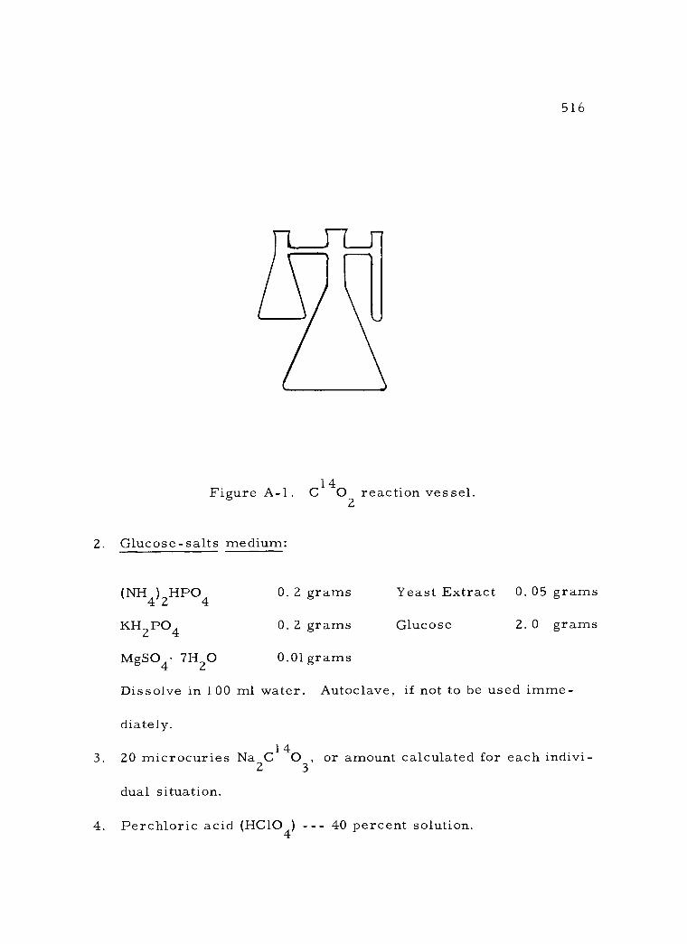
Figure A -1. C140 2
reaction vessel.
2. Glucose -salts medium:
516
(NH4)2HPO4 0. 2 grams Yeast Extract 0. 05 grams
KH2PO4 0. 2 grams Glucose 2. 0 grams
MgSO4. 7H2O 0.01 grams
Dissolve in 100 ml water. Autoclave, if not to be used imme-
diately.
3. 20 microcuries Na2C14O3, or amount calculated for each indivi-
dual situation.
4. Perchloric acid (HC1O4) - -- 40 percent solution.
517
5. Oxygen -gas torch and accessories for sealing pyrex hydrolysis
tubes.
6. Chromtographic equipment - -- jars, racks, troughs, papers, etc.
7. Amino acid chromatography standard solution: The following
amounts of the amino acids specified should be dissolved in 100 ml
of ten percent iso- propyl alcohol. These amounts will provide
0.10 micrograms of oC -amino nitrogen per 2. 5 microliters of solu-
tion (4). Store this solution in a refrigerator.
Aspartic acid 38 mg Glutamic acid 42 mg
Lysine 42 mg Arginine 49 mg
Serine 30 mg Glycine 21 mg
Histidine 44 mg Threonine 34 mg
Alanine 25 mg Proline 33 mg
Tyrosine 52 mg Valine 33 mg
Methionine 43 mg Leucine 37 mg
Phenylalanine 47 mg
8. Chromatographic solvent (4): Prepare by thoroughly shaking
together 120 ml of secondary - butanol (peroxide -free) and 40 ml
of fresh three percent NH4OH. The solvent is then ready for use
or may be stored in a refrigerator.
9. Ninhydrin solution: Prepare by adding 0. 625 grams of ninhydrin
(triketohydrindene hydrate) and 2. 5 ml of glacial acetic acid to
518
acetone and make up to 250 ml with additional acetone. Store in
darkness.
10. Geiger - Mueller counting assembly with a thin end - window detec-
tor (less than 2 mg /cm2) mounted in a probe.
11. Dark room facilities.
12. X -ray fixer, rapid x -ray developer, No- Screen medical x -ray
film (14" x 1 7 "), and x -ray exposure holder (14" x 1 7 ").
D. Experimental Procedure
1. The Cl 40 2
incorporation reaction
The steps in preparing the reaction vessel are as follows: Pi-
pette 50 ml of the glucose -salts medium into the center flask of the
reaction vessel (see Note 1). Next, add 20 mg of commercial dry
yeast to the center flask (see Note 2). With a safety -pipetter add
14 20 µc of Na2C 03 to the side tube. (The pipette will be contami-
nated!) Immediately apply serum caps to all three openings.
Apply a vacuum in the reaction vessel by evacuating air through
a hypodermic needle inserted through the middle serum cap. A
water aspirator pump is sufficient for this task. Then inject about
one ml of 40 percent Perchloric Acid (see Notes 3 and 4) with a
syringe into the side tube to liberate Cl 402 (see Note 5). In order
519
to sweep the C14O into the main flask, quickly introduce a flow of 2
air by inserting a long hypodermic needle deep into the side tube,
but not touching the liquid. Then remove this needle immediately.
Place the reaction vessel on a shaker table for one hour at
about 300 C to allow the fixation reaction to procede adequately. A
longer time can be used with a consequent greater amount of Cl 402
incorporation. Remove the reaction vessel from the shaker and in-
ject about ten ml of 6N NaOH through the serum cap into the empty
side flask to react with and trap the excess C O .
14 Inject about ten 2
ml of concentrated HC1 through the serum cap into the center flask
to drive off the dissolved CI 40 and inactivate the cells. Replace
2
the reaction vessel on the shaker table for about ten minutes to as- 14
sure complete C O trapping. 2
The solution in the side tube may be pipetted out and discard-
ed into the drain. It should not be radioactive, but to check on the
completeness of the CI 40 generation from the original Na C14O ,
2 2 3
a planchet could be prepared for G -M assay.
The solution in the side flask contains the unreacted C14
trapped as NaHC14O . This should be carefully pipetted out and 3
may be saved for other experiments. Wash out the side flask with
two or three small amounts of distilled water and add these washings
to the above solution for storage. If desired, an aliquot of this
520
solution could be placed in a planchet and assayed to determine
roughly the percentage recovery.
2. Preparation of the protein hydrolysate
Carefully pipette out the yeast suspension from the center
flask of the reaction vessel and transfer it to a centrifuge tube.
Centrifuge the yeast suspension at 2,000 to 3, 000 rpm for 15 -20
minutes. Decant the supernatant into a marked liquid radioactive
waste container.
Add about five ml of concentrated HC1 to the tube of centri-
fuged cells and then transfer this suspension quantitatively to a small
pyrex test tube (about 15 ml). Working over a tray, seal the open
end of the test tube in the flame of an oxygen -gas torch. Inspect the
closure carefully to insure that no small openings remain. Allow the
tube to cool before proceeding. It is wise to practice sealing a test
tube of water before attempting the operation with the radioactive
sample.
To prevent any possible loss of radioactive material due to
leakage during hydrolysis, place the sealed tube in a larger test tube
with the sealed end down. Place this, in turn, in a small Erlen-
meyer flask and cover the top of the assembly with a small beaker.
Autoclave this assembly at 15 psi. for 6 -8 hours to completely
521
hydrolyze the cellular proteins to amino acids.
3. Separation of the amino acids by paper chromatography
a. Separating the amino acids: After the hydrolysis tubes
have cooled to room temperature they should be cautiously opened
under a hood. This is done by making a file scratch around one end
of the tube and then touching a red -hot glass rod to the scratch.
Protective glasses and an apron should be worn, as occasionally
some glass shattering occurs.
To remove the carbonized cellular debris (humin), filter
all the hydrolysates with suction through a medium porosity fritted
disc or paper. Wash the hydrolysis tubes and filter twice with small
amounts of water and collect with the sample. Transfer the collected
sample to a small beaker.
Cautiously evaporate off most of the HC1 from the hydrolysate
on a warm water bath, taking precautions against the splattering of
contents out of the beaker. To remove water and the remaining HC1
from the hydrolysate, place the beaker in a vacuum dessicator con-
taining fresh P205 in the bottom and a beaker of concentrated NaOH.
Apply a vacuum and let stand overnight. Remove the beaker with
the amino acid crystals from the dessicator and re suspend them in
exactly one ml of water.
522
b. Developing the chromatograms: Prepare three sheets of
Whatman No. 1 chromatographic paper of 6 x 22 inches in size with
coarse serrations at one end of each (see Note 6). At the other end
draw a line with a pencil across the paper three inches from the end.
The spots should be made along these pencil lines (see Note 7). Mark
these sheets A, B, and C, respectively.
On sheet A place four spots of the yeast amino acid sample
solution in respective amounts of 2. 5, 5. 0, 7. 5, and 10. 0 microliters
with a micropipette (4). No more than 2. 5 microliters should be
added at a time on a spot. Allow this amount to dry, then re spot.
The four spots should be equally spaced along the pencil line at the
upper end of the sheet and a notation made nearby in pencil of the na-
ture and amount of the spot. This sheet will be used later for the
autoradiographic detection of the labeled amino acids and will not be
treated with ninhydrin.
On sheet B likewise place two spots of the amino acid sample
in amounts of 2. 5 and 5. 0 microliters and two spots of amino acid
standard solution (item 7 in section C) in the same amounts. On
sheet C, apply spots as previously, but use 7. 5 and 10. 0 microliter
amounts of both sample and standard solutions. Thus, on the se-
cond and third sheets a direct comparison of the standard and sample
amino acids in various amounts can be made later.
523
Place the three sheets on racks in a chamber prepared for
descending chromatography. After closing the chamber, allow it to
equilibrate with the dish of solvent at the bottom for 1-2 hours. At
that time fill the solvent trough through the hole in the top of the
chamber with the secondary - butanol /ammonia solvent (item 8 in
section C).
The amino acids which move most rapidly down the paper
(leucine and phenylalanine) travel only about one -half to one -third
the speed of the solvent front. Since the solvent front reaches the
bottom of the paper in about 24 hours, it will take 48 -72 hours to
secure maximum separation of the amino acid mixture. Since this
latter time is somewhat unpredictable, it is suggested that sheet B
be removed at about 48 hours and developed to determine the pro-
gress of the separation. The amount of time, if any, for further
movement of the amino acids on the other two sheets can then be
estimated fairly accurately.
Set aside sheet A for subsequent autoradiography (see Note
8). In order to detect the individual spots, first dry sheets B and C
in a hood. When dry, dip them quickly in ninhydrin solution and
again hang them up to dry. Since ninhydrin decarboxylates the
amino acids, some Ci402 will be released. Thus, these steps
should be performed under a hood. The two dried chromatograms
524
are then placed in a warm oven for about 30 minutes to intensify the
colors.
Examination will reveal which one of the sample and standard
amino acids increments used is optimal. By comparison of the col-
ored spots on the sample and standard chromatograms, the amino
acid composition of the yeast hydrolysate may be roughly deter-
mined. Of course, not all the amino acids separated from the hydro -
lysate are radioactively labeled (see Note 9).
The linear arrangement of amino acid spots (in order of in-
creasing movement) on the standard chromatogram is given by
Roland and Gross (4) as follows: aspartic acid -- glutamic acid -
cystine (unresolved), lysine, arginine, glycine- serine (unresolved),
histidine -threonine (unresolved), alanine, proline (reacts with nin-
hydrin to give a yellow spot -- easily overlooked), tyrosine, valine,
methionine, isoleucine, leucine, phenylalanine. In general, the
spots will be equally spaced, except for gaps occurring between
alanine and proline, and between methionine and isoleucine.
4. Detection of the labeled amino acids by autoradiography
For an adequate exposure, a chromatogram spot and the film
should remain in contact long enough for approximately 107 beta
particles per square centimeter to be absorbed by the emulsion.
525
This exposure time can only be roughly calculated. Using a thin
end - window G -M detector, locate the radioactive spots on chromato-
gram A and select one of moderate activity. From the determined
count rate of this spot, the area of the detector window, (see Note
10) and the known C14 detection efficiency of the G -M detector under
similar conditions, calculate the exposure time required to produce
an adequate image on the film. Since the various spots on the chro-
matogram will vary considerably in the amount of C14 they contain,
this calculated exposure time will represent a compromise value.
Using a rubber stamp and radioactive ink mark the chromato-
gram at three points to allow subsequent alignment of it with the de-
veloped autoradiogram. In complete darkness place a 7" x 17"
sheet of x -ray film in an x -ray film holder. Arrange chromatogram
sheet A on it and attach it to the film at both ends with small pieces
of cellulose tape. Close the holder and store in darkness for the re-
quired exposure time, either weighted or clamped tight.
At the end of the calculated exposure time remove the film
in complete darkness. The film should then be developed in x -ray
developer, washed briefly in one percent acetic acid, fixed in x -ray
fixer and finally washed in water for at least 20 minutes. Follow
directions on developer and fixer containers for time and tempera-
ture to be used.

526
The optimal chromatogram of the amino acid standards and
that of the hydrolysate sample should now be placed alongside the
autoradiograms for comparison. The relative amount of radioactive
C14 in each spot on the autoradiogram can be determined by compar-
ing the degree of blackening produced on the film. By comparison
with the chromatogram of amino acid standards the identity of the
radioactive spots can be determined (see Note 11). A table should
be made of the amino acids detected on the chromatograms of the
yeast hydrolysate and the degree, if any, of C14 incorporation found
in them, as judged from the autoradiograms. For further informa-
tion on the mechanism of CO2 incorporation by yeasts see the arti-
cles by Davis, et al. (2), and Stoppani, et al. (5).
E. Experimental Notes
1. Aseptic technique does not need to be rigorously followed
here due to the short growth time and the large number of cells intro-
duced initially. Of course, the glucose -salts medium must be auto-
claved, if prepared well in advance.
2. Many other microorganisms could just as well have been
used (3). It should be repeated that the basic techniques are appli-
cable to such further study with little or no modification. If culture
suspensions are utilized, appropriate calibration must be available
527
to allow calculation of the dry weight of the cell sample.
3. Why was perchloric acid used here, rather than some
more common acid, such as HC1?
4. An interesting variation could be followed here by flushing
the reaction vessel with N2 to determine CO2 fixation under anaero-
bic conditions.
5. If the medium is sufficiently acidic, a solution of
NaHC1403 could simply be added to it directly. The exposure of the
yeast cells to gaseous C1402 generated in a closed system is followed
in this experiment, since this method is of more general application.
It can be employed with mammals and the leaves of higher plants,
where use of HCO - solutions would not be possible. 3
6. If available, the so- called "pinking shears" used by seam-
stresses are useful for this purpose when many chromatograms must
be prepared.
7. The chromatogram sheets should be handled as little as
possible and then by the edges. Otherwise the later development of
the chromatogram will bring out a blur of fingerprints. It is pre-
ferable to thoroughly wash the hands with soap before this part of the
experiment.
8. Why was the chromatogram to be used in autoradiography
not treated with ninhydrin? It may be so treated, if desired, after

528
the autoradiogram has been prepared.
9. If one desires to preserve the ninhydrin- reacted spots,
it is suggested that the chromatograms be stored in a dessicator in a
nitrogen atmosphere in the dark.
10. It is often convenient to prepare a lead shield with a one
centimeter square opening to fit over the end -window of the G -M
detector. In this way the count rate from weak beta -emitters such
as C14 can be determined directly in cpm /cm2. Why would such a
technique not be acceptable for use with I131-labeled chromatogram
spots?
11. If a G -M chromatogram scanner attached to a chart re-
corder is available its record of the radioactive pattern along the
chromatogram sheet would offer a valuable comparison to the auto -
radiogram.
BIBLIOGRAPHY
1. Block, Richard J. , Emmett L. Durrum and Gunter Zweig. A
manual of paper chromatography and paper electrophoresis. 2d. ed. New York, Academic Press, 1958. 710 p.
2. Davis, J. Wendell, et al. Carbon dioxide fixation and biosynthe- sis of amino acids in yeast. Biochimica et Biophysica Acta 21 :1 01 -1 05. 1 956.
3. Lynch, Victoria H. and Melvin Calvin. CO fixation by micro- organisms. The Journal of Bacteriology 63:525 -531. 1952.
529
4. Roland, J. F. , Jr. and A. M. Gross. Quantitative determina- tion of amino acids using monodimensional paper chromato- graphy. Analytical Chemistry 26:502 -505. 1954.
5. Stoppani, A. O. M. , et al. Assimilation of carbon dioxide by yeasts. The Biochemical Journal 70:438 -455. 1958.
530
EXPERIMENT B - A KINETIC STUDY OF THE UTILIZATION OF GLUCOSE -U -C14 BY INTACT RATS BY MEANS
OF AN ELECTROMETER SYSTEM
A most important branch of radiotracer methodology concerns
kinetic studies of respiratory metabolism. The term "radiorespiro-
metry" has been given to this type of investigation. The present
experiment illustrates one type of radiorespirometric study involving
a vibrating -reed electrometer as the detection instrument. With this
instrument a continuous measurement of the C14O respired by a rat
previously intubated with uniformly labeled glucose (glucose- 14)
can be made. By means of an infrared analyzer in the flow system,
the total CO2 respired can also be continuously monitored. From
these two synchronous measurements specific activity can be readily
calculated.
Detailed information is given on the assembly and operation
of a flow system incorporating the above two measuring instruments.
Factors to be considered in the experimental design that are peculiar
to flow measurements are discussed at length. In addition, a series
of research applications for such a measuring system are described
and representative references cited.
2
U
531
A. Survey of the Problem
The rate of catabolism in rats of a labeled substrate can be
followed by detecting the respiratory evolution of C1402. Various
methods of detection have been utilized, most of which depend on
sweeping the expired CO2 out of a respiratory chamber containing
the rat and trapping it in a basic solution. The absorption trap is
changed at intervals and counting samples prepared from the solu-
tion obtained. Sample activity may then be assayed by means of a
G -M counter, a proportional counter, or a liquid scintillation count-
er. The chief drawback of these methods is the extensive time in-
volved in sample preparation and counting, and even then only cumu-
lative interval samples are obtained.
By contrast, the method employed in this experiment allows
continuous and instantaneous measurements of both C1402 and total
CO2 to be made over an extended period of time. The need for sub-
sequent sample preparation and assay are entirely eliminated. Of
course, the instrumentation required is expensive both to acquire
and maintain. Furthermore, only one animal at a time can be used
with the flow system described.
The vibrating -reed electrometer is particularly useful be-
cause of its extraordinary range of sensitivity (see Chapter 4).
Z

532
Since it is an integrating instrument, rather than a pulse counter, it
is well adapted to continuous gas flow measurements. As the re-
spired C1402 from the animal passes through the ion chamber con-
nected to the electrometer, an ion current is produced which is ex-
actly proportional to the instantaneous activity of the air sample.
This ion current may be measured by two different methods: (1)
the rate of charge of a calibrated capacitor, or (2) the equilibrium
voltage developed across a calibrated resistor. For flow measure-
ments the second method is preferable. In this case the voltage (in
mv) produced by the ion current is displayed on a meter. Simple
calculations allow conversion of the meter reading directly to activity
(in µc). These instantaneous voltage measurements may be manually
recorded at frequent intervals or continuously recorded on a strip
chart. 14
If only C 02 measurements were made, variations in the
respiratory rate of the rat (as from physical activity) would cause
artifactual peaks in the activity pattern. This being the case, it is
necessary to determine total CO2 respired and calculate the specific
activity of the air flow being monitored. An infrared CO2 analyzer
is well suited for this purpose. It operates on the principle that CO2
readily absorbs certain infrared wave lengths, while other compo-
nents of the air do not. The extent of infrared absorption by the
533
respired air passing through the sample cell is a direct measure of
its CO2 content. Since this instrument is not commonly found in
biological laboratories, an alternative method of determining total
CO2 is also described below.
It is suggested that the rats to be used in each experiment be
fasted for 24 hours, after which the labeled glucose is administered
by stomach tube. The animal's respiratory CO2 is measured over a
6 -8 hour period and then it is again allowed access to food for two
days. A 48 hour fasting is next imposed and subsequently a new dose
of labeled glucose administered, followed by another 6 -8 hour meas-
urement period. In this way the effect of length of fasting on respir-
atory CO2 pattern can be elucidated, with each rat serving as its own
control. The number of rats to be used will depend upon the avail-
able time.
The research possibilities of this method are numerous. It
offers an opportunity to investigate metabolic pathway participation
when C14 specifically labeled substrates are administered (1 -7).
Domingues, et al. (1), strongly emphasize the value of this respiro-
metric method in evaluating the metabolic effects of various toxic
substances. The method is not limited to rats, but could potentially
be used with a wide variety of organisms. Tolbert, et al. (6), and
LeRoy, et al. (2), have even adapted the apparatus for human
subjects.
B. Experimental Design
534
In determining the amount of activity to use in an experiment
of this type, the many variables introduced because of the dynamic
nature of the system must be considered. The following parameters
deserve particular attention: air flow rate, size of ion chamber, re-
sponse time of both electrometer and CO2 analyzer, and rate of CO2
evolution by the animal. In the present experiment the response time
of the CO 2
analyzer is so short with respect to that of the electrometer
that it may be ignored. Likewise, the rate of CO2 output by the rat will
be quite small compared to the air flow rate through the system.
For optimal operating conditions, the electrometer response
time, the ion chamber size, and the air flow rate must be in ba-
lance. The time in seconds for 63 percent response of the electro-
meter is equal to the value of the input resistance (in ohms) times
the capacitance (in farads) of the electrometer head. Since the
higher the resistance used, the greater the electrometer sensitivity,
a lower level of activity to be detected will of necessity result in a
longer response time. Again, the air flow rate must not be such
that the ion chamber is emptied at a rate exceeding the response
time of the electrometer. Of course, the larger the ion chamber
535
size, the greater the amount of CI 402 activity in it to be detected.
However, as chamber size increases a given air flow rate will re-
sult in successively longer emptying times. These factors have
been taken into consideration in the following calculations, but must
be individually evaluated for systems other than that specified below.
Tolbert, et al. (5), have discussed these features at great length.
(1) If an ion chamber of one liter volume is used with a con-
stant air flow rate of about 333 ml /min , the ion chamber will then
contain at any given instant the amount of Cl 40 exhaled by the rat 2
during a three minute period.
(2) If the respiratory activity of the rat is to be followed for
eight hours (480 min), at any given instant the ion chamber would
contain 3/480 = 1/1 60 of the total respiratory output for the experi-
mental period. This, of course, assumes constant mixing and
emptying factors for both animal chamber and ion chamber.
(3) If, on the basis of electrometer sensitivity and response
time considerations, it is desired to detect an average of 1 0 mµc
of Cl 402 in the ion chamber at any given time, then a cumulative
total of
10 mµc Cl 40 average per 3 min. interval x 1 60 such
intervals = 1.6µc C14O2
would need to be detected.
:

536
(4) If it is assumed that approximately 25 percent of the in-
tubated glucose -U -C14 activity will be cumulatively recovered over
the eight hour course of the experiment [ in accord with Wang, et al.
(7) ], then the required initial dose of glucose -U -C14 would be:
1.6µc detected 6. 4 µc required 0.25 recovery
Such calculations do not take into account the fluctuation of
14 C 02 activity in the expired air over the course of the experiment,
but are based on an average activity measurement. However, the
above method is satisfactory in view of the electrometer's extra-
ordinary range of sensitivity. The assumptions are also in line with
the author's own experimental results.
Wang, et al. (7), found a surprising relation between sub-
strate level of glucose used and respiratory CI 402 pattern. Not
only was the time of the activity peak affected, but even the extent
14 of cumulative C 0 recovery. It is suggested, therefore, that the
amount of "cold" substrate prescribed in this experiment be pre-
cisely followed. The glucose -U -C14 activity calculated above (1 -
2 mg. in weight) should be added to 1 500 mg of unlabeled glucose
for optimal results.
-
537
C. Materials and Equipment Required
The measuring instruments required for this experiment are
quite costly and may not be found in many biological laboratories.
For this reason an alternative experimental method is also described.
In either case the supplementary components needed will normally
be readily available, but will need to be assembled into the flow
system specified below.
1. Vibrating -reed electrometer (such as the Nuclear- Chicago
"Dynacon ") equipped with a one liter flow -type ion chamber. If
a smaller ion chamber is used, the amount of activity required
will be affected.
2. (Optional) Harmonically -filtered voltage - regulating transformer
for use with the electrometer when measuring very small ion
currents.
3. Infrared CO2 analyzer (such as the Beckman Liston -Becker
model) fitted to measure CO2 ranges from 0 -1 percent and 0 -5
percent.
4. Tank of one percent CO2 in air for standardizing the CO2 analy-
zer.
5. (Optional) Pair of strip chart recorders to make a permanent
and continuous record of electrometer and CO2 measurements

538
during the course of the individual experiments.
6. Male white rats of about 350 g.
7. Calculated activity of glucose -U -C14
8. Flow system: Figure B -1 illustrates the suggested arrangement
of apparatus for this experiment. Of course, other variations
and refinements are possible. The following items will be need-
ed for the flow system in addition to those previously listed:
a. Flow meter -- covering the range of air flows to be used.
b. Animal chamber: A dessicator jar with a hole in the lid
to accommodate a large rubber stopper is quite suitable.
The lid should be sealed on with stopcock grease to pre-
vent leakage of air.
c. Drying tube -- of sufficient size to hold about one -half
pound of drying agent (CaC12, Drierite, etc. ).
d. Demountable ball and socket joint, or three -way stop-
cock -- mounted between the electrometer and the CO2
analyzer to allow introduction of standardizing gas to the
latter without flushing the entire system.
e. Gas washing bottle with fritted dish -- for trapping the
CO2 in NaOH at the end of the flow system. If the alter-
native experimental procedure is followed, a trap that
can be drained periodically must be used.
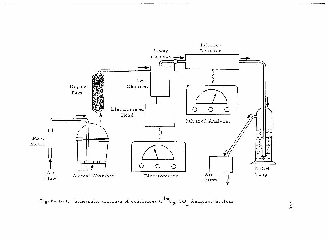
Drying Tube
Flow Meter
Air Flow
Infrared 3 -way Detector
Stopcock _0.I
Ion Chamber
,V Electrometer Head
11011.1111MIIM
Animal Chamber
O O O Electrometer
O O O
Infrared Analyzer
Air Pump
Figure B-1. Schematic diagram of continuous C 14O2/CO2 Analyzer System.
O
NaOH Trap
14
$hä 1

540
f. Vacuum pump -- equippedwith a valve to regulate air flow.
D. Experimental Procedures
1. Preparation of animals and apparatus
The flow system as illustrated in Figure B -1 should be as-
sembled and tested for constancy of air flow and freedom from leakage.
These two features are essential for the success of the experiment and
no effort should be spared in achieving them.
One should become thoroughly familiar with the operation of
the measuring instruments to be used. The instruction manuals
provided by the manufacturers should be consulted in detail in this
regard. In the case of the electrometer, this would include deter-
mining the background current in the absence of an ion chamber,
and subsequently with the chamber mounted in place and a normal
air flow passing through it. Setting the zero point and standardizing
the infrared analyzer with gas of known CO2 concentration should
also be practiced.
As the initial step in each experiment, the ion chamber back-
ground current should be measured (see Note 1 ) and the electrometer
zero point adjusted for the sensitivity range that will cover the anti-
cipated activity levels to be encountered. The infrared analyzer
should likewise be zeroed and standardized. In the case of both

541
instruments, these settings vary somewhat with time. Thus, they
must be determined anew for each experiment.
The rat to be used in each measurement period should be
fasted for 48 hours before administration of the active glucose. It
should be weighed just prior to intubation.
The glucose dose should be prepared by mixing the calculated
amount of glucose -U -C14 with 1500 mg of unlabeled glucose and dis-
solving this in sufficient water to yield a 50 percent solution (wt /vol).
This solution is then administered to the rat by means of a syringe
and stomach tube, taking care to rinse any residue from the tubing
into the stomach with a small quantity of water. The rat is imme-
diately placed in the animal chamber and the flow of air through the
system initiated.
2. The measurement period
Throughout the entire 6 -8 hour period of the experiment the
air flow must be maintained at a constant rate. This rate will have
been previously chosen, based on considerations discussed above.
Particularly in the early period of the experiment, it is
necessary to carefully observe the electrometer meter reading so
as to adjust the sensitivity range as the ion current increases to a
maximum value. The CO2 analyzer does not require such careful
1
542
attention, since total CO2 concentration should remain at a rather
constant value throughout the experiment (see Note 2).
The meter readings on both measuring instruments may be
recorded as frequently as the observer desires. Regular intervals
of 10 - 15 minutes should be often enough. If chart recorders are
available, even less attention to recording data is required. The
simplicity of such a measurement system compared to other methods
involving extensive sample preparation is evident (see Note 3).
At the end of the measurement period the animal should be
removed from the flow system and returned to its cage. It will be
necessary to place this cage under a fume hood or in a room equip-
ped with an exhaust vent for at least 24 hours to prevent C14O2 con-
tamination of the laboratory by the expired air.
An air flow should be maintained through the system until
the electrometer reading returns to the initial background level, in
order to reduce the possibility of residual contamination of the ap-
paratus.
3. Calculation and evaluation of data
The recorded electrometer meter readings (in mv) should be
converted to C14O activity in mire as follows: 2
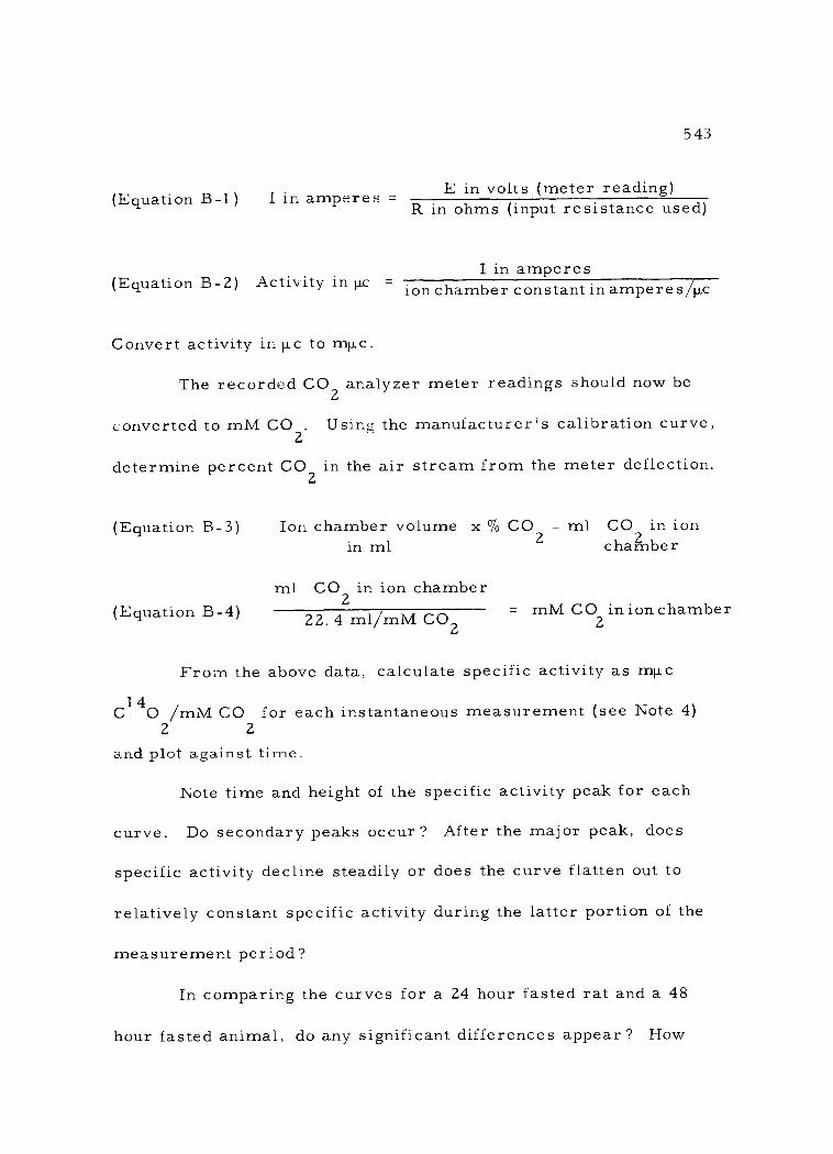
(Equation B-1)
543
I in amperes E in volts (meter reading) R in ohms (input resistance used)
(Equation B -2) Activity in µc - ion chamber constant in amperes /µc I in amperes
Convert activity in µc to mµc.
The recorded CO2 analyzer meter readings should now be
converted to mM CO2. Using the manufacturer's calibration curve,
determine percent CO2 in the air stream from the meter deflection.
(Equation B -3) Ion chamber volume x % CO = ml CO in ion in ml 2 chamber
(Equation B-4) ml CO in ion chamber
2
22. 4 m1/mM CO2 = mM CO in ion chamber
2
From the above data, calculate specific activity as mµc
C140 /mM CO for each instantaneous measurement (see Note 4) 2 2
and plot against time.
Note time and height of the specific activity peak for each
curve. Do secondary peaks occur? After the major peak, does
specific activity decline steadily or does the curve flatten out to
relatively constant specific activity during the latter portion of the
measurement period?
In comparing the curves for a 24 hour fasted rat and a 48
hour fasted animal, do any significant differences appear? How
-
2
2
544
might these be interpreted? If two or more rats have been used,
how do their respiratory CO patterns compare under the same fast - 2
ing conditions?
From the activity data calculated above, prepare a curve of
cumulative C14O recovery over the course of the experiment. Do 2
the cumulative recoveries at the end of the individual experiments
differ for the various rats and conditions used?
The data derived from this experiment can serve as a basis
for further investigations of the effects of various chemical agents
or physiological stresses on carbohydrate metabolism (1-7).
E. Experimental Notes
1. With the activity level suggested for this experiment, the
background ion current should be so small by comparison as to be
ignored. If it does appear to be considerable at any time, decon-
tamination of the ion chamber should be instituted.
2. Due to the volume of air in the flow system and mixing
factors, an initial period of up to 20 minutes may be required before
a constant CO concentration is attained. Thus, measurements of 2
CO2 concentration in the air flow prior to this time will be lower
than normal.
3. In the absence of one or both of the measuring

545
instruments, an alternative procedure may be employed. If an elec-
trometer alone is available, the total expired CO 2
may be deter-
mined by draining and replacing the solution in the NaOH trap at
brief intervals. (A pair of traps equipped with a stopcock to direct
air flow into either trap alternately is advisable. ) The absorbed
CO2 2
may then be precipitated from the solution as BaCO3 by adding
a mixture of 1 N NH4C1 and IN BaC12. From the weight of this
BaCO3, the total CO2 recovered during the sample interval may be
calculated.
If neither an electrometer or a CO 2
analyzer is available,
kinetic studies may still be carried out, although at the cost of con-
siderably more time and effort. The NaOH trap is periodically
drained as described above. However, only an aliquot of the solu-
tion is used. Planchets are prepared of the precipitated BaCO3 and
a G -M counter is employed for activity assay. Again, from the
weight of the BaCO 3
aliquot, the total CO 2
collected during the sam-
ple interval can be calculated. The cumbersome nature of such a
method contrasts sharply with the directness and relative simplicity
of the electrometer -- CO 2
analyzer system.
4. Even this calculation of specific activity can be done in-
strumentally if a ratio analyzer and recorder are employed (1 -3,
5 -6).

546
BIBLIOGRAPHY
1. Domingues, F. J. , et al. An instrument and technique for the continuous measurement of respiratory CO2 patterns in metabolic tracer studies. International Journal of Applied Radiation and Isotopes 7:77 -86. 1959.
2. Le Roy, George V. , et al. Continuous measurement of specific activity of Cl 402 in expired air. The International Journal of Applied Radiation and Isotopes 7:273 -286. 1960.
3. Tolbert, B. M. , J. H. Lawrence, and M. Calvin. Respiratory carbon -14 patterns and physiological state. In: Proceedings of the International Conference on the Peaceful Uses of Atomic Energy, Geneva, 1955. vol. 12. New York, United Nations, 1956. p. 281 -285.
4. Tolbert, B. M. , et al. Effect of coenzyme A on the metabolic oxidation of labeled fatty acids: Rate studies, instrumenta- tion and liver fractionation. Archives of Biochemistry and Biophysics 60:301 -31 9. 1956.
5. Tolbert, B. M. , Martha Kirk, and E. M. Baker. Continuous C1 402 and CO2 excretion studies in experimental animals. The American Journal of Physiology 1 85:269 -274. 1956.
6. Tolbert, Bert M. , Martha Kirk, and Frank Upham. Carbon -14 respiration pattern analyzer for clinical studies. The Re- view of Scientific Instruments 30:11 6 -1 20. 1959.
7. Wang, Chih H. , et al. Catabolism of glucose and gluconate in intact rats. Proceedings of the Society for Experimental Biology and Medicine 111 :93 -97. 1962.

547
EXPERIMENT C - THE EFFECT OF X- IRRADIATION ON BONE MARROW ACTIVITY IN RATS AS MEASURED BY IRON -59 INCORPORATION
INTO ERYTHROCYTES
The following experiment is included to exemplify a specific
use of Fe59 as a tracer in the study of erythropoiesis. It involves
tracing the fate of Fe59 ions in the albino rat as they are utilized in
hemoglobin synthesis. The actual incorporation of the Fe59 occurs
in the erythroid bone marrow, while the extent of the incorporation
is ascertained from the degree of Fe59 labeling later found in the
circulating erythrocytes after their release into the peripheral blood-
stream. Since the radionuclide used emits energetic gamma photons,
the blood cell samples are readily assayed for radioactivity by means
of a well -type NaI(T1) crystal scintillation detector.
Specifically, the experiment is designed to illustrate the use
of a radiotracer to investigate a phase of radiation biology. The
reader should not confuse the field of radiation biology, which con-
cerns the effects of radiation on living organisms, with the employ-
ment of radiotracers. The two disciplines are distinct in both pur-
pose and methodology. In this particular experiment, Fe59 incorpor-
ation is used strictly as a means to secure information on the damag-
ing effect of x- irradiation on erythropoiesis.
A. Survey of the Problem
548
The marked radiosensitivity of the hematopoietic organs has
been recognized for nearly sixty years. Penetrating radiation pro-
duces well defined changes in both the circulating blood and the blood -
forming organs. The changes observed in the circulating blood, how-
ever, appear to be due primarily to radiation effects on the hemato-
poietic tissues. The major areas of hematopoiesis are the spleen,
lymphatic tissue, thymus gland, and bone marrow. This experiment
will be concerned primarily with radiation effects on the latter tis-
sue.
The bulk of earlier information concerning the effect of radia-
tion on bone marrow was obtained by direct cytological examination
of the tissue following irradiation. After large doses (several hun-
dred roentgens) of whole -body x- irradiation, a cessation of mitotic
activity and a degeneration of hematopoietic cells is seen within less
than an hour. On the other hand, mature erythrocytes in the circu-
lating blood seemed relatively resistant to the same radiation dose.
Since these mature red cells have a rather long life span (about 120
days) little change in the red blood cell count of the circulating
blood would be noted immediately, even though all bone marrow
production were completely stopped.
549
In view of the foregoing, the use of tracer doses of Fe59
serves as a valuable method for following red cell production after
irradiation. The earliest such work was done by Hennessy and Huff
(6) at the University of California. Application of the Fe59 technique
became more feasible after the development of the NaI(Tl) crystal
scintillation detector. Over `the ensuing years the original technique
has been improved and applied to a variety of related radiobiological
problems. The list of references at the end of the experiment in-
cludes most of these significant applications and can serve as a
point of departure for further research adaptations.
The effectiveness of this technique depends on the fact that
iron is incorporated into hemoglobin molecules in red blood cells
almost entirely in the bone marrow. Only a small amount of addi-
tional iron is taken up by the red cells once they have been liberated
into the peripheral blood (8). Thus, the extent to which an injected
dose of Fe59 appears later in the circulating red blood cells is a
direct indication of activity in the bone marrow. The method is both
more sensitive and simpler than the use of cytological examination
to determine the depression of erythropoiesis in marrow tissue. As
an indication of the sensitivity of the method, Hennessy and Huff (6)
even found a detectable depression of Fe59 uptake with x -ray doses
of as low as 5 to 25 roentgens.
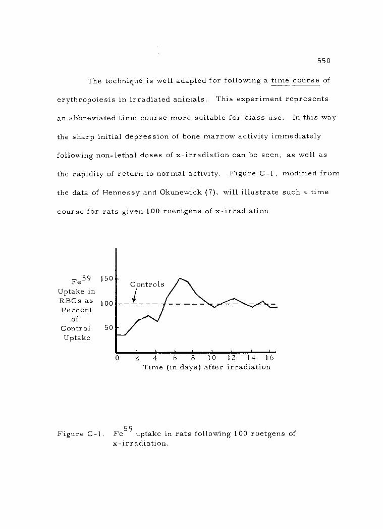
550
The technique is well adapted for following a time course of
erythropoiesis in irradiated animals. This experiment represents
an abbreviated time course more suitable for class use. In this way
the sharp initial depression of bone marrow activity immediately
following non - lethal doses of x- irradiation can be seen, as well as
the rapidity of return to normal activity. Figure C-1, modified from
the data of Hennessy and Okunewick (7), will illustrate such a time
course for rats given 100 roentgens of x- irradiation.
Fe59 150
Uptake in RBCs as 100 Percent
of Control 50 Uptake
0 2 4 6 8 10 12 14 16 Time (in days) after irradiation
Figure C-1. Fe59 uptake in rats following 100 roetgens of x- irradiation.
Controls
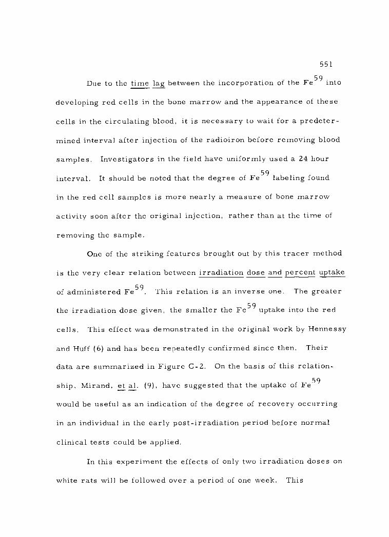
551
Due to the time lag between the incorporation of the Fe59 into
developing red cells in the bone marrow and the appearance of these
cells in the circulating blood, it is necessary to wait for a predeter-
mined interval after injection of the radioiron before removing blood
samples. Investigators in the field have uniformly used a 24 hour
interval. It should be noted that the degree of Fe59 labeling found
in the red cell samples is more nearly a measure of bone marrow
activity soon after the original injection, rather than at the time of
removing the sample.
One of the striking features brought out by this tracer method
is the very clear relation between irradiation dose and percent uptake
of administered Fe59. This relation is an inverse one. The greater
the irradiation dose given, the smaller the Fe59 uptake into the red
cells. This effect was demonstrated in the original work by Hennessy
and Huff (6) and has been repeatedly confirmed since then. Their
data are summarized in Figure C -2. On the basis of this relation-
ship, Mirand, et al. (9), have suggested that the uptake of Fe59
would be useful as an indication of the degree of recovery occurring
in an individual in the early post- irradiation period before normal
clinical tests could be applied.
In this experiment the effects of only two irradiation doses on
white rats will be followed over a period of one week. This
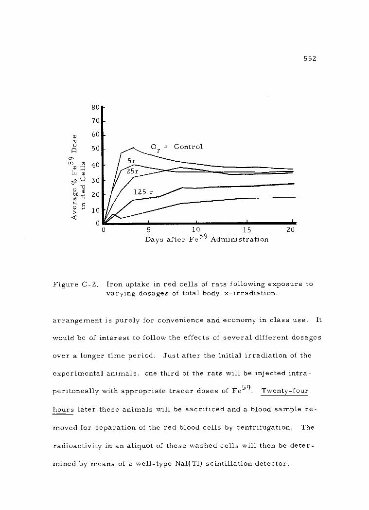
80
70
60 u) o 50
rn u) 40
Ti)
U 30 (1.)
20
a..) . 10 C
0
Or = Control
125 r
5 10 15
Days after Fe59 Administration 20
552
Figure C -2. Iron uptake in red cells of rats following exposure to varying dosages of total body x- irradiation.
arrangement is purely for convenience and economy in class use. It
would be of interest to follow the effects of several different dosages
over a longer time period. Just after the initial irradiation of the
experimental animals, one third of the rats will be injected intra-
peritoneally with appropriate tracer doses of Fe59. Twenty -four
hours later these animals will be sacrificed and a blood sample re-
moved for separation of the red blood cells by centrifugation. The
radioactivity in an aliquot of these washed cells will then be deter-
mined by means of a well -type NaI(T1) scintillation detector.
a)
`no w
b
s-i
>
553
59 Appropriate calculations of the percent of injected Fe incorporated
into the circulating red blood cells will then be made.
At three days post irradiation another one third of the rats
will be injected with Fe59 and, likewise, blood samples taken 24
hours later. Finally on the sixth day of the experiment the last one
third of the animals will be injected and their blood sampled 24 hours
later. A graphic record can then be plotted reflecting erythropoiesis
in the controls, and the two irradiated groups over the seven day
period studied.
The radioiron tracer technique has been employed as a meas-
ure of the effectiveness of radiation protective agents and therapy.
It seems admirably suited for this purpose due to its sensitivity and
relation to dose received. Bose (3) has used it to determine the pro-
tective effect of cyanide on lethally irradiated rats. Mirand, et al
(9), have employed it to measure the therapeutic effect of various
types of bone marrow transplants. This type of application of the
technique offers broad potential for further research.
B. Experimental Design
There are two basic problems to be faced in designing this
experiment. One is how much radioactivity to inject so as to get a
readily measurable amount of activity in the red cell sample. Some

554
factors to be considered are the amount of dilution occurring, the
extent of iron incorporation into red blood cells, and the well capa-
city and efficiency of the scintillation detector. The other problem
concerns the specific activity of the Fe59 to be used. The total
amount of iron injected must not be so high as to create an unphysio-
logical situation. These two issues will be taken up individually.
First, the amount of activity required must be calculated.
Since the animals given the greatest dose of radiation (the 300 r
group) will be expected to show the lowest iron uptake, the activity
required for them will be calculated. This will then be a more than
adequate amount of activity for the other two groups.
(1) Since rats average about 5 ml blood per 100 grams body
weight, if 200 gram animals are used, they can be expected to have
a total blood volume of around 10 ml.
(2) If a scintillation detector is used with a well volume of
one ml, then the activity in 1 /1 0 of the total blood volume could be
determined in a single sample.
(3) Red blood cells normally represent nearly 50% (hemato-
crit value) of the blood volume of the rat. The one ml blood sample
used could then be expected to have about 0. 5 ml of red cells, or
110 of the total red cell mass.
(4) Under the conditions of this experiment, not less than
555
five percent of the intraperitoneally injected Fe59 can be expected to
be incorporated into the circulating red blood cells. Thus, the 0. 5
ml of red cells in the counting sample would contain 0.1 x O. 05 =
0. 005 of the dose of Fe59 administered.
(5) With a scintillation well crystal having a detection effi-
ciency of about 20 percent for the 1 . 1 and 1. 3 Mev gamma rays emit-
ted by Fe59, only 0. 005 x 0. 2 = 0. 001 of the Fe59 activity would be
detected by the scintillation counter in the one ml blood cell sample.
(6) If a minimum sample count rate of at least 4, 000 cpm is
desired, then the activity injected must be 4,000/0. 001 = 4, 000, 000
dpm. This value is equivalent to just under two microcuries per
animal. Should the experimental conditions differ from those indi-
cated, appropriate adjustments following the above outline would
still allow a calculation of the amount of activity needed.
The second problem deals with the specific activity of the
Fe59 used, that is, the ratio between the activity of the radioiron
and the total amount of iron (all isotopes) in the sample. In this
particular experiment this poses no great problem. A specific acti-
vity of over 10 µc Fe59 /µg Fe is readily obtainable. The calculated
two microcurie activity above could thus be secured in less than 0. 2
micrograms of total iron. This amount is truly a tracer dose and
is well within the normal range of physiological fluctuation of this
animal.
C. Materials and Equipment Required
556
1. X -ray unit -- preferably one capable of 200 - 250 KVP output.
2. X -ray calibration instruments.
3. Well scintillation counting assembly, with supply of counting
tubes to fit the well.
4. White rats -- eighteen preferably about 200 grams and all of one
sex.
5. 36 µc Fe59C13 in citrate buffer and sterile saline -- available
from most radiopharmaceutical suppliers.
6. Compartimentalized rat irradiation chambers -- made of lucite,
wood, or wire mesh.
7. Disposable syringes (1 ml and 5 ml) and disposable hypodermic
needles (20 gauge and 26 gauge).
8. Hematocrit capillary tubes (75 mm)
9. Six cages capable of holding four rats each.
D. Experimental Procedures
1. Organization and initial irradiation
The 18 rats to be used in the experiment should be divided
into groups of six each. The six control rats will be sham
557
irradiated, while the other two groups are to be given 100 and 300
roentgens whole body x- irradiation respectively.
Immediately after irradiation two animals from each of the
three dosage groups will be injected with radioiron. Twenty -four
hours later blood samples will be taken from these animals and the
extent of radioactive labeling of their red blood cells determined.
The irradiated animals in this set will be expected to show the great-
est depression of iron uptake.
At three days post irradiation two more animals from each
dosage group will be injected and likewise their blood sampled 24
hours later. Some recovery of bone marrow activity may be seen
in the 100 r group by this time.
Finally, at six days post irradiation, the remaining animals
will be injected and sampled after a 24 hour interval. The 100 r
group should have recovered to normal or even above normal iron
uptake, while the 300 r animals may still show bone marrow depres-
sion.
The x -ray unit should be calibrated prior to the irradiation to
ensure reproducible results. Special attention should be paid to
equilization of dose over the size of field to be irradiated. It is pre-
ferable to irradiate the two groups in a compartmentalized chamber
that can hold all six animals of the group at one time.

558
The instructions that follow apply to all dosage groups during
the course of the experiment. Thus, they will not be repeated al-
though there will be three different radioiron injections and blood
sampling sequences according to the above schedule.
2. Radioiron injection
The amount of Fe59 to be used should be calculated according
to the outline described in the section on experimental design above.
Such factors as weights of the rats, detection efficiency of the scin-
tillation crystal, and size of the scintillation detector well should be
evaluated.
The total volume injected into each animal should not exceed
0. 5 ml. It should be procured or made up in a sterile saline solu-
ti on.
Proper precaution must be taken in injection to maintain
sterile conditions and to avoid introduction of an air embolus. One
syringe may be used for each set of injections if the needles are
changed between animals.
Using a 26 gauge needle with a 1 ml syringe, make an intra-
peritoneal injection into each of the six rats in the series. Care must
be taken to avoid damage to the internal organs or injection into the
intestines.
559
The precaution of wearing rubber gloves and working over a
stainless steel tray must be observed, due to the danger of spillage.
The gloves and working area should be monitored when the injections
are completed and decontamination instituted if necessary. The
syringes and needles should be immediately disposed of in the radio-
active waste container.
The two injected rats from each dosage group should be
placed in separate cages from their uninjected mates to avoid any
radioactive crosscontamination. These three cages should be ar-
ranged so that the animals' feces and urine fall through wire mesh
onto shavings and paper. Since some of the radioactive iron may be
excreted during the experiment, these wastes should be regarded as
contaminated. The cages themselves will need monitoring and pos-
sibly decontaminating at the end of the experiment.
An accurately measured aliquot of the solution used for in-
jection must be saved for later use as a relative standard. A one
percent aliquot is quite sufficient for this purpose. Place it in a
tube of the same size to be used for the blood counting sample and
dilute it to the same volume as the scintillation well capacity.
3. Removal of blood samples
Twenty -four hours after the radioiron injection, the rats
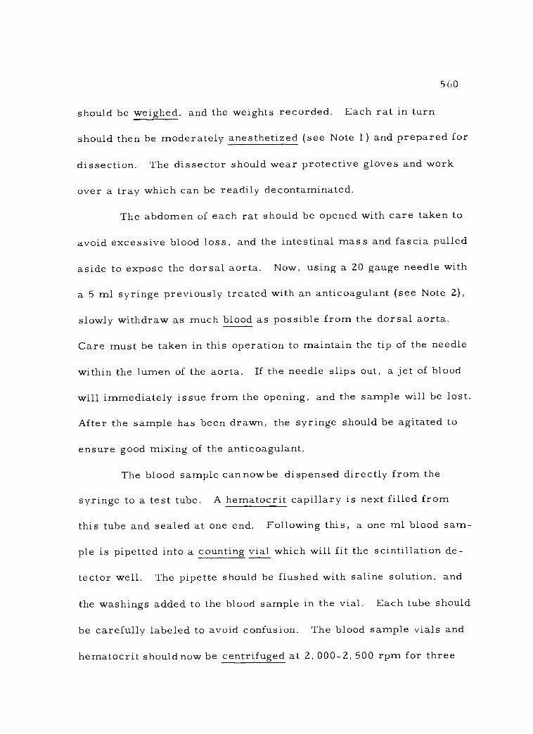
560
should be weighed, and the weights recorded. Each rat in turn
should then be moderately anesthetized (see Note 1) and prepared for
dissection. The dissector should wear protective gloves and work
over a tray which can be readily decontaminated.
The abdomen of each rat should be opened with care taken to
avoid excessive blood loss, and the intestinal mass and fascia pulled
aside to expose the dorsal aorta. Now, using a 20 gauge needle with
a 5 ml syringe previously treated with an anticoagulant (see Note 2),
slowly withdraw as much blood as possible from the dorsal aorta.
Care must be taken in this operation to maintain the tip of the needle
within the lumen of the aorta. If the needle slips out, a jet of blood
will immediately issue from the opening, and the sample will be lost.
After the sample has been drawn, the syringe should be agitated to
ensure good mixing of the anticoagulant.
The blood sample can now be dispensed directly from the
syringe to a test tube. A hematocrit capillary is next filled from
this tube and sealed at one end. Following this, a one ml blood sam-
ple is pipetted into a counting vial which will fit the scintillation de-
tector well. The pipette should be flushed with saline solution, and
the washings added to the blood sample in the vial. Each tube should
be carefully labeled to avoid confusion. The blood sample vials and
hematocrit should now be centrifuged at 2,000-2,500 rpm for three

561
minutes to separate the cells and plasma.
During this time, open the chest cavity of each rat to ensure
its death before disposing of the animal in the special "radioactive
carcass" container. All dissecting implements, cotton swabs, and
syringes that have been used should be regarded as contaminated and
treated appropriately now, too.
After centrifuging is complete, the hematocrit (the volume
percent of red blood cells in a whole blood sample) can be determined.
If a hematocrit reading device is not available, this can be done by
simple measurement using a millimeter scale.
Very carefully pipette off the clear plasma layer from the
centrifuged sample in the counting vial, avoiding any disturbance of
the packed cells at the bottom of the vial. This step and the next
are necessary to remove any traces of plasma which still contain
some of the injected Fe 59.
Add about two ml of saline solution (O. 9 %) to the cells and
centrifuge as before. Again pipette off the clear washing solution,
leaving the packed red cells ready for counting. The plasma and
this wash solution should be disposed of in the "radioactive liquid
waste" container.
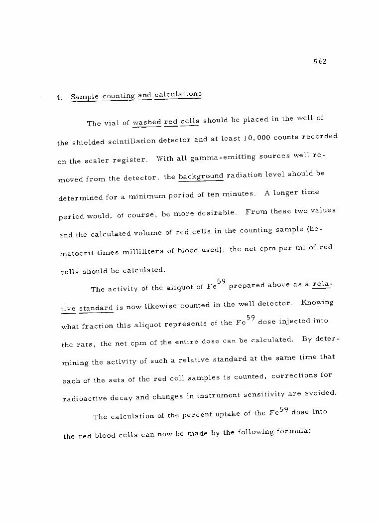
562
4. Sample counting and calculations
The vial of washed red cells should be placed in the well of
the shielded scintillation detector and at least 10,000 counts recorded
on the scaler register. With all gamma- emitting sources well re-
moved from the detector, the background radiation level should be
determined for a minimum period of ten minutes. A longer time
period would, of course, be more desirable. From these two values
and the calculated volume of red cells in the counting sample (he-
matocrit times milliliters of blood used), the net cpm per ml of red
cells should be calculated.
The activity of the aliquot of Fe59 prepared above as a rela-
tive standard is now likewise counted in the well detector. Knowing
what fraction this aliquot represents of the Fe59 dose injected into
the rats, the net cpm of the entire dose can be calculated. By deter-
mining the activity of such a relative standard at the same time that
each of the sets of the red cell samples is counted, corrections for
radioactive decay and changes in instrument sensitivity are avoided.
The calculation of the percent uptake of the Fe59 dose into
the red blood cells can now be made by the following formula:
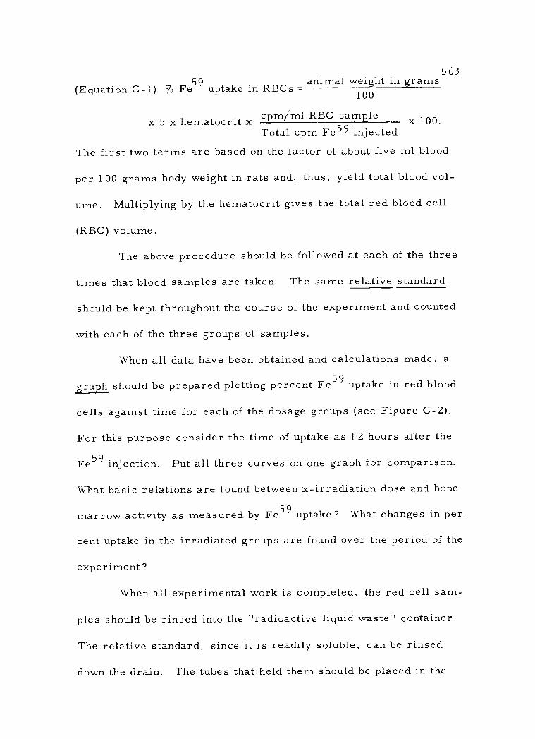
(Equation C-1) % Fe59 animal weight in grams
uptake in RBCs = 100
x 5 x hematocrit x cpm /ml RBC sample Total cpm Fe59 injected
x 100.
563
The first two terms are based on the factor of about five ml blood
per 100 grams body weight in rats and, thus, yield total blood vol-
ume. Multiplying by the hematocrit gives the total red blood cell
(RBC) volume.
The above procedure should be followed at each of the three
times that blood samples are taken. The same relative standard
should be kept throughout the course of the experiment and counted
with each of the three groups of samples.
When all data have been obtained and calculations made, a
graph should be prepared plotting percent Fe59 uptake in red blood
cells against time for each of the dosage groups (see Figure C -2).
For this purpose consider the time of uptake as 12 hours after the
Fe59 injection. Put all three curves on one graph for comparison.
What basic relations are found between x- irradiation dose and bone
marrow activity as measured by Fe59 uptake? What changes in per-
cent uptake in the irradiated groups are found over the period of the
experiment?
When all experimental work is completed, the red cell sam-
ples should be rinsed into the "radioactive liquid waste" container.
The relative standard, since it is readily soluble, can be rinsed
down the drain. The tubes that held them should be placed in the

564
container for contaminated glassware.
E. Experimental Notes
1. Etherization of the rats can be accomplished by placing a
pad of cotton sprinkled with ether in a large jar. The cotton is cov-
ered with a paper towel, the rat placed in the jar, and the jar covered.
Special precaution should be taken to avoid over -etherization. It is
necessary for the animal's heart to remain beating during blood sam-
pling, so that blood is continually pumped through the aorta. Do not
wait for complete collapse in the anesthesia chamber. Further
etherization, if necessary, can be done during dissection by placing
the rat's nose in a crucible containing a cotton pad moistened with
ether. Caution -- ether fumes are explosive. Use a well ventilated
room and ban open flames during the work.
2. Anti - coagulants may be prepared as follows: Oxalate --
pipette 0.1 ml of a 10 percent potassium oxalate solution into the
syringe to be used for blood sampling. Rotate the syringe so that
the solution covers the inner surface with a film. Place this in a
hot oven to dry as a film. Heparin -- follow a similar preparation
process, but use a solution containing O. 2 mg Heparin for every 1 . 0
ml of blood to be collected. EDTA -- similarly use a 5% solution of
sodium EDTA.

565
BIBLIOGRAPHY
1. Baxter, C. F. , et al. Anaemia and erythropoiesis in the irra- diated rat: An experimental study with particular reference to techniques involving radioactive iron. British Journal of Hematology 1 :86 -1 03. 1 955.
2. Belcher, E. H. , I. G. F. Gilbert and L. F. Lamerton. Experi- mental studies with radioactive iron. The British Journal of Radiology 27:287 -392. 1 954.
3. Bose, A. Modification of 59Fe uptake in the circulating blood of
lethally irradiated rats protected with cyanide. International Journal of Radiation Biology 4:383 -386. 1959.
4. Furth, Jacob, et al. The effect of x- irradiation on erythrogene- sis, plasma and cell volumes. Southern Medical Journal 44: 85-92. 1 951.
5. Girvin, Eb C. , and John K. Hampton, Jr. Effect of whole body x- irradiation on plasma iron turnover in rats. Proceedings of the Society for Experimental Biology and Medicine 1 00: 481 -483. 1 959.
6. Hennessy, Thomas G. and Rex L. Huff. Depression of tracer ion uptake curve in rat erythrocytes following total body x- irradiation. Proceedings of the Society for Experimental Biology and Medicine 73:436 -439. 1950.
7. Hennessy, Thomas G. and James P. Okunewick. Radioiron study of erythropoiesis after x- irradiation. 1 956. 10 p. (U. S. Atomic Energy Commission. UCLA- 383)(Microcard).
8. Lamerton, L. F. and E. H. Belcher. Effect of whole -body irradiation and various drugs on erythropoietic functions in the rat. Studies with radioactive iron. In: Advances in radiobiology: Proceedings of the Fifth International Confer- ence on Radiobiology, Stockholm, 1 955. Edinburgh, Oliver and Boyd, 1 957. p. 321 -332.

566
9. Mirand, E. A. , J. G. Hoffman and T. C. Prentice. Erythro- poietic recovery measured by Fe59 uptake in irradiated mice protected with bone marrow. Proceedings of the Society for Experimental Biology and Medicine 104:457 -461. 1960.
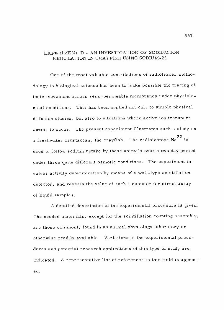
567
EXPERIMENT D - AN INVESTIGATION OF SODIUM ION REGULATION IN CRAYFISH USING SODIUM -22
One of the most valuable contributions of radiotracer metho-
dology to biological science has been to make possible the tracing of
ionic movement across semi -permeable membranes under physiolo-
gical conditions. This has been applied not only to simple physical
diffusion studies, but also to situations where active ion transport
seems to occur. The present experiment illustrates such a study on
a freshwater crustacean, the crayfish. The radioisotope Na22 is
used to follow sodium uptake by these animals over a two day period
under three quite different osmotic conditions. The experiment in-
volves activity determination by means of a well -type scintillation
detector, and reveals the value of such a detector for direct assay
of liquid samples.
A detailed description of the experimental procedure is given.
The needed materials, except for the scintillation counting assembly,
are those commonly found in an animal physiology laboratory or
otherwise readily available. Variations in the experimental proce-
dures and potential research applications of this type of study are
indicated. A representative list of references in this field is append-
ed.

A. Survey of the Problem
568
Crayfish have long been recognized as osmotically unique
crustaceans. They are able to maintain a high level of hypertonicity
in their body fluids although living in freshwater. This osmoregula-
tory ability is such that they can adjust to a wide range of salinities
with little variation in internal osmotic concentration. A prominent
feature of this ability is their ionic regulation of sodium. Blood
sodium concentrations of 200 mM /liter are not uncommon in these
animals, while the water bathing them may have a sodium concentra-
tion of only O. 4 - 2. 0 mM /liter. This situation clearly indicates one
or more sites for active transport of sodium on the animal's external
surface. Bryan (1) has identified certain cells in the gill tissues as
the most important of these sites. Since some body sodium is con-
stantly being lost by diffusion in the normal freshwater environment,
active uptake must operate more or less continually to maintain a
constant internal sodium concentration.
In order to investigate the extent and rate of this active so-
dium uptake, Na22 will be employed as a radiotracer. The rate of
Na22 uptake from a freshwater medium will be followed in three
groups of crayfish. One group will be normal animals. Their Na22
uptake will reflect the rate of active uptake necessary to replace
569
diffusional loss of sodium. A second group of animals will be greatly
depleted in body sodium by prior perfusion with distilled water for
several days. Sodium -22 uptake in this group should be much more
rapid, since the animals are replacing prior depletion of sodium as
well as correcting for continual loss by diffusion. Still a third group
of crayfish will be NaCl- loaded by prior exposure to a hypertonic
salt solution for several days. This latter group will be expected to
show a net outflux of sodium ions into the dilute freshwater until the
normal blood sodium concentration is attained. Thus, Na22 uptake
by the animals of this group should be very slight. The appearance
of any Na22 in the blood of these crayfish illustrates the dynamic
nature of ion movements through semi -permeable membranes.
In ion uptake studies of this sort, a variety of sampling tech-
niques have been employed. Bryan (1) used a clamp to hold the cray-
fish being sampled just at the water surface. He then withdrew suc-
cessive blood samples of only a few microliters from the same ani-
mal through a needle hole in its dorsal surface. In this present ex-
periment a larger blood volume is desired and this results in the
death of the animal sampled. Shaw (8) employed a circulating water
arrangement that allowed a continuous determination of activity in
the external medium. However, interval water sampling, as pre-
scribed for this experiment, should provide sufficient data to plot

570
an adequate disappearance curve.
The investigation of sodium regulation in aquatic animals,
especially marine forms, by means of radioisotopes of sodium, has
been pursued by only a comparatively few research workers. The
work of Fretter (5) and Green, et al. (6), represent typical studies
on organisms other than crayfish. In addition, regulation of other
commonly present ions has been but little explored. Bryan (4) has
further investigated cesium uptake in crabs using the radioisotope
Cs137. Chlorine -36, Ca45 and Mg28 have also been utilized in simi-
lar studies. Thus, the technique presented in this experiment has
potential for broad application in studies of ionic regulation in aquatic
animals.
B. Experimental Design
In the calculation of the amount of radioactive material to be
used in this experiment, the major concern is to have sufficient acti-
vity in the water samples so that excessively long counting times
will not be necessary. The assumptions on which these calculations
are based are in line with the references cited. The specific activity
of the Na22 poses no problem, since the sodium concentration found
in freshwater is normally in the range of 0. 4 - 2. 0 mM /i . Sodium-
22 is usually produced by the reaction Mg24(d,o()Na22, and it is thus

571
carrier free. Even a much reduced specific activity would not result
in a significant addition of sodium ions in the experimental solutions.
The amount of Na22 activity required per liter of solution can
be determined as follows:
(1) If it is assumed that the background counting rate is about
100 cpm, and that for reasonably short counting times the final five
ml water samples should show a net count rate at least ten times the
background, then a final water activity of 1, 000 cpm /5 ml is required.
(2) Assuming that, under the varied conditions of the experi-
ment, the uptake of sodium by the crayfish will deplete the solutions
by a factor of ten on the average, an initial water activity of 1 0, 000
cpm /5 ml will be needed.
(3) If the overall detection efficiency for the 1. 28 Mev gam-
ma rays from Na22 is about 25 percent in the scintillation counter
used (see Note 1), the counting rate above is equivalent to 40, 000
dpm /5 ml of solution.
(4) The activity to be introduced into each container at the
outset of the experiment would then be:
4 x 1 04 dpm 5 ml sample x 103 ml solution = 8 x 10⁶ dpm,
or just over 3. 6µc. To allow for a margin of error, it is suggested
that approximately 4 µc of Na22 be used.
572
C. Materials and Equipment Required
The following list is not exhaustive. Only those items are
listed which might not be commonly found in a physiology laboratory.
1. Crayfish: Fifteen active animals of the same species will be re-
quired. Crayfish between 10 and 20 grams are desirable. It is
preferable that all weights be as similar as possible to ensure
comparable blood volumes.
2. Shielded, well -type (5 ml capacity) NaI(T1) scintillation detector
and counting assembly.
3. A supply of counting vials to fit the scintillation detector well,
preferably a disposable type.
4. An amount of Na22C1 per container to be used as calculated ac-
cording to the above outline.
5. Containers: Plastic canisters of about 1. 5 liter capacity with
tight fitting lids will prove quite satisfactory. Two 3/8" holes
can be drilled through the lids at opposite edges. One will admit
the air line and the other will allow both air escape and water
sampling. This arrangement prevents the radioactive solution
from splashing out of the containers during aeration.
6. Distilled water: The animals to be depleted of sodium will be
perfused with distilled water for three days at a flow rate of
about one liter per hour. This will require a total flow of about
573
75 liters. It is most desirable to have a distilled water tap
available. Otherwise, a gravity flow system from a large
carboy may be arranged. It is quite important that the dis-
tilled water be cooled to room temperature before exposing
the animals to it.
7. Glass capillary tubes (3" lengths) and 5% EDTA solution: These
are used for drawing crayfish blood samples. While EDTA is
not a true anticoagulant for crayfish blood, it does slow coagula-
tion sufficiently to allow the subsequent micropipetting to be
done. Prepare the capillary tubes by filling them with the
EDTA solution and then allowing the solution to dry to a film in
them.
D. Experimental Procedures
1. Initial preparation of apparatus and animals
The fifteen crayfish are divided into three equal groups.
Each group of five animals is placed in a 2 -3 liter container parti-
ally filled with filtered pond water. If such is not available, tap
water that has been allowed to stand in an open vessel for several
days may be substituted. The water in each container should be
aerated continuously. It is advisable to observe the animals for a
day or two under these circumstances to determine their degree of
574
activity. Torpid, or obviously sick animals should be replaced.
After the observation period, the solution in one container
should be replaced with distilled water. An arrangement is now
made to circulate a flow of about 1 liter /hr of distilled water through
this container. The flow rate must be carefully adjusted. This per-
fusion with distilled water will gradually deplete the sodium ion con-
centration in the crayfish. It should be continued for three days.
Longer perfusion times or higher flow rates may lead to death of the
animals. Aeration is continued.
To the second container 300 mM NaC1 is now added per liter
of solution. This concentration is above the normal blood sodium
level (about 200 mM /liter) and will result in a gradual increase in
blood sodium concentration (see Note 2). Presumably this increase
occurs because the rate of sodium excretion cannot keep pace with
the rate of inward diffusion from the hypertonic medium. This group
of animals is left in this solution for three days under constant aera-
tion.
The crayfish in the third group will serve as controls and
will be left in the pond water under aeration while the other two
groups are being treated as described above.
Fifteen containers with tight fitting lids are now filled with
one liter each of filtered pond water. Aeration of the water must be
575
arranged, using a manifold system to evenly distribute compressed
air to individual bubblers in each container. This system can be
easily prepared from glass T- or Y- shaped connectors, rubber
tubing, and air stones. A compressed air line or pump should prove
adequate as an air supply. Provision must be made to maintain a
reasonably constant temperature. This can be accomplished by
placing the containers in a large tray through which cold water slowly
circulates.
The calculated amount of Na22C1 can now be added to each
container and thoroughly mixed with the water. Each container must
be marked to identify the animal it will hold. At the end of the three
day "conditioning" period, the crayfish may be transferred to their
respective individual containers and Na22 uptake initiated.
2. Sampling and activity determinations
The uptake of sodium by these crayfish will be followed over
the next 48 hours. This will be accomplished by determining the
22 change in Na activity in interval water samples (see Note 3) and
in crayfish blood samples secured by successive sacrifice of the
animals in each group. Details on sampling techniques are given
below. The suggested sampling schedule is as follows: Water sam-
ples should be taken from all containers with animals at 0, 2, 4, 6,
576
8, 1 6, 24, 28, 32, 40, and 48 hours after introducing the crayfish.
At 4, 8, 24, 32, and 48 hours a blood sample should be removed
from one animal in each of the three groups. This schedule is ar-
ranged for the experiment to be started in the morning so that the
most rapid activity changes may be observed during the first 1 6
hours.
Five ml water samples should be removed from each con-
tainer by pipette and placed in marked counting vials according to
the above schedule. Each vial may then be capped and placed in the
detector well directly for activity determination. This direct count-
ing of liquid samples constitutes an important advantage of the well -
type scintillation detector. After the counting operation, the con-
tents of the vials should be returned to the respective containers
from which they came. In this way a loss of activity from the solu-
tion will be avoided.
The quantity of blood removed and the manner in which it
must be taken results in the death of the crayfish involved. Prepara-
tory to drawing the blood sample, the animal is removed from its
container with rubber gloves and compressed air is blown over its
ventral side to dry off the region of puncture (see Note 4). The cray-
fish is held on its back and its legs bent dorsally along its sides. A
prepared capillary tube is then thrust through the membranous joint
577
at the basal segment of its pincer claw (cheliped) into the ventral
sinus. The animal is turned so that droplets of clear blood fall from
the end of the capillary tube onto a piece of Parafilm. It is particu-
larly important to maintain the tip of the capillary tube in the sinus
and not to probe into internal organs, such as the hepato -pancreas.
This would be evidence by the appearance of yellow- orange colored
tissue fragments in the blood (see Note 5).
When blood ceases to flow, the animal is laid aside and im-
mediately a l25µ1 sample of the blood (see Note 6) is drawn up into a
micropipette using a safety pipetter. This sample is dispensed into
a marked counting vial and two distilled water rinsings of the pipette
are added to the sample. Since the crayfish blood will commence to
coagulate in a very short time, despite the action of EDTA, these
manipulations must be done as rapidly as possible. To maintain a
comparable sample -to- detector geometry, water should be added to
the blood sample in the counting vial to bring its volume up to that of
the water samples, namely 5 ml. The crayfish is then weighed and
placed in a 30 percent solution of formalin to hasten death and pre-
vent subsequent tissue decay.
In assaying the activity of each of the water and blood sam-
ples a total of 10,000 net counts should be collected on the scintilla-
tion counter register. The calculated net activity in cpm of each
578
sample should be adjusted to net cpm /ml of blood or water.
3. Evaluation of results
From the counting data derived above, two sets of curves can
be drawn for each of the three groups of crayfish. One set will be a
plot of the activity per ml of water against time. This will show the
extent of sodium disappearance from the water with increasing time.
Since in the early hours of the experiment up to five water samples
will, be taken from each group and considerable variation within a
group may occur, average values should be plotted.
The second set of curves will be a plot of Na22 activity per
ml of blood against time. Only one value per sampling interval will
be available here, and, because of individual variations in sodium
uptake, these curves may be somewhat less than smooth.
In comparing the Na22 disappearance curves for the three
groups of crayfish, what are the significant differences between
them? Do these results seem in harmony with what might be expect-
ed, based on the initial blood sodium concentrations in the three
groups (see Note 7)? Likewise, what differences appear between the
three curves of blood Na22 activity with time? During which portion
of the experimental period does Na22 uptake proceed at the most ra-
pid rate? In view of the fact that the Natal- loaded crayfish actually
579
have a lower blood sodium concentration at the end of the experiment
than at the start, what can be inferred from the appearance of Na22
in their blood? Could this effect have been detected without the use
of radiotracer sodium?
In view of the half -life of Na22 (2. 6 yrs), decay corrections
need not be made for the activity determinations in this experiment.
The length of the half -life does, however, complicate waste disposal
procedures. The water solutions may be emptied into the drains,
since the isotope is in a soluble form and will be readily diluted.
Such cannot be done with the blood samples and carcasses. These
must be either stored in a freezer or buried at a marked disposal
site depending on local radiation safety regulations.
E. Experimental Notes
22 1. Why is Na much more suitable for this type of experi-
ment than Na 24? This latter isotope emits both an energetic beta
particle and two gamma photons per disintegration. Thus, Na
disintegration would presumably be more readily detected.
2. A variation of this procedure would be to expose some
crayfish to such a concentrated medium that had also been labeled
with Na22. After their blood sodium concentration had been thus in-
24
creased, they could be returned to normal freshwater. The outflow

580
of sodium from the blood to the solution could be followed by detect-
ing the rise in Na22 activity in the previously unlabeled water.
Bryan (3) has employed such a procedure in kinetic studies of sodium
transport.
3. A more sophisticated arrangement employs a circulating
water system, in which the solution passes through a flow -type scin-
tillation detector connected to a ratemeter (8). The change in activity
with time can thus be graphically registered on a chart recorder re-
sponding to the ratemeter signal.
4. To avoid being pinched by the claws (chelipeds) during
handling of the crayfish, it is advisable to slip short "gloves" of large
diameter rubber tubing over the pincers.
5. If time allows, it will be worthwhile to dissect the animals
and to remove samples of various organs for activity determinations.
This will reveal the internal distribution and concentration (on a per
gram wet weight basis) of sodium. It is suggested that samples
might be taken from the hepato -pancrease, muscle, exoskeleton,
gills, gut, and excretory organ (4).
6. A blood sample volume of 125 µl is chosen because this
quantity can be dependably drawn from crayfish of the size range
specified. If larger blood quantities are secured from some animals,
these may be used as counting samples with a consequent reduction
581
in the counting time required.
7. Some difficulty exists in interpreting these Na22 disappear-
ance curves. Because of the relatively small water volume to which
the animals are exposed here, the sodium concentration in the exter-
nal medium will change during the course of the experiment in the
case of the Na- depleted and the NaCl- loaded crayfish. This change
would be negligible in the natural environment of a pond or stream.
Shaw (7) attempted to correct for this by assaying the water for so-
dium by flame photometry at intervals and adjusting the sodium con-
centration accordingly.
BIBLIOGRAPHY
1. Bryan, G. W. Sodium regulation in the crayfish Astacus fluvia- tilis. I. The normal animal. The Journal of Experimental Biology 3 7:83-99. 1 960.
2. . Sodium regulation in the crayfish Astacus fluviatilis. II. Experiments with sodium -depleted animals. The Journal of Experimental Biology 37:100 -112. 1960.
3. . Sodium regulation in the crayfish Astacus fluviatilis. III. Experiments with NaCl- loaded animals. The
Journal of Experimental Biology 37:113 -128. 1960.
4. . The accumulation of radioactive caesium in crabs. Journal of the Marine Biological Association of the United Kingdom 41 :551 -575. 1 961 .
5. Fretter, Vera. Uptake of radioactive sodium (24Na) by Nereis diversicolor (Mueller) and Perinereis cultrifera (Grubs). Journal of the Marine Biological Association of the United Kingdom 34:151 -1 60. 1 955.

582
6. Green, James W. , et al. The regulation of water and salt by the fiddler crabs, Uca pugnax and Uca pugilator. The Biological Bulletin 11 6:76-87. 1 95 9.
7. Shaw, J. The absorption of sodium ions by the crayfish Astacus pallipes Lereboullet. I. The effect of external and internal sodium concentrations. The Journal of Experimental Biology 36 :126 -144. 1959.
8. . The absorption of sodium ions by the cray- fish Astacus pallipes Lereboullet. II. The effect of the ex- ternal anion. The Journal of Experimental Biology 37:534- 547. 1 960.
9. . The absorption of sodium ions by the cray- fish Astacus pallipes Lereboullet. III. The effect of other cations in the external solution. The Journal of Experimental Biology 37:548 -556. 1 960.
583
EXPERIMENT E - DETERMINATION OF COEFFICIENTS OF ZINC -65 ACCUMULATION IN FRESHWATER PLANTS
This experiment has been chosen to illustrate the use of the
gamma- emitting isotope Zn65 in following the accumulation of the
trace element zinc by various aquatic plants and algae. The experi-
mental procedure is described in detail. The experiment is design-
ed so that the activity in the plant tissue and water samples will be
detected by means of a NaI(T1) scintillation detector mounted to ac-
cept cup planchets. Other than the scintillation counting assembly,
all the materials required will be commonly found in a botanical
laboratory. Potential research applications of this study are indi-
cated and an extensive list of pertinent references is appended.
A. Survey of the Problem
It has been known for some time that many aquatic plants are
capable of accumulating certain trace elements in their tissues.
These tissue concentrations may greatly exceed those of the water in
which the plants are growing. This is in spite of the fact that such
accumulation may proceed to concentrations several orders of mag-
nitude greater than required for normal metabolism. Algae, both
marine and freshwater, have a particularly pronounced ability in
this regard.
In the present experiment this accumulative action will be

584
quantitatively determined for the element zinc by the use of the radio-
isotope Zn65. A "coefficient of accumulation" based on the uptake
of Zn65 will be determined for several species of freshwater plants
and algae. As defined by Gileva (4), this coefficient represents the
ratio between the activity detected in one gram of dry plant tissue
and the activity in one ml of the water in which the plant has been
immersed for a defined period of time under standard conditions. It
has been found that the coefficients of accumulation vary widely for
different species of aquatic plants, and for different isotopes (4,
8 -9). Since it has been reported that Zn65 uptake, in algae at least,
is markedly affected by the degree of photosynthetic activity occur-
ring (7), the variable of illumination vs. darkness will be introduced
into this experiment.
The major steps in the experiment are as follows:
(1) Selection and preparation of plant cultures and apparatus.
(2) Exposure of various plants to a defined amount of Zno5 acti-
vity in aqueous solution.
(3) Preparation and counting of plant and water samples.
(4) Calculation of coefficients of accumulation from counting
data.
Since it is desirable to have coefficients of accumulation that are
comparable from species to species, the proper selection, culturing,

585
wet weighing of the plant and algae samples are of considerable im-
portance.
The accumulative action of aquatic plants with regard to zinc
is not without practical consequence. Although a high concentration
of stable zinc in such plants does not pose a biological hazard, the
situation is altogether different when even low concentrations of ra-
dioactive Zn65 are present in rivers and coastal waters. This Zn65
will also be accumulated in the tissues of these organisms. Since
algae and other water plants are the primary food source for aquatic
animals, large amounts of Zn65 may thus enter food chains that may
end with man.
Extensive studies of this environmental hazard have been
made along the Columbia River and the inshore waters of the Oregon
and Washington coasts (2 -3, 6, 10) Since 1944, the plutonium -pro-
ducing reactors at Hanford, Washington, have added 8 - 55 curies of
Zn65 daily to the Columbia River in their cooling water effluent (1 0)
The ecological impact of this activity on the aquatic plants and ani-
mals in the river has been under continuing study by biologists at
the Hanford facility. The various environmental sampling techniques
used by these workers and the particular problem of dissemination
of this activity through food webs have been described (2 -3, 6, 10)
Davis, et al. (2) state that, "Although its abundance in the organisms
586
is less than phosphorus, sodium, or iron, the Zn65 was readily
transferred through the food web and occurred in relatively large
concentrations in almost all organisms sampled. "
Since Zn65 may be discharged in measurable concentrations
by nuclear powered ships as a corrosion product, contamination of
harbor waters may be a serious problem of the near future. The
study by Taylor (7) was part of a continuing investigation of the ac-
cumulative ability of marine algae for Zn65
Gileva (4) has investigated the possibility of exploiting the
action of algae as trace element "scavengers" for the purification of
surface waters contaminated with radionuclides. Other Soviet inves-
tigators (8 -9) have explored the action of the chelating agent EDTA
to decrease uptake of Zn65 and other radionuclides by aquatic plants,
in order to minimize the problem of radioactive material entering
natural food webs.
In most of the studies cited above, Zn65 had not been em-
ployed as a radiotracer, but has been investigated from the stand-
point of the hazard it poses in the environment. Knauss (5), how-
ever, used it and a number of other radioisotopes to study uptake of
inorganic ions, per se. Thus, the procedures employed in this ex-
periment have application both in radiotracer studies of stable iso-
tope uptake, as well as in investigation of environmental
587
contamination. Considerably more understanding of the ecological
relationships involved is needed for the development of proper waste
disposal practices in view of the increasing number of nuclear re-
actors in this country and abroad. Marine and freshwater biologists
will also find trace element accumulation studies for various organ-
isms of importance.
B. Experimental Design
In the calculation of the amount of activity to be used in this
experiment the available specific activity of Zn65 must be taken into
consideration. Specific activity is especially important in this case,
since a trace element is used. Plants generally require the element
zinc in only trace amounts. A concentration of O. 02 ppm is corn-
monly used for plant nutrient solutions. At concentrations approach-
ing 60 ppm, zinc is toxic to most plants. The concentration of zinc
found in natural surface waters varies with locale, whereas sea
water normally contains about 0. 01 ppm. The highest specific acti-
vity of Zn65 readily obtainable is about 100 me /g, or 1 /1 0 µ,g.
Thus, for each 1 µc of Zn65 activity used per liter of solution, O. 01
ppm of zinc will be added.
On the other hand, the amount of activity added to the culture
solutions must be such that a detectable quantity remains in the
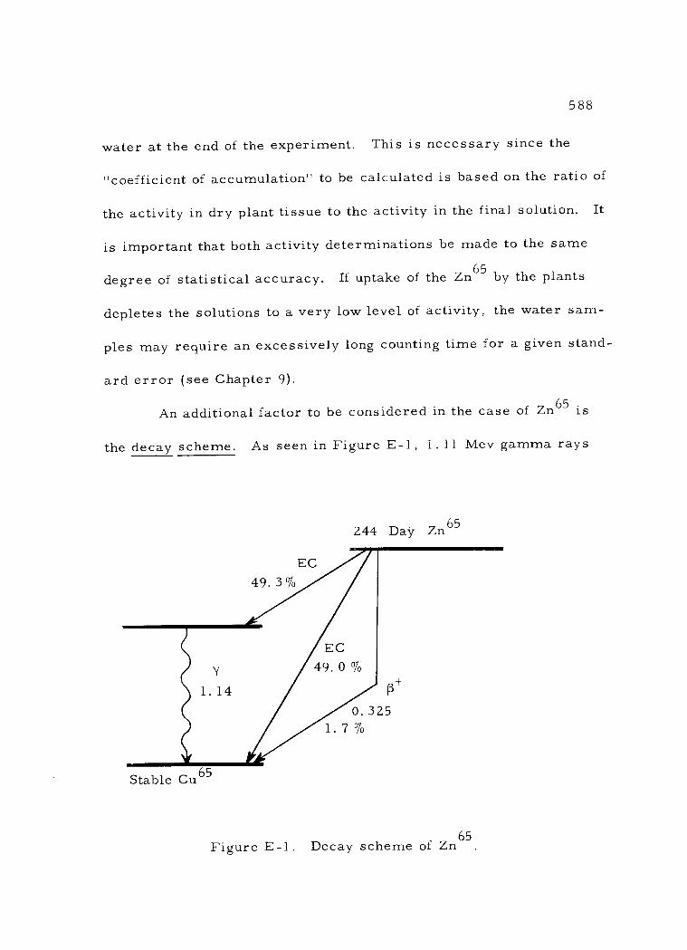
588
water at the end of the experiment. This is necessary since the
"coefficient of accumulation" to be calculated is based on the ratio of
the activity in dry plant tissue to the activity in the final solution. It
is important that both activity determinations be made to the same
degree of statistical accuracy. If uptake of the Zn65 by the plants
depletes the solutions to a very low level of activity, the water sam-
ples may require an excessively long counting time for a given stand-
ard error (see Chapter 9).
An additional factor to be considered in the case of Zn65 is
the decay scheme. As seen in Figure E-1, 1.11 Mev gamma rays
244 Day Zn65
Stable Cu65
Figure E -1. Decay scheme of Zn 65.
589
are emitted in only 49.3 percent of the radioactive disintegrations.
Since the detector to be employed is a metal encased NaI(T1) scin-
tillation crystal, only these gamma rays will be detected to any ex-
tent. The positrons and low energy x -rays resulting from electron
capture will be almost completely absorbed in the crystal housing.
Thus, only one half of the disintegrations in the sample can be de-
tected at best.
With the foregoing considerations in mind, the amount of acti-
vity needed in each 500 ml of solution can be determined as follows:
(1) If it is assumed that the background counting rate is about
100 cpm, and that for reasonably short counting times the final two
ml water samples should show a counting rate five times the back-
ground level, a final water activity of 500 cpm /2ml or 250 cpm /ml
is required.
(2) If, under the conditions of the experiment, the plant up-
take of isotope depletes the solutions by a factor of two on the aver-
age, the initial water activity would need to be approximately 500
cpm /ml.
(3) A detection efficiency of only five percent could be rea-
sonably assumed under the prescribed counting conditions (see Note
1). This would mean that an initial activity of 1 0, 000 dpm /ml , or
5 x 10⁶ dpm in the entire 500 ml of solution, would be required.
590
(4) Since only about 50 percent of the disintegrations of Zn65
yield detectable gamma radiation, on the basis of the decay scheme
above, a total nominal activity of 2(5 x 10⁶) = 1 x 10⁷ dpm would be
initially needed. This is equivalent to about 4 1/2 µc of Zn 65.
(5) At the specific activity stated above, this level of activity
would contribute 0. 9 ppm of zinc. While somewhat above normal
surface water concentrations, this should not prove toxic to the
plants used, nor is it an unrealistic level compared to concentrations
found in rivers receiving reactor effluent.
C. Materials and Equipment Required
The following list is not exhaustive, but includes only the
special materials or supplies needed for this experiment.
1. An amount of Zn65C12 of the indicated specific activity as calcu-
lated according to the above outline.
2. Plant and algae cultures: It is suggested that a minimum of four
different forms be used, including unicellular planktonic algae
(Chlorella, Chlamydomonas, or diatoms), filamentous algae
(Spirogyra, Cladophora, Ulothrix, etc. ), floating aquatic plants
(Lemna, Salvinia, Azolla, etc. ), and rooted aquatic plants
(Elodea, Cabomba, Sagittaria, etc). The specific forms chosen
will depend on local availability.

591
3. Shielded NaI (T1) scintillation detector and counting assembly.
4. Supply of cupped metal planchets to fit sample support of detector.
5. Growing containers: Plastic canisters (about one liter capacity)
with tight fitting lids are quite satisfactory. A hole can be drilled
through the lid large enough to admit the air line and allow air to
escape around it. This arrangement prevents the radioactive
solution from splashing out of the container during aeration. The
outside of containers that will hold the plants to be kept in darkness
during the experiment should be should be sprayed with black
paint.
D. Experimental Procedures
1. Initial preparation of apparatus and cultures
For each plant or algal species to be used in the experiment
prepare two containers as described in the preceding section. One
container will be placed so that it receives continuous illumination,
preferably fluorescent. The other container should be painted black
or covered with an opaque material, and placed in a dark cupboard
or closet during the time of Zn65 uptake. These containers must be
thoroughly cleaned and rinsed prior to use, since algae especially
are quite intolerant of chemical contamination.
592
Each container should be filled with 500 ml of filtered pond
water. If such is not available, tap water that has been allowed to
stand in an open vessel for several days, to allow loss of added
chlorine, may be substituted. It is important that all of the water
used be from the same source, and presumably of uniform mineral
composition. The water level should be marked on the outside of
each container, so that any evaporative losses during the experimen-
tal period may be noted, and appropriate amounts of distilled water
added.
Provision must be also made to maintain a reasonably uni-
form temperature in both experimental groups. This is readily ac-
complished by placing the containers in a large tray through which
cold water is slowly circulated.
Aeration of the culture solutions must be arranged, using a
manifold system to evenly distribute compressed air to individual
bubblers in each container. Such a system can be readily prepared
using T- or Y- shaped glass connectors, rubber tubing, and air
stones. A compressed air line or pump should prove adequate as an
air supply.
It is advisable to add the plants and algae to their respective
containers several days prior to the introduction of the radioisotope.
This procedure will allow the cultures to make an adjustment to the

593
new growing conditions before the experimental phase begins. Dur-
ing this period all containers should be illuminated and aerated.
Each plant and algal culture should be reasonably pure. Gross
contaminants in the plant cultures can be removed with forceps. It
may be necessary to rinse the algae with filtered pond water to re-
move some adhering microorganisms.
Before introducing the Zn65, the wet weight of the plant or
algal material in each container should be determined. Similar but
not identical, weights should be used. Weights of 1 0± 1 g will prove
optimal for the water volume and isotope activity specified. The
plant material may be directly weighed after excess water has been
blotted off with tissue paper. Algae, especially the unicellular
forms, will require filtration to collect the normally dispersed cells
before wet weighing is feasible.
The calculated activity of Zn65C12 solution can now be intro-
duced into each container. It should be thoroughly mixed with the
culture solution. The pH of each culture solution should also be de-
termined at this time and adjusted to within the range pH 6 -8, since
zinc solubility is considerably decreased at higher pH levels.
2. Sample preparation and counting
Two ml water samples from each container should be

594
pipetted out into marked cup planchets as soon as thorough mixing of
the activity has occurred. The plant containers are then placed in
their illuminated or darkened positions and constant aeration main-
tained. The water samples in the planchets may be slowly evaporated
to dryness under an infra -red heat lamp. The heat applied must not
be so intense as to cause boiling or loss of the sample will occur.
The activity in these initial water samples may now be deter-
mined by means of the scintillation counter. At least 10, 000 counts
should be collected from each sample and likewise for the back-
ground determination. Calculate and record results as net cpm /ml
water. How do these results compare with the amount of activity in-
troduced into the solution?
It has been found that the coefficients of accumulation stabi-
lize rather quickly (4, 8 -9). Under the conditions of this experiment
approximately four days should prove an adequate period of time for
such stabilization (see Note 2). The cultures should be inspected at
least twice daily for regulation of the aerating system, possible ad-
dition of distilled water to maintain the original level, and tempera-
ture adjustment.
At the end of the experimental period a final two ml water
sample is removed from each container. These water samples are
dried and counted as before described.
595
The plant material in each container is now harvested by fil-
tration and rinsed with tap water on the filter. The active filtrate
may be disposed of into the sink drain and flushed down with a large
quantity of water. Each plant sample should be placed in a marked,
dry, preweighed Petri dish and dried for 48 hours in an oven at 700
C. After drying, the dishes are again weighed and the net dry weight
of each sample calculated and recorded.
The dried plant samples should now be pulverized or ground
to a coarse powder. Particular caution must be observed at this
point to prevent spread of the powdered material. It is advisable to
carry out this step in a draft -free area. Marked, preweighed cup
planchets are next partially filled with this plant material. They are
reweighed and the net dry sample weight calculated and recorded.
It is advisable at this point to cover the top of each planchet
with a small piece of cellulose tape or thin plastic film (see Note 3).
This will prevent loss of material and /or contamination of the scin-
tillation detector. As an additional precaution, the samples should
be stored in covered Petri dishes,
The activity of each plant sample is now determined by means
of the scintillation counter. At least 10, 000 counts should be collect-
ed for each sample and the background radiation. Calculate and re-
cord net cpm for each sample.
596
3. Calculations and evaluation of data
Using the plant sample weights and activity determinations,
the net cpm /g dry weight for each sample may now be calculated.
This value divided by the net cpm /ml of final water samples yields
the desired coefficient of accumulation. How do these calculated
coefficients of accumulation compare with the values cited in refer-
ences 4, 8, and 9? How can any marked differences be explained?
Is there a significant difference in the coefficients of accumulation in
the continuously illuminated plants as compared to those maintained
in darkness? What conclusion concerning zinc uptake could be
drawn from this (see Note 4)?
From the activity of the initial water samples compared to
the activity of the final water samples, calculate the depletion fac-
tor resulting from plant uptake of the Zn65 (see Note 5). Based on
the counting results from the initial water samples, how many net
cpm were in each container at the start of the experiment? How do
these values compare with the measured amount of activity intro-
duced into each container?
Based on the counting results from the final water samples,
how many net cpm were in the water of each container at the conclu-
sion of the experiment? Can the difference in water activity between

597
these values and those calculated above be accounted for by the cal-
culated activity in the total plant material in each container? If not,
how might activity have been lost from these closed containers?
Similar experimental work can be done using a wide variety
of radionuclides, such as Co60, Cs137, Fe59, Rb86, etc. (8). Data
on isotope accumulation in marine algae is of particular importance,
both from the standpoint of algal physiology and inshore contamina-
tion by nuclear vessels and coastal reactors. In following up the
work cited in references 8 and 9, it would be valuable to investigate
practical methods of decreasing trace element uptake by aquatic
plants, for example, by use of chelating agents like EDTA.
E. Experimental Notes
1. A well -type scintillation detector could also be used with
an increase in detection efficiency.
2. If time allowed, it would be of interest to investigate the
extent of uptake with increasing time. Multiple containers of each
species could be prepared and each sampled at a different time. In
general, algae seem to reach their maximum uptake in a shorter
time than higher aquatic plants (4, 8).
3. What would be the effect on counting efficiency of cover-
ing a similar C14- containing sample in this way? Why can this be
598
tolerated here?
4. If time and facilities allowed, it would be of interest to
set up plant cultures under graded levels of illumination. Then it
could be determined whether zinc uptake is a direct function of de-
gree of illumination, or if there is merely an illumination threshold.
5. Why can decay of activity over the course of this experi-
ment be ignored here and in subsequent calculations?
BIBLIOGRAPHY
1. Boroughs, Howard, Walter A. Chipman and Theodore R. Rice. Laboratory experiments on the uptake, accumulation, and loss of radionuclides by marine organisms. In: The effects of atomic radiation on oceanography and fisheries. Washing- ton, 1957. p. 80 -87. (National Research Council Publication no. 551).
2. Davis, J. J. , et al. Radioactive materials in aquatic and terres- trial organisms exposed to reactor effluent water. In: Pro- ceedings of the Second United Nations International Confer- ence on the Peaceful Uses of Atomic Energy, Geneva, 1958. vol. 18. Geneva, United Nations, 1958. p. 423 -428.
3. Foster, R. F. and J. J. Davis. The accumulation of radioactive substances in aquatic forms. In: Proceedings of the Inter- national Conference on the Peaceful Uses of Atomic Energy, Geneva, 1955. vol. 13. New York, United Nations, 1956. p. 364 -367.
4. Gileva, E. A. Coefficients of radioisotope accumulation by fresh -water water plants. A Translation of the Biological Sciences Sections, Doklady, Akademii Nauk SSSR 132:343- 344. 1960.
599
5. Knauss, H. J. and J. W. Porter. The absorption of inorganic ions by Chlorella pyrenoidosa. Plant Physiology 29:229 -234. 1954.
6. Osterberg, Charles, L. D. Culm and John V. Byrne. Gamma emitters in marine sediments near the Columbia River. Science 139:916 -917. 1963.
7. Taylor, W. R. Some results of studies on the uptake of radio- active waste materials by marine and estuarine phytoplankton organisms using continuous culturing techniques. 1960. 64 p.
(U.S. Atomic Energy Commission. TID - 11783)(Microcard).
8. Timofeev - Resovskii, N. V. , et al. Coefficients of accumulation of radioactive isotopes of sixteen different elements by fresh- water organisms and the effect of EDTA on some of them. A
Translation of the Biological Sciences Sections, Doklady, Akademii Nauk SSSR 132:369 -372. 1960.
9. Timofeeva - Resovskaya, E. A. and N. V. Timofeev - Resovskii. Effect of ethylenediaminetetraacetate (EDTA) on the coeffi- cients of accumulation of different radioactive isotopes from an aqueous solution by freshwater plants. A Translation of
the Biological Sciences Sections, Doklady, Akademii Nauk SSSR 130:9 -11. 1960.
10. Watson, D. G. , J. J. Davis and W. C. Hanson. Zinc -65 in marine organisms along the Oregon and Washington coasts. Science 133:1826 -1828. 1961.

GENERAL BIBLIOGRAPHY
600
GENERAL BIBLIOGRAPHY
1. Aronoff, Sam. Techniques of radiobiochemistry. Ames, Iowa State College Press, 1956. 228 p.
2. Bleuber, Ernst and George J. Goldsmith. Experimental nucle- onics. New York, Holt, Rinehart and Winston, 1952. 393 p.
3. Broda, Engelbert. Radioactive isotopes in biochemistry. Amsterdam, Elseview, 1960. 376 p.
4. Chase, Grafton D. and Joseph L. Rabinowitz. Principles of
radioisotope methodology. 2d ed. Minneapolis, Burgess, 1 962. 372 p.
5. Comar, C. L. Radioisotopes in biology and agriculture. New York, McGraw -Hill, 1955. 481 p.
6. Cook, G. B. and J. F. Duncan. Modern radiochemical practice. Oxford, Clarendon Press, 1952. 407 p.
7. Faires, R. A. and B. H. Parks. Radioisotope laboratory tech- niques. 2d ed. London, George Newnes, 1960. 244 p.
8. Francis, G. E. , W. Mulligan and A. Warmall. Isotopic tra- cers. 2d ed. Fair Lawn, N. J. , Essential Books, 1 959. 524 p.
9. Glascock, Raymond. Labeled atoms. The use of radioactive and stable isotopes in biology and medicine. London, Sigma, 1 951. 227 p.
10. Hevesy, George. Radioactive indicators -- their applications in biochemistry, animal physiology, and pathology. New York, Interscience, 1948. 556 p.
11. Kamen, Martin D. Isotopic tracers in biology. 3d ed. New York, Academic Press, 1957. 478 p.
12. Overman, Ralph T. and Herbert M. Clark. Radioisotope tech- niques. New York, McGraw -Hill, 1960. 476 p.

601
13. Quimby, Edith H. and Sergei Feitelberg. Radioactive isotopes in medicine and biology: basic physics and instrumentation. 2d ed. Philadelphia, Lea and Febiger, 1963. 343 p,
14. Sacks, Jacob. Isotopic tracers in biochemistry and physiology. New York, McGraw -Hill, 1 953. 383 p.
1 5. Sakami, Warwick (ed. ). Handbook of isotope tracer methods. Cleveland, Dept. of Biochemistry, Western Reserve Univer- sity, 1 955. 1 88 p.
1 6. Schweitzer, Geo. K. and Ira B. Whitney. Radioactive tracer techniques. New York, D. Van Nostrand, 1949. 241 p.
1 7. Siri, William. Isotopic tracers and nuclear radiations with applications to biology and medicine. New York, McGraw - Hill, 1 949. 653 p.
18. U. S. Dept. of Commerce, National Bureau of Standards. A
manual of radioactivity procedures. Washington, 1 961. 1 59 p. (Handbook no. 80. )