Embed Size (px)
Citation preview
i
AN ABSTRACT OF THE ESSAY OF
Qammar Abbas for the degree of Master of Public Policy presented on June 10, 2019
Title: The economic effects of 2018 U.S. Steel Tariffs: An Application of Event Study
Methodology
Abstract approved:
Victor. J Tremblay
In this essay I investigate the effect of United States March 2018 steel tariffs on producers’
capital. I use intertemporal event study methodology to appraise the effect of announcement of
the tariffs on March 01, 2018 on the stock returns of major US steel companies listed at New
York Stock Exchange. I use data from Yahoo finance and include 17 US based companies in the
analysis. The results show that major steel manufacturers saw a positive shift in their returns due
to the event. Steel consumer companies included in the study showed significantly negative
returns on the event day. I include 5 US Tech firms in the control group. The event did not affect
their returns. Our evidence shows that the efficient market hypothesis holds in this case. Further,
as posited by the economic theory, the tariffs reduced overall efficiency in the market.

ii
© Copyright by Qammar Abbas
June 2019
All Rights Reserved
iii
The economic effects of 2018 U.S. Steel Tariffs: An Application of Event Study Methodology
By
Qammar Abbas
An Essay
Submitted to
Oregon State University
In partial fulfillment of
the requirements for the
degree of
Master of Public Policy
Presented June 10, 2019
Commencement June 15, 2019

iv
Master of Public Policy essay of Qammar Abbas
Victor J. Tremblay
Major Professor
Carol Tremblay
Committee Member
Elizabeth Schroeder
Committee Member
Brent S. Steel
Graduate Director, School of Public Policy, Oregon State University
I understand that my essay will become part of permanent collection of Oregon State
University. My signature below authorizes release of my essay to any reader upon
request.
Qammar Abbas
Student, Author

v
ACKNOWLEDGEMENTS
I express sincere gratitude to Professor Victor Tremblay for supervising me and
providing me timely and consistent feedback on this essay. I am grateful for his useful
instructions along the process of this study. Furthermore, I am indebted to him for answering my
questions every week in our weekly meetings with utmost patience which enriched my
understanding of economic theory. I am grateful to Professor Carol Tremblay and Professor
Elizabeth Schroeder for serving on my committee and providing my guidance and support
writing this essay.
I am extremely grateful to Professor Brent S. Steel for all his support during my Master
degree. Without his continuous support during the last two years, this journey would not have
been as rewarding as it has been.
I am thankful to Usman Siddiqi, Zehra Gardezi, Warda Ijaz and Daniyal Nadeem for their
helpful comments on an earlier draft of this essay.
I am thankful for all the support and help by my friends in the MPP 2017 cohort. I am
grateful for their friendship and all the motivation I received from every one of them. I dedicate
this essay to the memories of our good friend Rebecca Langer.
vi
TABLE OF CONTENTS
Title Page
1. Introduction………………………………………………………………………………… 1
2. Literature Review…………………………………………………………………………... 3
3. Event Study Methodology………………………………………………………………….. 6
4. Data and Analysis………………………………………………………………………….. 12
4.1 Results for Major Steel Manufacturing Companies….……………………………… 13
4.2 Results for Major Steel Consuming Firms……..…………………………………….. 18
4.3 Results for the Control Group……………………….……………………………….. 23
5. Discussion/Policy Implications……..……………………………………………………… 27
6. Conclusion………………………….………………………………………………………. 30
7. References………………………………………………………………………………….. 31
vii
LIST OF FIGURES
Figure Page
1. Abnormal Returns for 7 US Steel Manufacturing
firms for the event window………………………………………………………… 17
2. Cumulative Abnormal Returns for 7 US Manufacturing
Firms over the event window……………………………………………………….. 18
3. Abnormal Returns for 5 US Steel Consumer firms
during the event window……………………………………………………………. 22
4. Cumulative Abnormal Return of 5 US Steel Consumers
through the event window…………………………………………………………… 22
5. Abnormal returns of the 5 US Tech firms throughout
the event window……………………………………………………………………. 26
6. Cumulative abnormal returns of the 5 US Tech firms
throughout the event window………………………………………………………… 27
viii
LIST OF TABLES
Table Page
1. Summary Statistics of the Percent Change in Daily Returns for
7 US Steel Manufacturing Firms…………………………………………………………… 13
2. Regression results for 7 US Steel Manufacturing Firms…………………………………… 14
3. Abnormal Returns for 7 US Steel Manufacturing Firms…………………………………… 15
4. Cumulative Abnormal Returns for 7 US Steel Manufacturing Firms………………………. 16
5. Summary Statistics of the Percent Change in Daily Returns for
5 US Steel Consumer Firms…………………………………………………………………. 18
6. Regression results for 5 US Steel Consumer Firms…………………………………………. 19
7. Abnormal Returns for 5 US Steel Consumer Firms…………………………………………. 19
8. Cumulative Abnormal Returns for 5 US Steel Consumer Firms…………………………….. 20
9. Summary Statistics of the Percent Change in Daily Returns for 5 US Tech Firms………….. 23
10. Regression results for 5 US Tech Firms……………………………………………………. 24
11. Abnormal Returns of the 5 US Tech Firms………………………………………………….25
12. Cumulative Abnormal returns of the 5 US Tech Firms…………………………………… 26

1
The economic effects of 2018 U.S. Steel Tariffs: An Application of Event Study
Methodology
1. Introduction
On March 01, 2018 President Trump announced his intention to impose a tariff on steel
imports in the United States. A week later, on March 08 he signed an order to impose the tariff
that would become effective on March 22, 2018. The rationale for his decision was to support the
economy by giving economic relief to steel workers. He added that the tariffs would protect the
steel industry from foreign competition and protect the jobs of steel workers.
However, most economists disagree with the president’s decision. Conventional wisdom
says that a tariff, which is a tax on imports, raise the price of that commodity. This has two direct
effects. First, it raises surplus to producers of the commodity. Second, it lowers consumer
surplus. Because the gain to producers is less than the loss to consumers, a tariff makes society
worse off overall.
A tariff also has indirect or general equilibrium effects. Steel is used as a raw material in
the production of many final products, such as the construction building, automobiles, and
jetliners. Thus, a tariff on steel harms both producers and consumers in these steel using
industries.
A final concern with tariffs is that they frequently lead to trade wars. That is, country A
imposes tariffs on country B, and country B retaliates by imposing tariffs on country A. Wars
such as these stifle gains from trade and make both countries worse off.
2
Economists argue that different sectors of the economy are interrelated like different
organs in an organism. Giving protection to one area will take its toll on the other areas of the
economy. Hence, these tariffs will lead to greater losses than gains. Thus, the conventional
wisdom indicates that President Trump is wrong to think that a steel tariff is good for the U.S.
economy.
In this paper, I investigate the effects of these tariffs on the market value, reflected in
stock prices, of major steel companies. A fundamental reason for estimating the quantitative
effects of an economic policy on a market is to test whether their actual effects are consistent
with theoretical predictions. I use the inter-temporal event study methodology to determine the
economic consequences of the steel tariffs on the value of steel companies, the value of
companies that use large quantities of steel, and the value of companies that purchase little if any
steel. The contribution of this study is that it is the first to investigate the effect of the 2018 steel
tariffs on the U.S. economy.
The sample of firms includes major steel producers, steel purchasers, and firms that are
unlikely to be affected by fluctuations in steel prices. These include the 7 largest steel producers
in the U.S: Nucor Corporation, Steel Dynamics, US Steel, Carpenter Corporation, CMC Steel,
AK Steel and Allegheny Corporation. The second group includes 5 companies that are major
steel purchasers: 2 major construction firms (CAT and Cummins), 2 major automobile
producers (Ford and General Motors) and finally an aerospace company (Boeing). The third
group includes 5 major tech firms: Google, Facebook, Twitter, Amazon and Microsoft.
3
In this study, I test the predictions of the conventional wisdom. That is, the steel tariffs
should benefit steel producers, harm steel buyers, and have little or no effect on companies that
are far removed from the steel industry.
The rest of this essay is structured as follows. In the next section, I give a brief literature
review of tariff theory and event study methods. In section 3, I explain event study methodology
and my model for this study. After that, I provide the results of my analysis in section 4. In the
last section I give policy recommendations in light of this study and conclude the essay.
2. Literature Review
The event study methodology was developed by Fama et. al (1969) and Ball and Brown
(1968), and has been widely used in finance and economics. Fama et al. (1969) show how the
fundamental value of a firm, as reflected by its stock price, depends on all available information
in the market. Based on their work, the event study method implies that stock prices will
respond in a predictable way to new information that is relevant to the expected future earnings
of the firm.
Fama et al. (1969) apply their model to evaluate major stock splits of the firms at stock
exchange from 1927 to 1959. In total, they measure 940 stock splits at the New York Stock
Exchange (NYSE) in that period. The authors argue that regression of the specific returns on
market returns over time is a satisfactory method for abstracting the effect of general market
conditions on the rate of returns of individual securities. They report that residuals of the firms
show changes in the returns in anticipation of the event. Most stock splits are associated with
higher returns of the stocks around the announcement month. This effect is consistent with the
theory that stock splits will have a non-negative effect on the value of the firm. In later work

4
Fama et al. (1969) finds that the empirical evidence is consistent with the predictions of the
model.
Bhagat and Romano (2002b) review hundreds of applications of the event study
methodology. They report that most of these studies have focused on the effect of corporate law
litigations. The main objective of these applications is to determine the effect of a change in the
law on shareholders’ interests (Bhagat and Romano, 2002). However, there are fewer
applications on the effect of financial regulations.
Mackinley (1997) discusses the pitfalls that should be avoided when applying the event
study method. He also explains the assumptions on which the method is built and the proper
way to measure abnormal returns. He adds that the test of the null hypothesis assumes a normal
distribution of the returns with zero mean and standard deviation equal to one. Further,
Mackinley (1997) recommends using a 5 % significance value when testing the null hypothesis.
Moreover, he adds that the power of the event studies can be increased by using a larger sample
size by including more companies in the sample by shortening the pre-event window. Pre-event
window is the duration in the event window before the event day t and post-event window is the
duration after the event day t. To get more accurate results, Bhagat and Romano (2002a)
recommended taking a longer estimation window. Mackinley (1997) advises to take shorter time
intervals preferring daily returns to weekly or monthly stock returns. Lastly, he recommends
taking an event window rather than an event day to account for any information leaks in the
market (MacKinlay, 1997).
Jarrell (1985) uses the event study methodology to investigate the deregulation of
Securities Exchange Commission Act (SEC). The act regulated brokerage rates on exchanges on
5
the New York Stock Exchange with rates that are market determined. Jarrell was one of the first
to use this method to evaluate the economic effect of government regulation/deregulation. He
reported that the deregulation increased the returns of the top 25 brokerage firms. Further, it
decreased the returns of the SEC and the underwriting firms (Jarrell, 1984).
Gokhale et. al. (2014) use the event study method to measure the effects of several
product recalls on Toyota automobiles, due to braking concerns, on stake holders’ wealth. The
authors report that the minor recall had no significant effect on Toyota returns while a later major
recall reduced Toyota returns significantly. The authors argue that the difference in the effect of
the event on returns shows that investors put high value on information deriving from unbiased
experts. The major recall had a significant negative impact on company value, indicating
consumer concerns with Toyota’s technical ability and future profit. This is consistent with the
predictions of the efficient market hypothesis. Lastly, third party verification of Toyota’s braking
reliability on which the major recall was based had a significant positive impact on Toyota
returns, implying that investors had confidence in Toyota’s future profitability.
Due to its elegant simplicity, the event method has been applied in other disciplines such
as law, management, marketing, history and political science. Event studies provide a good
opportunity to observe changes in the stock values at the stock market which can be a good tool
to measure the short term effects of corporate litigation (Corrado, 2011). It has been used to
measure the effects of auto industry product recalls by Jarrell and Peltzman (1985) and by
Thomsen and McKenzie (2001) to examine food industry recalls. It has been used to measure the
effects of corporate litigation on stock holders’ wealth by Jahera and Pugh (1991) and Romano
(1990).
6
Cornell and Morgan (1990) provide an overview of the strengths and weaknesses of the
event study methodology for analyzing impact of regulations. They argue that if an adequate
sample of the firms from the same industry facing regulation is not selected, the methodology
will result in overestimating or underestimating the effects of regulations. They add that if
information about the implementation of a regulation is leaked before the announcement date,
the methodology will underestimate the effect of the event on the event day. They recommend
taking a longer event period in order to capture the impact of the information that are available to
the public. The authors add that this method may fail when the exact event date is unclear. In
order to capture the true impact of the event on stock returns, it is imperative that the event dates
are accurate (Cornell and Morgan, 1990).
In the next section, I describe the model, event method, and the significance test being
used in detail.
3. Event Study Methodology
I use the event method to analyze the effect of new tariffs on major steel firms’ stock
returns. This method was developed by Fama et al. (1969), and Bhagat and Romano (2002)
review the methodology and its various applications to finance and economic policy issues.
Event study analysis is one of the most successful uses of econometrics in policy analysis. By
providing an anchor for measuring the impact of events on investor wealth, the methodology
offers a fruitful means for evaluating the welfare implications of private and government actions.
The event study method is based on the market model of stock valuation. It assumes that
the price of a stock reflects the time and risk adjusted discounted present value of all future cash
flows that are expected to accrue to the holder of that stock. According to the semi strong version
7
of the efficient market hypothesis, the price of a stock reflects all publicly available information
in an unbiased manner. Because the price of a stock reflects this information at any point in time,
it is impossible for the average investor to earn abnormal returns (i.e., an economic profit) by
investing in the stock market.
In particular, the return on i at time t (Rit) is a function of all available market
information, which is measured as the market return on a large portfolios of stocks (Rmt). The
market model assumes a stable linear relationship:
𝑅𝑖𝑡 = 𝛼𝑖 + 𝛽𝑖𝑅𝑚𝑡 + 𝜀𝑖𝑡, (1)
𝜀𝑖𝑡 ~ 𝑁(0, 𝜎2),
where the error term 𝜀𝑖𝑡 depends on unanticipated random events and is purely white
noise.
Therefore, only an unanticipated event can change the price of a stock. This change
should reflect the expected changes in the future cash flows of the firm or in the riskiness of
these cash flows. Thus, an event that impacts the financial performance of a firm will experience
an abnormal movement in the price of the stock. Movements in the stock market overall are
usually subtracted from the stock’s price movement in estimating the abnormal return.
Our goal is to test the null hypothesis that an event such as an announcement of a tariff
has no effect on a company’s abnormal returns. An abnormal return is defined as the actual ex
post return minus the expected return. The normal return equals the expected return, conditional
on the event never taking place. Formally, the abnormal return for firm i at event date τ is
AR𝑖𝜏 = R𝑖𝜏 − E(R𝑖𝜏|R𝑚𝜏), (2)
8
where E(R𝑖𝜏|R𝑚𝜏) is the expected normal return and R𝑚𝜏 is the pre-event conditioning
information for the normal return model. In other words, R𝑚𝜏 is the information that is used to
forecast the expected return assuming that the event never happens.
An event study has four components: defining the event and announcement day,
measuring the stock’s return during the announcement period, estimating the expected return of
the stock during this announcement period in the absence of the announcement, and computing
the abnormal return (actual return minus expected return) and determining its statistical and
economic significance.
Events under investigation are usually the announcements of various corporate, legal, or
regulatory action or proposed action. After defining the event, the researcher searches for the
first public announcement of the event. This is crucial because under the semi strong form of the
efficient market hypothesis, the impact of the event on the value of the firm would occur when
information about the event becomes public (i.e., on the announcement date). In our study the
event is the imposition of steel tariffs by President Trump in March 2018. Our event date is
March 01, 2018 when the President announced that 25% tariff would be imposed on all steel
imports. On March 8th, he signed the order and the tariff went into effect on the 23rd of March,
two weeks after he signed the orders.
To successfully implement this method requires stock price (and dividend) data before
and after the event date. Let τ = 0 be the event date and Wpre be the pre-event time period or
estimation window. Let Tpre be the number of observations (days) in Wpre. The event window
(Wevent) identifies the time it takes for the event information to fully affect returns. In a perfectly
efficient financial market, this will be a very short length of time and would include just one time
9
period. With real world imperfections, however, there may be information leaks before the event
and lags in response to the event. With information leaks, Wevent starts before τ = 0; if it takes
time for investors to evaluate the economic consequences of an event, then Wevent extends into
several periods after τ = 0.
In this study, the event day is March 01, 2018. I use a five day period before the
announcement to account for information leaks and 10 days after the event to account for any
other unanticipated disturbance in the market. The event window in this study is 16 business
days (-5 days before t=0 event day = 0, +10 after event day t=0) starting from February 23, 2018
and extends through March 15, 2018.
After defining the event and announcement period, one measures stock returns for this
period. If daily returns are being used, this is straightforward: the return is measured through
closing prices. In this study I use percentage stock returns of the firms listed on New York Stock
Exchange.
The next step is to estimate the expected return of the stock during the announcement
period assuming that the event never took place. Although it is straightforward to measure the
actual return for the announcement period, determination of the impact of the event itself on the
share price is more difficult. To measure this impact, the expected return must be subtracted
from the actual announcement period return. The expected return is the return that would have
accrued to the shareholders in the absence of this or any other unusual event.
It is customary for researchers to use between 100 and 250 daily returns preceding the
announcement period. I use a 246 days estimation window in this study. A longer window will
lead to a more precise estimate; however, a longer window increases the likelihood that it
10
contains information caused by other events (Bhagat and Romano 2002). The unexpected event
period return, also known as the abnormal returns are defined as the actual returns observed in
the market minus the estimated expected return during the event period.
The next step in evaluating the financial effect of an event is to accurately estimate
expected normal returns. This requires estimation of the market model in equation 1. Under the
conditions of the model, the parameters can be estimated with data from Wpre using ordinary
least squares (OLS). Parameter estimates (αi and βi) and market data from Wevent are used to
forecast normal returns during the event window(R𝑖𝜏|R𝑚𝜏). Thus, the abnormal return at time τ
is
AR𝑖𝜏 = R𝑖𝜏 − E(R𝑖𝜏|R𝑚𝜏). (3)
For the classic market model,
AR𝑖𝜏 = R𝑖𝜏 − (αi + βiR𝑚𝜏). (4)
When Wevent includes more than one period, sample abnormal returns are added up to obtain
cumulative abnormal return, CAR𝑖𝜏. If Wevent ranges from τ = τ1 < 0 to τ = τ2 > 0, then
CAR𝑖𝜏 = ∑ AR𝑖𝜏𝜏2𝜏=𝜏1
. (5)
This measures the total effect on abnormal returns for a multi-period event window. If the
event has no effect on the value of the firm, then ARiτ (and CAR𝑖𝜏) will not be significantly
different from zero, because actual returns will not significantly differ from normal returns. For a
positive (negative) event, however, both AR𝑖𝜏 and CAR𝑖𝜏 will be positive (negative) and
significantly different from zero.

11
The final step is to compute the statistical significance of this abnormal return. The
standard error of the residuals from the estimated statistical model can be used as an estimate of
the standard error for the announcement period abnormal return. However since individual
stocks are quite volatile, this standard error could be quite high relative to the abnormal return.
Event studies usually consider a sample of firms that have made or been the subject of the same
type of announcement. One benefit of this approach is that it increases the likelihood that no
other information besides the event under study will be valued since any additional unexpected
information disclosed on one firm’s announcement date will wash out with that on other firms’
announcement days.
Traditional parametric tests have been discussed in Serra (2004) and Bhagat and Romano
(2002). These tests generally assume that ARit is independently and identically distributed with
mean zero and variance (ARit). In this case,
σ2(AR𝑖𝑡) = σ2 (1 +1
Tpre+
(R𝑚𝑡−R𝑚)2
∑ (R𝑚𝜏−R𝑚)2𝜏∈Wpre
) (6)
where R𝑚 is the mean of market returns over the estimation window. We assume that the event
has an effect on the mean and not the variance of abnormal returns during the event window. We
can use the distributional properties of abnormal returns to make statistical inferences on
abnormal returns for the event window. The null hypothesis is that abnormal returns are not
different from zero during the event window. In order to compute the test statistic for abnormal
returns, we standardize each daily abnormal return
SAR𝑖𝜏 = AR𝑖𝜏 σ(AR𝑖𝑡)⁄ . (7)
SAR𝑖𝜏 follows a t-distribution with Tpre-2 degrees of freedom.
12
CARit is assumed to be distributed independently and identically with mean zero and
variance σ2(CAR𝑖𝑡). The variance of CAR on day τ is given by the following expression
σ2(CAR𝑖𝑡) = σ2 (k +k2
Tpre+
∑ R𝑚𝜏τ2τ1
−k(R𝑚)2
∑ (R𝑚𝜏−R𝑚)2τ∈Wpre
), (8)
where parameter k is the day within the event window. The null hypothesis is that each
cumulative abnormal return is not different from zero. The test statistic that is used to test the
null hypothesis above is given by the following expression for standardized cumulative abnormal
returns (SCAR)
SCAR𝑖𝜏 = CAR𝑖𝜏 σ(CAR𝑖𝑡)⁄ (9)
Under the null hypothesis of no abnormal performance, the Test statistic has a student-t
distribution with t-d degrees of freedom.
4. Data and Analysis
The raw data include adjusted closing prices of daily stocks of the firms included in the
study and the market index measured as the Standard and Poor 500 Index (S&P 500). These data
are obtained from Yahoo Finance. Daily returns of the firms are the daily percentage change in
the firm’s stock closing price and S&P returns is the daily percentage change in the value of S&P
500 Index.
In this study, seventeen firms are analyzed. In the first group, I include seven major US
steel manufacturing firms. They are Nucor Corp., US Steel Corporation, Steel Dynamics, CMC
Steel, Carpenter Steel, Allegheny Steel and AK Steel Company. In the second group, I calculate
abnormal returns for 5 major consumers of steel. They include two major construction firms
13
(Caterpillar and Cummins), a major aircraft producer (Boeing) and two major automobile
manufacturers (Ford and General Motors). In the third and final group I analyze the returns of 5
major tech companies: Amazon, Twitter, Facebook, Google and Microsoft. Economic theory
predicts that the event will: (1) cause the major steel manufacturers to have significantly positive
returns on the event day, (2) cause major steel consumers to have negative returns, and (3) have
no effect on the returns of the control group that has no direct link to the steel industry.
I use 246 days estimation window for all the firms included in the study. The estimation
window starts at March 01, 2017 and ends at February 22, 2018. For all the firms, the event
window is 16 days. Event date for this study is March 01, 2018 when President Trump made the
announcement. The event window starts 5 days before the event to account for the leak of
information and ends 10 days after the event to capture its full effect. Thus, event window starts
at February 23, 2018 and ends at March 15, 2018.
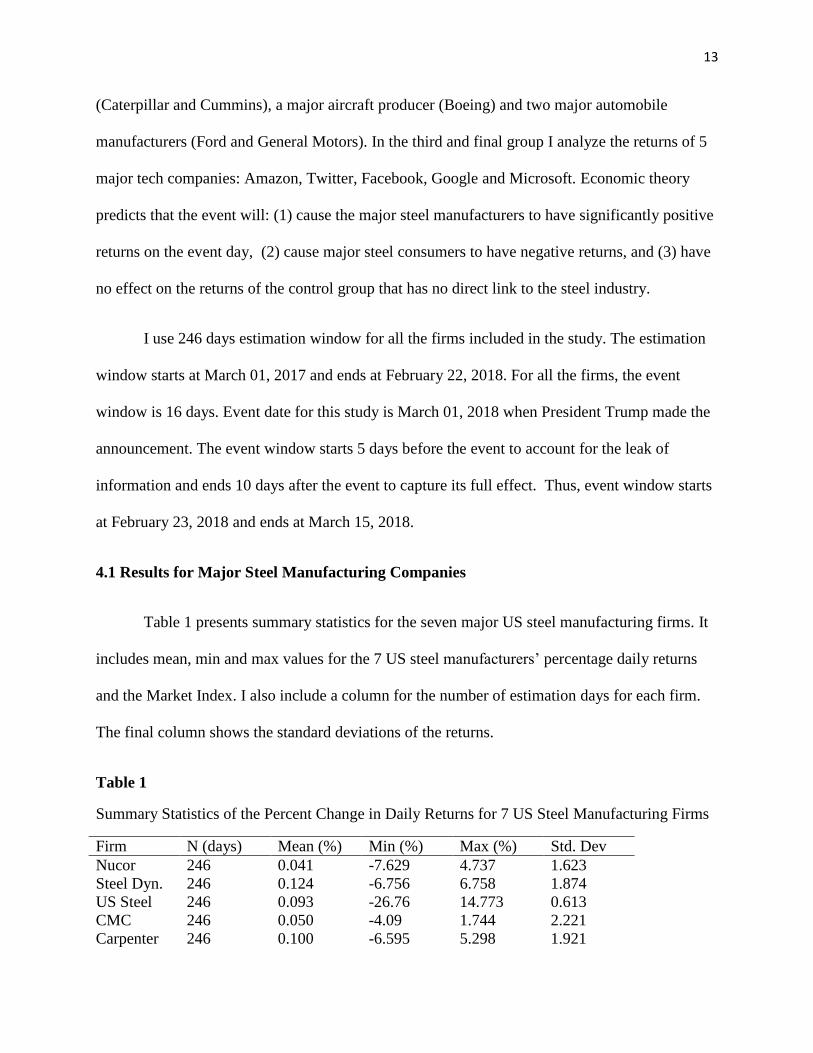
4.1 Results for Major Steel Manufacturing Companies
Table 1 presents summary statistics for the seven major US steel manufacturing firms. It
includes mean, min and max values for the 7 US steel manufacturers’ percentage daily returns
and the Market Index. I also include a column for the number of estimation days for each firm.
The final column shows the standard deviations of the returns.
Table 1
Summary Statistics of the Percent Change in Daily Returns for 7 US Steel Manufacturing Firms
Firm N (days) Mean (%) Min (%) Max (%) Std. Dev
Nucor 246 0.041 -7.629 4.737 1.623
Steel Dyn. 246 0.124 -6.756 6.758 1.874
US Steel 246 0.093 -26.76 14.773 0.613
CMC 246 0.050 -4.09 1.744 2.221
Carpenter 246 0.100 -6.595 5.298 1.921
14
Allegheny 246 0.160 -7.827 11.493 2.729
AK Steel 246 -0.101 -21.538 13.740 3.774
S&P 500 246 0.050 -4.097 1.744 0.613
Table 2 presents the OLS parameter estimates from the market model for the 7 steel
Firms listed in Table 1. The table shows that there is a significantly positive association between
6 major companies’ returns and market returns. Returns for Carpenter Corporation and
Allegheny Steel are not significant. Parameter estimates from each model are used to generate
estimates of the abnormal returns and of cumulative abnormal returns for the event day, 5 trading
days prior and 10 trading days after the event.
Table 2
Regression results for 7 US Steel Manufacturing Firms
Variable Steel
Dynamics
Carpenter AK Steel Allegheny CMC US Steel Nucor
Intercept(αi) 0.057 0.023 -0.188 0.041 0.025 0.012 -0.02
N 246 246 246 246 246 246 246
R2 0.18 0.23 0.07 0.20 0.15 0.11 0.26
Slope(𝛽𝑖) 1.31*
1.53* 1.71* 1.95 2.04* 3.14* 1.36*
Std. Error (1.69) (1.68) (3.63) (2.32) (2.04) (3.14) (1.39)
Standard errors in parentheses. * p<0.05
Table 3 presents the percentage abnormal returns for the 7 steel companies for each event
window. To test the null hypothesis that the event had no significant impact on the returns of the
firms, I conduct parametric test. T-values are given in parentheses for each day of the window.
For 5 of the major companies namely Nucor corporation, Steel Dynamics, US Steel, CMC
Corporation and AK Steel the returns are significantly different from zero at 5% level. All of
these firms showed positive returns on the event day. For Carpenter Corporation and Allegheny
Steel the returns on the event day are not significantly different from zero. Nucor Corporation
15
saw 5.1% increase in their returns while Steel Dynamics saw 5.7% increase in their returns. AK
Steel gained the highest increase in their returns at11.9%. US Steel saw 8.2 % increase in their
returns while CMC Corp. returns increased by 6.8%. None of the companies saw any significant
increase before the event date which suggests that there was no appreciable leak before the event.
Nucor, US Steel and Steel Dynamics report negative returns on 5 day of the event when
President Trump signed the orders on 8th March, 2018.
Table 3
Abnormal Returns for 7 US Steel Manufacturing Firms
Event day Nucor Steel Dyn US Steel CMC Carpenter Allegheny AK Steel
-5 0.044
(0.031)
-0.476***
(-0.281)
0.086
(0.027) *
-1.784
(-0.872)
0.223
(0.132)
2.587
(1.112)
-1.208
(-0.332)
-4 -2.179
(-1.564)
-3.275*
(-1.932)
-1.732
(-0.551)
-0.458**
(-0.224)
-1.707
(-1.015)
-0.801
(-0.344)
-4.692
(-1.291)
-3 -0.175
(-0.126)
-0.449
(-0.265)
-0.242
(-0.077)
-0.752
(-0.367)
-0.160
(-0.095)
-3.3324
(-1.429)
0.901
(0.248)
-2 0.896
(0.643)
0.555
(0.327)
1.512
(0.481)
0.142
(0.069)
1.171
(0.696)
2.585
(1.111)
-0.820
(-0.225)
-1 -1.263
(-0.906)
-1.246
(-0.735)
0.933
(0.297)
-1.901
(-0.929)
0.367
(0.224)
-2.020
(-0.868)
-3.577
(-0.984)
0 5.107***
(3.666)
5.699***
(3.363)
8.206***
(2.611)
6.851***
(3.349)
2.663
(1.584)
1.400
(0.602)
11.967***
(3.294)
1 -0.147
(-0.105)
-0.248
(-0.146)
-2.301
(-0.732)
1.056
(0.516)
-2.632
(-1.566)
2.796
(1.202)
0.027
(0.007)
2 -1.510
(-1.084)
-3.622***
(-2.138)
-3.470
(-1.104)
-2.519
(-1.231)
-1.254
(-0.746)
-0.651
(-0.280)
-3.634
(-1.000)
3 -0.450
(-0.323)
-1.124
(-0.663)
-0.994
(-0.316)
-0.750
(-0.366)
0.858
(0.510)
2.073
(0.891)
0.453
(0.124)
4 2.602*
(1.867)
0.772
(0.455)
2.681
(0.853)
1.954
(0.955)
0.929
(0.553)
0.305
(0.131)
1.339
(0.368)
5 -3.245***
(-2.329)
-3.456***
(-2.039)
-3.774
(-1.200)
-4.219**
(-2.062)
-2.022
(-1.203)
1.631
(-0.701)
-4.625
(-1.273)
6 -3.043**
(-2.184)
-1.609
(-0.950)
-4.727
(-1.504)
-1.904
(-0.930)
-1.211
(-0.720)
-1.038
(-0.446)
-6.274
(-1.727)
7 0.991
(0.711)
1.491
(0.880)
-0.050
(-0.016)
1.103
(0.539)
1.273
(0.757)
1.482
(0.637)
2.308
(0.635)
8 0.662
(0.475)
1.334
(0.787)
-6.474**
(-2.060)
-0.017
(-0.008)
0.300
(0.178)
-0.722
(-0.310)
-1.892
(-0.520)
9 -1.454 0.337 -3.572 -2.482 -2.361 -0.707 -5.188
16
(-1.044) (0.199) (-1.136) (-1.213) (-1.404) (-0.304) (-1.428)
10 0.407
(0.292)
-1.314
(-0.775)
0.262
(0.083)
-0.810
(-0.396)
-1.852
(-1.101)
-1.812
(-0.777)
1.762
(0.485)
t-statistics in parentheses. * p<0.1, * *p<0.05, *** p<0.01
Table 4
Cumulative Abnormal Returns for 7 US Steel Manufacturing Firms
Event
day
Nucor Steel
Dyn
US Steel CMC Carpenter Allegheny AK Steel
-5 0.044
(0.031)
-0.476
(-0.281)
0.086
(0.027)
-1.784
(-0.872)
0.223
(0.132)
2.587
(1.112)
-1.208
(-0.332)
-4 -2.134
(-1.532)
-3.751**
(-2.214)
-1.645
(-0.523)
-2.243
(-1.096)
-1.483
(-0.882)
1.785
(0.767)
-5.900
(-1.624)
-3 -2.310
(-1.658)
-4.201**
(-2.479)
-1.888
(-0.600)
-2.995
(-1.464)
-1.643
(-0.978)
-1.539
(-0.662)
-4.999
(-1.376)
-2 -1.413
(-1.014)
-3.645***
(-2.151)
-0.375
(-0.119)
-2.852
(-1.394)
-0.472
(-0.281)
1.046
(0.449)
-5.819
(-1.601)
-1 -2.676*
(-1.921)
-4.892***
(-2.887)
0.557
(0.177)
-4.754**
(-2.324)
-0.096
(-0.057)
-0.974
(-0.418)
-9.397**
(-2.586)
0 2.430
(1.744)
0.806
(0.476)
8.764***
(2.788)
2.097
(1.025)
2.567
(1.527)
0.426
(0.183)
2.570
(0.707)
1 2.283
(1.638)
0.558
(0.329)
6.462**
(2.056)
3.153
(1.541)
-0.065
(-0.038)
3.222
(1.385)
2.598
(0.715)
2 0.772
(0.554)
-3.064
(-1.808)
2.991
(0.951)
0.633
(0.309)
-1.319
(-0.784)
2.571
(1.105)
-1.036
(-0.285)
3 0.321
(0.231)
-4.188**
(-2.472)
1.997
(0.635)
-0.117
(-0.057)
-0.460
(-0.273)
4.644
(1.997)
-0.582
(-0.160)
4 2.924**
(2.099)
-3.415**
(-2.016)
4.679
(1.488)
1.837
(0.898)
0.469
(0.279)
4.950**
(2.128)
0.756
(0.208)
5 -0.320
(-0.230)
-6.872*
(-4.056)
0.905
(0.287)
-2.381
(-1.164)
-1.552
(-0.923)
3.318
(1.427)
-3.868
(-1.064)
6 -3.364**
(-2.415)
-8.481***
(-5.006)
-3.822
(-1.216)
-4.285**
(-2.094)
-2.764
(-1.644)
2.280
(0.980)
-10.143**
(-2.792)
7 -2.373
(-1.703)
-6.990***
(-4.125)
-3.873
(-1.232)
-3.182
(-1.555)
-1.490
(-0.886)
3.763
(1.618)
-7.835**
(-2.156)
8 -1.711
(-1.228)
-5.655***
(-3.338)
-10.347**
(-3.292)
-3.200
(-1.564)
-1.189
(-0.707)
3.040
(1.307)
-9.728**
(-2.677)
9 -3.165***
(-2.272)
-5.318***
(3.139)
-13.919**
(-4.429)
-5.683**
(-2.778)
-3.550**
(-2.112)
2.333
(1.003)
-14.917**
(-4.106)
10 -2.758**
(-1.979)
-6.633**
(-3.914)
-13.657**
(-4.345)
-6.493**
(-3.174)
-5.402**
(-3.214)
0.520
(0.223)
-13.154**
(-3.620)
t-statistics in parentheses. * p<0.1, * *p<0.05, *** p<0.01
17
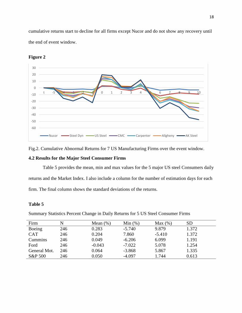
Table 4 presents percentage cumulative abnormal returns for the 7 steel firms. Among the
7 firms only US Steel’s returns are significantly positive on the event day and the day after.
Nucor and Allegheny report significantly positive returns on the 4th day. Nucor loses the market
on the 6th and 9th day of the event. Steel Dynamics show significantly negative returns starting
from 3rd day of the event till the 10th day. US Steel, CMC and AK Steel shows significantly
negative returns on the last 3 days of the event window.
Figure 1 shows abnormal returns for the 7 US steel manufacturing firms. The figure
shows that most firms saw an increase in the returns on the event day. AK Steel saw the highest
increase in their returns followed by Steel Dynamics and US Steel. Nucor saw a steady increase
in their returns. Further, the figure shows that most firms included in this group returned to their
pre-event level at by the end of event window.
Figure 1
Fig.1. Abnormal Returns for 7 US Steel Manufacturing firms for the event window.
Figure 2 shows cumulative abnormal returns for the 7 US steel Manufacturing firms. The
figure shows an increase in cumulative returns for most firms in the first two days of the event.
The cumulative returns show a stable trend over the next three days. By the 5th day of event, the
-40
-20
0
20
40
60
T -5 -4 -3 -2 -1 0 1 2 3 4 5 6 7 8 9 10
Nucor Steel Dyn US Steel CMC Carpenter Allgheny AK Steel
18
cumulative returns start to decline for all firms except Nucor and do not show any recovery until
the end of event window.
Figure 2
Fig.2. Cumulative Abnormal Returns for 7 US Manufacturing Firms over the event window.
4.2 Results for the Major Steel Consumer Firms
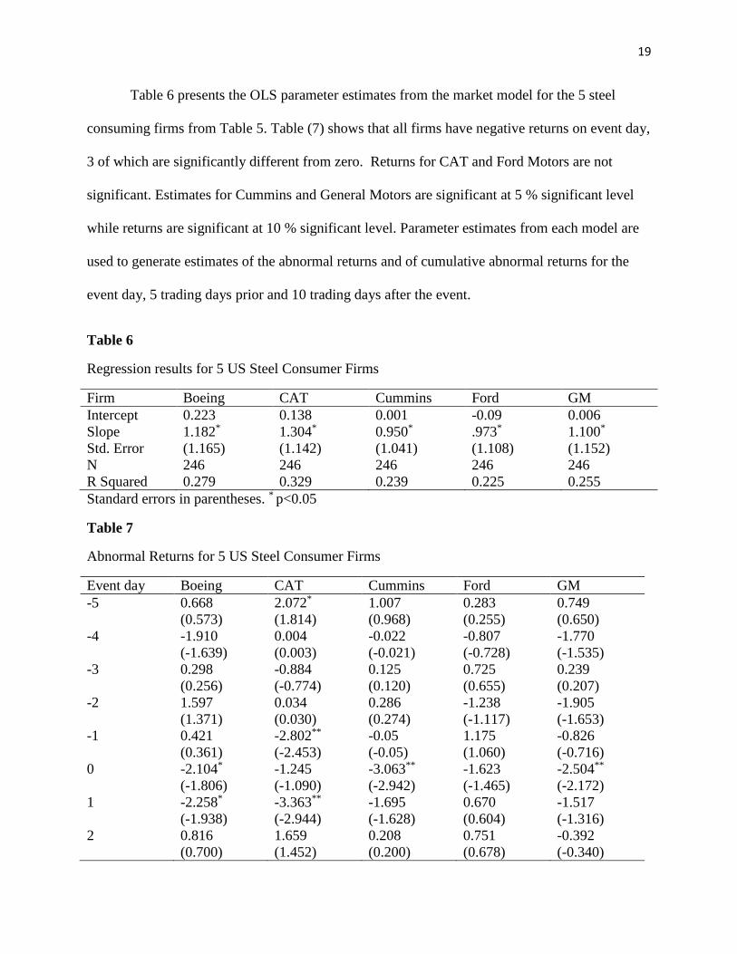
Table 5 provides the mean, min and max values for the 5 major US steel Consumers daily
returns and the Market Index. I also include a column for the number of estimation days for each
firm. The final column shows the standard deviations of the returns.
Table 5
Summary Statistics Percent Change in Daily Returns for 5 US Steel Consumer Firms
Firm N Mean (%) Min (%) Max (%) SD
Boeing 246 0.283 -5.740 9.879 1.372
CAT 246 0.204 7.860 -5.410 1.372
Cummins 246 0.049 -6.206 6.099 1.191
Ford 246 -0.043 -7.022 5.078 1.254
General Mot. 246 0.064 -3.868 5.867 1.335
S&P 500 246 0.050 -4.097 1.744 0.613
-60
-50
-40
-30
-20
-10
0
10
20
30
t -5 -4 -3 -2 -1 0 1 2 3 4 5 6 7 8 9 10
Nucor Steel Dyn US Steel CMC Carpenter Allgheny AK Steel
19
Table 6 presents the OLS parameter estimates from the market model for the 5 steel
consuming firms from Table 5. Table (7) shows that all firms have negative returns on event day,
3 of which are significantly different from zero. Returns for CAT and Ford Motors are not
significant. Estimates for Cummins and General Motors are significant at 5 % significant level
while returns are significant at 10 % significant level. Parameter estimates from each model are
used to generate estimates of the abnormal returns and of cumulative abnormal returns for the
event day, 5 trading days prior and 10 trading days after the event.
Table 6
Regression results for 5 US Steel Consumer Firms
Firm Boeing CAT Cummins Ford GM
Intercept 0.223 0.138 0.001 -0.09 0.006
Slope 1.182* 1.304* 0.950* .973* 1.100*
Std. Error (1.165) (1.142) (1.041) (1.108) (1.152)
N 246 246 246 246 246
R Squared 0.279 0.329 0.239 0.225 0.255
Standard errors in parentheses. * p<0.05
Table 7
Abnormal Returns for 5 US Steel Consumer Firms
Event day Boeing CAT Cummins Ford GM
-5 0.668
(0.573)
2.072*
(1.814)
1.007
(0.968)
0.283
(0.255)
0.749
(0.650)
-4 -1.910
(-1.639)
0.004
(0.003)
-0.022
(-0.021)
-0.807
(-0.728)
-1.770
(-1.535)
-3 0.298
(0.256)
-0.884
(-0.774)
0.125
(0.120)
0.725
(0.655)
0.239
(0.207)
-2 1.597
(1.371)
0.034
(0.030)
0.286
(0.274)
-1.238
(-1.117)
-1.905
(-1.653)
-1 0.421
(0.361)
-2.802**
(-2.453)
-0.05
(-0.05)
1.175
(1.060)
-0.826
(-0.716)
0 -2.104*
(-1.806)
-1.245
(-1.090)
-3.063**
(-2.942)
-1.623
(-1.465)
-2.504**
(-2.172)
1 -2.258*
(-1.938)
-3.363**
(-2.944)
-1.695
(-1.628)
0.670
(0.604)
-1.517
(-1.316)
2 0.816
(0.700)
1.659
(1.452)
0.208
(0.200)
0.751
(0.678)
-0.392
(-0.340)
20
3 -1.621
(-1.391)
1.257
(1.100)
-0.432
(-0.415)
0.310
(0.280)
0.206
(0.179)
4 -0.705
(-0.605)
-1.532
(-1.341)
-0.826
(-0.794)
0.142
(0.128)
-0.454
(-0.393)
5 -0.264
(-0.226)
0.651
(0.570)
-0.456
(-0.438)
-0.527
(-0.476)
0.787
(0.682)
6 -0.618
(-0.530)
0.627
(0.549)
0.337
(0.324)
-0.466
(-0.420)
-1.919
(-1.664)
7 -2.986**
(-2.563)
-2.342**
(-2.050)
-1.302
(-1.251)
0.964
(0.870)
0.107
(0.093)
8 -1.075
(-0.922)
0.167
(0.146)
0.784
(0.753)
0.437
(0.394)
1.169
(1.014)
9 -2.030
(-1.742)
-0.140
(-0.122)
0.081
(0.078)
2.878**
(2.598)
-0.218
(-0.189)
10 -0.216
(-0.185)
1.294
(1.132)
0.417
(0.401)
0.624
(0.564)
0.504
(0.437)
t-statistics in parentheses. * p<0.1, * *p<0.05, *** p<0.01
Table 8
Cumulative Abnormal Returns for 5 US Steel Consumer Firms
Event day Boeing CAT Cummins Ford GM
-5 0.668
(0.573)
2.072*
(1.814)
1.007
(0.968)
0.283
(0.255)
0.749
(0.650)
-4 -1.242
(-1.066)
2.077*
(1.818)
0.985
(0.946)
-0.523
(-0.472)
-1.021
(-0.885)
-3 -0.843
(-0.810)
1.192
(1.043)
1.111
(1.067)
0.201
(0.182)
0.781
(-0.678)
-2 0.653
(0.561)
1.226
(1.073)
1.397
(1.342)
-1.036
(-0.935)
-2.687**
(-2.331)
-1 1.075
(0.923)
-1.575
(-1.379)
1.339
(1.286)
0.138
(0.125)
-3.513**
(-3.047)
0 -1.029
(-0.883)
-2.821**
(-2.469)
-1.724
(-1.655)
-1.484
(-1.339)
-6.018**
(-5.220)
1 -3.288**
(-2.821)
-6.184**
(-5.413)
-3.419**
(-3.284)
-0.814
(-0.735)
-7.535**
(-6.536)
2 -2.471**
(-2.121)
-4.524**
(-3.960)
-3.211**
(-3.084)
-0.062
(-0.056)
-7.927**
(-6.876)
3 -4.093**
(-3.512)
-3.267**
(-2.860)
-3.643**
(-3.499)
0.247
(0.223)
-7.721**
(-6.697)
4 -4.798**
(-4.118)
-4.800**
(-4.201)
-4.470**
(-4.293)
0.390
(0.351)
-8.175**
(-7.091)
5 -5.063**
(-4.345)
-4.148**
(-3.631)
-4.927**
(-4.732)
-0.137
(-0.124)
-7.387**
(-6.408)
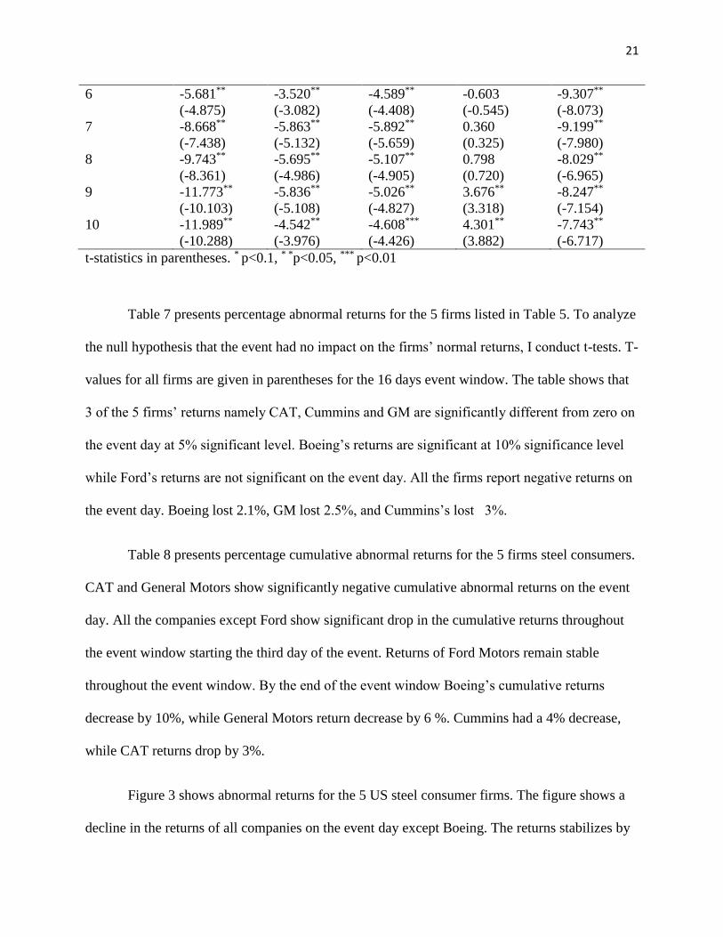
21
6 -5.681**
(-4.875)
-3.520**
(-3.082)
-4.589**
(-4.408)
-0.603
(-0.545)
-9.307**
(-8.073)
7 -8.668**
(-7.438)
-5.863**
(-5.132)
-5.892**
(-5.659)
0.360
(0.325)
-9.199**
(-7.980)
8 -9.743**
(-8.361)
-5.695**
(-4.986)
-5.107**
(-4.905)
0.798
(0.720)
-8.029**
(-6.965)
9 -11.773**
(-10.103)
-5.836**
(-5.108)
-5.026**
(-4.827)
3.676**
(3.318)
-8.247**
(-7.154)
10 -11.989**
(-10.288)
-4.542**
(-3.976)
-4.608***
(-4.426)
4.301**
(3.882)
-7.743**
(-6.717)
t-statistics in parentheses. * p<0.1, * *p<0.05, *** p<0.01
Table 7 presents percentage abnormal returns for the 5 firms listed in Table 5. To analyze
the null hypothesis that the event had no impact on the firms’ normal returns, I conduct t-tests. T-
values for all firms are given in parentheses for the 16 days event window. The table shows that
3 of the 5 firms’ returns namely CAT, Cummins and GM are significantly different from zero on
the event day at 5% significant level. Boeing’s returns are significant at 10% significance level
while Ford’s returns are not significant on the event day. All the firms report negative returns on
the event day. Boeing lost 2.1%, GM lost 2.5%, and Cummins’s lost 3%.
Table 8 presents percentage cumulative abnormal returns for the 5 firms steel consumers.
CAT and General Motors show significantly negative cumulative abnormal returns on the event
day. All the companies except Ford show significant drop in the cumulative returns throughout
the event window starting the third day of the event. Returns of Ford Motors remain stable
throughout the event window. By the end of the event window Boeing’s cumulative returns
decrease by 10%, while General Motors return decrease by 6 %. Cummins had a 4% decrease,
while CAT returns drop by 3%.
Figure 3 shows abnormal returns for the 5 US steel consumer firms. The figure shows a
decline in the returns of all companies on the event day except Boeing. The returns stabilizes by
22
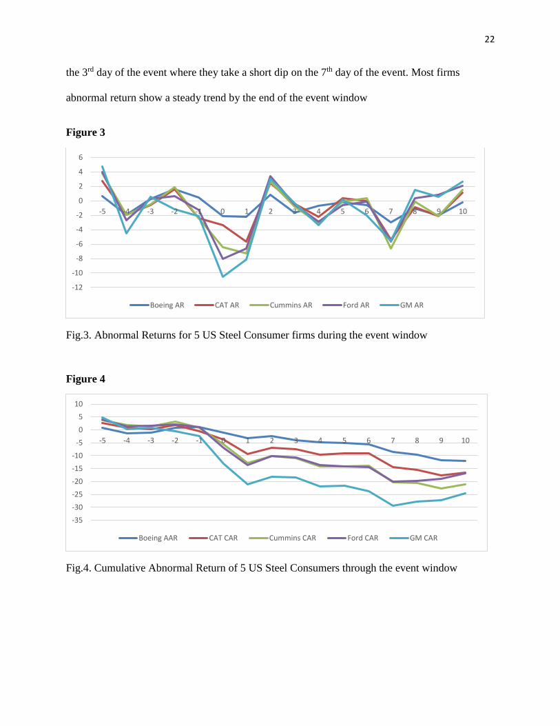
the 3rd day of the event where they take a short dip on the 7th day of the event. Most firms
abnormal return show a steady trend by the end of the event window
Figure 3
Fig.3. Abnormal Returns for 5 US Steel Consumer firms during the event window
Figure 4
Fig.4. Cumulative Abnormal Return of 5 US Steel Consumers through the event window
-12
-10
-8
-6
-4
-2
0
2
4
6
-5 -4 -3 -2 -1 0 1 2 3 4 5 6 7 8 9 10
Boeing AR CAT AR Cummins AR Ford AR GM AR
-35
-30
-25
-20
-15
-10
-5
0
5
10
-5 -4 -3 -2 -1 0 1 2 3 4 5 6 7 8 9 10
Boeing AAR CAT CAR Cummins CAR Ford CAR GM CAR
23
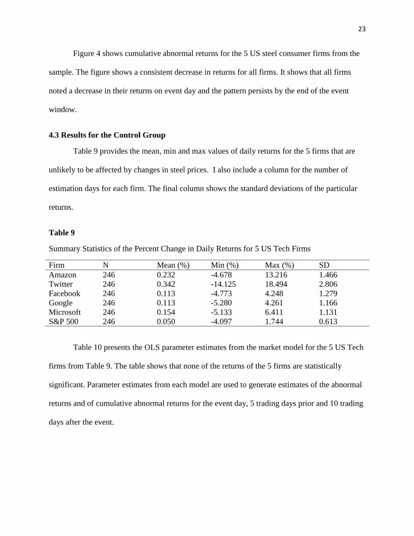
Figure 4 shows cumulative abnormal returns for the 5 US steel consumer firms from the
sample. The figure shows a consistent decrease in returns for all firms. It shows that all firms
noted a decrease in their returns on event day and the pattern persists by the end of the event
window.
4.3 Results for the Control Group
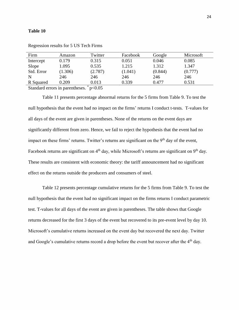
Table 9 provides the mean, min and max values of daily returns for the 5 firms that are
unlikely to be affected by changes in steel prices. I also include a column for the number of
estimation days for each firm. The final column shows the standard deviations of the particular
returns.
Table 9
Summary Statistics of the Percent Change in Daily Returns for 5 US Tech Firms
Firm N Mean (%) Min (%) Max (%) SD
Amazon 246 0.232 -4.678 13.216 1.466
Twitter 246 0.342 -14.125 18.494 2.806
Facebook 246 0.113 -4.773 4.248 1.279
Google 246 0.113 -5.280 4.261 1.166
Microsoft 246 0.154 -5.133 6.411 1.131
S&P 500 246 0.050 -4.097 1.744 0.613
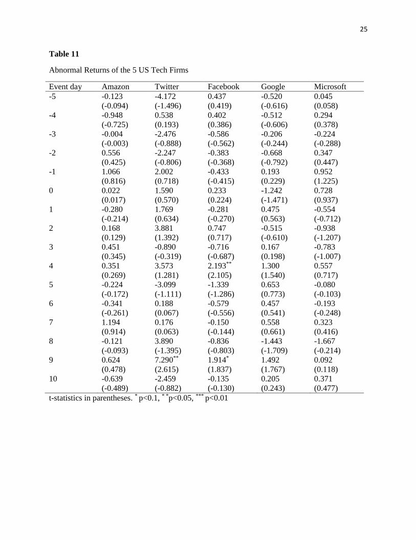
Table 10 presents the OLS parameter estimates from the market model for the 5 US Tech
firms from Table 9. The table shows that none of the returns of the 5 firms are statistically
significant. Parameter estimates from each model are used to generate estimates of the abnormal
returns and of cumulative abnormal returns for the event day, 5 trading days prior and 10 trading
days after the event.
24
Table 10
Regression results for 5 US Tech Firms
Firm Amazon Twitter Facebook Google Microsoft
Intercept 0.179 0.315 0.051 0.046 0.085
Slope 1.095 0.535 1.215 1.312 1.347
Std. Error (1.306) (2.787) (1.041) (0.844) (0.777)
N 246 246 246 246 246
R Squared 0.209 0.013 0.339 0.477 0.531
Standard errors in parentheses. * p<0.05
Table 11 presents percentage abnormal returns for the 5 firms from Table 9. To test the
null hypothesis that the event had no impact on the firms’ returns I conduct t-tests. T-values for
all days of the event are given in parentheses. None of the returns on the event days are
significantly different from zero. Hence, we fail to reject the hypothesis that the event had no
impact on these firms’ returns. Twitter’s returns are significant on the 9th day of the event,
Facebook returns are significant on 4th day, while Microsoft’s returns are significant on 9th day.
These results are consistent with economic theory: the tariff announcement had no significant
effect on the returns outside the producers and consumers of steel.
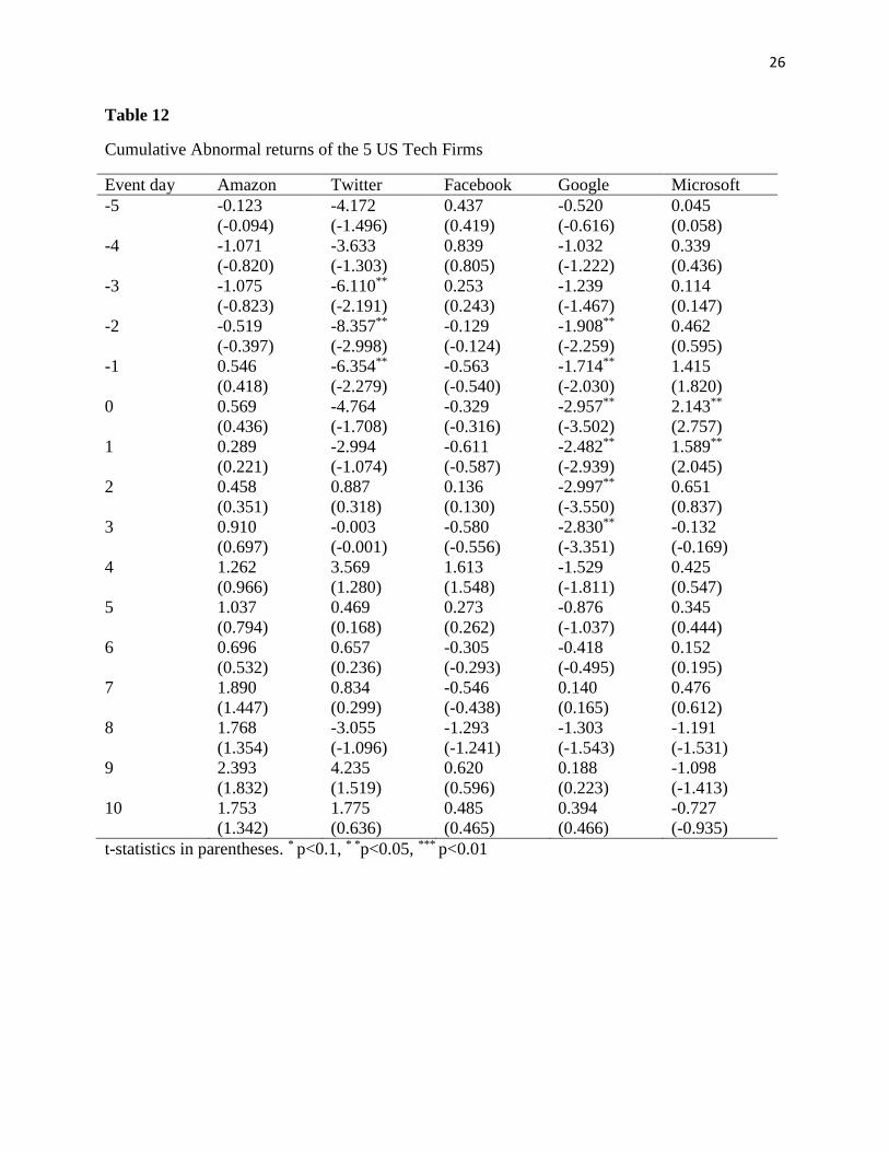
Table 12 presents percentage cumulative returns for the 5 firms from Table 9. To test the
null hypothesis that the event had no significant impact on the firms returns I conduct parametric
test. T-values for all days of the event are given in parentheses. The table shows that Google
returns decreased for the first 3 days of the event but recovered to its pre-event level by day 10.
Microsoft’s cumulative returns increased on the event day but recovered the next day. Twitter
and Google’s cumulative returns record a drop before the event but recover after the 4th day.
25
Table 11
Abnormal Returns of the 5 US Tech Firms
Event day Amazon Twitter Facebook Google Microsoft
-5 -0.123
(-0.094)
-4.172
(-1.496)
0.437
(0.419)
-0.520
(-0.616)
0.045
(0.058)
-4 -0.948
(-0.725)
0.538
(0.193)
0.402
(0.386)
-0.512
(-0.606)
0.294
(0.378)
-3 -0.004
(-0.003)
-2.476
(-0.888)
-0.586
(-0.562)
-0.206
(-0.244)
-0.224
(-0.288)
-2 0.556
(0.425)
-2.247
(-0.806)
-0.383
(-0.368)
-0.668
(-0.792)
0.347
(0.447)
-1 1.066
(0.816)
2.002
(0.718)
-0.433
(-0.415)
0.193
(0.229)
0.952
(1.225)
0 0.022
(0.017)
1.590
(0.570)
0.233
(0.224)
-1.242
(-1.471)
0.728
(0.937)
1 -0.280
(-0.214)
1.769
(0.634)
-0.281
(-0.270)
0.475
(0.563)
-0.554
(-0.712)
2 0.168
(0.129)
3.881
(1.392)
0.747
(0.717)
-0.515
(-0.610)
-0.938
(-1.207)
3 0.451
(0.345)
-0.890
(-0.319)
-0.716
(-0.687)
0.167
(0.198)
-0.783
(-1.007)
4 0.351
(0.269)
3.573
(1.281)
2.193**
(2.105)
1.300
(1.540)
0.557
(0.717)
5 -0.224
(-0.172)
-3.099
(-1.111)
-1.339
(-1.286)
0.653
(0.773)
-0.080
(-0.103)
6 -0.341
(-0.261)
0.188
(0.067)
-0.579
(-0.556)
0.457
(0.541)
-0.193
(-0.248)
7 1.194
(0.914)
0.176
(0.063)
-0.150
(-0.144)
0.558
(0.661)
0.323
(0.416)
8 -0.121
(-0.093)
3.890
(-1.395)
-0.836
(-0.803)
-1.443
(-1.709)
-1.667
(-0.214)
9 0.624
(0.478)
7.290**
(2.615)
1.914*
(1.837)
1.492
(1.767)
0.092
(0.118)
10 -0.639
(-0.489)
-2.459
(-0.882)
-0.135
(-0.130)
0.205
(0.243)
0.371
(0.477)
t-statistics in parentheses. * p<0.1, * *p<0.05, *** p<0.01
26
Table 12
Cumulative Abnormal returns of the 5 US Tech Firms
Event day Amazon Twitter Facebook Google Microsoft
-5 -0.123
(-0.094)
-4.172
(-1.496)
0.437
(0.419)
-0.520
(-0.616)
0.045
(0.058)
-4 -1.071
(-0.820)
-3.633
(-1.303)
0.839
(0.805)
-1.032
(-1.222)
0.339
(0.436)
-3 -1.075
(-0.823)
-6.110**
(-2.191)
0.253
(0.243)
-1.239
(-1.467)
0.114
(0.147)
-2 -0.519
(-0.397)
-8.357**
(-2.998)
-0.129
(-0.124)
-1.908**
(-2.259)
0.462
(0.595)
-1 0.546
(0.418)
-6.354**
(-2.279)
-0.563
(-0.540)
-1.714**
(-2.030)
1.415
(1.820)
0 0.569
(0.436)
-4.764
(-1.708)
-0.329
(-0.316)
-2.957**
(-3.502)
2.143**
(2.757)
1 0.289
(0.221)
-2.994
(-1.074)
-0.611
(-0.587)
-2.482**
(-2.939)
1.589**
(2.045)
2 0.458
(0.351)
0.887
(0.318)
0.136
(0.130)
-2.997**
(-3.550)
0.651
(0.837)
3 0.910
(0.697)
-0.003
(-0.001)
-0.580
(-0.556)
-2.830**
(-3.351)
-0.132
(-0.169)
4 1.262
(0.966)
3.569
(1.280)
1.613
(1.548)
-1.529
(-1.811)
0.425
(0.547)
5 1.037
(0.794)
0.469
(0.168)
0.273
(0.262)
-0.876
(-1.037)
0.345
(0.444)
6 0.696
(0.532)
0.657
(0.236)
-0.305
(-0.293)
-0.418
(-0.495)
0.152
(0.195)
7 1.890
(1.447)
0.834
(0.299)
-0.546
(-0.438)
0.140
(0.165)
0.476
(0.612)
8 1.768
(1.354)
-3.055
(-1.096)
-1.293
(-1.241)
-1.303
(-1.543)
-1.191
(-1.531)
9 2.393
(1.832)
4.235
(1.519)
0.620
(0.596)
0.188
(0.223)
-1.098
(-1.413)
10 1.753
(1.342)
1.775
(0.636)
0.485
(0.465)
0.394
(0.466)
-0.727
(-0.935)
t-statistics in parentheses. * p<0.1, * *p<0.05, *** p<0.01
27
Figure 5
Fig.5. Abnormal returns of the 5 US Tech firms throughout the event window
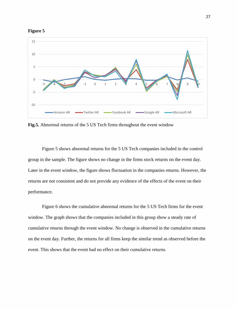
Figure 5 shows abnormal returns for the 5 US Tech companies included in the control
group in the sample. The figure shows no change in the firms stock returns on the event day.
Later in the event window, the figure shows fluctuation in the companies returns. However, the
returns are not consistent and do not provide any evidence of the effects of the event on their
performance.
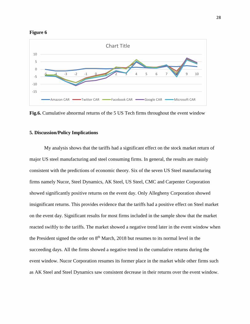
Figure 6 shows the cumulative abnormal returns for the 5 US Tech firms for the event
window. The graph shows that the companies included in this group show a steady rate of
cumulative returns through the event window. No change is observed in the cumulative returns
on the event day. Further, the returns for all firms keep the similar trend as observed before the
event. This shows that the event had no effect on their cumulative returns.
-10
-5
0
5
10
15
-5 -4 -3 -2 -1 0 1 2 3 4 5 6 7 8 9 10
Amazon AR Twitter AR Facebook AR Google AR Microsoft AR
28
Figure 6
Fig.6. Cumulative abnormal returns of the 5 US Tech firms throughout the event window
5. Discussion/Policy Implications
My analysis shows that the tariffs had a significant effect on the stock market return of
major US steel manufacturing and steel consuming firms. In general, the results are mainly
consistent with the predictions of economic theory. Six of the seven US Steel manufacturing
firms namely Nucor, Steel Dynamics, AK Steel, US Steel, CMC and Carpenter Corporation
showed significantly positive returns on the event day. Only Allegheny Corporation showed
insignificant returns. This provides evidence that the tariffs had a positive effect on Steel market
on the event day. Significant results for most firms included in the sample show that the market
reacted swiftly to the tariffs. The market showed a negative trend later in the event window when
the President signed the order on 8th March, 2018 but resumes to its normal level in the
succeeding days. All the firms showed a negative trend in the cumulative returns during the
event window. Nucor Corporation resumes its former place in the market while other firms such
as AK Steel and Steel Dynamics saw consistent decrease in their returns over the event window.
-15
-10
-5
0
5
10
-5 -4 -3 -2 -1 0 1 2 3 4 5 6 7 8 9 10
Chart Title
Amazon CAR Twitter CAR Facebook CAR Google CAR Microsoft CAR
29
This shows that the tariffs were not helpful for the steel firms as their market returns reduced
over the event window.
All of the US steel consuming firms except Boeing showed significantly negative returns
on the event day. The market resumes to the normal level in the next few days when they lose
market return again on March 08 when the President signed the tariff orders. Similarly, all firms
show a consistent decrease in cumulative returns over the event window. The result shows that
the tariffs harmed US steel consuming firms. When steel is a major raw material in a firm’s
production process ranging from automobile to construction industry, the result show that its
market value is harmed by the tariffs.
As for the control group, all the firms seem to be unaffected by the event. Their returns
are consistent with the market returns. This also indicates that the event was detrimental to the
steel firms and that the method we use to capture abnormal returns is robust enough to provide
significant results. Moreover, our results are consistent with the efficient market hypothesis in
this case as information spreads in one event interval as can be seen above in the analysis.
The results imply that contrary to the popular narrative portrayed by the Trump
administration that the tariffs are good for the economy and will save jobs in the indigenous
industry seems to be flawed and not supported by the evidence. A detailed investigation shows
that the effects might be otherwise portrayed by the political leadership. Tariffs increase the
prices of basic commodities in the market thus reducing the market returns of the firms listed on
stock market. This in turns results in lower revenue to the firms which will manifest in lower
dividends. The evidence shows that what we gain by giving protection to one sector at one place
is lost in other sectors, such that the overall loss exceeds the gain.
30
This is without accounting for the fact that tariffs once imposed lead to retaliatory
measures leading to trade wars that further harm welfare. Further, the ensuing trade wars while
increasing prices in the resultant markets lowers the surplus in all of the affected areas by tariffs.
Hence, this study also provides evidence in support of the economic principle that taxes (tariffs)
reduce overall surplus in the society leading to lower social welfare.
6. Conclusion
In this study, I used event study methodology to appraise the effects of the US steel
tariffs of March 2018 on producer value. Sixteen firms listed on the NYSE were included in the
study. These included 7 US steel manufacturing firms, 5 US steel consumer firms and a control
group that included 5 major US Tech firms. Most of the firms included in the sample showed
significant positive or negative abnormal returns on the day that tariff were announced.
Fluctuation in the returns indicates that investors reacted to the tariffs and that it affected the
market.
Future research may investigate the effects of other such tariffs that are imposed during
the Trump presidency in order to measure their effects on overall social welfare. Further, they
should investigate trade wars that tariffs cause. That may provide precise estimate of the possible
losses incurred as a result of the President’s general policy toward trade. Understanding the
social effects of tariffs will enable policy analysts to make informed decisions and better serve
the public.
31
7. References
Ball, R., & Brown, P. (1968). An empirical evaluation of Accounting income numbers. Journal of Accounting Research, 159-178.
Bhagat, S., & Romano, R. (2002a). Event Studies and the Law: Part 1: Technique and Corporate Litigation. American Law and Economics Review, 141-167.
Bhagat, S., & Romano, R. (2002b). Event Studies and the Law: Part 2: Empirical Studies of Corporate Law. American Law and Economics Review, 380-423.
Cornell, B., & Morgan, G. (1990). Using Finance Theory to Measure Damages in Fruad on the Market Cases. UCLA Law Review, 883-924.
Corrado, C. (2011). Event Studies: A methodological Review. Journal of Accounting and Finance, 207-234.
Fama, E., Fisher, L., Jensen, M., & Roll, R. (1969). The Adjustment of Stock Prices to New Information. International Economic Review, 1-21.
Gokhale, J., Brooks, R., & Tremblay, V. (2014). The effect on Stockholer Wealth of product recalls and government action: The case of Toyota's accelerator pedal recall. The Quarterly Review of Economics and Finance, 1-8.
Jaher, J., & Pugh, W. (1991). State Takeover Legislation: The case of Delaware. Journal of Law, Economics and Regulation, 410-428.
Jarrel, G. (1984). Change at the Exchange: The Causes and Effects of Deregulation. The Journal of Law and Economics, 273-312.
Jarrell, G., & Peltzman, S. (1985). The Impact of Product Recalls on the wealth of sellers. Journal of Political Economy, 512-536.
Jarrell, G. (1984). Change at the Exchange: The Causes and Effects of Deregulation. The Journal of Law and Economics, 273-312.
MacKinlay, C. (1997). Event Studies in Economics and Finance. Journal of Economic Literature, 13-39.
Romano, R. (1990). Corporate Governance in the Aftermath of of the Insurance Crisis. Emory Law Review, 1155-89.
Serra, A. (2004). Event Study Tests: A brief Survey. Gestao.Org, 248-255.
Thomsen, M., & McKenzie, A. (2001). Market Incentives for safe foods: An examination of shareholers losses from meat and poultry recalls. American Journal of Agriculture Economics, 526-538.