AN ABSTRACT OF THE ESSAY OF

Matthew Perreault for the degree of Master of Public Policy presented on June 8, 2020.

Title: Revitalization of Gentrification?: An Examination of Urban Renewal Areas and

Housing Instability in Oregon.

Abstract approved:

______________________________________________________

Patrick Emerson

Housing affordability is a salient topic among policymakers and the general public

today, especially in Oregon. As housing costs continue to rise, there are concerns that

urban planning policies such as urban renewal via tax-increment financing (TIF) are

exacerbating the problem and pushing more households into a state of housing

instability. This study examines whether there is a systematic difference in the

number of cost-burdened households in urban renewal areas (URAs) in Oregon

compared with areas outside of URAs. It also attempts to discern whether the

duration of a URA’s existence has any effect on the levels of cost-burdened

households in that area. Results show that census tracts that contain urban renewal

areas are associated with approximately 5% more cost-burdened households than

census tracts without urban renewal areas, with levels as high as 20% higher for rent-

burdened households in these areas. However, there is no evidence that these high

levels of cost-burdened households change across the duration of a URA’s existence.

While further research is needed to determine causal effects, the persistence of

elevated levels of cost burdens in URAs is cause for concern for policymakers.

©Copyright by Matthew Perreault

June 8, 2020

All Rights Reserved

Revitalization or Gentrification?: An Examination of Urban Renewal Areas and

Housing Instability in Oregon

by

Matthew Perreault

AN ESSAY

submitted to

Oregon State University

in partial fulfillment of

the requirements for the

degree of

Master of Public Policy

Presented June 8, 2020

Commencement June 2020

Master of Public Policy essay of Matthew Perreault presented on June 8, 2020

APPROVED:

Patrick Emerson; Major Professor, representing Economics

Mark Edwards; representing Sociology

Scott Akins; representing Sociology

I understand that my thesis will become part of the permanent collection of Oregon

State University libraries. My signature below authorizes release of my thesis to any

reader upon request.

Matthew Perreault, Author

ACKNOWLEDGEMENTS

I would like to express my sincere appreciation for those who helped me

accomplish this project. Thank you to Patrick Emerson, my committee chair, who

advised me throughout this process from the beginning.

Thanks to Brent Steel, Mark Edwards, Scott Akins, Alison Johnston, and the

rest of the faculty at the School of Public Policy, whose teaching was invaluable.

I would also like to extend thanks to Kate Porsche, whose professional

expertise is a credit to the City of Corvallis and the School of Public Policy.

Thanks to Alethia Miller for inspiring me to start this journey.

Thank you to my mom for her undying love and encouragement. It is because

of her that I consider myself to be a lifelong learner.

Lastly, thank you to my wife, my partner in life, whose sacrifices, love, and

support made this all possible.

TABLE OF CONTENTS

Page

I. Introduction ................................................................................................................................. 1

II. Background and Literature Review............................................................................................ 3

Background ................................................................................................................................... 3

Urban Renewal in Oregon ............................................................................................................... 3

Tax Increment Financing ................................................................................................................ 4

Literature Review ........................................................................................................................... 6

Tax Increment Financing ................................................................................................................ 6

Gentrification and Displacement ...................................................................................................... 7

Housing Insecurity ...................................................................................................................... 10

Theoretical Framework ................................................................................................................. 12

III. Data and Methods ................................................................................................................... 16

Data Sources and Coding .............................................................................................................. 16

Descriptive Statistics .................................................................................................................... 19

Model Specification and Hypotheses ............................................................................................... 21

Model Robustness ....................................................................................................................... 28

IV. Findings .................................................................................................................................. 32

Primary Findings .......................................................................................................................... 32

Secondary Findings ...................................................................................................................... 36

Tertiary Findings .......................................................................................................................... 42

V. Discussion ................................................................................................................................ 45

VI. Limitations .............................................................................................................................. 47

VII. Conclusion ............................................................................................................................. 49

References ..................................................................................................................................... 51

Appendices .................................................................................................................................... 54

Appendix A: Urban Renewal Areas in Oregon ............................................................................... 55

Appendix B: Percentage Point Regression Results .......................................................................... 60

Appendix C: Negative Binomial Regression Results ....................................................................... 61

Appendix D: Auxiliary Regression Results .................................................................................... 62

LIST OF FIGURES

Figure Page

Figure 1…………………………………………………….…………………………5

Figure 2……………………………..………………………………………………..14

Figure 3…………………………..…………………………………………………..15

Figure 4……………………………..………………………………………………..32

Figure 5…………………..…………………………………………………………..36

Figure 6………………………………………………………………………………39

Figure 7………..……………………………………………………………………..39

Figure 8………………….…………………………………………………………...42

Figure 9……………………………………………..…………………….………….42

Figure 10……………………………...……………………………………………...42

LIST OF TABLES

Table Page

Table 1………………………………………………………………………………20

Table 2……………………………………………………………………..………..21

Table 3……………………………………………………………………………....34

Table 4……………………………………………...……………………………….38

Table 5……………………………………………...……………………………….41

Table 6……………………………………………...……………………………….44

LIST OF APPENDIX TABLES

Table Page

Table A1 …………………………………………………………………55

Table A2……………………………………………………………….....60

Table A3……………………………………………………………….....61

Table A4……………………………………………………………….....62

DEDICATION

For my wife Hannah, who can make me laugh like no one else.

1

I. Introduction

Decades after the era of white flight, cities are once again emerging as the country’s

cultural and economic centers. As cities continue to grow, rising prices and scarce land has led to

housing becoming increasingly unaffordable for many residents. Consequently, the “global

housing affordability crisis” has become an increasingly salient concern for citizens and

policymakers alike (Wetzstein, 2017). While states and cities implement new laws to strengthen

legal protections for vulnerable households in response to this crisis, other longstanding policies

for urban planning and economic development have come under scrutiny as counterproductive

drivers of gentrification and displacement. One such policy is urban renewal by means of tax-

increment financing (TIF), a tool used by municipalities to redevelop areas of cities that have

historically experienced disinvestment, poverty, and blight. Proponents of TIF tout its

effectiveness as a tool for raising tax revenue without increasing tax rates on property owners,

which allows for a public intervention in an economically depressed area that results in greatly

improved outcomes for the community. Critics cite its power as a force for gentrification and

displacement, historically clearing out entire neighborhoods and redeveloping them in order to

attract wealthier residents and businesses. As more cities in Oregon and elsewhere continue to

express interest in adopting TIF for economic development, it is worth investigating what impact

it may have on housing instability and whether it contributes to gentrification and displacement

of vulnerable residents.

Rising housing costs in the last decade have given rise to concerns of the increasing

unaffordability of housing and associated social consequences, such as inequality, poverty, and

2

homelessness. This study seeks to examine whether urban renewal areas (URAs) in Oregon that

are financed by TIF are associated with increased levels of housing instability. Because the

purpose of urban renewal is to target “blighted” areas for redevelopment and increase the

assessed value of property in the area, I hypothesize that urban renewal areas are associated with

disproportionately higher levels of cost-burdened households, which are defined as households

that allocate more than 30% of their income to housing costs. However, this alone will not

determine what impact urban renewal has on housing instability. In addition, I examine a

hypothesized association between cost-burdened households and the duration of a URA’s

existence in order to determine the impact of urban renewal over time. The paper is organized as

follows. Section II lays out the historical and institutional background of urban renewal policy in

Oregon, the theoretical framework for this study’s methodology, and a review of the literature on

the topics of gentrification, displacement, and housing instability. Section III describes the

methodology and data used in this study, while section IV presents my findings. Section V

discusses the results through the lens of theory. Section VI discusses limitations of the study’s

methodology and makes recommendations for future research. Section VII discusses larger

policy implications of my findings and concludes.

3

II. Background and Literature Review

Background

Urban Renewal in Oregon

Urban renewal has a complex history in the world of public policy. Often, the term is

associated with the large-scale federally funded redevelopment and infrastructure projects of the

1950s and 1960s. These projects arose from the federal Housing Act of 1949, an initiative to

reverse decades of decline and blight in the country’s urban centers in the wake of the Great

Depression and the Second World War (Hoffman, 2000). In spite of the legislation’s progressive

policy goals of alleviating poverty and replacing substandard housing with new public housing

units, the urban renewal projects of this era have been widely documented as slum-clearing

events that displaced tens of thousands of residents in low-income neighborhoods across the

United States, widening racial and income disparities while entrenching local business elites as

powerful drivers of economic policy and city planning (Gotham, 2000, 2001).

In Portland, Oregon, voters authorized the creation of the Portland Development

Commission (PDC, now called Prosper Portland), a quasi-independent public agency with a

streamlined organizational structure that enabled rapid and often clandestine deals with real

estate developers (Gibson, 2004). Under the leadership of businessman Ira Keller, the PDC

initiated the South Auditorium urban renewal project in 1957, which cleared out a neighborhood

in that city’s downtown for new public construction, displacing the area’s mainly Jewish and

Italian residents and businesses (Campos, 1979; Gibson, 2004; Wollner et al., 2001). At the same

time, urban renewal efforts and freeway construction in the north and northeast sections of the

city displaced thousands of residents in the Albina neighborhood, which was home to more than

4

50% of the city’s African American population (Wollner et al., 2001). By the late 1960s, public

opposition to further displacement halted the city’s plans for freeway expansion in Southeast

Portland, forcing the city to reconsider its approach to urban renewal and adopt a more

consensus-driven approach that accommodated public input (Campos, 1979). However, people

of color continued to be disproportionately affected by urban renewal policy; it is estimated that

more than 10,000 Black residents were displaced from the Albina area as a result of the Interstate

Corridor Urban Renewal Area between 1990 and 2016 (Hughes, 2019).

Tax Increment Financing

Today, contemporary urban renewal policy in Oregon is conducted via tax-increment

financing (TIF), a mechanism designed to capture and redirect property tax revenues in order to

fund public investments without raising nominal tax rates. State law empowers a municipality to

create an independent urban renewal agency, which is charged with carrying out redevelopment

efforts in a “blighted” area, meaning an area with depressed property values, poor planning,

inadequate services or infrastructure, substandard or abandoned structures, or conditions that

generate more expenses for public services than they bring in tax revenue (ORS 475.10). The

urban renewal agency addresses its mission by capping the total assessed value of all properties

within the boundaries of its purview, allowing a fixed amount of tax revenue to flow to tax

authorities in the boundaries while accruing any excess tax revenue to fund its redevelopment

activities, as shown in Figure 1 (Brimmer & Fitzgerald, 2019, pp. 18-19). Thus, the agency is

incentivized to engage in activities that maximize return on investment and grow the tax base by

increasing property values in the targeted area, with the aims of eliminating blight and

revitalizing the local economy. These activities include condemning derelict or dilapidated

properties, funding infrastructure projects such as streetlights and water mains, partnering with

5

property developers to build new housing units, environmental cleanup, offering incentives to

attract employers to the area, and sponsoring grants to encourage new businesses to open.

Eventually, if the efforts at economic revitalization are successful, the agency is dissolved and

the frozen tax revenue cap is removed, yielding significantly more revenue to the taxing

authorities than was foregone during the period of urban renewal (Tax Increment Finance Best

Practices Reference Guide, 2007).

Annual Taxes

Generated ($)

Years

Frozen Tax Base (to

taxing authorities)

Incremental Tax Revenue

(to UR agency)

URA Begins

New Tax Base

(to taxing

authorities)

URA Ends

Adapted from Tax Increment Finance

Best Practices Reference Guide

(2007, p. 2)

Figure 1

6

Literature Review

Tax Increment Financing

An urban renewal agency’s activities are expected to spur economic revitalization that

would not occur “but for” a public intervention in the private market (Dye & Merriman, 2000, p.

310). Therefore, it can be understood to be correcting a market failure in the form of under-

provisioned public goods (Brueckner, 2001). However, this raises concerns of opportunity costs,

unintended consequences, and perverse incentives. For example, this type of market-oriented

redevelopment rarely results in direct displacement of residents in the area via eminent domain;

rather, rising property values and changing neighborhood characteristics may indirectly result in

the displacement of residents through gentrification. This is a concern among practitioners of

urban renewal in the state of Oregon (Best Practices for Tax Increment Financing Agencies in

Oregon, 2019, pp. 12-17), but there is little in the way of empirical research that directly ties TIF

to higher rates of displacement or housing insecurity.

Brueckner (2001) demonstrates the qualities of TIF as a mechanism for provisioning

public goods while sidestepping local opposition to property tax increases, concluding that it is

effective in doing so only if the public good is moderately or severely under-provisioned (i.e., the

area is sufficiently blighted). However, the TIF intervention is not necessarily efficient and may

result in over-provisioning of the public good beyond the socially optimal level. For example, if

we understand neighborhood quality to be a public good, an urban renewal intervention via TIF

may succeed in transforming a blighted neighborhood into one that is more desirable, resulting in

a neighborhood that attracts wealthier individuals from beyond the immediate area who bid up

properties and replace the existing residents, a process known as gentrification. Luque (2020)

7

theorizes that TIF could efficiently enable cities to increase the supply of affordable housing

despite an inflationary effect on construction costs.

A pair of empirical studies on TIF note its effects on property value appreciation (Dye &

Merriman, 2000; Man & Rosentraub, 1998). Man and Rosentraub (1998) employ a two-stage

first-differences model that estimates the effect that TIF districts have on property value growth,

finding that cities with TIF districts see rates of owner-occupied property growth that are on

average 11% higher than those that do not. By contrast, Dye and Merriman (2000) find a much

more conservative 2% increase and note the endogeneity of self-selection of TIF as a biasing

factor in this effect, as anticipation of property value growth in a TIF district may be driving

itself rather than any direct intervention. After controlling for this endogeneity, they conclude

that a TIF district largely redirects economic activity from elsewhere while having a negative net

effect on economic development. Therefore, areas targeted for urban renewal are revitalized at

the expense of other areas in a trade-off. Weber, et al. (2007) found that housing price

appreciation varies significantly depending on the type and purpose of a given TIF district—

industrial and commercial developments had a negative effect, while mixed-use developments in

a downtown or central area have a positive effect. This spillover effect decreases with distance

from the TIF district, implying that owners of property nearest to new TIF-funded developments

such as mixed-use condominium/retail buildings are most likely to see property value

appreciation. The authors conclude that policy remedies to address the increased cost burden

may be necessary to counteract downstream effects of price increases in housing.

Gentrification and Displacement

The term “gentrification” was coined in 1964 by Ruth Glass, who lamented the

“invasion” of working-class areas of London by the middle classes, which she attributed to the

8

forces of postwar urban revitalization and laissez-faire deregulation (Glass, 2013). Thus,

gentrification is generally understood to be a process by which a “working-class or vacant area”

of a city is transformed into “middle-class residential and/or commercial use” (Slater, 2009, p.

294). This is typically believed to be a change in the demographic makeup of a central urban

neighborhood by which residents of low socioeconomic status (SES), who often belong to racial

or ethnic minority groups, are replaced by relatively affluent, predominantly white newcomers.

These newcomers bid up housing prices, eventually displacing the original residents who can no

longer afford to live there. This is connected to a phenomenon known as the “back-to-the-city

movement,” as urban areas formerly abandoned by middle-class households during the era of

“white flight” are now experiencing population influxes that fundamentally alter their

demographic and cultural makeup (Hyra, 2015). It remains the subject of much debate in

academic and popular literature.

The urban studies literature on the consequences of gentrification is extensive, and there

remains a persistent divide in findings and conclusions between the positivist and critical areas of

the field. Influential studies by Vigdor (2002) and Freeman and Braconi (2004) published

empirical results suggesting that gentrification appeared to lessen the likelihood of low-SES

households being displaced and to improve general quality of life. Freeman (2005) found a small

displacement effect, but its magnitude is minimal when compared to non-gentrifying areas with

similar characteristics where housing instability may already be common. This contributed to a

popular narrative that gentrification does not significantly harm residents by displacing them, but

rather yields beneficial outcomes for those residents in the form of improved neighborhood

quality and higher incomes, reducing the likelihood of displacement (Hampson, 2005). However,

these authors acknowledge the difficulty of detecting such effects using econometric methods,

9

particularly the task of accurately measuring displacement. While demographic change in a

given area is easily observable from surveys and Census data, understanding displacement is

more difficult, particularly determining to what degree such displacement may be involuntary

rather than an expression of preferences. Nevertheless, these authors caution against drawing

conclusions that gentrification is harmless and emphasize the importance of policy responses to

address broad issues of inequality. These studies left an impact in the field that continue to

resonate today: A recent study by Martin and Beck (2018) replicates the methods used by

Freeman (2005) and finds that homeowners are not significantly impacted by gentrification in

neighborhoods in the way that renters might be. They speculate that this non-effect among

homeowners may be driving much of the non-significant findings in previous studies on

gentrification, suggesting that further research do more to differentiate the heterogenous

pressures of gentrification on homeowners and renters.

A body of more critical research on gentrification provides substantial evidence of

detrimental effects on poor residents, particularly in Newman and Wyly (2006). These authors

replicate the methods and findings in Freeman and Braconi (2004), finding a significant but

small statistical effect, then follow up with in-depth interviews with the residents of those

neighborhoods, revealing a much richer set of findings. Interview participants noted the “mixed

blessing” of improving neighborhood conditions but fear that they will be displaced by rising

rents or evictions (Newman & Wyly, 2006, p. 45). Many reported increasing reliance on public

housing assistance to stay in their homes, while others noted a trade-off between housing quality

and affordability (p. 49). In seeking to reconcile their findings, the authors speculate that

displacees disappear from data systems once they become homeless or move outside of the city;

they also note that the unique and complex system of housing protections in New York City may

10

be a mitigating factor, suggesting that gentrification-induced stresses may be worse in other

places with fewer protections. A follow-up study by Wyly, et al. (2010) further explores these

possibilities by conducting a comprehensive logistic prediction model that attempts to determine

the factors most likely to contribute to displacement. They find that, perhaps unsurprisingly, poor

renters are most at risk of displacement, particularly those with rent-to-income ratios much

higher than average. Elderly renters are particularly at risk, while non-significant coefficients on

race, gender, and family size suggested an intersection of entangled variables related to inner-

city poverty. Most importantly, the authors emphasize the disappearance of rent-regulated and

affordable housing, an important bulwark against displacement in gentrifying areas, as a product

of long-running campaigns of deregulation and debt-fueled real estate speculation prior to the

Great Recession. Findings in these studies have inspired writers such as Slater (2009) to

advocate for the “decommodification” of housing as a financial asset and to restore social justice

as a priority in understanding the seriousness of gentrification and its effects on city residents.

Housing Insecurity

It is clear that while gentrification may contribute to increased affordability pressure on

low-SES residents in urban neighborhoods, its impact may be concentrated on the most housing-

insecure households in the area. There remains considerable debate among researchers as to the

definition of housing insecurity. A recent article in Cityscape, the U.S. Department of Housing

and Urban Development’s (HUD) academic research journal, lamented the absence of a standard

operational definition of the concept, resulting in a myriad of terms such as “housing insecurity,”

“housing instability,” “housing affordability,” et cetera, each of which are measured and defined

differently (Cox et al., 2019). The head author of that piece also recently attempted to

operationalize a multidimensional categorical index for housing insecurity in an attempt to

11

determine to what extent they share characteristics, finding that poverty, singlehood, Black and

Hispanic ethnicity, foreign-born noncitizen status, and less education were significant drivers of

higher housing insecurity, while older adults experienced lower housing insecurity (Cox et al.,

2017).

Despite the fragmented state of this body of research, the cost-to-income ratio approach

remains common, particularly among government bodies. Known as the “cost burden” metric or

the ratio approach, this is defined as a household spending more than 30% of its income on

housing costs. This approach has its basis in federal housing policy and is the threshold for many

public housing assistance programs (Schwartz & Wilson, 2008). Some government bodies, such

as HUD, further define “severe cost burden” as spending more than 50% of household income on

housing expenses, a critical component characteristic for that agency’s “worst case housing

needs” (Elsasser Watson et al., 2017). However, as discussed previously, a higher proportion of

household income devoted to housing may simply be an expression of individual preferences.

Thalmann (1999) estimates that two out of three burdened households could afford less

expensive housing and argues that they are not truly in need of public assistance. However,

Thalmann does not consider whether phenomena such as gentrification might be driving housing

cost inflation for these households, or that households seeking more affordable housing

elsewhere might be a result of displacement in a changing and increasingly expensive

neighborhood.

Housing policy scholars have put forward alternatives to address the deficiencies of the

ratio approach. The most well-known of these alternatives is Stone’s “shelter poverty,” which

suggests a residual income approach that compares a household’s share of income after

subtracting housing expenses to a fixed bundle of expenses such as the consumer price index (M.

12

E. Stone, 2004, 2010, 2010). Kutty (2005) offers a similar concept, finding that nearly 4.3% of

non-poverty households appeared to suffer from a form of housing-induced poverty. This effect

appeared more in the Northeast and West regions of the country; renters, particularly elderly

renters, were particularly at risk.

These findings echo similar indicators of the types of households most vulnerable to the

forces of gentrification: Renters, particularly elderly renters, in relatively expensive regions of

the country, who are not receiving any public assistance or lack the benefits of housing

protections, are particularly vulnerable to housing cost burdens and displacement. What remains

unclear is whether urban renewal efforts, such as the tax-increment financing districts used in

Oregon elsewhere, are responsible for worsening the conditions of these households through

deliberate inflation in the property market.

Theoretical Framework

With these concepts now established, it is necessary to frame how I chose to analyze their

interconnected nature. This framework is a blend of the critical urban theory found in Slater

(2009), Newman and Wyly (2006), and others with neoclassical economic theory and

econometric methodologies from the likes of Vigdor (2002). Assume the supply of housing in a

neighborhood to be inelastic in the short run (shown in Figure 2). An exogenous increase in

demand for housing in the neighborhood, perhaps driven by improved neighborhood quality as a

result of urban renewal, shifts the demand curve rightward, resulting in an increase of the

equilibrium price of rental housing. This is expressed by renters seeing steep increases in

contract rents. A renter household, facing a budget constraint, must choose between remaining in

their home, thus reducing consumption of other goods at a sub-optimal level of utility, or

relocating to a less expensive home in a different neighborhood or city, as shown in Figure 3

13

(Vigdor, 2002, p. 141). If enough households choose to relocate rather than pay higher rents, the

demographics of the neighborhood will change considerably, a reflection of gentrification.

Alternatively, poor households may not face a choice at all: If there are no affordable housing

units in the area, or if moving is prohibitively expensive, relocating may be out of the question,

so the household must cut back spending on other goods. If these non-housing “other goods” are

essentials such as food and clothing are no longer affordable, the household can be described as

experiencing “shelter poverty” (M. E. Stone, 2004) or “housing-induced poverty” (Kutty, 2005),

a key indicator of housing insecurity.

Vigdor (2002) noted that the general equilibrium effects of gentrification may not result

in a net loss of utility for poor households. If urban renewal produces new job opportunities for

local residents to increase their income, or if new investment in the area leads to improvements

in neighborhood quality or safety, residents may decide that higher housing costs are worth

paying for increased quality of life. It is risky to assume, however, that the original residents in a

gentrifying neighborhood may be able to weather higher housing cost burdens long enough to

enjoy the benefits of neighborhood improvement. Therefore, a municipality seeking to pursue an

urban renewal project may face a perverse incentive: boosting property values may attract

higher-SES households to the area, bring more tax revenue to fund investments without raising

nominal tax rates, and generate knock-on effects in the local economy, but at the risk of

displacing residents of that area or pushing them into a state of poverty.

14

Figure 2

Housing Stock

Price of Housing ($)

D0

D1

A

B

S

15

Figure 3

Other Goods

BL0 BL1

U0

U2

U1

A

B

C

Adapted from Vigdor (2002, p. 141)

Housing

16

III. Data and Methods

Data Sources and Coding

In order to examine whether there is an effect from urban renewal policies via tax-

increment financing districts on housing insecurity, thus contributing to gentrification and

displacement, I analyzed a series of cross-sectional regression models using data from the 2018

American Community Survey (ACS) and the Oregon Department of Revenue’s property tax

statistics (Brimmer & Fitzgerald, 2019). Data gathered from the 2018 ACS included counts and

percentages of households for a variety of statistics at the census tract level in the state of Oregon

(N=834), including population, median income, racial and ethnic demographics, economic and

employment statistics, and housing conditions and costs. Data from the Oregon Department of

Revenue included a cross-section of every active urban renewal area in Oregon in the 2018-2019

fiscal year (N=122). Importantly, I wanted to assess the impact of urban renewal across the entire

state, encompassing multiple urban areas as well as non-urban areas, rather than a single city.

Because my objective was to determine whether urban renewal areas exert any isolated

influence on housing affordability or insecurity, I sought to operationalize a quantitative variable

from the available data that would serve as a proxy for these concepts. While the 30% cost-to-

income metric seemed an obvious choice, there is plenty of literature highlighting its drawbacks

and suggesting alternative metrics, such as the residual income approach favored by Kutty

(2005) and Stone (2010). However, given the well-established tradition of the 30% cost-burden

rule in public policy, despite its shortcomings, I decided to proceed with operationalizing

housing affordability using this standard, particularly because of the ease with which I could

obtain it from the American Community Survey dataset. In the future, housing policy researchers

ought to continue to explore alternative metrics and operationalizations that capture the

17

complications of housing affordability and insecurity, such as the residual income approach or

the multidimensional approach used by Cox et al. (2017).

Thus, the primary dependent variable in my analysis is cost burden, a composite variable

that captures the total count of households in a given census tract in Oregon that pays more than

30% of its income toward housing costs. The 2018 ACS provides counts and percentages of

households with “gross rent as a percentage of income” (GRAPI) and “selected monthly owner

costs as a percentage of income” (SMOCAPI) divided into ordinal categories demarcated by

five-percentage-point increments. My primary cost burden variable combines the count values

from both the GRAPI and SMOCAPI categories in the 30.0-34.9% range and the 35% and over

range in order to obtain a total count in each census tract of the number of households that pays

30% or more of income toward housing costs. My secondary dependent variables for cost-

burdened renters and cost-burdened homeowners are respectively defined as the counts of strictly

GRAPI and SMOCAPI in the 30-34.9% and 35% and over categories. Because the ACS data did

not provide more detailed data on housing cost burdens beyond the 30% and over category, I was

not able to operationalize the concept of “severe cost burden” as defined by HUD; this remains a

topic for future research.

I coded each census tract with a binary URA variable that took the value of 1 if a census

tract contained any part of an urban renewal area and 0 if it did not. In order to do this, I cross-

referenced these urban renewal areas by visually matching their locations with the census tracts

they overlaid using the Census Bureau’s online geographic tool with each jurisdiction’s most

recently amended urban renewal plan. This required me to obtain each of the 122 urban renewal

plan documents in order to review each plan’s map of URA boundaries, taking care to ensure

that each map included any amendments from the original urban renewal plan that may have

18

amounted since the plan was first adopted. My criteria for coding census tracts consisted of

careful comparison of the map area in each urban renewal plan with the Census Bureau’s census

tracts map, assessing whether any part of a URA fell within the boundaries of each census tract.

In a few instances, the URA plan maps were not detailed enough to accurately compare to the

satellite photos in the Census Bureau’s geographic tool, and thus necessitated a judgment call. In

some cases, only a single building, street, or tax lot fell within a census tract that otherwise did

not contain a URA; I coded these tracts as URA = 1 in order to consistently account for the

influence that urban renewal areas have on the resident population’s economic and housing

security. In only one case, a URA overlaid a census tract with no resident population. If a census

tract was overlaid by more than one urban renewal district, it remained coded as 1.

I also coded each census tract with a continuous URA Years variable that took the value

of the difference between the year 2018 and the year that the urban renewal area in that tract was

adopted by its jurisdiction (such as the city council or county commission). Thus, this variable

represents the duration in years that a URA existed in each census tract through the year 2018. If

a census tract contained more than one urban renewal area, the duration of the URA that was

adopted first was used as the basis for this calculation. It is important to note that jurisdictions

have the power to amend urban renewal plans to add or remove land, and in some cases, it is

possible that an urban renewal area expanded into a census tract in the intervening years since its

original adoption, therefore a census tract coded as 1 for URA may not have actually contained

an urban renewal area for the entire duration of that URA’s existence. Due to the difficulty and

time necessary to thoroughly parse the fluidity of the URA amendment process by calculating

the precise duration a census tract may have existed in each census tract, I assumed each tract’s

URA duration value as static, while acknowledging that it is possible that each tract may not

19

have literally contained a URA for its entire duration. This is a limitation that may bias

regression results toward the null hypothesis, but it is also possible that any possible bias might

be mitigated by spillover effects.

Descriptive Statistics

Of the 834 census tracts in Oregon for which I collected data, 298 tracts contained some

or all of an urban renewal area and thus were coded URA = 1, while 536 tracts did not and were

coded URA = 0. The continuous URA Years variable, which preserves the 0 values from the

binary URA variable but replaces the 1 values with the number of years that a URA existed in

each census tract, has a mean of 5.78, standard deviation of 9.66, and a maximum of 50. On

average, census tracts that contain URAs exhibit higher levels of cost-burdened households than

those without URAs, as shown in Table 1. The mean value for cost-burdened households in a

non-URA census tract is approximately 685, while that value for a census tract in a URA is

approximately 820, which is nearly 18% higher. For renters, the ratio is approximately 308 to

437, a difference of nearly 35%, while for homeowners it is 377 to 383, a 1.61% difference. The

large differences for overall households and renters are in spite of the fact that the difference in

mean population between to two groups is just 5.54% higher for tracts in URAs. Also notable is

that the median income in census tracts with URAs is approximately 16% lower than that in non-

URA tracts on average, while median property values are 10.36% lower in tracts with URAs.

Tracts with URAs also have on average 3.63% more households that reported living in the same

home a year prior than tracts without URAs. Lastly, tracts with URAs also contain significantly

higher populations of non-White people, higher rates of poverty, and more households that

receive public assistance benefits.

20

VARIABLE

No URA (N=536)

Mean (Std. dev.)

URA (N=298)

Mean (Std. dev.) Difference (%)

Cost-burdened Households (all) 684.77 (342.34) 819.98 (388.97) 17.97

Cost-burdened Renters 307.55 (269.97) 436.64 (314.39) 34.69

Cost-burdened Homeowners 377.22 (208.043) 383.34 (203.25) 1.61

Population over age 16 3893.57 (1691.56) 4115.50 (1624.98) 5.54

Median Income

$66,399.27

(24932.33)

$56,600.50

(19404.85) -15.93

Median Property Value

$278,734.30

(106860.5)

$251,272.60

(99435.72) -10.36

Housing Stability 3934.48 (1784.82) 4079.94 (1782.94) 3.63

Unemployment (%) 6.03 (3.15) 6.50 (3.53) 7.51

# on Public Assistance 63.86 (62.12) 84.30 (68.08) 27.59

Poverty (%) 8.50 (6.15) 11.30 (8.06) 28.28

Single Parents 139.54 (101.84) 171.49 (119.52) 20.54

College Education 1161.85 (876.80) 1057.26 (785.31) -9.43

Veterans 344.86 (194.78) 347.98 (204.97) 0.90

Disabled 663.49 (357.96) 768.28 (377.28) 14.64

Non-English Speakers 646.49 (697.90) 825.61 (797.27) 24.34

Black pop. 74.65 (135.52) 126.77 (215.39) 51.75

Native American pop. 57.54 (167.91) 54.09 (61.01) -6.17

Hispanic pop. 559.01 (647.78) 752.78 (779.098) 29.54

New Housing 84.78 (104.44) 92.06 (115.24) 8.24

Share of renters (%) 33.57 (18.55) 38.88 (18.47) 14.67

Table 2 displays pairwise correlation coefficients for selected variables in the dataset.

The first column shows the correlations between the cost burden dependent variable and

hypothesized explanatory variables. The binary URA indicator variable shares a positive

correlation with cost burden (r=0.1775), further reinforcing the hypothesis that more cost-

burdened households exist in census tracts that contain urban renewal areas. The coefficient is

slightly higher for renters (r=0.2112), while it is much lower and statistically insignificant for

homeowners (r=0.0142). Importantly, cost burden is also strongly correlated with population

(r=0.579), suggesting the possibility that a higher level of cost burdened households may simply

be a function of greater overall population in a census tract. The cost burden

Table 1

21

variable is negatively correlated with median income (r=-0.2971), which is also in line with

expectations. The URA variable is also negatively correlated with median income (r=-0.1998)

and median property value (r=-0.1256), which is also expected given that areas with URAs are

expected to exhibit indicators of “blight”.

Model Specification and Hypotheses

Because these variables are largely correlated with each other, attempting to isolate their

effect on a particular dependent variable using statistical inference could potentially result in

non-significant or nonsensical results due to multicollinearity, endogeneity or misdirected causal

order. Therefore, care must be taken when specifying regression models that accurately represent

the hypothetical relationship between these variables. I experimented with a variety of model

specifications given the data available, which included counts variables and percentage-point

variables. It should be emphasized that these two types of variables are different conceptually

despite appearing side-by-side in the ACS dataset, as a count variable yields a raw number of

VARIABLE Cost

Burden

(all)

Cost

Burden

(renters)

Cost Burden

(homeowners)

URA

(binary)

URA

Duration

(years)

Population

over age

16

Median

Income

Median

Property

Value

Housing

Stability

Cost Burden

(all)

1

Cost Burden

(renters)

0.8257*** 1

Cost Burden

(homeowners)

0.5978*** 0.0414 1

URA (binary) 0.1775*** 0.2112*** 0.0142 1

URA

Duration

(years)

0.1714*** 0.2244*** -0.0154 0.8028*** 1

Population

over age 16

0.579*** 0.5118*** 0.2982*** 0.0637* 0.0136 1

Median

Income

-0.2971*** -0.2889*** 0.0270 -0.1998*** -0.2089*** 0.0587* 1

Median Property

Value

0.0248 -0.0373 0.0986** -0.1256*** -0.0575* 0.0417 0.3402*** 1

Housing

Stability

0.4617*** 0.3406*** 0.3337*** 0.0391 -0.0429 0.9465*** 0.1513*** 0.0296 1

Table 2

*** p<0.01, ** p<0.05, * p<0.1

22

households in a given census tract while a percentage-point variable yields a share of the total

number of households in that census tract; therefore, count variables offer much more potential

for variation while percentage-point variables are bounded between 0 and 100. While it may

seem beneficial to model for percentage-point variables, particularly as a dependent variable, as

a means of bypassing the driving force of population increases that may underlie higher-value

counts, I ultimately found that models specified with only percentage-point variables did not

produce meaningful results when compared with alternative specifications.1 In addition, using

the raw counts variable for cost burden allowed me to construct a composite variable that is the

sum of the households in each census tract whose GRAPI or SMOCAPI is greater than 30%.

This would not be possible with the percentage-point variables and would thus require me to

estimate values for renters and homeowners in separate regression models. Of course, any

estimates based on counts data must account for underlying population growth, which I handle

by including each census tract’s population as a control variable in my models.

Therefore, I proceeded to specify an ordinary least squares (OLS) regression model using

the counts variables provided in the ACS, with a few exceptions. The final regression model is as

follows:

ln(𝑐𝑜𝑠𝑡 𝑏𝑢𝑟𝑑𝑒𝑛𝑖) = 𝛼 + 𝛽𝑈𝑅𝐴𝑖 + 𝛾ln(𝚾𝑖) + 𝛿𝚭𝑖 + 휀𝑖

On the left-hand side of the equation, the dependent variable is cost burden, the count of

households in census tract i whose housing expenses are greater than 30% of their income. I

decided to transform this variable using the natural logarithm to aid in interpretation of the

estimated regression coefficient magnitudes, as log-transformations allow marginal effects to be

approximated to percentage changes in the dependent variable. Furthermore, logarithmic

1 Results from these alternative specifications are printed in the Appendix.

23

transformations of both dependent and independent variables allow for interpretation of

approximate elasticities between the variables (%y/%x). The primary regression model

specifies the composite cost burden variable for all cost-burdened households, while additional

regression models specify cost-burdened renters and cost-burdened homeowners separately. All

models are specified with the natural-logarithm transformation of these dependent variables.

The right-hand side of the equation specifies the independent explanatory variables in the

model. The independent variable of interest is the binary indicator variable URA, which takes the

value of 1 if census tract i contains any part of an urban renewal area and 0 otherwise. The

coefficient estimates the average conditional linear effect of the URA variable on the dependent

variable, holding all other variables constant. In other words, if census tract i contains an urban

renewal district, the number of cost-burdened households would change by approximately %,

all else being equal. I hypothesize that this coefficient will have a positive sign, as census tracts

that contain URAs are expected to exhibit higher levels of cost-burdened households than census

tracts that are outside of URAs.

The remaining terms on the right-hand side of the equation are additional explanatory

variables added to the model as controls. is a vector of large-value economic and demographic

variables that are expected to exhibit miniscule or undetectable effects if their coefficients were

interpreted at the margin—variables such as population, median income, and median property

value. Taking the natural logarithm of these variables is a common tactic that allows for

interpretation of percentage changes rather than single-unit or marginal changes. Because the

dependent variable is also transformed by the natural logarithm, the coefficient is interpreted as

an elasticity. is a vector of additional control variables that include additional demographic,

economic, and social factors—these include the counts of households that receive public

24

assistance, single-parent households with children, households with college-educated members,

veterans, disabled individuals, households that speak a language other than English, households

that are entirely Black, Native American, or Hispanic, the number of households living in the

same home as the year before (hereafter referred to as “housing stability”), and the number of

houses constructed since 2005 (hereafter referred to as “new construction”). This vector also

includes some percentage-point variables, such as the unemployment rate, the poverty rate, and

the proportion of renters in census tract i. Because these variables are untransformed and are

either raw counts or percentage points, the coefficient is interpreted as a marginal linear effect

on the dependent variable, or the percentage by which cost burden changes with a 1-unit increase

in the explanatory variable. Lastly, is a stochastic error term that accounts for random

fluctuations and unaccounted-for variation in census tract i.

In this model specification, the coefficient on the binary URA indicator variable is the

primary term of interest. The gentrification hypothesis states that urban renewal areas are a

driving factor in intensifying housing insecurity among vulnerable populations in underserved

and blighted neighborhoods. Conversely, the economic development hypothesis states that any

housing stress would predate the establishment of an urban renewal district and that such

conditions would be alleviated over time as the urban renewal district accomplishes its goals. I

therefore construct my primary hypotheses as follows:

𝐻𝑜: 𝛽 ≤ 0

𝐻𝐴: 𝛽 > 0

I decided to construct my hypotheses so that the economic development hypothesis is the null—

the default assumption is that urban renewal as public policy is accomplishing its goals as a

driver of property value growth and economic development with minimal unintended

25

consequences in the form of increased housing stress; hence, successful urban renewal policy in

these areas produces minimal or even less housing insecurity than areas without such

interventions, reflected by a coefficient that is 0 or negative. The alternative is the

gentrification hypothesis—that higher property values and housing prices driven by urban

renewal areas are responsible for placing additional pressure in the form of higher housing costs

on vulnerable populations in neighborhoods that are targeted for urban renewal, reflected in a

significant and positive coefficient.

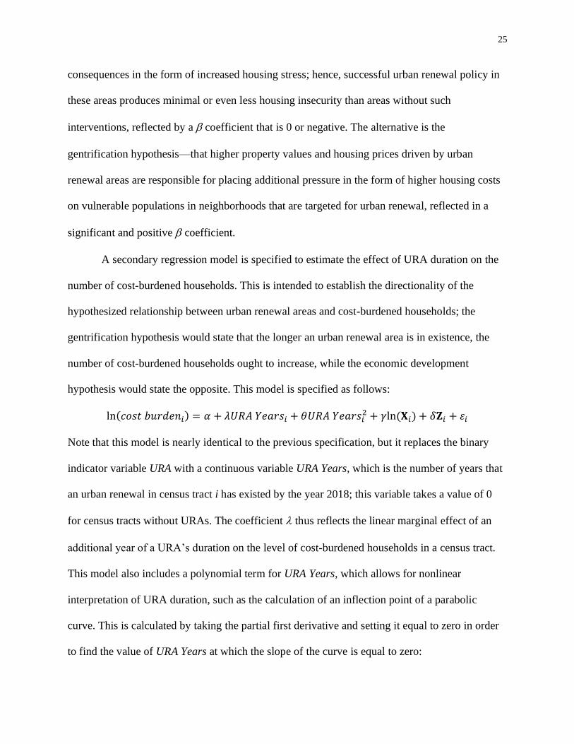
A secondary regression model is specified to estimate the effect of URA duration on the

number of cost-burdened households. This is intended to establish the directionality of the

hypothesized relationship between urban renewal areas and cost-burdened households; the

gentrification hypothesis would state that the longer an urban renewal area is in existence, the

number of cost-burdened households ought to increase, while the economic development

hypothesis would state the opposite. This model is specified as follows:

ln(𝑐𝑜𝑠𝑡 𝑏𝑢𝑟𝑑𝑒𝑛𝑖) = 𝛼 + 𝜆𝑈𝑅𝐴 𝑌𝑒𝑎𝑟𝑠𝑖 + 𝜃𝑈𝑅𝐴 𝑌𝑒𝑎𝑟𝑠𝑖2 + 𝛾ln(𝚾𝑖) + 𝛿𝚭𝑖 + 휀𝑖

Note that this model is nearly identical to the previous specification, but it replaces the binary

indicator variable URA with a continuous variable URA Years, which is the number of years that

an urban renewal in census tract i has existed by the year 2018; this variable takes a value of 0

for census tracts without URAs. The coefficient thus reflects the linear marginal effect of an

additional year of a URA’s duration on the level of cost-burdened households in a census tract.

This model also includes a polynomial term for URA Years, which allows for nonlinear

interpretation of URA duration, such as the calculation of an inflection point of a parabolic

curve. This is calculated by taking the partial first derivative and setting it equal to zero in order

to find the value of URA Years at which the slope of the curve is equal to zero:

26

𝜕ln (𝑐𝑜𝑠𝑡 𝑏𝑢𝑟𝑑𝑒𝑛)

𝜕𝑈𝑅𝐴 𝑌𝑒𝑎𝑟𝑠= 𝜆 + 2𝜃𝑈𝑅𝐴 𝑌𝑒𝑎𝑟𝑠 = 0

Rearranging terms, the formula for an inflection point becomes:

𝑈𝑅𝐴 𝑌𝑒𝑎𝑟𝑠∗ =−𝜆

2𝜃

If the sign on the coefficient is positive, it suggests that the parabolic curve is hump-shaped; in

other words, as URA duration increases in years, the level of cost-burdened households initially

increases until reaching the inflection point, after which the level starts to fall. Conversely, if the

sign on is negative, the curve is U-shaped, and the opposite effect occurs. Thus, the inflection

point is the critical feature of interpretation in this model as it allows for a more complex and

nonlinear relationship between URA duration and cost-burdened households. The vectors and

are identical to the previous model specification. It should be noted that due to the

overrepresentation of 0 values in this model specification as a result of the 536 observations in

the sample that are not census tracts with URAs, OLS results from this regression estimation

could be biased. To address this potential bias, I also specify the model by restricting the sample

to the observations that are coded as URA=1 (N=298) to attempt to improve accuracy at the

expense of the precision afforded by the full sample. Results from both specifications are

reported in the following section.

In order to further establish the direction of causality between housing insecurity and

urban renewal, this secondary model specification replaces the binary URA indicator variable

with a continuous URA Years variable which captures the duration that an urban renewal district

has existed in census tract i along with corresponding linear coefficient . It also adds a

polynomial URA Years term with nonlinear coefficient . I test both linear and nonlinear

27

specifications of this model separately to consider hypothesized relationships between URA

duration and cost burdens. The linear hypotheses are constructed as follows:

𝐻𝑜: 𝜆 ≤ 0

𝐻𝐴: 𝜆 > 0

Similar to the previous hypotheses, the null hypothesis establishes the economic development

argument and states that, as URA duration increases in years, the level of cost burden is not

impacted or reduced; hence, is either 0 or negative. The alternative hypothesis establishes the

gentrification argument that cost burden levels will rise as the duration of a URA’s existence

increases in years; hence, is positive.

The nonlinear hypotheses are constructed in order to establish a more complex

relationship between URA duration and cost burdens. In theorizing a quadratic relationship

between the URA duration and cost burden variables, we allow for the latter to both rise and fall

as URA duration increases in years. Therefore, the coefficient of interest is that on the quadratic

term in the equation, . The hypotheses for this coefficient are stated as follows:

𝐻𝑜: 𝜃 < 0

𝐻𝐴: 𝜃 > 0

A negative sign on implies a hump-shaped curve when plotting the bivariate relationship

between cost burden and URA duration. As in prior models, the null hypothesis continues to

follow the economic development argument, in this case allowing cost burden to first rise and

then fall as urban renewal areas accomplish their goals of improving blight and poverty in the

neighborhood. The alternative hypothesis follows the gentrification argument, which concedes

that while short-term gains may be made by urban renewal in the form of lower cost burdens,

eventually the forces of gentrification take hold and increase the cost burdens and therefore

28

housing insecurity of the residents affected by the URA, reflected by the U-shaped curve formed

by a positive sign on . If = 0 or is not statistically significant, this invalidates the hypothesized

quadratic relationship between URA duration and cost burdens, rather implying the linear

relationship expressed by the coefficient. A nonzero coefficient allows calculation of an

inflection point, or the value of URA Years at which cost burden levels either stop rising and start

to fall, or vice versa.

Model Robustness

Estimating relationships between variables via Ordinary Least Squares (OLS) regression

relies on a set of assumptions collectively known as the Gauss-Markov Theorem. In short, OLS

regression models are assumed to be correctly specified linear models whose variables are

parsimonious (i.e., no irrelevant variables), exogenous (i.e., no omitted relevant variables), free

of multicollinearity (i.e., variables are uncorrelated with each other), and whose errors are

homoscedastic (i.e., the error term has a constant variance). As a method for statistical inference,

OLS is the best linear unbiased estimator (BLUE) only if these assumptions are fulfilled; if they

are violated, regression estimates calculated with OLS are biased either in their coefficients or

standard errors and OLS is no longer BLUE. In order to ensure the accuracy of my results, I

subjected my regression models to a series of robustness checks designed to test the fulfillment

of these assumptions. I also compared OLS results against alternative estimators and

specifications to confirm their consistency.

Violation of the perfect multicollinearity assumption precluded me from including the

binary URA variable and the continuous URA Years variable in the same models, as a 0 value for

URA perfectly correlates to a 0 value for URA Years; thus, the models needed to be estimated

separately. Imperfect multicollinearity among other explanatory variables was detected by noting

29

the significant nonzero pairwise correlation coefficients displayed in Table 2 and calculating the

variance inflation factors (VIF) for these variables. A particularly strong case of imperfect

multicollinearity was discovered between the population and stability variables; however, in

final results, both variables retained strong significance and did not largely impact the

significance of other variables in the model, so this issue was left unchanged. As a result of this

decision, estimated standard errors are no longer ideally efficient but the estimated coefficients

are still unbiased.

The homoscedasticity assumption was also likely violated according to the results of a

White test, suggesting that estimated standard errors in the base OLS model were biased

downward, thereby overstating statistical significance. I re-estimated the models with HC3

robust standard errors to counteract this bias. All results in the next section are reported with

these conservatively robust standard errors. Additionally, the normality of error distribution,

necessary for hypothesis testing, was confirmed by plotting a histogram of the predicted

residuals against a normal curve.

There are fewer concrete solutions to address the assumptions of exogeneity and absence

of relevant omitted variables. There is also often a trade-off between adding more potentially

relevant variables (at the expense of parsimony) and introducing multicollinearity between

variables that share correlation. A Ramsey RESET test, often used to test for the appropriateness

of higher-order polynomial terms in a regression model, returned a result that suggested such

variables were necessary. Apart from the quadratic URA Years term, however, no other variable

in the dataset appeared to be a logical candidate for such a specification. As the selection of

explanatory variables in my models was guided by theory and prior literature, I elected to ignore

this result while acknowledging the possible existence of additional omitted variables that could

30

explain variation in household cost burdens. The same is true for the exogeneity assumption:

While it is possible that cost burden levels are endogenous to the creation of URAs, I attempted

to isolate the causal order by estimating the effect of URA duration in a second model after

establishing the systematic significance of URAs in the first model. While there are more

sophisticated methods for doing this, such as the two-stage instrumental variable models

employed Man and Rosentraub (1998) and Dye and Merriman (2000), I believe my results are

valid and easy to interpret while conceding that further research utilizing more advanced

techniques would be worth pursuing.

Lastly, I compared the OLS estimations against those from an alternative method for

estimating counts variables using Negative Binomial Regression. This method allows for

nonlinear specifications between variables and produce estimates in terms of factor changes of

predicted counts, and it relaxes some assumptions that are necessary for producing valid

estimates with OLS. Because my primary OLS models employ a counts-based dependent

variable, it was relatively simple to compare results. The estimated factor changes in these

models were nearly identical to those in the OLS models, further substantiating the accuracy of

the estimates in those OLS models.2 I therefore decided to proceed with reporting the results in

the OLS models as my primary model specification.

Because it is unrealistic to expect statistical estimation of real-world social phenomena

using pseudo-experimental methodology to perfectly fulfill these assumptions as cleanly as a

laboratory experiment, it is essential to test for and address violations of the classical OLS

assumptions. I believe that by doing so, I have presented evidence to support the validity of my

findings. However, there are opportunities for future researchers to further disentangle the

2 Results from the Negative Binomial Regression model are printed in the Appendix.

31

concerns of endogeneity and casual directionality, perhaps by employing time-series or

instrumental variables estimation methods. Nevertheless, I selected robust model specifications

that best withstood tests of the core assumptions while retaining explanatory power (via

relatively high R2 and F values) and parsimony (via relatively low values for Aikake and

Bayesian information criteria). The results for these regression models are presented in the

following section.

32

IV. Findings

Primary Findings

Results from the

primary regression models are

shown in Table 3. The

coefficient estimate on the URA

indicator variable is positive

and significant at a 95%

confidence level, which is

consistent with the

gentrification hypothesis that

levels of cost burdens are higher in census tracts with urban renewal areas than those without.

My core finding is that census tracts that contain urban renewal areas (URAs) are

estimated to have levels of cost-burdened households that are 5% higher than census tracts that

are outside of URAs. This accounts for increases in population, income, and a host of

demographic and economic control variables. In other words, approximately 5% more of the

households in a census tract that contains a URA experience a housing-cost burden compared to

a demographically identical tract that is outside of a URA, all else being equal. It is also

important to note the strong positive elasticity between population and cost-burdened

households, as would be expected. In this model, a 1% increase in population translates to a

0.9% increase in cost-burdened households, a nearly 1-to-1 elastic relationship. This is crucial to

maintain the validity of this model in order to demonstrate that a higher level of cost-burdened

households is not simply a function of larger population. However, it is notable that the elasticity

Figure 4

33

is 1.64 for cost-burdened renters, suggesting that a 1% increase in the population yields a 1.64%

increase in the number of cost-burdened renters, which is likely a result of greater population

density in more urbanized areas of the state. In addition, there is a negative elasticity of 0.52

between cost-burdened households and a census tract’s median income, meaning that a 1%

increase in the median income translates to a 0.52% decrease in the number of cost-burdened

households. This result is also unsurprising, as wealthier census tracts would be less likely to

exhibit high levels of cost burdened households. Most of the signs on the remaining coefficients

are also in line with expectations and generally reflect what we would expect as indicators of

financial insecurity and social inequality. However, contrary to expectations, there appears to be

a negative correlation between unemployment and cost burdened renters.

34

Table 3

Cost Burden (log)

VARIABLES Total Renters Homeowners

URA in Census Tract 0.0572** (0.0232) 0.191*** (0.0339) 0.0234 (0.0336)

Population (log) 0.898*** (0.0965) 1.636*** (0.159) 0.411*** (0.123)

Median Income (log) -0.525*** (0.0627) -1.197*** (0.102) 0.0645 (0.0902)

Median Property Value in

$ (log)

0.0779** (0.0340) 0.0464 (0.0521) -0.00245 (0.0497)

Unemployment (%) -0.00587 (0.00414) -0.0203*** (0.00721) 0.00445 (0.00582)

# on Public Assistance 0.000700*** (0.000260) 0.00139*** (0.000487) 0.000241 (0.000372)

Poverty (%) 0.00624** (0.00291) 0.00570 (0.00532) 0.00758** (0.00357)

Single Parents 0.000785*** (0.000150) 0.00234*** (0.000265) -0.000165 (0.000226)

College Education 0.000183*** (2.48e-05) 0.000411*** (4.27e-05) -5.20e-06 (3.33e-05)

Veterans -0.000362*** (0.000102) -0.000550*** (0.000185) -0.000140 (0.000152)

Disabled 5.42e-05 (6.51e-05) 3.51e-05 (0.000121) 6.55e-05 (9.65e-05)

Housing Stability -0.000132*** (2.37e-05) -0.000298*** (3.82e-05) -5.83e-06 (3.23e-05)

Non-English Speakers -1.02e-06 (3.14e-05) -1.65e-05 (5.14e-05) 9.10e-06 (4.06e-05)

Black pop. 0.000125* (7.32e-05) 5.19e-05 (0.000111) 0.000243** (0.000104)

Native American pop. -0.000329*** (0.000111) -0.000494** (0.000248) -0.000261 (0.000202)

Hispanic pop. 3.92e-05 (3.19e-05) 6.27e-05 (5.60e-05) 5.38e-06 (3.77e-05)

New Housing 0.00111*** (0.000104) -0.000187 (0.000229) 0.00169*** (0.000156)

Share of renters (%) -0.00590*** (0.000867) 0.00361*** (0.00116) -0.0164*** (0.00115)

Constant 4.208*** (1.201) 4.986*** (1.757) 2.095 (1.540)

Observations 813 813 813

R-squared 0.661 0.720 0.468

HC3 robust standard errors in parentheses

*** p<0.01, ** p<0.05, * p<0.1

35

The differences between URAs and non-URAs are even more stark when the model is

changed to measure cost burdens of renters and homeowners separately, as seen in Figure 4.

These separate models suggest that the relationship between urban renewal and housing cost

burdens are not distributed evenly between homeowners and renters. When analyzed separately

by housing tenure, tracts with URAs yield a 20% higher level of cost-burdened renters compared

to those outside of URAs; meanwhile, there is no measurable effect for cost-burdened

homeowners. This is a significant finding, and one that is supported by the literature (Martin &

Beck, 2018). This suggests that renters are heavily impacted in areas that contain urban renewal

areas while homeowners are not. According to the gentrification hypothesis, urban renewal areas

will yield higher property values, which disproportionately benefit individuals who own property

at the expense of those who pay rent to those owners. While homeowners may benefit from

increased property values that result from urban renewal efforts, renters must cope with higher

rents by allocating a larger share of their income toward housing costs. Conversely, the theory

behind the economic development hypothesis would reverse the causal order to suggest that the

heavier presence of housing insecurity in URAs is indicative of the blight that urban renewal is

attempting to resolve. Therefore, the number of cost-burdened households ought to decrease over

time as development efforts in these blighted areas improves conditions for vulnerable

populations through interventions such as public safety and affordable housing.

At first glance, these results seem to favor the gentrification hypothesis—that urban

renewal areas are responsible for placing additional housing stress on the vulnerable populations

that often live in economically depressed areas, rather than alleviating such stress through

economic development. However, it does not definitively prove a causal relationship; indeed, the

causal order might very well be reversed, suggesting that census tracts with higher levels of cost-

36

burdened households are more likely to be declared urban renewal areas. At the very least, this

finding confirms that the areas with urban renewal in place are systematically different from

areas without it in ways that are not explained by changes in population, income, or other

demographic characteristics. We must therefore investigate further by examining whether the

duration of a URA’s existence has any effect on housing cost burden. In addition, I examine the

effect of URAs on income, property values, and housing stability.

Secondary Findings

In order to test this secondary

hypothesis, I conducted additional

regression analysis using models

that replace the URA dummy

variable with a continuous

variable that records the duration

in years that the oldest URA in

that census tract has existed. The

URA duration variable is defined

as the year that the jurisdiction

adopted its urban renewal plan subtracted from the year 2018, the survey year from this cross-

section of the American Community Survey. This variable preserves the 0 values from the binary

URA dummy variable. The table also shows models that include a quadratic URA years variable

to test whether there is a non-linear relationship between the duration of a URA and housing cost

burdens.

Figure 5

37

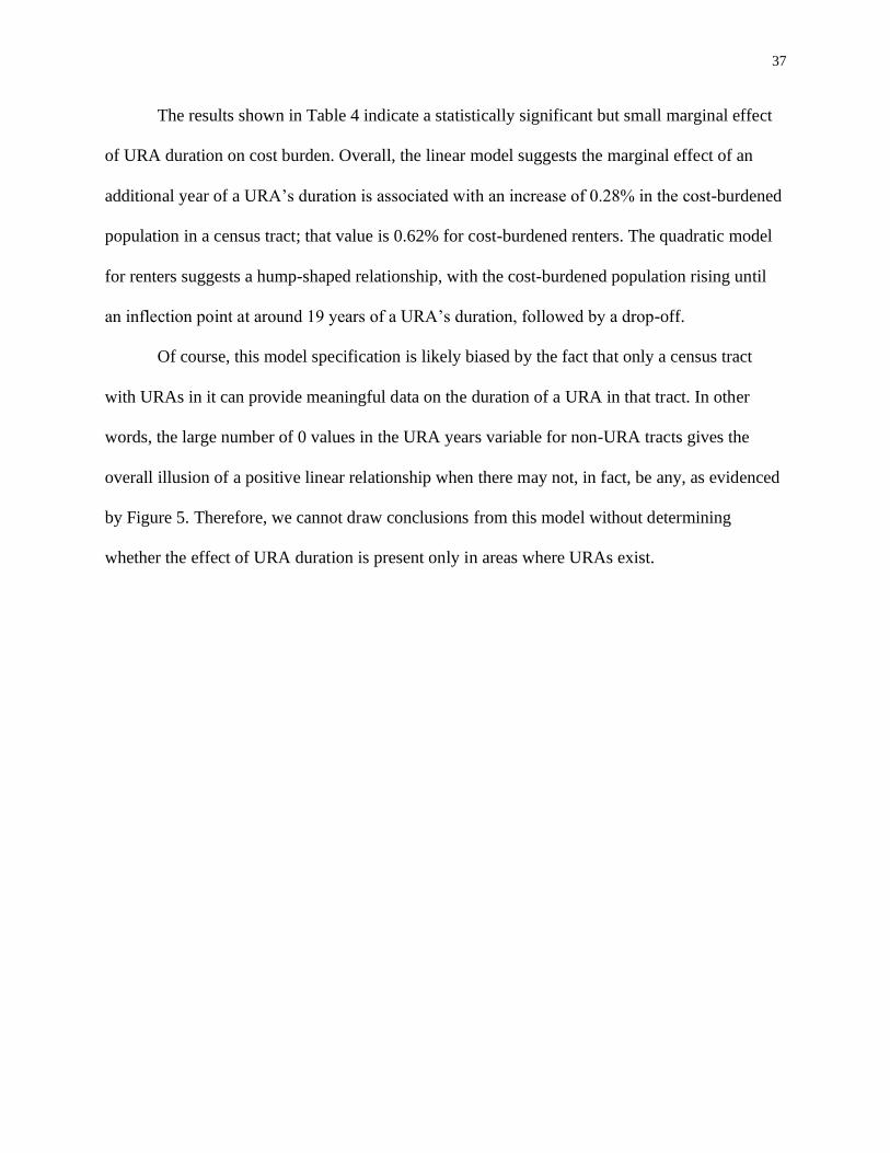
The results shown in Table 4 indicate a statistically significant but small marginal effect

of URA duration on cost burden. Overall, the linear model suggests the marginal effect of an

additional year of a URA’s duration is associated with an increase of 0.28% in the cost-burdened

population in a census tract; that value is 0.62% for cost-burdened renters. The quadratic model

for renters suggests a hump-shaped relationship, with the cost-burdened population rising until

an inflection point at around 19 years of a URA’s duration, followed by a drop-off.

Of course, this model specification is likely biased by the fact that only a census tract

with URAs in it can provide meaningful data on the duration of a URA in that tract. In other

words, the large number of 0 values in the URA years variable for non-URA tracts gives the

overall illusion of a positive linear relationship when there may not, in fact, be any, as evidenced

by Figure 5. Therefore, we cannot draw conclusions from this model without determining

whether the effect of URA duration is present only in areas where URAs exist.

38

Cost Burden (log)

VARIABLES Total Renters Homeowners

Years URA Existed 0.00274** (0.00127) 0.00519* (0.00290) 0.00622*** (0.00185) 0.0221*** (0.00436) 0.00216 (0.00174) 0.000663 (0.00462)

Years URA Existed2 -8.95e-05 (0.000104) -0.000581*** (0.000151) 5.48e-05 (0.000164)

Population (log) 0.897*** (0.0979) 0.899*** (0.0979) 1.638*** (0.163) 1.650*** (0.158) 0.409*** (0.123) 0.408*** (0.123)

Median Income (log) -0.521*** (0.0622) -0.524*** (0.0617) -1.198*** (0.102) -1.221*** (0.101) 0.0721 (0.0897) 0.0742 (0.0892)

Median Property Value in

$ (log)

0.0736** (0.0337) 0.0764** (0.0336) 0.0305 (0.0522) 0.0485 (0.0519) -0.00362 (0.0493) -0.00532 (0.0493)

Unemployment (%) -0.00586 (0.00420) -0.00605 (0.00421) -0.0204*** (0.00739) -0.0216*** (0.00722) 0.00450 (0.00583) 0.00461 (0.00584)

# on Public Assistance 0.000693*** (0.000263) 0.000695*** (0.000261) 0.00136*** (0.000504) 0.00137*** (0.000490) 0.000240 (0.000371) 0.000239 (0.000373)

Poverty (%) 0.00623** (0.00298) 0.00626** (0.00297) 0.00579 (0.00550) 0.00598 (0.00530) 0.00753** (0.00359) 0.00751** (0.00360)

Single Parents 0.000794*** (0.000151) 0.000788*** (0.000151) 0.00237*** (0.000269) 0.00233*** (0.000266) -0.000162 (0.000226) -0.000158 (0.000227)

College Education 0.000180*** (2.49e-05) 0.000181*** (2.49e-05) 0.000404*** (4.36e-05) 0.000414*** (4.30e-05) -8.21e-06 (3.33e-05) -9.13e-06 (3.35e-05)

Veterans -0.000367*** (0.000103) -0.000365*** (0.000102) -0.000574*** (0.000187) -0.000560*** (0.000186) -0.000140 (0.000152) -0.000142 (0.000152)

Disabled 5.28e-05 (6.59e-05) 5.37e-05 (6.58e-05) 4.10e-05 (0.000123) 4.67e-05 (0.000122) 6.12e-05 (9.69e-05) 6.06e-05 (9.71e-05)

Housing Stability -0.000130*** (2.40e-05) -0.000131*** (2.42e-05) -0.000294*** (3.85e-05) -0.000302*** (3.82e-05) -3.61e-06 (3.25e-05) -2.86e-06 (3.27e-05)

Non-English Speakers -1.54e-06 (3.16e-05) -1.61e-06 (3.15e-05) -1.92e-05 (5.19e-05) -1.97e-05 (5.14e-05) 9.27e-06 (4.07e-05) 9.31e-06 (4.09e-05)

Black pop. 0.000128* (7.29e-05) 0.000122 (7.45e-05) 7.88e-05 (0.000109) 3.52e-05 (0.000112) 0.000239** (0.000104) 0.000243** (0.000106)

Native American pop. -0.000338*** (0.000110) -0.000336*** (0.000110) -0.000533** (0.000250) -0.000517** (0.000251) -0.000262 (0.000200) -0.000263 (0.000201)

Hispanic pop. 4.03e-05 (3.23e-05) 4.00e-05 (3.20e-05) 6.76e-05 (5.74e-05) 6.61e-05 (5.59e-05) 5.37e-06 (3.78e-05) 5.52e-06 (3.79e-05)

New Housing 0.00112*** (0.000105) 0.00112*** (0.000105) -0.000161 (0.000231) -0.000172 (0.000231) 0.00169*** (0.000157) 0.00169*** (0.000157)

Share of renters (%) -0.00593*** (0.000867) -0.00591*** (0.000865) 0.00365*** (0.00118) 0.00376*** (0.00116) -0.0165*** (0.00115) -0.0165*** (0.00115)

Constant 4.219*** (1.199) 4.209*** (1.199) 5.198*** (1.800) 5.130*** (1.760) 2.036 (1.534) 2.043 (1.540)

Observations 813 813 813 813 813 813

R-squared 0.661 0.661 0.715 0.719 0.469 0.469

HC3 robust standard errors in parentheses *** p<0.01, ** p<0.05, * p<0.1

Table 4

39

The models in Table 5

restrict the sample to census tracts

that contain URAs (N=296).

Perhaps surprisingly, despite the

apparently strong association

between the existence of URAs and

cost-burdened households in the

overall sample, there does not

appear to be a statistically

significant relationship between

housing cost burdens and the

duration of a URA’s existence

(demonstrated graphically in

Figures 6 and 7). In other words,

the length of time that a URA has

existed appears to have no bearing

on the level of cost-burdened

households in a census tract that contains a URA. This is the case not only for overall

households, but for renters and homeowners as well. However, the sign on the coefficient for

total cost burden is positive, suggesting that there might be too much variation to isolate an

effect. Interestingly, the sign is negative for renters, suggesting a decrease in housing cost

burdens for renters over time, and positive for homeowners, suggesting an increase over time.

This might be consistent with increasing property values in URAs yielding higher costs for

Figure 6

Figure 7

40

homeowners in the form of property taxes. However, given the fact that none of these

coefficients are statistically significant, it is impossible to draw any strong conclusions from the

limited sample of census tracts that contain URAs. Nevertheless, these results reinforce the idea

that there must be some systematic difference between census tracts that contain URAs and those

that do not, so there must be another factor driving this difference.

41

Cost Burden (log)

VARIABLES Total Renters Homeowners

Years URA Existed 0.00155 (0.00203) 0.000780 (0.00577) -0.00272 (0.00275) -0.000441 (0.00751) 0.00461 (0.00304) 0.00133 (0.00952)

Years URA Existed2 2.11e-05 (0.000151) -6.24e-05 (0.000194) 8.99e-05 (0.000247)

Population (log) 0.746*** (0.171) 0.745*** (0.174) 1.107*** (0.246) 1.110*** (0.248) 0.405** (0.205) 0.401* (0.207)

Median Income (log) -0.441*** (0.119) -0.438*** (0.120) -0.960*** (0.149) -0.967*** (0.152) 0.0435 (0.169) 0.0536 (0.170)

Median Property Value in $ (log)

0.0601 (0.0498) 0.0596 (0.0498) 0.0959 (0.0746) 0.0973 (0.0743) -0.0641 (0.0694) -0.0662 (0.0703)

Unemployment (%) -0.00679 (0.00531) -0.00667 (0.00542) -0.00859 (0.00853) -0.00896 (0.00877) -0.00572 (0.00880) -0.00519 (0.00877)

# on Public Assistance 0.000801** (0.000333) 0.000802** (0.000333) 0.00173*** (0.000521) 0.00173*** (0.000523) 0.000502 (0.000551) 0.000507 (0.000552)

Poverty (%) 0.00864* (0.00459) 0.00864* (0.00460) 0.00759 (0.00685) 0.00759 (0.00687) 0.00614 (0.00563) 0.00614 (0.00563)

Single Parents 0.000362* (0.000215) 0.000362* (0.000216) 0.00124*** (0.000327) 0.00124*** (0.000329) -0.000134 (0.000360) -0.000133 (0.000362)

College Education 0.000189*** (3.99e-05) 0.000188*** (3.99e-05) 0.000387*** (5.64e-05) 0.000387*** (5.64e-05) 1.53e-05 (5.56e-05) 1.47e-05 (5.57e-05)

Veterans -0.000442*** (0.000147) -0.000441*** (0.000147) -0.000544** (0.000259) -0.000545** (0.000260) -0.000276 (0.000236) -0.000274 (0.000237)

Disabled 0.000176* (9.51e-05) 0.000176* (9.52e-05) 0.000191 (0.000145) 0.000192 (0.000145) 9.21e-05 (0.000141) 9.11e-05 (0.000141)

Housing Stability -9.99e-05** (3.93e-05) -9.97e-05** (3.96e-05) -0.000212*** (5.29e-05) -0.000213*** (5.30e-05) -9.63e-06 (5.36e-05) -8.73e-06 (5.39e-05)

Non-English Speakers 6.83e-05 (5.53e-05) 6.88e-05 (5.62e-05) 4.32e-06 (7.22e-05) 2.95e-06 (7.27e-05) 0.000148** (7.29e-05) 0.000150** (7.33e-05)

Black pop. -2.75e-05 (9.60e-05) -2.60e-05 (9.69e-05) -0.000171 (0.000129) -0.000176 (0.000130) 0.000121 (0.000161) 0.000128 (0.000162)

Native American pop. 0.000111 (0.000312) 0.000112 (0.000316) 0.000205 (0.000375) 0.000201 (0.000377) -0.000339 (0.000601) -0.000333 (0.000609)

Hispanic pop. -1.56e-05 (5.03e-05) -1.58e-05 (5.05e-05) 5.87e-05 (6.78e-05) 5.94e-05 (6.79e-05) -8.12e-05 (5.77e-05) -8.20e-05 (5.80e-05)

New Housing 0.000888*** (0.000160) 0.000887*** (0.000160) 0.000104 (0.000227) 0.000105 (0.000227) 0.00146*** (0.000273) 0.00146*** (0.000272)

Share of renters (%) -0.00602*** (0.00118) -0.00603*** (0.00117) 0.00346** (0.00165) 0.00350** (0.00165) -0.0201*** (0.00191) -0.0201*** (0.00190)

Constant 4.632** (2.223) 4.624** (2.224) 5.965** (2.724) 5.987** (2.729) 3.285 (2.835) 3.253 (2.841)

Observations 296 296 296 296 296 296

R-squared 0.676 0.676 0.719 0.719 0.541 0.541

HC3 robust standard errors in parentheses

*** p<0.01, ** p<0.05, * p<0.1

Table 5

42

Tertiary Findings

Despite my finding that the length of URA

duration does not appear to significantly change

the levels of cost burdened households, it is

possible that the forces of gentrification and

displacement manifest through other observable

characteristics. In order to further investigate the

possible influence of URAs over time, I attempted

to model the effect of URA duration on

alternative dependent variables that reflect

various operationalizations of gentrification and

displacement in the form of median income,

property value, and housing stability.3 Higher

property values and incomes alongside lower

housing stability would suggest that gentrification

is occurring, bringing wealthier newcomers while

displacing existing residents. Table 6 displays

these results while Figures 8, 9, and 10 portray

results graphically. In the cases of median income

and housing stability, the effect of URA duration

3 Preliminary auxiliary regressions yielded significantly lower levels of median income and property

value in census tracts with URAs, while no such relationship emerged for stability. These results are

printed in the Appendix.

Figure 8

Figure 9

Figure 10

43

took the form of a negative-sign quadratic curve, implying an initial increase followed by an

inflection point and a decrease. The inflection point for median income is 13 years, meaning that

census tracts with URAs that were established less than 13 years ago appear to have higher

median incomes, while tracts with older URAs appear to have lower median incomes. Similarly,

for housing stability, the inflection point is 10 years, meaning that census tracts with URAs that

were established less than 10 years ago appear to have higher levels of households that lived in

the same home one year prior, while tracts with older URAs have lower such levels. These

results are not necessarily indicative of gentrification, as there does not appear to be an influx of

new residents with higher incomes, but rather that incomes are rising for existing residents, at

least in areas with URAs that have existed for less than ten years. Interestingly, there does not

appear to be a significant relationship between URA duration and property values, which may

explain why cost burdens also do not appear to increase across the same dimension.

44

Table 6

Dependent Variable

VARIABLES Median Income (log) Median Property Value

in $ (log)

Housing Stability (log)

Years URA Existed 0.00704** (0.00353) -0.00660 (0.00799) 0.00309 (0.00257)

Years URA Existed2 -0.000267*** (9.13e-05) 0.000275 (0.000208) -0.000153** (6.69e-05)

Population (log) -0.158** (0.0656) -0.00655 (0.149) 0.754*** (0.0384)

Median Property Value

in $ (log)

0.00736 (0.0267) -0.0252 (0.0193)

Unemployment (%) -0.0170*** (0.00323) 0.00876 (0.00760) -0.00859*** (0.00245)

# on Public Assistance -0.000176 (0.000219) 1.89e-05 (0.000492) 0.000273* (0.000158)

Poverty (%) -0.0160*** (0.00178) -0.00616 (0.00453) 0.00484*** (0.00146)

Single Parents 6.62e-05 (0.000147) -0.000109 (0.000331) 0.000301*** (0.000101)

College Education 9.18e-05*** (2.08e-05) 0.000111** (4.79e-05) -4.21e-05*** (1.55e-05)

Veterans -0.000133 (9.80e-05) -0.000280 (0.000220) 0.000291*** (6.56e-05)

Disabled -0.000398*** (5.47e-05) 0.000193 (0.000134) 0.000110*** (4.22e-05)

Housing Stability 0.000127*** (1.87e-05) -1.05e-05 (4.53e-05)

Non-English Speakers -5.60e-05* (3.13e-05) -7.90e-05 (7.06e-05) 4.20e-05* (2.20e-05)

Black pop. 5.31e-05 (6.14e-05) 0.000300** (0.000137) -3.01e-05 (4.44e-05)

Native American pop. -3.28e-05 (0.000179) 0.000375 (0.000402) 3.32e-07 (0.000129)

Hispanic pop. 2.26e-06 (2.88e-05) 3.47e-05 (6.47e-05) 3.16e-05 (2.08e-05)

New Housing -0.000176* (9.19e-05) 0.000166 (0.000208) -7.46e-05 (6.67e-05)

Share of renters (%) -0.000961 (0.000638) -0.00440*** (0.00142) -0.00154*** (0.000453)

Median Income (log) 0.0372 (0.135) 0.342*** (0.0402)

Constant 12.21*** (0.584) 12.06*** (1.979) (0.563)

Observations 296 296 296

R-squared 0.777 0.146 0.934

HC3 robust standard errors in parentheses

*** p<0.01, ** p<0.05, * p<0.

45

V. Discussion

At first, this set of findings may seem to be muddled in its ability to determine whether

URAs are a driver of housing instability. It can be concluded that higher levels of cost-burdened

households seem to exist in census tracts with URAs, but it is unclear whether such high levels

preceded URAs in those areas or vice versa. Preliminary evidence points to lower incomes and

lower property values in these areas as well, which is consistent with URAs existing in blighted

areas with higher indicators of poverty and disinvestment. This seems to suggest that high cost

burdens are indicative of the type of area that would be a candidate for urban renewal, rather than

a consequence of it. If cost burdens were to increase alongside property values, that would be

evidence that urban renewal exacerbates the problem of housing-induced poverty as rising prices

force residents to devote a higher proportion of their income to cover housing costs. However,

within URAs, there is no evidence to suggest that either cost burdens or property values increase

with URA duration. This is generally in line with previous quantitative research that fail to find a

significant detrimental impact from gentrification on poor households (Freeman & Braconi,

2004; Vigdor, 2002). In this case, because property value inflation does not appear to be driving

up housing prices, households in these areas are not necessarily forced to choose between

moving away (being displaced) or staying put (becoming cost-burdened). However, it is

concerning that the disproportionately high cost burdens in these areas do not seem to change

across a URA’s duration. If urban renewal is designed as a tool to alleviate blight and improve

economic outcomes in an urban area, we might expect to see either a decrease in cost burdens as

the local economy improves, or an increase in cost burdens as a consequence of gentrification. A

lack of change signifies that there is persistent inequality and poverty in these areas in spite of

the economic development efforts that these urban renewal agencies are ostensibly pursuing.

46

This begs the question of whether there is any measurable economic effect of urban renewal as a

public policy tool, and whether it is effective in achieving its goals that are in the public interest.

The hump-shaped relationships between URA duration and both income and housing

stability do not seem to suggest that displacement is occurring as a result of gentrification.

Median incomes appear to increase along with URA duration up to the 13-year mark, while the

number of households reporting that they lived in the same home a year prior seems to increase

up to the 10-year mark. This may hint at the trajectory of economic development generated by

urban renewal. In the early years of an urban renewal district, new investment in the area appears

to yield higher incomes, while residents appear to enjoy increased housing stability, suggesting

that higher incomes are not being driven by newcomers. However, after ten years, housing

stability inverts as incomes continue to rise, although incomes eventually begin to decline as

well. It is possible that this time frame represents a limit to the effectiveness of urban renewal as

an economic development tool. In fact, it is not apparent that any long-run economic

improvements are occurring as a result of urban renewal, and that in fact it may be

counterproductive.

47

VI. Limitations

This study has numerous limitations that hinder any broader interpretation of its findings.

It assumes that urban renewal areas are static in each census tract, when in actuality urban

renewal agencies frequently amend their plans to annex or remove land from URAs. It also does

not account for any urban renewal areas that previously existed but were closed prior to 2018,

thus obscuring any effect those URAs may have had on the outcome variable. These coding

errors may have biased the results away from statistical significance and toward the null

hypothesis. Future research may be able to comprehensively map each urban renewal area onto a

census tract map using geographic information software, accounting for changes in land area

through time, which would more accurately capture the growth and changes of urban renewal

areas through the years. Also, this study does not account for categorical differences in the types

of urban renewal districts, as Weber et al. (2007) found that residential price effects are primarily

felt in mixed-use districts rather than commercial or industrial districts.

This study also uses imperfect operationalizations of the concepts of interest. Scholars

have pointed out the drawbacks of the cost-to-income ratio as a measurement of housing

insecurity, instead preferring the residual income approach which more precisely captures the

income dynamics of low-income households without distorting the preferences of households

with higher incomes. The concepts of gentrification and displacement are also imperfectly

proxied for using median income and the number of households who reported living in the same

home a year prior, which does not account for the reason for the move. It may be capturing both

in-movers and out-movers, muddying the separation between gentrification and displacement.

Ideally, displacement would represent households who decide to move away involuntarily or

become homeless, although these households are frequently unaccounted for in data systems.

48

Lastly, this study is a cross-sectional analysis using a single year’s worth of data, and

thus cannot accurately estimate the time effects that each URAs may actually create; instead, it

proxies for this time effect using the URA duration variable. However, a true time-series analysis

that uses many more observations could produce more accurate results that better model the

dynamics at work in these areas. For instance, a first-differences model might be able to capture

the rate at which property values are changing relative to inflation. A difference-in-differences

method could be employed to determine the before-and-after effects of urban renewal in cities

that adopted it. In particular, it would better clarify the question of whether high levels of cost

burden are present in areas before urban renewal is adopted. Alternatively, a two-stage

regression method such as that employed by Man and Rosentraub (1998) and Dye and Merriman

(2000) could resolve the self-selection problem of whether an area is likely to adopt urban

renewal.

49

VII. Conclusion

I find that census tracts that contain urban renewal areas have, on average, 5% higher

levels of cost-burdened households than census tracts without URAs, all else being equal.

Importantly, when separated by housing tenure, levels of housing cost burden for renters are 20%

higher in census tracts with URAs, while there appears to be no significant difference in the level

of cost-burdened homeowners.

Within census tracts that contain URAs, there appears to be no change in the levels of cost-

burdened households across the span of time that a URA exists, as census tracts with newer

URAs appear to have the same levels of cost-burdened households as those whose URAs have

existed longer. Additionally, median income and housing stability appear to increase in URAs

for a period of time (13 years and 10 years, respectively) before declining; property values do not

appear to significantly change across a URA’s duration.

The core finding from this study is that there seem to be disproportionately more cost-

burdened households in areas with URAs than those without, and cost burdens do not appear to

change across the duration of a URA’s existence. While we cannot definitively determine that

URAs are the cause of these higher cost burden levels, it is apparent that urban renewal does not

alleviate these high levels of housing instability either. In the current urban affordability crisis, it

is imperative that municipalities, particularly those that employ tax-increment financing as a

mechanism for urban renewal, leverage this awareness to achieve better housing affordability

outcomes for residents in blighted urban areas. One policy recommendation is for municipalities

to prioritize the construction of affordable housing rather than, or in addition to, business

development. This would demonstrate a city’s concern for its most vulnerable residents by using

this financing tool to repair persistent inequalities rather than benefiting owners of capital. If

50

local residents are concerned about the possibility of gentrification occurring in an area that is

identified for urban renewal, one option is to shift to neighborhood-driven management scheme

rather than central planning through the urban renewal agency. This empowers the residents in

neighborhood to decide on the priorities and developments that they believe will benefit the area

and avoids the impression that the city government is imposing its will without consent. Recent

examples of this model are Prosper Portland’s Neighborhood Prosperity Initiative

(Neighborhood Prosperity Initiative, 2020) and the South Corvallis Urban Renewal Plan as

organized by Living Southtown (Southtown Corvallis, 2020), although both of these examples

are only just beginning and their effectiveness will not be observable for several years hence.

Future research may continue to examine the role of urban renewal as a tool for economic

development as it continues to gain popularity among cities in Oregon.

51

References

Best Practices for Tax Increment Financing Agencies in Oregon. (2019). Oregon Economic

Development Association.

Brimmer, D., & Fitzgerald, T. (2019). Oregon Property Tax Statistics, Fiscal Year 2018-19 (No.

150-303-405 (Rev. 4-19); p. 74). Oregon Department of Revenue.

Brueckner, J. K. (2001). Tax increment financing: A theoretical inquiry. Journal of Public

Economics, 81(2), 321–343. https://doi.org/10.1016/S0047-2727(00)00123-7

Campos, L. (1979). The Portland Planning Commission: An Historical Overview. City of

Portland, Bureau of Planning.

Cox, R., Henwood, B., Rodnyansky, S., Rice, E., & Wenzel, S. (2019). Road map to a unified

measure of housing insecurity. Cityscape: A Journal of Policy Development and

Research •, 21(2), 93–127.

Cox, R., Rodnyansky, S., Henwood, B., & Wenzel, S. L. (2017). Measuring Population

Estimates of Housing Insecurity in the United States: A Comprehensive Approach. SSRN

Electronic Journal. https://doi.org/10.2139/ssrn.3086243

Dye, R. F., & Merriman, D. F. (2000). The Effects of Tax Increment Financing on Economic

Development. Journal of Urban Economics, 47(2), 306–328.

https://doi.org/10.1006/juec.1999.2149

Elsasser Watson, N., Steffen, B. L., Martin, M., & Vandenbroucke, D. A. (2017). Worst Case

Housing Needs 2017 Report to Congress (p. 92). U.S. Department of Housing and Urban

Development Office of Policy Development and Research.

Freeman, L. (2005). Displacement or Succession?: Residential Mobility in Gentrifying

Neighborhoods. Urban Affairs Review, 40(4), 463–491.

https://doi.org/10.1177/1078087404273341

Freeman, L., & Braconi, F. (2004). Gentrification and Displacement: New York City in the

1990s. Journal of the American Planning Association, 70(1), 39–52.

https://doi.org/10.1080/01944360408976337

Gibson, K. J. (2004). Urban redevelopment in Portland: Making the city livable for everyone? In

C. Ozawa (Ed.), The Portland Edge: Challenges and Successes in Growing Communities.

Island Press.

Glass, R. (2013). Aspects of Change. In J. Brown-Saracino (Ed.), The Gentrification Debates: A

Reader (pp. 19–27). Routledge.

52

Gotham, K. F. (2000). Growth Machine Up-Links: Urban Renewal and the Rise and Fall of a

Pro-Growth Coalition in a U.S. City. Critical Sociology, 26(3), 268–300.

https://doi.org/10.1177/08969205000260030501

Gotham, K. F. (2001). A City without Slums: Urban Renewal, Public Housing, and Downtown

Revitalization in Kansas City, Missouri. The American Journal of Economics and

Sociology, 60(1), 285–316. JSTOR.

Hampson, R. (2005, April 20). Studies: Gentrification a boost for everyone. USA Today, 13A-

14A.

Hoffman, A. von. (2000). A study in contradictions: The origins and legacy of the housing act of

1949. Housing Policy Debate, 11(2), 299–326.

https://doi.org/10.1080/10511482.2000.9521370

Hughes, J. (2019). Historical Context of Racist Planning: A History of How Planning Segregated

Portland (p. 32). Bureau of Planning and Sustainability, City of Portland.

Hyra, D. (2015). The back-to-the-city movement: Neighbourhood redevelopment and processes

of political and cultural displacement. Urban Studies, 52(10), 1753–1773.

https://doi.org/10.1177/0042098014539403

Kutty, N. K. (2005). A new measure of housing affordability: Estimates and analytical results.

Housing Policy Debate, 16(1), 113–142. https://doi.org/10.1080/10511482.2005.9521536

Luque, J. (2020). Assessing the role of TIF and LIHTC in an equilibrium model of affordable

housing development. Regional Science and Urban Economics, 80, 103377.

https://doi.org/10.1016/j.regsciurbeco.2018.06.005

Man, J. Y., & Rosentraub, M. S. (1998). Tax Increment Financing: Municipal Adoption and

Effects On Property Value Growth. Public Finance Review, 26(6), 523–547.

https://doi.org/10.1177/109114219802600601

Martin, I. W., & Beck, K. (2018). Gentrification, Property Tax Limitation, and Displacement.

Urban Affairs Review, 54(1), 33–73. https://doi.org/10.1177/1078087416666959

Neighborhood Prosperity Initiative. (2020). Prosper Portland.

https://prosperportland.us/neighborhood-prosperity-initiative/

Newman, K., & Wyly, E. K. (2006). The Right to Stay Put, Revisited: Gentrification and

Resistance to Displacement in New York City. Urban Studies, 43(1), 23–57.

https://doi.org/10.1080/00420980500388710

Schwartz, M., & Wilson, E. (2008). Who Can Afford To Live in a Home?: A look at data from

the 2006 American Community Survey (p. 13). U. S. Census Bureau.

53

Slater, T. (2009). Missing Marcuse: On gentrification and displacement. City, 13(2–3), 292–311.

https://doi.org/10.1080/13604810902982250

Southtown Corvallis. (2020). http://devnw.org/thriving-communities/community-building-and-

neighborhood-revitalization/southtown-corvallis/

Stone, M. E. (2004). Shelter Poverty: The Chronic Crisis of Housing Affordability. New England

Journal of Public Policy, 20(1), 107–119.

Stone, M. E. (2010). What is housing affordability? The case for the residual income approach.

Housing Policy Debate.

http://www.tandfonline.com/doi/abs/10.1080/10511482.2006.9521564

Stone, M. E. (2010). Shelter Poverty: New Ideas on Housing Affordability. Temple University

Press.

Tax Increment Finance Best Practices Reference Guide. (2007). Council of Development

Finance Agencies and International Council of Shopping Centers.

Thalmann, P. (1999). Identifying Households which Need Housing Assistance. Urban Studies,

36(11), 1933–1947. https://doi.org/10.1080/0042098992683

Vigdor, J. L. (2002). Does Gentrification Harm the Poor? Brookings-Wharton Papers on Urban

Affairs, 133–182. JSTOR.

Weber, R., Bhatta, S. D., & Merriman, D. (2007). Spillovers from tax increment financing

districts: Implications for housing price appreciation. Regional Science and Urban

Economics, 37(2), 259–281. https://doi.org/10.1016/j.regsciurbeco.2006.11.003

Wetzstein, S. (2017). The global urban housing affordability crisis. Urban Studies, 54(14), 3159–

3177. https://doi.org/10.1177/0042098017711649

Wollner, C., Provo, J., & Schablitsky, J. (2001). A Brief History of Urban Renewal in Portland,

Oregon (AF/165431; p. 56). Portland Development Commission.

Wyly, E., Newman, K., Schafran, A., & Lee, E. (2010). Displacing New York. Environment and

Planning A: Economy and Space, 42(11), 2602–2623. https://doi.org/10.1068/a42519

54

Appendices

55

Appendix A: Urban Renewal Areas in Oregon

Agency Plan Area County Census Tracts Year Established

Years Since

Establishment (as of 2018)

City of Philomath Philomath UR Plan Area Benton 108 1990 28

City of Estacada Estacada Plan Area Clackamas 242 2007 11

Clackamas County N Clackamas Revitalization UR Plan Area Clackamas 210, 211, 216.01, 216.02 2006 12

City of Gladstone Gladstone 1 UR Plan Area Clackamas 217, 219, 220, 221.01, 221.08 1988 30

City of Lake Oswego East End Lake Oswego UR Plan Area Clackamas 202 1986 32

City of Lake Oswego Lake Grove Village Center UR Plan Area Clackamas 203.02, 203.03, 204.01, 202 2012 6

City of Oregon City Oregon City Downtown/N. End UR Plan Area Clackamas 225, 224, 223.01, 223.02 1990 28

City of Wilsonville Wilsonville Yr2000 UR Plan Area Clackamas 227.08, 227.07, 227.10, 244 1990 28

City of Wilsonville Wilsonville West Side UR Plan Area Clackamas 227.07 2003 15

City of Wilsonville Coffee Creek UR Plan Area Washington 321.1 2016 2

City of Sandy Sandy UR Plan Area Clackamas 234.01, 234.03, 234.04, 243.02 1998 20

City of Canby Canby UR Plan Area Clackamas 229.01, 229.06, 229.07, 229.04, 1999 19

City of Molalla Molalla UR Plan Area Clackamas 239.01, 239.02, 238 2008 10

City of Milwaukie Milwaukie UR Plan Area Clackamas 206, 212, 214, 211, 209 2016 2

City of Astoria Astoria East UR Plan Area Clatsop 9502, 9503 1980 38

City of Astoria Astoria West UR Plan Area Clatsop 9501, 9502 2002 16

City of Seaside South East Seaside Plan Area Clatsop 9509, 9511 2017 1

City of Warrenton Warrenton UR Plan Area Clatsop 9505, 9506 2007 11

City of Rainier Rainier Waterfront UR Plan Area Columbia 9703 1993 25

Columbia County Port Westward UR Plan Area Columbia 9702 2001 17

City of St Helens St Helens UR Plan Area Columbia 9706, 9707, 9708 2017 1

Coos County Coos County North Bay UR Plan Area Coos 5.02, 5.03, 5.04, 4, 1 1986 32

City of Bandon Bandon 1 UR Plan Area Coos 10 1987 31

City of Bandon Bandon 2 UR Plan Area Coos 10 1990 28

Table A1

56

City of Coos Bay Coos Bay Downtown UR Plan Area Coos 7 1988 30

City of Coos Bay Coos Bay Empire UR Plan Area Coos 5.03, 5.04 1995 23

City of North Bend North Bend Downtown UR Plan Area Coos 3, 4 1994 24

City of Coquille Coquille UR Plan Area Coos 9 1998 20

City of Brookings Brookings Downtown UR Plan Area Curry 9503.01, 9503.02 2002 16

City of Gold Beach City of Gold Beach Urban Renewal Area Curry 9502 2013 5

City of Redmond Redmond Downtown UR Plan Area Deschutes 8, 9 1995 23

City of Bend Bend Juniper Ridge UR Plan Area Deschutes 11, 12 2005 13

City of Bend Murphy Crossing UR Plan Area Deschutes 20, 21 2008 10

City of Sisters Sisters Downtown UR Plan Area Deschutes 5 2003 15

City of La Pine La Pine UR Plan Area Deschutes 2 2014 4

City of Roseburg North Roseburg UR Plan Area Douglas 800, 900, 1200, 1300 1989 29

City of Winston Winston Division UR Plan Area Douglas 1600 2006 12

City of Reedsport Reedsport Urban Renewal Division Douglas 100 2007 11

City of Hood River Columbia Cascade/H.R. UR Plan Area Hood River 9503 1987 31

City of Hood River Waterfront UR Plan Area Hood River 9503 2008 10

City of Hood River Hood River Heights Business District Hood River 9503 2011 7

Hood River County Windmaster UR Plan Area Hood River 9502 2007 11

City of Medford Medford City Center UR Plan Area Jackson 1, 16.01, 2.01, 2.02 1988 30

City of Talent Talent UR Plan Area Jackson 17 1991 27

City of Jacksonville Jacksonville UR Plan Area Jackson 15 2002 16

City of Phoenix Phoenix UR Plan Area Jackson 16.01, 16.02, 6.02, 24 2005 13

City of Central Point

Downtown & East Pine Street Corridor

Revitalization Plan Jackson 9, 10.01, 10.02, 11 2011 7

City of Culver City Of Culver UR Plan Area Jefferson 9603.02 2007 11

City of Madras Madras City UR Plan Area Jefferson 9602.01, 9602.02 2005 13

City of Grants Pass Grants Pass Urban Renewal Plan Area Josephine 3611, 3612, 3607.02, 3607.01, 3605, 3606, 3604 2016 2

City of Klamath Falls Klamath Town Center UR Plan Area Klamath 9716, 9715, 9712 2005 13

City of Klamath Falls Lakefront UR Plan Area Klamath 9718 2001 17

City of Klamath Falls Spring Street UR Plan Area Klamath 9718, 9719 2017 1

57

City of Eugene Eugene Downtown UR Plan Area Lane 39 1968 50

City of Eugene Riverfront UR Plan Area Lane 37, 38, 39, 40 1985 33

City of Veneta Veneta Downtown UR Plan Area Lane 9.03, 9.04 1984 34

City of Coburg Coburg Industrial Park UR Plan Area Lane 3 2001 17

City of Springfield

(SED) Glenwood UR Plan Area Lane 36, 17 2004 14 City of Springfield

(SED) Springfield Downtown UR Plan Area Lane 32.02, 33.02, 34 2007 11

City of Florence Florence UR Plan Area Lane 7.05, 7.07 2006 12

City of Waldport Waldport 2 UR Plan Area Lincoln 9516 2005 13

City of Lincoln City Lincoln City Yr2000 UR Plan Area Lincoln 9506.01, 9504, 9503.04, 9503.03 1988 30

City of Newport Newport South Beach UR Plan Area Lincoln 9512 1983 35

City of Newport Mclean Point Plan Area Lincoln 9511 2015 3

City of Newport Northside Plan Area Lincoln 9510, 9511, 9509, 9508 2015 3

City of Yachats Yachats UR Plan Area Lincoln 9517 2006 12

City of Depoe Bay Depoe Bay Plan Area Lincoln 9506.02 2008 10

City of Lebanon NW Lebanon 2 UR Plan Area Linn 308 1989 29

City of Lebanon Lebanon 3 UR Plan Area Linn 309.04 2000 18

City of Lebanon North Gateway UR Plan Area Linn 308 2008 10

City of Harrisburg Harrisburg UR Plan Area Linn 306 1992 26

City of Albany Central Albany UR Plan Area Linn 203, 204, 208.01, 208.02 2001 17

City of Salem Mcgilchrist UR Plan Area Marion 10 2006 12

City of Salem Riverfront/Downtown UR Plan Area Marion 2, 3 1975 43

City of Salem Mill Creek UR Plan Area Marion 18.03, 20, 10, 27 2005 13

City of Salem South Waterfront UR Plan Area Marion 12, 13, 2 2007 11

City of Salem North Gateway UR Plan Area Marion 3, 5.01, 4, 5.02, 16.01 1990 28

City of Salem West Salem UR Plan Area Polk 51, 52.02 2001 17

City of Woodburn Woodburn UR Plan Area Marion 103.06, 103.07, 103.04, 103.05, 103.03 2001 17

City of Silverton Silverton UR Plan Area Marion 105.03, 105.02 2004 14

City of Boardman Central Boardman UR Plan Area Morrow 9701 2008 10

58

City of Boardman West Boardman UR Plan Area Morrow 9701 2013 5

City of Portland (PP) Downtown UR Plan Area Multnomah 51, 106, 57 1984 34

City of Portland (PP) 42nd Avenue UR Plan Multnomah 36.03, 74, 30, 75 2012 6

City of Portland (PP) Cully Blvd UR Plan Multnomah 74, 75, 76, 28.01, 29.01 2012 6

City of Portland (PP) Parkrose UR Plan Multnomah 77, 78, 79 2012 6

City of Portland (PP) 82nd & Division UR Plan Multnomah 16.01, 16.02, 7.01, 83.01 2012 6

City of Portland (PP) Division-Midway UR Plan Multnomah 82.02, 84, 92.01, 90, 92.02, 91.01, 97.01 2012 6

City of Portland (PP) Rosewood UR Plan Multnomah 92.01, 92.02, 97.01, 93.01, 97.02, 96.05, 96.06 2012 6

City of Portland (PP) South Park Blocks UR Plan Area Multnomah 52, 106 1985 33

City of Portland (PP) Central East Side UR Plan Area Multnomah 21, 11.01, 11.02, 10 1986 32

City of Portland (PP) Airport Way UR Plan Area Multnomah 73 1986 32

City of Portland (PP) Convention Center UR Plan Area Multnomah 23.03, 24.02 1989 29

City of Portland (PP) Lents Town Center UR Plan Area Multnomah

8.02, 7.02, 4.02, 5.01, 5.02, 83.01, 83.02, 6.01, 6.02, 85, 84, 90,

89.02, 86 1998 20

City of Portland (PP) River District UR Plan Area Multnomah 45, 50, 51 1998 20

City of Portland (PP) Macadam UR Plan Area Multnomah 56, 57, 59 1999 19

City of Portland (PP) N Interstate Corridor UR Plan Area Multnomah

72.01, 72.02, 38.01, 39.01, 40.01, 40.02, 41.02, 42, 38.02,

39.02, 36.01, 38.03, 37.02, 35.01, 9800, 34.01, 33.01, 32, 31,

35.02, 34.02, 22.03 2000 18

City of Portland (PP) Gateway UR Plan Area Multnomah 80.01, 80.02, 81, 82.01, 82.02 2001 17

City of Gresham

(GRC) Rockwood/W Gresham UR Plan Area Multnomah 102, 96.05, 96.04, 96.03, 96.06, 93.01, 97.02, 98.01, 101 2003 15

City of Troutdale Troutdale Riverfront UR Plan Area Multnomah 103.05 2006 12

City of Wood Village Wood Village UR Plan Area Multnomah 103.04, 103.03 2010 8

City of Independence Independence UR Plan Area Polk 203.02 2008 10

City of Dallas Dallas UR Plan Area Polk 202.03, 205, 202.02 2005 13

City of Monmouth Monmouth UR Plan Area Polk 203.03, 203.04 2005 13

City of Garibaldi Garibaldi UR Plan Area Tillamook 9602 2006 12

City of Tillamook Tillamook UR Plan Area Tillamook 9604, 9605 2006 12

City of Pendleton Pendleton UR Plan Area Umatilla 9506, 9507 2003 15

City of Hermiston Hermiston UR Plan Area Umatilla 9510, 9511, 9512 2013 5

City of La Grande La Grande UR Plan Area Union 9704, 9705, 9706, 9707, 9708 1999 19

59

City of The Dalles Columbia Gateway Downtown UR Plan Area Wasco 9702, 9704 1990 28

City of Sherwood Old Town UR Plan Area Washington 322, 321.03, 321.04 2000 18

City of North Plains North Plains UR Plan Area Washington 327 2006 12

City of Tigard Tigard UR Plan Area Washington 306, 309, 319.12, 308.01, 307 2006 12

City of Tigard Tigard Triangle Urban Renewal Plan Washington 306, 307 2017 1

City of Hillsboro North Hillsboro UR Plan Area Washington 326.03, 326.07 2015 3

City of Hillsboro Downtown Hillsboro UR Plan Area Washington 325.01, 324.10, 324.09, 326.06, 326.04, 326.03 2009 9

City of Beaverton Central Beaverton UR Plan Area Washington 311, 312, 304.01, 313, 314.02, 314.04, 302 2011 7

City of Forest Grove Forest Grove UR Plan Area Washington 331.01, 331.02, 332, 333.01 2014 4

City of Banks Banks Urban Renewal Plan Area Washington 335 2017 1

City of Carlton Carlton UR Plan Area Yamhill 304 2009 9

City of McMinnville McMinnville UR Plan Area Yamhill 307.01, 308.01, 306.01 2013 5

City of Dundee Dundee UR Plan Area Yamhill 303.01 2017 1

60

Appendix B: Percentage Point Regression Results

Cost Burden (%)

VARIABLES Renters Homeowners

With Mortgage

Homeowners

Without Mortgage

URA 1.268 (0.917) 0.396 (0.742) 0.729 (0.695)

Population (log) 2.872*** (1.050) 0.0798 (0.850) 1.066 (0.796)

Median Income (log) -17.64*** (2.548) -7.047*** (2.063) 0.620 (1.933)

Median Property Value in

$ (log)

-0.464 (1.185) 1.581* (0.959) -1.708* (0.899)

Unemployment (%) 0.0202 (0.156) 0.136 (0.126) -0.235** (0.118)

# on Public Assistance (%) 0.461** (0.202) 0.168 (0.164) 0.0456 (0.154)

Poverty (%) 0.242** (0.102) -0.0119 (0.0823) 0.134* (0.0771)

Single Parents (%) 0.266** (0.130) 0.00666 (0.105) -0.00194 (0.0987)

College Education (%) 0.152*** (0.0432) -0.0456 (0.0349) 0.00836 (0.0327)

Veterans (%) -0.0516 (0.174) -0.0540 (0.141) -0.147 (0.132)

Disabled (%) -0.261* (0.134) -0.213* (0.109) 0.199* (0.102)

Housing Stability (%) 0.194*** (0.0712) 0.120** (0.0577) -0.0334 (0.0540)

Non-English Speakers (%) 0.0890 (0.0736) 0.0441 (0.0596) -0.0127 (0.0558)

Black pop. (%) 0.00446 (0.155) 0.197 (0.125) 0.515*** (0.117)

Native American pop. (%) -0.668*** (0.215) -0.203 (0.174) -0.171 (0.163)

Hispanic pop. (%) -0.204** (0.0791) -0.109* (0.0640) -0.0189 (0.0600)

New Housing (%) -0.0591 (0.101) 0.159* (0.0815) -0.0530 (0.0764)

Share of renters (%) -0.0363 (0.0254) 0.0576*** (0.0206) -0.00577 (0.0193)

Constant 205.8*** (30.59) 90.14*** (24.77) 20.97 (23.21)

Observations 813 813 813

R-squared 0.210 0.079 0.074

Standard errors in parentheses

*** p<0.01, ** p<0.05, * p<0.1

Table A2

61

Appendix C: Negative Binomial Regression Results

Cost Burden

VARIABLES Total Renters Homeowners

URA 0.0472** (0.0221) 0.154*** (0.0336) 0.0164 (0.0305)

Population (log) 0.862*** (0.0722) 1.569*** (0.114) 0.375*** (0.100)

Median Income (log) -0.537*** (0.0552) -1.175*** (0.0866) 0.0366 (0.0767)

Median Property Value in

$ (log)

0.0705** (0.0291) 0.0584 (0.0435) -0.0151 (0.0412)

Unemployment (%) -0.00522 (0.00383) -0.0205*** (0.00598) 0.00718 (0.00523)

# on Public Assistance 0.000575** (0.000237) 0.00117*** (0.000372) 0.000121 (0.000329)

Poverty (%) 0.00458* (0.00246) 0.00331 (0.00387) 0.00659** (0.00335)

Single Parents 0.000752*** (0.000157) 0.00215*** (0.000240) -0.000150 (0.000219)

College Education 0.000172*** (2.29e-05) 0.000374*** (3.63e-05) -7.01e-06 (3.12e-05)

Veterans -0.000326*** (0.000103) -0.000548*** (0.000156) -9.79e-05 (0.000144)

Disabled 3.97e-05 (6.56e-05) 3.75e-05 (1.00e-04) 2.12e-05 (9.08e-05)

Housing Stability -0.000124*** (2.13e-05) -0.000270*** (3.22e-05) 4.31e-06 (2.96e-05)

Non-English Speakers -3.69e-07 (3.18e-05) -1.22e-05 (4.91e-05) -3.47e-06 (4.35e-05)

Black pop. 0.000148** (7.47e-05) 7.76e-05 (0.000115) 0.000249** (0.000101)

Native American pop. -0.000321** (0.000133) -0.000488** (0.000203) -0.000242 (0.000180)

Hispanic pop. 4.00e-05 (3.12e-05) 5.39e-05 (4.92e-05) -6.09e-07 (4.22e-05)

New Housing 0.00110*** (0.000101) -0.000104 (0.000153) 0.00166*** (0.000140)

Share of renters (%) -0.00536*** (0.000647) 0.00404*** (0.000970) -0.0157*** (0.000929)

ln(alpha) -2.489*** (0.0502) -1.639*** (0.0501) -1.852*** (0.0496)

Constant 4.749*** (0.952) 5.236*** (1.499) 2.899** (1.305)

Observations 813 813 813

Standard errors in parentheses

*** p<0.01, ** p<0.05, * p<0.1

Table A3

62

Appendix D: Auxiliary Regression Results

Dependent Variable

VARIABLES Median Income (log) Median Property Value

in $ (log)

Housing Stability (log)

URA -0.0292** (0.0137) -0.0597** (0.0290) -0.0129 (0.00897)

Population (log) -0.255*** (0.0645) -0.0222 (0.0866) 0.824*** (0.0574)

Property Value in

$ (log)

0.0452** (0.0204) -0.0277*** (0.0102)

Unemployment (%) -0.0137*** (0.00266) 0.0115** (0.00455) -0.00385 (0.00345)

# on Public Assistance 6.61e-05 (0.000131) 0.000296 (0.000302) 5.77e-05 (0.000136)

Poverty (%) -0.0193*** (0.00162) -0.00504* (0.00273) 0.00235 (0.00275)

Single Parents -4.51e-05 (0.000103) -0.000112 (0.000182) 0.000332*** (8.31e-05)

College Education 6.60e-05*** (1.89e-05) 0.000134*** (2.82e-05) -4.17e-05*** (1.15e-05)

Veterans -6.30e-05 (6.15e-05) -0.000134 (0.000143) 0.000204*** (5.38e-05)

Disabled -0.000445*** (3.68e-05) 0.000176** (8.37e-05) 0.000105*** (3.13e-05)

Housing Stability 0.000146*** (1.74e-05) -3.85e-05 (2.44e-05)

Non-English Speakers -2.28e-06 (2.92e-05) -4.44e-05 (3.09e-05) 3.35e-05*** (1.23e-05)

Black pop. 3.69e-05 (4.42e-05) 0.000199*** (6.96e-05) -3.59e-05 (3.13e-05)

Native American pop. 7.43e-05 (6.16e-05) -7.96e-05 (0.000130) 3.03e-05 (3.69e-05)

Hispanic pop. -3.46e-05 (2.36e-05) 1.92e-05 (3.05e-05) 2.39e-05* (1.33e-05)

New Housing -5.21e-05 (6.37e-05) 0.000247** (0.000114) -7.41e-05* (4.43e-05)

Share of renters (%) -0.000974** (0.000465) -0.00402*** (0.000807) -0.000860*** (0.000249)

Median Income (log) 0.163** (0.0743) 0.315*** (0.0313)

Constant 12.53*** (0.542) 10.86*** (1.169) -1.820*** (0.415)

Observations 813 813 813

R-squared 0.730 0.174 0.940

HC3 robust standard errors in parentheses

*** p<0.01, ** p<0.05, * p<0.1

Table A4