ABSTRACT

MOHAN, SIBIN. Exploiting Hardware/Software Interactionsfor Analyzing Embedded Systems.(Under the direction of Associate Professor Frank Mueller).

Embedded systems are often subject to real-time timing constraints. Such systems require

determinism to ensure that task deadlines are met. The knowledge of the bounds on worst-case

execution times (WCET) of tasks is a critical piece of information required to achieve this objective.

One limiting factor in designing real-time systems is theclass of processorsthat may

be used. Contemporary processors with their advanced architectural features, such as out-of-order

execution, branch prediction, speculation, and prefetching, cannot be statically analyzed to obtain

WCETs for tasks as they introduce non-determinism into taskexecution, which can only be resolved

at run-time. Such micro-processors are tuned to reduce average-case execution times at the expense

of predictability. Hence, they do not find use in hard real-time systems. On the other hand, static

timing analysis derives bounds on WCETs but requires thatbounds on loop iterations be known

statically, i.e., at compile time. This limits the class of applications thatmay be analyzed by static

timing analysis and, hence, used in a real-time system. Finally, many embedded systems have com-

munication and/or synchronization constructs and need to function on a wide spectrum of hardware

devices ranging from small microcontrollers to modern multi-core architectures. Hence, anysin-

gle analysis technique (be it static or dynamic) will not suffice in gauging the true nature of such

systems.

This thesis contributesnovel techniques that use combinations of analysis methodsand

constant interactions between them to tackle complexitiesin modern embedded systems. To be more

specific, this thesis

(I) introduces of a new paradigm that proposes minor enhancements to modern processor architec-

tures, which, on interaction with software modules, is ableto obtain tight, accurate timing analysis

results for modern processors;

(II) it shows how the constraint concerning statically bound loops may be relaxed and applied to

make dynamic decisions at run-time to achieve power savings;

(III) it represents the temporal behavior of distributed real-time applications as colored graphs cou-

pled with graph reductions/transformations that attempt to capture inherent “meaning” in the appli-

cation.

To the best of my knowledge, these methods that utilize interactions between different

sources of information to analyze modern embedded systems are a first of their kind.

Exploiting Hardware/Software Interactions for AnalyzingEmbedded Systems

bySibin Mohan

A dissertation submitted to the Graduate Faculty ofNorth Carolina State University

in partial fullfillment of therequirements for the Degree of

Doctor of Philosophy

Computer Science

Raleigh, North Carolina

2008

APPROVED BY:

Dr. Alex Dean Dr. Purush Iyer

Dr. Frank Mueller Dr. Tao XieChair of Advisory Committee

ii

DEDICATION

to ammumma, mom, dad and rads

iii

BIOGRAPHY

Sibin Mohan was born on March 20, 1979 to Mrs. T. Shobhana and Mr. B. M. C. Kumar

in Kozhikode (Kerala, India), but has lived mostly in the lovely city that is Bangalore. He completed

his schooling at the Frank Anthony Public School (FAPS), Bangalore. He received his Bachelor of

Engineering (B.E.) undergraduate degree in Computer Science and Engineering from PES Institute

of Technology which is a part of Bangalore University, India. He then worked at Hewlett-Packard

India Software Operations, Bangalore, as a Software Engineer for one year.

Sibin joined the graduate program in the Dept. of Computer Science at North Carolina

State University in Fall 2002 where he has been since, working with Dr. Frank Mueller. He obtained

his Masters degree in Computer Science in Fall 2004. Sibin isthe recipient of the “Preparing the

Professoriate” fellowship from the Graduate School at North Carolina State University. Since Fall

2004 he has been pursuing his Ph.D. in Computer Science at North Carolina State University, mainly

in the Systems area.

iv

ACKNOWLEDGMENTS

This dissertation is the culmination of many years of work, all of which have been ex-

tremely rewarding. I have been able to reach this goal largely due to the belief, support and wisdom

imparted by many people I have had the honour of interacting with over the years. While I try to

acknowledge every single one of them, I realize that being only human, I might miss a few names.

To Dr. Frank Mueller, my advisor, I offer sincere thanks and appreciation for having the

patience to shepherd me through the journey that was this Ph.D. As the ancient Chinese proverb

states, “a journey of a thousand miles begins with a single step.” I realize that this Ph.D., that first

important step, would not have been possible without his insight, advice, critique and support. His

counsel on research methodology, teaching, presentation skills, writing skills, etc. have all been

instrumental in shaping me as a researcher. His management style, dedication towards research and

attention to detail is something that I can only hope to emulate. He has also guided and actively

assisted me through the long process of searching for futurecareer opportunities.

Some of the best courses I took during my time at NC State was courtesy of Dr. Matt

Stallmann. His courses challenged and excited me at the sametime and often made me see the field

of Computer Science in a new light. He was also gracious enough to mentor me through the process

of navigating my way through my first comprehensive teachingassignment.

Comments and questions raised by Dr. Alex Dean, Dr. Purush Iyer and Dr. Tao Xie

helped me focus on important issues and avoid pitfalls during the course of my research. I would

like to thank them for being a part of my dissertation committee and guidance provided thus.

Dr. Purush Iyer, Dr. Peng Ning, Dr. Nagiza Samatova and Dr. Tao Xie took time off their

busy schedules to examine and provide valuable feedback on my job application materials. I am

thankful for their feedback and the knowledge that they imparted during the whole process. I am

also grateful to Dr. Becky Rufty for her valuable advice on this and related topics. I would also like

to thank Dr. David Whalley and Dr. John Regehr for writing reference letters for me.

I would also like to thank Dr. Eric Rotenberg as many of the ideas in this dissertation

would not have come up if not for the deep understanding of computer architecture he instilled in

me via his courses. I would also like to thank him for making his architecture simulator and toolset

available for use in my research. Aravind Anantaraman and Vimal Reddy were always willing to

help me to understand and solve problems related to the simulator framework and for that I am

grateful.

Graduate school can never be complete or pleasant without the administration that silently

v

moves the great machinery in the background. Dr. David Thuente as the Director of Graduate

Programs has been very helpful in directing me through the administrative details that go along

with being a student. I would also like to thank the Computer Science staff members, Margery

Page, Carol Allen, Ginny King and Susan Peaslee, to name but afew.

Not a day goes by that I don’t remember, or feel grateful towards, Mr. Vijayan. His teach-

ings on C++, programming paradigms, operating systems,etc. coupled with quick philosophical

insights often drew parallels with slices of real life. I attempt to emulate his remarkable teaching

style every time I step in front of a classroom full of students. I would also like to thank Dr. Krishna

Rao and Mr. Joye Joseph whose teaching had a profound effect on me.

Johannes Helander took a chance on a graduate student he met at a conference and has

been a mentor and friend ever since. That was the start of a great opportunity for me; an opportunity

to work on some really exciting research ideas. Conversations with him range over a diversity of

topics, from cutting-edge research ideas to varieties of beer, all of which ensures that every time I

talk to him I come back having learned something new.

Jaydeep, Nirmit, Yifan, Kaustubh, Kiran, Anita, Harini, Anubhav, Nik, Ravi, Chao, Arun,

Vivek, Raghuveer and Heshan have all been great lab-mates over the years. Interactions with them

resulted in my learning a great deal and often made me look forward to coming in to work every

day. I would also like to thank my various room-mates (Salil,Ajit, Rahul, Ishdeep, Sharath) who

have had to put up with me and my cooking over the years!

No person is complete without his friends and I consider myself lucky to have some

amazing people as close friends. Nisha, whose thought processes resemble mine in uncanny ways,

provides a mirror to the inner workings of my mind. I considermyself lucky to have her alongside

as one of my closest friends, right from our childhood days. Ayush, Biju, Chatt, Cherry, David,

Ramesh and Palani ensured that school and everything else that followed was memorable. Meeting

and/or talking to them is still something I eagerly look forward to. Cohan, always has the ability to

surprise me, albeit in a pleasant way. He is brimming with ideas that he loves to share, is extremely

helpful and is one of the nicest, smartest and best read people I have come across. Mrin, Sudheer,

Chinmoyee and their family ensured that I never missed home and were always ready to welcome

me into their family moments. Hema, a very dear friend, was the first person to take the effort to

instruct me on the meaning of my own name. She is a terrific companion for attending concerts,

reminiscing about bygone days, you name it. Folks that I met while working in various voluntary

organizations on campus have also helped me achieve a well-rounded outlook on life.

To Cup-A-Joe, without which I might have graduated sooner, albeit a little poorer as a

vi

human being. Discussions, debates, encouragement, queries, plans, dreams, all originating from a

close circle of friends that used to meet there often helped ground me on some very basic realities

in everyday life and provided a valuable sounding board for my thoughts and ideas. Salil, Sarat,

Meeta, DC, SK, Milind, Ajit, Nik and Sally have, over the years, been instrumental in ensuring that

I keep my sanity intact and helped pass many afternoons and evenings in an enjoyable manner.

I would also like to thank Dr. Appaji Gowda for being, literally, a life-saver. I would not

be here today, doing what I am, without him.

My family. At some point or the other, I have been the recipient of love, guidance and aid

from every one who is a part of it. To name but a few, Bindu, Vasuand their family, Deepa, Sashi

and their family, Shyju, Sreekala, Raju and their families have all been most supportive through the

various ups and downs in my life. Dinesh was the brother that Inever had, and then lost.

To Rupa, her parents Usha and K.S. Venkatagiri, and Manu, I have the utmost love, respect

and admiration. They welcomed me into their family and treatme as one of their own.

If I have the confidence to move forward in life, it is due to theunwavering support and

dedication of my parents. They are the backbone to my flesh. Their trust, confidence and love have

always been showered upon me. They believed in me when the chips were down and helped me

stand up again. They completely back every decision I make, no matter how risky. They always

tried to make my life better while making sacrifices in their own. I hope that they can truly believe

that their efforts and labour have been fruitful.

My grandmother, Padmavathy Amma, was one of the most important people in my life.

She raised me from when I was born, catered to my every whim, and instilled in me values that

constitute the core of what I am today. She molded my belief system, my thinking abilities, my

interactions with other people, and even instilled cultureand ethics in me. I hope that she is watching

over me and will be happy with what I have achieved so far.

If my grandmother nurtured me during the early part of my life, then my wife, Radha,

is the person that seems to have taken over the mantle to back me the rest of the way. She is the

most caring, loving and thoughtful person that I have ever met. I cannot be thankful enough that she

agreed to be my wife. My fondest memory at NC State has been meeting her and getting married

to her. Time spent with her is simply put, joyous. I can have anintelligent conversation with her

on any topic under the sun. Her superb ability to play the partof the devil’s advocate on any topic,

technical or not, has helped me understand, rethink and shape many of my decisions and beliefs. I

am glad that she has infinite patience that allows her to put upwith my idiosyncrasies. She is the

muse to my flights of fancy and inspiration for the ideas that make it to the real world.

vii

TABLE OF CONTENTS

LIST OF TABLES. . . . . . . . . . . . . . . . . . . . . . . . . . . . . . . . . . . . . . .. . . . . . . . . . . . . . . . . . . . . . . . . . . . . xi

LIST OF FIGURES . . . . . . . . . . . . . . . . . . . . . . . . . . . . . . . . . . . . . .. . . . . . . . . . . . . . . . . . . . . . . . . . . . xii

1 Introduction . . . . . . . . . . . . . . . . . . . . . . . . . . . . . . . . . . . . . .. . . . . . . . . . . . . . . . . . . . . . . . . . . . . . . . 11.1 Real-Time Systems . . . . . . . . . . . . . . . . . . . . . . . . . . . . . . . .. . 11.2 Worst-Case Execution Time (WCET) . . . . . . . . . . . . . . . . . . .. . . . . 21.3 Timing Analysis . . . . . . . . . . . . . . . . . . . . . . . . . . . . . . . . . .. . 21.4 Tackling the Complexity of Contemporary Processors . . .. . . . . . . . . . . . . 4

1.4.1 CheckerMode . . . . . . . . . . . . . . . . . . . . . . . . . . . . . . . . . 41.5 Relaxing Constraints on Embedded Software . . . . . . . . . . .. . . . . . . . . 5

1.5.1 ParaScale . . . . . . . . . . . . . . . . . . . . . . . . . . . . . . . . . . . 61.6 Analysis of Distributed Embedded Systems . . . . . . . . . . . .. . . . . . . . . 71.7 Organization . . . . . . . . . . . . . . . . . . . . . . . . . . . . . . . . . . . .. . 71.8 Hypothesis . . . . . . . . . . . . . . . . . . . . . . . . . . . . . . . . . . . . . . 8

2 CheckerMode – Tackling the Complexity of Modern Processors . . . . . . . . . . .. . . . . . . . . . . 92.1 Summary . . . . . . . . . . . . . . . . . . . . . . . . . . . . . . . . . . . . . . . 92.2 Introduction . . . . . . . . . . . . . . . . . . . . . . . . . . . . . . . . . . . .. . 9

2.2.1 Plausibility of the approach . . . . . . . . . . . . . . . . . . . . .. . . . 112.2.2 Processor Vendor Limitations . . . . . . . . . . . . . . . . . . . .. . . . 112.2.3 Assumptions . . . . . . . . . . . . . . . . . . . . . . . . . . . . . . . . . 122.2.4 Organization . . . . . . . . . . . . . . . . . . . . . . . . . . . . . . . . . 12

2.3 CheckerMode . . . . . . . . . . . . . . . . . . . . . . . . . . . . . . . . . . . . .122.3.1 Processor Enhancements . . . . . . . . . . . . . . . . . . . . . . . . .. . 142.3.2 Software Overview . . . . . . . . . . . . . . . . . . . . . . . . . . . . . .162.3.3 Driver/Analysis Controller and Tuning . . . . . . . . . . . .. . . . . . . . 162.3.4 False Path Identification and Handling . . . . . . . . . . . . .. . . . . . . 172.3.5 Loop Analysis Overhead . . . . . . . . . . . . . . . . . . . . . . . . . .. 172.3.6 Input Dependencies . . . . . . . . . . . . . . . . . . . . . . . . . . . . .. 172.3.7 Analysis Overhead . . . . . . . . . . . . . . . . . . . . . . . . . . . . . .18

2.4 Experimental Framework . . . . . . . . . . . . . . . . . . . . . . . . . . .. . . . 182.5 Results . . . . . . . . . . . . . . . . . . . . . . . . . . . . . . . . . . . . . . . . .20

2.5.1 C-Lab Benchmark Results . . . . . . . . . . . . . . . . . . . . . . . . .. 212.6 Conclusion . . . . . . . . . . . . . . . . . . . . . . . . . . . . . . . . . . . . . .23

viii

3 Merging State and Preserving Timing Anomalies in Pipelines of High-End Processors 243.1 Summary . . . . . . . . . . . . . . . . . . . . . . . . . . . . . . . . . . . . . . . 243.2 Introduction . . . . . . . . . . . . . . . . . . . . . . . . . . . . . . . . . . . .. . 243.3 Snapshots . . . . . . . . . . . . . . . . . . . . . . . . . . . . . . . . . . . . . . .253.4 Analysis Model . . . . . . . . . . . . . . . . . . . . . . . . . . . . . . . . . . .. 263.5 Snapshot Capture using Pipeline Drain-Retire (DR) Technique . . . . . . . . . . . 273.6 Capturing Structural and Data Dependencies using Reservation Stations . . . . . . 28

3.6.1 Structural Dependencies . . . . . . . . . . . . . . . . . . . . . . . .. . . 283.6.2 Data Dependencies . . . . . . . . . . . . . . . . . . . . . . . . . . . . . .30

3.7 Snapshot Usage . . . . . . . . . . . . . . . . . . . . . . . . . . . . . . . . . . .. 313.8 Merging Pipeline Snapshots . . . . . . . . . . . . . . . . . . . . . . . .. . . . . 33

3.8.1 Merging Two Snapshots . . . . . . . . . . . . . . . . . . . . . . . . . . .333.8.2 Incorrect Merge Technique . . . . . . . . . . . . . . . . . . . . . . .. . . 353.8.3 Merging Reservation Stations . . . . . . . . . . . . . . . . . . . .. . . . 363.8.4 Merge for More than Two Snapshots . . . . . . . . . . . . . . . . . .. . . 37

3.9 Proof of Correctness . . . . . . . . . . . . . . . . . . . . . . . . . . . . . .. . . 383.10 Merging Register Files . . . . . . . . . . . . . . . . . . . . . . . . . . .. . . . . 453.11 Implementation . . . . . . . . . . . . . . . . . . . . . . . . . . . . . . . . .. . . 463.12 Conclusion . . . . . . . . . . . . . . . . . . . . . . . . . . . . . . . . . . . . .. 46

4 Fixed Point Loop Analysis for High-End Embedded Processors . . . . . . . . . . . . . . . . . . . . . . 484.1 Summary . . . . . . . . . . . . . . . . . . . . . . . . . . . . . . . . . . . . . . . 484.2 Introduction . . . . . . . . . . . . . . . . . . . . . . . . . . . . . . . . . . . .. . 484.3 Reduction of Analysis Overhead for Loops . . . . . . . . . . . . .. . . . . . . . 49

4.3.1 Fixed Point Timing and Out-of-order Execution . . . . . .. . . . . . . . . 494.3.2 Fixed point Pipeline State Analysis using Reservation Stations . . . . . . . 52

4.4 Experimental Framework . . . . . . . . . . . . . . . . . . . . . . . . . . .. . . . 554.5 Time Dimension Analysis Results . . . . . . . . . . . . . . . . . . . .. . . . . . 56

4.5.1 Partial Analysis of Loops . . . . . . . . . . . . . . . . . . . . . . . .. . . 564.5.2 CLab Benchmarks: SRT benchmark . . . . . . . . . . . . . . . . . . .. . 574.5.3 Composing longer benchmark paths using loop WCEC bounds . . . . . . . 614.5.4 Other CLab Benchmark results . . . . . . . . . . . . . . . . . . . . .. . . 63

4.6 Pipeline State Analysis Results . . . . . . . . . . . . . . . . . . . .. . . . . . . . 644.7 Conclusion . . . . . . . . . . . . . . . . . . . . . . . . . . . . . . . . . . . . . .65

5 Parametric Timing Analysis and Its Application to Dynamic Voltage Scaling . . . . . . . . . 665.1 Summary . . . . . . . . . . . . . . . . . . . . . . . . . . . . . . . . . . . . . . . 665.2 Introduction . . . . . . . . . . . . . . . . . . . . . . . . . . . . . . . . . . . .. . 665.3 Numeric Timing Analysis . . . . . . . . . . . . . . . . . . . . . . . . . . .. . . . 695.4 Parametric Timing Analysis . . . . . . . . . . . . . . . . . . . . . . . .. . . . . 705.5 Creation and Timing Analysis of Functions that evaluateParametric Expressions . 775.6 Using Parametric Expressions . . . . . . . . . . . . . . . . . . . . . .. . . . . . 795.7 Framework . . . . . . . . . . . . . . . . . . . . . . . . . . . . . . . . . . . . . . 805.8 Experiments and Results . . . . . . . . . . . . . . . . . . . . . . . . . . .. . . . 84

5.8.1 Overall Analysis . . . . . . . . . . . . . . . . . . . . . . . . . . . . . . .87

ix

5.8.2 Leakage/Static Power . . . . . . . . . . . . . . . . . . . . . . . . . . .. . 885.8.3 WCET/PET Ratio, Utilization Changes and Other Trends. . . . . . . . . . 905.8.4 Comparison of ParaScale-G with Static DVS and Lookahead . . . . . . . . 925.8.5 Overheads . . . . . . . . . . . . . . . . . . . . . . . . . . . . . . . . . . 94

5.9 Conclusion . . . . . . . . . . . . . . . . . . . . . . . . . . . . . . . . . . . . . .95

6 Temporal Analysis for Adapting Concurrent Applications to Embedded Systems . . . . . 966.1 Summary . . . . . . . . . . . . . . . . . . . . . . . . . . . . . . . . . . . . . . . 966.2 Introduction . . . . . . . . . . . . . . . . . . . . . . . . . . . . . . . . . . . .. . 97

6.2.1 Awareness of Hardware Capabilities . . . . . . . . . . . . . . .. . . . . . 976.2.2 Model-based Development . . . . . . . . . . . . . . . . . . . . . . . .. . 986.2.3 Limitations of Analysis Techniques . . . . . . . . . . . . . . .. . . . . . 996.2.4 Contributions . . . . . . . . . . . . . . . . . . . . . . . . . . . . . . . . .99

6.3 Saving Memory through Sequential Execution . . . . . . . . . .. . . . . . . . . . 1016.3.1 Futures . . . . . . . . . . . . . . . . . . . . . . . . . . . . . . . . . . . . 102

6.4 The Timing Graph . . . . . . . . . . . . . . . . . . . . . . . . . . . . . . . . . .1036.4.1 Representation of the Timing Graph . . . . . . . . . . . . . . . .. . . . . 1036.4.2 Graph Invariants . . . . . . . . . . . . . . . . . . . . . . . . . . . . . . .105

6.5 Information Sources and Graph Creation . . . . . . . . . . . . . .. . . . . . . . . 1066.5.1 Information Gathering Techniques . . . . . . . . . . . . . . . .. . . . . . 1066.5.2 Graph Creation . . . . . . . . . . . . . . . . . . . . . . . . . . . . . . . . 108

6.6 Timing Graph Transformations . . . . . . . . . . . . . . . . . . . . . .. . . . . . 1096.6.1 Assumptions . . . . . . . . . . . . . . . . . . . . . . . . . . . . . . . . . 1106.6.2 Graph Pruning and Reduction . . . . . . . . . . . . . . . . . . . . . .. . 110

6.7 Outcome of Timing Graph Transformations . . . . . . . . . . . . .. . . . . . . . 1146.7.1 Futures and Program Modifications . . . . . . . . . . . . . . . . .. . . . 1166.7.2 False Parallelism and Hot Spots . . . . . . . . . . . . . . . . . . .. . . . 117

6.8 Experimental Framework . . . . . . . . . . . . . . . . . . . . . . . . . . .. . . . 1186.9 Results . . . . . . . . . . . . . . . . . . . . . . . . . . . . . . . . . . . . . . . . .120

6.9.1 Graph Results . . . . . . . . . . . . . . . . . . . . . . . . . . . . . . . . . 1206.9.2 Temporal Timing Analyzer Results . . . . . . . . . . . . . . . . .. . . . 121

6.10 Conclusion . . . . . . . . . . . . . . . . . . . . . . . . . . . . . . . . . . . . .. 122

7 Related Work . . . . . . . . . . . . . . . . . . . . . . . . . . . . . . . . . . . . . . .. . . . . . . . . . . . . . . . . . . . . . . . . . . . . . 1247.1 WCET Requirements . . . . . . . . . . . . . . . . . . . . . . . . . . . . . . . .. 1247.2 Static Timing Analysis . . . . . . . . . . . . . . . . . . . . . . . . . . . .. . . . 1257.3 Dynamic and Stochastic Timing Analysis . . . . . . . . . . . . . .. . . . . . . . 1277.4 Timing Anomalies . . . . . . . . . . . . . . . . . . . . . . . . . . . . . . . . .. 1277.5 CheckerMode Related Work (Hybrid Techniques) . . . . . . . .. . . . . . . . . 1297.6 ParaScale Related Work . . . . . . . . . . . . . . . . . . . . . . . . . . . .. . . . 1317.7 Temporal Timing Analysis Related Work . . . . . . . . . . . . . . .. . . . . . . 133

x

8 Future Work . . . . . . . . . . . . . . . . . . . . . . . . . . . . . . . . . . . . . . . .. . . . . . . . . . . . . . . . . . . . . . . . . . . . . . 1358.1 CheckerMode Future Work . . . . . . . . . . . . . . . . . . . . . . . . . . .. . . 1358.2 ParaScale Future Work . . . . . . . . . . . . . . . . . . . . . . . . . . . . .. . . 1368.3 Future Work for Analysis of Distributed Embedded Systems . . . . . . . . . . . . 1378.4 Combination of Hardware and Software Analysis Techniques . . . . . . . . . . . . 137

9 Conclusion . . . . . . . . . . . . . . . . . . . . . . . . . . . . . . . . . . . . . . . .. . . . . . . . . . . . . . . . . . . . . . . . . . . . . . . . 1399.1 Analysis Techniques for Modern Processors . . . . . . . . . . .. . . . . . . . . . 1399.2 Reducing Constraints on Embedded Software . . . . . . . . . . .. . . . . . . . . 1409.3 Analysis of Distributed Embedded Systems . . . . . . . . . . . .. . . . . . . . . 1419.4 Correctness of the Dissertation Hypothesis . . . . . . . . . .. . . . . . . . . . . . 142

Bibliography . . . . . . . . . . . . . . . . . . . . . . . . . . . . . . . . . . . . . . .. . . . . . . . . . . . . . . . . . . . . . . . . . . . . . . . . . 143

xi

LIST OF TABLES

Table 2.1 C-Lab Benchmarks . . . . . . . . . . . . . . . . . . . . . . . . . . . .. . . . . . . . . . . . . . . . . . . . . . . . . . . . . . 19

Table 2.2 Averaged WCECs for C-Lab Benchmarks . . . . . . . . . . . .. . . . . . . . . . . . . . . . . . . . . . . . . 21

Table 2.3 Path-Aggregate Cycles (3 Iterations) for the Synthetic Benchmark . . . . . . . . . . . . . . . 22

Table 4.1 Path-Aggregate Cycles (3 Iterations) . . . . . . . . . .. . . . . . . . . . . . . . . . . . . . . . . . . . . . . . . . 56

Table 4.2 Path-Aggregate Cycles (2 Iterations) for the bubblesort function of SRT. . . . . . . . . . . 58

Table 4.3 Path-Aggregate Cycles (3 Iterations) for the bubblesort function of SRT. . . . . . . . . . . 59

Table 4.4 Loop WCEC formulae for loops in SRT benchmark . . . . .. . . . . . . . . . . . . . . . . . . . . . . 60

Table 4.5 Loop WCEC formulae for loops in ADPCM benchmark . . .. . . . . . . . . . . . . . . . . . . . . 61

Table 4.6 Path-Aggregate Cycles (2 Iterations) for the FFT benchmark . . . . . . . . . . . . . . . . . . . . 62

Table 4.7 Path-Aggregate Cycles (3 Iterations) for the FFT benchmark . . . . . . . . . . . . . . . . . . . . 63

Table 4.8 “long” Synthetic benchmark . . . . . . . . . . . . . . . . . . .. . . . . . . . . . . . . . . . . . . . . . . . . . . . . . 64

Table 4.9 “short” Synthetic benchmark . . . . . . . . . . . . . . . . . .. . . . . . . . . . . . . . . . . . . . . . . . . . . . . . . 64

Table 5.1 Instruction Categories for WCET . . . . . . . . . . . . . . .. . . . . . . . . . . . . . . . . . . . . . . . . . . . . . 69

Table 5.2 Examples of Parametric Timing Analysis . . . . . . . . .. . . . . . . . . . . . . . . . . . . . . . . . . . . . . 75

Table 5.3 WCECs for inter-task and intra-task schedulers for various DVS algorithms. . . . . . . 82

Table 5.4 Task Sets of C-Lab Benchmarks and WCETs (at 1 GHz) . .. . . . . . . . . . . . . . . . . . . . . . 83

Table 5.5 Parameters Varied in Experiments . . . . . . . . . . . . . .. . . . . . . . . . . . . . . . . . . . . . . . . . . . . . 84

Table 5.6 Periods for Task Sets . . . . . . . . . . . . . . . . . . . . . . . . .. . . . . . . . . . . . . . . . . . . . . . . . . . . . . . . 84

Table 6.1 Graph edges based on static/dynamic information .. . . . . . . . . . . . . . . . . . . . . . . . . . . . . 121

xii

LIST OF FIGURES

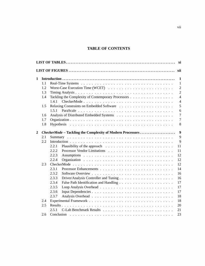
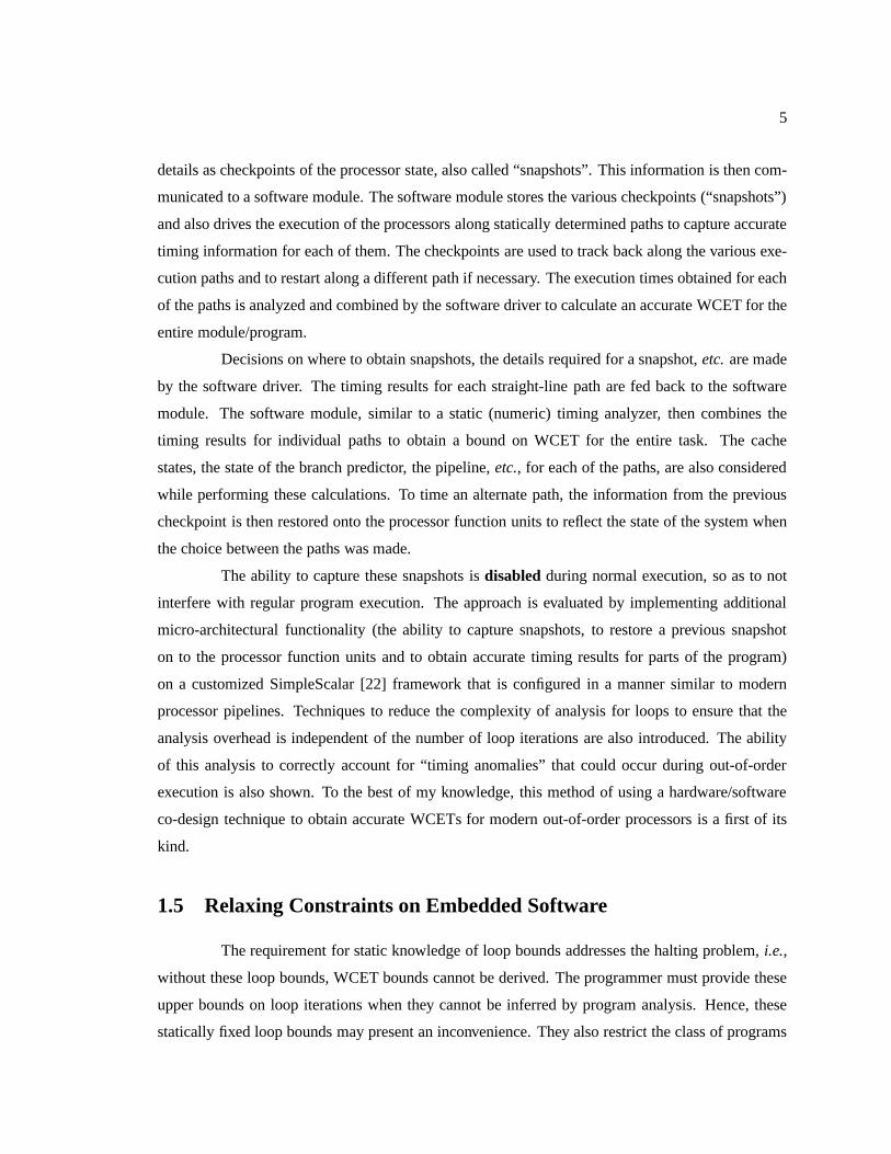
Figure 1.1 Static and dynamic analysis compared to actual execution time . . . . . . . . . . . . . . . . . 3

Figure 2.1 CheckerMode in Action . . . . . . . . . . . . . . . . . . . . . . .. . . . . . . . . . . . . . . . . . . . . . . . . . . . . 14

Figure 2.2 CheckerMode Design. . . . . . . . . . . . . . . . . . . . . . . . .. . . . . . . . . . . . . . . . . . . . . . . . . . . . . . 15

Figure 2.3 Control Flow Graph of Toy Benchmark and Measured Cycles . . . . . . . . . . . . . . . . . . 19

Figure 2.4 Measured Cycles (Aggregate Technique) for Synthetic Benchmark . . . . . . . . . . . . . . 20

Figure 2.5 Timing Results for the ADPCM Benchmark . . . . . . . . .. . . . . . . . . . . . . . . . . . . . . . . . . 21

Figure 2.6 Measured execution cycles for C-Lab Benchmarks .. . . . . . . . . . . . . . . . . . . . . . . . . . . 22

Figure 3.1 Model used for description and capture of Snapshots . . . . . . . . . . . . . . . . . . . . . . . . . . 27

Figure 3.2 Snapshot Captured using the DR Technique . . . . . . .. . . . . . . . . . . . . . . . . . . . . . . . . . . . 28

Figure 3.3 Definition of a Snapshot, based on the “Drain-Retire” mechanism . . . . . . . . . . . . . . . 29

Figure 3.4 Mechanism to Capture/Handle Structural Hazards. . . . . . . . . . . . . . . . . . . . . . . . . . . . . 30

Figure 3.5 Snapshot Merge Algorithm (DRM) . . . . . . . . . . . . . . .. . . . . . . . . . . . . . . . . . . . . . . . . . . 34

Figure 3.6 Merging using the DRM Algorithm . . . . . . . . . . . . . . .. . . . . . . . . . . . . . . . . . . . . . . . . . . 35

Figure 3.7 Incorrect Merge . . . . . . . . . . . . . . . . . . . . . . . . . . . .. . . . . . . . . . . . . . . . . . . . . . . . . . . . . . . . 36

Figure 3.8 Merging Reservation Stations . . . . . . . . . . . . . . . .. . . . . . . . . . . . . . . . . . . . . . . . . . . . . . . 37

Figure 3.9 Merge for Multiple Snapshots . . . . . . . . . . . . . . . . .. . . . . . . . . . . . . . . . . . . . . . . . . . . . . . 37

Figure 3.10 Anomaly Effects on Merge . . . . . . . . . . . . . . . . . . . .. . . . . . . . . . . . . . . . . . . . . . . . . . . . . . 38

Figure 3.11 Case 1 (a) (i)t′k is greater thantR{i} . . . . . . . . . . . . . . . . . . . . . . . . . . . . . . . . . . . . . . . . . . . 40

Figure 3.12 Case 1 (a) (ii)t′k is less thantR{i} . . . . . . . . . . . . . . . . . . . . . . . . . . . . . . . . . . . . . . . . . . . . . 40

Figure 3.13 Case 2 (a) (i)t′k is less thantR{i} . . . . . . . . . . . . . . . . . . . . . . . . . . . . . . . . . . . . . . . . . . . . . . 41

Figure 3.14 Case 2 (a) (ii)t′k is greater thantR{i} . . . . . . . . . . . . . . . . . . . . . . . . . . . . . . . . . . . . . . . . . . 42

xiii

Figure 3.15 Case 3 (a) neithert′k nor tR{i} change . . . . . . . . . . . . . . . . . . . . . . . . . . . . . . . . . . . . . . . . . 42

Figure 4.1 Counter example against use of only fixed point timing . . . . . . . . . . . . . . . . . . . . . . . . 50

Figure 4.2 Execution of counter example through the pipeline . . . . . . . . . . . . . . . . . . . . . . . . . . . . 50

Figure 4.3 A Second Fixed Point . . . . . . . . . . . . . . . . . . . . . . . . .. . . . . . . . . . . . . . . . . . . . . . . . . . . . . 53

Figure 4.4 Alternative Execution Scenario for counter example . . . . . . . . . . . . . . . . . . . . . . . . . . . 54

Figure 4.5 Synthetic Benchmark for Analyzing Stable state of Reservation Stations . . . . . . . . . 55

Figure 4.6 CFG . . . . . . . . . . . . . . . . . . . . . . . . . . . . . . . . . . . . . . .. . . . . . . . . . . . . . . . . . . . . . . . . . . . . . . 56

Figure 4.7 Measured execution cycles for loop path compositions (SRTbubblesortfunction) 57

Figure 4.8 Complete execution cycles for C-Lab Benchmarks –including loop WCECs . . . . . 61

Figure 4.9 δ’s for two and three level compositions for nine loops in ADPCM benchmark . . . 62

Figure 5.1 Static Timing Analysis Framework. . . . . . . . . . . . .. . . . . . . . . . . . . . . . . . . . . . . . . . . . . . 69

Figure 5.2 Numeric Loop Analysis Algorithm . . . . . . . . . . . . . .. . . . . . . . . . . . . . . . . . . . . . . . . . . . 70

Figure 5.3 Use of Parametric Timing Analysis . . . . . . . . . . . . .. . . . . . . . . . . . . . . . . . . . . . . . . . . . . 71

Figure 5.4 Parametric Loop Analysis Algorithm . . . . . . . . . . .. . . . . . . . . . . . . . . . . . . . . . . . . . . . . . 71

Figure 5.5 Syntactic and Semantic specifications for constraints on analyzable loops. . . . . . . . 73

Figure 5.6 Example of an outer loop with multiple paths . . . . .. . . . . . . . . . . . . . . . . . . . . . . . . . . . 74

Figure 5.7 WCET Bounds as a Function of the Number of Iterations . . . . . . . . . . . . . . . . . . . . . . 76

Figure 5.8 Flow of Parametric Timing Analysis . . . . . . . . . . . .. . . . . . . . . . . . . . . . . . . . . . . . . . . . . 77

Figure 5.9 Example of using Parametric Timing Predictions .. . . . . . . . . . . . . . . . . . . . . . . . . . . . . 78

Figure 5.10 Experimental Framework . . . . . . . . . . . . . . . . . . . .. . . . . . . . . . . . . . . . . . . . . . . . . . . . . . . 81

Figure 5.11 Energy consumption for PCG Wattch Model – Dynamic Energy consumption . . . . 87

Figure 5.12 PCGL-W – Leakage Consumption from the Wattch Model . . . . . . . . . . . . . . . . . . . . . 88

Figure 5.13 PCGL – Leakage Consumption from the Wattch Model. . . . . . . . . . . . . . . . . . . . . . . . 89

Figure 5.14 Energy Consumption Trends for increasing WCET Factors for ParaScale-G . . . . . . 91

xiv

Figure 5.15 Comparison of Dynamic Energy Consumption for ParaScale-G and Lookahead . . 93

Figure 6.1 Edges and Nodes in the Timing graph . . . . . . . . . . . . .. . . . . . . . . . . . . . . . . . . . . . . . . . . 104

Figure 6.2 Synchronization constructs . . . . . . . . . . . . . . . . .. . . . . . . . . . . . . . . . . . . . . . . . . . . . . . . . . 105

Figure 6.3 Deadlocks in Timing Graphs . . . . . . . . . . . . . . . . . . .. . . . . . . . . . . . . . . . . . . . . . . . . . . . . 105

Figure 6.4 Sample code to illustrate creation of the Timing Graph . . . . . . . . . . . . . . . . . . . . . . . . . 106

Figure 6.5 Timing graph created by application of various information gathering techniques . 108

Figure 6.6 Two Point-of-View Simplifications . . . . . . . . . . . .. . . . . . . . . . . . . . . . . . . . . . . . . . . . . . . 111

Figure 6.7 Remove direct red edges . . . . . . . . . . . . . . . . . . . . . .. . . . . . . . . . . . . . . . . . . . . . . . . . . . . . 112

Figure 6.8 Move outgoing red edges to successor . . . . . . . . . . .. . . . . . . . . . . . . . . . . . . . . . . . . . . . . 113

Figure 6.9 Move incoming red edges to predecessor . . . . . . . . .. . . . . . . . . . . . . . . . . . . . . . . . . . . . 114

Figure 6.10 Outcome of graph transformations . . . . . . . . . . . .. . . . . . . . . . . . . . . . . . . . . . . . . . . . . . . 115

Figure 6.11 Multiple producer-consumers . . . . . . . . . . . . . . .. . . . . . . . . . . . . . . . . . . . . . . . . . . . . . . . 115

Figure 6.12 Converting Blue edges to Red – creating futures .. . . . . . . . . . . . . . . . . . . . . . . . . . . . . . 116

Figure 6.13 Options for the Future . . . . . . . . . . . . . . . . . . . . . .. . . . . . . . . . . . . . . . . . . . . . . . . . . . . . . . 117

1

Chapter 1

Introduction

Every year,billions of microprocessors are sold for use in embedded systems [120]. This

is in sharp contrast to a few hundred million desktop processors that are sold in the same time-

frame. From automobiles to medical equipment, thermostatsto space shuttles, embedded systems

are all around us. Moreover, the use of embedded systems is increasing, if anything, with the advent

of “Cyber-Physical Systems” (CPS), which can be described as “integrations of computation with

physical processes.” Hence, cyber-physical systems affect and are affected bythe physical world

and the environment that they operate in. The modern automobile and evensmart homesfall into

this category. They are typically comprised of networks andcombinations of smaller embedded

systems that perform specific tasks.

1.1 Real-Time Systems

The software and hardware used for embedded and cyber-physical systems, in general,

must be validated, which traditionally amounts to checkingthe correctness of the input/output rela-

tionship. Many such systems also impose timing constraintson the execution times of constituent

tasks. Violations of these constraints (often referred to as “deadlines”) could lead to fallouts that are

dangerous to users, the environment or both. Such systems are commonly referred to as “real-time

systems”, and they impose temporal constraints on computational tasks to ensure that results are

available on time. Often, approximate results supplied in time are preferred to more precise results

that may become available late,i.e., after the passage of deadlines.

Consider the case of the Anti-lock Braking System (ABS) [135] found in most modern

automobiles. It consists of a rotating road wheel that prevents a locked wheel or a “skid” under

2

heavy braking. The driver is able to maintain control by the ABS as it allows the wheel to roll for-

ward. In fact, recent versions not only perform the ABS functionality but also Electronic Brakeforce

Distribution (EBD), Traction Control System (TCS), Electronic Stability Control (ESC),etc.. The

ABS system is a classic example of areal-time, embedded systemthat we encounter in everyday

life. If a driver must hit the brakes of a car in an emergency, then the ABS must kick in and function

correctly in themilliseconds (perhaps even microseconds) time-frame. It is absolutely useless if it

functions correctly, sayten secondsafter the brakes have been pressed – in fact, a failure to operate

in the short, required duration might result in a loss of human life and/or damage to property. Nu-

clear reactor controls, electronic engines, modern avionics – all of these applications fall under the

purview of real-time systems and have stringent design criteria. They require advance knowledge

of the properties of and guarantees on the behavior of the system, the most critical of which is that

no task in the system misses its deadline.

1.2 Worst-Case Execution Time (WCET)

Schedulability analysis [77] is used to guarantee that a given system of real-time tasks

will be able to meet its deadlines on a particular hardware system. One critical piece of informa-

tion required for such analysis is the “worst-case execution time” (WCET) of each task, which is

defined as

“the guaranteedworst-case time taken by the task to execute on aspecifichardwareplatform.”

The process of determining the WCET of a task is known as “timing analysis” and is often charac-

terized as being either(a) statictiming analysis or(b) dynamictiming analysis.

1.3 Timing Analysis

Timing analysis has become an increasingly popular research topic. This can be attributed

in part to the problem of increasing architectural complexity, which makes applications less pre-

dictable in terms of their timing behavior, but it may also bedue to the abundance of embedded

systems that we have recently seen. Often, application areas of embedded systems impose stringent

timing constraints, and system developers are becoming aware of a need for verified bounds on exe-

cution times. Thetighter these bounds relative to the true worst-case times, the greater the value of

3

the analysis. Of course, even a tight bound has to be asafe boundin that it must not underestimate

the true WCET; it may only match or exceed it.

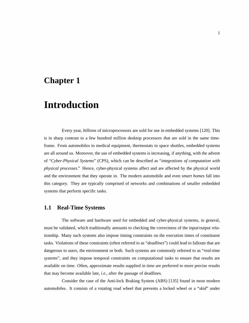
Static timing analysis[14, 15, 26, 27, 34, 36, 49, 52, 53, 59, 73, 74, 82, 84, 89, 94, 97, 103,

119,126,133] techniques suffer from the drawback that theyare either overly pessimistic or impose

severe constraints on the types of code that may be analyzed (e.g., known upper bounds on loops,

absence of function pointers and no heap allocation). If such an analysis is pessimistic, as shown

in Figure 1.1, then system resources may be wasted. Bounds onexecution times require constraints

to be imposed on the tasks (timed code), the most striking of which is the requirement to statically

bound the number of iterations of loops within the task. Complex architectural features, such as

out-of-order (OOO) processing [96] and branch prediction [113], are often beyond the reach of

static analyses, mainly due to the fact that they introduce non-determinism into the task code. These

issues cannot be resolved at compile time, thus forcing real-time system designers to completely

avoid the use of such processors.

Dynamic timing analysismethods [14,15,19,119,125,127], on the other hand, are either

trace-driven, experimental or stochastic in nature. They are unable to guarantee the safety of WCET

values obtained [126]. Architectural complexities, difficulties in determining worst-case input sets

and the exponential complexity of performing exhaustive testing over all possible inputs are also

reasons why dynamic timing analysis methods are unsafe and,hence, infeasible in general. The

threat of dynamic methods is that the execution time of tasksmight actually beunderestimated

(as shown in Figure 1.1), which can result in serious errors during system operation, implying

potentially dangerous fallouts.

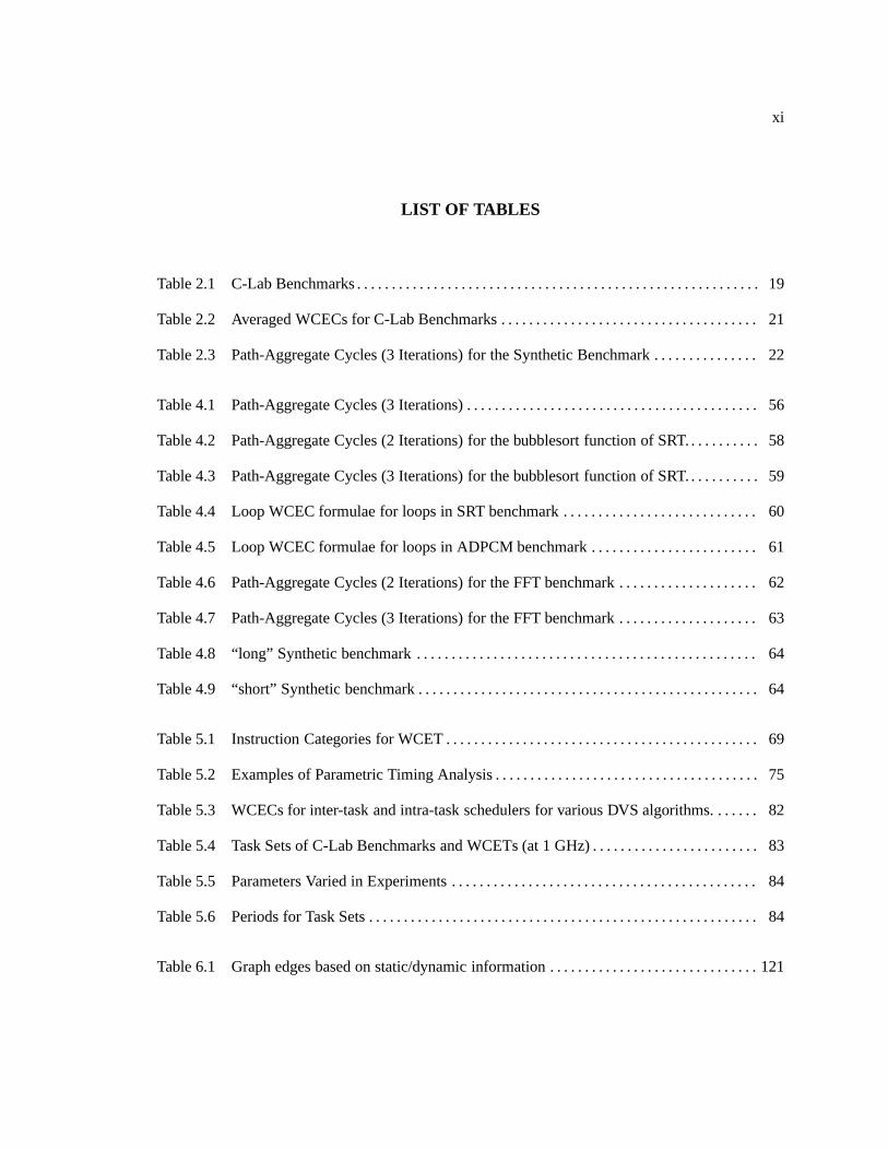
actualdynamic

static

static

dynamicactual

longest

shortest

dyn. measurements

Figure 1.1: Static and dynamic analysiscompared to actual execution time

The objective of any timing analysis technique

is to approximate the worst-caseactualexecution time of

a task, i.e., the longest possible execution time consid-

ering all inputs and hardware complexities, deterministic

or not. The more closely this value is approximated, the

easier it is to design the system in an accurate, safe and

efficient manner in terms of resource usage. Determina-

tion of the WCET bounds of a task is a non-trivial process

due to a variety of reasons, broadly classified into:

1. hardware complexities: non-determinism of modern architectural features, process varia-

tions during the manufacturing of microprocessors,etc.; and

4

2. software complexities: non-determinism of inputs, complexity of task code,etc.

This work addresses these shortcomings on both fronts –hardwareas well assoftware.

Section 1.4 briefly discusses novel techniques to tackle hardware and architectural complexity while

Section 1.5 introduces techniques to relax constraints imposed on task code. Section 1.6 introduces

techniques aimed at analyzing complex embedded software – containing multiple threads that could

potentially bedistributed in nature. It also demonstrates applications where timing analysis tech-

niques could be utilized to analyze complex systems. All of these techniques utilize the interactions

and passing of information between hardware and software toincrease the accuracy of the analysis.

The main idea is that a single source of information (such as only static or only dynamic analysis

methods) is not sufficient for analyzing modern embedded systems that are inherently complex.

Thus, novel methods that utilize information from multiple sources is required for a more

complete analysis.

1.4 Tackling the Complexity of Contemporary Processors

A serious handicap in performing static timing analysis is the complexity of modern pro-

cessors and their functional units. Various features that decreaseaverageexecution times for tasks

are often detrimental for worst-case timing analysis. Out of order (OOO) processing [96] and branch

prediction [113] are two important features in modern processors that introduce non-determinism

to task execution, which cannot be resolved at compile time [12,23,35]. Other issues that increases

the complexity of the analysis are the presence ofstatically indeterminate loopsin task code and

timing anomalies[13,79,81,109]. Hence, designers of real-time systems areoften forced to use less

complicated, older and inherently less powerful processors. While this guarantees determinism, it

neglects performance. The following section (1.4.1) introduces the concept of “hybrid” timing anal-

ysis that utilizes interactions between a software timing analyzer and run-time information from the

actual microprocessor to obtain tight WCET estimates on contemporary processors.

1.4.1 CheckerMode

The task of obtaining accurate timing analysis results for modern, out-of-order proces-

sors is achieved by the use of theCheckerModeinfrastructure. Minor enhancements to the micro-

architecture of future processors are proposed. These willaid in the processes of obtaining tight

WCET bounds. A “checker mode” is added to processors that will, on demand, capture varying

5

details as checkpoints of the processor state, also called “snapshots”. This information is then com-

municated to a software module. The software module stores the various checkpoints (“snapshots”)

and also drives the execution of the processors along statically determined paths to capture accurate

timing information for each of them. The checkpoints are used to track back along the various exe-

cution paths and to restart along a different path if necessary. The execution times obtained for each

of the paths is analyzed and combined by the software driver to calculate an accurate WCET for the

entire module/program.

Decisions on where to obtain snapshots, the details required for a snapshot,etc.are made

by the software driver. The timing results for each straight-line path are fed back to the software

module. The software module, similar to a static (numeric) timing analyzer, then combines the

timing results for individual paths to obtain a bound on WCETfor the entire task. The cache

states, the state of the branch predictor, the pipeline,etc., for each of the paths, are also considered

while performing these calculations. To time an alternate path, the information from the previous

checkpoint is then restored onto the processor function units to reflect the state of the system when

the choice between the paths was made.

The ability to capture these snapshots isdisabled during normal execution, so as to not

interfere with regular program execution. The approach is evaluated by implementing additional

micro-architectural functionality (the ability to capture snapshots, to restore a previous snapshot

on to the processor function units and to obtain accurate timing results for parts of the program)

on a customized SimpleScalar [22] framework that is configured in a manner similar to modern

processor pipelines. Techniques to reduce the complexity of analysis for loops to ensure that the

analysis overhead is independent of the number of loop iterations are also introduced. The ability

of this analysis to correctly account for “timing anomalies” that could occur during out-of-order

execution is also shown. To the best of my knowledge, this method of using a hardware/software

co-design technique to obtain accurate WCETs for modern out-of-order processors is a first of its

kind.

1.5 Relaxing Constraints on Embedded Software

The requirement for static knowledge of loop bounds addresses the halting problem,i.e.,

without these loop bounds, WCET bounds cannot be derived. The programmer must provide these

upper bounds on loop iterations when they cannot be inferredby program analysis. Hence, these

statically fixed loop bounds may present an inconvenience. They also restrict the class of programs

6

that can be used in real-time systems. This type of timing analysis is referred to asnumerictiming

analysis [49,52,53,94,132,133] since it results in a single numeric value for WCET given the upper

bounds on loop iterations. The constraint on the known maximum number of loop iterations is

removed byparametrictiming analysis (PTA) [124], which is used in theParaScaleinfrastructure,

introduced in Section 1.5.1.

1.5.1 ParaScale

Parametric timing analysis permits variable-length loops. Loops may be bounded byn

iterations as long asn is known prior to loop entry during execution. Such a relaxation widens the

scope of analyzable programs considerably and facilitatescode reuse for embedded/real-time ap-

plications. This work describes (a) the application of static timing analysis techniques to dynamic

scheduling problems and (b) assesses the benefits of PTA for dynamic voltage scaling (DVS). This

work contributes a novel technique that allows PTA to interact with a dynamic scheduler while dis-

covering actual loop bounds during execution prior to loop entry. At loop entry, a tighter bound on

the WCET can be calculated on-the-fly, which may then triggerscheduling decisions synchronous

with the execution of the task.

The benefits of using PTA to analyze code sections is evaluated by measuring power

savings in the system. Power savings are typically achievedby means of dynamic voltage scaling

(DVS) or dynamic frequency scaling (DFS) techniques. TheParaScaleinfrastructure utilizes a

combination of inter, and intra-task DVS techniques to achieve power savings. ParaScale uses the

results of PTA by using parametric formulae, evaluated at run-time, to make dynamic decisions on

the amount of execution completed, amount of slack left, andfrequency/voltage scaling to reduce

power consumption. An intra-task scheduler is used for thispurpose. Hence, ParaScale provides

the ability to evaluate the benefits of PTA on a system.

The ParaScale approach utilizes online intra-task DVS to exploit parametric execution

times resulting in much lower power consumptions,i.e., even without any scheduler-assisted DVS

schemes. Hence, even in the absence of dynamic priority scheduling, significant power savings may

be achieved,e.g., in the case of cyclic executives or fixed-priority policies, such as rate-monotone

schedulers [76]. Overall, parametric timing analysis expands the class of applications for real-time

systems to include programs with dynamic loop bounds that are loop invariant while retaining tight

WCET bounds and uncovering additional slack in the schedule.

7

1.6 Analysis of Distributed Embedded Systems

Cyber-physical systems operate on a variety of embedded hardware ranging from 8-bit

microcontrollers to sophisticated multicores. Knowledgeof the temporal behavior of an application

is hidden inside the application logic, where it is extremely difficult to extract, analyze and model

for any given hardware. While static and dynamic timing analyses are used to obtain the worst-case

execution times (WCETs) for real-time applications, they may not be able to provide a complete pic-

ture of a program. This is particularly true in the case of larger, more complex programs. Programs

that contain function pointers are typically out of reach ofstatic analyzers. Dynamic analyzers are

unable to gauge the true nature of the program and have shown to be unsafe –i.e., they may under-

estimate the WCET of the program, which could lead to dangerous effects. If the application uses

concurrency constructs, such as signals, locks or mutexes,then neither of these techniques can fully

analyze the application.

The work presented here studies the use of combinations of a variety of techniques to

form the complete picture of the structure and execution characteristics of a distributed embedded

application. The results obtained are collected to createtiming graphs, the topology of which can

be studied to extractmeaningabout the application. This information can then be used to

• provide information to the designers of the system to be usedto identify problematic areas in

the application and to

• tailor the amount of parallelism in the system so that the same application can execute on

small embedded microcontrollers as well as large, modern multicore processors.

1.7 Organization

The remainder of this dissertation is loosely split into three parts:

1. CheckerMode: Chapter 2 describes the overall design for the CheckerModeframework to

tackle the complexities of modern architectures (first published at RTAS 2008 [86]). Chapter 3

contains the analysis of how the CheckerMode framework is able to handle timing anomalies

that occur during OOO execution (acceptedfor publication at RTSS 2008 [87]). Chapter 4

explains the analysis techniques that are able to accurately analyze statically indeterminate

loops without enumerating all iterations.

8

2. ParaScale: Chapter 5 describes the ParaScale infrastructure used to relax constraints on em-

bedded software, the results from which are used to attain power savings (published in RTSS

2005 [89] and the TECS journal [88]).

3. Distributed Embedded Systems: Chapter 6 discusses techniques used to analyze distributed

embedded systems (published in ECRTS 2008 [85]).

Chapter 7 presents the related work. Chapter 8 presents ideas for future work while Chap-

ter 9 presents the conclusion.

1.8 Hypothesis

Modern embedded systems with timing constraints are too complex to be analyzed by

any single technique alone due to the non-determinism introduced by hardware features as well as

complexities in software. Hence, the hypothesis of this dissertation is that

by employing a combination of multiple analysis techniques, multiple sources of infor-mation and constant interactions between hardware and software it becomes feasible togauge the worst-case behavior of modern embedded systems that utilize contemporaryprocessors and complex software constructs.

The analysis presented is constrained to

1. analyzingout-of-order processor pipelines, correct handling oftiming anomaliesand loops

around them; to

2. providing power savings by removing constraints that enforce statically determinate loop

bounds; and to

3. reason aboutdistributed real-time embedded systemsthat have basiccommunication and syn-

chronization constructs.

9

Chapter 2

CheckerMode – Tackling the Complexity

of Modern Processors

2.1 Summary

A limiting factor for designing real-time systems is the class of processors that can be

used. Typically, modern, complex processor pipelines cannot be used in real-time systems design.

Contemporary processors with their advanced architectural features, such as out-of-order execu-

tion, branch prediction, speculation, prefetching,etc., cannot be statically analyzed to obtaintight

WCET bounds for tasks. This is caused by the non-determinismof these features, which surfaces

in full only at runtime. This chapter introduces a new paradigm to perform timing analysis of tasks

for real-time systems running on modern processor architectures. Minor enhancements to the pro-

cessor architecture are proposed to enable this process. These features, on interaction with software

modules, are able to obtain tight, accurate timing analysisresults for modern processors.

2.2 Introduction

Static timing analysis [15, 27, 34, 59, 84, 89, 94, 103, 119] provides bounds on the WCET

of tasks. Thetighter that these bounds are relative to the actual worst-case times, the greater the

value of the analysis. Of course, even tight bounds must besafein that the true WCET mustnever

be underestimated; the WCET bound may at most match or otherwise overestimate the true WCET.

A serious handicap in performing static timing analysis is the complexity of modern pro-

cessors and their functional units. Various features that decreaseaverageexecution times for tasks

10

are often detrimental for worst-case timing analysis. Out of order (OOO) processing [96] and branch

prediction [113] are two important features in modern processors that introduce non-determinism to

task execution, which cannot be resolved at compile time [12,23,35]. Hence, designers of real-time

systems are often forced to use less complicated, older and inherently less powerful processors. In

this chapter, techniques to bridge this gap by means of theCheckerModeinfrastructure are pre-

sented. CheckerMode combines the best features of both, static and dynamic analysis, to create a

novel hybrid mechanism for WCET analysis.

Minor enhancements to the micro-architecture of future processors are presented that will

aid in the process of obtaining accurate WCET bounds. A “checker mode” is added to processors

that will, on demand, capture varying levels of informationas “snapshots” of the processor state.

This information is communicated to a software module that stores the various snapshots and also

drives the execution of instructions in the processor alongstatically determined paths. Accurate

timing information for each path is then captured. These snapshots are also used to backtrack to

an earlier state and then restart along a different path. Execution times obtained for each path are

analyzed and then combined by the software driver to calculate an accurate WCET for the entire

program/function.

Decisions on where to obtain snapshots, the level of detail required for each snapshot,etc.

are made by the software controller (“driver”). Timing results for each straight-line path are then

fed back to the software module. The software module (similar to a static/numeric timing analyzer),

then combines the timing results for individual paths to obtain a bound on WCET for the entire task.

The cache states, the state of the branch predictor, the pipeline, etc., for each of the paths, are also

considered while performing these calculations. To time analternate path, the information from

the previous snapshot is restored onto the processor function units to reflect the state of the system

when the choice between the paths was made.

The ability to capture these snapshots is disabled during normal execution, so as to not

interfere with regular program execution. The approach is evaluated by implementing additional

micro-architectural functionality (the ability to capture snapshots, to restore a previous snapshot

on to the processor function units and the ability to obtain accurate timing results for parts of the

program) on a customized SimpleScalar [22] framework that is configured in a manner similar to

modern processor pipelines.

To the best of my knowledge, this method of using a hardware/software co-design tech-

nique to obtain accurate WCETs for modern out-of-order processors is a first of its kind.

11

2.2.1 Plausibility of the approach

The proposed hardware enhancements are realistic. The support for speculative execution

due to dynamic branch prediction, precise exception handling and precise hardware monitoring,

and even most of the internal buffers required by the CheckerMode design already exist in modern

high-end embedded processors. For example, the ARM-11 features out-of-order execution, dy-

namic branch prediction, and precise traps, which requiresshadow buffers (for registers, branch

history tablesetc.) [28] in order to recover to a prior execution state. In addition to these fea-

tures, the Intel x86 architecture supports Precise Event Based Sampling (PEBS) with user access

to selected shadow buffers [114]. Future processor extensions also make heavy use of checkpoint

buffers [29, 30, 66]. CheckerMode’s design will make such buffers uniformly available to the user.

Enhancements to the ALU and branch logic to handle the new semantics for NaN (Not-A-Number)

operands are required by CheckerMode (see Section 2.3), which are minor modifications compared

to the space and complexity of the already existing shadow buffers. In fact, most processors already

implement a NaN representation for floating point values (and an equivalent bottom value for inte-

gers), which is generated when undefined arithmetic (e.g., divide-by-zero) is performed and results

in an exception (trap). The sole modification suggested would be to gate the exception,i.e., suppress

it in CheckerMode, and proceed with arithmetic operations in the presence of NaN values.

2.2.2 Processor Vendor Limitations

One other shortcoming of static timing analysis approachesdeveloped so far is given by

their targeting of a generic processor type based on vendor-supplied design details. In such an

approach, each new processor design requires that the timing model be manually adapted while

the CheckerMode technique automatically adapts with changing processor details. Furthermore,

such timing models are only as good as the information provided by the vendor, which may not

reveal all details of the design. For example, Intel’s CPU stepping index indicates subtle processor

modifications within the same CPU family but does not reveal all details.

In fact, fabrication variability due to smaller feature sizes in the smallest production pro-

cesses used to date already result in timing variability between two processors originating from the

same batch [16–18, 61]. Taken to the extreme, access latencies within a cache may actuallydiffer

from one line to another or equivalent functional units may have different micro-timing characteris-

tics. Hence, generic timing analysis of a processor line becomes meaningless in such a setting. The

CheckerMode infrastructure avoids this detailed level of processor modeling and allows vendors to

12

protect their IP while providing a method to obtain highly accurate timing. Since CheckerMode

observes the execution time on an actual processor, such variability is captured.

CheckerMode widens the scope of processors that may be used in a real-time system.

Contemporary processors with state-of-the-art functionality and performance may subsequently be

used in real-time systems. This also changes the landscape for timing analysis in that more accurate

results can be obtained on modern pipelines without risk of losing functionality. In a world of

increasingly specialized components, the idea that some processors could be designed specifically

for use in real-time and embedded systems has already caughton,e.g., with designs that customize

generic core, such as the ARM-7/9/11 licensed by Qualcomm and many others. This is especially

true in the design and testing phases for the real-time systems being created. These processors would

not behave any differently during normal execution but would only have the additional characteristic

that more information can be gathered from them during the analysis phase. Hence, there is an

assurance that the additional features will not further complicate the analysis.

2.2.3 Assumptions

CheckerMode, in its current state only addresses the unpredictable nature of out-of-order

instruction execution in contemporary high-end embedded processor pipelines. Other complexities,

such as memory hierarchies, including caches, and dynamic branch prediction are beyond the scope

of this initial work and will be addressed in the future. Tasks are analyzed inisolation. Preemptions

and cache-related preemption delays, handled by orthogonal work [105], could be incorporated in

the future and should not require any changes to the CheckerMode approach since their analysis

occurs at a higher level.

2.2.4 Organization

This chapter is organized as follows. Section 2.3 introduces the CheckerMode infras-

tructure. Section 2.4 explains the experimental setup. Section 2.5 enumerates the results from the

experiments while Section 2.6 summarizes the high-level contributions.

2.3 CheckerMode

The CheckerModeinfrastructure, detailed in this section, provides the means to obtain

accurate WCET values for modern processor pipelines. It encompasses enhancements/additions to

13

the microarchitecture while closely interacting with software to obtain WCET bounds. The idea

is to design embedded processors, that in addition to executing software normally (in a so-called

deployment mode), are capable of executing in a novelCheckerModethat supports timing analysis.

CheckerMode provides cycle-accurate bounds on the WCET by assessing alternate exe-

cution paths in a program. In deployment mode, a processor executes along just one path following

a conditional branch; which path is executed may depend on the input data. In CheckerMode, a

processor no longer proceeds with conventional data-driven execution. Instead, it executes all alter-

nate paths, one at a time, following each conditional branchin order to find the path with the largest

execution time. Before the execution of each alternate path, the original execution context (includ-

ing caches, branch history tables etc.) is restored to correctly simulate the effect of alternations in

isolation from one another. These low-level WCET results are propagated inter-procedurally in a

bottom-up fashion (over the combined control-flow and call graphs) until the WCET for an entire

task has been computed.

Consider a task that consists of a number of feasible execution paths. The execution times

for these paths are obtained by actual execution in CheckerMode through the processor pipeline.

The execution time for each path is then captured and stored.When conditional execution arises, all

alternate paths are timed separately on the pipeline. The timing information as well as the “state”

of the processor (determined by the cache state, branch predictor state, register state,etc.) are

combined when alternate paths join. The combination is performed such that the state that results

from the combination must not underestimate the execution time of the alternate paths or even the

future execution of the task. A set of timing schemes for individual paths as well as combinations

of paths, derived from this methodology, is discussed in theresults section.

Prior to the execution of alternate paths, a “snapshot” of the processor state is obtained and

stored. After the execution of one of the alternate paths, its state is recorded for later combination

with other paths. Then, the state of the processor is restored to the one that existed before the path

started executing. This is achieved by restoring the state (e.g., of each of the parts of the pipeline)

from the previously captured snapshot.

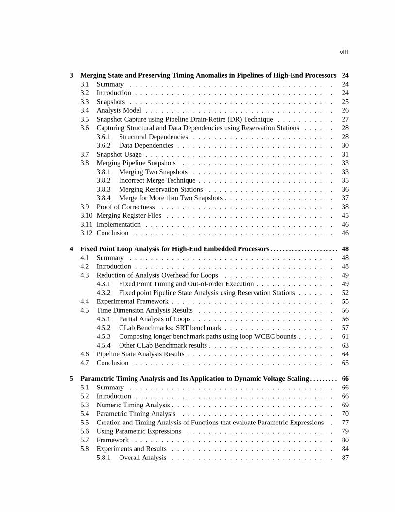
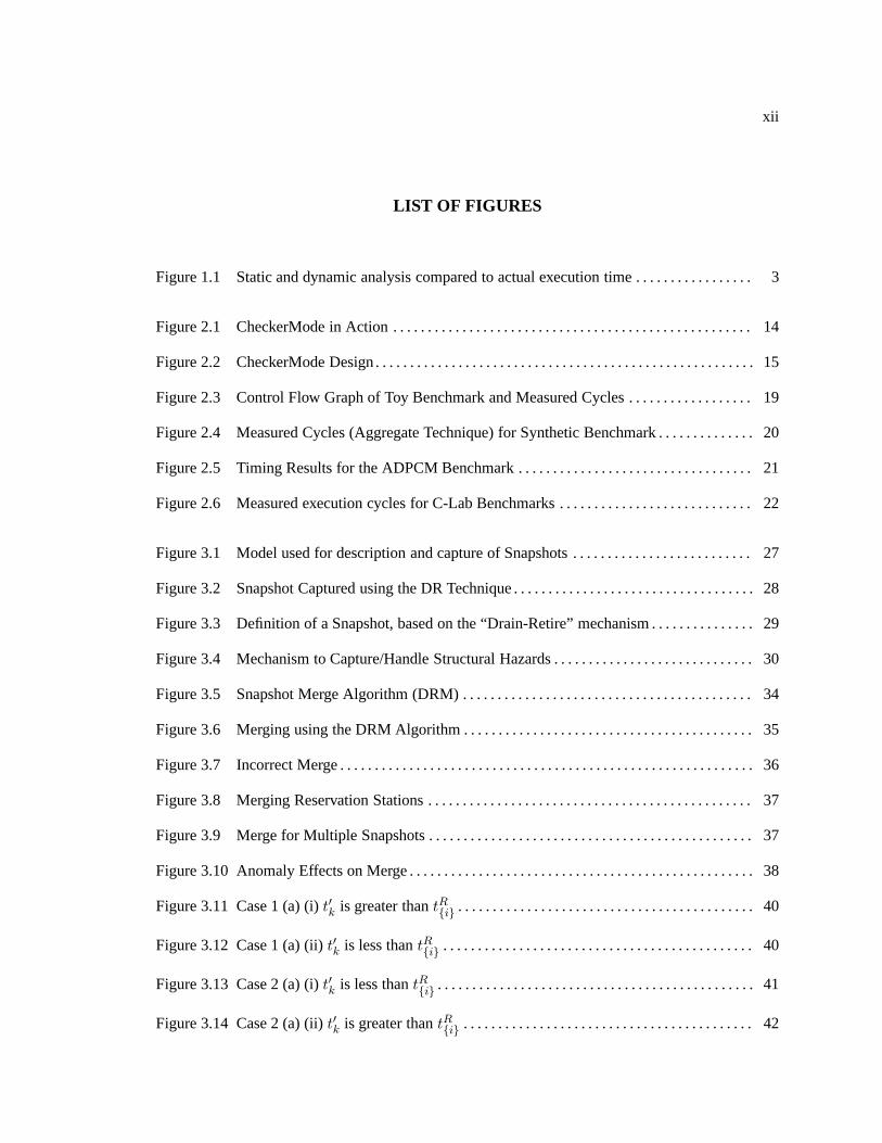
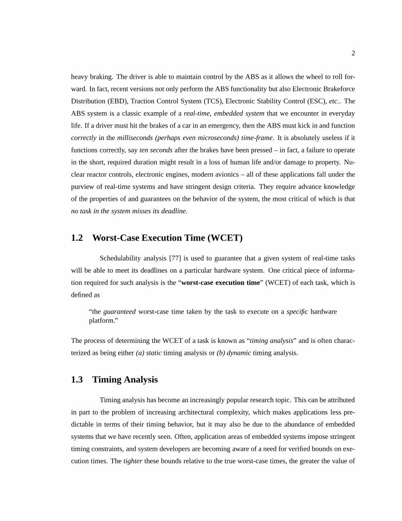
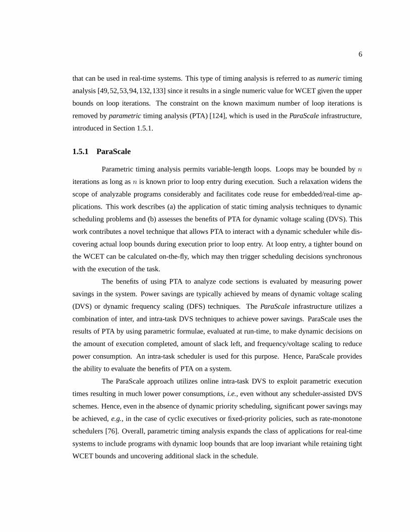
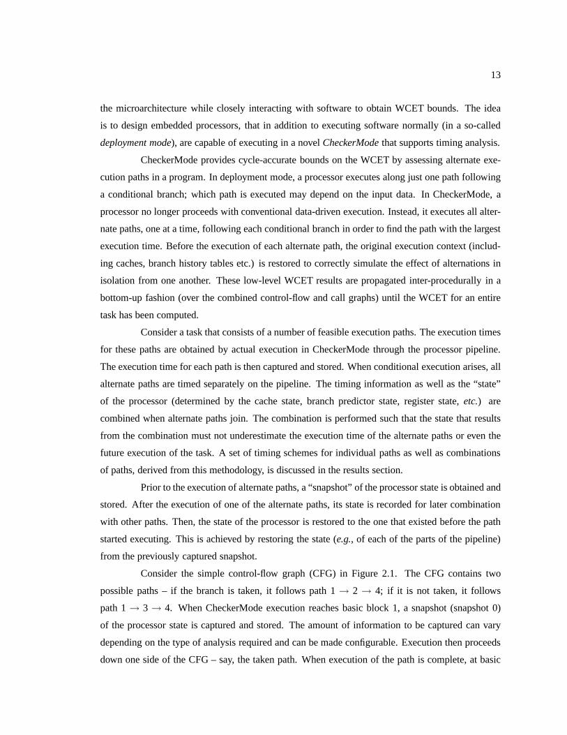
Consider the simple control-flow graph (CFG) in Figure 2.1. The CFG contains two

possible paths – if the branch is taken, it follows path 1→ 2 → 4; if it is not taken, it follows

path 1→ 3→ 4. When CheckerMode execution reaches basic block 1, a snapshot (snapshot 0)

of the processor state is captured and stored. The amount of information to be captured can vary

depending on the type of analysis required and can be made configurable. Execution then proceeds

down one side of the CFG – say, the taken path. When execution of the path is complete, at basic

14

block 4, another snapshot (snapshot 1) of the processor state is captured and stored. The time taken

to execute this path is also measured and sent to the timing analyzer. The program counter is then

reset to basic block 1 (the branch condition) to trace execution down the other side (not-taken) and

to subsequently capture the execution time for that path. Before execution proceeds along the not-

taken path, the state of the processor isrestoredto the previously saved snapshot (snapshot 0). This

isolates the effects of execution of one path from that of another. Once the processor state from

snapshot 0 is written back, execution from basic block 1 proceeds down the not-taken path (1→

3→ 4) before the processor state (snapshot 2) and execution time are captured once again. Only

then can the CheckerMode unit shift its focus to the code thatfollows basic block 4. For execution

to proceed from basic block 4, the processor must be set to a consistent state. At this point, it is

necessary to perform amergeof the snapshots from the two paths. The merge must be performed

such that the worst-case behavior of the subsequent code is preserved. Hence, we must merge the

state of all processor units captured in preceding snapshots. Once a merge has been performed, the

new state must be written back to the processor and executioncontinues from that point on.

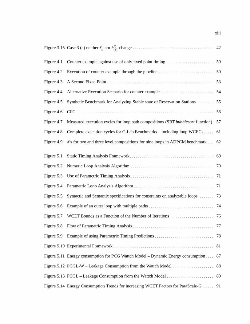
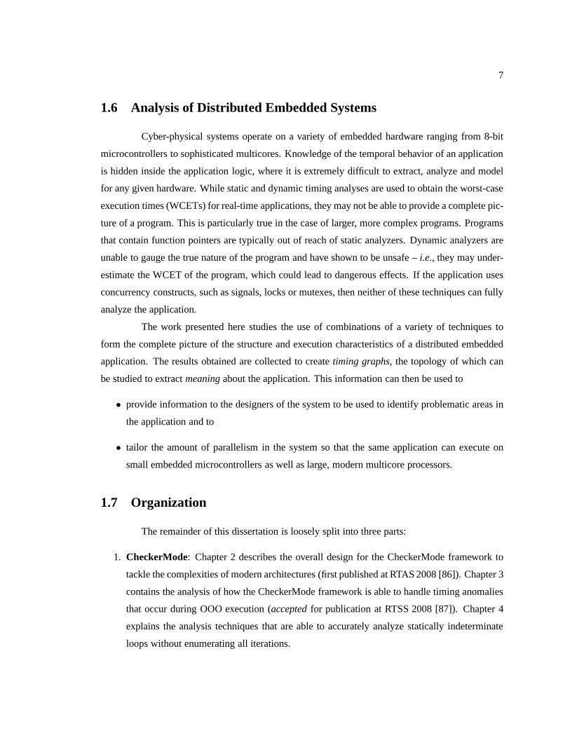
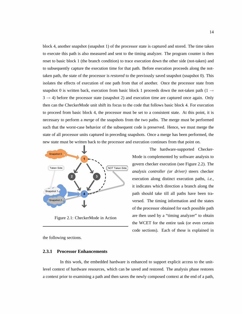
Figure 2.1: CheckerMode in Action

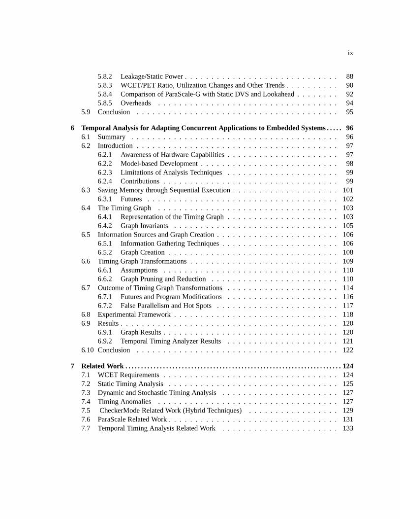
The hardware-supported Checker-

Mode is complemented by software analysis to

govern checker execution (see Figure 2.2). The

analysis controller (or driver)steers checker

execution along distinct execution paths,i.e.,

it indicates which direction a branch along the

path should take till all paths have been tra-

versed. The timing information and the states

of the processor obtained for each possible path

are then used by a “timing analyzer” to obtain

the WCET for the entire task (or even certain

code sections). Each of these is explained in

the following sections.

2.3.1 Processor Enhancements

In this work, the embedded hardware is enhanced to support explicit access to the unit-

level context of hardware resources, which can be saved and restored. The analysis phase restores

a context prior to examining a path and then saves the newly composed context at the end of a path,

15

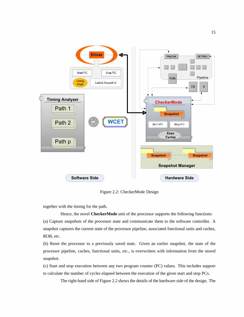
Figure 2.2: CheckerMode Design

together with the timing for the path.

Hence, the novelCheckerModeunit of the processor supports the following functions:

(a) Capturesnapshotsof the processor state and communicate them to the software controller. A

snapshot captures the current state of the processor pipeline, associated functional units and caches,

ROB, etc.

(b) Reset the processor to a previously saved state. Given anearlier snapshot, the state of the

processor pipeline, caches, functional units,etc., is overwritten with information from the stored

snapshot.

(c) Start and stop execution between any two program counter(PC) values. This includes support

to calculate the number of cycles elapsed between the execution of the given start and stop PCs.

The right-hand side of Figure 2.2 shows the details of the hardware side of the design. The

16

CheckerMode unit must be able to read and write to the variousfunctional units of the processor.

The CheckerMode unit is controlled by the driver (or controller) on the software side.

2.3.2 Software Overview

The left-hand side of Figure 2.2 illustrates the various components that make up the soft-

ware side of the design. It consists of the following components:

Timing Analyzer (TA): The TA breaks down the task code into a control-flow graph (CFG) and

then extracts path information from it. Using this information, the TA is able to determine the start

of alternate execution flows – points where snapshots must beobtained. It also provides the start

and stop PCs to the driver and obtains the WCET and processor state for that particular path from

the driver.

Snapshot Manager (SM):The SM maintains various snapshots that have been captured as well

as the PCs at which they were obtained. SM abstractions can beintegrated into the processor as

depicted in Fig. 2.2, or, alternately, into the driver within the software controller.

Driver: The driver controls the hardware side of the system. It instructs the hardware on when to

start and stop execution, when snapshots must be captured, and when the state of the processor must

be reset to a previous snapshot, as detailed below.

The input to the TA is the executable of a task. Assembly information is extracted (with

PCs) from an executable and then converted to internal representations as combined control-flow

and call graphs. The start and stop PCs provided by the TA encapsulate a single path. The TA, the

driver, and the SM interact to decide which snapshot corresponds to which path, which PC,etc., and

thereby control program execution.

The TA is responsible for obtaining the final WCET for the entire program as well as

various program segments (functions/scopes). It “combines” the information from various paths

(execution time, pipeline state,etc.) for this purpose. The driver, also part of the software system,

is described in more detail below.

2.3.3 Driver/Analysis Controller and Tuning

The driver is responsible for controlling processor operations. Besides directing the exe-

cution of the code on the pipeline, it relays instructions from the TA such as when to capture/restore

snapshots. The driver represents the interface between thehardware and software components of

the CheckerMode design. The driver contains information about the start and stop PCs that define

17

the start/end points of the path to be timed. It also stores the latest captured snapshot. The driver

maintains information about which instruction is a branch and where snapshots need to be captured.

It also relays information in the other direction – from the hardware to the timing analyzer –e.g.,

the path execution time.

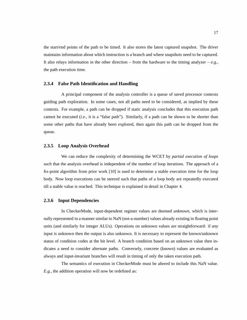
2.3.4 False Path Identification and Handling

A principal component of the analysis controller is a queue of saved processor contexts

guiding path exploration. In some cases, not all paths need to be considered, as implied by these

contexts. For example, a path can be dropped if static analysis concludes that this execution path

cannot be executed (i.e., it is a “false path”). Similarly, if a path can be shown to be shorter than

some other paths that have already been explored, then againthis path can be dropped from the

queue.

2.3.5 Loop Analysis Overhead

We can reduce the complexity of determining the WCET bypartial execution of loops

such that the analysis overhead is independent of the numberof loop iterations. The approach of a

fix-point algorithm from prior work [10] is used to determinea stable execution time for the loop

body. Now loop executions can be steered such that paths of a loop body are repeatedly executed

till a stable value is reached. This technique is explained in detail in Chapter 4.

2.3.6 Input Dependencies

In CheckerMode, input-dependent register values are deemed unknown, which is inter-

nally represented in a manner similar to NaN (not-a-number)values already existing in floating point

units (and similarly for integer ALUs). Operations on unknown values are straightforward: ifany

input is unknown then the output is also unknown. It is necessary to represent the known/unknown

status of condition codes at the bit level. A branch condition based on an unknown value then in-

dicates a need to consider alternate paths. Conversely, concrete (known) values are evaluated as

always and input-invariant branches will result in timing of only the taken execution path.

The semantics of execution in CheckerMode must be altered toinclude this NaN value.

E.g., the addition operation will now be redefined as:

18

rresult =

NaN if ra = NaN∨

rb = NaN

ra + rb otherwise

Hence, any operation with NaN as one of the operands will result in NaN (unless the

result is independent of that particular operand,e.g., multiplication with 0 will always result in

0). Similar enhancements are developed for other instructions that depend on input-dependent or

memory-loaded operands.

2.3.7 Analysis Overhead

The process of timing analysis now amounts to timing sequences of paths by saving and

restoring snapshots of processor state in a coordinated fashion. While this process can be lengthy,

it still remains independent of the input to the program, andin the worst-case, can be run overnight.

Since this is anoffline task to be performed during system design and validation, the cost is sec-

ondary and does not affect the dynamic, run-time behavior ofthe system. Sometimes such a full

verification of WCET bounds is generally only warranted after extensive code changes during de-

velopment and for each software deployment, including system upgrades. In practice though, safety

requirements of hard real-time systems demand that this level of verification be carried out for even

the smallest changes. During system development, it could be performed after larger changes from

time to time but must finally be performed fully at least once before the final deployment.

2.4 Experimental Framework

The key components of the CheckerMode design were implemented in the SimpleScalar

processor simulator [22]. This cycle-accurate simulator can be configured for the various processor

and branch prediction schemes. SimpleScalar was used in three configurations:

1. Simple-IO (SimIO)simulates a simple, in-order (IO) processor pipeline (pipeline width 1,

instruction issue in program order)

2. Superscalar-IO(SupIO)with a pipeline width (from fetch to retire) of 16 and in-order instruc-

tion execution

3. Out-of-order (OOO)execution with the same pipeline width as in Superscalar-IO.

19

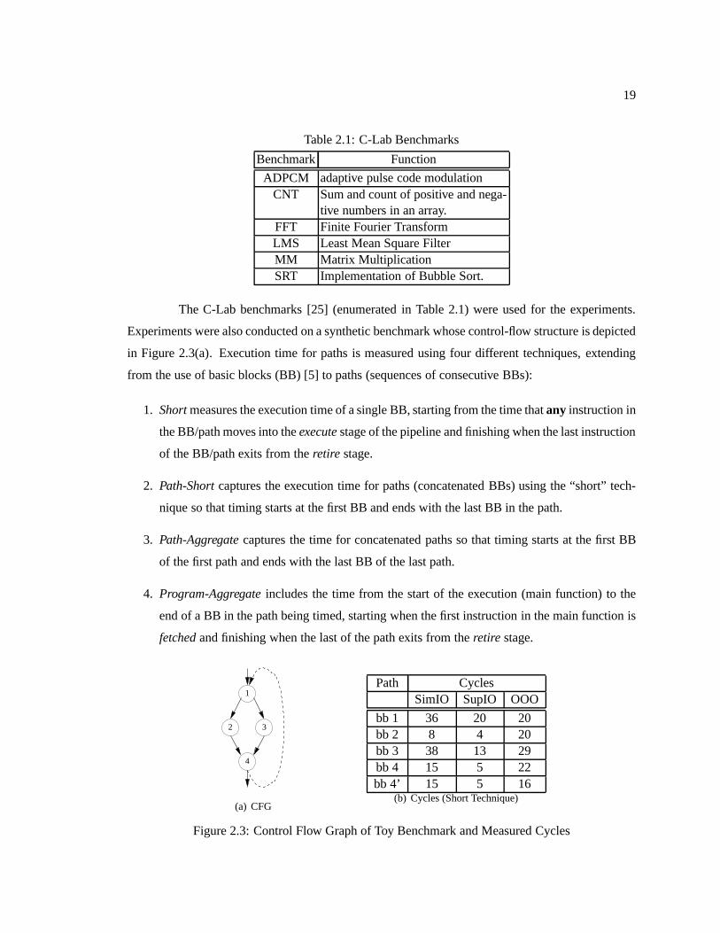
Table 2.1: C-Lab Benchmarks

Benchmark Function

ADPCM adaptive pulse code modulationCNT Sum and count of positive and nega-

tive numbers in an array.FFT Finite Fourier TransformLMS Least Mean Square FilterMM Matrix MultiplicationSRT Implementation of Bubble Sort.

The C-Lab benchmarks [25] (enumerated in Table 2.1) were used for the experiments.

Experiments were also conducted on a synthetic benchmark whose control-flow structure is depicted

in Figure 2.3(a). Execution time for paths is measured usingfour different techniques, extending

from the use of basic blocks (BB) [5] to paths (sequences of consecutive BBs):

1. Shortmeasures the execution time of a single BB, starting from thetime thatany instruction in

the BB/path moves into theexecutestage of the pipeline and finishing when the last instruction

of the BB/path exits from theretire stage.

2. Path-Shortcaptures the execution time for paths (concatenated BBs) using the “short” tech-

nique so that timing starts at the first BB and ends with the last BB in the path.

3. Path-Aggregatecaptures the time for concatenated paths so that timing starts at the first BB

of the first path and ends with the last BB of the last path.

4. Program-Aggregateincludes the time from the start of the execution (main function) to the

end of a BB in the path being timed, starting when the first instruction in the main function is

fetchedand finishing when the last of the path exits from theretire stage.

1

2 3

4

(a) CFG

Path CyclesSimIO SupIO OOO

bb 1 36 20 20bb 2 8 4 20bb 3 38 13 29bb 4 15 5 22bb 4’ 15 5 16

(b) Cycles (Short Technique)

Figure 2.3: Control Flow Graph of Toy Benchmark and MeasuredCycles

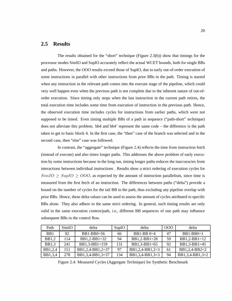
20

2.5 Results

The results obtained for the “short” technique (Figure 2.3(b)) show that timings for the

processor modes SimIO and SupIO accurately reflect the actual WCET bounds, both for single BBs

and paths. However, the OOO results exceed those of SupIO, due to early out-of-order execution of

some instructions in parallel with other instructions fromprior BBs in the path. Timing is started

when any instruction in the relevant path comes into the execute stage of the pipeline, which could

very well happen even when the previous path is not complete due to the inherent nature of out-of-

order execution. Since timing only stops when the last instruction in the current path retires, the

total execution time includes some time from execution of instruction in the previous path. Hence,

the observed execution time includes cycles for instructions from earlier paths, which were not

supposed to be timed. Even timing multiple BBs of a path in sequence (“path-short” technique)

does not alleviate this problem. bb4 and bb4’ represent the same code – the difference is the path

taken to get to basic block 4. In the first case, the “then” caseof the branch was selected and in the

second case, then “else” case was followed.

In contrast, the “aggregate” technique (Figure 2.4) reflects the time from instruction fetch

(instead of execute) and also times longer paths. This addresses the above problem of early execu-

tion by some instructions because in the long run, timing longer paths reduces the inaccuracies from

interactions between individual instructions . Results show a strict ordering of execution cycles for

SimIO ≥ SupIO ≥ OOO, as expected by the amount of instruction parallelism, since time is

measured from the first fetch of an instruction. The differences between paths (“delta”) provide a

bound on the number of cycles for the tail BB in the path, thus excluding any pipeline overlap with

prior BBs. Hence, these delta values can be used to assess theamount of cycles attributed to specific

BBs alone. They also adhere to the same strict ordering. In general, such timing results are only

valid in the same execution context/path,i.e., different BB sequences of one path may influence

subsequent BBs in the control flow.

Path SimIO delta SupIO delta OOO delta

BB1 82 BB1-BB0=56 66 BB1-BB 0=4 47 BB1-BB0=1BB1,2 114 BB1,2-BB1=32 94 BB1,2-BB1=28 59 BB1,2-BB1=12BB1,3 241 BB1,3-BB1=159 131 BB1,3-BB1=65 92 BB1,3-BB1=45

BB1,2,4 151 BB1,2,4-BB1,2=37 97 BB1,2,4-BB1,2=3 61 BB1,2,4-BB2=2BB1,3,4 278 BB1,3,4-BB1,3=37 134 BB1,3,4-BB1,3=3 94 BB1,3,4-BB1,3=2

Figure 2.4: Measured Cycles (Aggregate Technique) for Synthetic Benchmark

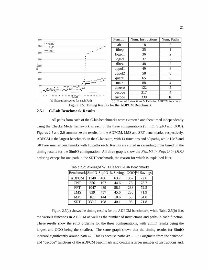
21

0

500

1000

1500

2000

2500

3000

3500

4000

1 4 7 10 13 16 19 22 25 28 31 34 37 40 43 46 49 52 55 58Path Id

Cycle

s

SimIOSupIOOOO

(a) Execution cycles for each Path

Function Num. Instructions Num. Paths

abs 18 2filtep 35 1

logsch 36 2logscl 37 2filtez 48 2

uppol1 49 8uppol2 58 8quantl 65 6main 88 4

upzero 122 5decode 317 4encode 330 16

(b) Num. of Instructions & Paths for ADPCM functionsFigure 2.5: Timing Results for the ADPCM Benchmark

2.5.1 C-Lab Benchmark Results

All paths from each of the C-lab benchmarks were extracted and then timed independently

using the CheckerMode framework in each of the three configurations (SimIO, SupIO and OOO).

Figures 2.5 and 2.6 summarize the results for the ADPCM, LMS and SRT benchmarks, respectively.

ADPCM is the largest benchmark in the C-lab suite, with14 functions and60 paths, while LMS and

SRT are smaller benchmarks with10 paths each. Results are sorted in ascending order based on the

timing results for the SimIO configuration. All three graphsshow theSimIO ≥ SupIO ≥ OOO

ordering except for one path in the SRT benchmark, the reasonfor which is explained later.

Table 2.2: Averaged WCECs for C-Lab Benchmarks

BenchmarkSimIO SupIO % SavingsOOO % Savings

ADPCM 1340 486 63.7 367 72.6CNT 356 197 44.6 76 78.7FFT 1047 439 58.1 288 72.5LMS 839 457 45.6 236 71.9MM 161 144 10.6 58 64.0SRT 330.2 198 40.1 93 71.8

Figure 2.5(a) shows the timing results for the ADPCM benchmark, while Table 2.5(b) lists

the various functions in ADPCM as well as the number of instructions and paths in each function.

These results show the strict ordering for the three configurations, with SimIO results being the

largest and OOO being the smallest. The same graph shows thatthe timing results for SimIO

increase significantly around path42. This is because paths42 − −61 originate from the “encode”

and “decode” functions of the ADPCM benchmark and contain a larger number of instructions and,

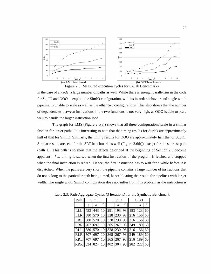
22

0

200

400

600

800

1000

1200

1400

1 2 3 4 5 6 7 8 9 10Path Id

Cyc

les

SimIOSupIOOOO

(a) LMS benchmark

0

100

200

300

400

500

600

700

800

1 2 3 4 5 6 7 8 9 10Path Id

Cyc

les

SimIOSupIOOOO

(b) SRT benchmarkFigure 2.6: Measured execution cycles for C-Lab Benchmarks

in the case ofencode, a large number of paths as well. While there is enough parallelism in the code

for SupIO and OOO to exploit, the SimIO configuration, with its in-order behavior and single width

pipeline, is unable to scale as well as the other two configurations. This also shows that the number

of dependencies between instructions in the two functions is not very high, as OOO is able to scale

well to handle the larger instruction load.

The graph for LMS (Figure 2.6(a)) shows that all three configurations scale in a similar

fashion for larger paths. It is interesting to note that the timing results for SupIO are approximately

half of that for SimIO. Similarly, the timing results for OOOare approximately half that of SupIO.

Similar results are seen for the SRT benchmark as well (Figure 2.6(b)), except for the shortest path

(path1). This path is so short that the effects described at the beginning of Section 2.5 become

apparent –i.e., timing is started when the first instruction of the program is fetched and stopped

when the final instruction is retired. Hence, the first instruction has to wait for a while before it is

dispatched. When the paths are very short, the pipeline contains a large number of instructions that

do not belong to the particular path being timed, hence bloating the results for pipelines with larger

width. The single width SimIO configuration does not suffer from this problem as the instruction is

Table 2.3: Path-Aggregate Cycles (3 Iterations) for the Synthetic Benchmark

Path SimIO SupIO OOO+ o δ + o δ + o δ

LLL 453 443 10 291 193 98 183 123 60LLR 580 570 10 328 230 98 216 156 60LRL 580 570 10 328 230 98 216 156 60LRR 707 697 10 365 267 98 249 189 60RLL 580 570 10 328 230 98 216 156 60RLR 707 697 10 365 267 98 249 189 60RRL 707 697 10 365 267 98 216 189 60RRR 834 824 10 402 304 98 282 222 60

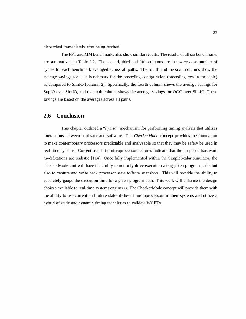
23

dispatched immediately after being fetched.

The FFT and MM benchmarks also show similar results. The results of all six benchmarks

are summarized in Table 2.2. The second, third and fifth columns are theworst-casenumber of

cycles for each benchmark averaged across all paths. The fourth and the sixth columns show the

average savings for each benchmark for the preceding configuration (preceding row in the table)

as compared to SimIO (column2). Specifically, the fourth column shows the average savingsfor

SupIO over SimIO, and the sixth column shows the average savings for OOO over SimIO. These

savings are based on the averages across all paths.

2.6 Conclusion

This chapter outlined a “hybrid” mechanism for performing timing analysis that utilizes

interactions between hardware and software. TheCheckerModeconcept provides the foundation

to make contemporary processors predictable and analyzable so that they may be safely be used in

real-time systems. Current trends in microprocessor features indicate that the proposed hardware

modifications are realistic [114]. Once fully implemented within the SimpleScalar simulator, the

CheckerMode unit will have the ability to not only drive execution along given program paths but

also to capture and write back processor state to/from snapshots. This will provide the ability to

accurately gauge the execution time for a given program path. This work will enhance the design

choices available to real-time systems engineers. The CheckerMode concept will provide them with

the ability to use current and future state-of-the-art microprocessors in their systems and utilize a

hybrid of static and dynamic timing techniques to validate WCETs.

24

Chapter 3

Merging State and Preserving Timing

Anomalies in Pipelines of High-End

Processors

3.1 Summary

This chapter provides further insights into the CheckerMode idea presented in Chapter 2

by introducing novel pipeline analysis techniques for accurately capturing the worst-case behavior

of real-time tasks,i.e., methods to capture (“snapshot”) pipeline state and to subsequently perform a

“merge” of previously captured snapshots. This chapter also includes proofs that the pipeline analy-

sis correctly preserves worst-case timing behavior on OOO processor pipelines. It also specifically

shows that anomalous pipeline effects, effectively dilating timing, are preserved by these methods.

3.2 Introduction

Chapter 2 introduced the notion of “hybrid” timing analysis[86] called theCheckerMode

infrastructure which combines the best features of both static and dynamic analysis to obtain accu-

rate WCET estimates for real-time tasks running on modern microprocessors. This chapter,

1. presents a more formal definition of the semantics of a snapshot;

2. explains how the information in a snapshot is obtained;

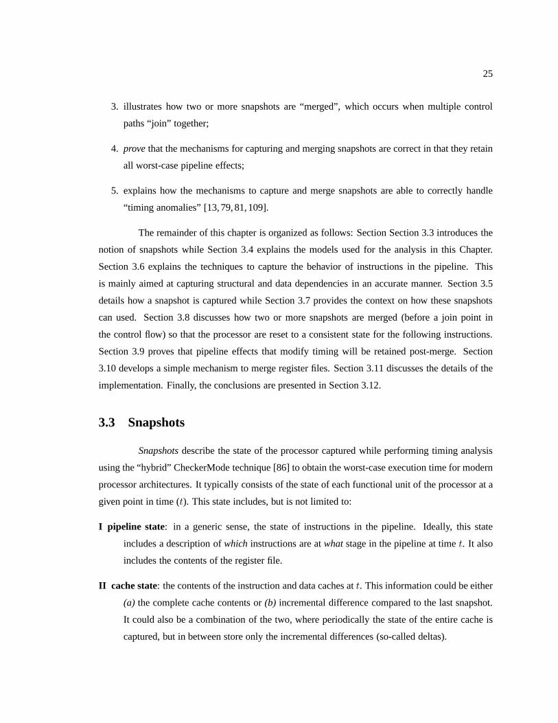
25

3. illustrates how two or more snapshots are “merged”, whichoccurs when multiple control

paths “join” together;

4. provethat the mechanisms for capturing and merging snapshots arecorrect in that they retain

all worst-case pipeline effects;

5. explains how the mechanisms to capture and merge snapshots are able to correctly handle

“timing anomalies” [13,79,81,109].

The remainder of this chapter is organized as follows: Section Section 3.3 introduces the

notion of snapshots while Section 3.4 explains the models used for the analysis in this Chapter.

Section 3.6 explains the techniques to capture the behaviorof instructions in the pipeline. This

is mainly aimed at capturing structural and data dependencies in an accurate manner. Section 3.5

details how a snapshot is captured while Section 3.7 provides the context on how these snapshots

can used. Section 3.8 discusses how two or more snapshots aremerged (before a join point in

the control flow) so that the processor are reset to a consistent state for the following instructions.

Section 3.9 proves that pipeline effects that modify timingwill be retained post-merge. Section

3.10 develops a simple mechanism to merge register files. Section 3.11 discusses the details of the

implementation. Finally, the conclusions are presented inSection 3.12.

3.3 Snapshots

Snapshotsdescribe the state of the processor captured while performing timing analysis

using the “hybrid” CheckerMode technique [86] to obtain theworst-case execution time for modern

processor architectures. It typically consists of the state of each functional unit of the processor at a

given point in time (t). This state includes, but is not limited to:

I pipeline state: in a generic sense, the state of instructions in the pipeline. Ideally, this state

includes a description ofwhich instructions are atwhatstage in the pipeline at timet. It also

includes the contents of the register file.

II cache state: the contents of the instruction and data caches att. This information could be either

(a) the complete cache contents or(b) incremental difference compared to the last snapshot.

It could also be a combination of the two, where periodicallythe state of the entire cache is

captured, but in between store only the incremental differences (so-called deltas).

26

III branch predictor state : similar to the cache state above:(a) complete branch history register

and branch table contents;(b) delta from previous snapshot; or(c) a combination of the two.

IV your favorite processor unit : state from any additional/future processor units that needs to be

captured to accurately characterize the worst-case behavior of the processor.

This chapter focuses on capturing thepipeline information of the processor for snapshots

and not on caches, branch predictors,etc. Analysis of instruction caches is a solved problem, and

any such analysis can be plugged into the CheckerMode framework to obtain better worst-case

results. Analysis of data caches is a hard problem but some analysis does exist [93, 104, 123, 131],

results from which can also be inserted into the CheckerModeframework to tighten the WCET

results. Branch Predictor analysis is left for future work.

While capturing fine-grained details of instruction flow through the pipeline (defined

above as “pipeline state”) would be ideal, practical difficulties prevent the process. Many changes

to the design and implementation of the processor will have to be carried out to attain the ability

to observe every single stage of the pipeline, instructionsin flight, data forwarding, etc. Hence

this chapter presents a novel technique devised to capture pipeline information, which, in essence,

achieves the effect of characterizing the state of the pipeline at the given instant. This technique is

named, the “drain-retire” (DR) technique. The DR techniqueis based on the idea that the only point

of predictability in an out-of-order pipeline is at the retire stage. Since retire happensin-order, one

can be sure that the retire order of instructions is deterministic. The DR technique is discussed in

more detail in Sections 3.5 and 3.7.

3.4 Analysis Model

Figure 3.1(a) shows a section of the instruction stream thatis executing through the

pipeline. LetSn be the last snapshot that was captured. Let “max” be the maximum number

of instructions that can fit into the pipeline assuming that there are no dependencies between any of

them. This is the theoretical upper bound for the pipeline capacity and is typically never achieved

in practice – due to the existence of dependencies between instructions, which introduce bubbles in

the pipeline.

If r is the most recent instruction that was fetched into the pipeline, then letp be the

instruction that was issuedmax cycles earlier in the instruction stream. Hence,p is the farthest

instruction in the stream that can directly affectr’s flow through the pipe. Instructions beforep have

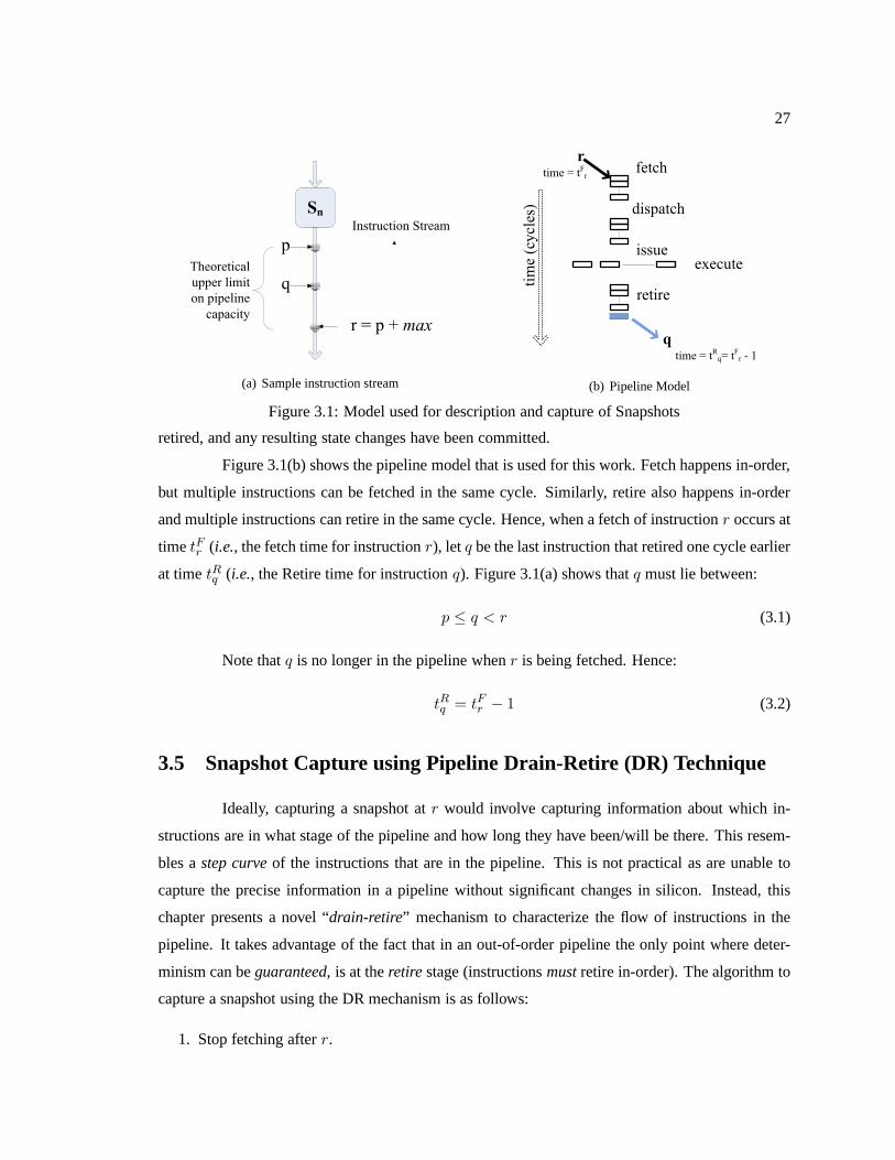
27

(a) Sample instruction stream (b) Pipeline Model

Figure 3.1: Model used for description and capture of Snapshots

retired, and any resulting state changes have been committed.

Figure 3.1(b) shows the pipeline model that is used for this work. Fetch happens in-order,

but multiple instructions can be fetched in the same cycle. Similarly, retire also happens in-order

and multiple instructions can retire in the same cycle. Hence, when a fetch of instructionr occurs at

timetFr (i.e., the fetch time for instructionr), letq be the last instruction that retired one cycle earlier

at timetRq (i.e., the Retire time for instructionq). Figure 3.1(a) shows thatq must lie between:

p ≤ q < r (3.1)

Note thatq is no longer in the pipeline whenr is being fetched. Hence:

tRq = tFr − 1 (3.2)

3.5 Snapshot Capture using Pipeline Drain-Retire (DR) Technique

Ideally, capturing a snapshot atr would involve capturing information about which in-

structions are in what stage of the pipeline and how long theyhave been/will be there. This resem-

bles astep curveof the instructions that are in the pipeline. This is not practical as are unable to

capture the precise information in a pipeline without significant changes in silicon. Instead, this

chapter presents a novel “drain-retire” mechanism to characterize the flow of instructions in the

pipeline. It takes advantage of the fact that in an out-of-order pipeline the only point where deter-

minism can beguaranteed, is at theretire stage (instructionsmustretire in-order). The algorithm to

capture a snapshot using the DR mechanism is as follows:

1. Stop fetching afterr.

28

2. StoretRq , the time whenq retired.

3. Let execution proceed through the pipeline untilr retires (i.e., the pipeline drains completely).

4. Track the retire time of every instruction fromq up until, and includingr (i.e., tRr ).

Figure 3.2 shows the results of applying the above algorithmto the model and instructions

described in Section 3.4. This figure shows the step curve obtained by tracking the retire times of

all instructions followingq until r retires.

Figure 3.2: Snapshot Captured using the DR Technique

The vertical axis represents time while the horizontal axisrepresents the instructions that

retire. Hence, the curve is bounded, in the time domain, bytRq and tRr with upper boundmax.

Unlike similar step curves for in-order pipelines, this curve is multi-dimensional. The horizontal

axis now encodes information about groups of instructions that retire together. As the figure shows,

the horizontal parts of the “step” directly represents the order and the number of instructions retiring

at that particular point in time (i.e., multiple instructions retiring in the same cycle).Note: theexact

order of instruction retirement at any given level must alsobe tracked. All of this information,

combined with the “state” of the reservation stations (Section 3.6), now forms a pipelinesnapshot,

which is formally defined in Figure 3.3.

3.6 Capturing Structural and Data Dependencies using Reservation

Stations

3.6.1 Structural Dependencies

Consider the situation shown in Figure 3.4(a). “a1” and “a2” are twomulti-cycleinstruc-

tions that require the same execution unit (fore.g., the “floating point multiply” unit). Assume that

there is only one instance of this type of execution unit in the pipeline. Now there exists astructural

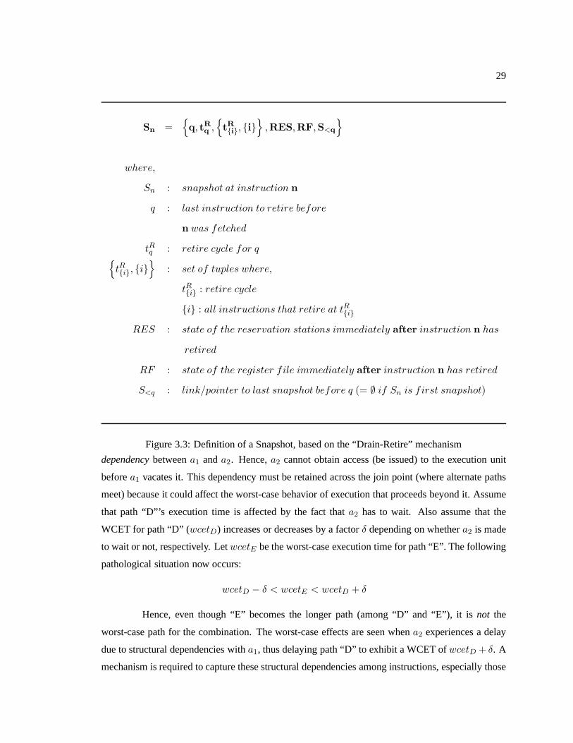
29

Sn ={

q, tRq ,{

tR{i}, {i}}

,RES,RF,S<q

}

where,

Sn : snapshot at instruction n

q : last instruction to retire before

n was fetched

tRq : retire cycle for q{

tR{i}, {i}}

: set of tuples where,

tR{i} : retire cycle

{i} : all instructions that retire at tR{i}

RES : state of the reservation stations immediately after instruction n has

retired

RF : state of the register file immediately after instruction n has retired

S<q : link/pointer to last snapshot before q (= ∅ if Sn is first snapshot)

Figure 3.3: Definition of a Snapshot, based on the “Drain-Retire” mechanism

dependencybetweena1 anda2. Hence,a2 cannot obtain access (be issued) to the execution unit

beforea1 vacates it. This dependency must be retained across the joinpoint (where alternate paths

meet) because it could affect the worst-case behavior of execution that proceeds beyond it. Assume

that path “D”’s execution time is affected by the fact thata2 has to wait. Also assume that the

WCET for path “D” (wcetD) increases or decreases by a factorδ depending on whethera2 is made

to wait or not, respectively. LetwcetE be the worst-case execution time for path “E”. The following

pathological situation now occurs:

wcetD − δ < wcetE < wcetD + δ

Hence, even though “E” becomes the longer path (among “D” and“E”), it is not the

worst-case path for the combination. The worst-case effects are seen whena2 experiences a delay

due to structural dependencies witha1, thus delaying path “D” to exhibit a WCET ofwcetD + δ. A

mechanism is required to capture these structural dependencies among instructions, especially those

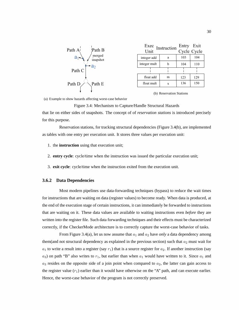
30

(a) Example to show hazards affecting worst-case behavior

(b) Reservation Stations

Figure 3.4: Mechanism to Capture/Handle Structural Hazards

that lie on either sides of snapshots. The concept of ofreservation stationsis introduced precisely

for this purpose.

Reservation stations, for tracking structural dependencies (Figure 3.4(b), are implemented

as tables with one entry per execution unit. It stores three values per execution unit:

1. theinstruction using that execution unit;

2. entry cycle: cycle/time when the instruction was issued the particularexecution unit;

3. exit cycle: cycle/time when the instruction exited from the executionunit.

3.6.2 Data Dependencies

Most modern pipelines use data-forwarding techniques (bypass) to reduce the wait times

for instructions that are waiting on data (register values)to become ready. When data is produced, at

the end of the execution stage of certain instructions, it can immediately be forwarded to instructions

that are waiting on it. These data values are available to waiting instructions evenbeforethey are

written into the register file. Such data forwarding techniques and their effects must be characterized

correctly, if the CheckerMode architecture is to correctlycapture the worst-case behavior of tasks.

From Figure 3.4(a), let us now assume thata1 anda2 haveonlya data dependency among

them(and not structural dependency as explained in the previous section) such thata2 must wait for

a1 to write a result into a register (sayr1) that is a source register fora2. If another instruction (say

a3) on path “B” also writes tor1, but earlier than whena1 would have written to it. Sincea1 and

a3 resides on the opposite side of a join point when compared toa2, the latter can gain access to

the register value (r1) earlier than it would have otherwise on the “A” path, and canexecute earlier.

Hence, the worst-case behavior of the program is not correctly preserved.

31

Reservation stations are also used for the register file to correctly track the data dependen-

cies between instructions and the time(s) when data becomesavailable and when they can be used

by dependent instructions. Each register now has an associated “reservation station” which stores

thelatestcycle when the register value was available (i.e. after the execution stage of the instruction

that produced that value).

Note: The process of writing information into the reservation stations isnoton the critical

path. Hence, it does not affect the execution of instructions in the pipeline.

3.7 Snapshot Usage

A snapshot captured using the DR technique in the previous section consists of informa-

tion about:

1. instructions

2. their order of retirement

3. cycles between retirement of instructions

4. the last instruction that retired (q) before the snapshot instruction (r).

This section elaborates the use of this information.

When execution must be restarted from a snapshot, instruction fetching must from instruc-

tion q because instructions that preceded it cannot directly affect the execution ofr. While fetch

can start fromq, there is no information about the processor state atq. Hence, the last snapshot

beforeq, which isSn, must be restored, as seen in Figure 3.1(a). To account for the worst case, the

start must actually be from the snapshot that precedes instructionp. Instructionp is the instruction

that is at the theoretical bound for the capacity of the pipeline, max, relative tor. If there exists a

snapshot betweenp andq, then the pessimism may be reduced by starting at the snapshot thatimme-

diatelyprecedesq since it is known that instructionq defines therealistic capacity of the pipeline.

Now information from this snapshot can be restored to bring the processor into a consistent state.

Fetching is restarted from the instruction that immediately follows Sn and execution is allowed to

proceed until the new/current snapshot,Sr (at instructionr), is reached. Once instructionq retires,

information about subsequent instructions is looked up from Sr to see how much time elapses, if

any, between their retirement. Each instruction starting fromr can now retire only after the requisite

number of cycles has elapsed, as determined by the information inSn. Hence, instructions can retire

32

at or after the number of cycles recordedfor it in the snapshot, butnever before. From Figure 3.2, it

is seen that two instructions followingq can retire at the same time, but no earlier than1 cycle after

q. The next instruction can only retire2 cycles after the previous2 instructions have retired, and so

on.

A similar process is employed for theissuestage of the pipeline. The reservation stations

are used to control what instructions are issued, when and into what execution unit. Figure 3.4(b),

shows that an instruction that wishes to use an execution unit (say the integer multiplier), cannot

gain access to it before cycle104, and once it has been given access, another instruction cannot

obtain it until the previous instruction exits (which, in this case, will be cycle110). This process

ensures that structural dependencies between instructions on either side of the snapshot are still

retained.

Similarly, instructions that depend on certain register values to be ready cannot proceed

with their execution until the cycle stored in that register’s reservation station comes to pass. This

ensures that instructions that have data dependencies among them still retain the correct dependency

information post-merge.

Hence, the semantic meaning associated with snapshots, initially constrained to static

aspects only, has been enhanced by dynamic information. This has an effect on the instruction

flow through the pipeline. Hence, a snapshot is now defined as information that affects the flow of

instructions through the pipeline when the “snapshot instruction” (r in the above case) is fetched.

Snapshots are able to affect the pipeline behavior by allowing instructions captured in them to

retire only with predetermined delays (i.e., at or after the retire times captured in the snapshot)

or gain access to execution units based on constraints enforced by the reservation stations,etc..

Modifications to the retire stage, mentioned in Section 3.5,as well as the issue stage (to look up the

reservation stations) are useful in aiding the process of restoring snapshots by providing the ability

to exercise fine control on when certain instructions (captured in the snapshot) are allowed to be

issued or to retire.

Note: This method of using snapshots and constraining instruction flow through the

pipeline can be achieved in one of two ways:

1. by enhancing thefetchstage of the pipeline so that finer control can be exercised onwhen

instructions are to be fetched and fromwherein the program flow

2. by insertingnop instructions to cover “bubbles” in the program flow.

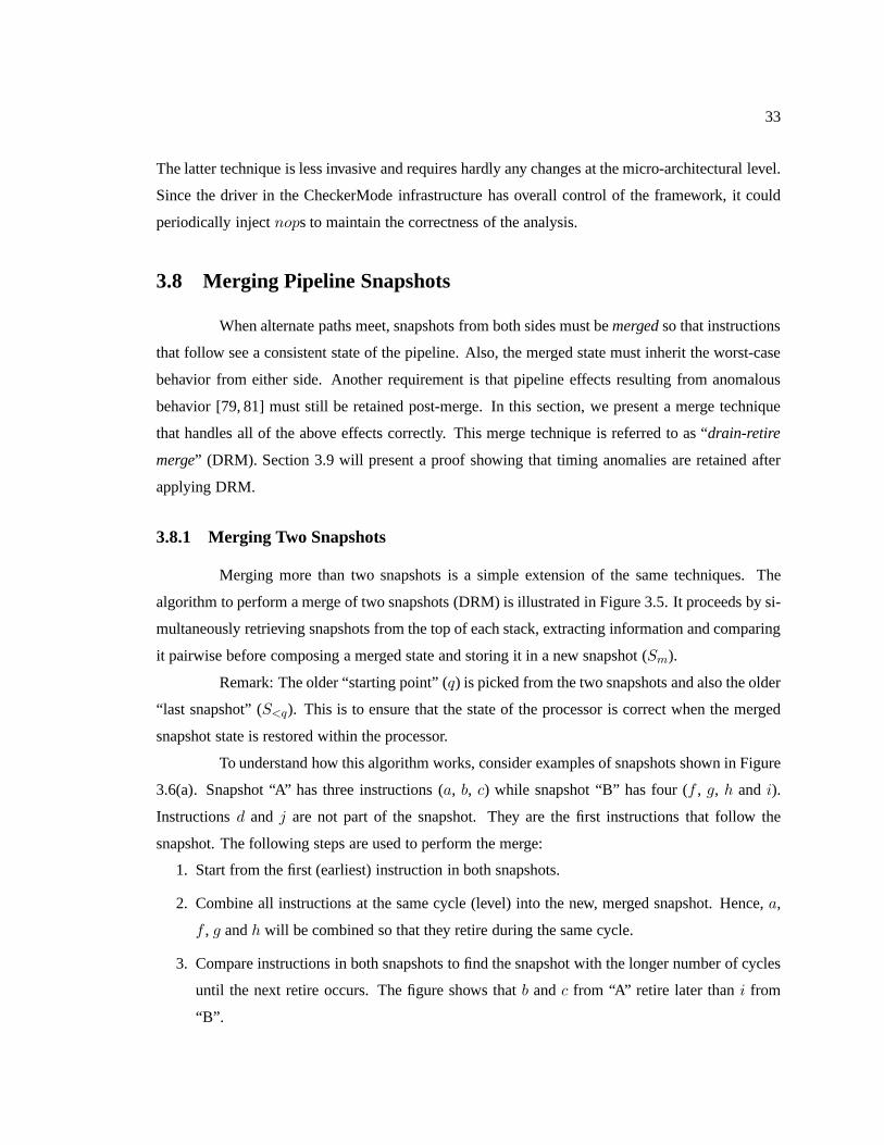
33

The latter technique is less invasive and requires hardly any changes at the micro-architectural level.

Since the driver in the CheckerMode infrastructure has overall control of the framework, it could

periodically injectnops to maintain the correctness of the analysis.

3.8 Merging Pipeline Snapshots

When alternate paths meet, snapshots from both sides must bemergedso that instructions

that follow see a consistent state of the pipeline. Also, themerged state must inherit the worst-case

behavior from either side. Another requirement is that pipeline effects resulting from anomalous

behavior [79, 81] must still be retained post-merge. In thissection, we present a merge technique

that handles all of the above effects correctly. This merge technique is referred to as “drain-retire

merge” (DRM). Section 3.9 will present a proof showing that timinganomalies are retained after

applying DRM.

3.8.1 Merging Two Snapshots

Merging more than two snapshots is a simple extension of the same techniques. The

algorithm to perform a merge of two snapshots (DRM) is illustrated in Figure 3.5. It proceeds by si-

multaneously retrieving snapshots from the top of each stack, extracting information and comparing

it pairwise before composing a merged state and storing it ina new snapshot (Sm).

Remark: The older “starting point” (q) is picked from the two snapshots and also the older

“last snapshot” (S<q). This is to ensure that the state of the processor is correctwhen the merged

snapshot state is restored within the processor.

To understand how this algorithm works, consider examples of snapshots shown in Figure

3.6(a). Snapshot “A” has three instructions (a, b, c) while snapshot “B” has four (f , g, h and i).

Instructionsd and j are not part of the snapshot. They are the first instructions that follow the

snapshot. The following steps are used to perform the merge:

1. Start from the first (earliest) instruction in both snapshots.

2. Combine all instructions at the same cycle (level) into the new, merged snapshot. Hence,a,

f , g andh will be combined so that they retire during the same cycle.

3. Compare instructions in both snapshots to find the snapshot with the longer number of cycles

until the next retire occurs. The figure shows thatb andc from “A” retire later thani from

“B”.

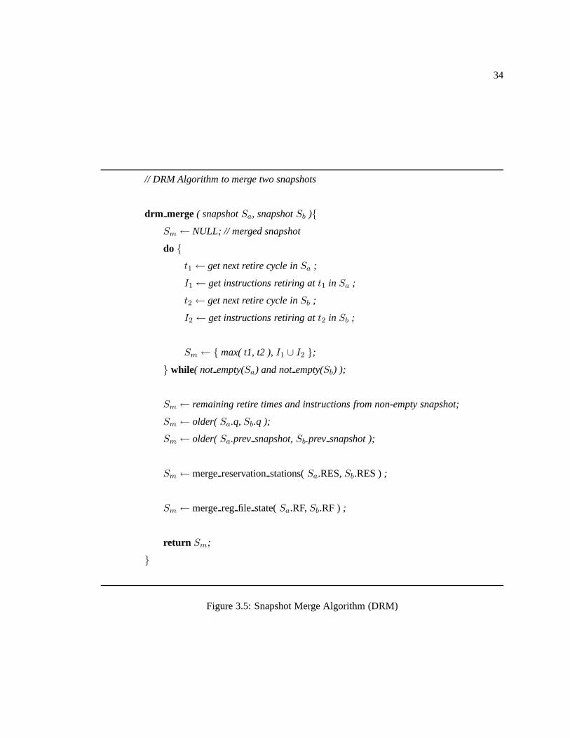
34

// DRM Algorithm to merge two snapshots

drm merge( snapshotSa, snapshotSb ){

Sm ← NULL; // merged snapshot

do {

t1 ← get next retire cycle inSa ;

I1 ← get instructions retiring att1 in Sa ;

t2 ← get next retire cycle inSb ;

I2 ← get instructions retiring att2 in Sb ;

Sm ← {max( t1, t2 ),I1 ∪ I2 };

} while( not empty(Sa) and notempty(Sb) );

Sm ← remaining retire times and instructions from non-empty snapshot;

Sm ← older( Sa.q,Sb.q );

Sm ← older( Sa.prev snapshot,Sb.prev snapshot );

Sm ←mergereservationstations(Sa.RES,Sb.RES );

Sm ←mergereg file state(Sa.RF,Sb.RF ) ;

return Sm;

}

Figure 3.5: Snapshot Merge Algorithm (DRM)

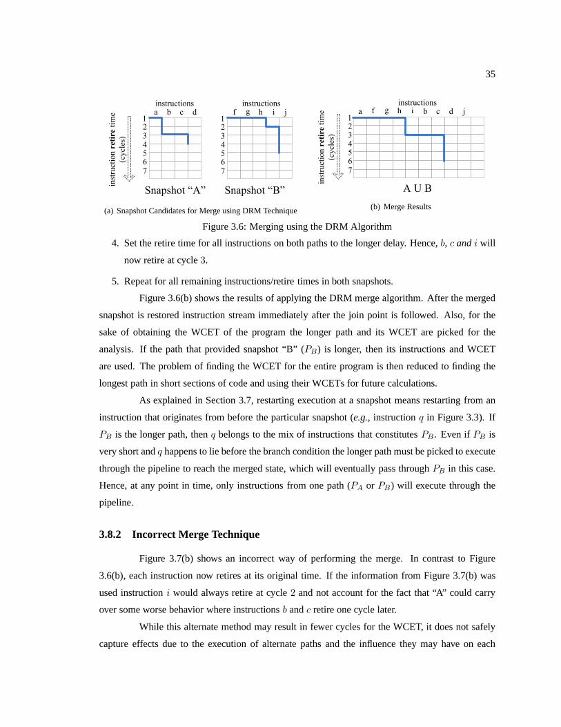
35

(a) Snapshot Candidates for Merge using DRM Technique (b) Merge Results

Figure 3.6: Merging using the DRM Algorithm

4. Set the retire time for all instructions on both paths to the longer delay. Hence,b, c andi will

now retire at cycle3.

5. Repeat for all remaining instructions/retire times in both snapshots.

Figure 3.6(b) shows the results of applying the DRM merge algorithm. After the merged

snapshot is restored instruction stream immediately afterthe join point is followed. Also, for the

sake of obtaining the WCET of the program the longer path and its WCET are picked for the

analysis. If the path that provided snapshot “B” (PB) is longer, then its instructions and WCET

are used. The problem of finding the WCET for the entire program is then reduced to finding the

longest path in short sections of code and using their WCETs for future calculations.

As explained in Section 3.7, restarting execution at a snapshot means restarting from an

instruction that originates from before the particular snapshot (e.g., instructionq in Figure 3.3). If

PB is the longer path, thenq belongs to the mix of instructions that constitutesPB . Even ifPB is

very short andq happens to lie before the branch condition the longer path must be picked to execute

through the pipeline to reach the merged state, which will eventually pass throughPB in this case.

Hence, at any point in time, only instructions from one path (PA or PB) will execute through the

pipeline.

3.8.2 Incorrect Merge Technique

Figure 3.7(b) shows an incorrect way of performing the merge. In contrast to Figure

3.6(b), each instruction now retires at its original time. If the information from Figure 3.7(b) was

used instructioni would always retire at cycle2 and not account for the fact that “A” could carry

over some worse behavior where instructionsb andc retire one cycle later.

While this alternate method may result in fewer cycles for the WCET, it does not safely

capture effects due to the execution of alternate paths and the influence they may have on each

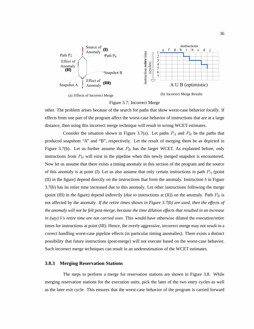
36

(a) Effects of Incorrect Merge (b) Incorrect Merge Results

Figure 3.7: Incorrect Merge

other. The problem arises because of the search for paths that show worst-case behaviorlocally. If

effects from one part of the program affect the worst-case behavior of instructions that are at a large

distance, then using this incorrect merge technique will result in wrong WCET estimates.

Consider the situation shown in Figure 3.7(a). Let pathsPA andPB be the paths that

produced snapshots “A” and “B”, respectively. Let the result of merging them be as depicted in

Figure 3.7(b). Let us further assume thatPB has the larger WCET. As explained before, only

instructions fromPB will exist in the pipeline when this newly merged snapshot isencountered.

Now let us assume that there exists a timing anomaly in this section of the program and the source

of this anomaly is at point (I). Let us also assume that only certain instructions in pathPA (point

(II) in the figure) depend directly on the instructions that form the anomaly. Instructionb in Figure

3.7(b) has its retire time increased due to this anomaly. Letother instructions following the merge

(point (III) in the figure) depend indirectly (due to instructions at (II)) on the anomaly. PathPB is

not affected by the anomaly.If the retire times shown in Figure 3.7(b) are used, then the effects of

the anomaly will not be felt post-merge, because the time dilation effects that resulted in an increase

in (say)b’s retire time are not carried over.This would have otherwise dilated the execution/retire

times for instructions at point (III). Hence, the overly aggressive, incorrect merge may not result in a

correct handling worst-case pipeline effects (in particular timing anomalies). There exists a distinct

possibility that future instructions (post-merge) will not execute based on the worst-case behavior.

Such incorrect merge techniques can result in an underestimation of the WCET estimates.

3.8.3 Merging Reservation Stations

The steps to perform a merge for reservation stations are shown in Figure 3.8. While

merging reservation stations for the execution units, pickthe later of the two entry cycles as well

as the later exit cycle. This ensures that the worst-case behavior of the program is carried forward

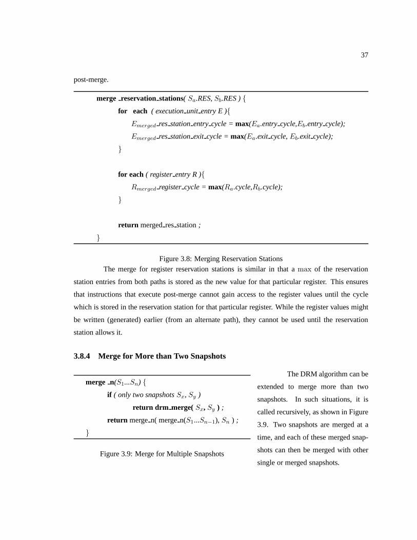
37

post-merge.

merge reservation stations( Sa.RES,Sb.RES ){

for each ( executionunit entry E ){

Emerged res station entry cycle =max(Ea.entry cycle,Eb.entry cycle);

Emerged res station exit cycle =max(Ea.exit cycle,Eb.exit cycle);

}

for each ( register entry R ){

Rmerged register cycle =max(Ra.cycle,Rb.cycle);

}

return mergedresstation;

}

Figure 3.8: Merging Reservation StationsThe merge for register reservation stations is similar in that a max of the reservation

station entries from both paths is stored as the new value forthat particular register. This ensures

that instructions that execute post-merge cannot gain access to the register values until the cycle

which is stored in the reservation station for that particular register. While the register values might

be written (generated) earlier (from an alternate path), they cannot be used until the reservation

station allows it.

3.8.4 Merge for More than Two Snapshots

merge n(S1...Sn) {

if ( only two snapshotsSx, Sy )

return drm merge(Sx, Sy ) ;

return mergen( mergen(S1...Sn−1), Sn ) ;

}

Figure 3.9: Merge for Multiple Snapshots

The DRM algorithm can be

extended to merge more than two

snapshots. In such situations, it is

called recursively, as shown in Figure

3.9. Two snapshots are merged at a

time, and each of these merged snap-

shots can then be merged with other

single or merged snapshots.

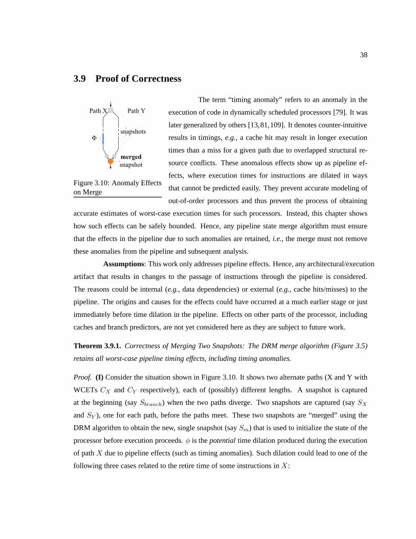
38

3.9 Proof of Correctness

Figure 3.10: Anomaly Effectson Merge

The term “timing anomaly” refers to an anomaly in the

execution of code in dynamically scheduled processors [79]. It was

later generalized by others [13,81,109]. It denotes counter-intuitive

results in timings,e.g., a cache hit may result in longer execution

times than a miss for a given path due to overlapped structural re-

source conflicts. These anomalous effects show up as pipeline ef-

fects, where execution times for instructions are dilated in ways

that cannot be predicted easily. They prevent accurate modeling of

out-of-order processors and thus prevent the process of obtaining

accurate estimates of worst-case execution times for such processors. Instead, this chapter shows

how such effects can be safely bounded. Hence, any pipeline state merge algorithm must ensure

that the effects in the pipeline due to such anomalies are retained,i.e., the merge must not remove

these anomalies from the pipeline and subsequent analysis.

Assumptions: This work only addresses pipeline effects. Hence, any architectural/execution

artifact that results in changes to the passage of instructions through the pipeline is considered.

The reasons could be internal (e.g., data dependencies) or external (e.g., cache hits/misses) to the

pipeline. The origins and causes for the effects could have occurred at a much earlier stage or just

immediately before time dilation in the pipeline. Effects on other parts of the processor, including

caches and branch predictors, are not yet considered here asthey are subject to future work.

Theorem 3.9.1.Correctness of Merging Two Snapshots: The DRM merge algorithm (Figure 3.5)

retains all worst-case pipeline timing effects, includingtiming anomalies.

Proof. (I) Consider the situation shown in Figure 3.10. It shows two alternate paths (X and Y with

WCETsCX and CY respectively), each of (possibly) different lengths. A snapshot is captured

at the beginning (saySbranch) when the two paths diverge. Two snapshots are captured (saySX

andSY ), one for each path, before the paths meet. These two snapshots are “merged” using the

DRM algorithm to obtain the new, single snapshot (saySm) that is used to initialize the state of the

processor before execution proceeds.φ is thepotentialtime dilation produced during the execution

of pathX due to pipeline effects (such as timing anomalies). Such dilation could lead to one of the

following three cases related to the retire time of some instructions inX:

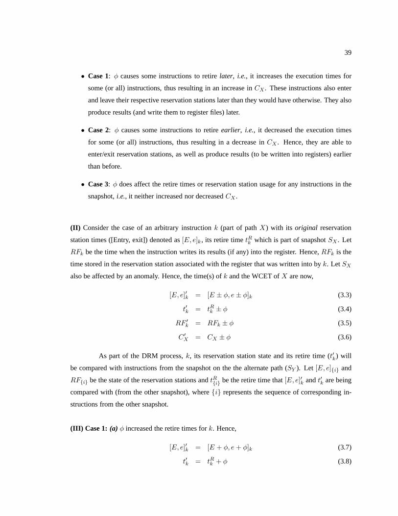
39

• Case 1: φ causes some instructions to retirelater, i.e., it increases the execution times for

some (or all) instructions, thus resulting in an increase inCX . These instructions also enter

and leave their respective reservation stations later thanthey would have otherwise. They also

produce results (and write them to register files) later.

• Case 2: φ causes some instructions to retireearlier, i.e., it decreased the execution times

for some (or all) instructions, thus resulting in a decreasein CX . Hence, they are able to

enter/exit reservation stations, as well as produce results (to be written into registers) earlier

than before.

• Case 3: φ does affect the retire times or reservation station usage for any instructions in the

snapshot,i.e., it neither increased nor decreasedCX .

(II) Consider the case of an arbitrary instructionk (part of pathX) with its original reservation

station times ([Entry, exit]) denoted as[E, e]k , its retire timetRk which is part of snapshotSX . Let

RFk be the time when the instruction writes its results (if any) into the register. Hence,RFk is the

time stored in the reservation station associated with the register that was written into byk. Let SX

also be affected by an anomaly. Hence, the time(s) ofk and the WCET ofX are now,

[E, e]′k = [E ± φ, e± φ]k (3.3)

t′k = tRk ± φ (3.4)

RF ′k = RFk ± φ (3.5)

C ′X = CX ± φ (3.6)

As part of the DRM process,k, its reservation station state and its retire time (t′k) will

be compared with instructions from the snapshot on the the alternate path (SY ). Let [E, e]{i} and

RF{i} be the state of the reservation stations andtR{i} be the retire time that[E, e]′k andt′k are being

compared with (from the other snapshot), where{i} represents the sequence of corresponding in-

structions from the other snapshot.

(III) Case 1: (a) φ increased the retire times fork. Hence,

[E, e]′k = [E + φ, e + φ]k (3.7)

t′k = tRk + φ (3.8)

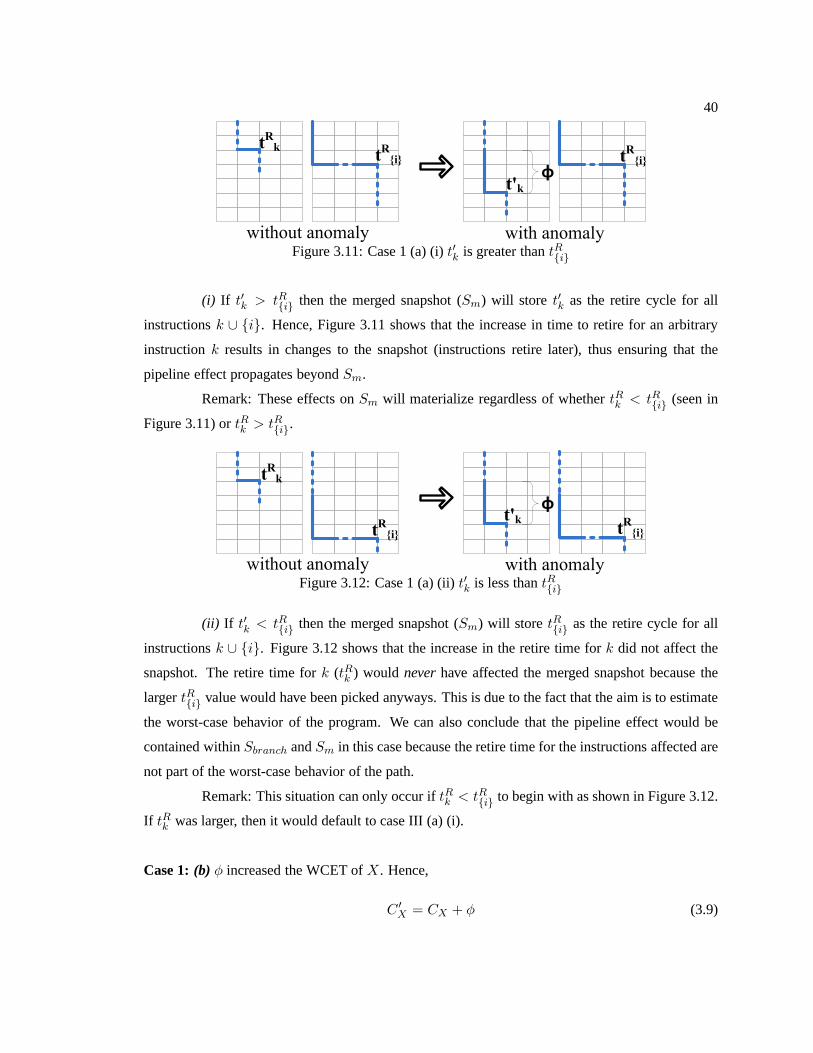
40

Figure 3.11: Case 1 (a) (i)t′k is greater thantR{i}

(i) If t′k > tR{i} then the merged snapshot (Sm) will store t′k as the retire cycle for all

instructionsk ∪ {i}. Hence, Figure 3.11 shows that the increase in time to retirefor an arbitrary

instructionk results in changes to the snapshot (instructions retire later), thus ensuring that the

pipeline effect propagates beyondSm.

Remark: These effects onSm will materialize regardless of whethertRk < tR{i} (seen in

Figure 3.11) ortRk > tR{i}.

Figure 3.12: Case 1 (a) (ii)t′k is less thantR{i}

(ii) If t′k < tR{i} then the merged snapshot (Sm) will store tR{i} as the retire cycle for all

instructionsk ∪ {i}. Figure 3.12 shows that the increase in the retire time fork did not affect the

snapshot. The retire time fork (tRk ) would neverhave affected the merged snapshot because the

largertR{i} value would have been picked anyways. This is due to the fact that the aim is to estimate

the worst-case behavior of the program. We can also concludethat the pipeline effect would be

contained withinSbranch andSm in this case because the retire time for the instructions affected are

not part of the worst-case behavior of the path.

Remark: This situation can only occur iftRk < tR{i} to begin with as shown in Figure 3.12.

If tRk was larger, then it would default to case III (a) (i).

Case 1:(b) φ increased the WCET ofX. Hence,

C ′X = CX + φ (3.9)

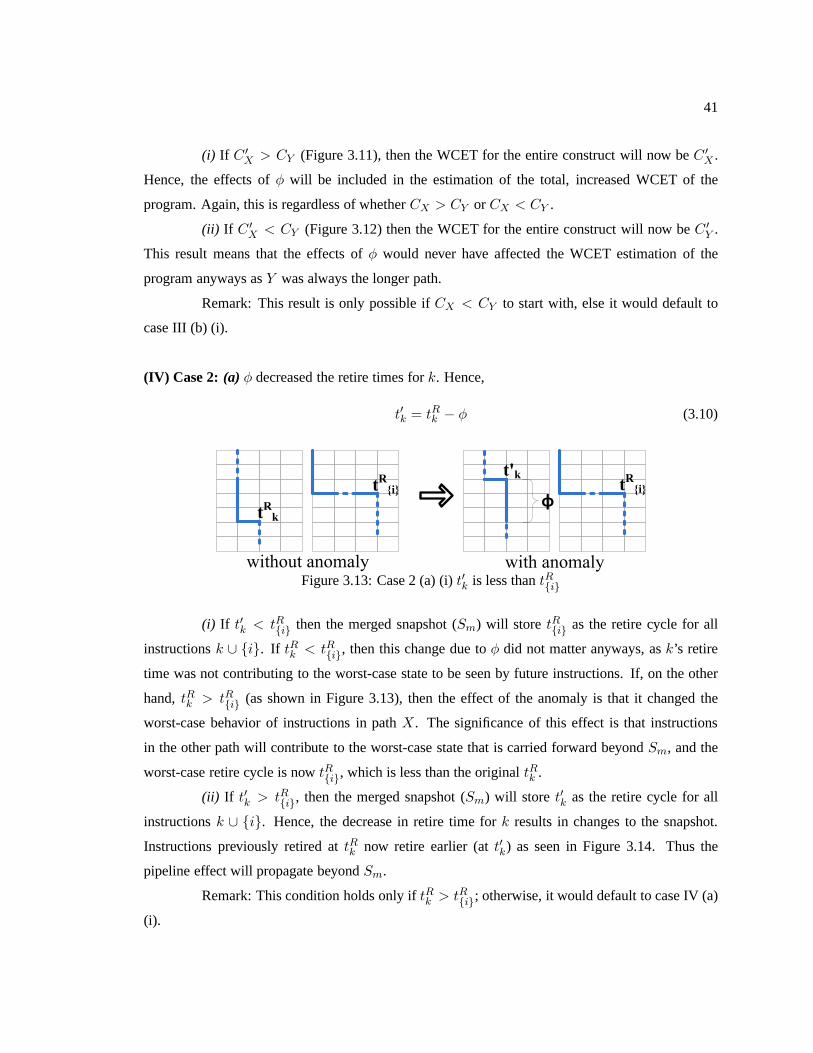
41

(i) If C ′X > CY (Figure 3.11), then the WCET for the entire construct will now beC ′

X .

Hence, the effects ofφ will be included in the estimation of the total, increased WCET of the

program. Again, this is regardless of whetherCX > CY or CX < CY .

(ii) If C ′X < CY (Figure 3.12) then the WCET for the entire construct will nowbeC ′

Y .

This result means that the effects ofφ would never have affected the WCET estimation of the

program anyways asY was always the longer path.

Remark: This result is only possible ifCX < CY to start with, else it would default to

case III (b) (i).

(IV) Case 2: (a) φ decreased the retire times fork. Hence,

t′k = tRk − φ (3.10)

Figure 3.13: Case 2 (a) (i)t′k is less thantR{i}

(i) If t′k < tR{i} then the merged snapshot (Sm) will store tR{i} as the retire cycle for all

instructionsk ∪ {i}. If tRk < tR{i}, then this change due toφ did not matter anyways, ask’s retire

time was not contributing to the worst-case state to be seen by future instructions. If, on the other

hand,tRk > tR{i} (as shown in Figure 3.13), then the effect of the anomaly is that it changed the

worst-case behavior of instructions in pathX. The significance of this effect is that instructions

in the other path will contribute to the worst-case state that is carried forward beyondSm, and the

worst-case retire cycle is nowtR{i}, which is less than the originaltRk .

(ii) If t′k > tR{i}, then the merged snapshot (Sm) will store t′k as the retire cycle for all

instructionsk ∪ {i}. Hence, the decrease in retire time fork results in changes to the snapshot.

Instructions previously retired attRk now retire earlier (att′k) as seen in Figure 3.14. Thus the

pipeline effect will propagate beyondSm.

Remark: This condition holds only iftRk > tR{i}; otherwise, it would default to case IV (a)

(i).

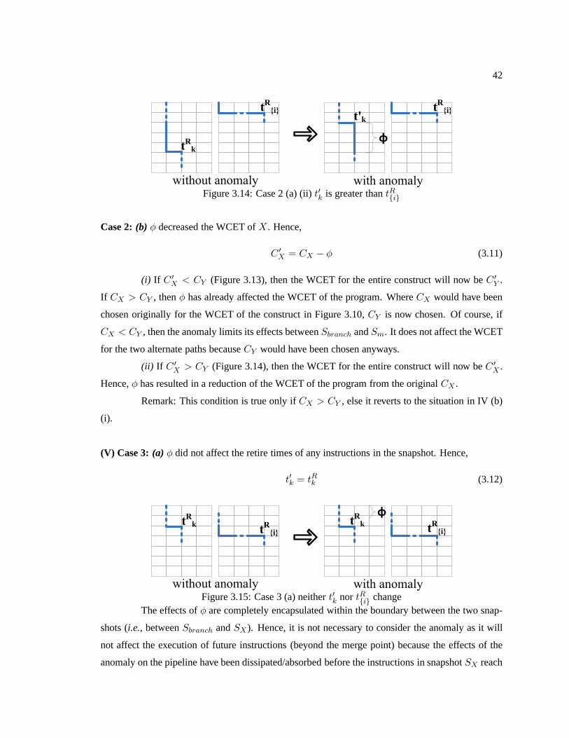
42

Figure 3.14: Case 2 (a) (ii)t′k is greater thantR{i}

Case 2:(b) φ decreased the WCET ofX. Hence,

C ′X = CX − φ (3.11)

(i) If C ′X < CY (Figure 3.13), then the WCET for the entire construct will now beC ′

Y .

If CX > CY , thenφ has already affected the WCET of the program. WhereCX would have been

chosen originally for the WCET of the construct in Figure 3.10, CY is now chosen. Of course, if

CX < CY , then the anomaly limits its effects betweenSbranch andSm. It does not affect the WCET

for the two alternate paths becauseCY would have been chosen anyways.

(ii) If C ′X > CY (Figure 3.14), then the WCET for the entire construct will now beC ′

X .

Hence,φ has resulted in a reduction of the WCET of the program from theoriginal CX .

Remark: This condition is true only ifCX > CY , else it reverts to the situation in IV (b)

(i).

(V) Case 3:(a) φ did not affect the retire times of any instructions in the snapshot. Hence,

t′k = tRk (3.12)

Figure 3.15: Case 3 (a) neithert′k nor tR{i} changeThe effects ofφ are completely encapsulated within the boundary between the two snap-

shots (i.e., betweenSbranch andSX). Hence, it is not necessary to consider the anomaly as it will

not affect the execution of future instructions (beyond themerge point) because the effects of the

anomaly on the pipeline have been dissipated/absorbed before the instructions in snapshotSX reach

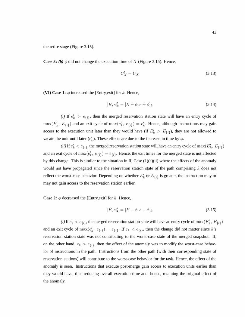
43

the retire stage (Figure 3.15).

Case 3:(b) φ did not change the execution time ofX (Figure 3.15). Hence,

C ′X = CX (3.13)

(VI) Case 1: φ increased the [Entry,exit] fork. Hence,

[E, e]′k = [E + φ, e + φ]k (3.14)

(i) If e′k > e{i}, then the merged reservation station state will have an entry cycle of

max(E′k, E{i}) and an exit cycle ofmax(e′k, e{i}) = e′k. Hence, although instructions may gain

access to the execution unit later than they would have (ifE′k > E{i}), they are not allowed to

vacate the unit until later (e′k). These effects are due to the increase in time byφ.

(ii) If e′k < e{i}, the merged reservation station state will have an entry cycle ofmax(E′k, E{i})

and an exit cycle ofmax(e′k, e{i}) = e{i}. Hence, the exit times for the merged state is not affected

by this change. This is similar to the situation in II, Case (1)(a)(ii) where the effects of the anomaly

would not have propagated since the reservation station state of the path comprisingk does not

reflect the worst-case behavior. Depending on whetherE′k or E{i} is greater, the instruction may or

may not gain access to the reservation station earlier.

Case 2:φ decreased the [Entry,exit] fork. Hence,

[E, e]′k = [E − φ, e− φ]k (3.15)

(i) If e′k < e{i}, the merged reservation station state will have an entry cycle ofmax(E′k, E{i})

and an exit cycle ofmax(e′k, e{i}) = e{i}. If ek < e{i}, then the change did not matter sincek’s

reservation station state was not contributing to the worst-case state of the merged snapshot. If,

on the other hand,ek > e{i}, then the effect of the anomaly was to modify the worst-case behav-

ior of instructions in the path. Instructions from the otherpath (with their corresponding state of

reservation stations) will contribute to the worst-case behavior for the task. Hence, the effect of the

anomaly is seen. Instructions that execute post-merge gainaccess to execution units earlier than

they would have, thus reducing overall execution time and, hence, retaining the original effect of

the anomaly.

44

Instructions that are a part of the snapshot also gain accessto the reservation stations at a

later time, depending on whetherE′k or E{i} is greater.

(ii) If e′k > e{i}, the effect of the anomaly was to reduce the time taken for instructions to

be issued to execution units. The state of the merged reservation station will be,[max(E′k, E{i}), e′k].

Without reservation stations, instructions would have been able to exit from the execution units at

ek. Due to the presence of reservation stations, they now exit at time e′k < ek. Hence, the effect of

the anomaly in reducing the execution time is carried forward beyond the merge.

(VII) Case 1: φ increased theRF entry fork. Hence,

RF ′k = RFk + φ (3.16)

(i) If RF ′k > RF{i}, then the merged register reservation station state will store the value,

RF ′k. Hence, instructions that depend on the register corresponding to RF will gain access to the

execution unitlater than they would have due to the increase in time byφ.

(ii) If RF ′k < RF{i}, the merged register reservation station state will will store the value

RF{i}. This is similar to the situation in II, Case (1)(a)(ii) and VI Case (1) (a) (ii), where the effects

of the anomaly would not have propagated since the register reservation station state of the path

comprisingk does not reflect the true worst-case behavior.

Case 2:φ decreased theRF for k. Hence,

RF ′k = RFk − φ (3.17)

(i) If RF ′k < RF{i}, the merged register reservation station state will have a cycle of

RF{i}. If RFk < RF{i}, then the change did not matter sincek’s register reservation station

state was not contributing to the worst-case state of the merged snapshot. If, on the other hand,

RFk > RF{i}, then the effect of the anomaly was to modify the worst-case behavior of instructions

in the path. Instructions from the other path (with their corresponding state of reservation stations)

will contribute to the worst-case behavior for the task. Hence, the effect of the anomaly is seen.

Instructions that execute post-merge are allowed to accessthe data written into the register file

earlier than they would have, thus reducing overall execution time hence retaining the original effect

of the anomaly.

(ii) If RF ′k > RF{i}, the effect of the anomaly was to reduce the time taken for instruc-

tions to gain access to the data (they depend on) from the register file. The state of the merged

45

register reservation station will be,RF ′k. Without register reservation stations, instructions would

have been able to read the required data values atRFk. Due to the presence of reservation stations,

they now get the required inputs (from the register) atRF ′k < RFk. Hence, the effect of the anomaly

in reducing the execution time is carried forward beyond themerge.

Cases (I) – (VII) proved that pipeline effects due to timing anomalies (or other pipeline

effects) will be retained post-merge if the merge is based onthe DRM algorithm. If the pipeline

effects resulted in increases or decreases (execution time/retire cycles/etc.), then these effects are

carried over if these effects changed the worst-case behavior of the path. Hence, this proof holds for

merging anytwo snapshots.

Theorem 3.9.2.Correctness of Merging Multiple Snapshots: The algorithm in Figure 3.9 is correct

with respect to preserving worst-case timing effects in thepipeline when merging multiple snapshots.

Proof. The DRM algorithm is effectively applied recursively to perform merges on multiple snap-

shots. The “drmmerge” algorithm is called ontwo snapshots at a time to obtain a merged state,

which is then merged with the next snapshot and so on. This chapter has shown above that pipeline

effects are not lost when merging two snapshots at a time. Since merging multiple snapshots occurs

two at a time, one can infer that the pipeline effects will be retained across merging multiple snap-

shots if the said effects alter the worst-case behavior of the paths. Hence, the proof hold true for

merging an arbitrary number of snapshots.

3.10 Merging Register Files

To perform a merge on the register file state (“RF” from Figure3.3) a simple technique is

applied to each register:

• If the register value isunchangedacross the snapshots, then the merged state will retain that

value in the register;

• If the register value isdifferent, then set the merged value to a Not-A-Number (NaN ) [86].

This is to handle values that are input-dependent which willnot be known until run-time.

This is safe due to the conservative semantics of any operation of NaN that, by definition, re-

sults in a conservative value (NaN unless trivial arithmetic rules apply, such as multiplication

with zero) and in conservative temporal requirements (worst-case number of cycles for this

operation under the given operands).

46

Performing the above checks/modifications on every register in the register file in both

snapshots allows easy construction of a new “merged” state for the register file.Note: a merge on

register files deals with the actual register values. This isdifferent from merging reservation stations

for register files (Section 3.8.3).

The ability to extract and/or write back register file state can be realized by simple mod-

ifications of existing microarchitecture features,i.e., the Precise Event-Based Sampling (PEBS)

with user-selected access to selected shadow buffers [114]present in the Intel X86 architecture.

The CheckerMode design makes buffers used in this and other architectural techniques uniformly

available to the user.

3.11 Implementation

TheCheckerModeinfrastructure has been implemented on an enhancedSimpleScalarpro-

cessor simulation framework [21]. It has the ability to model a variety of processor configurations

(SMT, CMP,etc.). The previous chapter (Chapter 2) illustrated how the simulator was enhanced

by adding the ability to start/stop execution at given arbitrary program counter (PC) values as well

as the ability to capture timing information for the given range of PCs. It has now been further

modified to include the process of capturing the state of the processor during theissuestage (i.e.,

using the concept of reservation stations introduced in this chapter). It also includes the ability to

capture and merge snapshots and to reset the state of the the pipeline to a given snapshot as detailed

in this paper.

3.12 Conclusion

This chapter outlined a sophisticated pipeline analysis scheme that is able to estimate the

worst-case behavior of out-of-order pipelines in asafemanner. It also showed that CheckerMode

is able to correctly deal with timing anomalies and has the ability to conduct the analysis in ways

that are minimally invasive with respect to the processor. More specifically, minor changes to ex-

isting micro-architectural features are suggested, that extend contemporary monitoring techniques

already present in hardware. This analysis, when integrated with the CheckerMode infrastructure,

utilizes interactions between hardware and software to make contemporary processors predictable

and analyzable. Such processors may now be safely used in real-time systems, thus moving the

state-of-the-art forward. This work will enhance the design choices that are available to designers

47

of embedded and real-time systems, particularly on the high-end of computational requirements.

The analysis methods presented in this and the preceding chapter are the first of their kind that deal

with out-of-order processing and timing anomalies.

48

Chapter 4

Fixed Point Loop Analysis for High-End

Embedded Processors

4.1 Summary

Analysis of loops complicates the process of obtaining accurate WCET values on con-

temporary processors. To obtain bounds on the execution times for loops, one is forced to analyze

eachandeveryiteration. This imposes an analysis overhead linear to the number of iterations in

the entire loop. Also, actual bounds on loop execution may not be statically available to perform

a complete loop analysis. This chapter presents a techniquethat reduces the complexity of loop

analysis by enumerating/executing only the first few iterations of loops through the CheckerMode

architecture while analytically determining the remaining ones using a fixed point approach.

4.2 Introduction

The previous two chapters introduced the CheckerMode concept and also the process of

capturing snapshots for straight-line code. The process ofanalyzing loops using CheckerMode is

not straightforward due to the lack of information on the loop bounds at compile time. This chapter

introduces techniques to reduce the complexity of the analysis for loops to ensure that analysis

overhead is independent of the number of loop iterations.

Static analysis of loops has an increased complexity for a variety of reasons. To determine

the worst-case execution bounds for the entire loop, it may be necessary to enumerate or symboli-

cally execute all iterations of the loop body, which is not always a trivial task. Added complexities

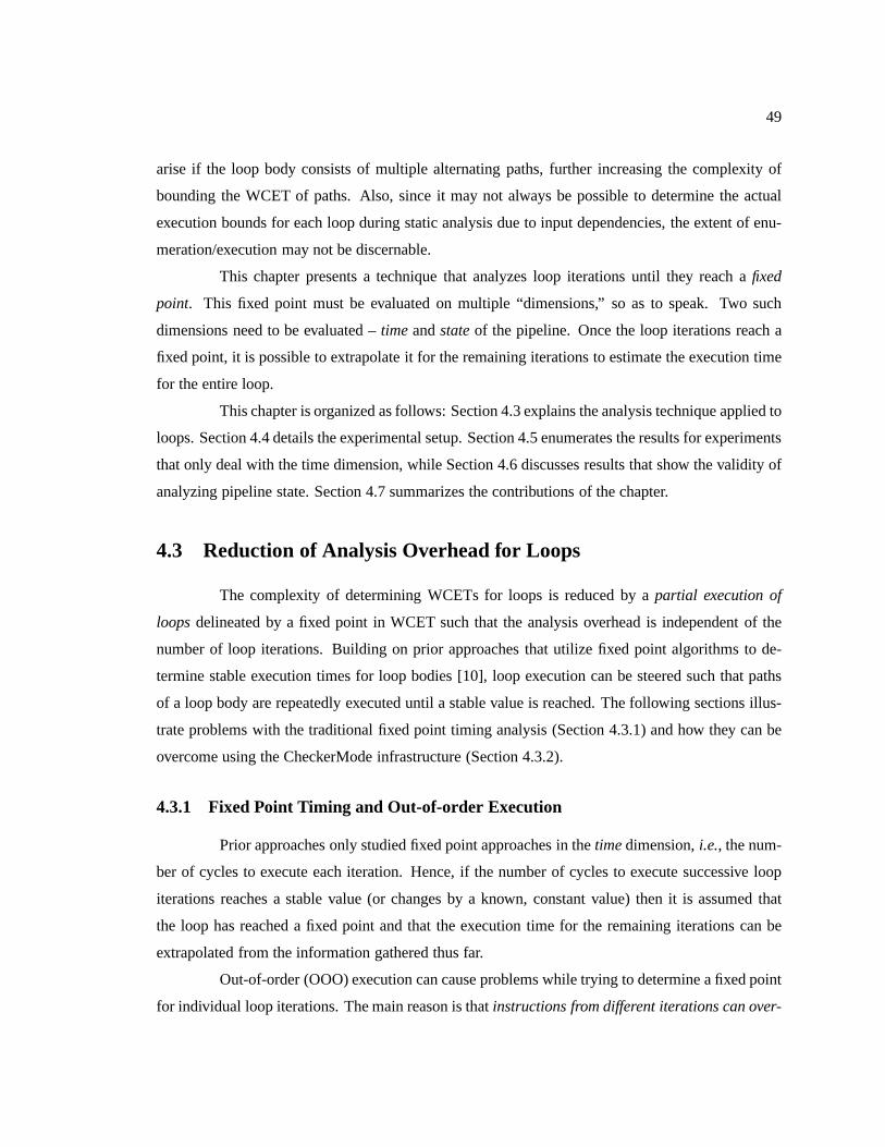
49

arise if the loop body consists of multiple alternating paths, further increasing the complexity of

bounding the WCET of paths. Also, since it may not always be possible to determine the actual

execution bounds for each loop during static analysis due toinput dependencies, the extent of enu-

meration/execution may not be discernable.

This chapter presents a technique that analyzes loop iterations until they reach afixed

point. This fixed point must be evaluated on multiple “dimensions,” so as to speak. Two such

dimensions need to be evaluated –timeandstateof the pipeline. Once the loop iterations reach a

fixed point, it is possible to extrapolate it for the remaining iterations to estimate the execution time

for the entire loop.

This chapter is organized as follows: Section 4.3 explains the analysis technique applied to

loops. Section 4.4 details the experimental setup. Section4.5 enumerates the results for experiments

that only deal with the time dimension, while Section 4.6 discusses results that show the validity of

analyzing pipeline state. Section 4.7 summarizes the contributions of the chapter.

4.3 Reduction of Analysis Overhead for Loops

The complexity of determining WCETs for loops is reduced by apartial execution of

loopsdelineated by a fixed point in WCET such that the analysis overhead is independent of the

number of loop iterations. Building on prior approaches that utilize fixed point algorithms to de-

termine stable execution times for loop bodies [10], loop execution can be steered such that paths

of a loop body are repeatedly executed until a stable value isreached. The following sections illus-

trate problems with the traditional fixed point timing analysis (Section 4.3.1) and how they can be

overcome using the CheckerMode infrastructure (Section 4.3.2).

4.3.1 Fixed Point Timing and Out-of-order Execution

Prior approaches only studied fixed point approaches in thetimedimension,i.e., the num-

ber of cycles to execute each iteration. Hence, if the numberof cycles to execute successive loop

iterations reaches a stable value (or changes by a known, constant value) then it is assumed that

the loop has reached a fixed point and that the execution time for the remaining iterations can be

extrapolated from the information gathered thus far.

Out-of-order (OOO) execution can cause problems while trying to determine a fixed point

for individual loop iterations. The main reason is thatinstructions from different iterations can over-

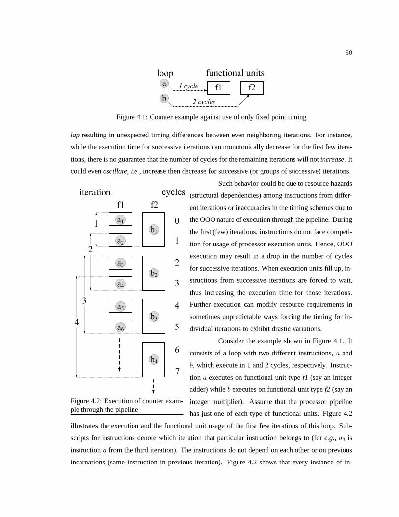
50

Figure 4.1: Counter example against use of only fixed point timing

lap resulting in unexpected timing differences between even neighboring iterations. For instance,

while the execution time for successive iterations can monotonically decrease for the first few itera-

tions, there is no guarantee that the number of cycles for theremaining iterations will notincrease. It

could evenoscillate, i.e., increase then decrease for successive (or groups of successive) iterations.

Figure 4.2: Execution of counter exam-ple through the pipeline

Such behavior could be due to resource hazards

(structural dependencies) among instructions from differ-

ent iterations or inaccuracies in the timing schemes due to

the OOO nature of execution through the pipeline. During

the first (few) iterations, instructions do not face competi-

tion for usage of processor execution units. Hence, OOO

execution may result in a drop in the number of cycles

for successive iterations. When execution units fill up, in-

structions from successive iterations are forced to wait,

thus increasing the execution time for those iterations.

Further execution can modify resource requirements in

sometimes unpredictable ways forcing the timing for in-

dividual iterations to exhibit drastic variations.

Consider the example shown in Figure 4.1. It

consists of a loop with two different instructions,a and

b, which execute in1 and2 cycles, respectively. Instruc-

tion a executes on functional unit typef1 (say an integer

adder) whileb executes on functional unit typef2 (say an

integer multiplier). Assume that the processor pipeline

has just one of each type of functional units. Figure 4.2

illustrates the execution and the functional unit usage of the first few iterations of this loop. Sub-

scripts for instructions denote which iteration that particular instruction belongs to (fore.g., a3 is

instructiona from the third iteration). The instructions do not depend oneach other or on previous

incarnations (same instruction in previous iteration). Figure 4.2 shows that every instance of in-

51

structionb executes in parallel withtwo instructions of typea. This is due to the fact that instruction

a takes only1 cycle to execute, and out of order instruction issue allows an instruction (a in this

case) from a future iteration to execute before instructionb completes. Hence, whilea1 andb1 start

at the same time (cycle0), a1 completes execution in1 cycle, thus freeing up functional unit f1.

Instructiona2 is issued to f1 even thoughb1 is not complete. Instructionsb1 anda2 complete at

the same time and vacate their respective functional units,at which time instructionsa3 andb2 are

issued.

Consider groups of instructions as successive iterations,as depicted on the left hand side

of Figure 4.2. Instructionsa1 andb1 constitute iteration1, instructionsa2 andb2 constitute iteration

2, etc.Let us make a simplifying assumption that each instruction takes the same number of cycles,

tB (representingtBefore), in the pipeline before reaching the issue/execute stage and also that each

instruction takes the same number of cycles,tA (representingtAfter), to exit from the pipeline once

it exits from its respective functional unit. LetcE (cEnter) represent the cycle when an instruction

enters its particular functional unit (i.e., its issue time) andce (cexit) represent the time when it

completed execution (i.e., it released the functional unit). Hence, using the “Path-Aggregate” timing

scheme described in from Section 2.4 (start timing apathwhen the first instruction from it is fetched

and stop when the last instruction retires), the execution time for loop iterationi will be:

ti = tBai+ (ce

bi− cE

ai) + tAbi

(4.1)

The middle term from Equation 4.1,(cebi−cE

ai), now denotes thepotential for variabilityin

execution time of each loop iteration during the execute stage. Substituting values from the example

in Figure 4.2, the respective execution times for iterations 1, 2, 3 and4 are:

t1 = tBa1+ 2 + tAb1

t2 = tBa2+ 3 + tAb2

t3 = tBa3+ 4 + tAb3

t4 = tBa4+ 5 + tAb4 (4.2)

Hence, the number of cycles calculated using traditional techniques can actually show anincrease

for successive loop iterations (for this particular example). This is an example of a loop where it is

difficult, if not impossible, to determine the fixed point forthe timing of individual loop iterations.

52

4.3.2 Fixed point Pipeline State Analysis using Reservation Stations

To tackle the problems due to OOO execution (Section 4.3.1),the fixed point analysis

technique is enhanced to findstable values in multiple “dimensions”(two, to be exact, for the given

constraints of only pipeline analysis in this dissertation):

1. time: the number of cycles to execute successive iterations through the pipeline must mono-

tonically decrease; and

2. pipeline state: the instructions in the reservation stations must repeat across groups of itera-

tions where a “group” is defined asone or moreiterations.

A controller records the monotonically decreasing execution times for each iteration up

to the fixed point using the CheckerMode hardware. The mechanism created to capture snapshots

(Chapter 3) is utilized to record the state of the reservation stations at the end of each iteration. The

example in Section 4.3.1 shows that just relying on the number of cycles to reach a fixed point may

not result in accurate timing values. In fact, it might not even be possible to detect a fixed point using

this approach. The state of reservation stations at the end of each iteration needs to be examined

across loop iterations (either with immediate neighbors, or over longer distances) tofind repeating

patternsof demands on the usage of execution units within the pipeline. E.g., if the snapshots (at the

end of each iteration) indicate that theexactsame instructions are using the same functional units

in successive iterations, then it can concluded that the execution of the loop through the pipeline

has reached a stable state.Note: It might be necessary to examine multiple loop iterations (perhaps

taken as groups) to find a repetitive pattern.

Hence, a search needs to be carried out on the state of the reservation stations such that

after iterationi, a pattern exists between iterationsi − x andi − y that is the same as the pattern

between iterationsk − x andk − y, wherek < i andx < y. Once such a pattern is found and the

execution times across those iterations are also seen to repeat, then the WCET for the remainder of

loop iterations, up to the loop bound, is calculated by a closed formula based on the fixed point value.

Figure 4.2 shows such a pattern repeating in loop iterationsthat are immediate neighbors. At the end

of each iteration,two instructions of type a andoneinstruction of type b have executed through the

functional units. This pattern repeats for all succeeding iterations. Even if the execution times do not

reach a fixed point value (example in Section 4.3.1), it mightbe possible to obtaincorrectandtight

fixed point values for loop iterations by examining the (stable) pipeline state. While Equation 4.2

shows that themeasuredexecution times for successive loop iterations increase, it might be possible

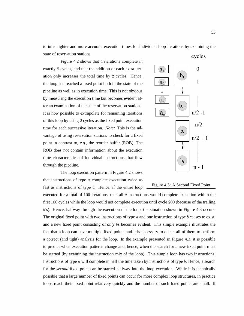
53

to infer tighter and more accurate execution times for individual loop iterations by examining the

state of reservation stations.

Figure 4.3: A Second Fixed Point

Figure 4.2 shows that4 iterations complete in

exactly8 cycles, and that the addition of each extra iter-

ation only increases the total time by2 cycles. Hence,

the loop has reached a fixed point both in the state of the

pipeline as well as in execution time. This is not obvious

by measuring the execution time but becomes evident af-

ter an examination of the state of the reservation stations.

It is now possible to extrapolate for remaining iterations

of this loop by using2 cycles as the fixed point execution

time for each successive iteration.Note: This is the ad-

vantage of using reservation stations to check for a fixed

point in contrast to,e.g., the reorder buffer (ROB). The

ROB does not contain information about the execution

time characteristics of individual instructions that flow

through the pipeline.

The loop execution pattern in Figure 4.2 shows

that instructions of typea complete execution twice as

fast as instructions of typeb. Hence, if the entire loop

executed for a total of100 iterations, then alla instructions would complete execution within the

first 100 cycles while the loop would not complete execution until cycle 200 (because of the trailing

b’s). Hence, halfway through the execution of the loop, the situation shown in Figure 4.3 occurs.

The original fixed point with two instructions of typea and one instruction of typeb ceases to exist,

and a new fixed point consisting ofonly bs becomes evident. This simple example illustrates the

fact that a loop can have multiple fixed points and it is necessary to detect all of them to perform

a correct (and tight) analysis for the loop. In the example presented in Figure 4.3, it is possible

to predict when execution patterns change and, hence, when the search for a new fixed point must

be started (by examining the instruction mix of the loop). This simple loop has two instructions.

Instructions of typea will complete in half the time taken by instructions of typeb. Hence, a search

for the secondfixed point can be started halfway into the loop execution. While it is technically

possible that a large number of fixed points can occur for morecomplex loop structures, in practice

loops reach their fixed point relatively quickly and the number of such fixed points are small. If

54

the total number of loops iterations is statically known, then it is possible to predict subsequent

fixed pointspreciselyand then use that information to estimate the correct WCET for the entire

loop. If the upper bound on loop iterations is not know, then the formulae calculating the worst-

case behavior of the loop can reflect a generic estimation on the locations of these fixed point (e.g.,

starting from cyclen/2 in Figure 4.3).

Figure 4.4: Alternative Execution Sce-nario for counter example

In the next example, if we relax the restrictive

assumption that the two functional units f1 and f2 (Fig-

ure 4.1) are different, then the execution pattern changes

to that shown in Figure 4.4. Since either instruction can

now execute on both functional units, instructionb2 gets

issued over instructiona3 at cycle number2 becauseb2

was fetched beforea3. Instructionsa3 anda4 are issued

in parallel with b2, but on functional unit f2. In cycle

4, both f1 and f2 execute instructions of typeb (b3 and

b4), since they are ahead of instructionsa5 anda6 in the

issue queue. Figure 4.4 shows that the pattern set in it-

erations1–4 (cycles0 to 5) repeats starting from cycle6.

Hence, to find a fixed point, analysis must be carried out

on consecutivegroupsof four iterations each. To calcu-

late the equivalent fixed point in time, the figure shows

that a group of4 iterations complete execution in6 cy-

cles. This can be used to extrapolate the WCET for the

remaining iterations.

Since the work in this dissertation only deals

with the analysis of the processor pipeline and related

effects, it is necessary to only analyzetwo dimensions

for evaluating the fixed point. In theory, similar analy-

sis could be extended to amulti-dimensionalfixed point

analysis, with additional “dimensions” representing other

processor features (e.g., branch predictors, caches).

Experimental results in Section 4.5 indicate that

loops reach a fixed point in the time dimension after only

3 iterations to account for pipeline effects. Another two iterations are required on average in the

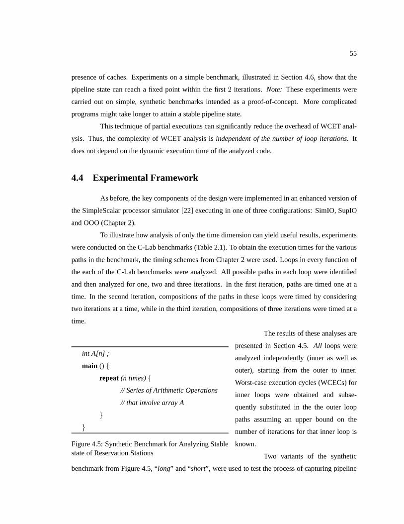
55

presence of caches. Experiments on a simple benchmark, illustrated in Section 4.6, show that the

pipeline state can reach a fixed point within the first2 iterations. Note: These experiments were

carried out on simple, synthetic benchmarks intended as a proof-of-concept. More complicated

programs might take longer to attain a stable pipeline state.

This technique of partial executions can significantly reduce the overhead of WCET anal-

ysis. Thus, the complexity of WCET analysis isindependent of the number of loop iterations. It

does not depend on the dynamic execution time of the analyzedcode.

4.4 Experimental Framework

As before, the key components of the design were implementedin an enhanced version of

the SimpleScalar processor simulator [22] executing in oneof three configurations: SimIO, SupIO

and OOO (Chapter 2).

To illustrate how analysis of only the time dimension can yield useful results, experiments

were conducted on the C-Lab benchmarks (Table 2.1). To obtain the execution times for the various

paths in the benchmark, the timing schemes from Chapter 2 were used. Loops in every function of

the each of the C-Lab benchmarks were analyzed. All possiblepaths in each loop were identified

and then analyzed for one, two and three iterations. In the first iteration, paths are timed one at a

time. In the second iteration, compositions of the paths in these loops were timed by considering

two iterations at a time, while in the third iteration, compositions of three iterations were timed at a

time.

int A[n] ;

main () {

repeat (n times){

// Series of Arithmetic Operations

// that involve array A

}

}

Figure 4.5: Synthetic Benchmark for Analyzing Stablestate of Reservation Stations

The results of these analyses are

presented in Section 4.5.All loops were

analyzed independently (inner as well as

outer), starting from the outer to inner.

Worst-case execution cycles (WCECs) for

inner loops were obtained and subse-

quently substituted in the the outer loop

paths assuming an upper bound on the

number of iterations for that inner loop is

known.

Two variants of the synthetic

benchmark from Figure 4.5, “long” and “short”, were used to test the process of capturing pipeline

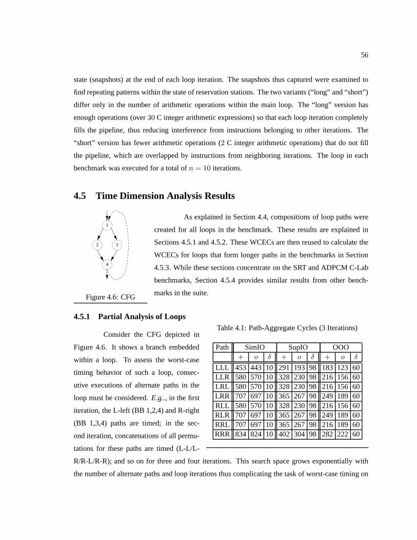
56

state (snapshots) at the end of each loop iteration. The snapshots thus captured were examined to

find repeating patterns within the state of reservation stations. The two variants (“long” and “short”)

differ only in the number of arithmetic operations within the main loop. The “long” version has

enough operations (over30 C integer arithmetic expressions) so that each loop iteration completely

fills the pipeline, thus reducing interference from instructions belonging to other iterations. The

“short” version has fewer arithmetic operations (2 C integer arithmetic operations) that do not fill

the pipeline, which are overlapped by instructions from neighboring iterations. The loop in each

benchmark was executed for a total ofn = 10 iterations.

4.5 Time Dimension Analysis Results

1

2 3

4

Figure 4.6: CFG

As explained in Section 4.4, compositions of loop paths were

created for all loops in the benchmark. These results are explained in

Sections 4.5.1 and 4.5.2. These WCECs are then reused to calculate the

WCECs for loops that form longer paths in the benchmarks in Section

4.5.3. While these sections concentrate on the SRT and ADPCMC-Lab

benchmarks, Section 4.5.4 provides similar results from other bench-

marks in the suite.

4.5.1 Partial Analysis of LoopsTable 4.1: Path-Aggregate Cycles (3 Iterations)

Path SimIO SupIO OOO+ o δ + o δ + o δ

LLL 453 443 10 291 193 98 183 123 60LLR 580 570 10 328 230 98 216 156 60LRL 580 570 10 328 230 98 216 156 60LRR 707 697 10 365 267 98 249 189 60RLL 580 570 10 328 230 98 216 156 60RLR 707 697 10 365 267 98 249 189 60RRL 707 697 10 365 267 98 216 189 60RRR 834 824 10 402 304 98 282 222 60

Consider the CFG depicted in

Figure 4.6. It shows a branch embedded

within a loop. To assess the worst-case

timing behavior of such a loop, consec-

utive executions of alternate paths in the

loop must be considered.E.g.., in the first

iteration, the L-left (BB 1,2,4) and R-right

(BB 1,3,4) paths are timed; in the sec-

ond iteration, concatenations of all permu-

tations for these paths are timed (L-L/L-

R/R-L/R-R); and so on for three and four iterations. This search space grows exponentially with

the number of alternate paths and loop iterations thus complicating the task of worst-case timing on

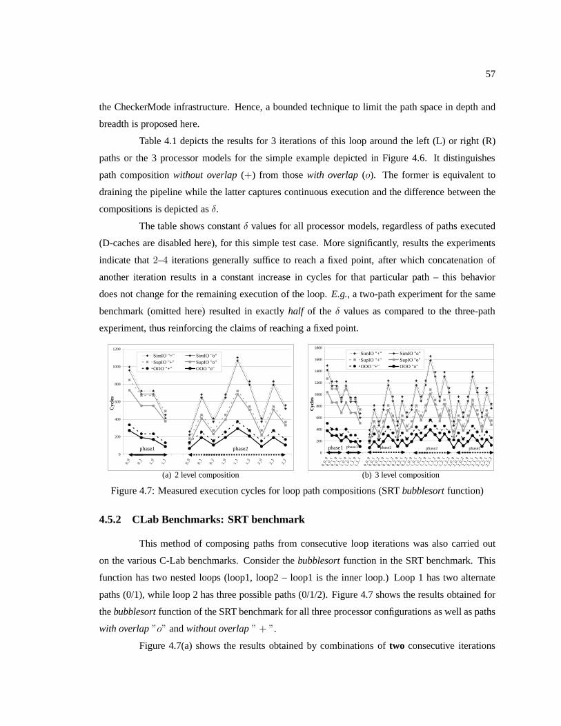
57

the CheckerMode infrastructure. Hence, a bounded technique to limit the path space in depth and

breadth is proposed here.

Table 4.1 depicts the results for 3 iterations of this loop around the left (L) or right (R)

paths or the 3 processor models for the simple example depicted in Figure 4.6. It distinguishes

path compositionwithout overlap(+) from thosewith overlap (o). The former is equivalent to

draining the pipeline while the latter captures continuousexecution and the difference between the

compositions is depicted asδ.

The table shows constantδ values for all processor models, regardless of paths executed

(D-caches are disabled here), for this simple test case. More significantly, results the experiments

indicate that2–4 iterations generally suffice to reach a fixed point, after which concatenation of

another iteration results in a constant increase in cycles for that particular path – this behavior

does not change for the remaining execution of the loop.E.g., a two-path experiment for the same

benchmark (omitted here) resulted in exactlyhalf of the δ values as compared to the three-path

experiment, thus reinforcing the claims of reaching a fixed point.

0

200

400

600

800

1000

1200

0_0

0_1

1_0

1_1

0_0

0_1

0_2

1_0

1_1

1_2

2_0

2_1

2_2

Cyc

les

SimIO "+" SimIO "o"SupIO "+" SupIO "o"OOO "+" OOO "o"

phase1 phase2

(a) 2 level composition

0

200

400

600

800

1000

1200

1400

1600

1800

0_0_

00_

0_1

0_1_

00_

1_1

1_0_

01_

0_1

1_1_

01_

1_1

0_0_

00_

0_1

0_0_

20_

1_0

0_1_

10_

1_2

0_2_

00_

2_1

0_2_

21_

0_0

1_0_

11_

0_2

1_1_

01_

1_1

1_1_

21_

2_0

1_2_

11_

2_2

2_0_

02_

0_1

2_0_

22_

1_0

2_1_

12_

1_2

2_2_

02_

2_1

2_2_

2

Cyc

les

SimIO "+" SimIO "o"SupIO "+" SupIO "o"OOO "+" OOO "o"

phase1phase1 phase2 phase2 phase2

(b) 3 level composition

Figure 4.7: Measured execution cycles for loop path compositions (SRTbubblesortfunction)

4.5.2 CLab Benchmarks: SRT benchmark

This method of composing paths from consecutive loop iterations was also carried out

on the various C-Lab benchmarks. Consider thebubblesortfunction in the SRT benchmark. This

function has two nested loops (loop1, loop2 – loop1 is the inner loop.) Loop 1 has two alternate

paths (0/1), while loop 2 has three possible paths (0/1/2). Figure 4.7 shows the results obtained for

thebubblesortfunction of the SRT benchmark for all three processor configurations as well as paths

with overlap”o” andwithout overlap” + ”.

Figure 4.7(a) shows the results obtained by combinations oftwo consecutive iterations

58

at a time and Figure 4.7(b) shows similar results for combinations of three consecutive iterations

at a time. The x-axis labels in Figure 4.7 refer to path concatenations, i.e., 0 1 2 refers to the

concatenated execution of paths0, 1 and2. Theydo notrefer to loops. The two separate plots in

each graph demarcate results for each loop.

Table 4.2: Path-Aggregate Cycles (2 Iterations) for the bub-blesort function of SRT.

Id Path SimIO SupIO OOO+ o δ + o δ + o δ

1 0 0 996 958 38 848 731 117 336 272 641 0 1 723 685 38 671 554 117 234 189 451 1 0 723 685 38 671 554 117 234 170 641 1 1 450 412 38 494 377 117 132 87 45

2 0 0 260 222 38 180 120 60 134 67 672 0 1 682 645 37 451 409 42 254 189 652 0 2 409 372 37 274 232 42 152 106 462 1 0 682 645 37 451 396 55 254 191 632 1 1 1104 1066 38 722 685 37 374 291 832 1 2 831 793 38 545 508 37 272 208 642 2 0 409 372 37 274 219 55 152 89 632 2 1 831 793 38 545 508 37 272 189 83

At the outset, it can be

seen that all path compositions fol-

low the strict ordering ofSimIO ≥

SupIO ≥ OOO. Also note that

the execution of the three-level com-

positions exceed those of the two-

level compositions by a uniform con-

stant. This is immediately obvious

while comparing the regions marked

asphasesin both graphs. For Loop

1 (phase 1) the “shape” of the graph

from Figure 4.7(a) is repeated in Fig-

ure 4.7(b). The difference is that the

actual execution cycles are higher (by

this uniform constant) for the three-

path compositions.

Hence, increasing the level of compositions increases the execution time by a constant

value for each path composition. Similar results are evident for the more complicated outer loop

(loop 2) with three alternate paths (0/1/2). The shape of ”phase 2” repeats multiple times in the three-

way composition, thus indicating that the execution cyclesfor the these paths are offset by a constant

from corresponding two-way path compositions. Thus, any further increases in composition depth

will only add a constant value to the path execution time. Hence, a fixed point has been reached for

the loops inthreeiterations.

It is also interesting to note that while the actual permutation of paths are not necessarily

related to each other, their relative order in the plot showsan important result – that increasing

loop composition “depth” increased the cost of execution for that path by a uniform constant value,

(illustrated by the shape of the graph).

It can be seen that the paths have reached a fixed point from thedifferences between path

compositionswithout overlapandwith overlapin Tables 4.2 and 4.3. The former (without overlap)

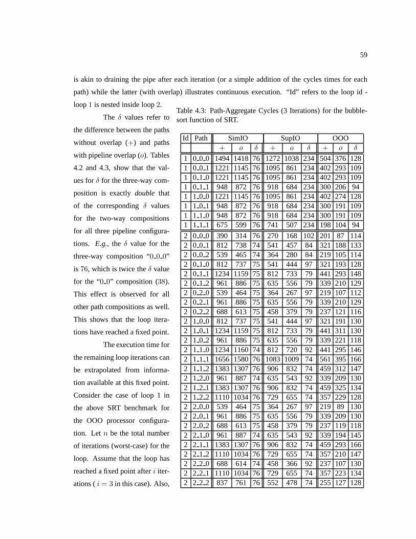
59

is akin to draining the pipe after each iteration (or a simpleaddition of the cycles times for each

path) while the latter (with overlap) illustrates continuous execution. “Id” refers to the loop id -

loop1 is nested inside loop2.Table 4.3: Path-Aggregate Cycles (3 Iterations) for the bubble-sort function of SRT.

Id Path SimIO SupIO OOO+ o δ + o δ + o δ

1 0 0 0 1494 1418 76 1272 1038 234 504 376 1281 0 0 1 1221 1145 76 1095 861 234 402 293 1091 0 1 0 1221 1145 76 1095 861 234 402 293 1091 0 1 1 948 872 76 918 684 234 300 206 941 1 0 0 1221 1145 76 1095 861 234 402 274 1281 1 0 1 948 872 76 918 684 234 300 191 1091 1 1 0 948 872 76 918 684 234 300 191 1091 1 1 1 675 599 76 741 507 234 198 104 94

2 0 0 0 390 314 76 270 168 102 201 87 1142 0 0 1 812 738 74 541 457 84 321 188 1332 0 0 2 539 465 74 364 280 84 219 105 1142 0 1 0 812 737 75 541 444 97 321 193 1282 0 1 1 1234 1159 75 812 733 79 441 293 1482 0 1 2 961 886 75 635 556 79 339 210 1292 0 2 0 539 464 75 364 267 97 219 107 1122 0 2 1 961 886 75 635 556 79 339 210 1292 0 2 2 688 613 75 458 379 79 237 121 1162 1 0 0 812 737 75 541 444 97 321 191 1302 1 0 1 1234 1159 75 812 733 79 441 311 1302 1 0 2 961 886 75 635 556 79 339 221 1182 1 1 0 1234 1160 74 812 720 92 441 295 1462 1 1 1 1656 1580 76 1083 1009 74 561 395 1662 1 1 2 1383 1307 76 906 832 74 459 312 1472 1 2 0 961 887 74 635 543 92 339 209 1302 1 2 1 1383 1307 76 906 832 74 459 325 1342 1 2 2 1110 1034 76 729 655 74 357 229 1282 2 0 0 539 464 75 364 267 97 219 89 1302 2 0 1 961 886 75 635 556 79 339 209 1302 2 0 2 688 613 75 458 379 79 237 119 1182 2 1 0 961 887 74 635 543 92 339 194 1452 2 1 1 1383 1307 76 906 832 74 459 293 1662 2 1 2 1110 1034 76 729 655 74 357 210 1472 2 2 0 688 614 74 458 366 92 237 107 1302 2 2 1 1110 1034 76 729 655 74 357 223 1342 2 2 2 837 761 76 552 478 74 255 127 128

The δ values refer to

the difference between the paths

without overlap (+) and paths

with pipeline overlap (o). Tables

4.2 and 4.3, show that the val-

ues forδ for the three-way com-

position is exactlydouble that

of the correspondingδ values

for the two-way compositions

for all three pipeline configura-

tions. E.g., the δ value for the

three-way composition “0 0 0”

is 76, which is twice theδ value

for the “0 0” composition (38).

This effect is observed for all

other path compositions as well.

This shows that the loop itera-

tions have reached a fixed point.

The execution time for

the remaining loop iterations can

be extrapolated from informa-

tion available at this fixed point.

Consider the case of loop 1 in

the above SRT benchmark for

the OOO processor configura-

tion. Let n be the total number

of iterations (worst-case) for the

loop. Assume that the loop has

reached a fixed point afteri iter-

ations (i = 3 in this case). Also,

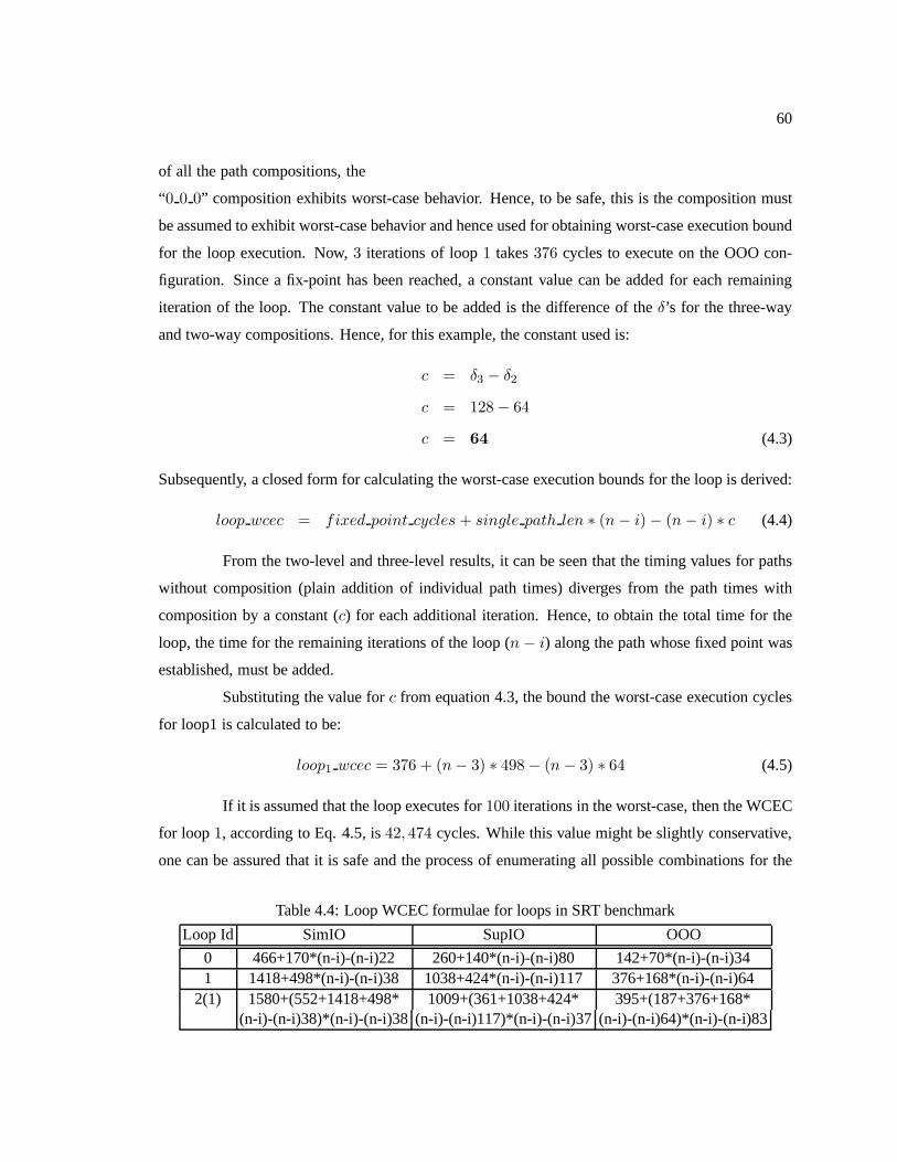
60

of all the path compositions, the

“0 0 0” composition exhibits worst-case behavior. Hence, to be safe, this is the composition must

be assumed to exhibit worst-case behavior and hence used forobtaining worst-case execution bound

for the loop execution. Now,3 iterations of loop1 takes376 cycles to execute on the OOO con-

figuration. Since a fix-point has been reached, a constant value can be added for each remaining

iteration of the loop. The constant value to be added is the difference of theδ’s for the three-way

and two-way compositions. Hence, for this example, the constant used is:

c = δ3 − δ2

c = 128− 64

c = 64 (4.3)

Subsequently, a closed form for calculating the worst-caseexecution bounds for the loop is derived:

loop wcec = fixed point cycles + single path len ∗ (n− i)− (n− i) ∗ c (4.4)

From the two-level and three-level results, it can be seen that the timing values for paths

without composition (plain addition of individual path times) diverges from the path times with

composition by a constant (c) for each additional iteration. Hence, to obtain the total time for the

loop, the time for the remaining iterations of the loop (n − i) along the path whose fixed point was

established, must be added.

Substituting the value forc from equation 4.3, the bound the worst-case execution cycles

for loop1 is calculated to be:

loop1 wcec = 376 + (n− 3) ∗ 498− (n− 3) ∗ 64 (4.5)

If it is assumed that the loop executes for100 iterations in the worst-case, then the WCEC

for loop 1, according to Eq. 4.5, is42, 474 cycles. While this value might be slightly conservative,

one can be assured that it is safe and the process of enumerating all possible combinations for the

Table 4.4: Loop WCEC formulae for loops in SRT benchmark

Loop Id SimIO SupIO OOO

0 466+170*(n-i)-(n-i)22 260+140*(n-i)-(n-i)80 142+70*(n-i)-(n-i)341 1418+498*(n-i)-(n-i)38 1038+424*(n-i)-(n-i)117 376+168*(n-i)-(n-i)64

2(1) 1580+(552+1418+498* 1009+(361+1038+424* 395+(187+376+168*(n-i)-(n-i)38)*(n-i)-(n-i)38 (n-i)-(n-i)117)*(n-i)-(n-i)37 (n-i)-(n-i)64)*(n-i)-(n-i)83

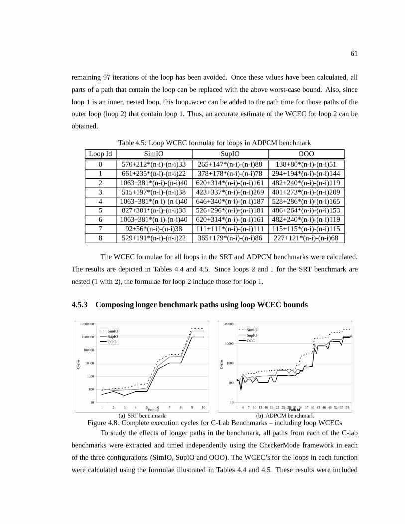
61

remaining97 iterations of the loop has been avoided. Once these values have been calculated, all

parts of a path that contain the loop can be replaced with the above worst-case bound. Also, since

loop 1 is an inner, nested loop, this loopwcec can be added to the path time for those paths of the

outer loop (loop 2) that contain loop 1. Thus, an accurate estimate of the WCEC for loop 2 can be

obtained.

Table 4.5: Loop WCEC formulae for loops in ADPCM benchmark

Loop Id SimIO SupIO OOO

0 570+212*(n-i)-(n-i)33 265+147*(n-i)-(n-i)88 138+80*(n-i)-(n-i)511 661+235*(n-i)-(n-i)22 378+178*(n-i)-(n-i)78 294+194*(n-i)-(n-i)1442 1063+381*(n-i)-(n-i)40 620+314*(n-i)-(n-i)161 482+240*(n-i)-(n-i)1193 515+197*(n-i)-(n-i)38 423+337*(n-i)-(n-i)269 401+273*(n-i)-(n-i)2094 1063+381*(n-i)-(n-i)40 646+340*(n-i)-(n-i)187 528+286*(n-i)-(n-i)1655 827+301*(n-i)-(n-i)38 526+296*(n-i)-(n-i)181 486+264*(n-i)-(n-i)1536 1063+381*(n-i)-(n-i)40 620+314*(n-i)-(n-i)161 482+240*(n-i)-(n-i)1197 92+56*(n-i)-(n-i)38 111+111*(n-i)-(n-i)111 115+115*(n-i)-(n-i)1158 529+191*(n-i)-(n-i)22 365+179*(n-i)-(n-i)86 227+121*(n-i)-(n-i)68

The WCEC formulae for all loops in the SRT and ADPCM benchmarks were calculated.

The results are depicted in Tables 4.4 and 4.5. Since loops2 and1 for the SRT benchmark are

nested (1 with 2), the formulae for loop2 include those for loop1.

4.5.3 Composing longer benchmark paths using loop WCEC bounds

10

100

1000

10000

100000

1000000

10000000

1 2 3 4 5 6 7 8 9 10Path Id

Cyc

les

SimIOSupIOOOO

(a) SRT benchmark

10

100

1000

10000

100000

1 4 7 10 13 16 19 22 25 28 31 34 37 40 43 46 49 52 55 58Path Id

Cyc

les

SimIOSupIOOOO

(b) ADPCM benchmarkFigure 4.8: Complete execution cycles for C-Lab Benchmarks– including loop WCECs

To study the effects of longer paths in the benchmark, all paths from each of the C-lab

benchmarks were extracted and timed independently using the CheckerMode framework in each

of the three configurations (SimIO, SupIO and OOO). The WCEC’s for the loops in each function

were calculated using the formulae illustrated in Tables 4.4 and 4.5. These results were included

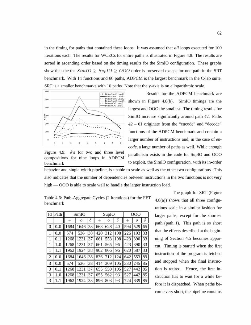
62

in the timing for paths that contained these loops. It was assumed thatall loops executed for100

iterations each. The results for WCECs for entire paths is illustrated in Figure 4.8. The results are

sorted in ascending order based on the timing results for theSimIO configuration. These graphs

show that the theSimIO ≥ SupIO ≥ OOO order is preserved except for one path in the SRT

benchmark. With14 functions and60 paths, ADPCM is the largest benchmark in the C-lab suite.

SRT is a smaller benchmarks with10 paths. Note that the y-axis is on a logarithmic scale.

0

100

200

300

400

500

600

0 1 2 3 4 5 6 7 8

Cyc

les

Deltas SimIO Level 2Deltas SimIO Level 3Deltas SupIO Level 2Deltas SupIO Level 3Deltas OOO Level 2Deltas OOO Level 3

Figure 4.9: δ’s for two and three levelcompositions for nine loops in ADPCMbenchmark

Results for the ADPCM benchmark are

shown in Figure 4.8(b). SimIO timings are the

largest and OOO the smallest. The timing results for

SimIO increase significantly around path42. Paths

42 – 61 originate from the “encode” and “decode”

functions of the ADPCM benchmark and contain a

larger number of instructions and, in the case ofen-

code, a large number of paths as well. While enough

parallelism exists in the code for SupIO and OOO

to exploit, the SimIO configuration, with its in-order

behavior and single width pipeline, is unable to scale as well as the other two configurations. This

also indicates that the number of dependencies between instructions in the two functions is not very

high — OOO is able to scale well to handle the larger instruction load.

Table 4.6: Path-Aggregate Cycles (2 Iterations) for the FFTbenchmark

Id Path SimIO SupIO OOO+ o δ + o δ + o δ

0 0 0 1684 1646 38 668 628 40 594 529 65

1 0 0 574 536 38 420 312 108 226 193 331 0 1 1268 1231 37 661 553 108 423 390 331 1 0 1268 1231 37 661 565 96 423 390 331 1 1 1962 1924 38 902 806 96 620 587 33

2 0 0 1684 1646 38 836 712 124 642 553 89

3 0 0 574 536 38 414 309 105 330 245 853 0 1 1268 1231 37 655 550 105 527 442 853 1 0 1268 1231 37 655 562 93 527 442 853 1 1 1962 1924 38 896 803 93 724 639 85

The graph for SRT (Figure

4.8(a)) shows that all three configu-

rations scale in a similar fashion for

larger paths, except for the shortest

path (path 1). This path is so short

that the effects described at the begin-

ning of Section 4.5 becomes appar-

ent. Timing is started when the first

instruction of the program is fetched

and stopped when the final instruc-

tion is retired. Hence, the first in-

struction has to wait for a while be-

fore it is dispatched. When paths be-

come very short, the pipeline contains

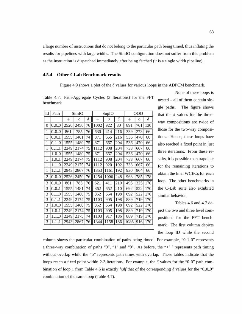
63

a large number of instructions that do not belong to the particular path being timed, thus inflating the

results for pipelines with large widths. The SimIO configuration does not suffer from this problem

as the instruction is dispatched immediately after being fetched (it is a single width pipeline).

4.5.4 Other CLab Benchmark results

Figure 4.9 shows a plot of theδ values for various loops in the ADPCM benchmark.

Table 4.7: Path-Aggregate Cycles (3 Iterations) for the FFTbenchmark

Id Path SimIO SupIO OOO+ o δ + o δ + o δ

0 0 0 0 2526 2450 76 1002 922 80 891 761 130

1 0 0 0 861 785 76 630 414 216 339 273 661 0 0 1 1555 1481 74 871 655 216 536 470 661 0 1 0 1555 1480 75 871 667 204 536 470 661 0 1 1 2249 2174 75 1112 908 204 733 667 661 1 0 0 1555 1480 75 871 667 204 536 470 661 1 0 1 2249 2174 75 1112 908 204 733 667 661 1 1 0 2249 2175 74 1112 920 192 733 667 661 1 1 1 2943 2867 76 1353 1161 192 930 864 66

2 0 0 0 2526 2450 76 1254 1006 248 963 785 178

3 0 0 0 861 785 76 621 411 210 495 325 1703 0 0 1 1555 1481 74 862 652 210 692 522 1703 0 1 0 1555 1480 75 862 664 198 692 522 1703 0 1 1 2249 2174 75 1103 905 198 889 719 1703 1 0 0 1555 1480 75 862 664 198 692 522 1703 1 0 1 2249 2174 75 1103 905 198 889 719 1703 1 1 0 2249 2175 74 1103 917 186 889 719 1703 1 1 1 2943 2867 76 1344 1158 186 1086 916 170

None of these loops is

nested – all of them contain sin-

gle paths. The figure shows

that theδ values for the three-

way compositions are twice of

those for the two-way composi-

tions. Hence, these loops have

also reached a fixed point in just

three iterations. From these re-

sults, it is possible to extrapolate

for the remaining iterations to

obtain the final WCECs for each

loop. The other benchmarks in

the C-Lab suite also exhibited

similar behavior.

Tables 4.6 and 4.7 de-

pict the two and three level com-

positions for the FFT bench-

mark. The first column depicts

the loop ID while the second

column shows the particular combination of paths being timed. For example, “01 0” represents

a three-way combination of paths “0”, “1” and “0”. As before,the “+’ ’ represents path timing

without overlap while the “o” represents path times with overlap. These tables indicate that the

loops reach a fixed point within 2-3 iterations. For example,the δ values for the “00” path com-

bination of loop 1 from Table 4.6 is exactlyhalf that of the correspondingδ values for the “00 0”

combination of the same loop (Table 4.7).

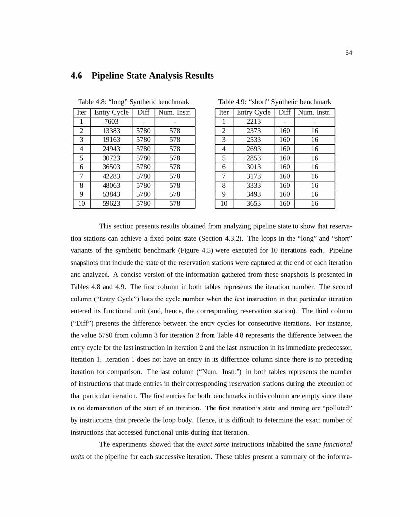
64

4.6 Pipeline State Analysis Results

Table 4.8: “long” Synthetic benchmark

Iter Entry Cycle Diff Num. Instr.1 7603 - -2 13383 5780 5783 19163 5780 5784 24943 5780 5785 30723 5780 5786 36503 5780 5787 42283 5780 5788 48063 5780 5789 53843 5780 57810 59623 5780 578

Table 4.9: “short” Synthetic benchmark

Iter Entry Cycle Diff Num. Instr.1 2213 - -2 2373 160 163 2533 160 164 2693 160 165 2853 160 166 3013 160 167 3173 160 168 3333 160 169 3493 160 1610 3653 160 16

This section presents results obtained from analyzing pipeline state to show that reserva-

tion stations can achieve a fixed point state (Section 4.3.2). The loops in the “long” and “short”

variants of the synthetic benchmark (Figure 4.5) were executed for 10 iterations each. Pipeline

snapshots that include the state of the reservation stations were captured at the end of each iteration

and analyzed. A concise version of the information gatheredfrom these snapshots is presented in

Tables 4.8 and 4.9. The first column in both tables representsthe iteration number. The second

column (“Entry Cycle”) lists the cycle number when thelast instruction in that particular iteration

entered its functional unit (and, hence, the correspondingreservation station). The third column

(“Diff”) presents the difference between the entry cycles for consecutive iterations. For instance,

the value5780 from column3 for iteration2 from Table 4.8 represents the difference between the

entry cycle for the last instruction in iteration2 and the last instruction in its immediate predecessor,

iteration1. Iteration1 does not have an entry in its difference column since there isno preceding

iteration for comparison. The last column (“Num. Instr.”) in both tables represents the number

of instructions that made entries in their corresponding reservation stations during the execution of

that particular iteration. The first entries for both benchmarks in this column are empty since there

is no demarcation of the start of an iteration. The first iteration’s state and timing are “polluted”

by instructions that precede the loop body. Hence, it is difficult to determine the exact number of

instructions that accessed functional units during that iteration.

The experiments showed that theexact sameinstructions inhabited thesame functional

unitsof the pipeline for each successive iteration. These tablespresent a summary of the informa-

65

tion obtained from studying the reservation station state captured after each iteration since it is not

feasible to present the list of all instructions in the reservation stations (578 of them in the long ver-

sion) for all iterations. An examination of the “Diff” column shows that the last instruction of each

iteration enters its functional unit a constant time step after its corresponding predecessor from the

previous iteration. This also reveals the fact that this benchmark has not only reached a fixed point

in the pipeline state but also in the time domain. This “Diff”value can be utilized to extrapolate the

WCET for the remaining iterations of the loop.

The last column shows that every iteration (except the first)has the exact same number

of instructions that access functional units (and make corresponding entries in their reservation

stations). In fact, a visual inspection of the snapshot state showed that the instructions (578 for

“long” and 16 for “short”) were identical across iterations. Hence, these benchmarks reached a

stable pipeline state in2 iterations. These results show that an examination of the pipeline state for

loop iterations can provide a more complete fixed point analysis.

4.7 Conclusion

The work outlined in this chapter provides the means to accurately bound the worst-case

execution time for a given program path using a combination of the traditional fixed point timing

analysis approach and an examination of the pipeline state from each iteration. The former consists

of a synergistic combination of analytical closed-formuladerivations and observed actual timings

of execution under the CheckerMode. The latter utilizes thesnapshot mechanism of CheckerMode

to capture the state of reservation stations (and, hence, the usage of functional units) after every

iteration and then attempts to find repeating patterns in that state.

This chapter develops and evaluates these techniques for loop and, ultimately, whole task

analysis to help derive bounds on the WCET. These techniquesprovide a mechanism to perform a

partial analysis for loops. This mechanism does not require a complete enumeration or execution

of all iterations in the loop. An interesting outcome of the analysis is the amount of architectural

state that must be closely followed for performing an accurate analysis. The retire stage and the

issue/execute stages must be captured to reflect the worst-case behavior of loop iterations in an

OOO pipeline.

66

Chapter 5

Parametric Timing Analysis and Its

Application to Dynamic Voltage Scaling

5.1 Summary

Static timing analysis derives bounds on worst-case execution times (WCETs) but requires

statically known loop bounds. This chapter describes work that removes this constraint on known

loop bounds through parametric analysis which expresses WCETs as functions. Tighter WCETs

are dynamically discovered to exploit slack by dynamic voltage scaling (DVS) saving 60%-82%

energy over DVS-oblivious techniques and showing savings close to more costly dynamic-priority

DVS algorithms.

Overall, parametric analysis expands the class of real-time applications to programs with

loop-invariant dynamic loop bounds while retaining tight WCET bounds.

5.2 Introduction

Static timing analysis provides bounds on the WCET but thesebounds require constraints

to be imposed on the tasks (timed code), the most striking of which is the requirement to statically

bound the number of iterations of loops within the task. These loop bounds address the halting

problem,i.e., without these loop bounds, WCET bounds cannot be derived. The programmer must

provide these upper bounds on loop iterations when they cannot be inferred by program analysis.

Hence, these statically fixed loop bounds may present an inconvenience. They also restrict the class

of programs that can be used in real-time systems. This type of timing analysis is referred to as

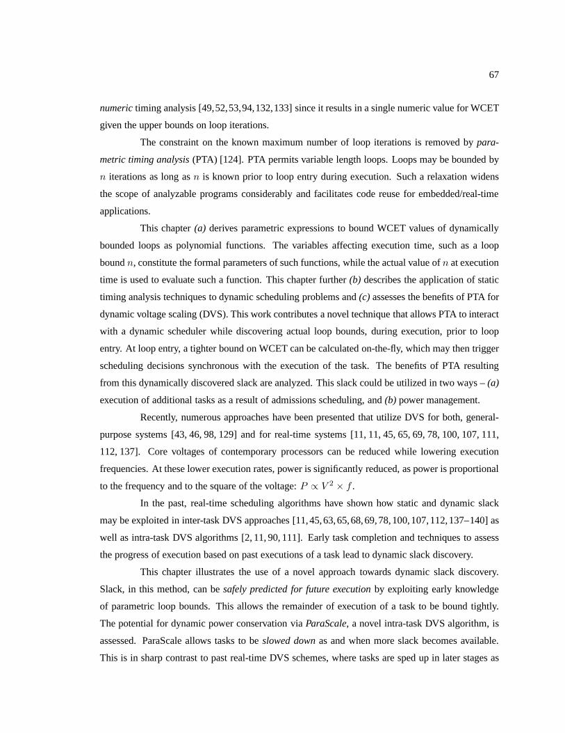
67

numerictiming analysis [49,52,53,94,132,133] since it results ina single numeric value for WCET

given the upper bounds on loop iterations.

The constraint on the known maximum number of loop iterations is removed bypara-

metric timing analysis(PTA) [124]. PTA permits variable length loops. Loops may bebounded by

n iterations as long asn is known prior to loop entry during execution. Such a relaxation widens

the scope of analyzable programs considerably and facilitates code reuse for embedded/real-time

applications.

This chapter(a) derives parametric expressions to bound WCET values of dynamically

bounded loops as polynomial functions. The variables affecting execution time, such as a loop

boundn, constitute the formal parameters of such functions, whilethe actual value ofn at execution

time is used to evaluate such a function. This chapter further (b) describes the application of static

timing analysis techniques to dynamic scheduling problemsand(c) assesses the benefits of PTA for

dynamic voltage scaling (DVS). This work contributes a novel technique that allows PTA to interact

with a dynamic scheduler while discovering actual loop bounds, during execution, prior to loop

entry. At loop entry, a tighter bound on WCET can be calculated on-the-fly, which may then trigger

scheduling decisions synchronous with the execution of thetask. The benefits of PTA resulting

from this dynamically discovered slack are analyzed. This slack could be utilized in two ways –(a)

execution of additional tasks as a result of admissions scheduling, and(b) power management.

Recently, numerous approaches have been presented that utilize DVS for both, general-

purpose systems [43, 46, 98, 129] and for real-time systems [11, 11, 45, 65, 69, 78, 100, 107, 111,

112, 137]. Core voltages of contemporary processors can be reduced while lowering execution

frequencies. At these lower execution rates, power is significantly reduced, as power is proportional

to the frequency and to the square of the voltage:P ∝ V 2 × f .

In the past, real-time scheduling algorithms have shown howstatic and dynamic slack

may be exploited in inter-task DVS approaches [11,45,63,65,68,69,78,100,107,112,137–140] as

well as intra-task DVS algorithms [2, 11, 90, 111]. Early task completion and techniques to assess

the progress of execution based on past executions of a task lead to dynamic slack discovery.

This chapter illustrates the use of a novel approach towardsdynamic slack discovery.

Slack, in this method, can besafely predicted for future executionby exploiting early knowledge

of parametric loop bounds. This allows the remainder of execution of a task to be bound tightly.

The potential for dynamic power conservation viaParaScale, a novel intra-task DVS algorithm, is

assessed. ParaScale allows tasks to beslowed downas and when more slack becomes available.

This is in sharp contrast to past real-time DVS schemes, where tasks are sped up in later stages as

68

they approach their deadline [45,63,68,138–140].

This chapter also describes a novel enhancement to the static DVS scheme which, incor-

porated with the intra-task slack determination scheme results in significant energy savings. The en-

ergy savings approach those obtained by one of the most aggressive dynamic DVS algorithms [100].

The approach is evaluated by implementing PTA in a gcc environment with a MIPS-like

instruction set. Execution is simulated on a customized SimpleScalar [21] framework that supports

multi-tasking. The effects of instruction cache misses arebounded in the experiments, but preclude

the effects of data cache misses. The framework has been modified to support customized schedulers

with and without DVS policies and an enhanced Wattch power model [20], which aids in assessing

power consumption. A more accurate leakage power model [64]was also implemented to estimate

the amount of leakage and static power consumed by the processor. This framework is used to study

the benefits of PTA in the context of ParaScale as a means to exploit DVS.

Results show that ParaScale, applied on a modified version ofa static DVS algorithm,

provides significant savings by utilizing the parametric approach to timing analysis. These savings

are observed for generated dynamic slack and potential reduction in overall energy. In fact, the

amount of energy saved is very close to that obtained by the lookahead EDF-DVS scheme [100] –

a popular, aggressivedynamicDVS algorithm. Thus, ParaScale makes it possible for staticinter-

task DVS algorithms to be used on embedded systems. This helps avoid more cumbersome (and

difficult to implement) DVS schemes while still achieving similar energy savings. The approach

presented here utilizes online intra-task DVS to exploit parametric execution times resulting in much

lower power consumptions,i.e., even without any scheduler-assisted DVS savings. Hence, even

in the absence of dynamic priority scheduling, significant power savings may be achieved,e.g.,

in the case of cyclic executives or fixed-priority policies such as rate-monotonic schedulers [76].

Overall, parametric timing analysis expands the class of applications for real-time systems to include

programs with dynamic loop bounds that are loop invariant while retaining tight WCET bounds and

uncovering additional slack in the schedule.

This chapter is structured as follows. Sections 5.3 and 5.4 provide information on nu-

meric and parametric timing analysis respectively. Section 5.5 explains derivation of the parametric

formulae and their integration into the code of tasks. This section also shows the steps involved in

obtaining accurate WCET analysis for the new, enhanced code. Section 5.6 discusses the context in

which parametric timing results are used. Section 5.7 introduces the simulation framework. Section

5.8 elaborates on the experiments and results. Section 5.9 summarizes the work.

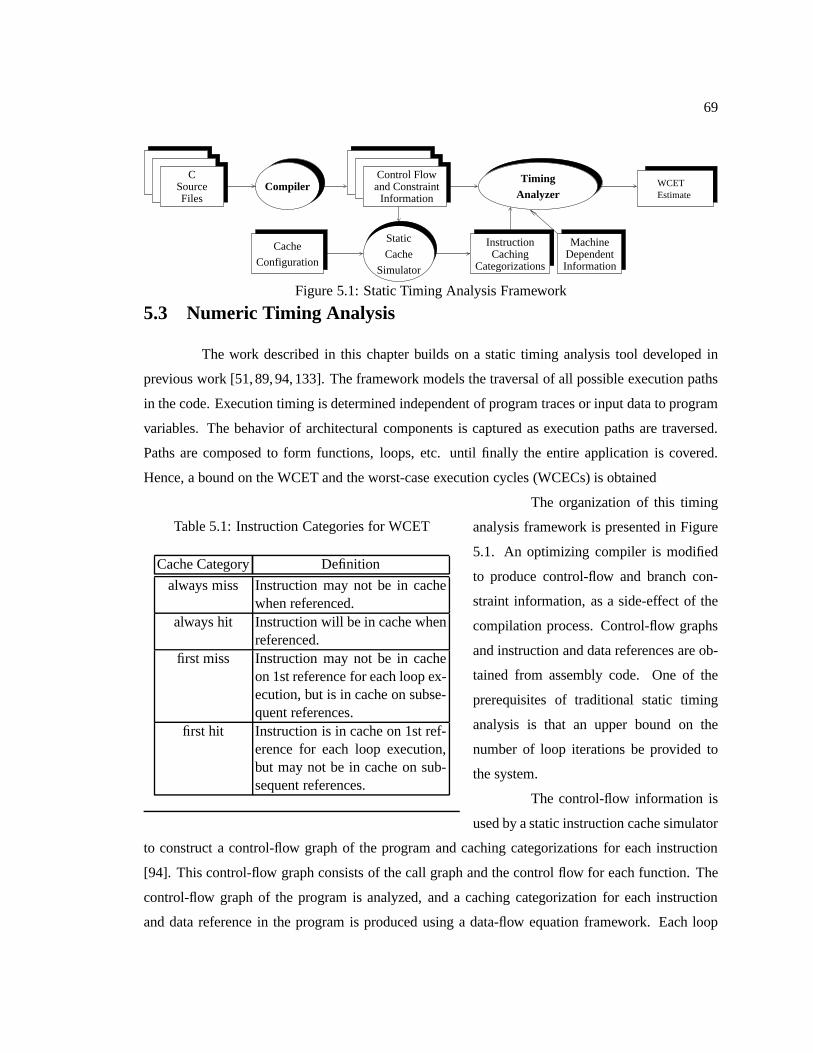
69

EstimateWCET

ConfigurationCaching

Simulator

Cache

Static

Source and ConstraintFiles

C Control Flow

Information

Cache

Categorizations

InstructionDependentMachine

Information

TimingAnalyzer

Compiler

Figure 5.1: Static Timing Analysis Framework

5.3 Numeric Timing Analysis

The work described in this chapter builds on a static timing analysis tool developed in

previous work [51,89,94,133]. The framework models the traversal of all possible execution paths

in the code. Execution timing is determined independent of program traces or input data to program

variables. The behavior of architectural components is captured as execution paths are traversed.

Paths are composed to form functions, loops, etc. until finally the entire application is covered.

Hence, a bound on the WCET and the worst-case execution cycles (WCECs) is obtained

Table 5.1: Instruction Categories for WCET

Cache Category Definition

always miss Instruction may not be in cachewhen referenced.

always hit Instruction will be in cache whenreferenced.

first miss Instruction may not be in cacheon 1st reference for each loop ex-ecution, but is in cache on subse-quent references.

first hit Instruction is in cache on 1st ref-erence for each loop execution,but may not be in cache on sub-sequent references.

The organization of this timing

analysis framework is presented in Figure

5.1. An optimizing compiler is modified

to produce control-flow and branch con-

straint information, as a side-effect of the

compilation process. Control-flow graphs

and instruction and data references are ob-

tained from assembly code. One of the

prerequisites of traditional static timing

analysis is that an upper bound on the

number of loop iterations be provided to

the system.

The control-flow information is

used by a static instruction cache simulator

to construct a control-flow graph of the program and caching categorizations for each instruction

[94]. This control-flow graph consists of the call graph and the control flow for each function. The

control-flow graph of the program is analyzed, and a caching categorization for each instruction

and data reference in the program is produced using a data-flow equation framework. Each loop

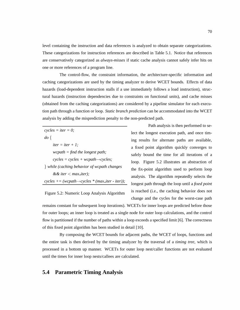
70

level containing the instruction and data references is analyzed to obtain separate categorizations.

These categorizations for instruction references are described in Table 5.1. Notice that references

are conservatively categorized asalways-missesif static cache analysis cannot safely infer hits on

one or more references of a program line.

The control-flow, the constraint information, the architecture-specific information and

caching categorizations are used by the timing analyzer to derive WCET bounds. Effects of data

hazards (load-dependent instruction stalls if a use immediately follows a load instruction), struc-

tural hazards (instruction dependencies due to constraints on functional units), and cache misses

(obtained from the caching categorizations) are considered by a pipeline simulator for each execu-

tion path through a function or loop.Static branch predictioncan be accommodated into the WCET

analysis by adding the misprediction penalty to the non-predicted path.

cycles = iter = 0;

do{

iter = iter + 1;

wcpath = find the longest path;

cycles = cycles + wcpath→cycles;

} while (caching behavior of wcpath changes

&& iter < max iter);

cycles += (wcpath→cycles * (maxiter - iter));

Figure 5.2: Numeric Loop Analysis Algorithm

Path analysis is then performed to se-

lect the longest execution path, and once tim-

ing results for alternate paths are available,

a fixed point algorithm quickly converges to

safely bound the time for all iterations of a

loop. Figure 5.2 illustrates an abstraction of

the fix-point algorithm used to perform loop

analysis. The algorithm repeatedly selects the

longest path through the loop until afixed point

is reached (i.e., the caching behavior does not

change and the cycles for the worst-case path

remains constant for subsequent loop iterations). WCETs for inner loops are predicted before those

for outer loops; an inner loop is treated as a single node for outer loop calculations, and the control

flow is partitioned if the number of paths within a loop exceeds a specified limit [6]. The correctness

of this fixed point algorithm has been studied in detail [10].

By composing the WCET bounds for adjacent paths, the WCET of loops, functions and

the entire task is then derived by the timing analyzer by the traversal of atiming tree, which is

processed in a bottom up manner. WCETs for outer loop nest/caller functions are not evaluated

until the times for inner loop nests/callees are calculated.

5.4 Parametric Timing Analysis

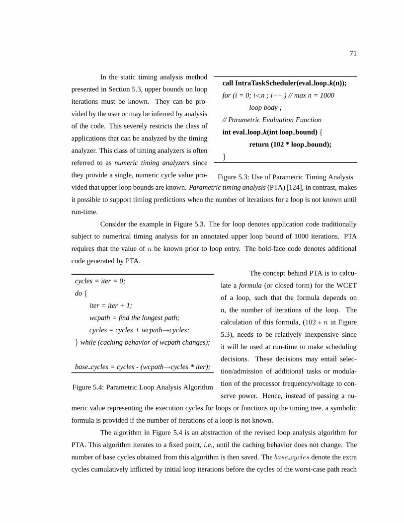
71

call IntraTaskScheduler(eval loop k(n));

for (i = 0; i <n ; i++ ) // max n = 1000

loop body ;

// Parametric Evaluation Function

int eval loop k(int loop bound) {

return (102 * loop bound);

}

Figure 5.3: Use of Parametric Timing Analysis

In the static timing analysis method

presented in Section 5.3, upper bounds on loop

iterations must be known. They can be pro-

vided by the user or may be inferred by analysis

of the code. This severely restricts the class of

applications that can be analyzed by the timing

analyzer. This class of timing analyzers is often

referred to asnumeric timing analyzerssince

they provide a single, numeric cycle value pro-

vided that upper loop bounds are known.Parametric timing analysis(PTA) [124], in contrast, makes

it possible to support timing predictions when the number ofiterations for a loop is not known until

run-time.

Consider the example in Figure 5.3. The for loop denotes application code traditionally

subject to numerical timing analysis for an annotated upperloop bound of 1000 iterations. PTA

requires that the value ofn be known prior to loop entry. The bold-face code denotes additional

code generated by PTA.

cycles = iter = 0;

do{

iter = iter + 1;

wcpath = find the longest path;

cycles = cycles + wcpath→cycles;

} while (caching behavior of wcpath changes);

basecycles = cycles - (wcpath→cycles * iter);

Figure 5.4: Parametric Loop Analysis Algorithm

The concept behind PTA is to calcu-

late aformula (or closed form) for the WCET

of a loop, such that the formula depends on

n, the number of iterations of the loop. The

calculation of this formula, (102 ∗ n in Figure

5.3), needs to be relatively inexpensive since

it will be used at run-time to make scheduling

decisions. These decisions may entail selec-

tion/admission of additional tasks or modula-

tion of the processor frequency/voltage to con-

serve power. Hence, instead of passing a nu-

meric value representing the execution cycles for loops or functions up the timing tree, a symbolic

formula is provided if the number of iterations of a loop is not known.

The algorithm in Figure 5.4 is an abstraction of the revised loop analysis algorithm for

PTA. This algorithm iterates to a fixed point,i.e., until the caching behavior does not change. The

number of base cycles obtained from this algorithm is then saved. Thebase cycles denote the extra

cycles cumulatively inflicted by initial loop iterations before the cycles of the worst-case path reach

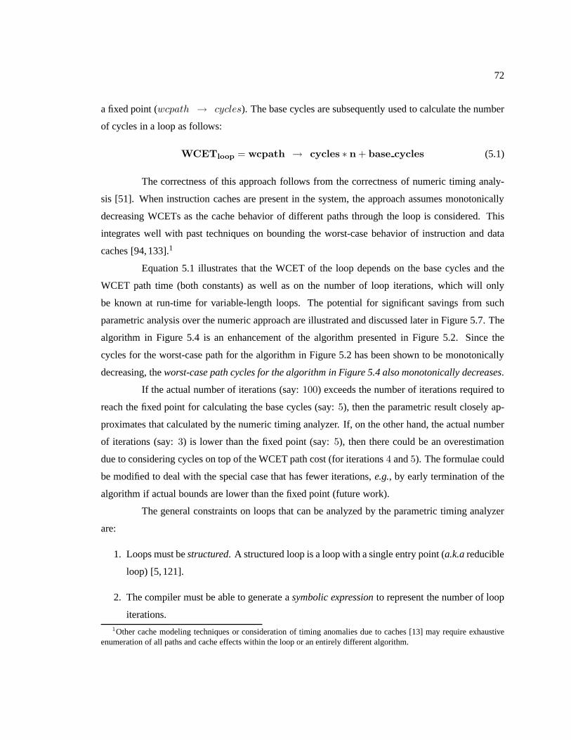
72

a fixed point (wcpath → cycles). The base cycles are subsequently used to calculate the number

of cycles in a loop as follows:

WCETloop = wcpath → cycles ∗ n + base cycles (5.1)

The correctness of this approach follows from the correctness of numeric timing analy-

sis [51]. When instruction caches are present in the system,the approach assumes monotonically

decreasing WCETs as the cache behavior of different paths through the loop is considered. This

integrates well with past techniques on bounding the worst-case behavior of instruction and data

caches [94,133].1

Equation 5.1 illustrates that the WCET of the loop depends onthe base cycles and the

WCET path time (both constants) as well as on the number of loop iterations, which will only

be known at run-time for variable-length loops. The potential for significant savings from such

parametric analysis over the numeric approach are illustrated and discussed later in Figure 5.7. The

algorithm in Figure 5.4 is an enhancement of the algorithm presented in Figure 5.2. Since the

cycles for the worst-case path for the algorithm in Figure 5.2 has been shown to be monotonically

decreasing, theworst-case path cycles for the algorithm in Figure 5.4 also monotonically decreases.

If the actual number of iterations (say:100) exceeds the number of iterations required to

reach the fixed point for calculating the base cycles (say:5), then the parametric result closely ap-

proximates that calculated by the numeric timing analyzer.If, on the other hand, the actual number

of iterations (say:3) is lower than the fixed point (say:5), then there could be an overestimation

due to considering cycles on top of the WCET path cost (for iterations4 and5). The formulae could

be modified to deal with the special case that has fewer iterations,e.g., by early termination of the

algorithm if actual bounds are lower than the fixed point (future work).

The general constraints on loops that can be analyzed by the parametric timing analyzer

are:

1. Loops must bestructured. A structured loop is a loop with a single entry point (a.k.areducible

loop) [5,121].

2. The compiler must be able to generate asymbolic expressionto represent the number of loop

iterations.1Other cache modeling techniques or consideration of timinganomalies due to caches [13] may require exhaustive

enumeration of all paths and cache effects within the loop oran entirely different algorithm.

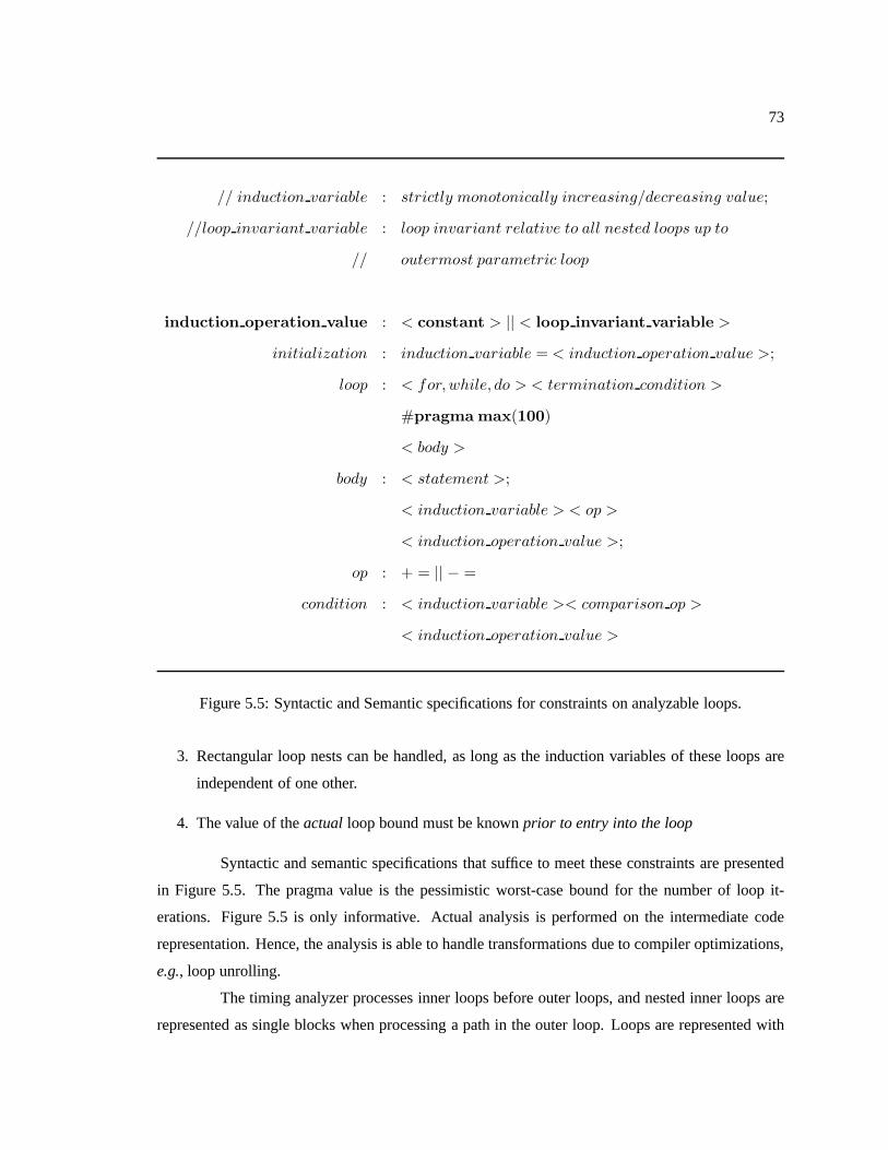
73

// induction variable : strictly monotonically increasing/decreasing value;

//loop invariant variable : loop invariant relative to all nested loops up to

// outermost parametric loop

induction operation value : < constant > || < loop invariant variable >

initialization : induction variable = < induction operation value >;

loop : < for,while, do > < termination condition >

#pragma max(100)

< body >

body : < statement >;

< induction variable > < op >

< induction operation value >;

op : + = || − =

condition : < induction variable >< comparison op >

< induction operation value >

Figure 5.5: Syntactic and Semantic specifications for constraints on analyzable loops.

3. Rectangular loop nests can be handled, as long as the induction variables of these loops are

independent of one other.

4. The value of theactual loop bound must be knownprior to entry into the loop

Syntactic and semantic specifications that suffice to meet these constraints are presented

in Figure 5.5. The pragma value is the pessimistic worst-case bound for the number of loop it-

erations. Figure 5.5 is only informative. Actual analysis is performed on the intermediate code

representation. Hence, the analysis is able to handle transformations due to compiler optimizations,

e.g., loop unrolling.

The timing analyzer processes inner loops before outer loops, and nested inner loops are

represented as single blocks when processing a path in the outer loop. Loops are represented with

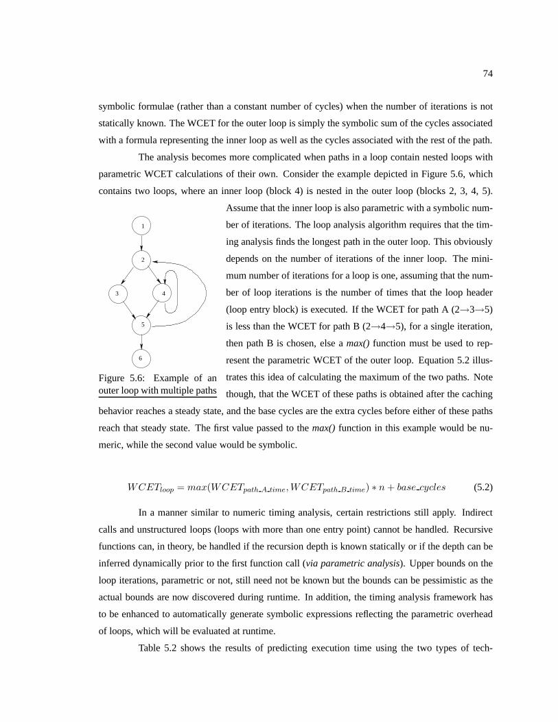
74

symbolic formulae (rather than a constant number of cycles)when the number of iterations is not

statically known. The WCET for the outer loop is simply the symbolic sum of the cycles associated

with a formula representing the inner loop as well as the cycles associated with the rest of the path.

The analysis becomes more complicated when paths in a loop contain nested loops with

parametric WCET calculations of their own. Consider the example depicted in Figure 5.6, which

contains two loops, where an inner loop (block 4) is nested inthe outer loop (blocks 2, 3, 4, 5).

2

5

6

1

3 4

Figure 5.6: Example of anouter loop with multiple paths

Assume that the inner loop is also parametric with a symbolicnum-

ber of iterations. The loop analysis algorithm requires that the tim-

ing analysis finds the longest path in the outer loop. This obviously

depends on the number of iterations of the inner loop. The mini-

mum number of iterations for a loop is one, assuming that the num-

ber of loop iterations is the number of times that the loop header

(loop entry block) is executed. If the WCET for path A (2→3→5)

is less than the WCET for path B (2→4→5), for a single iteration,

then path B is chosen, else amax() function must be used to rep-

resent the parametric WCET of the outer loop. Equation 5.2 illus-

trates this idea of calculating the maximum of the two paths.Note

though, that the WCET of these paths is obtained after the caching

behavior reaches a steady state, and the base cycles are the extra cycles before either of these paths

reach that steady state. The first value passed to themax() function in this example would be nu-

meric, while the second value would be symbolic.

WCETloop = max(WCETpath A time,WCETpath B time) ∗ n + base cycles (5.2)

In a manner similar to numeric timing analysis, certain restrictions still apply. Indirect

calls and unstructured loops (loops with more than one entrypoint) cannot be handled. Recursive

functions can, in theory, be handled if the recursion depth is known statically or if the depth can be

inferred dynamically prior to the first function call (via parametric analysis). Upper bounds on the

loop iterations, parametric or not, still need not be known but the bounds can be pessimistic as the

actual bounds are now discovered during runtime. In addition, the timing analysis framework has

to be enhanced to automatically generate symbolic expressions reflecting the parametric overhead

of loops, which will be evaluated at runtime.

Table 5.2 shows the results of predicting execution time using the two types of tech-

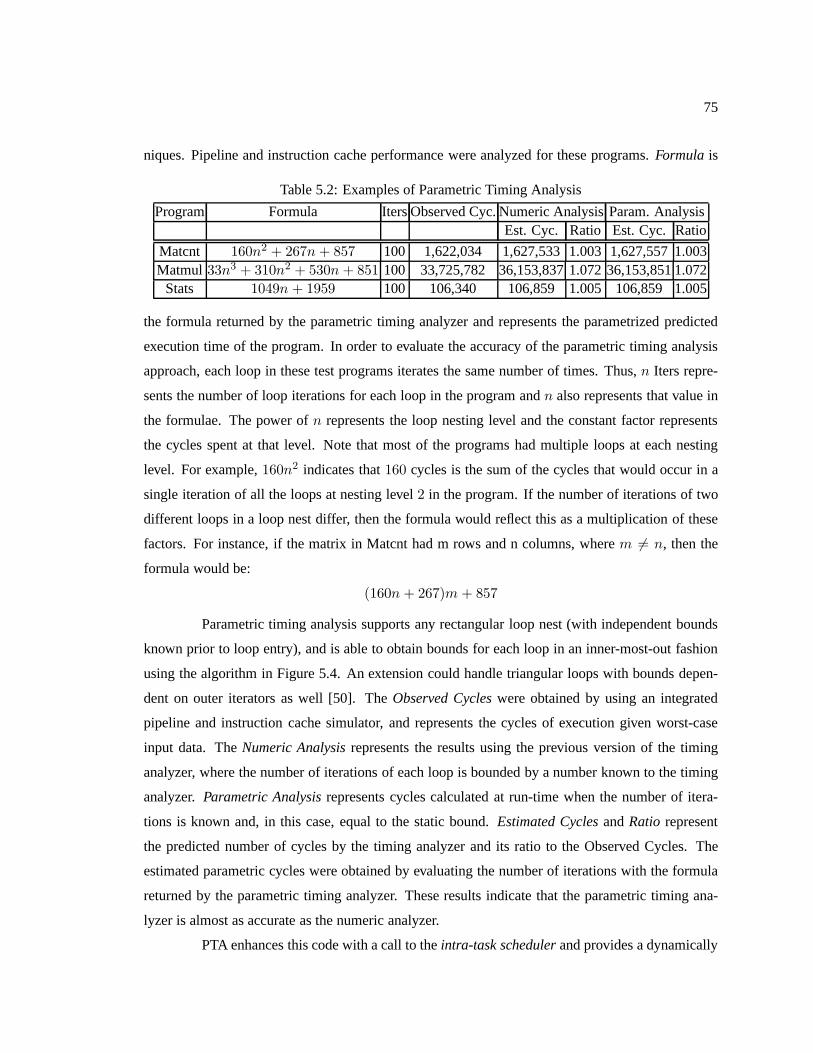
75

niques. Pipeline and instruction cache performance were analyzed for these programs.Formula is

Table 5.2: Examples of Parametric Timing Analysis

Program Formula ItersObserved Cyc.Numeric AnalysisParam. AnalysisEst. Cyc. Ratio Est. Cyc. Ratio

Matcnt 160n2 + 267n + 857 100 1,622,034 1,627,533 1.003 1,627,5571.003Matmul 33n3 + 310n2 + 530n + 851 100 33,725,782 36,153,8371.07236,153,8511.072

Stats 1049n + 1959 100 106,340 106,859 1.005 106,859 1.005

the formula returned by the parametric timing analyzer and represents the parametrized predicted

execution time of the program. In order to evaluate the accuracy of the parametric timing analysis

approach, each loop in these test programs iterates the samenumber of times. Thus,n Iters repre-

sents the number of loop iterations for each loop in the program andn also represents that value in

the formulae. The power ofn represents the loop nesting level and the constant factor represents

the cycles spent at that level. Note that most of the programshad multiple loops at each nesting

level. For example,160n2 indicates that160 cycles is the sum of the cycles that would occur in a

single iteration of all the loops at nesting level2 in the program. If the number of iterations of two

different loops in a loop nest differ, then the formula wouldreflect this as a multiplication of these

factors. For instance, if the matrix in Matcnt had m rows and ncolumns, wherem 6= n, then the

formula would be:

(160n + 267)m + 857

Parametric timing analysis supports any rectangular loop nest (with independent bounds

known prior to loop entry), and is able to obtain bounds for each loop in an inner-most-out fashion

using the algorithm in Figure 5.4. An extension could handletriangular loops with bounds depen-

dent on outer iterators as well [50]. TheObserved Cycleswere obtained by using an integrated

pipeline and instruction cache simulator, and represents the cycles of execution given worst-case

input data. TheNumeric Analysisrepresents the results using the previous version of the timing

analyzer, where the number of iterations of each loop is bounded by a number known to the timing

analyzer.Parametric Analysisrepresents cycles calculated at run-time when the number ofitera-

tions is known and, in this case, equal to the static bound.Estimated CyclesandRatio represent

the predicted number of cycles by the timing analyzer and itsratio to the Observed Cycles. The

estimated parametric cycles were obtained by evaluating the number of iterations with the formula

returned by the parametric timing analyzer. These results indicate that the parametric timing ana-

lyzer is almost as accurate as the numeric analyzer.

PTA enhances this code with a call to theintra-task schedulerand provides a dynamically

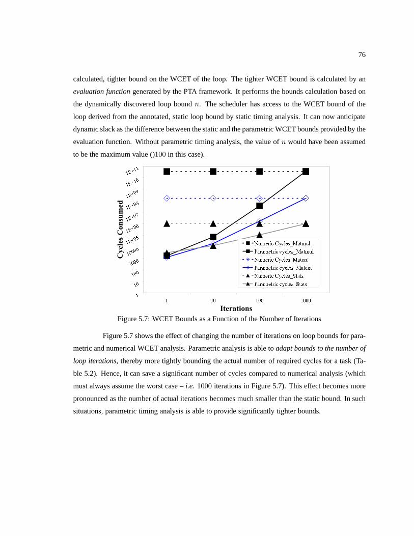
76

calculated, tighter bound on the WCET of the loop. The tighter WCET bound is calculated by an

evaluation functiongenerated by the PTA framework. It performs the bounds calculation based on

the dynamically discovered loop boundn. The scheduler has access to the WCET bound of the

loop derived from the annotated, static loop bound by statictiming analysis. It can now anticipate

dynamic slack as the difference between the static and the parametric WCET bounds provided by the

evaluation function. Without parametric timing analysis,the value ofn would have been assumed

to be the maximum value ()100 in this case).

��������������������������������������������������

�� �������������� ������ ��������������� ���� ��������������������� �������������������� �������������������� �����������������

Figure 5.7: WCET Bounds as a Function of the Number of Iterations

Figure 5.7 shows the effect of changing the number of iterations on loop bounds for para-

metric and numerical WCET analysis. Parametric analysis isable toadapt bounds to the number of

loop iterations, thereby more tightly bounding the actual number of required cycles for a task (Ta-

ble 5.2). Hence, it can save a significant number of cycles compared to numerical analysis (which

must always assume the worst case –i.e. 1000 iterations in Figure 5.7). This effect becomes more

pronounced as the number of actual iterations becomes much smaller than the static bound. In such

situations, parametric timing analysis is able to provide significantly tighter bounds.

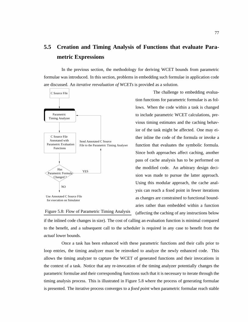
77

5.5 Creation and Timing Analysis of Functions that evaluatePara-

metric Expressions

In the previous section, the methodology for deriving WCET bounds from parametric

formulae was introduced. In this section, problems in embedding such formulae in application code

are discussed. Aniterative reevaluation of WCETsis provided as a solution.

Use Annotated C Source File

YES

NO

Has

C Source File

C Source FileAnnotated with

Parametric EvaluationFunctions

Parametric FormulaChanged ?

Send Annotated C SourceFile to the Parametric Timing Analyser

ParametricTiming Analyzer

for execution on Simulator

Figure 5.8: Flow of Parametric Timing Analysis

The challenge to embedding evalua-

tion functions for parametric formulae is as fol-

lows. When the code within a task is changed

to include parametric WCET calculations, pre-

vious timing estimates and the caching behav-

ior of the task might be affected. One may ei-

ther inline the code of the formula or invoke a

function that evaluates the symbolic formula.

Since both approaches affect caching, another

pass of cache analysis has to be performed on

the modified code. An arbitrary design deci-

sion was made to pursue the latter approach.

Using this modular approach, the cache anal-

ysis can reach a fixed point in fewer iterations

as changes are constrained to functional bound-

aries rather than embedded within a function

(affecting the caching of any instructions below

if the inlined code changes in size). The cost of calling an evaluation function is minimal compared

to the benefit, and a subsequent call to the scheduler is required in any case to benefit from the

actual lower bounds.

Once a task has been enhanced with these parametric functions and their calls prior to

loop entries, the timing analyzer must be reinvoked to analyze the newly enhanced code. This

allows the timing analyzer to capture the WCET of generated functions and their invocations in

the context of a task. Notice that any re-invocation of the timing analyzer potentially changes the

parametric formulae and their corresponding functions such that it is necessary to iterate through the

timing analysis process. This is illustrated in Figure 5.8 where the process of generating formulae

is presented. The iterative process converges to afixed pointwhen parametric formulae reach stable

78

Function

Function

Loop 2Loop 1

GeneratedAnalyzedNumericallyAnalyzed

AnalyzedNot Yet

Not Yet Not Yet

(a) Loop 2 contains a Symbolic number of iterations

Gen FunctionSource codegenerated

Not YetAnalyzed

Loop 1Numerically

Analyzed

Function

Loop 2

AnalyzedParametrically

(b) Loop 2 is analyzed and WCET Function is generated

Parametrically

Function

Analyzed

Loop 1Numerically

Analyzed

Loop 2

Analyzed

Not Yet

NumericallyAnalyzed

Gen Function

(c) Generated Function in Analyzed

Loop 1 Loop 2Numerically

Analysed

FunctionNumerically

Analysed

GenParametrically

Analyzed

FunctionParametrically

Analyzed

(d) Function containing code calling Generated Function is

analyzed

Figure 5.9: Example of using Parametric Timing Predictions

states. Typically, the parametric timing analysis and calculation of the parametric formulae takeless

than a secondto complete. Since this is an offline process, it does not add to the overhead of the

execution of the parametrized system.

An example is presented in Figure 5.9, where timing analysisis accomplished in stages,

as parametric formulae are generated and evaluated later. In the example shown, a function is

generated by the timing analyzer to calculate the WCET for loop 2, whose number of iterations is

only known at run-time. The following sequence of operations takes place:

1. A call to a function is inserted that returns the WCET for a specified loop or function based

on a parameter indicating the number of loop iterations thatis available at run time. The

instructions that are associated with the call and the ones that use the return value after the

call are generated during the initial compilation. For instance, in Figure 5.9(a) a function calls

the yet-to-be generated function to obtain the WCET of loop2, which contains the symbolic

number of iterations.

2. The timing analyzer generates the source code for the called function in a separate file when

processing the specified loop or function whose time needs tobe calculated at run time. For

instance, Figure 5.9(c) shows that after loop2 has been parametrically analyzed, the code for

the evaluation functionhas been generated. Note that the timing analysis tree representing

79

the loops and functions in the program is processed in abottom-upfashion. The code in the

function invoking the generated function is not evaluated until after the generated function is

produced. The static cache simulator can initially assume that a call to an unknown function

invalidates the entire cache. Figure 5.3 shows an example ofthe source code for such a

generated function.

3. The generated function is compiled and placed at the end ofthe executable. The formula

representing the symbolic WCET need not be simplified by the timing analyzer. Most opti-

mizing compilers perform constant folding, strength reduction, and other optimizations that

will automatically simplify the symbolic WCET produced by the timing analyzer. By plac-

ing the generated function after the rest of the program, instruction addresses of the program

remain unaffected. While the caching behavior may have changed, loops are unaffected since

the timing tree is processed in a bottom-up order.

4. The timing analyzer is invoked again to complete the analysis of the program, which now

includes calculating the WCET of the generated function andthe code invoking this function.

For instance, Figure 5.9(c) shows that the generated function has been numerically analyzed

and Figure 5.9(d) shows that the original function has been parametrically analyzed, which

now includes the numeric WCET required for executing the newfunction.

In short, this approach allows for timing analysis to proceed in stages. Parametric formu-

lae are produced when needed and source code functions representing these formulae are produced,

which are also subsequently compiled, inserted into the task code and analyzed. This process con-

tinues until a formula is obtained for the entire program or task.

5.6 Using Parametric Expressions

In this section, potential benefits of parametric formulae and their evaluation functions are

discussed. A more accurate knowledge of the remaining execution time provides a scheduler with

information about additional slack in the schedule. This slack can be utilized in multiple ways:

• A dynamic admission scheduler can accept additional real-time tasks due to parametric bounds

of the WCET of a task, which become tighter as execution progresses.

• Dynamic slack can also be used fordynamic voltage (and frequency) scaling (DVS) in order

to reduce power.

80

In the remainder of this chapter, the latter case will be detailed.

Recall that parametric timing analysis involves the integration of symbolic WCET formu-

lae as functions and their respective evaluation calls intoa task’s code. Apart from these inserted

function calls, calls to transfer control to the DVS component of an optional dynamic scheduler are

also insertedbeforeentering parametric loops, as shown in Figure 5.3. The parametric expressions

are evaluated at run-time (using evaluation functions similar to the one in the figure) as knowledge

of actual loops bounds becomes available. The newly calculated tighter bound on the execution time

for the parametric loop is passed along to the scheduler. Thescheduler is able to determine newly

found dynamic slack by comparing worst-case execution cycles (WCECs) for that particular loop

with the parametrically bounded execution time. The WCECs for each loop and the task as a whole

are provided to the scheduler by the static timing analysis toolset. Static loop bounds for each loop

are provided by hand. Automatic detection of bounds is subject to future work.

Dynamic slackoriginating from the evaluation of parametric expressionsat run-time is

discovered and can be exploited by the scheduler for admission scheduling or DVS (see above).

This work is unique in that it exploits early knowledge of parametric loop bounds, thus allowing

the possibility to tightly bound the overall execution of the remainderof the task. To this effect, an

intra-task DVS algorithm has been developed, to lower processor frequency and voltage. Another

unique aspect of this approach is that every successive parametric loop that is encountered during

the execution of the task potentially provides more slack and, hence, allows the system to further

scale down the processor frequency. This is in sharp contrast to past real-time schemes where DVS-

regulated tasks are sped up as execution progresses, mainlydue to approaching deadlines.

5.7 Framework

An overview of the experimental framework is depicted in Figure 5.10. The instruction

information fed to the timing analyzer is obtained from the P-compiler, which preprocesses gcc-

generated PISA assembly. The C source files are also fed simultaneously to both the static and the

parametric timing analyzers. Safe (but, due to the parametric nature of loops, not necessarily tight)

upper bounds for loops are provided as inputs to the static timing analyzer (STA). The worst-case

execution times/cycles, for tasks as well as loops, provided by the STA are provided as input to a

scheduler. The C source files are also provided to the PTA. ThePTA produces source files annotated

with parametric evaluation functions as well as calls to transfer control to the schedulerbeforeentry

into a parametric loop. These annotated source files form thetask set for execution by the scheduler.

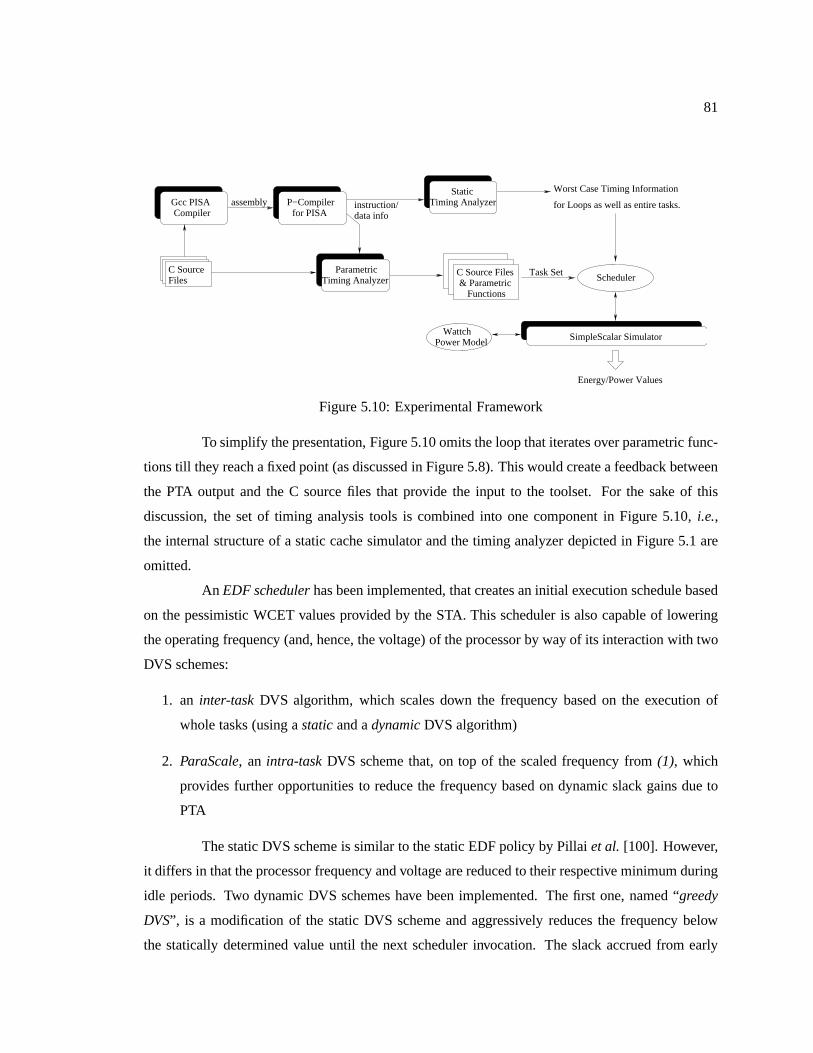
81

C SourceFiles

instruction/Gcc PISACompiler

P−Compilerfor PISA

assembly

Parametric

Static

Functions& ParametricC Source Files Task Set

WattchPower Model SimpleScalar Simulator

for Loops as well as entire tasks.

Worst Case Timing Information

Energy/Power Values

data infoTiming Analyzer

Timing Analyzer Scheduler

Figure 5.10: Experimental Framework

To simplify the presentation, Figure 5.10 omits the loop that iterates over parametric func-

tions till they reach a fixed point (as discussed in Figure 5.8). This would create a feedback between

the PTA output and the C source files that provide the input to the toolset. For the sake of this

discussion, the set of timing analysis tools is combined into one component in Figure 5.10,i.e.,

the internal structure of a static cache simulator and the timing analyzer depicted in Figure 5.1 are

omitted.

An EDF schedulerhas been implemented, that creates an initial execution schedule based

on the pessimistic WCET values provided by the STA. This scheduler is also capable of lowering

the operating frequency (and, hence, the voltage) of the processor by way of its interaction with two

DVS schemes:

1. an inter-taskDVS algorithm, which scales down the frequency based on the execution of

whole tasks (using astaticand adynamicDVS algorithm)

2. ParaScale, an intra-taskDVS scheme that, on top of the scaled frequency from(1), which

provides further opportunities to reduce the frequency based on dynamic slack gains due to

PTA

The static DVS scheme is similar to the static EDF policy by Pillai et al. [100]. However,

it differs in that the processor frequency and voltage are reduced to their respective minimum during

idle periods. Two dynamic DVS schemes have been implemented. The first one, named “greedy

DVS”, is a modification of the static DVS scheme and aggressivelyreduces the frequency below

the statically determined value until the next scheduler invocation. The slack accrued from early

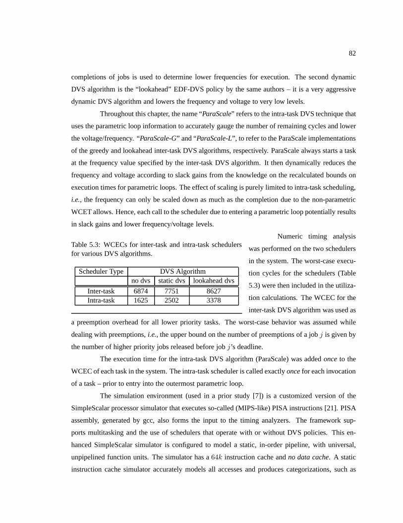
82

completions of jobs is used to determine lower frequencies for execution. The second dynamic

DVS algorithm is the “lookahead” EDF-DVS policy by the same authors – it is a very aggressive

dynamic DVS algorithm and lowers the frequency and voltage to very low levels.

Throughout this chapter, the name “ParaScale” refers to the intra-task DVS technique that

uses the parametric loop information to accurately gauge the number of remaining cycles and lower

the voltage/frequency. “ParaScale-G” and “ParaScale-L”, to refer to the ParaScale implementations

of the greedy and lookahead inter-task DVS algorithms, respectively. ParaScale always starts a task

at the frequency value specified by the inter-task DVS algorithm. It then dynamically reduces the

frequency and voltage according to slack gains from the knowledge on the recalculated bounds on

execution times for parametric loops. The effect of scalingis purely limited to intra-task scheduling,

i.e., the frequency can only be scaled down as much as the completion due to the non-parametric

WCET allows. Hence, each call to the scheduler due to entering a parametric loop potentially results

in slack gains and lower frequency/voltage levels.

Table 5.3: WCECs for inter-task and intra-task schedulersfor various DVS algorithms.

Scheduler Type DVS Algorithmno dvs static dvs lookahead dvs

Inter-task 6874 7751 8627Intra-task 1625 2502 3378

Numeric timing analysis

was performed on the two schedulers

in the system. The worst-case execu-

tion cycles for the schedulers (Table

5.3) were then included in the utiliza-

tion calculations. The WCEC for the

inter-task DVS algorithm was used as

a preemption overhead for all lower priority tasks. The worst-case behavior was assumed while

dealing with preemptions,i.e., the upper bound on the number of preemptions of a jobj is given by

the number of higher priority jobs released before jobj’s deadline.

The execution time for the intra-task DVS algorithm (ParaScale) was addedonceto the

WCEC of each task in the system. The intra-task scheduler is called exactlyoncefor each invocation

of a task – prior to entry into the outermost parametric loop.

The simulation environment (used in a prior study [7]) is a customized version of the

SimpleScalar processor simulator that executes so-called(MIPS-like) PISA instructions [21]. PISA

assembly, generated by gcc, also forms the input to the timing analyzers. The framework sup-

ports multitasking and the use of schedulers that operate with or without DVS policies. This en-

hanced SimpleScalar simulator is configured to model a static, in-order pipeline, with universal,

unpipelined function units. The simulator has a64k instruction cache andno data cache. A static

instruction cache simulator accurately models all accesses and produces categorizations, such as

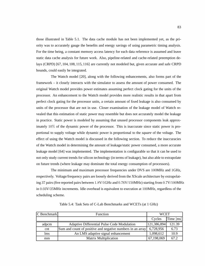
83

those illustrated in Table 5.1. The data cache module has notbeen implemented yet, as the pri-

ority was to accurately gauge the benefits and energy savingsof using parametric timing analysis.

For the time being, a constant memory access latency for eachdata reference is assumed and leave

static data cache analysis for future work. Also, pipeline-related and cache-related preemption de-

lays (CRPD) [67, 104, 108, 115, 116] are currently not modeled but, given accurate and safe CRPD

bounds, could easily be integrated.

The Wattch model [20], along with the following enhancements, also forms part of the

framework – it closely interacts with the simulator to assess the amount of power consumed. The

original Wattch model provides power estimates assuming perfect clock gating for the units of the

processor. An enhancement to the Wattch model provides morerealistic results in that apart from

perfect clock gating for the processor units, a certain amount of fixed leakage is also consumed by

units of the processor that are not in use. Closer examination of the leakage model of Wattch re-

vealed that this estimation of static power may resemble butdoes not accurately model the leakage

in practice. Static power is modeled by assuming that unusedprocessor components leak approx-

imately 10% of the dynamic power of the processor. This is inaccurate since static power is pro-

portional to supply voltage while dynamic power is proportional to thesquareof the voltage. The

effect of using the Wattch model is discussed in the following section. To reduce the inaccuracies

of the Wattch model in determining the amount of leakage/static power consumed, a more accurate

leakage model [64] was implemented. The implementation is configurable so that it can be used to

not only study current trends for silicon technology (in terms of leakage), but also able to extrapolate

on future trends (where leakage may dominate the total energy consumption of processors).

The minimum and maximum processor frequencies under DVS are100MHz and1GHz,

respectively. Voltage/frequency pairs are loosely derived from the XScale architecture by extrapolat-

ing37 pairs (five reported pairs between1.8V/1GHz and0.76V/150MHz) starting from0.7V/100MHz

in 0.03V/25MHz increments. Idle overhead is equivalent to execution at100MHz, regardless of the

scheduling scheme.

Table 5.4: Task Sets of C-Lab Benchmarks and WCETs (at 1 GHz)

C Benchmark Function WCETCycles Time [ms]

adpcm Adaptive Differential Pulse Code Modulation 121,386,894 121.39cnt Sum and count of positive and negative numbers in an array6,728,956 6.73lms An LMS adaptive signal enhancement 1,098,612 10.9mm Matrix Multiplication 67,198,069 67.2

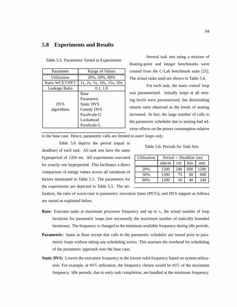
84

5.8 Experiments and Results

Table 5.5: Parameters Varied in Experiments

Parameter Range of Values

Utilization 20%, 50%, 80%Ratio WCET/PET 1x, 2x, 5x, 10x, 15x, 20x

Leakage Ratio 0.1, 1.0BaseParametric

DVS Static DVSalgorithms Greedy DVS

ParaScale-GLookaheadParaScale-L

Several task sets using a mixture of

floating-point and integer benchmarks were

created from the C-Lab benchmark suite [25].

The actual tasks used are shown in Table 5.4.

For each task, the main control loop

was parametrized. Initially loops at all nest-

ing levels were parametrized, but diminishing

returns were observed as the levels of nesting

increased. In fact, the large number of calls to

the parametric scheduler due to nesting had ad-

verse effects on the power consumption relative

to the base case. Hence, parametric calls are limited toouter loops only.

Table 5.6: Periods for Task Sets

Utilization Period= Deadline[ms]adpcm cnt lms mm

20% 1200 240 600 120050% 1200 75 60 60080% 1200 50 40 240

Table 5.6 depicts the period (equal to

deadline) of each task. All task sets have the same

hyperperiod of1200 ms. All experiments executed

for exactly one hyperperiod. This facilitates a direct

comparison of energy values across all variations of

factors mentioned in Table 5.5. The parameters for

the experiments are depicted in Table 5.5. The uti-

lization, the ratio of worst-case to parametric execution times (PETs), and DVS support as follows

are varied as explained below.

Base: Executes tasks at maximum processor frequency and up ton, the actual number of loop

iterations for parametric loops (not necessarily the maximum number of statically bounded

iterations). The frequency is changed to the minimum available frequency during idle periods.

Parametric: Same as Base except that calls to the parametric scheduler are issued prior to para-

metric loops without taking any scheduling action. This assesses the overhead for scheduling

of the parametric approach over the base case.

Static DVS: Lowers the execution frequency to the lowest valid frequency based on system utiliza-

tion. For example, at80% utilization, the frequency chosen would be80% of the maximum

frequency. Idle periods, due to early task completion, are handled at the minimum frequency.

85

Greedy DVS: This scheme is similar to static DVS in that it starts with thestatically fixed fre-

quency but then aggressively lowers the frequency for thecurrent time periodbased on ac-

crued slack from previous task invocations. Every time a jobcompletes early, the slack gained

is passed on to the job which follows immediately. Let jobi be the job that completes early

and generates slack and let jobj be the job which follows (consumer). The greedy DVS

algorithm calculates the frequency of execution,α′, for j as follows:

α′ =

[

α ∗ Cj

α ∗ Cj + slacki

]

α (5.3)

whereα is the frequency determined by the static DVS scheme. Noticethat (a) this slack is

“lost” or rather reset to zero when the next scheduling decision takes place and(b) Equation

5.3 ensures that the new frequency scales down jobj so that it attempts to completely utilize

the slack from the previous job, but it does not stretch beyond the time originally budgeted for

its execution based on the higher, statically determined, frequency. From (a) and (b) above,

it can be seen that the new DVS scheme will never miss a deadline if the original static DVS

scheme never misses a deadline since greedy DVS accomplishes at least the same amount

of work as before. Hence, it never utilizes processor time which lies beyond the original

completion time of taskj. The processor switches to the lowest possible frequency/voltage

during idle time.

ParaScale-G: Combines the greedy and intra-task DVS schemes so that jobs start their execution

at the lowest valid frequency based on system utilization. Before a parametric loop is entered

the frequency is scaled down further according to the difference between the WCET bound

of the loop and the parametric bound of the loop calculated dynamically. ParaScale-G also

exploits savings due to already completed execution relative to the WCET for frequency scal-

ing. (These savings are small compared to the savings of parametric loops since parametric

loops generally occur early in the code). It also utilizes job slack accrued from previous task

invocations to further reduce the frequency. As in the case of the Static and Greedy DVS

schemes, the processor switches to the lowest possible frequency/voltage during idle time.

Lookahead: Implements an enhanced version [139] of Pillai’s [100]lookaheadEDF-DVS algo-

rithm – a very aggressive dynamic DVS algorithm.

ParaScale-L: Combines the lookahead and intra-task DVS which utilizes parametric loop informa-

tion. It is similar in operation to ParaScale-G. While ParaScale-G uses static values for initial

frequencies, ParaScale-L uses frequencies calculated by the aggressive, dynamic EDF-DVS

86

algorithm (lookahead).

Notice that all scheduling cases result in thesame amount of workbeing executed during

the hyperperiod (or any integer multiple thereof) due to theperiodic nature of the real-time work-

load. Hence, to assess the benefits in terms of power awareness, the energy consumed over such a

fixed period of time can be measured and compares between scheduling modes.

The scheduler overhead for the greedy DVS scheme differs from those of the static DVS

scheme by only a few cycles, as the only additional overhead is the calculation to determineα′

(Equation 5.3). This calculation is performed only once perscheduler invocation because the new

frequency only needs to be calculated for the next scheduledtask instance. Three types of energy

measurements are carried out during the course of the experiments:

PCG: Energy used withperfectclock gating (PCG) – only processor units that are used during

execution contribute to the energy measurements. This isolates the effect of the parametric

approach ondynamic power.

PCGL: Energy consumed byleakage only, based on prior methods [64]. This attempts to capture

the amount of energy exclusively used due to leakage.

PCGL-W: Energy used with perfect clock gating for the processor units includingleakage. Leak-

age power is modeled by Wattch as10% of dynamic power, which is not completely correct,

as discussed before.

The ratio of worst-case to actual (parametric) execution times is varied to study the effect

of variations in execution times and make the experimental results more realistic. More often than

not, the worst-case analysis of systems results in overestimations of WCET. ParaScale can take

advantage of this to obtain additional energy savings.

As part of the setup for the experiments PCGL leakage model’soperating parameters were

initialized with the ratio of leakage to dynamic power for one particular experimental point. The

ratio of dynamic and leakage energies for the WCET overestimation of1x and utilization of50%

was chosen for this purpose. This ratio was used to set up appropriate operating parameters (number

of transistors, body bias voltage,etc.), after which the experiments were allowed to execute freely

to completion. This provides a unique opportunity to study the effects of leakage for(a) current

processor technologies, where the ratio of leakage to dynamic are close to1 : 10 and (b) future

trends where the leakage may increase significantly as the above ratio approaches1 : 1. The

“leakage ratios” mentioned in table 5.5 refer to these two settings.

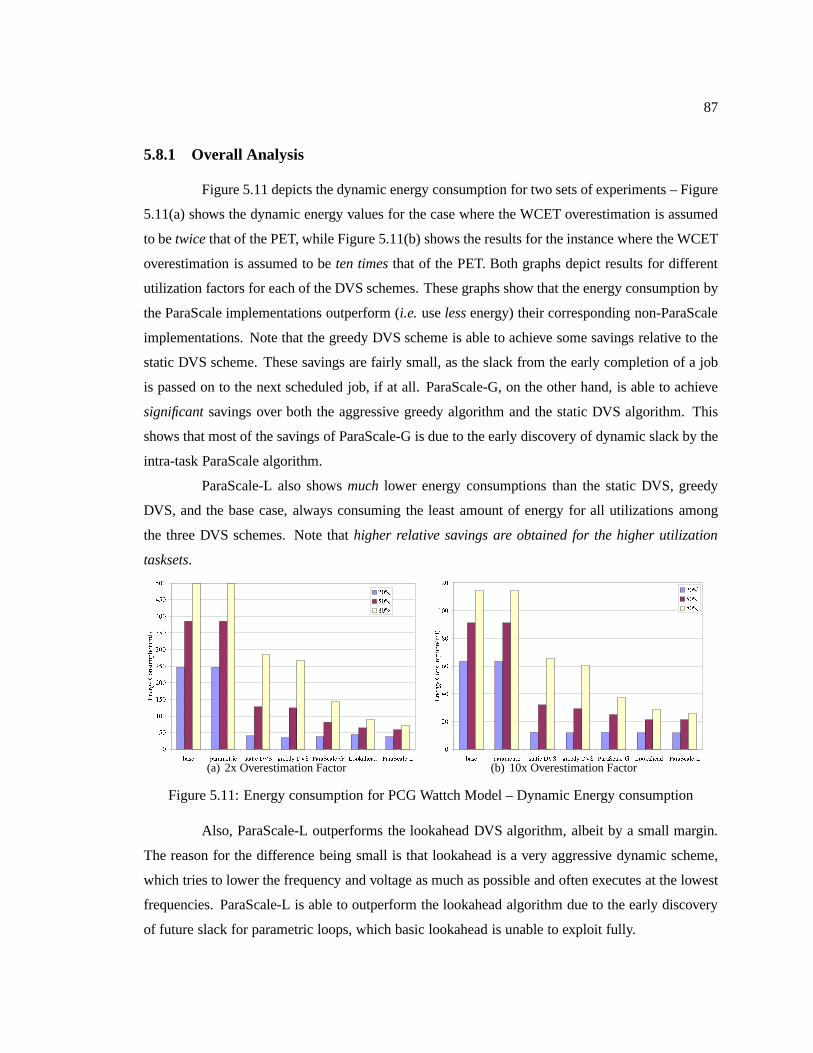
87

5.8.1 Overall Analysis

Figure 5.11 depicts the dynamic energy consumption for two sets of experiments – Figure

5.11(a) shows the dynamic energy values for the case where the WCET overestimation is assumed

to betwicethat of the PET, while Figure 5.11(b) shows the results for the instance where the WCET

overestimation is assumed to beten timesthat of the PET. Both graphs depict results for different

utilization factors for each of the DVS schemes. These graphs show that the energy consumption by

the ParaScale implementations outperform (i.e. uselessenergy) their corresponding non-ParaScale

implementations. Note that the greedy DVS scheme is able to achieve some savings relative to the

static DVS scheme. These savings are fairly small, as the slack from the early completion of a job

is passed on to the next scheduled job, if at all. ParaScale-G, on the other hand, is able to achieve

significantsavings over both the aggressive greedy algorithm and the static DVS algorithm. This

shows that most of the savings of ParaScale-G is due to the early discovery of dynamic slack by the

intra-task ParaScale algorithm.

ParaScale-L also showsmuch lower energy consumptions than the static DVS, greedy

DVS, and the base case, always consuming the least amount of energy for all utilizations among

the three DVS schemes. Note thathigher relative savings are obtained for the higher utilization

tasksets.

������������������������������

������� ���� � ������������������������������������������ !"#$%�&'()*+%�,(-.��/��/0�/

(a) 2x Overestimation Factor

121314151611621

789:;8<8=:><?@9>8>?@ABCD<::EFABCG8<8C@8H:IJKLLM8N:8EG8<8C@8H:IKOPQRSTUVPWXYZ[\VP]Y_ 21a151

(b) 10x Overestimation Factor

Figure 5.11: Energy consumption for PCG Wattch Model – Dynamic Energy consumption

Also, ParaScale-L outperforms the lookahead DVS algorithm, albeit by a small margin.

The reason for the difference being small is that lookahead is a very aggressive dynamic scheme,

which tries to lower the frequency and voltage as much as possible and often executes at the lowest

frequencies. ParaScale-L is able to outperform the lookahead algorithm due to the early discovery

of future slack for parametric loops, which basic lookaheadis unable to exploit fully.

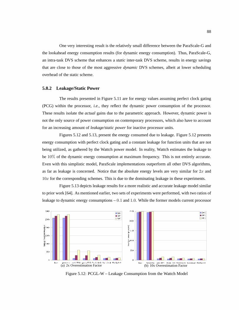
88

One very interesting result is the relatively small difference between the ParaScale-G and

the lookahead energy consumption results (for dynamic energy consumption). Thus, ParaScale-G,

an intra-task DVS scheme that enhances astatic inter-task DVS scheme, results in energy savings

that are close to those of the most aggressivedynamicDVS schemes, albeit at lower scheduling

overhead of the static scheme.

5.8.2 Leakage/Static Power

The results presented in Figure 5.11 are for energy values assuming perfect clock gating

(PCG) within the processor,i.e., they reflect the dynamic power consumption of the processor.

These results isolate theactualgains due to the parametric approach. However, dynamic power is

not the only source of power consumption on contemporary processors, which also have to account

for an increasing amount ofleakage/static powerfor inactive processor units.

Figures 5.12 and 5.13, present the energy consumed due to leakage. Figure 5.12 presents

energy consumption with perfect clock gating and a constantleakage for function units that are not

being utilized, as gathered by the Wattch power model. In reality, Wattch estimates the leakage to

be10% of the dynamic energy consumption at maximum frequency. This is not entirely accurate.

Even with this simplistic model, ParaScale implementations outperform all other DVS algorithms,

as far as leakage is concerned. Notice that the absolute energy levels are very similar for2x and

10x for the corresponding schemes. This is due to the dominatingleakage in these experiments.

Figure 5.13 depicts leakage results for a more realistic andaccurate leakage model similar

to prior work [64]. As mentioned earlier, two sets of experiments were performed, with two ratios of

leakage to dynamic energy consumptions –0.1 and1.0. While the former models current processor

������������������������

��������� ����� �������������������������������������������� !"#$�%&'()*$�+',- ./01/02/0

(a) 2x Overestimation Factor

34335333543363336433

789:;8<8=:><?@9>8>?@ABCD<::EFABCG8<8C@8H:IJKLLM8N:8EG8<8C@8H:IKOPQRSTUVPWXYZ[\VP]Y_ abcabdab

(b) 10x Overestimation Factor

Figure 5.12: PCGL-W – Leakage Consumption from the Wattch Model

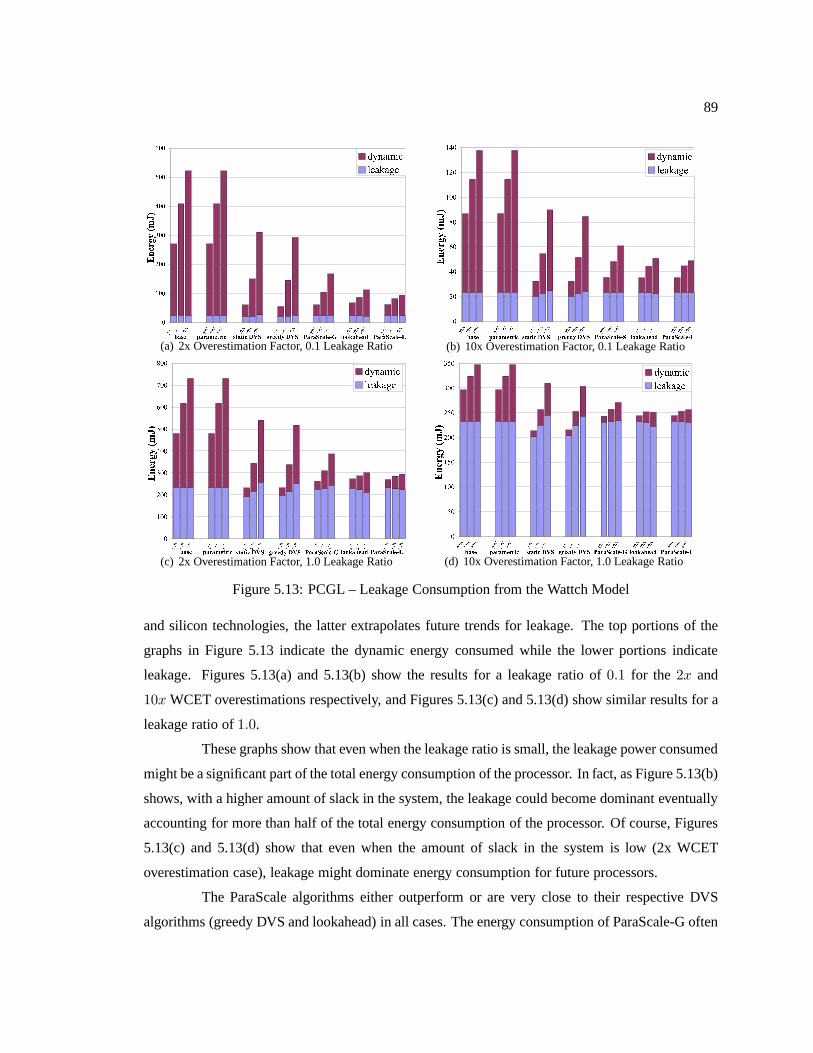
89

�������������������

������������������������������������ �������������������� �

!"#$%"&"'$(&)*#("()*+,-."&"-*"/$01/223"4$"5."&"-*"/$067&$$58+,-(a) 2x Overestimation Factor, 0.1 Leakage Ratio

9:9;9<9=9>99>:9>;9

?@AB@AC@A?@AB@AC@A?@AB@AC@A?@AB@AC@A?@AB@AC@A?@AB@AC@A?@AB@AC@ADEFGHIJKLMNOPQRSTUVQWQXV

YZ[\]ZZ_\ab[ZabcdefZZebZg\hegiijZk\ZlfZZebZg\hmn\\locde(b) 10x Overestimation Factor, 0.1 Leakage Ratio

pqpprppspptppuppvppwppxpp

yz{|z{}z{yz{|z{}z{yz{|z{}z{yz{|z{}z{yz{|z{}z{yz{|z{}z{yz{|z{}z{~�����������������������

����������������������� ������¡�¢£¡¤¤¥�¦��§ ������¡�¢©���§ª���(c) 2x Overestimation Factor, 1.0 Leakage Ratio

«¬«­««­¬«®««®¬«««¬«

°±²³±²±²°±²³±²±²°±²³±²±²°±²³±²±²°±²³±²±²°±²³±²±²°±²³±²±²µ¶·¹º»¼½¾¿ÀÁÂÃÄÅÆÇÂÈÂÉÇ

ÊËÌÍÎËÏËÐÍÑÏÒÓÌÑËÑÒÓÔÕÖ×ËÏËÖÓËØÍÙÚØÛÛÜËÝÍËÞ×ËÏËÖÓËØÍÙßàÏÍÍÞáÔÕÖ(d) 10x Overestimation Factor, 1.0 Leakage Ratio

Figure 5.13: PCGL – Leakage Consumption from the Wattch Model

and silicon technologies, the latter extrapolates future trends for leakage. The top portions of the

graphs in Figure 5.13 indicate the dynamic energy consumed while the lower portions indicate

leakage. Figures 5.13(a) and 5.13(b) show the results for a leakage ratio of0.1 for the 2x and

10x WCET overestimations respectively, and Figures 5.13(c) and 5.13(d) show similar results for a

leakage ratio of1.0.

These graphs show that even when the leakage ratio is small, the leakage power consumed

might be a significant part of the total energy consumption ofthe processor. In fact, as Figure 5.13(b)

shows, with a higher amount of slack in the system, the leakage could become dominant eventually

accounting for more than half of the total energy consumption of the processor. Of course, Figures

5.13(c) and 5.13(d) show that even when the amount of slack inthe system is low (2x WCET

overestimation case), leakage might dominate energy consumption for future processors.

The ParaScale algorithms either outperform or are very close to their respective DVS

algorithms (greedy DVS and lookahead) in all cases. The energy consumption of ParaScale-G often

90

results in energy consumption similar to that of the dynamiclookahead DVS algorithm. This holds

true for leakage as well as the total energy consumption (dynamic+leakage). Also, the combination

of lookahead and the inter-task ParaScale (ParaScale-L) outperforms all other implementations.

The graphs in Figure 5.13 indicate identical static energy consumptions for all utilizations

for the base and parametric experiments. The DVS algorithms, on the other hand, leak different

amounts of static power for each of the utilizations. This effect is due to the fact that leakage

depends on the actual voltage in the system. The static DVS algorithm consumes more leakage with

increasing systems utilizations since it executes at higher, statically determined frequencies (and,

hence, voltages) for higher utilizations. The greedy scheme performsslightly better as it is able to

lower the frequency of execution due to slack passing between consecutive jobs. The lookahead

and all ParaScale algorithms are able to aggressively lowertheir frequencies and voltage. Thus,

they have a different leakage pattern compared to the constant values seen for the non-DVS cases

or the increasing pattern for static DVS.

5.8.3 WCET/PET Ratio, Utilization Changes and Other Trends

Consider the effects of changing the WCET overestimation factor and utilization on en-

ergy consumption. The ParaScale-G algorithm is used as a case study and compare it to static DVS

and the base cases as depicted in Figures 5.11.

These graphs show slightly smaller relative energy savingsfor higher WCET factors (10x)

compared to lower ones (2x). This is due to the fact that more slack is available in the system for

the static algorithm to reduce frequency and voltage. Irrespective of the overestimation factor,

ParaScale-L performs best for all utilizations, as discussed further in this section. The absolute

energy level of2x overestimation is about3.5 times that of the10x case without considering leakage

for the highest utilization.

Furthermore, the ParaScale technique performs better for higher utilizations, as seen for

experiments with80% utilization in Figure 5.11(a). As the ParaScale technique is able to take

advantage of intra-task scheduling based on knowledge about past as well as future execution for a

task, it is able to lower the frequency more aggressively than other DVS algorithms. This is more

noticeable for higher utilization tasksets because less static slack is available to static algorithms for

frequency scaling.

Figure 5.14 shows the trends in energy consumption across WCET/PET ratios ranging

from 1x (no overestimation) to20x (large overestimation). Energy values for both DVS algorithms,

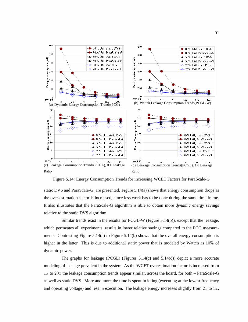
91

�������������������

������������������ ������ ������� ���� ��� !"#$%!&!"'()*��� !"#$+&,&*'&#-./0�� !"#$%!&!"'()*0�� !"#$+&,&*'&#-./1�� !"#$%!&!"'()*1�� !"#$+&,&*'&#-./

(a) Dynamic Energy Consumption Trends(PCG)

232242252262272227322

783898728798328:;<=>?@ABCDE?FGHIJKE?LHMN OPQRSTUVWSXSTYZ[\OPQRSTUV]XX\YXU_abPQRSTUVWSXSTYZ[\bPQRSTUV]XX\YXU_acPQRSTUVWSXSTYZ[\cPQRSTUV]XX\YXU_a(b) Wattch Leakage Consumption Trends(PCGL-W)

defdfegdgehd

figieifdifeigdijklmnopqrstuovwxyz{uo|x}~ ������������������������������������������������������������������������������������������������������������

(c) Leakage Consumption Trends(PCGL), 0.1 Leakage

Ratio

������������������

��������������������� ¡¢£¤¥�¦§©ª«¥�¬­® °±²³µ¶·³³¹º»¼°±²³µ¶½¾¼¹µ¿ÀÁ°±²³µ¶·³³¹º»¼Â°±²³µ¶½¾¼¹µ¿ÀÁð±²³µ¶·³³¹º»¼Ã°±²³µ¶½¾¼¹µ¿ÀÁ

(d) Leakage Consumption Trends(PCGL), 1.0 Leakage

Ratio

Figure 5.14: Energy Consumption Trends for increasing WCETFactors for ParaScale-G

static DVS and ParaScale-G, are presented. Figure 5.14(a) shows that energy consumption drops as

the over-estimation factor is increased, since less work has to be done during the same time frame.

It also illustrates that the ParaScale-G algorithm is able to obtain moredynamicenergy savings

relative to the static DVS algorithm.

Similar trends exist in the results for PCGL-W (Figure 5.14(b)), except that the leakage,

which permeates all experiments, results in lower relativesavings compared to the PCG measure-

ments. Contrasting Figure 5.14(a) to Figure 5.14(b) shows that the overall energy consumption is

higher in the latter. This is due to additional static power that is modeled by Wattch as10% of

dynamic power.

The graphs for leakage (PCGL) (Figures 5.14(c) and 5.14(d))depict a more accurate

modeling of leakage prevalent in the system. As the WCET overestimation factor is increased from

1x to 20x the leakage consumption trends appear similar, across the board, for both – ParaScale-G

as well as static DVS . More and more the time is spent in idling(executing at the lowest frequency

and operating voltage) and less in execution. The leakage energy increases slightly from2x to 5x,

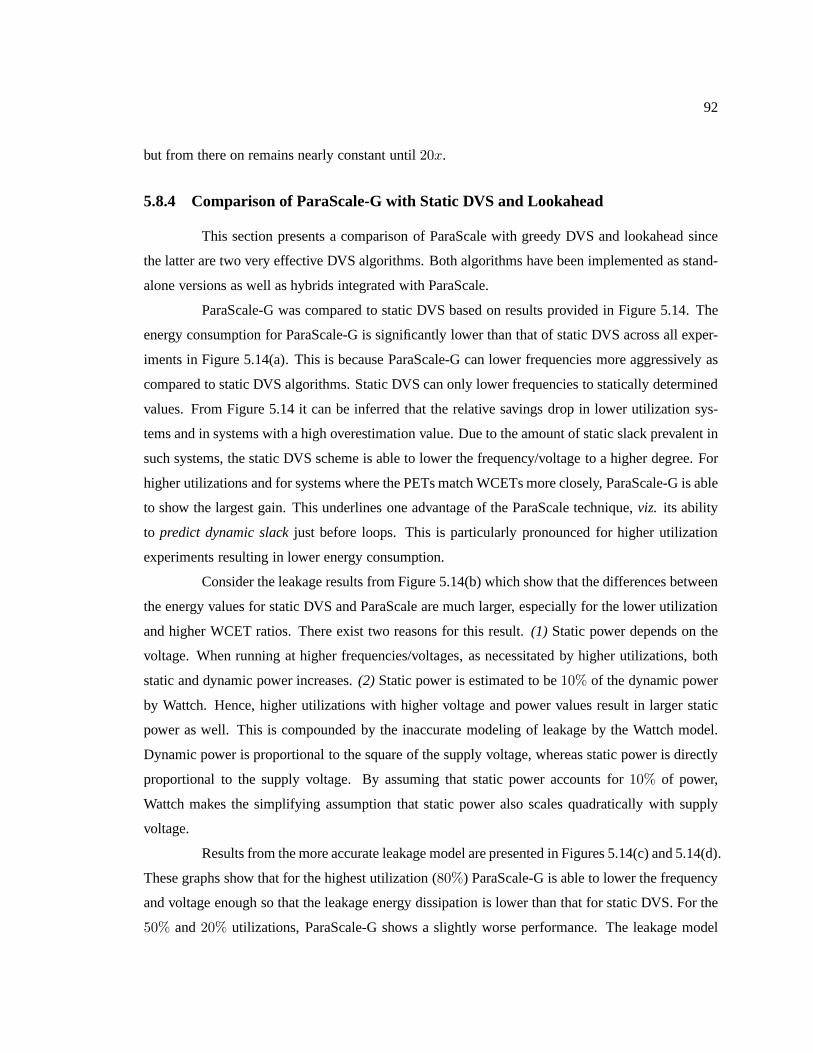
92

but from there on remains nearly constant until20x.

5.8.4 Comparison of ParaScale-G with Static DVS and Lookahead

This section presents a comparison of ParaScale with greedyDVS and lookahead since

the latter are two very effective DVS algorithms. Both algorithms have been implemented as stand-

alone versions as well as hybrids integrated with ParaScale.

ParaScale-G was compared to static DVS based on results provided in Figure 5.14. The

energy consumption for ParaScale-G is significantly lower than that of static DVS across all exper-

iments in Figure 5.14(a). This is because ParaScale-G can lower frequencies more aggressively as

compared to static DVS algorithms. Static DVS can only lowerfrequencies to statically determined

values. From Figure 5.14 it can be inferred that the relativesavings drop in lower utilization sys-

tems and in systems with a high overestimation value. Due to the amount of static slack prevalent in

such systems, the static DVS scheme is able to lower the frequency/voltage to a higher degree. For

higher utilizations and for systems where the PETs match WCETs more closely, ParaScale-G is able

to show the largest gain. This underlines one advantage of the ParaScale technique,viz. its ability

to predict dynamic slackjust before loops. This is particularly pronounced for higher utilization

experiments resulting in lower energy consumption.

Consider the leakage results from Figure 5.14(b) which showthat the differences between

the energy values for static DVS and ParaScale are much larger, especially for the lower utilization

and higher WCET ratios. There exist two reasons for this result. (1) Static power depends on the

voltage. When running at higher frequencies/voltages, as necessitated by higher utilizations, both

static and dynamic power increases.(2) Static power is estimated to be10% of the dynamic power

by Wattch. Hence, higher utilizations with higher voltage and power values result in larger static

power as well. This is compounded by the inaccurate modelingof leakage by the Wattch model.

Dynamic power is proportional to the square of the supply voltage, whereas static power is directly

proportional to the supply voltage. By assuming that staticpower accounts for10% of power,

Wattch makes the simplifying assumption that static power also scales quadratically with supply

voltage.

Results from the more accurate leakage model are presented in Figures 5.14(c) and 5.14(d).

These graphs show that for the highest utilization (80%) ParaScale-G is able to lower the frequency

and voltage enough so that the leakage energy dissipation islower than that for static DVS. For the

50% and20% utilizations, ParaScale-G shows a slightly worse performance. The leakage model

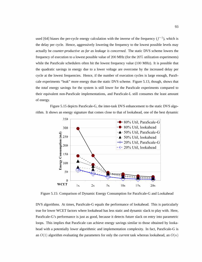
93

used [64] biases the per-cycle energy calculation with the inverse of the frequency (f−1), which is

the delay per cycle. Hence, aggressively lowering the frequency to the lowest possible levels may

actually becounter-productive as far as leakage is concerned. The static DVS scheme lowers the

frequency of execution to a lowest possible value of200 MHz (for the20% utilization experiments)

while the ParaScale schedulers often hit the lowest frequency value (100 MHz). It is possible that

the quadratic savings in energy due to a lower voltage are overcome by the increased delay per

cycle at the lowest frequencies. Hence, if the number of execution cycles is large enough, ParaS-

cale experiments “leak” more energy than the static DVS scheme. Figure 5.13, though, shows that

the total energy savings for the system is still lower for the ParaScale experiments compared to

their equivalent non-ParaScale implementations, and ParaScale-L still consumes the least amount

of energy.

Figure 5.15 depicts ParaScale-G, the inter-task DVS enhancement to the static DVS algo-

rithm. It shows an energy signature that comes close to that of lookahead, one of the best dynamic

���������������������

������������������Figure 5.15: Comparison of Dynamic Energy Consumption for ParaScale-G and Lookahead

DVS algorithms. At times, ParaScale-G equals the performance of lookahead. This is particularly

true for lower WCET factors where lookahead has less static and dynamic slack to play with. Here,

ParaScale-G’s performance is just as good, because it detects future slack on entry into parametric

loops. This implies that ParaScale can achieve energy savings similar to those obtained by looka-

head with a potentially lower algorithmic and implementation complexity. In fact, ParaScale-G is

anO(1) algorithm evaluating the parameters for only thecurrent task whereas lookahead, anO(n)

94

algorithm traversing through all tasks in the system. This becomes more relevant as the number of

tasks in the system is increased.

5.8.5 Overheads

The overheads imposed by the scheduler (especially the parametric scheduler, due to mul-

tiple calls made to it during task execution) and the frequency/voltage switching overheads are side-

effects of the ParaScale technique. These scheduler overheads impose additional execution time on

the system. The scheduler overheads were modeled using the timing analysis framework and are

enumerated in Table 5.3. When compared to the execution cycles for the tasks (Table 5.4) in the sys-

tem, the scheduler overheads are almost negligible. For example, the largest number of cycles used

during a scheduler invocation is for the inter-task lookahead scheduler (8627 cycles). This value is

less than0.8% of the WCEC for the smallest task in the system,viz. LMS. Hence, the scheduler

overheads have no significant impact on the execution of the tasks or the amount of energy savings.

Frequency Switch Overheads

To study the overheads imposed by the switching of frequencies and voltages, we imposed

the overhead for a synchronous switch observed on an IBM PowerPC 405LP [139]. The actual value

used was162µs for the overhead.Data was collected on the number of frequency/voltage transitions

for each experiment. The exact value of switching overhead varies depending on the actual differ-

ence between the voltages and whether it is being increased or decreased. This pessimistic, worst-

case value was used to measure the worst possible switching overhead for the system. The highest

overhead is incurred for the20x overestimation case with utilization of80% for ParaScale-G. The

cumulative value for the overhead in this case was42ms. To put this in perspective, assume that

the entire simulation had executed at the maximum frequencyof 1 GHz. (thus completing in the

shortest possible duration). The hyperperiod for each experiment was1.2 seconds. All experiments

were designed to execute forone hyperperiods. Since the tasksets execute at lower frequencies than

the maximum, they will take longer to complete but still finish within their deadlines. Also, the fre-

quency switch overhead is typically lower than162µs (depending on the exact difference between

the voltage/frequency levels). Hence, it is safe to assume that the frequency switch overheads would

bemuchless than the worst-case value of42ms. Typically, the overheads would be close to, or even

less than,1% of the total execution time of all tasks.

The energy consumption for the time period when the switching is taking place (162µs)

95

was also measured, for all three energy schemes – PCG, PCGL and PCGL-W. The respective values

were0.493 mJ,0.007 mJ and0.732 mJ, respectively, at1 GHz. Considering the energy signature

of the entire task set and the experiments, it is possible to conclude that the energy overheads for

frequency switching will be negligible.

5.9 Conclusion

This chapter details:

1. the development of a novel technique of parametric timinganalysis that obtains a formula to

express WCET bounds, which is subsequently integrated intothe code of tasks

2. the derivation of techniques to exploit parametric formulaevia online scheduling and power-

aware scheduling.

Parametric formulae are integrated into the timing analysis process without sacrificing the

tightness of WCET bounds. A fixed point approach to embed parametric formulae into application

code is derived, which bounds the WCET of not only the application code but also the embedded

parametric functions and their calls once integrated into the application. Prior to entering paramet-

ric loops, the actual loop bounds are discovered and then used to provide WCET bounds for the

remainder of execution of the tasks that are tighter than their static counterpart.

The benefit from parametric analysis is quantified in terms ofpower savings for sole

intra-task DVS as well asParaScale-G, the combined intra-task and greedy inter-task DVS. Pro-

cessor frequency and voltage are scaled down as loop bounds of parametric loops are discovered.

Power savings ranging between66% to 80% compared to DVS-oblivious techniques are observed,

depending on system utilization and the amount of overestimation for loop bounds. These energy

savings are comparable to other DVS algorithms based on dynamic priority scheduling. Yet, the

intra-task scheme (ParaScale) incurs a lower time complexity and can be implemented as an exten-

sion tostatic priority schedulingor cyclic executives. Conventional timing analysis methods will

be unable to achieve these benefits due to the lack of knowledge about remaining execution times

of tasks in conventional static timing analysis. This illustrates the potential impact of PTA on the

filed of timing analysis and real-time systems practitioners.

Overall, parametric timing analysis expands the class of applications for real-time systems

to programs with dynamic loop bounds that are loop invariantwhile retaining tight WCET bounds

and uncovering additional slack in the schedule.

96

Chapter 6

Temporal Analysis for Adapting

Concurrent Applications to Embedded

Systems1

6.1 Summary

Embedded services and applications that interact with the real world often, over time,

need to run on different hardware (low-cost microcontrollers to powerful multicore processors). It

is difficult to write one program that would work reliably on such a wide range of devices. This is

especially true when the application must be temporally predictable and robust, which is usually the

case since the physical world works in real-time.

This chapter introduces a representation of the temporal behavior of distributed real-time

applications as colored graphs that capture the timing of temporally continuous sections of execution

and dependencies between them, thereby creating a partial order. A method of extracting the graph

from existing applications is introduced through a combination of analysis techniques. Once the

graph has been created, a number of graph transformations are carried out to extract “meaning”

from the graph. The knowledge thus gained can be utilized forscheduling and for adjusting the

level of parallelism suitable to the specific hardware, for identifying hot spots, false parallelism, or

even candidates for additional concurrency.

The importance of these contributions is evident when such graphs can be sequentialized

1This is collaborative work with Johannes Helander that the author conducted during an internship at MicrosoftResearch in Summer 2007.

97

and can then be used as input for offline, online, or even distributed real-time scheduling. Results

from analysis of a complete TCP/IP stack and smaller test applications are presented to show that

the use of different analysis models result in a reduction ofthe complexity of the graphs. An im-

portant outcome is that increasing the expression of concurrency can reduce the level of parallelism

required, thus saving memory on deeply embedded platforms while keeping the program paralleliz-

able whenever complete serializability is not required. Applications that were previously considered

to be too complex for characterization of their worst-case behavior are now analyzable due to the

combination of analysis techniques presented here.

6.2 Introduction

Previous chapters introduced analysis techniques to deal with hardware complexity (Chap-

ters 2, 3, 4) andsomecomplexities in software (Chapter 5). While the latter was able to im-

prove analysis techniques for some types of embedded software, it still dealt with relatively simple,

straight-line,single-threadedcode. It did not deal with situations where embedded systemsneed to

be distributed in nature withmultiple threadsof execution. This chapter aims to analyze such com-

plex pieces of software. We are increasingly depending on such systems in our everyday lives in

health care, robotics, infrastructure, entertainment andeven clothing. Such applications and other

cyber-physical systems run on different embedded hardwareplatforms ranging from 8-bit micro-

controllers to sophisticated multicores. Since we depend on these devices, they must be robust and

as they interact with the real world, they must work in real time. Hence, their temporal behavior

must be robust and predictable. Unfortunately, it is quite difficult to write one program that would

work reliably on such a wide range of devices. This is particularly difficult if timing depends not

only on the application, but also on hardware details and other applications on the device. This

makes application development slow and expensive.

6.2.1 Awareness of Hardware Capabilities

It is important to pay attention to the hardware capabilities of a given target platform, such

as the number of processors and amount of available memory. In a low-cost microcontroller the

scarcest resource is often memory, and in particular physical RAM. Early experience with service-

oriented cyber-physical systems [55] shows that one of biggest RAM users tend to be thread stacks.

Note: this represents actual,physical memorysince such embedded systems do not have memory

98

management units or virtual memory. They also require that each thread be allocated the largest

possible, worst-case memory for stack space. This is true even for non real-time systems, because

running out of stack space can be catastrophic as the thread will crash and potentially take down the

entire system. Hence, solutions aim at reducing the number of threads. This implies that the amount

of parallelism needs to be reduced– i.e., the application needs to be executed sequentially.

In contrast, on a high-end multicore processor the bottleneck is not memory but the

amount of parallelism available in the application. It often makes sense to execute the same ser-

vice application on both ends of the embedded spectrum with only the throughput and the number

of services being varied. Thus, the applications need to be tuned in such a way as to address the

bottlenecks on each platform – the application needs to besequentialized for the low-end platform

andparallelized for the high-end platform. To this end, thefuture, a delayed function call (originally

proposed for handling synchronization in MultiLisp [47] and later used in other languages), is used

as a way of expressinglight-weight potential parallelism.

6.2.2 Model-based Development

Having a model that would enable

1. analysis of the program’s temporal behavior and

2. provide the ability to match it to a given hardware

would be most helpful. Helanderet al. [57] showed how new programs could be written together

using such a model. The model can be represented and manipulated as a graph, as discussed in this

chapter, or serialized to XML as shown by the authors of that paper. The serialized version of the

model is called “partiture”, an expression analogous to a short score in music where theconductor

can see what instruments should play at a given time without regard to the details of how they do it.

In practice though, most pre-existing applications do not follow model-based development

practices, but it is still desirable to adapt them to new platforms. This even applies to large software

projects in general where few, if any, engineers understandhow a program actually behaves due to

large development teams and changes over product revisions. Helping engineers understand and

modify complex software would be useful. This chapter proposes an automated process whereby

existing applications can be transferred to usepartitures and futures [57] to make model-based

scaling possible while maintaining correct program execution. This would reduce the tedious and

99

error prone methods for transforming applications by hand when they need to be deployed on new

platforms.

A tool thatextracts temporal models from existing applicationsis introduced in this chap-

ter. The knowledge gained can help designers of such systemsin:

1. optimization of programs fordifferent platforms,

2. distributed orchestration,

3. adaptation andscheduling[57,102], and

4. execution on modeling engines [62] to check forcorrectness.

6.2.3 Limitations of Analysis Techniques

Knowledge of the temporal behavior of an application is hidden inside the application

logic where it is extremely difficult to analyze and model forany given hardware. While static and

dynamic timing analyses are used to obtain the worst-case execution times (WCETs) for real-time

applications, they may not able to provide a complete picture of a program. This is particularly

true in the case of larger, more complex programs. Programs that contain function pointers are

typically out of the reach of static analyzers. Dynamic analyzers are unable to gauge the true nature

of the program and have shown to be unsafe [126] –i.e., they may underestimate the WCET of the

program, which could lead to dangerous effects. If the application usesconcurrency constructssuch

as signals, locks or mutexes, thenneitherof these techniques can fully analyze the application.

6.2.4 Contributions

This chapter presents the use of a combination of a variety oftechniques to form the com-

plete picture of the structure and execution characteristics of adistributed embedded application.

The collected information is used to createtiming graphs. The timing graph and thepartiture are

two representations of the same information. The nodes in the timing graph could represent simple

code sections (e.g. basic blocks) or complex structures (e,g,groups of functions), all combined

into temporal phases. The edges in the graph represent transitions between the phases, both be-

tween phases within the same thread as well as interactions between threads. Abar corresponds

to a node in the graph. Triggers and sequences between the bars correspond to the graph edges.

This means that the graph can simply be converted to a partiture and then be used for purposes such

100

as inputs for offline, online, or distributed real-time scheduling or potentially even converted to a

model program [57].

Finally, results are presented from a prototype analyzer that was used on a complete

TCP/IP stackin addition to smaller test applications. Perhaps the most interesting and surprising

result is thatincreasing the expression of concurrency can reduce the level of parallelism required

and save memory on deeply embedded platforms. Hence, the main contributions of this chapter are:

1. To extend the scope of static (and dynamic) timing analysis to more complex applications by

combining it with other techniques, in particular run-timetraces and type inference. Applica-

tions that were previously considered to be “un-analyzable” due to their inherent complexity

are now analyzed using the graph capture and transformationtechniques – their worst-case

behavior can now be characterized correctly.

2. To define a colored graph representation of a program’s temporal behavior, including invari-

ants and transformations. The graph corresponds to apartiture, a programmatic expression.

Transitively, it also corresponds to a model program that can be executed on a modeling tool.

3. To derive information from the topology of graphs, thus allowing an engineer to optimize

an application such as to make it more scalable and amenable to being transformed into the

application model presented here (partitures, futures,etc.). Some such knowledge that can be

gleaned – the minimum number of threads required for an application to correctly execute,

graph sections with potential false parallelism, and dependencies that prevent parallelization.

4. To observe that adding concurrency can save memory and present methods to an engineer to

pinpoint areas where concurrency can be increased.

5. To allow an engineer to learn something about the application behavior and augment the

automatically generated model with manually provided domain knowledge. Due to the incre-

mental nature of the analysis, even an incompletely understood application can be explored.

This is a critical step forward as embedded designers now have more choices in the type of

applications that they can develop, especially for time-constrained systems.

6. To demonstrate that creating the timing graph and performing subsequent transformations

is feasible by means of presenting an implementation that was applied to actual embedded

software – the TCP/IP stack of an embedded operating system.

101

One important feature of the techniques presented in this chapter is that they areindepen-

dent of the programming languageused.

The use of the combination of analysis techniques presentedin this chapter enables the

process of extracting temporal behavior from existing applications. This ultimately leads to the

development of distributed embedded applications on varied platforms. Such analysis is the first of

its kind.

The rest of this chapter is organized as follows: The use offuturesin embedded software

is discussed in Section 6.3. The colored graph representinga program’s temporal behavior is intro-

duced in Section 6.4, together with invariants that define a valid graph. The algorithm for creating

temporal graphs is introduced in Section 6.5. Transformations that can be used to simplify and/or

reveal interesting topological properties of the graph aredefined in Section 6.6. Section 6.7 explains

insights obtained from the graph transformations. Section6.8 details the experimental framework

and methods to collect the raw data required for graph generation. Section 6.9 presents the results

followed by the conclusion being presented in Section 6.10.

6.3 Saving Memory through Sequential Execution

In low-end microcontrollers a multi-threaded applicationuses one stack for each thread.

Since microcontrollers do not usually have a memory management unit, each thread stack must be

allocated from physical memory. The maximum size of the stack is limited by the available memory

The minimum is the largest stack the thread may ever need. Once a thread has been created it cannot

give up its stack, whether running or blocked, since there are live stack frames occupying part of

the stack. This is the case even before the thread has run for the first time as an initial stack frame

must be created by the runtime. The stacks cannot be moved as frames in it contain pointers to

data in other stack frames and cannot be compacted as executing code may need to push additional

frames. As a final option, copying, compressing, and decompressing stacks at each context switch

to the side and sharing the actual stack between threads would be complex and inefficient. Clearly,

threads are problematic on low-end embedded systems.

The most common alternative is an event loop. Instead of creating a thread to handle

a sensor reading, for instance, an event is posted. A loop in the program then picks up an event

and examines it. The disadvantages to this are –(1) all applications turn into state machines with

complex interactions. Thus, the code becomes hard to understand. (2) The development process

becomes error prone with skyrocketing maintenance costs.

102

One approach is to transform an application written with threads to use the so-called split-

phase operation [4] where the temporal phases of a thread aresplit into separate functions. However,

no automated transformation from existing programs has been available because significant engi-

neering effort is required for carrying out such a transformation. The approach has been codified in

the NesC programming language [40]. Unfortunately the split-phase mode is essentially the same

as an event-driven model, including the need to communicatestate from one phase to another in

global variables or objects pointed to by global variables.

One attempt at combining the features of thread-based programming and event handling

is protothreads [32] where stacks are unwound at blocking points. While this appears to work only

in the C programming language, the implementation relies onnon-standard features in a specific

compiler (which it uses in a clever way). More importantly, protothreads do not save local variables

during blocks, making the appearance of thread programmingat best an appearance and at worst an

endless source of difficult bugs.

6.3.1 Futures

Futures[37] were originally proposed in the Lisp community as a way of deferring evalu-

ation and increasing performance [39]. They were used as a primary construct for concurrency and

synchronization in MultiLisp [47]. Futures have also been implemented in mid-level languages,

such as Java [31] or C#. Futures have been natively implemented in C on a microcontroller in ear-

lier work [57]. When C programs are written in an object-oriented fashion, it is easy to turn any

method call into a future with few modifications to the program. Threads can also be converted

to futures. Creating a future is similar to calling a method or function, yet the call is executed

asynchronously. Parameters are delivered like regular function calls. If a split-phase program was

rewritten in terms of futures, its phases could send values to the following phase in normal function

parameters, includingthis pointers in object-oriented programs, thus obviating the use of global

variables, an engineering practice commonly advocated in the last few decades. Compared to pro-

tothreads, the normal language rules are in effect and asynchrony is explicit and controlled.

Instead of being implied or encoded in the program, such as intraditional threads pro-

gramming, timing parameters and any required concurrent execution is expressed in a partiture

where each future is associated with one or more bars. The advantage of futures over threads is that

futures can be inserted anywhere (there isno predetermined parallelism, only concurrency), stack

allocation can be deferred until the future is ready to run, and the cost of creating a creating a future

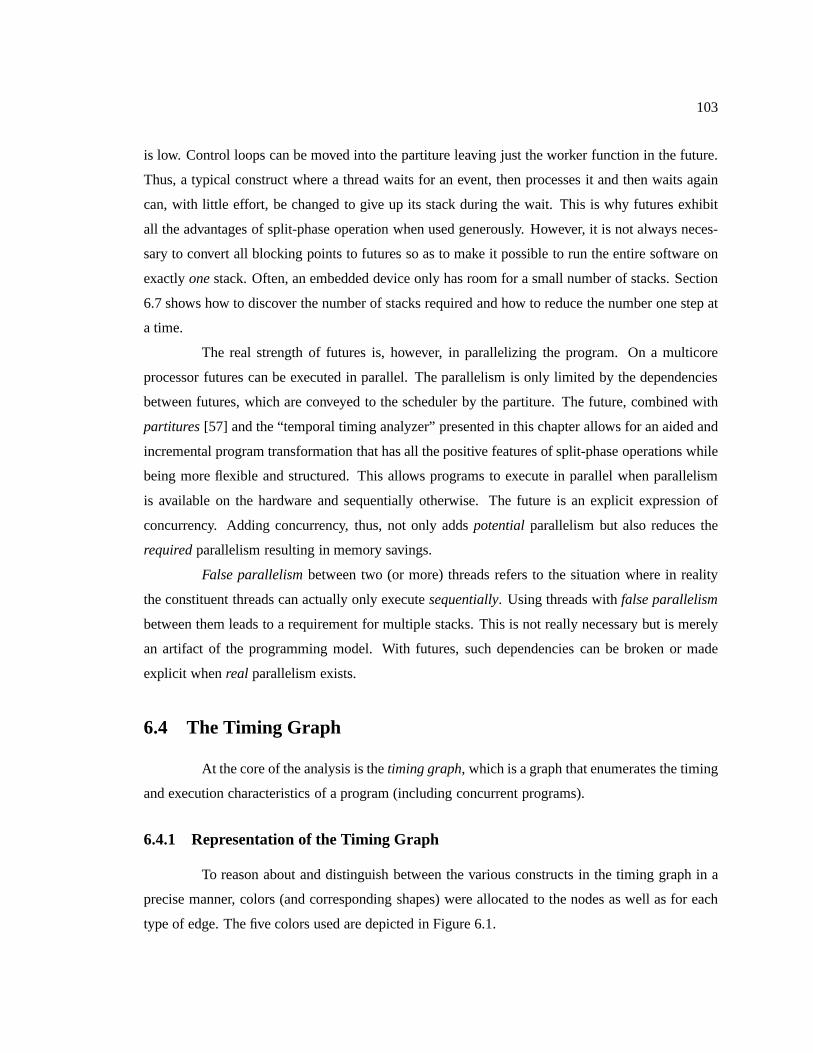
103

is low. Control loops can be moved into the partiture leavingjust the worker function in the future.

Thus, a typical construct where a thread waits for an event, then processes it and then waits again

can, with little effort, be changed to give up its stack during the wait. This is why futures exhibit

all the advantages of split-phase operation when used generously. However, it is not always neces-

sary to convert all blocking points to futures so as to make itpossible to run the entire software on

exactlyonestack. Often, an embedded device only has room for a small number of stacks. Section

6.7 shows how to discover the number of stacks required and how to reduce the number one step at

a time.

The real strength of futures is, however, in parallelizing the program. On a multicore

processor futures can be executed in parallel. The parallelism is only limited by the dependencies

between futures, which are conveyed to the scheduler by the partiture. The future, combined with

partitures[57] and the “temporal timing analyzer” presented in this chapter allows for an aided and

incremental program transformation that has all the positive features of split-phase operations while

being more flexible and structured. This allows programs to execute in parallel when parallelism

is available on the hardware and sequentially otherwise. The future is an explicit expression of

concurrency. Adding concurrency, thus, not only addspotential parallelism but also reduces the

requiredparallelism resulting in memory savings.

False parallelismbetween two (or more) threads refers to the situation where in reality

the constituent threads can actually only executesequentially. Using threads withfalse parallelism

between them leads to a requirement for multiple stacks. This is not really necessary but is merely

an artifact of the programming model. With futures, such dependencies can be broken or made

explicit whenreal parallelism exists.

6.4 The Timing Graph

At the core of the analysis is thetiming graph, which is a graph that enumerates the timing

and execution characteristics of a program (including concurrent programs).

6.4.1 Representation of the Timing Graph

To reason about and distinguish between the various constructs in the timing graph in a

precise manner, colors (and corresponding shapes) were allocated to the nodes as well as for each

type of edge. The five colors used are depicted in Figure 6.1.

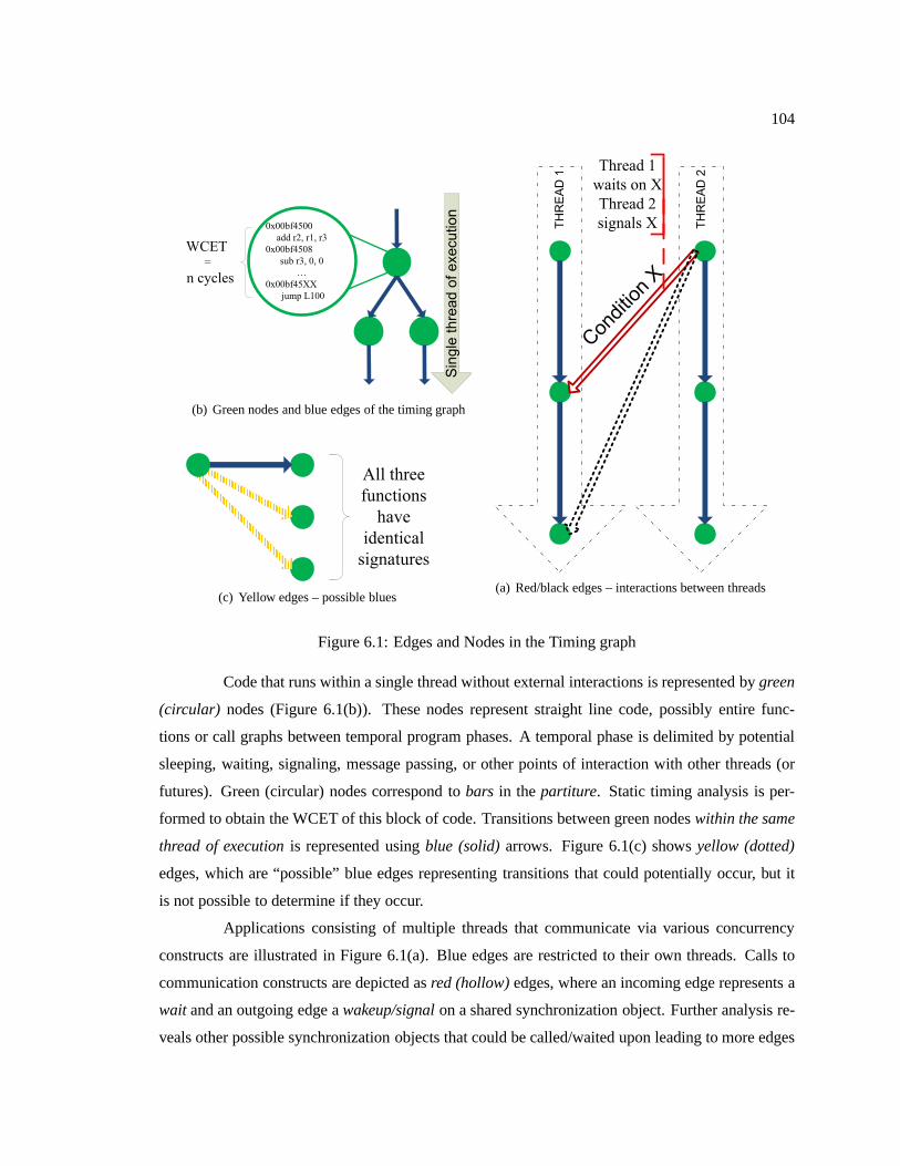
104

(a) Red/black edges – interactions between threads

(b) Green nodes and blue edges of the timing graph

(c) Yellow edges – possible blues

Figure 6.1: Edges and Nodes in the Timing graph

Code that runs within a single thread without external interactions is represented bygreen

(circular) nodes (Figure 6.1(b)). These nodes represent straight linecode, possibly entire func-

tions or call graphs between temporal program phases. A temporal phase is delimited by potential

sleeping, waiting, signaling, message passing, or other points of interaction with other threads (or

futures). Green (circular) nodes correspond tobars in thepartiture. Static timing analysis is per-

formed to obtain the WCET of this block of code. Transitions between green nodeswithin the same

thread of executionis represented usingblue (solid)arrows. Figure 6.1(c) showsyellow (dotted)

edges, which are “possible” blue edges representing transitions that could potentially occur, but it

is not possible to determine if they occur.

Applications consisting of multiple threads that communicate via various concurrency

constructs are illustrated in Figure 6.1(a). Blue edges arerestricted to their own threads. Calls to

communication constructs are depicted asred (hollow)edges, where an incoming edge represents a

wait and an outgoing edge awakeup/signalon a shared synchronization object. Further analysis re-

veals other possible synchronization objects that could becalled/waited upon leading to more edges

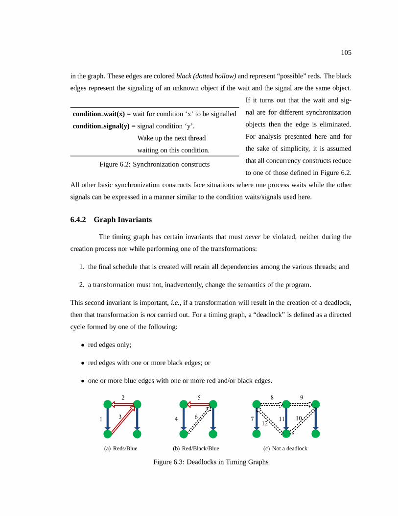
105

in the graph. These edges are coloredblack (dotted hollow)and represent “possible” reds. The black

edges represent the signaling of an unknown object if the wait and the signal are the same object.

condition wait(x) = wait for condition ‘x’ to be signalled

condition signal(y) = signal condition ‘y’.

Wake up the next thread

waiting on this condition.

Figure 6.2: Synchronization constructs

If it turns out that the wait and sig-

nal are for different synchronization

objects then the edge is eliminated.

For analysis presented here and for

the sake of simplicity, it is assumed

that all concurrency constructs reduce

to one of those defined in Figure 6.2.

All other basic synchronization constructs face situations where one process waits while the other

signals can be expressed in a manner similar to the conditionwaits/signals used here.

6.4.2 Graph Invariants

The timing graph has certain invariants that mustneverbe violated, neither during the

creation process nor while performing one of the transformations:

1. the final schedule that is created will retain all dependencies among the various threads; and

2. a transformation must not, inadvertently, change the semantics of the program.

This second invariant is important,i.e., if a transformation will result in the creation of a deadlock,

then that transformation isnotcarried out. For a timing graph, a “deadlock” is defined as a directed

cycle formed by one of the following:

• red edges only;

• red edges with one or more black edges; or

• one or more blue edges with one or more red and/or black edges.

(a) Reds/Blue (b) Red/Black/Blue (c) Not a deadlock

Figure 6.3: Deadlocks in Timing Graphs

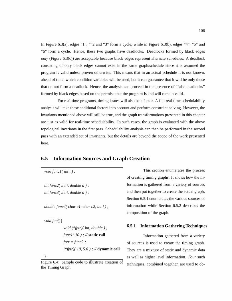
106

In Figure 6.3(a), edges “1”, “”2 and “3” form a cycle, while inFigure 6.3(b), edges “4”, “5” and

“6” form a cycle. Hence, these two graphs have deadlocks. Deadlocks formed by black edges

only (Figure 6.3(c)) are acceptable because black edges represent alternate schedules. A deadlock

consisting of only black edges cannot exist in the same graph/schedule since it is assumed the

program is valid unless proven otherwise. This means that inan actual schedule it is not known,

ahead of time, which condition variables will be used, but itcan guarantee that it will be only those

that do not form a deadlock. Hence, the analysis can proceed in the presence of “false deadlocks”

formed by black edges based on the premise that the program isand will remain valid.

For real-time programs, timing issues will also be a factor.A full real-time schedulability

analysis will take these additional factors into account and perform constraint solving. However, the

invariants mentioned above will still be true, and the graphtransformations presented in this chapter

are just as valid for real-time schedulability. In such cases, the graph is evaluated with the above

topological invariants in the first pass. Schedulability analysis can then be performed in the second

pass with an extended set of invariants, but the details are beyond the scope of the work presented

here.

6.5 Information Sources and Graph Creation

void func1( int i ) ;

int func2( int i, double d ) ;

int func3( int i, double d ) ;

double func4( char c1, char c2, int i ) ;

void foo(){

void (*fptr)( int, double ) ;

func1( 10 ) ; //static call

fptr = func2 ;

(*fptr)( 10, 5.0 ) ; //dynamic call

}

Figure 6.4: Sample code to illustrate creation ofthe Timing Graph

This section enumerates the process

of creating timing graphs. It shows how the in-

formation is gathered from a variety of sources

and then put together to create the actual graph.

Section 6.5.1 enumerates the various sources of

information while Section 6.5.2 describes the

composition of the graph.

6.5.1 Information Gathering Techniques

Information gathered from a variety

of sources is used to create the timing graph.

They are a mixture of static and dynamic data

as well as higher level information.Four such

techniques, combined together, are used to ob-

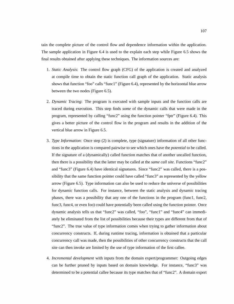
107

tain the complete picture of the control flow and dependence information within the application.

The sample application in Figure 6.4 is used to the explain each step while Figure 6.5 shows the

final results obtained after applying these techniques. Theinformation sources are:

1. Static Analysis: The control flow graph (CFG) of the application is created and analyzed

at compile time to obtain the static function call graph of the application. Static analysis

shows that function “foo” calls “func1” (Figure 6.4), represented by the horizontal blue arrow

between the two nodes (Figure 6.5).

2. Dynamic Tracing: The program is executed with sample inputs and the functioncalls are

traced during execution. This step findssomeof the dynamic calls that were made in the

program, represented by calling “func2” using the functionpointer “fptr” (Figure 6.4). This

gives a better picture of the control flow in the program and results in the addition of the

vertical blue arrow in Figure 6.5.

3. Type Information: Once step (2) is complete, type (signature) information ofall other func-

tions in the application is compared pairwise to see which ones have thepotentialto be called.

If the signature of a (dynamically) called function matchesthat of another uncalled function,

then there is a possibility that the latter may be called at thesame call site. Functions “func2”

and “func3” (Figure 6.4) have identical signatures. Since “func2” was called, there is a pos-

sibility that the same function pointer could have called “func3” as represented by the yellow

arrow (Figure 6.5). Type information can also be used to reduce the universe of possibilities

for dynamic function calls. For instance, between the static analysis and dynamic tracing

phases, there was a possibility that any one of the functionsin the program (func1, func2,

func3, func4, or even foo) could have potentially been called using the function pointer. Once

dynamic analysis tells us that “func2” was called, “foo”, “func1” and “func4” can immedi-

ately be eliminated from the list of possibilities because their types are different from that of

“func2”. The true value of type information comes when trying to gather information about

concurrency constructs. If, during runtime tracing, information is obtained that a particular

concurrency call was made, then the possibilities of other concurrency constructs that the call

site can then invoke are limited by the use of type information of the first callee.

4. Incremental developmentwith inputs from the domain expert/programmer: Outgoing edges

can be further pruned by inputs based on domain knowledge. For instance, “func3” was

determined to be a potential callee because its type matchesthat of “func2”. A domain expert

108

might be able to point out that based on the application design there isnevera possibility that

both “func2” and “func3” are called during the same execution instance of the application.

This could be the case in a typical network stack where “tcpsend” and “udpsend” probably

have the same function signatures but can never be called from the same call site. Hence an

incremental development process that combines inputs fromthe automated techniques and

the programmer can improve the understanding of the application.

Figure 6.5: Timing graph created by ap-plication of various information gather-ing techniques

Further known techniques, such as abstract ex-

ecution, flow analysis,etc., as well as techniques that will

be developed in the future, can be used to gather more in-

formation and make the graph more complete. The anal-

ysis can remain the same and take advantage of a graph

that has more information. This will reduce the time for

the analysis and provide more accurate results.

6.5.2 Graph Creation

The timing graph is actually created in stages. The green nodes in the graph which repre-

sent straight-line execution within the same thread could be basic blocks in the CFG or even single

(or groups of) functions (at a higher level). Traditional static timing analysis is performed to obtain

the worst-case execution time (WCET) for this block of code.Edges obtained from static analysis as

well as those obtained from the dynamic traces form the blue arrows, which are added next. Yellow

edges are gleaned from type information and are then added tothe graph. Red edges are a result

of dynamic tracing where calls to concurrency constructs are also traced. Further type analysis re-

veals other possible conditions that could be called/waited upon, based on the type signature of the

previous callee, leading to black edges being inserted intothe graph.

Before the analysis is started, the number of “possible” edges in the function call graph

is large,i.e., any function can call any other function or signal/wait on any condition variable. With

static analysis, some of the yellow edges are turned into blue edges while some of the black edges

are turned into reds. Also, since static analysis fixes one outgoing edge per call site, it also eliminates

other yellow/red edges from the same call site, thus reducing the universe of possibilities. Further

analysis (runtime tracing) turns more of the yellows into blues and blacks into reds. However, this

step does not reduce any edges, as there is no guarantee that each call site has only one outgoing

edge. In fact, as seen in the case of function pointers, each call site could call many potential callees.

109

Type information, on the other hand, can prune some edges. Itrestricts possible outgoing edges

based on the type signature to blue and red edges that have been discovered during runtime analysis.

Hence, some yellow and black edges are removed from the graph. Finally, domain knowledge can

prune the graph further by removing impossible yellow and black edges from the graph. This multi-

colored, pruned graph is used for the analysis that follows in the next section.

6.6 Timing Graph Transformations

This section presents certain fixed graph transformations aimed at reducing the complex-

ity of these timing graphs. The transformations will also help the programmer find interesting topo-

logical and programmatic properties. As explained in Section 6.2, embedded systems have severe

resource constraints. Executing parallel code could lead to a high number of context switches and a

large number of threads, which ultimately leads to a high demand for stack space. Hence, reducing

the program to obtain theleastnumber of threads required for correct execution of the program aids

in reducing stack pressure. This also helps determine the limits of serializability of the program.

The transformation described in the remaining part of this section aids in achieving both of these

goals. The larger goals for performing these transformations are:

1. To find theminimumnumber of threads required for the application to function correctly;

2. To aid in understanding the program behavior/structure and help system designers to optimize

it. 2; and

3. To provide the ability toautomaticallygenerate partitures and, from them, the schedules of

execution on a particular system.

The timing graph and subsequent transformations could alsobe used, in the future, to achieve the

following goals:

• To aid in visualizing the program so that system designers could gain an understanding of the

true nature of the program;

• To aid in increasing the parallelism of the program by findingspots that are synchronization

bottlenecks,i.e., a concentration of edges in close vicinity;

2Specifically, this could find candidate spots for additionalconcurrency in the program, which makes the programmore scalable. It is also possible to find false parallelism in the program, wherein multiple threads must execute in aserial fashion for forward progress of the application

110

• To provide inputs for real-time schedulability analyzers and constraint solvers; and

• To aid in model-based testing of the application.

6.6.1 Assumptions

The transformations presented here rest on the following assumptions (or rather the pre-

conditions):

• A strict partial order is always maintained for the graph.

• The graph cannot have any deadlocks or race conditions (i.e., no unguarded resources). This

condition implies that the program must becorrect. Of course, benign races (such as bounded

atomic adds) are fine.

If the timing graph represents a real-time application, then certain additional constraints apply:

• Loop bounds must either be statically known or at least knownprior to loop entry.

• No code can be dynamically loaded,i.e., all modules in the application must be statically

known. This rule can be relaxed to state that all applications that could possibly be loaded

must be known. The system could then be treated as if everything had been preloaded. Of

course, this would introduce some pessimism into the analysis.

• The program must use afinite set of condition variables.

Note: The analyzer does not check for the correctness of programs but will axiomatically assume

the validity of programs and try to apply transformations.

6.6.2 Graph Pruning and Reduction

This section examines techniques used to reduce and simplify the graph. First,graph

pruning techniques are presented. They help in reducing “maybe” edges, either by transforming

them to actual, known edges (blue or red) or getting rid of them entirely. Section 6.4 already

introduced some methods for performing this pruning,e.g., dynamic traces prune some yellow

edges to blues,etc.Other techniques used are:

1. Black edges that result in “potential” deadlocks (with red or blue edges) are removed. The

program is assumed valid unless proven otherwise.

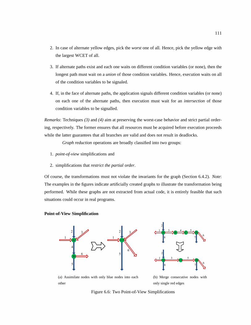
111

2. In case of alternate yellow edges, pick theworstone of all. Hence, pick the yellow edge with

the largest WCET of all.

3. If alternate paths exist and each one waits on different condition variables (or none), then the

longest path must wait on aunionof those condition variables. Hence, execution waits on all

of the condition variables to be signaled.

4. If, in the face of alternate paths, the application signals different condition variables (or none)

on each one of the alternate paths, then execution must wait for an intersectionof those

condition variables to be signalled.

Remarks: Techniques(3) and(4) aim at preserving the worst-case behavior and strict partial order-

ing, respectively. The former ensures that all resources must be acquired before execution proceeds

while the latter guarantees that all branches are valid and does not result in deadlocks.

Graph reductionoperations are broadly classified into two groups:

1. point-of-viewsimplifications and

2. simplifications thatrestrict the partial order.

Of course, the transformations must not violate the invariants for the graph (Section 6.4.2).Note:

The examples in the figures indicate artificially created graphs to illustrate the transformation being

performed. While these graphs are not extracted from actualcode, it is entirely feasible that such

situations could occur in real programs.

Point-of-View Simplification

(a) Assimilate nodes with only blue nodes into each

other

(b) Merge consecutive nodes with

only single red edges

Figure 6.6: Two Point-of-View Simplifications

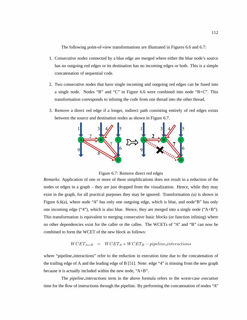
112

The following point-of-view transformations are illustrated in Figures 6.6 and 6.7:

1. Consecutive nodes connected by a blue edge are merged where either the blue node’s source

has no outgoing red edges or its destination has no incoming edges or both. This is a simple

concatenation of sequential code.

2. Two consecutive nodes that have single incoming and outgoing red edges can be fused into

a single node. Nodes “B” and “C” in Figure 6.6 were combined into node “B+C”. This

transformation corresponds to inlining the code from one thread into the other thread.

3. Remove a direct red edge if a longer, indirect path consisting entirely of red edges exists

between the source and destination nodes as shown in Figure 6.7.

Figure 6.7: Remove direct red edges

Remarks: Application of one or more of these simplifications does notresult in a reduction of the

nodes or edges in a graph – they are just dropped from the visualization. Hence, while they may

exist in the graph, for all practical purposes they may be ignored. Transformation(a) is shown in

Figure 6.6(a), where node “A” has only one outgoing edge, which is blue, and node“B” has only

one incoming edge (“4”), which is also blue. Hence, they are merged into a single node (“A+B”).

This transformation is equivalent to merging consecutive basic blocks (or function inlining) where

no other dependencies exist for the caller or the callee. TheWCETs of “A” and “B” can now be

combined to form the WCET of the new block as follows:

WCETA+B = WCETA + WCETB − pipeline interactions

where “pipelineinteractions” refer to the reduction in execution time due to the concatenation of

the trailing edge of A and the leading edge of B [51]. Note: edge “4” is missing from the new graph

because it is actually included within the new node, “A+B”.

The pipeline interactionsterm in the above formula refers to the worst-caseexecution

time for the flow of instructions through the pipeline. By performing the concatenation of nodes “A”

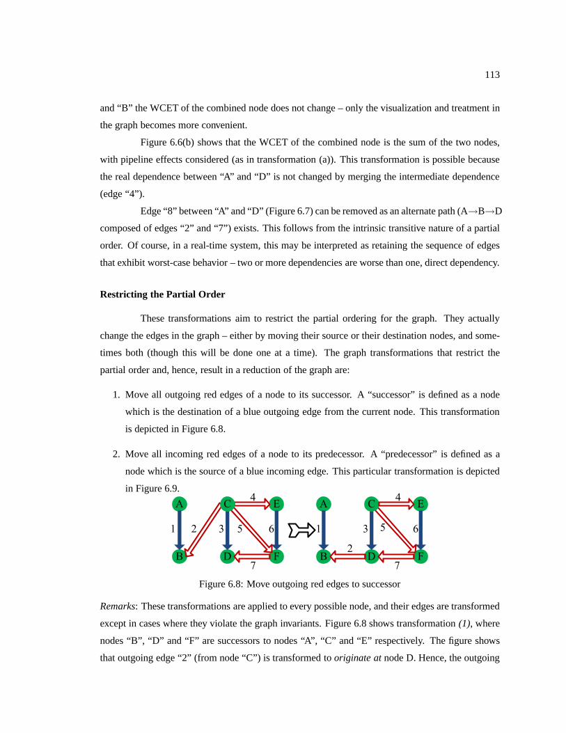
113

and “B” the WCET of the combined node does not change – only thevisualization and treatment in

the graph becomes more convenient.

Figure 6.6(b) shows that the WCET of the combined node is the sum of the two nodes,

with pipeline effects considered (as in transformation (a)). This transformation is possible because

the real dependence between “A” and “D” is not changed by merging the intermediate dependence

(edge “4”).

Edge “8” between “A” and “D” (Figure 6.7) can be removed as an alternate path (A→B→D

composed of edges “2” and “7”) exists. This follows from the intrinsic transitive nature of a partial

order. Of course, in a real-time system, this may be interpreted as retaining the sequence of edges

that exhibit worst-case behavior – two or more dependenciesare worse than one, direct dependency.

Restricting the Partial Order

These transformations aim to restrict the partial orderingfor the graph. They actually

change the edges in the graph – either by moving their source or their destination nodes, and some-

times both (though this will be done one at a time). The graph transformations that restrict the

partial order and, hence, result in a reduction of the graph are:

1. Move all outgoing red edges of a node to its successor. A “successor” is defined as a node

which is the destination of a blue outgoing edge from the current node. This transformation

is depicted in Figure 6.8.

2. Move all incoming red edges of a node to its predecessor. A “predecessor” is defined as a

node which is the source of a blue incoming edge. This particular transformation is depicted

in Figure 6.9.

Figure 6.8: Move outgoing red edges to successor

Remarks: These transformations are applied to every possible node,and their edges are transformed

except in cases where they violate the graph invariants. Figure 6.8 shows transformation(1), where

nodes “B”, “D” and “F” are successors to nodes “A”, “C” and “E”respectively. The figure shows

that outgoing edge “2” (from node “C”) is transformed tooriginate atnode D. Hence, the outgoing

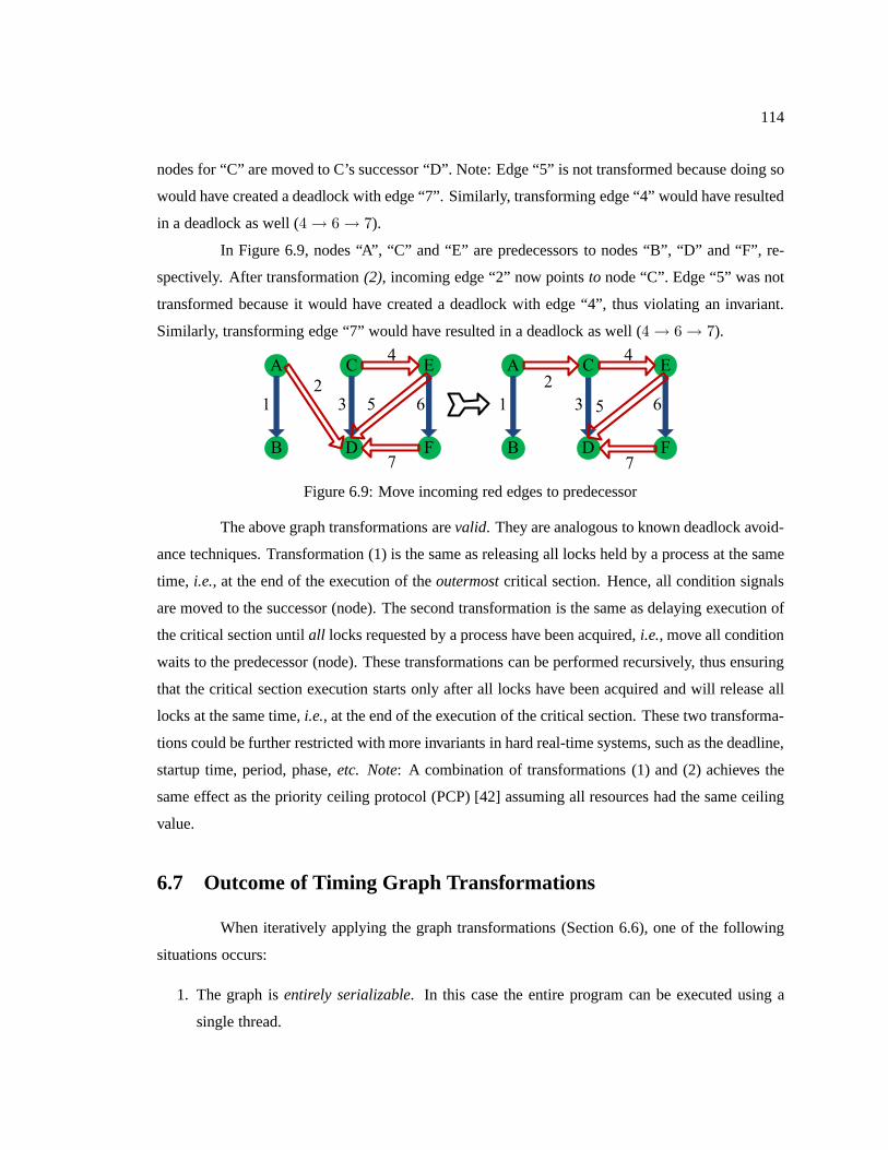
114

nodes for “C” are moved to C’s successor “D”. Note: Edge “5” isnot transformed because doing so

would have created a deadlock with edge “7”. Similarly, transforming edge “4” would have resulted

in a deadlock as well (4→ 6→ 7).

In Figure 6.9, nodes “A”, “C” and “E” are predecessors to nodes “B”, “D” and “F”, re-

spectively. After transformation(2), incoming edge “2” now pointsto node “C”. Edge “5” was not

transformed because it would have created a deadlock with edge “4”, thus violating an invariant.

Similarly, transforming edge “7” would have resulted in a deadlock as well (4→ 6→ 7).

Figure 6.9: Move incoming red edges to predecessor

The above graph transformations arevalid. They are analogous to known deadlock avoid-

ance techniques. Transformation (1) is the same as releasing all locks held by a process at the same

time, i.e., at the end of the execution of theoutermostcritical section. Hence, all condition signals

are moved to the successor (node). The second transformation is the same as delaying execution of

the critical section untilall locks requested by a process have been acquired,i.e., move all condition

waits to the predecessor (node). These transformations canbe performed recursively, thus ensuring

that the critical section execution starts only after all locks have been acquired and will release all

locks at the same time,i.e., at the end of the execution of the critical section. These two transforma-

tions could be further restricted with more invariants in hard real-time systems, such as the deadline,

startup time, period, phase,etc. Note: A combination of transformations (1) and (2) achieves the

same effect as the priority ceiling protocol (PCP) [42] assuming all resources had the same ceiling

value.

6.7 Outcome of Timing Graph Transformations

When iteratively applying the graph transformations (Section 6.6), one of the following

situations occurs:

1. The graph isentirely serializable. In this case the entire program can be executed using a

single thread.

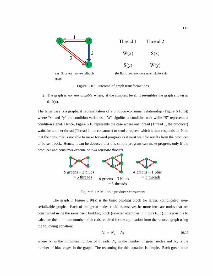
115

(a) Smallest non-serializable

graph

(b) Basic producer-consumer relationship

Figure 6.10: Outcome of graph transformations

2. The graph isnon-serializablewhere, at the simplest level, it resembles the graph shown in

6.10(a).

The latter case is a graphical representation of a producer-consumer relationship (Figure 6.10(b))

where “x” and “y” are condition variables. “W” signifies a condition wait while “S” represents a

condition signal. Hence, Figure 6.10 represents the case where one thread (Thread 1, the producer)

waits for another thread (Thread 2, the consumer) to send a request which it then responds to. Note

that the consumer is not able to make forward progress as it must wait for results from the producer

to be sent back. Hence, it can be deduced that this simple program can make progress only if the

producer and consumer execute ontwo separate threads.

Figure 6.11: Multiple producer-consumers

The graph in Figure 6.10(a) is the basic building block for larger, complicated, non-

serializable graphs. Each of the green nodes could themselves be more intricate nodes that are

constructed using the same basic building block (selected examples in Figure 6.11). It is possible to

calculate the minimum number of threads required for the application from the reduced graph using

the following equation:

Nt = Ng −Nb (6.1)

whereNt is the minimum number of threads,Ng is the number of green nodes andNb is the

number of blue edges in the graph. The reasoning for this equation is simple. Each green node

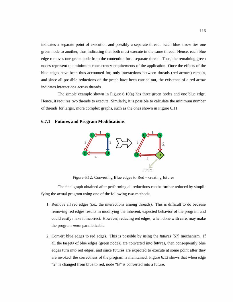
116

indicates a separate point of execution and possibly a separate thread. Each blue arrow ties one

green node to another, thus indicating that both must execute in the same thread. Hence, each blue

edge removes one green node from the contention for a separate thread. Thus, the remaining green

nodes represent the minimum concurrency requirements of the application. Once the effects of the

blue edges have been thus accounted for, only interactions between threads (red arrows) remain,

and since all possible reductions on the graph have been carried out, the existence of a red arrow

indicates interactions across threads.

The simple example shown in Figure 6.10(a) has three green nodes and one blue edge.

Hence, it requires two threads to execute. Similarly, it is possible to calculate the minimum number

of threads for larger, more complex graphs, such as the ones shown in Figure 6.11.

6.7.1 Futures and Program Modifications

Figure 6.12: Converting Blue edges to Red – creating futures

The final graph obtained after performing all reductions canbe further reduced by simpli-

fying the actual program using one of the following two methods:

1. Remove all red edges (i.e., the interactions among threads). This is difficult to do because

removing red edges results in modifying the inherent, expected behavior of the program and

could easily make it incorrect. However, reducing red edges, when done with care, may make

the programmoreparallelizable.

2. Convert blue edges to red edges. This is possible by using the futures[57] mechanism. If

all the targets of blue edges (green nodes) are converted into futures, then consequently blue

edges turn into red edges, and since futures are expected to execute at some point after they

are invoked, the correctness of the program is maintained. Figure 6.12 shows that when edge

“2” is changed from blue to red, node “B” is converted into a future.

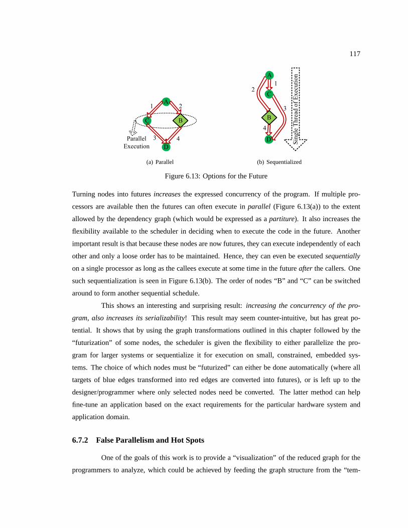
117

(a) Parallel (b) Sequentialized

Figure 6.13: Options for the Future

Turning nodes into futuresincreasesthe expressed concurrency of the program. If multiple pro-

cessors are available then the futures can often execute inparallel (Figure 6.13(a)) to the extent

allowed by the dependency graph (which would be expressed asa partiture). It also increases the

flexibility available to the scheduler in deciding when to execute the code in the future. Another

important result is that because these nodes are now futures, they can execute independently of each

other and only a loose order has to be maintained. Hence, theycan even be executedsequentially

on a single processor as long as the callees execute at some time in the futureafter the callers. One

such sequentialization is seen in Figure 6.13(b). The orderof nodes “B” and “C” can be switched

around to form another sequential schedule.

This shows an interesting and surprising result:increasing the concurrency of the pro-

gram, also increases its serializability! This result may seem counter-intuitive, but has great po-

tential. It shows that by using the graph transformations outlined in this chapter followed by the

“futurization” of some nodes, the scheduler is given the flexibility to either parallelize the pro-

gram for larger systems or sequentialize it for execution onsmall, constrained, embedded sys-

tems. The choice of which nodes must be “futurized” can either be done automatically (where all

targets of blue edges transformed into red edges are converted into futures), or is left up to the

designer/programmer where only selected nodes need be converted. The latter method can help

fine-tune an application based on the exact requirements forthe particular hardware system and

application domain.

6.7.2 False Parallelism and Hot Spots

One of the goals of this work is to provide a “visualization” of the reduced graph for the

programmers to analyze, which could be achieved by feeding the graph structure from the “tem-

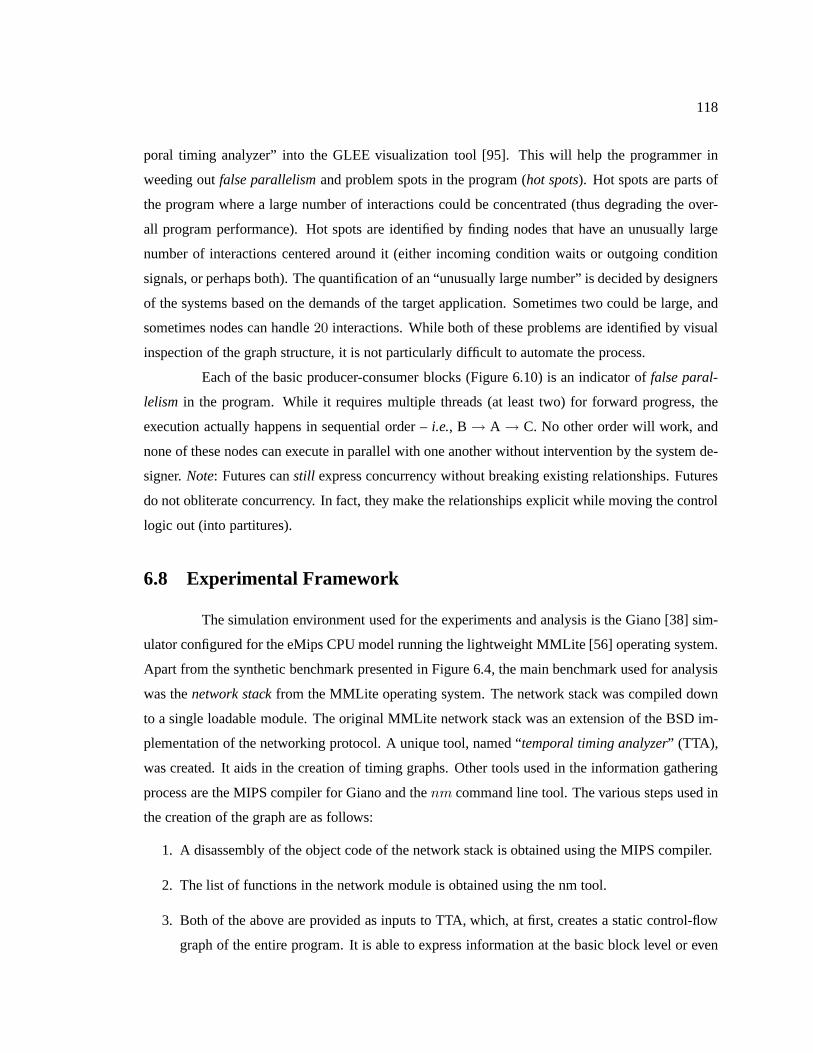
118

poral timing analyzer” into the GLEE visualization tool [95]. This will help the programmer in

weeding outfalse parallelismand problem spots in the program (hot spots). Hot spots are parts of

the program where a large number of interactions could be concentrated (thus degrading the over-

all program performance). Hot spots are identified by findingnodes that have an unusually large

number of interactions centered around it (either incomingcondition waits or outgoing condition

signals, or perhaps both). The quantification of an “unusually large number” is decided by designers

of the systems based on the demands of the target application. Sometimes two could be large, and

sometimes nodes can handle20 interactions. While both of these problems are identified byvisual

inspection of the graph structure, it is not particularly difficult to automate the process.

Each of the basic producer-consumer blocks (Figure 6.10) isan indicator offalse paral-

lelism in the program. While it requires multiple threads (at leasttwo) for forward progress, the

execution actually happens in sequential order –i.e., B→ A → C. No other order will work, and

none of these nodes can execute in parallel with one another without intervention by the system de-

signer.Note: Futures canstill express concurrency without breaking existing relationships. Futures

do not obliterate concurrency. In fact, they make the relationships explicit while moving the control

logic out (into partitures).

6.8 Experimental Framework

The simulation environment used for the experiments and analysis is the Giano [38] sim-

ulator configured for the eMips CPU model running the lightweight MMLite [56] operating system.

Apart from the synthetic benchmark presented in Figure 6.4,the main benchmark used for analysis

was thenetwork stackfrom the MMLite operating system. The network stack was compiled down

to a single loadable module. The original MMLite network stack was an extension of the BSD im-

plementation of the networking protocol. A unique tool, named “temporal timing analyzer” (TTA),

was created. It aids in the creation of timing graphs. Other tools used in the information gathering

process are the MIPS compiler for Giano and thenm command line tool. The various steps used in

the creation of the graph are as follows:

1. A disassembly of the object code of the network stack is obtained using the MIPS compiler.

2. The list of functions in the network module is obtained using the nm tool.

3. Both of the above are provided as inputs to TTA, which, at first, creates a static control-flow

graph of the entire program. It is able to express information at the basic block level or even

119

at a higher function level. The TTA is also able to determine the static dependencies among

the various basic blocks/functions in the program,i.e., it generates the green nodes and some

of the blue nodes of the timing graph. It is also able to provide an estimate of the yellow and

black edges in the graph.

4. A dynamic trace of the network stack running on Giano is obtained. The inputs are various

web service calls that trigger different functionality in the network. While this does not

guarantee complete dynamic coverage of the network stack, it is able to obtain a number of

dynamic dependencies (function pointers) and is also able to match many condition variables

to their wait/signal sites. These traces and the information gleaned from them are fed into the

TTA, which is able to form a more complete picture of the timing graph. From the dynamic

traces it is possible to restrict some yellow edges to blue edges while completely removing

some other yellow edges (as explained in Section 6.5). From information on the wait/signals

on condition variables, the TTA is also able to change some ofthe red edges to black edges

and eliminate other impossible black edges. In fact, if it ispossible to determine the entire

range of possible inputs for a function/application, then tracing will be able to provide a

complete picture of the dynamic behavior of the application.

5. Type analysis is performed and the information is then fedinto TTA. This adds more infor-

mation to the timing graph.

6. Information from other sources, such as domain knowledge, abstract executionetc. (Section

6.5) can also be plugged in to obtain a more comprehensive graph.

Any static timing analysis framework [86, 136] can be plugged in to the TTA to obtain

the WCETs for the green nodes after step(b). Step (e) was performed by hand and did not imple-

ment (f). The purpose of the experimental framework is to show that creation of the timing graph

using information collected from various sources is entirely feasible, which it did, as indicated in

the results section (Section 6.9). In fact, the design of TTAis such that it can be provided with in-

formation about the graph from any of the above mentioned (oreven other sources), which will then

be plugged into the graph to obtain a better understanding ofthe timing and runtime behavior of the

application. The most interesting part about the analysis (graph reductions and subsequent obser-

vations) is that it can be performed on an incomplete graph aswell as a graph which has all of its

characteristics mapped. While the former will yield approximate results, the latter can yield precise

results. These insights (on the state of the concurrency, sequentialization and resource constraints

120

of the application) can greatly assist programmers and system designers.

6.9 Results

Section 6.9.1 enumerates the results obtained by performing the transformations and anal-

yses on the timing graph. Section 6.9.2 lists results obtained from the temporal timing analyzer

showing that the process of creating the timing graph is a feasible one.

6.9.1 Graph Results

The following insights were obtained by performing the various analyses and transforma-

tions on the timing graph:

• The most important and perhaps most surprising result is that increasing the concurrencyof

the timing graph, using certain program modifications, resulted in increased serializability.

This provides the scheduler with a lot of flexibility in creating the final schedule and tailoring

it to the particular hardware system in use.

• Various graph transformations finally lead to three types ofgraphs – those that can be com-

pletely serialized, those that resulted in deadlocks and those that are constructed of basic

producer-consumer relationships. The last result shows that it is possible to calculate the min-

imum resource requirements (threads and corresponding execution stacks) for correct forward

progress in the program. This results in memory usage reduction in embedded systems.

• The analysis is able to direct the programmer’s attention towards false parallelism and hot

spots in the program.

• The final graph is the worst-case schedule possible for the program.

• The graph reduction shows that it is possible to minimize thenumber of context switches in

the application.

• Inter-thread communication/dependencies are reduced.

• The transformations result in the smallest partiture.

• The graph helps programmers visualize and understand the application. This will tell them if

their original design was correctly translated into code and perhaps even show them if there

were any deficiencies in the original design.

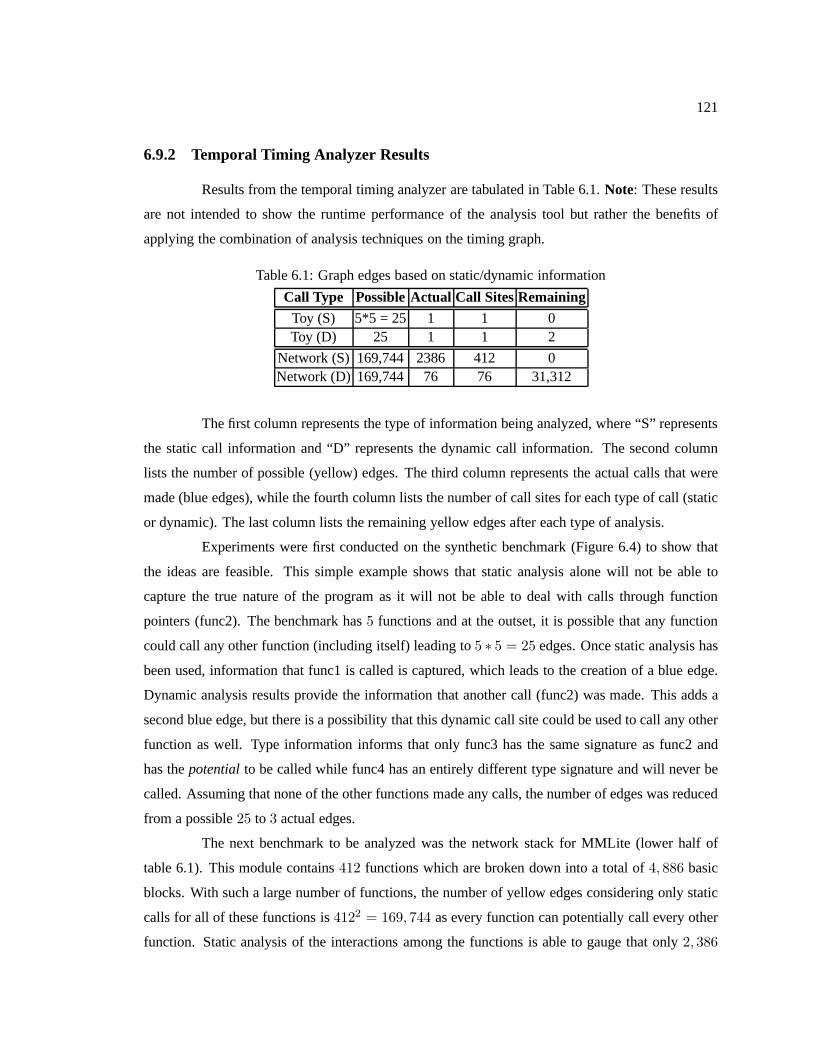
121

6.9.2 Temporal Timing Analyzer Results

Results from the temporal timing analyzer are tabulated in Table 6.1.Note: These results

are not intended to show the runtime performance of the analysis tool but rather the benefits of

applying the combination of analysis techniques on the timing graph.

Table 6.1: Graph edges based on static/dynamic information

Call Type PossibleActual Call SitesRemaining

Toy (S) 5*5 = 25 1 1 0Toy (D) 25 1 1 2

Network (S) 169,744 2386 412 0Network (D) 169,744 76 76 31,312

The first column represents the type of information being analyzed, where “S” represents

the static call information and “D” represents the dynamic call information. The second column

lists the number of possible (yellow) edges. The third column represents the actual calls that were

made (blue edges), while the fourth column lists the number of call sites for each type of call (static

or dynamic). The last column lists the remaining yellow edges after each type of analysis.

Experiments were first conducted on the synthetic benchmark(Figure 6.4) to show that

the ideas are feasible. This simple example shows that static analysis alone will not be able to

capture the true nature of the program as it will not be able todeal with calls through function

pointers (func2). The benchmark has5 functions and at the outset, it is possible that any function

could call any other function (including itself) leading to5 ∗ 5 = 25 edges. Once static analysis has

been used, information that func1 is called is captured, which leads to the creation of a blue edge.

Dynamic analysis results provide the information that another call (func2) was made. This adds a

second blue edge, but there is a possibility that this dynamic call site could be used to call any other

function as well. Type information informs that only func3 has the same signature as func2 and

has thepotentialto be called while func4 has an entirely different type signature and will never be

called. Assuming that none of the other functions made any calls, the number of edges was reduced

from a possible25 to 3 actual edges.

The next benchmark to be analyzed was the network stack for MMLite (lower half of

table 6.1). This module contains412 functions which are broken down into a total of4, 886 basic

blocks. With such a large number of functions, the number of yellow edges considering only static

calls for all of these functions is4122 = 169, 744 as every function can potentially call every other

function. Static analysis of the interactions among the functions is able to gauge that only2, 386

122

functions were called statically by all412 functions. This converts2, 386 of the yellow edges to

blue edges and also eliminates all of the remaining169, 744 − 2, 386 = 167, 358 ones.

Similar results are presented for dynamic calls. The remaining yellow edges were cal-

culated as follows: Each one of the76 call sites can potentially call any one of the412 functions

leading to76 ∗ 412 = 31, 312 possible yellow edges. Type analysis now calculates that only func-

tions that match the signature of these76 callees can ever be called from these dynamic call sites,

which leads to a further reduction in the number of possible edges. Domain knowledge can further

reduce this number as some of these “potential” callees (with function signature matches) cannot be

called during the same execution instance. Hence, the number of edges drop further.

Hence, the initial estimates of339, 488 potential edges (static + dynamic) have been re-

duced to a more manageable one that is in the tens of thousands, if not less – an order of a magnitude

(or more) difference. Hence, analysis of complex programs using the TTA framework and graph

transformation techniques is feasible. It is able to handlelarge programs, which, to date, have been

excluded from such analyses due to their inherent complexity. Note: These are not claims of re-

ducing thetime complexityof these programs. Such programs were considered to be inherently

un-analyzable due to the programmatic constructs they contain (e.g., function pointers). In the past,

analysis of such programs would not have been possible by anyone of static analysis, dynamic

analysis, type information, domain knowledge alone. In this work, it was achieved as a result of

combining all these methods.

6.10 Conclusion

This chapter presented a combination of analysis tools and methods to glean informa-

tion from programs and then combined them into a graph. The graph represents a model of the

temporal behavior of a program. This chapter defines the graph coloring, invariants, and a set of

valid transformations that are used to extract informationout of the graph. One insight gained was

that increasing the concurrency of the application can leadto increased serializability. The graph

could be output as a partiture that is usable as a manifesto ofthe program behavior as well as in

scalable and distributed scheduling. This chapter also extended the reach of static timing analysis

to applications that were, due to their complexity, not previously analyzable for determination of

worst-case behavior. This was done by combining static analysis with dynamic analysis based on

traces and with other techniques, such as type inference. The practicality of the graph generation

and analysis methods were demonstrated with an implementation that was used to create a graph of

123

an entire TCP/IP stack. The topological properties that thegraph transformations reveal are useful

in understanding and optimizing an application for variable levels of parallelism. The methodology

presented here forms a solid base for further work in schedulability analysis.

124

Chapter 7

Related Work

This dissertation aims to present analysis techniques for modern embedded systems along

three broad areas as presented in Chapters 2 – 6. This chapteron related work is also split along

these lines but first, Sections 7.1 – 7.4 present an overview of the field of timing analysis.

Section 7.5 presents research related to the CheckerMode concept that deals with attempts

to analyze contemporary architectures. Section 7.6 presents literature that deals with reducing con-

straints on the development of embedded software and the useof such techniques in reducing power

consumption. Section 7.7 presents other attempts to analyze distributed embedded and real-time

systems.

7.1 WCET Requirements

Knowledge of worst-case execution times (WCETs) is necessary for most hard real-time

systems. The WCET must be known or safely bounda priori so that the feasibility of schedul-

ing task sets in the system may be determined based on a scheduling policy (e.g., rate-monotone

or earliest-deadline-first scheduling [76]). The WCET values obtained by the process oftiming

analysisare required to be

1. Safe: They shouldneverunderestimate the actual WCET of the task. Failure to do so could

result in catastrophic failures to the system putting humanbeings, their environment, or both

in danger.

2. Tight : The overestimations in the WCET calculation should be minimized as much as pos-

sible. This is aimed at reducing a wastage of resources because the scheduling policy, in

125

general, must account for the worst-case execution time forevery task in the system, po-

tentially resulting in infeasible task sets whose deadlines cannot be guaranteed (even though

those task sets never exceed their deadlines in practice).

Methods to obtain upper bounds on execution time range fromstatic analysis (safe but

not always tight) todynamic(but unsafe [126]) observations. Recently,hybrid methods have been

proposed as a way to obtain accurate WCETs for complex architectures.

7.2 Static Timing Analysis

The process of static timing analysis can be broadly described as containing the following

steps or phases:

1. Program analysis: This phase break down the program into its constituent parts. These parts,

depending on the analysis, could be basic blocks, paths, functions,etc.The information could

be represented in a variety of ways, fore.g., control flow graphs (CFG), tables, mathematical

expressions,etc.

2. Low-level/architectural analysis: In this step, the timing for some or all of the above “parts”

is obtained on an architectural (pipeline/processor) model(s).

3. Calculation/combination: This final phase combines the low-level results in an orderly fash-

ion to obtain the WCET for larger constructs – functions, libraries, tasks,etc.This can be done

explicitly by matching execution times to actual paths and then propagating the results to cal-

culate WCETs for the larger constructs. A timing tree is constructed such that each loop (or

function) corresponds to a node in the tree. The tree is processed in a bottom-up manner (the

WCET for an inner loop is calculated before that of an outer loop nest). The root of the tree

corresponds to the WCET for the entire task or module. This phase could also be performed

in an “implicit” manner using Integer Linear Programming (ILP) techniques.

Past work mainly focuses onstatic timing analysis techniques [14, 15, 26, 27, 34, 36, 49,

52,53,59,73,74,82,84,89,94,97,103,119,126,133]. Methods of analysis range from unoptimized

programs on simple CISC processors over optimized programson pipelined RISC processors and

uncached architectures to instruction and data caches. Harmon et al. [49] use time consuming

reverse-engineering methods that require error-prone data acquisition methods with,e.g.an oscillo-

scope, to obtain WCET values.

126

The static timing analysis framework that originated from Florida State University [52,

53,70,84,89,94,132,133] relies on accurate knowledge of:(a) the pipeline model/behavior;(b) the

execution times for each individual instruction through the pipeline; and(c) exactstatic knowledge

of the order of instruction scheduling within the pipeline.While (b) can be obtained by studying the

processor manuals, (a) and (c) are harder to model/understand, especially in the face of processor

features that introduce non-determinism, such as out-of-order processing.

Bernat and Burns proposed algebraic [14] expressions to represent the WCET of pro-

grams. Bernatat el. [15] used probabilistic approaches to express execution bounds down to the

granularity of basic blocks that could be composed to form larger program segments. Yet, the

combiner functions are not without problems, and timing of basic blocks requires architectural

knowledge similar to static timing analysis tools.

Implicit path enumeration techniques (IPET) [72, 136] apply path constraints to an exe-

cution graph by expressing them as inequalities. They calculate the execution times and number of

times each statement (or “part”) of the program executes using CPU models and run-time informa-

tion. This information is then fed into integer linear program (ILP) solvers to find the worst-case

number of executions for each program part. IPET techniquesallow infeasible paths to be elimi-

nated, handling of loops (simple and complex) and recursion, but suffer from some serious draw-

backs. These techniques still require some CPU models and run-time information (execution times

and number of executions for most program “parts.”) There isalso a price to pay in time complexity

because the ILP solvers used to solve these constraints, in general, areNP-hard.

Li et al. [71] present an integer linear programming (ILP) techniqueto handle cache

misses, speculative execution and branch prediction in WCET analysis. They consider various com-

binations of cache hits/misses and branch predictions/mispredictions. Only one outstanding branch

and one outstanding cache miss is considered at a time. This may not be an accurate representation

of a modern microprocessor where more than one branch might be outstanding. The ILP formula-

tion occurs alongside the creation of a Cache-Conflict Graph(CCG). Also, excessive time will be

required to formulate and solve the ILP equations. Althoughthis paper works toward analyzing

some of the difficult-to-analyze features of modern microprocessors (viz. caches and speculative

branches), it does not cover microprocessors with dynamic scheduling and out-of-order execution,

which can actually be captured using CheckerMode.

127

7.3 Dynamic and Stochastic Timing Analysis

Dynamictiming analysis methods [14, 15, 19, 119, 125, 127] are basedon trace-driven,

experimental or stochastic methods. Also, evolutionary testing techniques [101, 125, 127, 128] are

being used to automatically calculate WCETs for embedded software. They all suffer from the same

drawback that theycannotguarantee the safety of the WCET values produced [126]. Architectural

complexities, difficulties in determining worst-case input sets and the exponential complexity of

performing exhaustive testing over all possible inputs arealso reasons why dynamic timing analysis

methods are infeasible in general.Note: These techniques may be used to obtain WCET values for

softreal-time systems where missing a deadline is not necessarily a catastrophic event.

Some early work has suggested probabilistic analysis [15,33,60,122] for handling WCET

variations due to software factors (such as data dependencyand history dependency). However,

these prior approaches for statistical WCET analysis did not model hardware execution time varia-

tions caused by process variations and cannot guarantee thesafety of the WCET values obtained.

7.4 Timing Anomalies

While Graham [44] was the first to introduce the concept oftiming anomalies, Lundqvist

et al. [80,81] presented their significance in WCET estimation:

“Consider the execution of a sequence of instructions containing two different caseswhere the latency of instructions is modified. In the first case, the latency is increasedby i clock cycles. In the second case, the latency is decreased byd clock cycles. LetC be the future change in execution time resulting from the increase or decrease of thelatency. Then,a timing anomaly is a situation where, in the first case,C > i or C < 0,or in the second case,C < d or C > 0.”

Hence, timing anomalies represent counter-intuitive effects on timing when trying to an-

alyze instruction flow through the processor. Lundqvistet al. introduced the following three types

of anomalies:

• Cache hits can be worse than cache misses in WCET analysis. This effect shows up in out-of-

order (OOO) instruction scheduling, which executes instructions (or groups of instructions)

in a greedy manner. Instructions missing (instead of hitting) in cache could force certain

groups of instructions to exhibit different ordering during execution thus resulting inreduced

execution times. A detailed example is presented by Lundqvist et al. ( [80] Figure 2).

128

• Cache miss penalties can be higher than expected. Static WCET analysis usually looks for

the longest sequence of execution through a program. This may not always be true as cache

misses on supposedly shorter paths could result in them being longer during execution, thus

invalidating the timing for the “longest” path ( [80] Figure3).

• Unbounded effects on the WCET may exist. Usually, changes inthe execution times of paths

can be bounded statically while computing WCETs for them. Lundqvistet al. showed that

dominoeffects could cause the effects to the WCET to be unbounded (e.g.the delay in WCET

is proportional to the number of iterations), thus making itdifficult to estimate the correct

WCET without danger of underestimation ( [80] Figure 4).

The concept of timing anomalies was extended and generalized by others [13, 34, 106,

109, 118, 130]. It was shown that timing anomalies are not necessarily restricted to OOO proces-

sors, cache replacement policies can affect the existence or effects of timing anomalies, unequal

overlapping resources can lead to timing anomalies,etc.The concept of timing anomalies was also

formalized and classified to fit into one of the following three types [106]:

• Scheduling Anomalies. Most timing anomalies fall into this category and often occur due to

thegreedynature of schedulers.

• Speculative Timing Anomalies: These occur at a higher, task level where task sets are influ-

enced by previous decisions of the scheduler.

• Cache Timing Anomalies: These are caused by unexpected cache behavior, such as the non-

local worst-case cache hit results in a different future cache state than the local worst-case

cache miss.

All of these effects make the process of timing analysis difficult. Any analysis technique

must be able to correctly handle timing anomalies that couldpotentially occur in the processor.

There are two broad methods to deal with timing anomalies while performing worst-case analysis:

1. Identify timing anomalies and points where they may occur. The effects of the anomalies

can then be accounted for in the worst-case schedule of instructions. This is extremely hard

to do because it would involve anexhaustivesearch ofall potential effectsof scheduling

each permutation of instructions. As the relevant literature shows, the effects of the anomaly

could occur at locations quite distant from the source of theanomaly, further complicating

the analysis.

129

2. Preservethe effect of the anomaly in the analysis. Ensure that the effects of the anomalies,

if any, are propagated through the analysis so they do not “disappear” when performing the

WCET estimation. This avoids the laborious process of trying to detect the anomalies and

their effects while ensuring that the WCETs obtained are safe and tight.

CheckerMode utilizes the latter method to correctly deal with timing anomalies. This is

illustrated in Chapter 3.

7.5 CheckerMode Related Work (Hybrid Techniques)

Recently, hybrid timing analysis methods [15,48,134] as well as hardware-related meth-

ods [8, 81] have been proposed. Yet, none of these approachescapture advanced hardware fea-

tures transparently while providing tight bounds. While static timing analysis methods or abstract

interpretation methods [117, 119] can provide reasonably tight bounds for branches that can be

statically analyzed, they are not able to provide tight bounds for execution along speculatively pre-

dicted branch directions at runtime or out-of-order instruction-issue pipelines. The complexity and

overhead of modeling the behavior of even moderately complex pipelines [54] and interactions of

instructions within them is high for any of these methods. Whitham [134] presents a combination of

hardware and software techniques to capture WCETs accurately for complex processors that avoids

problems with timing anomalies. Instruction scheduling iscarried out by the compiler and relies

on custom microcode executing in the processor. It might be difficult to convince processor ven-

dors to undergo such radical changes in their design becauseit leads to an expensive verification

process. They may also be unwilling to provide such internaldetails due to intellectual property

considerations. Also, as detailed in the introduction, each new processor design requires that the

model be manually adapted and cannot reflect fabrication-level timing variability within a processor

batch. CheckerMode, in contrast, automatically adapts with changing processor details, including

timing variations due to fabrication. CheckerMode fills this gap and contributes to high confidence

in embedded systems design for time-critical missions.

CheckerModeis closely related to two prior approaches. First, Bernatet al. [15] used

probabilistic approaches to express execution bounds downto the granularity of basic blocks, which

could then be composed to form larger program segments. Second, the VISA framework [8] sug-

gested architectural enhancements to gauge the progress ofexecution by sub-task partitioning and

exploiting intra-task slack with DVS techniques. CheckerMode combines the benefits of these two

130

prior approaches without their shortcomings. While performing analysis on paths, cycles are mea-

sured in a special execution mode of the processor that supports checkpoint/restart and unknown

value execution semantics to reflect proper architectural state and path coverage. While Bernat

struggled with considerable timing perturbation from instrumentation, CheckerMode is much less

intrusive. Instead of a VISA-likevirtual processoraround a complex core, CheckerMode is pro-

moted as a realistic feature building on existing internal processor buffers widely used for specula-

tion / precise event handling. Hence, this method is able to provide more precise results compared

to Bernat’s work. In contrast to VISA, CheckerMode is able tosupport hybrid timing analysis on

the actual processor core.

Lundqvist et al. [81] use symbolic execution with a tight integration of path analysis and

timing analysis to obtain accurate WCET estimates. They usethe concept of an“unknown” value to

account for register values and addresses that cannot be statically determined, just as CheckerMode

does. However, their work did not utilize a fixed point approach but rather required each iteration of

a loop to be symbolically executed. Furthermore, they did not propose any architectural modifica-

tions and focused on static timing analysis over the entire program within an architectural simulator

using in-order execution without dynamic branch prediction etc. The term “timing anomaly”,i.e.,

an anomaly in the execution of code in dynamically scheduledprocessors, stems from their work

(see discussion in Section 7.4).

CheckerMode contends that the instruction window may be large enough that even if in-

structions get blocked due to anomalies, other instructions, that are ready may execute, thus reducing

the overall execution time of the program. Thus, by taking a larger context (path) into account, one

can provably compensate for localized anomalies at a largerscale within CheckerMode.

Petters [99] measures the execution times of parts of the program on actual microproces-

sors to obtain an accurate WCET estimate. He uses measurement techniques using hardware/software

probes and interrupts to obtain the execution times. Software instrumentation and debug routines

are also employed for this purpose. The main drawback of these techniques is that they change

either the behavior or the timing of the programs being analyzed.E.g., instrumentation changes the

software behavior of the program and may require manual intervention, interrupts modify the timing

characteristics of the program, while hardware probes may not obtain accurate timing results. The

CheckerMode approach does not suffer from any of these drawbacks and will produce tight WCET

results.

Schneider [109] illustrates the combination of WCET analysis and schedulability (response-

time) analysis for applications and real-time operating systems. He also performs WCET analysis

131

for superscalar, out-of-order processors while mentioning “late-order” effects for pipelines. These

are basically the “timing anomalies” discussed earlier, yet he considers handling multiple tasks in

the system. The work being presented here does not consider multiple tasks in the system and con-

centrates on obtaining the WCETs for the complete executionof a single task. This WCET value

can be used to perform multiple-task scheduling as well. TheCheckerMode system can be extended

to include the capability to obtain WCETs for a multiple-task real-time system.

The CheckerMode approach combines the best features of static and dynamic analysis

required for obtaining WCET bounds for modern processors. Chapter 2 introduced thehybrid

timing analysis technique that obtains actual execution times for short paths on the actual hardware

and then combines these intermediate worst-case bounds, offline, using a static tool.

7.6 ParaScale Related Work

This section is focused on timing analysis work related to parametric timing analysis and

dynamic voltage scaling (DVS).

Chapmanet al. [26] used path expressions to combine a source-oriented parametric ap-

proach of WCET analysis with timing annotations, verifyingthe latter with the former. Bernat and

Burns proposed algebraic expressions to represent the WCETof programs [14]. Bernatat el. used

probabilistic approaches to express execution bounds downto the granularity of basic blocks that

could be composed to form larger program segments [15]. Yet,the combiner functions are not with-

out problems, and timing of basic blocks requires architectural knowledge similar to static timing

analysis tools.

Parametric timing analysis by Vivancoset al. [124] first introduced techniques to handle

variable loop bounds as an extension to static timing analysis. That work focuses on the use of static

analysis methods to derive parametric formulae to bound variable-length loops. The ParaScale work

presented here, in contrast, assesses the benefits of this work, particularly in the realm of power-

awareness.

The effects of DVS on WCET have been studied in the FAST framework [110] where,

parametrization was used to model the effect of memory latencies on pipeline stalls as processor

frequency is varied. Due to DVS and constant memory access times, a lower processor frequency

results in fewer cycles to access memory, which is reflected in WCET bounds in their FAST frame-

work. This work is orthogonal to the method of PTA. In the timing analyzer presented in Chapter 5,

these effects are not currently modeled. This does not affect the correctness of the approach since

132

WCET bounds are safe without such modeling, but they may not be tight, as shown in the FAST

framework. Hence, the benefits of parametric DVS may even be better than what is reported here.

The VISA framework suggested architectural enhancements to gauge progress of exe-

cution by sub-task partitioning and exploits intra-task slack with DVS techniques [7, 8]. Their

technique did not exploit parametric loops. ParaScale, in contrast, takes advantage of dynamically

discovered loop bounds and does not require any modifications at the micro-architecture level.

Lisper [75] used polyhedral flow analysis to specify the iteration space of loop nests and

express them as parametric integer programming problems tosubsequently derive a parametric

WCET formula suitable for timing analysis using IPET (Implicit Path Enumeration Technique).

Recent work by Byhlinet al. [24] underlines the importance of using parametric expressions to

support WCET analysis in the presence of different modes of execution. They parametrize their

WCET predictions for automotive software based on certain parameters, such as frame size. Their

work focuses on studying the relationship between parameters unique to modes of execution and

their effect on the WCET. Other work by Gheorghitaet al.[41] also promotes a parametric approach

but at the level of basic blocks to distinguish different worst-case paths. The ideas, in this chapter,

of using parametric expressions, predating any of this work, accurately bound the WCET values for

loops. This extends the applicability of static analysis to a new class of programs. These accurate

predictions at run-time are utilized for benefits such as power savings and admission of additional

tasks.

The most closely related work in terms of intra-task DVS is the idea of power management

points (PMPs) [1–3] where, path-dependent power management hints (PMHs) were used to aggre-

gate knowledge about “saved” execution time compared to theworst-case execution that would have

been imposed along different paths. This work differs in that it exploits knowledge aboutpastexe-

cution while ParaScale discovers loop bounds that then provides tighter bounds on past andfuture

execution within the same task. Their work is also evaluatedwith SimpleScalar, albeit with a more

simplistic power model (E = CV 2) while ParaScale assess power at the micro-architecture level us-

ing enhancements of Wattch [20] as well as a more accurate leakage model [64]. Again, ParaScale

results could potentially be improved by benefiting from knowledge about past execution, which

may lead to additional power savings. This is subject to future work.

An intra-tasks DVS algorithm that “discovers” the amount ofexecution left in the system

and appropriately modifies the frequency and voltage of the system is presented in [111]. Their work

depends on inserting various instrumentation points at compile time into various paths in the code.

Evaluation of these instrumentation points at runtime provides information about the paths taken

133

during execution and thepossibleamount of execution time left along that path similar to PMPs.

They insert instrumentation points inevery basic blockto determine the exact execution path, which

would incur a significant overhead during runtime. This may also affect the caching and, hence,

timing behavior of the task code. ParaScale differs significantly in that it only assess the amount of

execution time remainingonce(prior to entry into a parametric loop), thus incurring an overhead

only once. Hence, it is able to accurately gauge theamount of execution remaining with a single

overhead per loop and per task instance. It also estimates the new caching and timing behavior of

the code after the call to the intra-task scheduler by invoking the timing analysis framework on the

modified code until the parametric WCET formulae stabilize.Another technique presented in their

paper is that of ”L-type voltage scaling edges”. They utilize the idea that loops are often executed

for a smaller number of iterations than the worst-case scenario. During run-time, they discover the

actual number of loop iterations at loop exit and then gauge the number of cycles saved. In contrast,

parametric timing analysis determines loop savingsprior to loop entry and exploits savings early,

e.g., using DVS, such as in ParaScale. This difference is a significant advantage for the parametric

approach, particularly for tasks where a single loop nest accounts for most of the execution time.

7.7 Temporal Timing Analysis Related Work

The work presented in chapter 6 is unique in that it is able to transform large applications

into a graph representation on which transformations are applied to gather the “meaning” of the

program with the aim of making distributed embedded systemsmore scalable, primarily by creating

models of the program based on the ideas ofpartituresandfutures.

Helanderet al. [57] introduced the concepts of partitures and futures as building blocks

for model-based design of distributed embedded systems. While they focus on techniques to build

applications, using these techniques, from the ground up, the work in Chapter 6 aims to understand

and possibly transformexistingmulti-threaded embedded systems with temporal constraints into

that model. Along the way, it aims at providing useful information and hints to designers of such

systems to improve the quality and scalability of the application.

Andersson [9] studied the temporal behavior of embedded programs and also used dy-

namic traces to add more information to his analysis. This work differs from that presented in

Chapter 6 in that he creates a model of the application and uses model checking and regression

analysis coupled with dynamic traces to reason about the temporal characteristics of the program.

It stops with analyzing the impact of the behavior of the temporal characteristics of the program

134

and does not provide any further insights (like Section 6.7). The work in Chapter 6 also deals with

concurrent programs as part of the analysis.

The level of parallelism required by an application has beenexplored by Motuset al. [91,

92]. They focus on model-driven development where an engineer writes a timing model (Q model)

including educated guesses for minimum and maximum times ofprocesses in periodic applications

such as those found in telephone switches. The model is basedon processes and channels. While

the work in the previous chapter facilitates writing the model by hand, it may also be used to analyze

existing programs and does not require the processes to be periodic.

Henzingeret al.[58] introduced the idea of compiler-driven feasibility checking of schedul-

ing code. In their approach, the compiler creates an executable that represents the schedule, which

is then attached to the end of the task. This schedule is executed and validated each time the task is

invoked on specialized embedded hardware. The work from Chapter 6 creates partitures and futures

based on the analysis of timing graphs. Also, compared to them, this work is able to determine the

levels of parallelism and potential problem spots in the application, which could prove beneficial to

a large range of systems.

Previous work in timing analysis deals with either static ordynamic analysis. The Check-

erMode concept presented in Chapters 2 – 4 [86, 87] presenteda hybrid approach to performing

timing analysis. Chapter 6 is similar in that it is also a hybrid approach which uses information for

a variety of sources. The difference is that the latter is focused on finding the properties of inter-

actions among threads in concurrent programs (analysis of complex software) while CheckerMode

is focused on obtaining worst-case execution time results for modern, out-of-order processors. In

fact, the two techniques are complementary. The results from that framework (the WCETs) can be

plugged in to the temporal timing analyzer to obtain more precise results for applications running

on modern processors.

135

Chapter 8

Future Work

Since this dissertation was loosely split into three parts,ideas for future research are also

presented along those lines. Section 8.1 details potentialresearch ideas for tackling the complexities

of modern architectures. Sections 8.2 and 8.3 explain ideasfor improved analysis techniques to

handle complexities in embedded software. Section 8.4 discusses some interesting ideas that utilize

combinations of all the analyses presented here.

8.1 CheckerMode Future Work

Chapters 2 – 4 presented techniques to analyze and bound the worst-case behavior of

modern architectural features with a focus onout-of-order (OOO) pipelines. While the material

presented here tackled most major issues dealing with OOO pipelines, further analysis could help

reduce the pessimism and overheads of the analysis. Currently, snapshots are captured atevery

branch instruction as well as beforeeveryjoin point in the control flow graph (CFG). This greatly

increases the analysis complexity, especially if many branches occur very close to each other, or

in case of a large nesting depth for branches. A static analysis of the CFG could help in capturing

snapshots at acoarsergranularity by skipping some intermediate branches. The paths that then fall

between the snapshots must be examined along all alternating combinations of branches/joins. Per-

haps some annotations from the programmer could help guide the analysis towards certain branches

while avoiding others.

A simplifying assumption was made that allotherprocessor features are absent and that

the pipeline could be analyzed in isolation. The increased performance of OOO processors is due

to other processor features as much as it is due to the pipeline. Processor features, such asdynamic

136

branch prediction, instruction and data caches, prefetching, etc., go a long way in increasing the

performance of these processors. While the current analysis precludes these features, including

them in a future version will definitely help in making modernprocessors more acceptable for use

in embedded and real-time systems.

Thebranch predictoris definitely a feature that is worth examining. Unlike the pipeline,

though, the branch predictor isnot stateless. Every branch instruction that is encountered influ-

ences and is influenced by the predictor. Hence, any attempt at capturing snapshots for a dynamic

branch predictor like “G-share” [83] involves the dauntingtask of capturing and managing a large

amount of state. This is especially problematic if snapshots occur close to each other. Another issue

while dealing with branch predictors is related to “merging” snapshots. Since branch predictors are

typically bit patterns and/or counters, a strategy for merge cannot be as simplistic as the amaxfunc-

tion of two snapshots, which was what was used while dealing with pipelines. Another significant

research challenge has to do with the Not-A-Number (NaN) values for input-dependent branches.

How must the branch predictor be updated when the branch is input-dependent?

Caches(both instruction and data) are similar to the branch predictor in that they contain

a large amount of state that must be captured for a comprehensive snapshot policy. NaN values

present similar challenges: How must an access to the cache with a NaN address be treated? The

pessimistic approach is to assume thatall NaN accessesmissin cache and are sent to memory. This

could lead to serious overestimations since the number of NaN-based references will increase as the

program execution proceeds resulting in huge WCET overestimations, especially for larger, more

complex programs.

Perhaps both of the above (branch predictors and caches) canbe analyzed by capturing

incremental stateat each successive snapshot. The state of the entire component can perhaps be

captured at coarser intervals, thus speeding up the analysis significantly. But the issue of how to

deal with input-dependent values is still a significant hurdle in obtaining accurate WCET estimates

for processors with these features.

8.2 ParaScale Future Work

The work in Chapter 5 illustrated the use of parametric timing analysis in achieving power

savings. This work can be carried further to study the benefits of ParaScale with other dynamic

voltage algorithms. These techniques, along with the associated run-time information, could also

be used for admitting new (sporadic [77]) tasks into the system. Parametric analysis can also be

137

applied to calculate bounds on recursive functions.

8.3 Future Work for Analysis of Distributed Embedded Systems

Chapter 6 presented analysis techniques to understand the behavior of complex embedded

systems,i.e., those that are distributed in nature. The aim was to analyzeand eventually transform

existing multi-threaded applications to the partiture-future model so that the application can be

adapted to a given hardware configuration ranging from smallmicrocontrollers to modern multi-

core architectures. The focus in this work was to adapt applications tosmallersystems,i.e., those

with limitations on physical memory. This was achieved by decreasing the amount of parallelism

in the application. An interesting extension would be to do the opposite,i.e., study the effects

of adapting the application tolarger, more parallel systems (in particular multicore architectures).

This would requireincreasingthe parallelism of the application that would demand quite different

trade-offs as compared to the analysis presented here.

Two techniques aimed to improve the scalability of the application were mentioned in

Section 6.7.1,viz. to transform the application to get rid of interactions between threads or to change

all sequential dependencies to be concurrent dependenciesusing thefutureconstruct. An interesting

research challenge is toautomaticallydetermine which parts of the applications are targets for these

transformations, if any, and then to actually carry out the transformations. The latter will aid in the

process of automaticallyadaptingthe application to varying levels of hardware resources, such as

parallelism, memory,etc.

8.4 Combination of Hardware and Software Analysis Techniques

The various techniques presented in this dissertation can actually be combined to provide

for better analysis of modern embedded, real-time and cyber-physical systems. CheckerMode and

ParaScale could be utilized in the analysis for distributedembedded systems to obtain accurate

WCETs for code within single threads. Parametric analysis techniques could be used to calculate

the effects of function pointers and synchronization constructs,i.e., to provide formulae to describe

the bounds on the number ofpotential callees.ParaScale techniques could also be used to estimate

the power consumption for the target platforms. It could be used in combination with dynamic

voltage scaling (DVS) techniques for smaller distributed embedded systems. For more complex and

more powerful systems, ParaScale could be used with more comprehensive DVS schemes, such as

138

Lookahead [100], Greedy DVS [88],etc.

CheckerMode techniques could be enhanced to analyze multi-core architectures so that

correct WCET information is available when trying to adapt the application to the high-end domain.

Hence, a large amount of potential exists when trying to combine the analysis techniques presented

in this dissertation.

139

Chapter 9

Conclusion

The original aim of this dissertation (Section 1.8) was to show that while modern embed-

ded systems prove to be too complex for any single analysis technique, they can be dissected, and

their worst-case behavior can be captured using a combination of the very same techniques. The

work presented in Chapters 2 – 6, has shown this hypothesis tobe true, both on the hardware as

well as the software fronts. The following sections discussthis in more detail before delving into

the correctness of the dissertation hypothesis in Section 9.4.

9.1 Analysis Techniques for Modern Processors

The CheckerModeinfrastructure presented in Chapters 2 – 4 was developed to analyze

contemporary processors with the aim of calculating worst-case execution times (WCETs) for code

executing on them. It provides the foundation to make contemporary processors predictable and

analyzable so that they may be safely used in embedded and real-time systems.

Chapter 2 presents a high-level overview of, the motivationfor, and the design choices

behind CheckerMode. The main idea is that interactions between hardware and software (ahybrid

timing analysis technique) can be utilized to obtain safe and tight WCET values for embedded sys-

tems with modern processors. Sequences of code are extracted on the software side and dispatched

to execute on the actual processor. Minor enhancements to the microarchitecture of modern proces-

sors is suggested to aid in the process of capturing information (“state”) during the execution of the

given program fragments.

Capturing and restoring state (known as “snapshots”) in CheckerMode is a non-trivial

task, especially in the presence of timing anomalies. CheckerMode is able to correctly deal with

140

timing anomalies in that they are preserved during the analysis. This is particularly important as the

task of detecting a timing anomaly is quite difficult, and completely ignoring anomalies could lead

to incorrect WCET estimates, even leading to underestimations. A correct handling of structural

dependencies and data dependencies is also presented with the aim of preserving the worst-case

behavior of the program.

Analysis of loops, especially those with input-dependent bounds, is problematic mainly

due to the halting problem,i.e., how many iterations must be timed to obtained the WCET for

the loop? This was solved by use of a fixed point technique thatonly needs to analyze the loop

for a few iterations and is then able to extrapolate for the remaining iterations. This is achieved

via a combination of traditional fixed point timing analysistechniques and the snapshot scheme

from CheckerMode. This analysis shows that the process of trying to capture the behavior of loops

through an OOO pipeline demands that a significant amount of architectural state (retire stage and

the issue/execute stages) be captured. Hence, any attempt to perform such an analysis cannot be

oblivious or transparent to all internal details of the processor microarchitecture. Finally, the WCET

for the loop and the benchmark as a whole can be presented as a formula if the upper bounds on the

number of loop iterations is unknown.

Hence, CheckerMode has the ability to provide worst-case guarantees forout-of-order

pipelinesusing a combination of analysis techniques by utilizing interactions and passing of infor-

mation between the hardware and software. This moves forward the state-of-the-art in the design of

embedded systems as OOO processors can now be made availableto designers of such applications.

9.2 Reducing Constraints on Embedded Software

The requirement that loop bounds must be statically determined is relaxed in this part

of the dissertation, presented in Chapter 5. Parametric formulae are integrated into the process of

timing analysis. This is carried out without sacrificing safety or tightness of WCET bounds. The

parametric formulae are calculated using a fixed point approach and embedded into the task code

prior to entry into the parametric loop. The formulae areevaluated at run-timewhen actual loop

bounds are available. This information is then exploited toreduce the voltage and frequency of the

processor with the aim of achievingenergy savings. The process involves the use oftwoschedulers,

one inter-task and oneintra-taskscheduler. The latter evaluates the parametric formulae atrun-time

and then invokes the dynamic voltage scaling (DVS) technique to save power. The framework is

referred to asParaScale. Also presented is a new DVS algorithm named “Greedy DVS”.

141

The benefit of ParaScale is that it is able toreduce voltage and frequency levels as

execution proceeds. This is in sharp contrast to existing DVS techniques, whichincrease volt-

age/frequency values as deadlines approach, thus resulting in losing some of the gains achieved

through DVS. Power savings as high as66% – 80% are observed while using ParaScale in com-

bination with Greedy DVS compared to DVS-oblivious techniques. These savings closely match

those obtained by dynamic, aggressive DVS algorithms whilestill maintaining a low time complex-

ity and are easy to implement (as simple extensions of staticDVS algorithms). These savings are in

sharp contrast to those that can be achieved via conventional timing analysis since ParaScale is able

to utilize knowledge about thefutureexecution of the task.

Hence, parametric timing analysis expands the class of applications that can be analyzed

and, hence, used on a real-time system. Programmers are now free to create more complex ap-

plications. ParaScale utilizes run-time information coupled with static analysis formulae to better

characterize the worst-case behavior of modern embedded systems. This is in keeping with the

theme that such systems, which could not be analyzed before,are now amenable to analysis due to

the combination of techniques, both static and dynamic.

9.3 Analysis of Distributed Embedded Systems

Some embedded systems and many cyber-physical systems are oftendistributedin nature,

i.e., they have multiple threads of execution with synchronization/communication constructs pass-

ing information or forcing dependencies between them. Suchsystems are typically out of the reach

of either static or dynamic analysis techniques, but not beyond a combination of the two. Chapter 6

illustrates the use of a combination of analysis techniques(static analysis, dynamic/run-time anal-

ysis, type information, domain knowledge,etc.) to accurately characterize the true nature of such

applications.

Information from all of these analysis techniques feed intoa “timing graph” on which

transformations and reductions are carried out with the aimof trying to understand the underlying

behavior and suggest changes/improvements to the application. The goal was to adapt a complex,

distributed embedded system to a resource-constrained platform (especially constraints on physical

memory).

One significant result obtained from the analysis was thatincreasing the concurrency of

an application also increased its sequentiality.This will help in tailoring the application based on

the hardware demands by increasing the sequentiality for resource-constrained systems while the

142

concurrency is increased for more powerful systems (such asmulticore architectures).

This piece of work extends the reach of traditional static timing analysis. By use of a

combination of analysis techniques and sources of information. It becomes possible to study classes

of application that were previously considered to be “un-analyzable”, such as the network stack used

for the experiments in this work.

9.4 Correctness of the Dissertation Hypothesis

The aim of this dissertation (Section 1.8) was to show that hardware and software con-

structs that are complex and “un-analyzable” by any single analysis technique or information source,

can now be studied and understood using a combination of techniques. This dissertation has pro-

vided the means to analyze each of the constructs mentioned in the hypothesis:

1. Out-of-order processor pipelineshave shown to be analyzable using interactions between

hardware and software through theCheckerModeframework [86, 87]. This framework has

the ability to correctly preserve timing anomalies as well as handle loops without explicitly

enumerating all loop iterations. These techniques can be extended to analyze other parts of

the process (branch predictor, caches,etc.) in the future.

2. Embedded code withstatically indeterminate loop boundscan now be analyzed by using

static parametric timing analysis techniques coupled withrun-time information about the ac-

tual loop bounds through theParaScaleframework [88, 89]. The savings (slack) from this

technique were used to obtain a reduction in the energy consumption of the embedded sys-

tem.

3. Distributed embedded systemscan be analyzed by using information from static analysis,

run-time/dynamic traces, type analysis and domain knowledge through theTemporal Tim-

ing Analyzer (TTA)[85]. Graph-based analysis techniques can help in adaptingdistributed

embedded systems to a variety of hardware profiles.

Hence, the claims in the dissertation hypothesis have been shown to be correct.

143

Bibliography

[1] N. AbouGhazaleh, B. Childers, D. Mosse, R. Melhem, and Matthew Craven. Energy man-

agement for real-time embedded applications with compilersupport. InACM SIGPLAN

Conference on Language, Compiler, and Tool Support for Embedded Systems, June 2003.

[2] N. AbouGhazaleh, D. Mosse, B. Childers, and R. Melhem. Toward the placement of power

management points in real time applications. InWorkshop on Compilers and Operating

Systems for Low Power, September 2001.

[3] N. AbouGhazaleh, D. Mosse, B. Childers, R. Melhem, and Matthew Craven. Collaborative

operating system and compiler power management for real-time applications. InIEEE Real-

Time Embedded Technology and Applications Symposium, May 2003.

[4] Gagan Agrawal, Anurag Acharya, and Joel Saltz. An interprocedural framework for place-

ment of asynchronous I/O operations. InProceedings of the 10th ACM International Confer-

ence on Supercomputing, pages 358–365, Philadelphia, PA, 1996. ACM Press.

[5] A. V. Aho, R. Sethi, and J. D. Ullman.Compilers – Principles, Techniques, and Tools.

Addison-Wesley, 1986.

[6] N. Al-Yaqoubi. Reducing timing analysis complexity by partitioning control flow. Master’s

thesis, Florida State University, 1997. Master’s Project.

[7] A. Anantaraman, K. Seth, K. Patil, E. Rotenberg, and F. Mueller. Virtual simple architecture

(VISA): Exceeding the complexity limit in safe real-time systems. InInternational Sympo-

sium on Computer Architecture, pages 250–261, June 2003.

[8] A. Anantaraman, K. Seth, K. Patil, E. Rotenberg, and F. Mueller. Enforcing safety of real-

time schedules on contemporary processors using a virtual simple architecture (visa). In

IEEE Real-Time Systems Symposium, pages 114–125, December 2004.

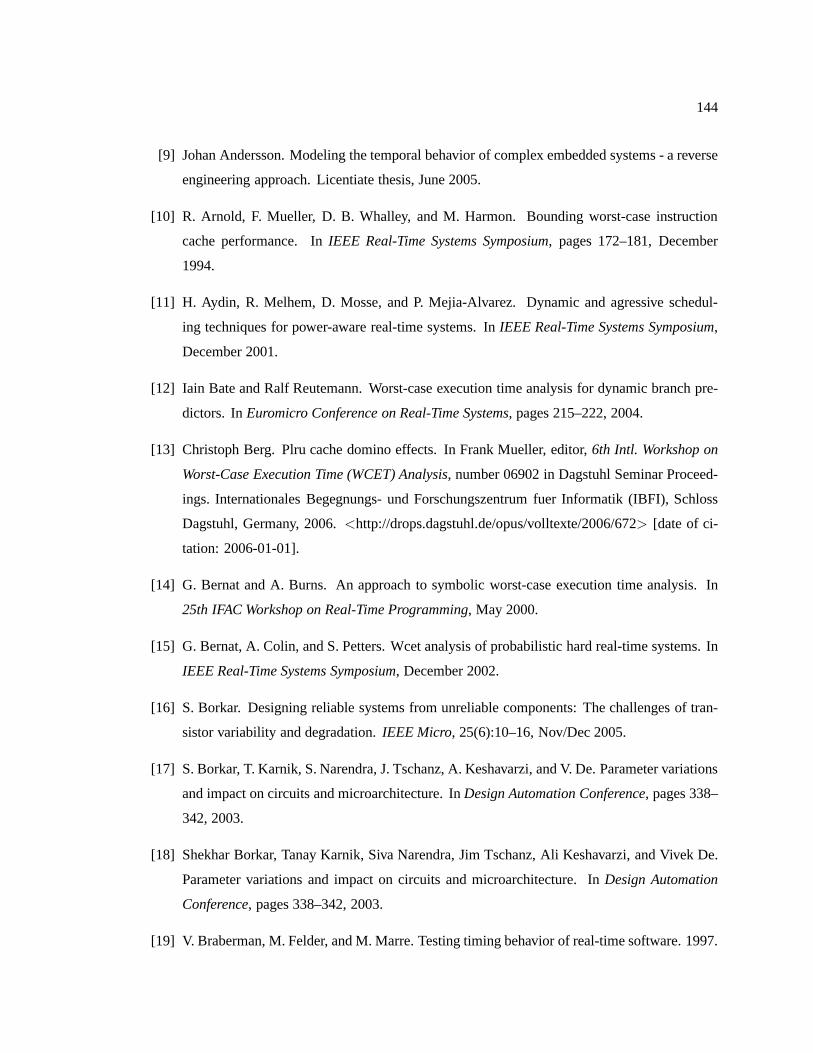
144

[9] Johan Andersson. Modeling the temporal behavior of complex embedded systems - a reverse

engineering approach. Licentiate thesis, June 2005.

[10] R. Arnold, F. Mueller, D. B. Whalley, and M. Harmon. Bounding worst-case instruction

cache performance. InIEEE Real-Time Systems Symposium, pages 172–181, December

1994.

[11] H. Aydin, R. Melhem, D. Mosse, and P. Mejia-Alvarez. Dynamic and agressive schedul-

ing techniques for power-aware real-time systems. InIEEE Real-Time Systems Symposium,

December 2001.

[12] Iain Bate and Ralf Reutemann. Worst-case execution time analysis for dynamic branch pre-

dictors. InEuromicro Conference on Real-Time Systems, pages 215–222, 2004.

[13] Christoph Berg. Plru cache domino effects. In Frank Mueller, editor,6th Intl. Workshop on

Worst-Case Execution Time (WCET) Analysis, number 06902 in Dagstuhl Seminar Proceed-

ings. Internationales Begegnungs- und Forschungszentrumfuer Informatik (IBFI), Schloss

Dagstuhl, Germany, 2006.<http://drops.dagstuhl.de/opus/volltexte/2006/672> [date of ci-

tation: 2006-01-01].

[14] G. Bernat and A. Burns. An approach to symbolic worst-case execution time analysis. In

25th IFAC Workshop on Real-Time Programming, May 2000.

[15] G. Bernat, A. Colin, and S. Petters. Wcet analysis of probabilistic hard real-time systems. In

IEEE Real-Time Systems Symposium, December 2002.

[16] S. Borkar. Designing reliable systems from unreliablecomponents: The challenges of tran-

sistor variability and degradation.IEEE Micro, 25(6):10–16, Nov/Dec 2005.

[17] S. Borkar, T. Karnik, S. Narendra, J. Tschanz, A. Keshavarzi, and V. De. Parameter variations

and impact on circuits and microarchitecture. InDesign Automation Conference, pages 338–

342, 2003.

[18] Shekhar Borkar, Tanay Karnik, Siva Narendra, Jim Tschanz, Ali Keshavarzi, and Vivek De.

Parameter variations and impact on circuits and microarchitecture. InDesign Automation

Conference, pages 338–342, 2003.

[19] V. Braberman, M. Felder, and M. Marre. Testing timing behavior of real-time software. 1997.

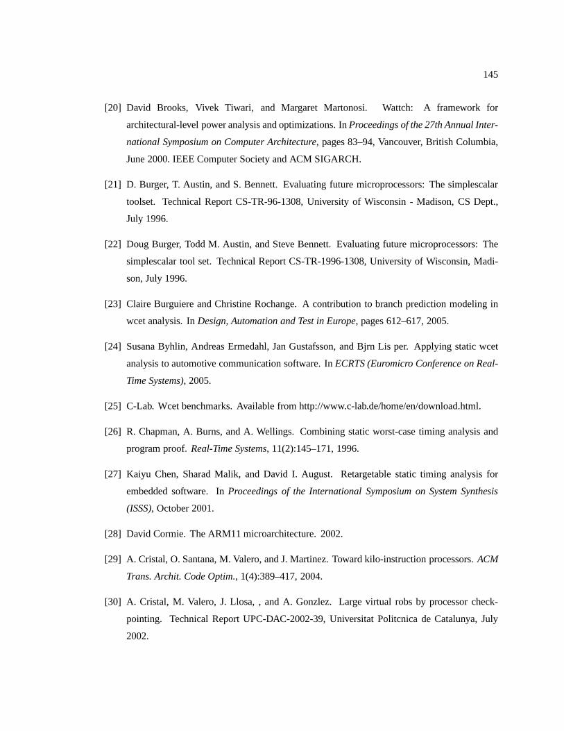
145

[20] David Brooks, Vivek Tiwari, and Margaret Martonosi. Wattch: A framework for

architectural-level power analysis and optimizations. InProceedings of the 27th Annual Inter-

national Symposium on Computer Architecture, pages 83–94, Vancouver, British Columbia,

June 2000. IEEE Computer Society and ACM SIGARCH.

[21] D. Burger, T. Austin, and S. Bennett. Evaluating futuremicroprocessors: The simplescalar

toolset. Technical Report CS-TR-96-1308, University of Wisconsin - Madison, CS Dept.,

July 1996.

[22] Doug Burger, Todd M. Austin, and Steve Bennett. Evaluating future microprocessors: The

simplescalar tool set. Technical Report CS-TR-1996-1308,University of Wisconsin, Madi-

son, July 1996.

[23] Claire Burguiere and Christine Rochange. A contribution to branch prediction modeling in

wcet analysis. InDesign, Automation and Test in Europe, pages 612–617, 2005.

[24] Susana Byhlin, Andreas Ermedahl, Jan Gustafsson, and Bjrn Lis per. Applying static wcet

analysis to automotive communication software. InECRTS (Euromicro Conference on Real-

Time Systems), 2005.

[25] C-Lab. Wcet benchmarks. Available from http://www.c-lab.de/home/en/download.html.

[26] R. Chapman, A. Burns, and A. Wellings. Combining staticworst-case timing analysis and

program proof.Real-Time Systems, 11(2):145–171, 1996.

[27] Kaiyu Chen, Sharad Malik, and David I. August. Retargetable static timing analysis for

embedded software. InProceedings of the International Symposium on System Synthesis

(ISSS), October 2001.

[28] David Cormie. The ARM11 microarchitecture. 2002.

[29] A. Cristal, O. Santana, M. Valero, and J. Martinez. Toward kilo-instruction processors.ACM

Trans. Archit. Code Optim., 1(4):389–417, 2004.

[30] A. Cristal, M. Valero, J. Llosa, , and A. Gonzlez. Large virtual robs by processor check-

pointing. Technical Report UPC-DAC-2002-39, UniversitatPolitcnica de Catalunya, July

2002.

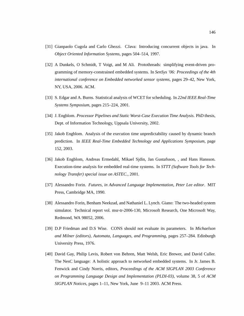
146

[31] Gianpaolo Cugola and Carlo Ghezzi. CJava: Introducingconcurrent objects in java. In

Object Oriented Information Systems, pages 504–514, 1997.

[32] A Dunkels, O Schmidt, T Voigt, and M Ali. Protothreads: simplifying event-driven pro-

gramming of memory-constrained embedded systems. InSenSys ’06: Proceedings of the 4th

international conference on Embedded networked sensor systems, pages 29–42, New York,

NY, USA, 2006. ACM.

[33] S. Edgar and A. Burns. Statistical analysis of WCET for scheduling. In22nd IEEE Real-Time

Systems Symposium, pages 215–224, 2001.

[34] J. Engblom.Processor Pipelines and Static Worst-Case Execution Time Analysis. PhD thesis,

Dept. of Information Technology, Uppsala University, 2002.

[35] Jakob Engblom. Analysis of the execution time unpredictability caused by dynamic branch

prediction. InIEEE Real-Time Embedded Technology and Applications Symposium, page

152, 2003.

[36] Jakob Engblom, Andreas Ermedahl, Mikael Sjdin, Jan Gustafsson, , and Hans Hansson.

Execution-time analysis for embedded real-time systems. In STTT (Software Tools for Tech-

nology Transfer) special issue on ASTEC., 2001.

[37] Alessandro Forin.Futures, in Advanced Language Implementation, Peter Lee editor. MIT

Press, Cambridge MA, 1990.

[38] Alessandro Forin, Benham Neekzad, and Nathaniel L. Lynch. Giano: The two-headed system

simulator. Technical report vol. msr-tr-2006-130, Microsoft Research, One Microsoft Way,

Redmond, WA 98052, 2006.

[39] D.P Friedman and D.S Wise. CONS should not evaluate its parameters. InMichaelson

and Milner (editors), Automata, Languages, and Programming, pages 257–284. Edinburgh

University Press, 1976.

[40] David Gay, Philip Levis, Robert von Behren, Matt Welsh,Eric Brewer, and David Culler.

The NesC language: A holistic approach to networked embedded systems. In Jr. James B.

Fenwick and Cindy Norris, editors,Proceedings of the ACM SIGPLAN 2003 Conference

on Programming Language Design and Implementation (PLDI-03), volume 38, 5 ofACM

SIGPLAN Notices, pages 1–11, New York, June 9–11 2003. ACM Press.

147

[41] Valentin S. Gheorghita, Sander Stuijk, Twan Basten, and Henk Corporaal. Automatic sce-

nario detection for improved wcet estimation. InDesign Automation Conference, June 2005.

[42] John B. Goodenough and Lui Sha. The priority ceiling protocol: A method for minimizing

the blocking of high priority Ada tasks. InProceedings of the 2nd International Workshop

on Real-Time Ada Issues, May 1988.

[43] K. Govil, E. Chan, and H. Wasserman. Comparing algorithms for dynamic speed-setting of

a low-power cpu. In1st Int’l Conference on Mobile Computing and Networking, Nov 1995.

[44] Ronald L. Graham. Bounds on multiprocessing timing anomalies. InIAM Journal of Applied

Mathematics, 1969.

[45] F. Gruian. Hard real-time scheduling for low energy using stochastic data and dvs proces-

sors. InProceedings of the International Symposium on Low-Power Electronics and Design

ISLPED’01, Aug 2001.

[46] D. Grunwald, P. Levis, C. Morrey III, M. Neufeld, and K. Farkas. Policies for dynamic clock

scheduling. InSymp. on Operating Systems Design and Implementation, Oct 2000.

[47] Robert Halstead. MULTILISP: a language for concurrentsymbolic computation.ACM Trans.

Program. Lang. Syst., 7(4):501–538, 1985.

[48] A. Hamann, M. Jersak, K. Richter, and R. Ernst. Design space exploration and system op-

timization with symta/s - symbolic timing analysis for systems. InIEEE Real-Time Systems

Symposium, pages 469–478, December 2004.

[49] M. Harmon, T. P. Baker, and D. B. Whalley. A retargetabletechnique for predicting execution

time. In IEEE Real-Time Systems Symposium, pages 68–77, December 1992.

[50] C. Healy, M. Sjodin, V. Rustagi, D. Whalley, and R. van Engelen. Supporting timing analysis

by automatic bounding of loop iterations.Real-Time Systems, 18(2/3):121–148, May 2000.

[51] C. A. Healy, R. D. Arnold, F. Mueller, D. Whalley, and M. G. Harmon. Bounding pipeline

and instruction cache performance.IEEE Transactions on Computers, 48(1):53–70, January

1999.

148

[52] C. A. Healy, M . Sjodin, and D. B. Whalley. Bounding loopiterations for timing analysis.

In IEEE Real-Time Embedded Technology and Applications Symposium, pages 12–21, June

1998.

[53] C. A. Healy, D. B. Whalley, and M. G. Harmon. Integratingthe timing analysis of pipelining

and instruction caching. InIEEE Real-Time Systems Symposium, pages 288–297, December

1995.

[54] Reinhold Heckmann, Marc Langenback, Stephan Thesing,and Reinhard Wilhelm. The in-

fluence of processor architecture on the design and the results of WCET tools.Proceedings

of the IEEE, pages 1038–1054, July 2003.

[55] Johannes Helander. Deeply embedded XML communication: Towards an interoperable and

seamless world. In5th ACM Conference on Embedded Software‘, September 2005.

[56] Johannes Helander and Alessandro Forin. MMLite: A highly componentized system archi-

tecture. InProceedings of the ACM SIGOPS European Workshop on Support for Composing

Distributed Applications, 1998.

[57] Johannes Helander, Risto Serg, Margus Veanes, and Pritam Roy. Adapting futures: Scalabil-

ity for real-world computing. InReal-Time Systems Symposium, December 2007.

[58] Tom Henzinger, Christoph Kirsch, and Slobodan Matic. Schedule carrying code. InThird

International Conference on Embedded Software (EMSOFT), January 2003.

[59] Andre Hergenhan and Wolfgang Rosenstiel. Static timing analysis of embedded software on

advanced processor architectures. InDATE, pages 552–559, 2000.

[60] X. S. Hu, Z. Tao, and E. H. M. Sha. Estimating probabilistic timing performance for real-

time embedded systems.Very Large Scale Integration (VLSI) Systems, IEEE Transactions

on, 9(6):833–844, 2001. 1063-8210.

[61] P. Hurat, Y.-T. Wang, and N.K. Vergese. Sub-90 nanometer variability is here to stay.EDA

Tech Forum, 2(3):26–28, September 2005.

[62] Jonathan Jacky, Margus Veanes, Colin Campbell, and Wolfram Schulte. Model-based soft-

ware testing and analysis with c#. InCmbridge Univeristy Press, 2007.

149

[63] R. Jejurikar and R. Gupta. Dynamic slack reclemation with procrastination scheduling in

real-time embedded systems. InDesign Automation Conference, June 2005.

[64] R. Jejurikar, C. Pereira, and R. Gupta. Leakage aware dynamic voltage scaling for real-time

embedded systems. InDesign Automation Conference, June 2004.

[65] D. Kang, S. Crago, and J. Suh. A fast resource synthesis technique for energy-efficient real-

time systems. InIEEE Real-Time Systems Symposium, December 2002.

[66] Alvin R. Lebeck, Jinson Koppanalil, Tong Li, Jaidev Patwardhan, and Eric Rotenberg. A

large, fast instruction window for tolerating cache misses. In ISCA ’02: Proceedings of the

29th annual international symposium on Computer architecture, pages 59–70, Washington,

DC, USA, 2002. IEEE Computer Society.

[67] C. Lee, J. Hahn, Y. Seo, S. Min, R. Ha, S. Hong, C. Park, M. Lee, and C. Kim. Analysis of

cache-related preemption delay in fixed-priority preemptive scheduling. InIEEE Real-Time

Systems Symposium, December 1996.

[68] Cheol-Hoon Lee and Kang G. Shin. On-line dynamic voltage scaling for hard real-time

systems using the edf algorithm. InIEEE Real-Time Embedded Technology and Applications

Symposium, June 2004.

[69] Yann-Hang Lee and C. M. Krishna. Voltage-clock scalingfor low energy consumption in

fixed-priority real-time systems.Real-Time Syst., 24(3):303–317, 2003.

[70] Joseph Y-T. Leung. A new algorithm for scheduling periodic, real-time tasks. to appear in

Journal of Algorithmica.

[71] Xianfeng Li, Tulika Mitra, and Abhik Roychoudhary. Accurate timing analysis by modeling

caches, speculation and their interaction. InProceedings of the Design Automation Confer-

ence, 2003.

[72] Y.-T. S. Li, S. Malik, and A. Wolfe. Efficient microarchitecture modeling and path analysis

for real-time software. InIEEE Real-Time Systems Symposium, pages 298–397, December

1995.

[73] Y.-T. S. Li, S. Malik, and A. Wolfe. Cache modeling for real-time software: Beyond di-

rect mapped instruction caches. InIEEE Real-Time Systems Symposium, pages 254–263,

December 1996.

150

[74] S.-S. Lim, Y. H. Bae, G. T. Jang, B.-D. Rhee, S. L. Min, C. Y. Park, H. Shin, and C. S. Kim.

An accurate worst case timing analysis for RISC processors.In IEEE Real-Time Systems

Symposium, pages 97–108, December 1994.

[75] Bjorn Lisper. Fully automatic, parametric worst-case execution time analysis. InWCET,

pages 99–102, 2003.

[76] C. Liu and J. Layland. Scheduling algorithms for multiprogramming in a hard-real-time

environment.J. of the Association for Computing Machinery, 20(1):46–61, January 1973.

[77] J. Liu. Real-Time Systems. Prentice Hall, 2000.

[78] Yanbin Liu and Aloysius K. Mok. An integrated approach for applying dynamic voltage

scaling to hard real-time systems. InProceedings of the ninth IEEE Real-Time and Embedded

Technology and Applications Symposium, May 2003.

[79] T. Lundqvist and P. Stenstrom. An integrated path and timing analysis method based on

cycle-level symbolic execution.Real-Time Systems, 17(2/3):183–208, November 1999.

[80] Thomas Lundqvist and Per Stenstrom. Timing anomaliesin dynamically scheduled micro-

processors. InRTSS ’99: Proceedings of the 20th IEEE Real-Time Systems Symposium,

page 12, Washington, DC, USA, 1999. IEEE Computer Society.

[81] Thomas Lunqvist. A WCET Analysis Method for Pipelined Microprocessors with Cache

Memories. PhD thesis, Chalmers University, 2002.

[82] Sharad Malik, Margaret Martonosi, and Yau-Tsun StevenLi. Static timing analysis of em-

bedded software. InProceedings of the 34th Conference on Design Automation (DAC-97),

pages 147–152, NY, June 1997. ACM Press.

[83] Scott McFarling. Combining Branch Predictors. Technical Report TN-36, June 1993.

[84] S. Mohan, F. Mueller, D. Whalley, and C. Healy. Timing analysis for sensor network nodes

of the atmega processor family. InIEEE Real-Time Embedded Technology and Applications

Symposium, pages 405–414, March 2005.

[85] Sibin Mohan and Johannes Helander. Temporal analysis for adapting concurrent applications

to embedded systems. InEuromicro Conference on Real-Time Systems, July 2008.

151

[86] Sibin Mohan and Frank Mueller. Hybrid timing analysis of modern processor pipelines via

hardware/software interactions. InIEEE Real-Time Embedded Technology and Applications

Symposium, April 2008.

[87] Sibin Mohan and Frank Mueller. Merging state and preserving timing anomalies in pipelines

of high-end processor. InIEEE Real-Time Systems Symposium, (submitted to) 2008.

[88] Sibin Mohan, Frank Mueller, Will Hawkins, Michael Root, David Whalley, and Chris Healy.

Parametric timing analysis and its application to dynamic voltage scaling.ACM Transactions

on Embedded Computing Systems (TECS), accepted in 2007.

[89] Sibin Mohan, Frank Mueller, William Hawkins, Michael Root, Christopher Healy, and David

Whalley. Parascale: Expoliting parametric timing analysis for real-time schedulers and dy-

namic voltage scaling. InIEEE Real-Time Systems Symposium, pages 233–242, December

2005.

[90] D. Mosse, H. Aydin, B. Childers, and R. Melhem. Compiler-assisted dynamic power-aware

scheduling for real-time applications. InWorkshop on Compilers and Operating Systems for

Low Power, October 2000.

[91] L. Motus, R. Kinksaar, T. Naks, and M. Pall. Enhancing object modelling technique with

timing analysis capabilities.iceccs, 00:298, 1995.

[92] Leo Motus and Michael G. Rodd.Timing Analysis of Real-Time Software: A Practical Ap-

proach to the Specification and Design of Real-Time. Elsevier Science Inc., New York, NY,

USA, 1994.

[93] T. Mowry and C.-K. Luk. Predicting data cache misses in non-numeric applications through

correlation profiling. InMICRO-30, pages 314–320, December 1997.

[94] F. Mueller. Timing analysis for instruction caches.Real-Time Systems, 18(2/3):209–239,

May 2000.

[95] Lev Nachmanson, George Robertson, and Bongshin Lee. Drawing graphs with GLEE. In

15th International Symposium on Graph Drawing, September 2007.

[96] Subbarao Palacharla, Norman P. Jouppi, and James E. Smith. Complexity-effective super-

scalar processors. InISCA, pages 206–218, 1997.

152

[97] C. Y. Park. Predicting program execution times by analyzing static and dynamic program

paths.Real-Time Systems, 5(1):31–61, March 1993.

[98] T. Pering, T. Burd, and R. Brodersen. The simulation of dynamic voltage scaling algorithms.

In Symp. on Low Power Electronics, 1995.

[99] Stefan Petters.Worst Case Execution Time Estimation for Advanced Processor Architectures.

Technical University Munich Disserations, Technical University Munich, Germany, 2002.

[100] P. Pillai and K. Shin. Real-time dynamic voltage scaling for low-power embedded operating

systems. InSymposium on Operating Systems Principles, 2001.

[101] H. Pohlheim, J. Wegener, and H. Sthamer. Testing the temporal behavior of real-time engine

control software modules using extended evolutionary algorithms. 2000.

[102] Jurgo Preden and Johannes Helander. Auto-adapation driven by observed context histories. In

International Workshop on Exploiting Context Histories inSmart Environments, September

2006.

[103] P. Puschner and C. Koza. Calculating the maximum execution time of real-time programs.

Real-Time Systems, 1(2):159–176, September 1989.

[104] H. Ramaprasad and F. Mueller. Bounding preemption delay within data cache reference

patterns for real-time tasks. InIEEE Real-Time Embedded Technology and Applications

Symposium, pages 71–80, April 2006.

[105] H. Ramaprasad and F. Mueller. Tightening the bounds onfeasible preemption points. In

IEEE Real-Time Systems Symposium, pages 212–222, December 2006.

[106] Jan Reineke, Bjorn Wachter, Stephan Thesing, Reinhard Wilhelm, Ilia Polian, Jochen

Eisinger, and Bernd Becker. A Definition and Classification of Timing Anomalies. InPro-

ceedings of 6th International Workshop on Worst-Case Execution Time (WCET) Analysis,

July 2006.

[107] Saowanee Saewong and Ragunathan Rajkumar. Practicalvoltage-scaling for fixed-priority

rt-systems. InProceedings of the ninth IEEE Real-Time and Embedded Technology and

Applications Symposium, May 2003.

153

[108] J. Schneider. Cache and pipeline sensitive fixed priority scheduling for preemptive real-time

systems. InIEEE Real-Time Systems Symposium, pages 195–204, December 2000.

[109] Joern Schneider.Combined Schedulability and WCET Analysis for Real-Time Operating

Systems. PhD thesis, Universitaet des Saarlandes, 2002.

[110] K. Seth, A. Anantaraman, F. Mueller, and E. Rotenberg.Fast: Frequency-aware static timing

analysis. InIEEE Real-Time Systems Symposium, pages 40–51, December 2003.

[111] D. Shin, J. Kim, and S. Lee. Intra-task voltage scheduling for low-energy hard real-time

applications. InIEEE Design and Test of Computers, March 2001.

[112] Y. Shin, K. Choi, and T. Sakurai. Power optimization ofreal-time embedded systems on

variable speed processors. InInt’l Conf. on Computer-Aided Design, 2000.

[113] Smith, J. E. A study of branch prediction strategies. In Proc.8th International Symposium

on Computer Architecture, pages 135–148, Minneapolis, 1981.

[114] Brinkley Sprunt. Pentium 4 performance monitoring features. 2002.

[115] Jan Staschulat and Rolf Ernst. Multiple process execution in cache related preemption delay

analysis. InInternational Conference on Embedded Sofware, 2004.

[116] Jan Staschulat, Simon Schliecker, and Rolf Ernst. Scheduling analysis of real-time systems

with precise modeling of cache related preemption delay. InEuromicro Conference on Real-

Time Systems, 2005.

[117] H. Theiling and C. Ferdinand. Combining abstract interpretation and ilp for microarchitecture

modelling and program path analysis. InIEEE Real-Time Systems Symposium, pages 144–

153, December 1998.

[118] S. Thesing.Safe and Precise WCET Determination by Abstract Interpretation of Pipeline

Models. PhD thesis, Saarland University, November 2004.

[119] S. Thesing, J. Souyris, R. Heckmann, F. Randimbivololona, M. Langenbach, R. Wilhelm,

and C. Ferdinand. An Abstract Interpretation-Based TimingValidation of Hard Real-Time

Avionics. In Proceedings of the International Performance and Dependability Symposium

(IPDS), June 2003.

154

[120] Jim Turley. Embedded processors by the numbers, 1999.

[121] S. Unger and F. Mueller. Handling irreducible loops: Optimized node splitting vs. dj-graphs.

ACM Transactions on Programming Languages and Systems, 24(4):299–333, July 2002.

[122] G. D. Veciana, M. Jacome, and J.-H. Guo. Assessing probabilistic timing constraints on

system performance.Design Automation for Embedded Systems, 5(1):61–81, 2000.

[123] X. Vera, B. Lisper, and J. Xue. Data caches in multitasking hard real-time systems. InIEEE

Real-Time Systems Symposium, December 2003.

[124] E. Vivancos, C. Healy, F. Mueller, and D. Whalley. Parametric timing analysis. InACM

SIGPLAN Workshop on Language, Compiler, and Tool Support for Embedded Systems, vol-

ume 36 ofACM SIGPLAN Notices, pages 88–93, August 2001.

[125] J. Wegener. Verifying timing constraints of real-time systems by means of evolutionary test-

ing. Real-Time Systems, 15:275–298(24), 1998.

[126] J. Wegener and F. Mueller. A comparison of static analysis and evolutionary testing for the

verification of timing constraints.Real-Time Systems, 21(3):241–268, November 2001.

[127] J. Wegener, H. Sthamer, B. F. Jones, and D. E. Eyres. Testing real-time systems using genetic

algorithms.Software Quality Journal, 6(2):127–135, June 1997.

[128] Joachim Wegener, Kerstin Buhr, and Hartmut Pohlheim.Automatic test data generation for

structural testing of embedded software systems by evolutionary testing. InGECCO ’02:

Proceedings of the Genetic and Evolutionary Computation Conference, pages 1233–1240,

San Francisco, CA, USA, 2002. Morgan Kaufmann Publishers Inc.

[129] M. Weiser, B. Welch, A. Demers, and S. Shenker. Scheduling for reduced cpu energy. In1st

Symp. on Operating Systems Design and Implementation, Nov 1994.

[130] Ingomar Wenzel, Raimund Kirner, Peter Puschner, and Bernhard Rieder. Principles of tim-

ing anomalies in superscalar processors. InQSIC ’05: Proceedings of the Fifth International

Conference on Quality Software, pages 295–306, Washington, DC, USA, 2005. IEEE Com-

puter Society.

[131] R. White. Bounding Worst-Case Data Cache Performance. PhD thesis, Dept. of Computer

Science, Florida State University, April 1997.

155

[132] R. White, F. Mueller, C. Healy, D. Whalley, and M. Harmon. Timing analysis for data caches

and set-associative caches. InIEEE Real-Time Embedded Technology and Applications Sym-

posium, pages 192–202, June 1997.

[133] R. T. White, F. Mueller, C. Healy, D. Whalley, and M. G. Harmon. Timing analysis for data

and wrap-around fill caches.Real-Time Systems, 17(2/3):209–233, November 1999.

[134] J. Whitham.Real-time Processor Architectures for Worst Case Execution Time Reduction.

PhD thesis, University of York, May 2008.

[135] Wikipedia. Anti-lock Braking System (ABS), 2008.

[136] R. Wilhelm, J. Engblohm, A. Ermedahl, N. Holsti, S. Thesing, D. Whalley, G. Bernat, C. Fer-

dinand, R. Heckmann, T. Mitra, F. Mueller, I. Puaut, P. Puschner, J. Staschulat, and P. Sten-

strom. The worst-case execution time problem — overview of methods and survey of tools.

ACM Transactions on Embedded Computing Systems, page (accepted), January 2007.

[137] Fan Zhang and Samuel T. Chanson. Processor voltage scheduling for real-time tasks with

non-preemptable sections. InIEEE Real-Time Systems Symposium, December 2002.

[138] Xiliang Zhong and Cheng-Zhong Xu. Energy-aware modeling and scheduling of real-time

tasks for dynamic voltage scaling. InIEEE Real-Time Systems Symposium, December 2005.

[139] N. Zhu, J. Chen, and T.-C. Chiueh. TBBT: Scalable and accurate trace replay for file server

evaluation. InUSENIX Conference on File and Storage Technologies, pages 323–336, De-

cember 2005.

[140] Y. Zhu and F. Mueller. Feedback edf scheduling exploiting dynamic voltage scaling. InIEEE

Real-Time Embedded Technology and Applications Symposium, pages 84–93, May 2004.