Gest. Prod., São Carlos, v. 23, n. 2, p. 350-364, 2016http://dx.doi.org/10.1590/0104-530X1898-14

Resumo: Estudos que visem otimizar a utilização da capacidade dos caminhões são importantes no Brasil, país em que o transporte rodoviário representa 61,1% da movimentação de cargas, pois contribuem para a redução da quantidade de caminhões nas estradas, melhorando a fluidez e a segurança. O objetivo deste trabalho é promover um estudo logístico por meio de um modelo matemático baseado no Three Dimensional Bin Packing Problem para arrumação da carga dentro dos veículos utilizados no transporte de produtos alimentícios de forma a otimizar a sua capacidade volumétrica. O modelo proposto visa um melhor aproveitamento da capacidade volumétrica dos veículos considerando a disposição em três dimensões das cargas, área de suporte, sequência de entrega das cargas, para evitar bloqueios, rotação das caixas no plano X-Y e caixas de geometria paralelepipédica. A solução alcançada pelo modelo apresentou ganhos importantes em relação ao planejamento manual realizado pela empresa, reduzindo a utilização de caminhões e gerando ganhos econômicos.Palavras-chave: Three Dimensional Bin Packing Problem; Logística de produtos alimentícios; Transporte de carga.

Abstract: Road transport accounts for 61% of the cargo transport in Brazil. Researches that focus on the optimization of truck capacity are important because they may help reduce the number of trucks on the roads, improving flow and safety. The objective of this paper is to conduct a logistical study using a mathematical model based on the Three-dimensional Bin Packing Problem to optimize the arrangement of boxes inside the vehicles, leading to a better use of the vehicle’s volumetric capacity to transport food. The proposed model aims to make better use of the vehicle’s volumetric capacity, considering a box arrangement in three dimensions, support area, delivery sequence of boxes to avoid blocking, rotation of boxes in the X-Y plane, and rectangular boxes. The solution achieved by the model showed significant gains compared with the manual planning done by the company, reducing the number of vehicles and creating economic gains.Keywords: Three-dimensional Bin Packing Problem; Food product logistics; Cargo transport.

A mathematical model to optimize the volumetric capacity of trucks utilized in the transport of food products

Modelo matemático para otimização da capacidade volumétrica de caminhões para transporte de produtos alimentícios

Suzane Pedruzzi1

Luiz Paulo Amorim Nunes1

Rodrigo de Alvarenga Rosa2

Bianca Passos Arpini2

1 Departamento de Engenharia de Produção, Universidade Federal do Espírito Santo – UFES, CEP 29075-910, Vitória, ES, Brazil, e-mail: suzanepedruzzi@gmail.com; luizpauloan@gmail.com

2 Programa de Pós-graduação em Engenharia Civil, Universidade Federal do Espírito Santo – UFES, CEP 29075-910, Vitória, ES, Brazil, e-mail: rodrigo.a.rosa@ufes.br; bianca.p.arpini@gmail.com

Received Nov. 25, 2014 - Accepted Nov. 19, 2015Financial support: FAPES (458/2013), CNPq (477357/2013-0) and CAPES.

1 IntroductionRoad transport is very important to the Brazilian

economy and it is the most important way to transport goods in Brazil. It represents 61.1% of all cargo transported in 2013 (CNT, 2013). Researches that aims to optimize the vehicles’ capacity utilization in order to reduce the number of trucks on the roads are important because they tend to contribute to a reduction in accidents and to decrease road wear.

This paper analyzes the distribution of products manufactured by a Brazilian company of chocolates

that is settled in the State of Espírito Santo since 1929 and sells its products to all the States of Brazil. Its logistics is based in large shipments for its own distribution centers (CDs) or for third parties’ CDs. The trips to the CDs happen along the main highways of Brazil. Then, there is no need making routes for the trucks, since, in most cases, the route is unique. The company itself is responsible for choosing the truck and also planning the truck’s routes that are used to carry their products. However, the company

A mathematical model to optimize... 351

outsources all trucks that are used in the transport, and the carrier gets paid by the number of trucks used for each destiny. Data from the year of 2013 shows that an average of 700 trips per month was made and about 80% of the trucks used were refrigerated trailers.

The load of chocolates is packed in boxes that allow stacking up to the limit of the vehicle load compartment height. Since the vehicle load compartment is all closed, the boxes are supported by the compartment side, offering no risk to the load stability. For the long-distance travel considered in this paper, the boxes of one product sold to one client are all grouped together and this grouping is called picking. In this paper, the pickings will simply be called boxes. The boxes in the vehicle cargo compartment can be rotated by 90° in the X-Y plane parallel to the floor. It is not allowed to rotate on the Z axes, leaving the box upside down, even if it is supported on one of its sides, because its structure could not support the weight and it provides a risk for cargo damage.

Since the freight cost payment is made per trip, i.e., by truck used, planning tools that allow a more effective analysis of how to arrange the load inside the vehicle in order to make better use of the available space are very important. With these tools, it is expected to reach a reduction in the number of trucks and the quantity of trips required in these logistics operations that will, probably, lead to a logistic cost reduction. The studied company does not have a computational tool to optimize the volumetric capacity of the trucks. Currently, the vehicle occupancy decision is performed manually by company analysts based on their practical experience.

To plan the cargo stowage in three dimensions, it was proposed in the scientific literature the following related problems: Three Dimensional Container Loading Problem (3D-CLP) (Wäscher et al., 2007), Three Dimensional Bin Packing Problem (3D-BPP) (Wäscher et al., 2007) Three-dimensional Loading Capacitated Vehicle Routing Problem (3L-CVRP) (Junqueira et al., 2013).

The objective of this paper is to make a logistical study to maximize the use of the volumetric capacity of the trucks used to deliver food products. For this, a mathematical model based on the 3D-BPP problem is proposed to optimize the arrangement of the cargo inside the trucks. The proposed model considers the arrangement in three dimensions of the loads, support area, delivery sequence and rotation of the boxes in the X-Y plane for loading rectangular boxes, searching for a better use of the volumetric capacity of the trucks.

This paper is organized as follows: in Section 2, the loading problem in three dimensions in vehicles is explained and it is also done a review of papers that deal with 3D-CLP, 3D-BPP and 3L-CVRP; Section 3 presents the proposed mathematical model; Section 4

presents the results and an analysis; and Section 5 presents the conclusions.

2 Three dimensional loading problemIt was proposed in the literature three classes of

problems to deal with the planning of the loading problem in three dimensions: Three Dimensional Bin Packing Problem (3D-BPP) (Wäscher et al., 2007), Three Dimensional Container Loading Problem (3D-CLP) (Wäscher et al., 2007) and Three-dimensional Loading Capacitated Vehicle Routing Problem (3L-CVRP) (Junqueira et al., 2013). The 3D-BPP considers that the items to be stowed in the container are rectangular boxes that must be set at right angles in a minimum number of identical size rectangular containers (Wäscher et al., 2007).

The 3D-CLP considers that the items to be stowed are weakly heterogeneous boxes that must be stowed in a given container so the unused space of the container must be minimized (Wäscher et al., 2007). The 3L-CVRP comes to integrate the Vehicle Routing Problem (VRP) and the 3D-BPP problem with the objective of optimizing the routes to meet the demand by bringing together in a single solution capacity constraints and restrictions of shipment and transport of cargo. Typically, in the 3L-CVRP, routing is seen as the starting point. After the route is defined, then the loading organization is analyzed (Junqueira et al., 2013). Constraints usually found in 3L-CVRP are: loading only rectangular boxes; multiple containers; multiple sizes of boxes; volumetric capacity of the vehicle; boxes must be positioned in a specific place; boxes from one client must be included in one specific vehicle; the box must be stowed orthogonal to the sides of the vehicle; the boxes can or cannot be rotated or the boxes can be rotated only in 90°; fragile boxes cannot be stacked under no fragile boxes; a minimum support area must be respected; and LIFO (Last in First out) sequence policy also called sequential loading (Junqueira et al., 2013). However, in practical problems, not all constraints must be placed on the problem.

George & Robinson (1980) presented a heuristic called Wall Building to the 3D-BPP. Chen et al. (1995) proposed a mathematical model to solve the stowage of rectangular boxes with different dimensions in containers. The model’s objective is to reduce the empty spaces inside the container, providing a better use of available space and providing an efficient organization of the load. Although Chen et al. (1995) paper title refers to the CLP, the authors, in fact, propose a 3D-BPP model. The proposed model was the first which admitted orthogonal rotations.

Martello et al. (2000) developed a Branch-and-Bound algorithm for the 3D-orthogonal BPP. Lodi et al. (2002)

Pedruzzi, S. et al.352 Gest. Prod., São Carlos, v. 23, n. 2, p. 350-364, 2016

proposed a Tabu Search metaheuristics for 3D-BPP, which makes the packaging in layers. Pisinger (2002) refined the approach Wall Building, proposing a new heuristic with the objective of dividing the problem into smaller sub-problems. Faroe et al. (2003) presented a Guided Local Search metaheuristic. Den Boef et al. (2005) made a characterization of the algorithm proposed by Martello et al. (2000), showing that such an algorithm is not able to generate all the orthogonal packing. Packings, however, have the property of being a robot packaging, i.e., packaging is obtained by placing the items starting from the lower left corner, and in such a way that each item is in front of, to the right, or above each item placed previously. Zhang et al. (2007) proposed a heuristic combining Simulated Annealing with Personification that was used to improve the result of the Personification heuristic.

Martello et al. (2007) presented an extension of the heuristic proposed by Martello et al. (2000) through the insertion of a new packaging procedure for a single bin. Crainic et al. (2008) used heuristics based on the concept of extreme point to 3D-BPP. Wang et al. (2008) proposed a heuristic which uses a decomposition method of dynamic space. Peng et al. (2009) proposed a hybrid Simulated Annealing to solve 3D-CLP. Crainic et al. (2009) used a Tabu Search of two levels to solve 3D-BPP: the first level aims to reduce the number of bins and the second level aims to optimize the packaging of the bins. Wu et al. (2010) adapted the model of Chen et al. (1995) for the problem of loading a single container with variable height and proposed a solution for 3D-BPP based on Genetic Algorithms. Ceschia & Schaerf (2013) proposed a Local Search metaheuristic to solve the variant of 3D-PLC that includes delivery of boxes to multiple destinations (multi-drop). Bortfeldt and Wäscher (2013) did a review of 3D-CLP and characterized the various constraints used in previous studies of container loading problems.

About the 3L-CVRP, Gendreau et al. (2006) proposed a Tabu Search metaheuristic. Tarantilis et al. (2009) used a Guided Tabu Search (GTS) metaheuristic. Fuellerer et al. (2010) proposed an Ant Colony Optimization (ACO) metaheuristic. Tao and Wang (2010) presented a Tabu Search that calls a heuristic to solve the subproblem of packing. Araujo et al. (2011) proposed an approach that combines the use of constructive heuristics for loading configuration and Tabu Search for elaboration of the routes. Bortfeldt (2012) proposed a hybrid approach that combines Tabu Search, to solve the routing path and a tree search algorithm for the loading problem. Zhu et al. (2012) proposed a two-stage Tabu Search, which incorporate two packaging heuristics. Ruan et al. (2013) proposed an approach that combines Honey Bee Mating Optimization (HMMO) to treat the routing

problem and six loading heuristics. Junqueira et al. (2013) presented a Mixed Integer Linear Programing (MILP) mathematical model for the 3L-CVRP, aiming to find lower cost delivery routes. Iori & Martello (2010, 2013) did a review of the literature on integrated Routing and loading problems. Koloch & Kaminski (2010) proposed two approaches to solve the 3L-CVRP called nested and a joint approach based on a Memetic Genetic Algorithm for the routing problem and a Wall Building heuristic for the packing problem.

About the variants of the 3L-CVRP, Attanasio et al. (2007) proposed a MILP model for the periodic 3L-CVRP. Moura (2008) solved the 3L-CVRP with time window using Genetic Algorithm with multiobjective function which deals with the number of vehicles, the total distance traveled and the used volume. Moura & Oliveira (2009) also addressed the 3L-CVRP with time window, proposing constructive heuristics. Bortfeldt & Homberger (2013) proposed a two-stage heuristic for the problem proposed by Moura & Oliveira (2009). The first step optimizes the packaging, while the second deals with aspects of routing. Junqueira et al. (2011) presented a MILP model to deal with a problem similar to the one studied in this paper. They seek to organize loads with multiple destinations within the cargo compartment of a truck, respecting the delivery sequence to avoid blockages of the loads to be unloaded.

3 Proposed mathematical modelThe proposed mathematical model in this paper

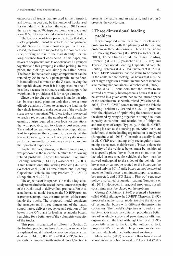
is based on the model of Chen et al. (1995) for the 3D-BPP. However, the proposed model differs from the model of Chen et al. (1995) in several points. First, the objective function has one extra part that represents the sum of the coordinates of the boxes over the vehicle sides. The intention is to minimize the unused space in such a way that the final arrangement is more compact, seeking for a better use of the space in the cargo compartment, providing greater security to the load and preventing boxes to be left without any support.

Another problem found in Chen et al. (1995) can be seen in the arrangement of Figure 1 for a scenario with six boxes where two boxes have no support area. This support area could be the floor of the cargo compartment or the top face of another box. Also the arrangement shown in Figure 1 does not take into consideration the order of unloading the vehicle, which, in practice, leads to a mandatory relocation of boxes each time a new client is visited. For the representation of Figure 1 and the analysis of the model’s results, it was defined that the boxes of the same color belong to the same customer and the unloading sequence goes from the clearer boxes, the white ones, to the darker boxes, the black ones.

A mathematical model to optimize... 353

In this scenario, the darker (black) boxes blocks the removal of the white and grey boxes, the firsts to be unloaded.

The proposed model solves problems with a heterogeneous fleet; in other words, the fleet can be composed of trucks that have different dimensions of the cargo compartment, length, width and height. The model also solves problems when the boxes that will be stowed in the truck have different dimensions, length, width and height. The model assumes that the dimensions of the vehicle, the dimensions of the boxes to be transported and the sequence of the delivery points of the route are all known.

In addition, the proposed model satisfies the following constraints: 1) the volumetric capacity

of each vehicle must not be exceeded; 2) It is not allowed to overlap boxes; 3) the position of the boxes must always be orthogonal to the sides of the compartment; 4) LIFO policy must be respected; and 5) load stability, guaranteed by the support area during transport, must be ensured. The constraints mentioned above make the model closer to the reality of the analyzed company and also makes the model applicable to a wide range of transport companies that transport rectangular boxes. In addition, the model allows boxes to be rotated 90° in X-Y axis. The sets, parameters, decision variables, objective function and constraints of the proposed model are listed next.

Figure 1. Solution from original model solution of Chen et al. (1995).

Sets

C Set of boxes i, ranging from 1 a nn;

D Set of vehicles j, ranging from 1 a nm;

Parameters

nn Number of boxes to be loaded;

nm Number of available vehicles;

M A big number used to the model’s logic;

m A small number used to the model’s logic;

as Support area to be considered in the model, can assume values between 0 and 1, where 0 provides 0% of support area and grows gradually to 1 that guarantees 100% of support area for the box;

oi Indicates the delivery sequence of box i. The box with the lowest value will be visited first and the box with the highest value will be the last to be visited;

pi, qi, ri Length, width and height of box i;

Lj, Wj, Hj Length, width and height of the compartment of vehicle j;

ϕj Cost of each m3 of the vehicle’s j compartment;

w Weight factor for the second part of the objective function.

Pedruzzi, S. et al.354 Gest. Prod., São Carlos, v. 23, n. 2, p. 350-364, 2016

Decision Variables

xi, yi, zi Coordinates of the lower left front corner of box i;

lxi, lyi, lzi Define if the length of box i is parallel to the X, Y or Z axis. For example, lxi is equal to 1 if the length of box i is parallel to X axis, otherwise, lxi is equal to 0;

wxi, wyi, wzi Define if the width of box i is parallel to the X, Y or Z axis. For example, wxi is equal to 1 if the width of box i is parallel to X axis, otherwise, wxi is equal to 0;

hxi, hyi, hzi Define if the height of box i is parallel to the X, Y or Z axis. For example, hxi is equal to 1 if the height of box i is parallel to X axis, otherwise, hxi is equal to 0;

sij Binary variable which indicates if box i is placed in the vehicle j. It is equal to 1 if box i has been placed in the vehicle j and 0 otherwise;

nj Binary variable which indicates if vehicle j was used. It is equal to 1 if vehicle j was used and 0 otherwise;

dikj Binary variable which indicates if box i and box k are placed in the vehicle j. It is equal to 0 if box i and box k are placed in the vehicle j and 1 otherwise;

aik, bik, cik, dik, eik, fik Binary variables that indicate the relative position between two boxes. Variable aik is equal to 1 if the box i is to the left of box k. Similarly, variables bik, cik, dik, eik, fik indicate whether the box i is to the right, behind, ahead, below or above box k, respectively. These variables are necessary only when i ≠ k.

Objective Function

( ) j j j j j i i i ij i i ij D i C i C i C i C

Minimizar L W H n p q r s z x y∈ ∈ ∈ ∈ ∈

− + + + ∑ ∑ ∑ ∑ ∑ϕ w

(1)

Constraints

( ) ( ) ( ) 1 1 i i i i i i i i i i i i ikj k ikx p lx q lz wy hz r lx lz wy hz M x a M+ + − + + − − + − − ≤ + −d , :i k C i k∀ ∈ ≠ (2)

( ) ( ) ( ) 1 1 k k k k k k k k k k k k ikj i ikx p lx q lz wy hz r lx lz wy hz M x b M+ + − + + − − + − − ≤ + −d , :i k C i k∀ ∈ ≠ (3)

( ) ( ) ( ) 1 1 i i i i i i i i i i ikj k iky q wy p lx lz r lx lz wy M y c M+ + − − + + − − ≤ + −d

, :i k C i k∀ ∈ ≠ (4)

( ) ( ) ( ) 1 1 k k k k k k k k k k ikj i iky q wy p lx lz r lx lz wy M y d M+ + − − + + − − ≤ + −d

, :i k C i k∀ ∈ ≠ (5)

( ) ( ) 1 1 i i i i i i i i ikj k ikz r hz q lz hz p lz M z e M+ + − − + − ≤ + −d

, :i k C i k∀ ∈ ≠ (6)

( ) ( ) 1 1 k k k k k k k k ikj i ikz r hz q lz hz p lz M z f M+ + − − + − ≤ + −d , :i k C i k∀ ∈ ≠ (7)

1 ik ik ik ik ik ik ikja b c d e f+ + + + + ≥ −d , : ; i k C i k∀ ∈ ≠ j D∈ (8)

1 ijj D

s∈

=∑ i C∀ ∈ (9)

ij ji C

s M n∈

≤∑

j D∀ ∈ (10)

( ) ( ) ( ). . . 1 1 i i i i i i i i i i i i j ijx p lx q lz wy hz r lx lz wy hz L s M+ + − + + − − + − ≤ + −

, i C j D∀ ∈ ∈ (11)

( ) ( ) ( ) 1 1 i i i i i i i i i i j ijy q wy p lx lz r lx lz wy W s M+ + − − + + − ≤ + −

, i C j D∀ ∈ ∈ (12)

A mathematical model to optimize... 355

small amount to give less weight to this part in the objective function. It was adopted ω = 0.001.

Constraints (2) to (7) ensure that if two boxes are inside the same vehicle, box i cannot overlap box k in any side, or above, or below it. Constraints (8) ensure that if boxes i and box k are in the same vehicle, they must have at least one relative position between each other. Thus, one or more variables bik, cik, dik, eik, fik, must be equal or greater than zero. The left side of Constraints (8) is equal or greater than 1 if the two boxes are in the same vehicle and 0 otherwise.

Constraints (9) ensure that each box must be placed inside only one vehicle. Constraints (10) ensure that if any box is placed in a vehicle, then this vehicle is considered used. Constraints (11) to (13) ensure that all boxes placed in a vehicle can fit in the physical dimensions of the vehicle. Constraints (14) to (19) ensure that the dimensions of a box (length, width and height) must be parallel to one side of the vehicle compartment. Constraints (20) and (21) together define that variable dikj assumes value 0 if the boxes i and k are inside the same vehicle j, and 1 otherwise. Constraints (22) define that all boxes coordinates must be equal or greater than zero. Constraints (23) to (26) define the binary variables of the model.

The objective function, Equation 1, is divided in two parts. The first part aims to reduce the unoccupied volume in all vehicle compartments. The unoccupied volume of the vehicle compartment is calculated as the total volume of the vehicle compartment minus the total volume of the boxes placed in the compartment. The unoccupied volume of the compartment is multiplied by the cost of each m3 of the compartment of vehicle j. Then, this parameter is calculated in preprocessing as j j j / ϕ = β γ . Where

jβ is the cost of the total volume of the compartment of the vehicle and j γ is the volumetric capacity of the vehicle´s compartment.

The second part aims to minimize the sum of the coordinates x, y and z, seeking to reach a more compact arrangement of the boxes. Moreover, this part avoids stowing boxes without touching the compartment floor or without touching the top face of other boxes below and by its side. This part of the objective function makes the boxes arrangement more realistic than the one made by the model of Chen et al. (1995) that leaves boxes without any support beneath them. This second part of the objective function is multiplied by the parameter ω which is a

( ) ( ) 1 1 i i i i i i i i j ijz r hz q lz hz p lz H s M+ + − − + ≤ + −

, i C j D∀ ∈ ∈ (13)

1i i ilx ly lz+ + = i C∀ ∈ (14)

1i i iwx wy wz+ + = i C∀ ∈ (15)

1i i ihx hy hz+ + = i C∀ ∈ (16)

1i i ilx wx hx+ + = i C∀ ∈ (17)

1i i ily wy hy+ + = i C∀ ∈ (18)

1i i ilz wz hz+ + = i C∀ ∈ (19)

2 ij kj ikjs s m− − ≥ d , , i k C j D∀ ∈ ∈ (20)

2 ij kj ikjs s M− − ≤ d , , i k C j D∀ ∈ ∈ (21)

, , 0i i ix y z ≥ i C∀ ∈ (22)

{ }, , , , , , , , , 0,1 i i i i i i i i i ilx ly lz wx wy wz hx hy hz n ∈ i C∀ ∈ (23)

{ }0,1 ijs ∈ , i C j D∀ ∈ ∈ (24)

{ } , , , , , 0,1 ik ik ik ik ik ika b c d e f ∈ , i k C∀ ∈ (25)

{ }0,1 ikj ∈d , , i k C j D∀ ∈ ∈ (26)

Pedruzzi, S. et al.356 Gest. Prod., São Carlos, v. 23, n. 2, p. 350-364, 2016

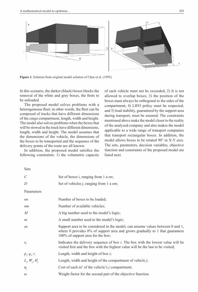
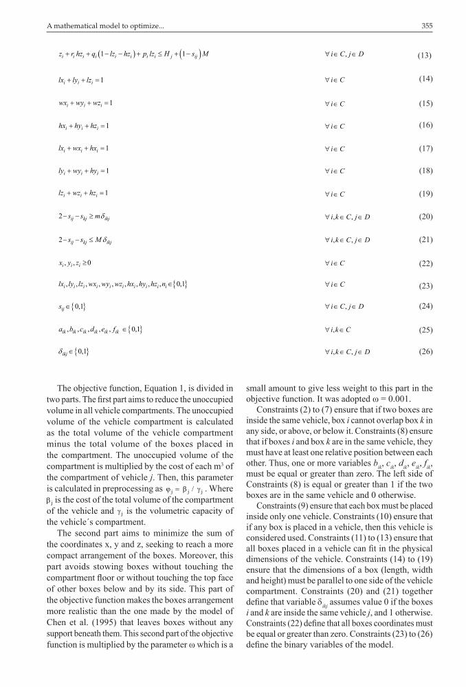
It may be noted from Figure 2 that the solution of the mathematical model reached after the insertion of the Constraints (27) to (31) was satisfactory, but it still does not fully respect the support area issues.

Although in Figure 2 all the boxes are placed on top of another box, the area of the box at the

Constraints (27) ensure that each box has its sides parallel to the sides of the vehicle compartment. Constraints (28) to (30) ensure the reciprocal positioning of boxes, i.e., if box i is to the left of the

box j, necessarily, box j must be to the right of box i. Constraints (31) are inserted to ensure that all boxes will be rotated only in the X-Y plane and then all the boxes will have their heights parallel to the axis Z.

Figure 2. Solution without the restrictions of LIFO and Support Area.

3i i i i i i i i ilx ly lz wx wy wz hx hy hz+ + + + + + + + = i C∀ ∈ (27)

ik kia b= , : i k C i k∀ ∈ ≠ (28)

ik kic d= , :i k C i k∀ ∈ ≠ (29)

ik kie f= , :i k C i k∀ ∈ ≠ (30)

1zih = i C∀ ∈ (31)

bottom is smaller than the area of the box at the top, thereby the box on top is in an unstable situation due to lack of support area. Moreover, it is not yet respected the LIFO policy. Constraints (32) to (35) were proposed to ensure the LIFO policy and, thus, avoid blockages.

( )1 i ik kx c M x+ − ≥ , : ; i ki k C i k o o∀ ∈ ≠ < (32)

( ) ( ) ( ) 1 1 1i i i i i ik k k k k kx p lx q lx c M x p lx q lx+ + − + − ≥ + + − , : ; ; i ki k C i k o o∀ ∈ ≠ < (33)

( )1 i ik kz e M z+ − ≥ , : ; i ki k C i k o o∀ ∈ ≠ < (34)

( )1 i i ik k kz r e M z r+ + − ≥ +

, : ; i ki k C i k o o∀ ∈ ≠ < (35)

Constraints (32) and (33) ensure that the vehicle unloading operation, along the X axis, must respect the LIFO policy, which means that the last boxes loaded on the vehicle will be the first to be unloaded. This ensures that customers are served according to

the established sequence on the route without the need to shift boxes to reach the box to be unloaded in every delivery. Similarly, Constraints (34) and (35) ensure the LIFO order of unloading for the Z axis. This prevents other boxes, that are going to be

A mathematical model to optimize... 357

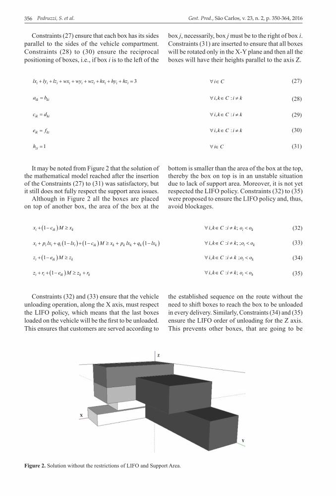
delivered later, be placed on top of the ones that are going to be delivered first. With the inclusion of these constraints, the mathematical model ensures the LIFO policy, as shown in Figure 3.

However, up to this point, the model does not ensure the support area for the boxes. Then, Constraints (36) to (39) are added to the mathematical model to ensure that the boxes will have a support area.

Figure 3. Solution with LIFO policy.

( ) ( ) 1 1 i i i i i ik kx p lx q lx e M x+ + − + − ≥ , : i k C i k∀ ∈ ≠ (36)

( ) ( ) ( ) 1 1 ( 1 ) i i i i i k ik k k k kx p lx q lx x e M p lx q lx as+ + − − + − ≥ + − , : i k C i k∀ ∈ ≠ (37)

( ) ( ) 1 1 i i i i i ik ky p ly q ly e M y+ + − + − ≥ , : i k C i k∀ ∈ ≠ (38)

( ) ( ) ( ) 1 1 ( 1 ) i i i i i k ik k k k ky p ly q ly y e M p ly q ly as+ + − − + − ≥ + − , : i k C i k∀ ∈ ≠ (39)

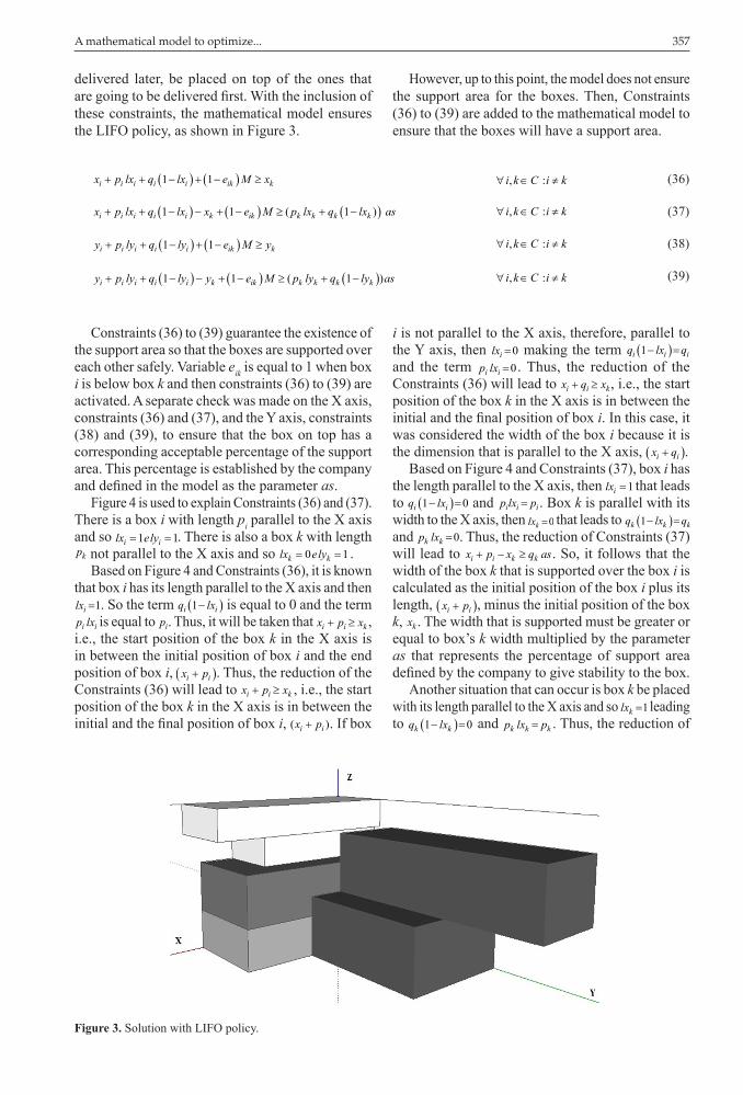
Constraints (36) to (39) guarantee the existence of the support area so that the boxes are supported over each other safely. Variable eik is equal to 1 when box i is below box k and then constraints (36) to (39) are activated. A separate check was made on the X axis, constraints (36) and (37), and the Y axis, constraints (38) and (39), to ensure that the box on top has a corresponding acceptable percentage of the support area. This percentage is established by the company and defined in the model as the parameter as.

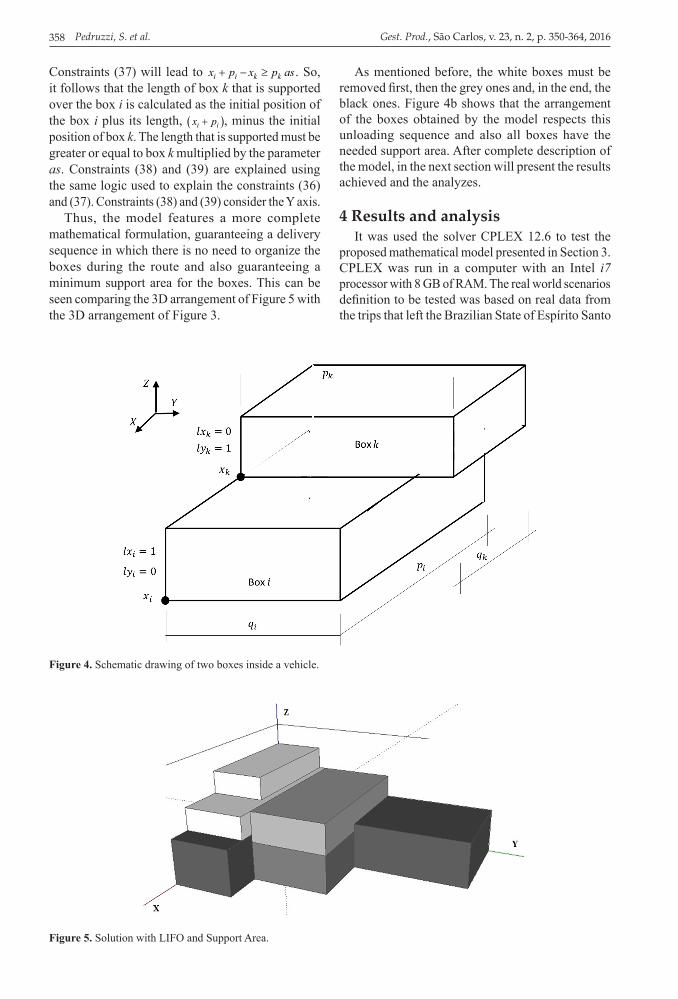
Figure 4 is used to explain Constraints (36) and (37). There is a box i with length pi parallel to the X axis and so 1 1i ilx ely= = . There is also a box k with length

kp not parallel to the X axis and so 0 1k klx ely= = .Based on Figure 4 and Constraints (36), it is known

that box i has its length parallel to the X axis and then 1 ilx = . So the term ( ) 1i iq lx− is equal to 0 and the term i ip lx is equal to ip . Thus, it will be taken that i i kx p x+ ≥ ,

i.e., the start position of the box k in the X axis is in between the initial position of box i and the end position of box i, ( )i ix p+ . Thus, the reduction of the Constraints (36) will lead to i i kx p x+ ≥ , i.e., the start position of the box k in the X axis is in between the initial and the final position of box i, ( )i ix p+ . If box

i is not parallel to the X axis, therefore, parallel to the Y axis, then 0ilx = making the term ( ) 1 i i iq lx q− = and the term 0i ip lx = . Thus, the reduction of the Constraints (36) will lead to i i kx q x+ ≥ , i.e., the start position of the box k in the X axis is in between the initial and the final position of box i. In this case, it was considered the width of the box i because it is the dimension that is parallel to the X axis, ( )i ix q+ .

Based on Figure 4 and Constraints (37), box i has the length parallel to the X axis, then 1ilx = that leads to ( )1 0i iq lx− = and i i ip lx p= . Box k is parallel with its width to the X axis, then 0klx = that leads to ( ) 1 k k kq lx q− = and 0k kp lx = . Thus, the reduction of Constraints (37) will lead to i i k kx p x q as+ − ≥ . So, it follows that the width of the box k that is supported over the box i is calculated as the initial position of the box i plus its length, ( )i ix p+ , minus the initial position of the box k, kx . The width that is supported must be greater or equal to box’s k width multiplied by the parameter as that represents the percentage of support area defined by the company to give stability to the box.

Another situation that can occur is box k be placed with its length parallel to the X axis and so 1 klx = leading to ( ) 1 0k kq lx− = and k k kp lx p= . Thus, the reduction of

Pedruzzi, S. et al.358 Gest. Prod., São Carlos, v. 23, n. 2, p. 350-364, 2016

Constraints (37) will lead to i i k kx p x p as+ − ≥ . So, it follows that the length of box k that is supported over the box i is calculated as the initial position of the box i plus its length, ( )i ix p+ , minus the initial position of box k. The length that is supported must be greater or equal to box k multiplied by the parameter as. Constraints (38) and (39) are explained using the same logic used to explain the constraints (36) and (37). Constraints (38) and (39) consider the Y axis.

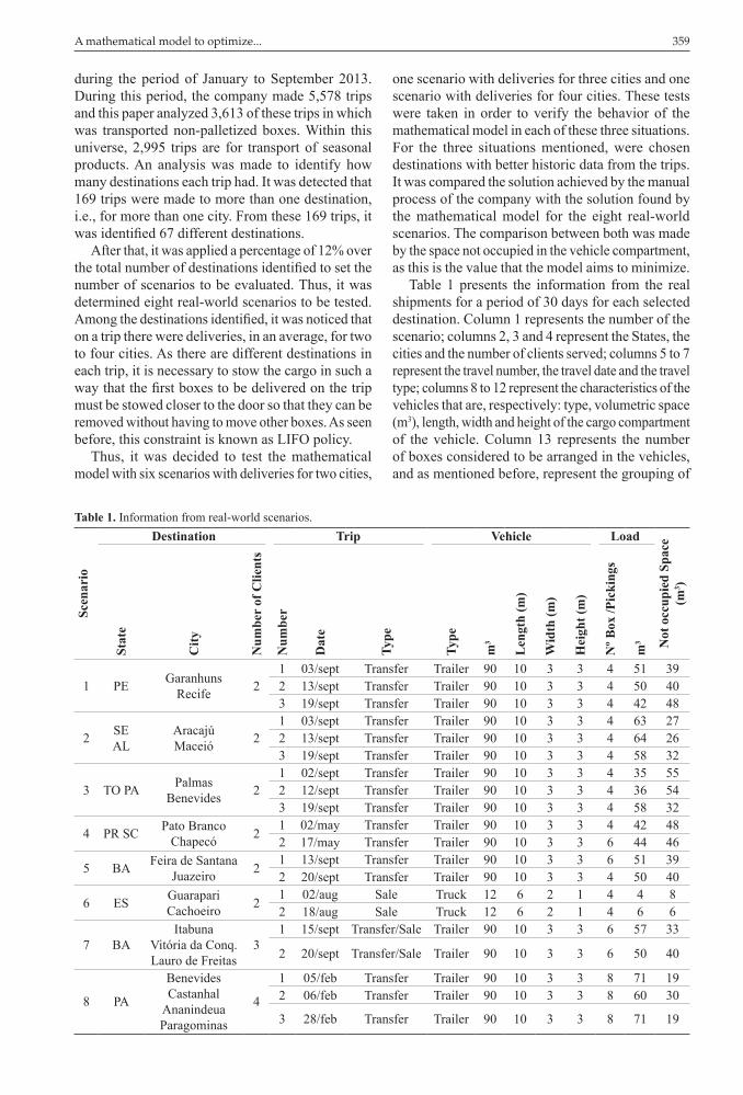
Thus, the model features a more complete mathematical formulation, guaranteeing a delivery sequence in which there is no need to organize the boxes during the route and also guaranteeing a minimum support area for the boxes. This can be seen comparing the 3D arrangement of Figure 5 with the 3D arrangement of Figure 3.

As mentioned before, the white boxes must be removed first, then the grey ones and, in the end, the black ones. Figure 4b shows that the arrangement of the boxes obtained by the model respects this unloading sequence and also all boxes have the needed support area. After complete description of the model, in the next section will present the results achieved and the analyzes.

4 Results and analysisIt was used the solver CPLEX 12.6 to test the

proposed mathematical model presented in Section 3. CPLEX was run in a computer with an Intel i7 processor with 8 GB of RAM. The real world scenarios definition to be tested was based on real data from the trips that left the Brazilian State of Espírito Santo

Figure 5. Solution with LIFO and Support Area.

Figure 4. Schematic drawing of two boxes inside a vehicle.

A mathematical model to optimize... 359

during the period of January to September 2013. During this period, the company made 5,578 trips and this paper analyzed 3,613 of these trips in which was transported non-palletized boxes. Within this universe, 2,995 trips are for transport of seasonal products. An analysis was made to identify how many destinations each trip had. It was detected that 169 trips were made to more than one destination, i.e., for more than one city. From these 169 trips, it was identified 67 different destinations.

After that, it was applied a percentage of 12% over the total number of destinations identified to set the number of scenarios to be evaluated. Thus, it was determined eight real-world scenarios to be tested. Among the destinations identified, it was noticed that on a trip there were deliveries, in an average, for two to four cities. As there are different destinations in each trip, it is necessary to stow the cargo in such a way that the first boxes to be delivered on the trip must be stowed closer to the door so that they can be removed without having to move other boxes. As seen before, this constraint is known as LIFO policy.

Thus, it was decided to test the mathematical model with six scenarios with deliveries for two cities,

one scenario with deliveries for three cities and one scenario with deliveries for four cities. These tests were taken in order to verify the behavior of the mathematical model in each of these three situations. For the three situations mentioned, were chosen destinations with better historic data from the trips. It was compared the solution achieved by the manual process of the company with the solution found by the mathematical model for the eight real-world scenarios. The comparison between both was made by the space not occupied in the vehicle compartment, as this is the value that the model aims to minimize.

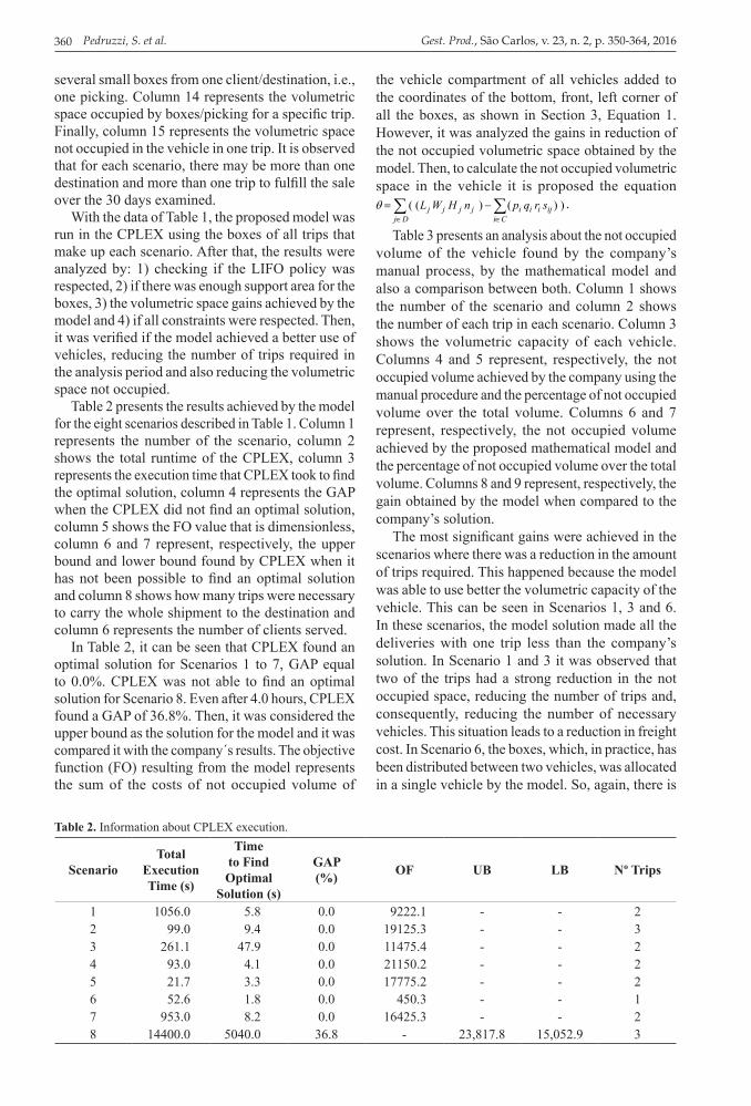
Table 1 presents the information from the real shipments for a period of 30 days for each selected destination. Column 1 represents the number of the scenario; columns 2, 3 and 4 represent the States, the cities and the number of clients served; columns 5 to 7 represent the travel number, the travel date and the travel type; columns 8 to 12 represent the characteristics of the vehicles that are, respectively: type, volumetric space (m3), length, width and height of the cargo compartment of the vehicle. Column 13 represents the number of boxes considered to be arranged in the vehicles, and as mentioned before, represent the grouping of

Table 1. Information from real-world scenarios.

Scen

ario

Destination Trip Vehicle Load

Not

occ

upie

d Sp

ace

(m3 )

Stat

e

City

Num

ber

of C

lient

s

Num

ber

Dat

e

Type

Type

m3

Len

gth

(m)

Wid

th (m

)

Hei

ght (

m)

Nº B

ox /P

icki

ngs

m3

1 PE Garanhuns Recife 2

1 03/sept Transfer Trailer 90 10 3 3 4 51 392 13/sept Transfer Trailer 90 10 3 3 4 50 403 19/sept Transfer Trailer 90 10 3 3 4 42 48

2 SE AL

Aracajú Maceió 2

1 03/sept Transfer Trailer 90 10 3 3 4 63 272 13/sept Transfer Trailer 90 10 3 3 4 64 263 19/sept Transfer Trailer 90 10 3 3 4 58 32

3 TO PA Palmas Benevides 2

1 02/sept Transfer Trailer 90 10 3 3 4 35 552 12/sept Transfer Trailer 90 10 3 3 4 36 543 19/sept Transfer Trailer 90 10 3 3 4 58 32

4 PR SC Pato Branco Chapecó 2

1 02/may Transfer Trailer 90 10 3 3 4 42 482 17/may Transfer Trailer 90 10 3 3 6 44 46

5 BA Feira de Santana Juazeiro 2

1 13/sept Transfer Trailer 90 10 3 3 6 51 392 20/sept Transfer Trailer 90 10 3 3 4 50 40

6 ES Guarapari Cachoeiro 2

1 02/aug Sale Truck 12 6 2 1 4 4 82 18/aug Sale Truck 12 6 2 1 4 6 6

7 BAItabuna

Vitória da Conq. Lauro de Freitas

31 15/sept Transfer/Sale Trailer 90 10 3 3 6 57 33

2 20/sept Transfer/Sale Trailer 90 10 3 3 6 50 40

8 PA

Benevides Castanhal

Ananindeua Paragominas

4

1 05/feb Transfer Trailer 90 10 3 3 8 71 192 06/feb Transfer Trailer 90 10 3 3 8 60 30

3 28/feb Transfer Trailer 90 10 3 3 8 71 19

Pedruzzi, S. et al.360 Gest. Prod., São Carlos, v. 23, n. 2, p. 350-364, 2016

several small boxes from one client/destination, i.e., one picking. Column 14 represents the volumetric space occupied by boxes/picking for a specific trip. Finally, column 15 represents the volumetric space not occupied in the vehicle in one trip. It is observed that for each scenario, there may be more than one destination and more than one trip to fulfill the sale over the 30 days examined.

With the data of Table 1, the proposed model was run in the CPLEX using the boxes of all trips that make up each scenario. After that, the results were analyzed by: 1) checking if the LIFO policy was respected, 2) if there was enough support area for the boxes, 3) the volumetric space gains achieved by the model and 4) if all constraints were respected. Then, it was verified if the model achieved a better use of vehicles, reducing the number of trips required in the analysis period and also reducing the volumetric space not occupied.

Table 2 presents the results achieved by the model for the eight scenarios described in Table 1. Column 1 represents the number of the scenario, column 2 shows the total runtime of the CPLEX, column 3 represents the execution time that CPLEX took to find the optimal solution, column 4 represents the GAP when the CPLEX did not find an optimal solution, column 5 shows the FO value that is dimensionless, column 6 and 7 represent, respectively, the upper bound and lower bound found by CPLEX when it has not been possible to find an optimal solution and column 8 shows how many trips were necessary to carry the whole shipment to the destination and column 6 represents the number of clients served.

In Table 2, it can be seen that CPLEX found an optimal solution for Scenarios 1 to 7, GAP equal to 0.0%. CPLEX was not able to find an optimal solution for Scenario 8. Even after 4.0 hours, CPLEX found a GAP of 36.8%. Then, it was considered the upper bound as the solution for the model and it was compared it with the company´s results. The objective function (FO) resulting from the model represents the sum of the costs of not occupied volume of

the vehicle compartment of all vehicles added to the coordinates of the bottom, front, left corner of all the boxes, as shown in Section 3, Equation 1. However, it was analyzed the gains in reduction of the not occupied volumetric space obtained by the model. Then, to calculate the not occupied volumetric space in the vehicle it is proposed the equation

( ( ) ( ) )j j j j i i i ijj D i C

L W H n p q r s∈ ∈

= −∑ ∑θ .

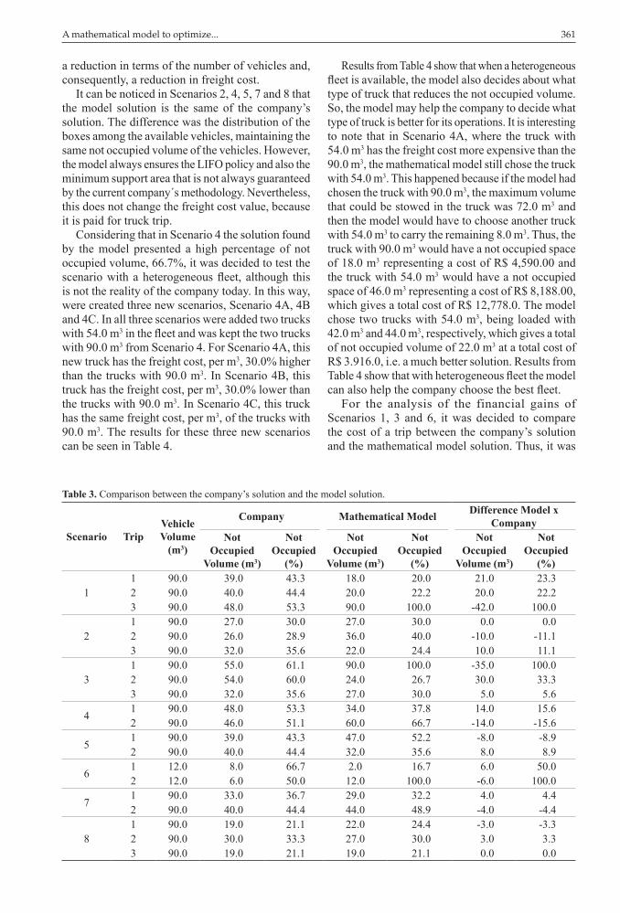
Table 3 presents an analysis about the not occupied volume of the vehicle found by the company’s manual process, by the mathematical model and also a comparison between both. Column 1 shows the number of the scenario and column 2 shows the number of each trip in each scenario. Column 3 shows the volumetric capacity of each vehicle. Columns 4 and 5 represent, respectively, the not occupied volume achieved by the company using the manual procedure and the percentage of not occupied volume over the total volume. Columns 6 and 7 represent, respectively, the not occupied volume achieved by the proposed mathematical model and the percentage of not occupied volume over the total volume. Columns 8 and 9 represent, respectively, the gain obtained by the model when compared to the company’s solution.

The most significant gains were achieved in the scenarios where there was a reduction in the amount of trips required. This happened because the model was able to use better the volumetric capacity of the vehicle. This can be seen in Scenarios 1, 3 and 6. In these scenarios, the model solution made all the deliveries with one trip less than the company’s solution. In Scenario 1 and 3 it was observed that two of the trips had a strong reduction in the not occupied space, reducing the number of trips and, consequently, reducing the number of necessary vehicles. This situation leads to a reduction in freight cost. In Scenario 6, the boxes, which, in practice, has been distributed between two vehicles, was allocated in a single vehicle by the model. So, again, there is

Table 2. Information about CPLEX execution.

ScenarioTotal

Execution Time (s)

Time to Find Optimal

Solution (s)

GAP (%) OF UB LB Nº Trips

1 1056.0 5.8 0.0 9222.1 - - 22 99.0 9.4 0.0 19125.3 - - 33 261.1 47.9 0.0 11475.4 - - 24 93.0 4.1 0.0 21150.2 - - 25 21.7 3.3 0.0 17775.2 - - 26 52.6 1.8 0.0 450.3 - - 17 953.0 8.2 0.0 16425.3 - - 28 14400.0 5040.0 36.8 - 23,817.8 15,052.9 3

A mathematical model to optimize... 361

a reduction in terms of the number of vehicles and, consequently, a reduction in freight cost.

It can be noticed in Scenarios 2, 4, 5, 7 and 8 that the model solution is the same of the company’s solution. The difference was the distribution of the boxes among the available vehicles, maintaining the same not occupied volume of the vehicles. However, the model always ensures the LIFO policy and also the minimum support area that is not always guaranteed by the current company´s methodology. Nevertheless, this does not change the freight cost value, because it is paid for truck trip.

Considering that in Scenario 4 the solution found by the model presented a high percentage of not occupied volume, 66.7%, it was decided to test the scenario with a heterogeneous fleet, although this is not the reality of the company today. In this way, were created three new scenarios, Scenario 4A, 4B and 4C. In all three scenarios were added two trucks with 54.0 m3 in the fleet and was kept the two trucks with 90.0 m3 from Scenario 4. For Scenario 4A, this new truck has the freight cost, per m3, 30.0% higher than the trucks with 90.0 m3. In Scenario 4B, this truck has the freight cost, per m3, 30.0% lower than the trucks with 90.0 m3. In Scenario 4C, this truck has the same freight cost, per m3, of the trucks with 90.0 m3. The results for these three new scenarios can be seen in Table 4.

Results from Table 4 show that when a heterogeneous fleet is available, the model also decides about what type of truck that reduces the not occupied volume. So, the model may help the company to decide what type of truck is better for its operations. It is interesting to note that in Scenario 4A, where the truck with 54.0 m3 has the freight cost more expensive than the 90.0 m3, the mathematical model still chose the truck with 54.0 m3. This happened because if the model had chosen the truck with 90.0 m3, the maximum volume that could be stowed in the truck was 72.0 m3 and then the model would have to choose another truck with 54.0 m3 to carry the remaining 8.0 m3. Thus, the truck with 90.0 m3 would have a not occupied space of 18.0 m3 representing a cost of R$ 4,590.00 and the truck with 54.0 m3 would have a not occupied space of 46.0 m3 representing a cost of R$ 8,188.00, which gives a total cost of R$ 12,778.0. The model chose two trucks with 54.0 m3, being loaded with 42.0 m3 and 44.0 m3, respectively, which gives a total of not occupied volume of 22.0 m3 at a total cost of R$ 3.916.0, i.e. a much better solution. Results from Table 4 show that with heterogeneous fleet the model can also help the company choose the best fleet.

For the analysis of the financial gains of Scenarios 1, 3 and 6, it was decided to compare the cost of a trip between the company’s solution and the mathematical model solution. Thus, it was

Table 3. Comparison between the company’s solution and the model solution.

Scenario TripVehicle Volume

(m3)

Company Mathematical Model Difference Model x Company

Not Occupied

Volume (m3)

Not Occupied

(%)

Not Occupied

Volume (m3)

Not Occupied

(%)

Not Occupied

Volume (m3)

Not Occupied

(%)

11 90.0 39.0 43.3 18.0 20.0 21.0 23.32 90.0 40.0 44.4 20.0 22.2 20.0 22.23 90.0 48.0 53.3 90.0 100.0 -42.0 100.0

21 90.0 27.0 30.0 27.0 30.0 0.0 0.02 90.0 26.0 28.9 36.0 40.0 -10.0 -11.13 90.0 32.0 35.6 22.0 24.4 10.0 11.1

31 90.0 55.0 61.1 90.0 100.0 -35.0 100.02 90.0 54.0 60.0 24.0 26.7 30.0 33.33 90.0 32.0 35.6 27.0 30.0 5.0 5.6

41 90.0 48.0 53.3 34.0 37.8 14.0 15.62 90.0 46.0 51.1 60.0 66.7 -14.0 -15.6

51 90.0 39.0 43.3 47.0 52.2 -8.0 -8.92 90.0 40.0 44.4 32.0 35.6 8.0 8.9

61 12.0 8.0 66.7 2.0 16.7 6.0 50.02 12.0 6.0 50.0 12.0 100.0 -6.0 100.0

71 90.0 33.0 36.7 29.0 32.2 4.0 4.42 90.0 40.0 44.4 44.0 48.9 -4.0 -4.4

81 90.0 19.0 21.1 22.0 24.4 -3.0 -3.32 90.0 30.0 33.3 27.0 30.0 3.0 3.33 90.0 19.0 21.1 19.0 21.1 0.0 0.0

Pedruzzi, S. et al.362 Gest. Prod., São Carlos, v. 23, n. 2, p. 350-364, 2016

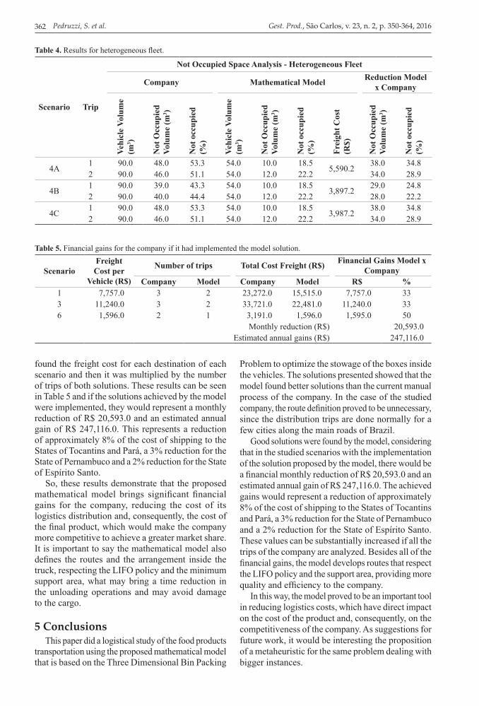
found the freight cost for each destination of each scenario and then it was multiplied by the number of trips of both solutions. These results can be seen in Table 5 and if the solutions achieved by the model were implemented, they would represent a monthly reduction of R$ 20,593.0 and an estimated annual gain of R$ 247,116.0. This represents a reduction of approximately 8% of the cost of shipping to the States of Tocantins and Pará, a 3% reduction for the State of Pernambuco and a 2% reduction for the State of Espírito Santo.

So, these results demonstrate that the proposed mathematical model brings significant financial gains for the company, reducing the cost of its logistics distribution and, consequently, the cost of the final product, which would make the company more competitive to achieve a greater market share. It is important to say the mathematical model also defines the routes and the arrangement inside the truck, respecting the LIFO policy and the minimum support area, what may bring a time reduction in the unloading operations and may avoid damage to the cargo.

5 ConclusionsThis paper did a logistical study of the food products

transportation using the proposed mathematical model that is based on the Three Dimensional Bin Packing

Problem to optimize the stowage of the boxes inside the vehicles. The solutions presented showed that the model found better solutions than the current manual process of the company. In the case of the studied company, the route definition proved to be unnecessary, since the distribution trips are done normally for a few cities along the main roads of Brazil.

Good solutions were found by the model, considering that in the studied scenarios with the implementation of the solution proposed by the model, there would be a financial monthly reduction of R$ 20,593.0 and an estimated annual gain of R$ 247,116.0. The achieved gains would represent a reduction of approximately 8% of the cost of shipping to the States of Tocantins and Pará, a 3% reduction for the State of Pernambuco and a 2% reduction for the State of Espírito Santo. These values can be substantially increased if all the trips of the company are analyzed. Besides all of the financial gains, the model develops routes that respect the LIFO policy and the support area, providing more quality and efficiency to the company.

In this way, the model proved to be an important tool in reducing logistics costs, which have direct impact on the cost of the product and, consequently, on the competitiveness of the company. As suggestions for future work, it would be interesting the proposition of a metaheuristic for the same problem dealing with bigger instances.

Table 5. Financial gains for the company if it had implemented the model solution.

ScenarioFreight Cost per

Vehicle (R$)

Number of trips Total Cost Freight (R$) Financial Gains Model x Company

Company Model Company Model R$ %1 7,757.0 3 2 23,272.0 15,515.0 7,757.0 333 11,240.0 3 2 33,721.0 22,481.0 11,240.0 336 1,596.0 2 1 3,191.0 1,596.0 1,595.0 50

Monthly reduction (R$) 20,593.0Estimated annual gains (R$) 247,116.0

Table 4. Results for heterogeneous fleet.

Scenario Trip

Not Occupied Space Analysis - Heterogeneous Fleet

Company Mathematical Model Reduction Model x Company

Vehi

cle

Volu

me

(m3 )

Not

Occ

upie

d Vo

lum

e (m

3 )

Not

occ

upie

d (%

)

Vehi

cle

Volu

me

(m3 )

Not

Occ

upie

d Vo

lum

e (m

3 )

Not

occ

upie

d (%

)

Frei

ght C

ost

(R$)

Not

Occ

upie

d Vo

lum

e (m

3 )

Not

occ

upie

d (%

)

4A1 90.0 48.0 53.3 54.0 10.0 18.5

5,590.238.0 34.8

2 90.0 46.0 51.1 54.0 12.0 22.2 34.0 28.9

4B1 90.0 39.0 43.3 54.0 10.0 18.5

3,897.229.0 24.8

2 90.0 40.0 44.4 54.0 12.0 22.2 28.0 22.2

4C1 90.0 48.0 53.3 54.0 10.0 18.5

3,987.238.0 34.8

2 90.0 46.0 51.1 54.0 12.0 22.2 34.0 28.9

A mathematical model to optimize... 363

AcknowledgementsThe authors thank the FAPES (458/2013), CNPq

(477357/2013-0) and CAPES for financial support and the studied company by the information and data provided.

ReferencesAraujo, R. R., Michel, F. D., & Senna, L. A. S. (2011).

Uma abordagem de resolução integrada para os problemas de roteirização e carregamento de veículos. In: Confederação Nacional do Transporte – CNT, & Associação Nacional de Pesquisa e Ensino em Transportes – ANPET. Transporte em transformação XVI: trabalhos vencedores do Prêmio CNT: produção acadêmica 2011. Brasília: Positiva. 216 p.

Attanasio, A., Fuduli, A., Ghiani, G., & Triki, C. (2007). Integrated shipment dispatching and packing problems: a case study. Journal of Mathematical Modelling and Algorithms, 6(1), 77-85. http://dx.doi.org/10.1007/s10852-006-9050-5.

Bortfeldt, A., & Homberger, J. (2013). Packing first, routing second - a heuristic for the vehicle routing and loading problem. Computers & Operations Research, 40(3), 873-885. http://dx.doi.org/10.1016/j.cor.2012.09.005.

Bortfeldt, A., & Wäscher, G. (2013). Constraints in container loading – a state-of-the-art review. European Journal of Operational Research, 229(1), 1-20. http://dx.doi.org/10.1016/j.ejor.2012.12.006.

Bortfeldt, A., (2012). A hybrid algorithm for the capacitated vehicle routing problem with three dimensional loading constraints. Computers & Operations Research, 39(9), 2248-2257. http://dx.doi.org/10.1016/j.cor.2011.11.008.

Ceschia, S., & Schaerf, A. (2013). Local search for a multi-drop multi-container loading problem. Journal of Heuristics, 19(2), 275-294. http://dx.doi.org/10.1007/s10732-011-9162-6.

Chen, C. S., Lee, S. M., & Shen, Q. S. (1995). An analytical model for the container loading problem. European Journal of Operational Research, 80(1), 68-76. http://dx.doi.org/10.1016/0377-2217(94)00002-T.

Confederação Nacional do Transporte – CNT. (2013). Boletim estatístico – CNT. Recuperado em 17 de fevereiro de 2014, de http:/www.cnt.org.br/

Crainic, T. G., Perboli, G., & Tadei, R. (2009). TS2 PACK: a two-level tabu search for the three-dimensional bin packing problem. European Journal of Operational Research, 195(3), 744-760. http://dx.doi.org/10.1016/j.ejor.2007.06.063.

Crainic, T., Perboli, G., & Tadei, R. (2008). Extreme point-based heuristics for three-dimensional bin packing. INFORMS Journal on Computing, 20(3), 368-384. http://dx.doi.org/10.1287/ijoc.1070.0250.

Den Boef, E., Korst, J., Martello, S., Pisinger, D., & Vigo, D. (2005). Erratum to “the three-dimensional bin packing

problem”: robot-packable and orthogonal variants of packing problems. Operations Research, 53(4), 735-736. http://dx.doi.org/10.1287/opre.1050.0210.

Faroe, O., Pisinger, D., & Zachariasen, M. (2003). Guided local search for three-dimensional bin-packing problem. INFORMS Journal on Computing, 15(3), 267-283. http://dx.doi.org/10.1287/ijoc.15.3.267.16080.

Fuellerer, G., Doerner, K. F., Hartl, R. F., & Iori, M. (2010). Metaheuristics for vehicle routing problems with three-dimensional loading constraints. European Journal of Operational Research, 201(3), 751-759. http://dx.doi.org/10.1016/j.ejor.2009.03.046.

Gendreau, M., Iori, M., Laporte, G., & Martello, S. (2006). A tabu search algorithm for a routing and container loading problem. Transportation Science, 40(3), 342-350. http://dx.doi.org/10.1287/trsc.1050.0145.

George, J., & Robinson, D. (1980). A heuristic for packing boxes into a container. Computers & Operations Research, 7(3), 147-156. http://dx.doi.org/10.1016/0305-0548(80)90001-5.

Iori, M., & Martello, S. (2010). Routing problems with loading constraints. Top (Madrid), 18(1), 4-27. http://dx.doi.org/10.1007/s11750-010-0144-x.

Iori, M., & Martello, S. (2013). An annotated bibliography of combined routing and loading problems. The Yugoslav Journal of Operations Research, 23(3), 1-16.

Junqueira, L., Morabito, R., & Yamashita, D. (2011). Abordagens para problemas de carregamento de contêineres com considerações de múltiplos destinos. Gestão & Produção, 18(2), 265-284. http://dx.doi.org/10.1590/S0104-530X2011000200004.

Junqueira, L., Oliveira, J. F., Carravilla, M. A., & Morabito, R. (2013). An optimization model for the vehicle routing problem with practical three-dimensional loading constraints. International Transactions in Operational Research, 20(5), 645-666. http://dx.doi.org/10.1111/j.1475-3995.2012.00872.x.

Koloch, G., & Kaminski, B. (2010). Nested vs. joint optimization of vehicle routing problems with three-dimensional loading constraints. Engineering Letters, 18, 193-198.

Lodi, A., Martello, S., & Vigo, D. (2002). Heuristic algorithms for the three-dimensional bin packing problem. European Journal of Operational Research, 141(2), 410-420. http://dx.doi.org/10.1016/S0377-2217(02)00134-0.

Martello, S., Pisinger, D., & Vigo, D. (2000). The three-dimensional bin packing problem. Operations Research, 48(2), 256-257. http://dx.doi.org/10.1287/opre.48.2.256.12386.

Martello, S., Pisinger, D., Vigo, D., Boef, E. D., & Korst, J. (2007). Algorithm 864: general and robot-packable variants of the three-dimensional bin packing problem. ACM Transactions on Mathematical Software, 33(1), 1-12. http://dx.doi.org/10.1145/1206040.1206047.

Pedruzzi, S. et al.364 Gest. Prod., São Carlos, v. 23, n. 2, p. 350-364, 2016

Tarantilis, C. D., Zachariadis, E. E., & Kiranoudis, C. T. (2009). A hybrid metaheuristic algorithm for the integrated vehicle routing and three-dimensional container-loading problem. Transactions on Intelligent Transportation Systems, IEEE, 10(2), 255-271. http://dx.doi.org/10.1109/TITS.2009.2020187.

Wang, Z., Li, K. W., & Levy, J. K. (2008). A heuristic for the container loading problem: a tertiary-tree-based dynamic space decomposition approach. European Journal of Operational Research, 191(1), 86-99. http://dx.doi.org/10.1016/j.ejor.2007.08.017.

Wäscher, G., Haußner, H., & Schumann, H. (2007). An improved typology of cutting and packing problems. European Journal of Operational Research, 183(3), 1109-1130. http://dx.doi.org/10.1016/j.ejor.2005.12.047.

Wu, Y., Li, W., Goh, M., & Souza, R. (2010). Three-dimensional bin packing problem with variable bin height. European Journal of Operational Research, 202(2), 347-355. http://dx.doi.org/10.1016/j.ejor.2009.05.040.

Zhang, D.-F., Wei, L.-J., Chen, Q.-S., & Chen, H.-W. (2007). A combinational heuristic algorithm for the three-dimensional packing problem. Journal of Software, 18(9), 2083-2089. http://dx.doi.org/10.1360/jos182083.

Zhu, W., Qin, H., Lim, A., & Wang, L. (2012). A two-stage tabu search algorithm with enhanced packing heuristics for the 3L-CVRP and M3L-CVRP. Computers & Operations Research, 39(9), 2178-2195. http://dx.doi.org/10.1016/j.cor.2011.11.001.

Moura, A.( 2008). A multi-objective genetic algorithm for the vehicle routing with time windows and loading. In: A. Bortfeldt, J. Homberger, H. Kopfer, G. Pankratz, & R. Strangmeier (Eds.), Intelligent decision support (pp. 187-201). Malsch, Germany: Gabler GmbH & Co.

Moura, A., & Oliveira, J. F. (2009). An integrated approach to vehicle routing and container loading problems. OR-Spektrum, 31(4), 775-800. http://dx.doi.org/10.1007/s00291-008-0129-4.

Peng, Y., Zhang, D., & Chin, F. Y. L. (2009). A hybrid simulated annealing algorithm for container loading problem. In: Proceedings of the 1st ACM/SIGEVO Summit on Genetic and Evolutionary Computation (pp. 919-928). Shanghai: ACM.

Pisinger, D. (2002). Heuristics for the container loading problem. European Journal of Operational Research, 141(2), 382-392. http://dx.doi.org/10.1016/S0377-2217(02)00132-7.

Ruan, Q., Zhang, Z., Miao, L., & Shen, H. (2013). Hybrid approach for the vehicle routing problem with three-dimensional loading constraints. Computers & Operations Research, 40(6), 1579-1589. http://dx.doi.org/10.1016/j.cor.2011.11.013.

Tao, Y., & Wang, F. (2010). A new packing heuristic based algorithm for vehicle routing problem with three-dimensional loading constraints. In: International Conference on Automation Science and Engineering, IEEE, CASE 2010 (pp. 972-977). Toronto: IEEE.