A Generalized Hypergeometric Function II. Asymptotics and ...siru/papers/p61.pdf · Generalized Hypergeometric Function II 391 Finally, the contour C is given by a horizontal line

Digital Object Identifier (DOI) 10.1007/s00220-003-0969-3Commun. Math. Phys. 243, 389–412 (2003) Communications in

MathematicalPhysics

A Generalized Hypergeometric Function II.Asymptotics and D4 Symmetry

S.N.M. Ruijsenaars

Centre for Mathematics and Computer Science, P.O.Box 94079, 1090 GB Amsterdam, The Netherlands

Received: 28 November 2002 / Accepted: 22 May 2003Published online: 11 November 2003 – © Springer-Verlag 2003

Abstract: In previous work we introduced and studied a function R(a+, a−, c; v, v) thatgeneralizes the hypergeometric function. In this paper we focus on a similarity-trans-formed function E(a+, a−, γ ; v, v), with parameters γ ∈ C

4 related to the couplingsc ∈ C

4 by a shift depending on a+, a−. We show that the E-function is invariant underall maps γ �→ w(γ ), with w in the Weyl group of type D4. Choosing a+, a− positiveand γ, v real, we obtain detailed information on the |Re v| → ∞ asymptotics of theE-function. In particular, we explicitly determine the leading asymptotics in terms ofplane waves and the c-function that implements the similarity R → E .

Contents

1. Introduction . . . . . . . . . . . . . . . . . . . . . . . . . . . . . . . . . . 3892. D4-Invariance: First Steps . . . . . . . . . . . . . . . . . . . . . . . . . . . 3953. Asymptotics: The Key Results . . . . . . . . . . . . . . . . . . . . . . . . 3994. Proofs of Theorems 1.1 and 1.2 . . . . . . . . . . . . . . . . . . . . . . . . 406

1. Introduction

This paper may be viewed as a continuation of our previous paper Ref. [1]. The“relativistic” hypergeometric function R(a+, a−, c0, c1, c2, c3; v, v) at issue here wasfirst introduced in Ref. [2], as an eigenfunction of a relativistic Hamiltonian ofCalogero-Moser type. This generalizes the fact that in suitable variables the 2F1-functionis an eigenfunction of a nonrelativistic Hamiltonian of Calogero-Moser type. Likewise,the discretization of 2F1 yielding the Jacobi polynomials generalizes to discretizationsof R yielding the Askey-Wilson polynomials [3, 4]. Our lecture notes [2] and Ref. [1](henceforth referred to as I) contain extensive background material and references torelated work. More recent surveys pertinent to our R-function include Refs. [5, 6].

390 S.N.M. Ruijsenaars

We have occasion to invoke various results from I, some of which we begin by sum-marizing. This summary also serves to collect some definitions and notation from I, withan eye on making this paper and its sequel Ref. [7] somewhat more self-contained.

We begin by recalling how R(a+, a−, c; v, v) is defined via an integral involvingour “hyperbolic gamma function” G(a+, a−; z) as a building block. First, we introducequantities

as ≡ min(a+, a−), al ≡ max(a+, a−), a ≡ (a+ + a−)/2, α ≡ 2π/a+a−, (1.1)

s1 ≡ c0 + c1 − a−/2, s2 ≡ c0 + c2 − a+/2, s3 ≡ c0 + c3, (1.2)

c0 ≡ (c0 + c1 + c2 + c3)/2. (1.3)

Second, we take a+, a− > 0 and c ∈ R4 unless explicitly stated otherwise. To ease

the exposition, we also choose at first Re v and Re v positive and s1, s2, s3 ∈ (−a, a).Then we can define the R-function by the contour integral

R(c; v, v) = 1

(a+a−)1/2

∫C

F(c0; v, z)K(c; z)F (c0; v, z)dz, (1.4)

where

F(b; y, z) ≡ G(z + y + ib − ia)

G(y + ib − ia)

G(z − y + ib − ia)

G(−y + ib − ia), (1.5)

K(c; z) ≡ 1

G(z + ia)

3∏j=1

G(isj )

G(z + isj ). (1.6)

(To unburden the notation, we often suppress the dependence on the parameters a+, a−.)As concerns the G-function occurring in these formulas, we recall from I Appendix A

that it can be written as

G(a+, a−; z) = E(a+, a−; z)/E(a+, a−; −z), (1.7)

where E(z) is an entire function (closely related to Barnes’ double gamma function)vanishing solely in the points

z+kl ≡ ia + zkl, k, l ∈ N, (1.8)

where

zkl ≡ ika+ + ila−. (1.9)

Thus G has the same zeros as E and poles located only at

z−kl ≡ −z+

kl, k, l ∈ N. (1.10)

As a consequence of these pole/zero features, the function K has four upward polesequences for z ∈ i[0, ∞), whereas F has two downward pole sequences starting atz = ±y − ib.

Generalized Hypergeometric Function II 391

Finally, the contour C is given by a horizontal line Im z = d, indented (if need be) sothat it passes above the points −v − ic0, −v − ic0 in the left half plane and the pointsv−ic0, v−ic0 in the right half plane, and so that it passes below 0. Thus the four upwardpole sequences of the integrand lie above C and the four downward ones lie below C.The integrand has exponential decay as |Re z| → ∞, uniformly for Im z in compactsubsets of R, so that the choice of d is immaterial.

The analyticity properties of the R-function are known in considerable detail. Inparticular, it extends to a meromorphic function in all of its eight arguments, provideda+, a− stay in the right half plane (RHP). Moreover, the (eventual) pole locations areexplicitly known. Specifically, introducing new parameters

γ0 ≡ c0 − a+/2 − a−/2, γ1 ≡ c1 − a−/2, γ2 ≡ c2 − a+/2, γ3 ≡ c3, (1.11)

and defining γ0, . . . , γ3 by (1.16) below, the function

Rren(a+, a−, c; v, v)∏

δ=+,−

3∏µ=0

E(a+, a−; δv + iγµ)E(a+, a−; δv + iγµ), (1.12)

where

Rren(a+, a−, c; v, v) ≡3∏

j=1

G(a+, a−; isj )−1 · R(a+, a−, c; v, v), (1.13)

is analytic in RHP2 × C6, cf. I Theorem 2.2. Hence Rren can only have poles for

δv = −iγµ + z+kl, δv = −iγµ + z+

kl, δ = +, −, µ = 0, 1, 2, 3, k, l ∈ N. (1.14)

The factors G(isj ) in K are convenient for normalization purposes. We are takingthem out in the renormalized function Rren, however, since they give rise to poles (andzeros) that are independent of the variables v and v. These factors are also absent in theE-function, which is the main object of study in this paper. We now proceed to definethis function.

To this end we introduce the c-function

c(a+, a−, p; y) ≡ 1

G(a+, a−; 2y + ia)

3∏µ=0

G(a+, a−; y − ipµ), p ∈ C4, (1.15)

and dual parameters

p ≡ Jp, (1.16)

where J is the self-adjoint and orthogonal matrix

J ≡ 1

2

1 1 1 11 1 −1 −11 −1 1 −11 −1 −1 1

. (1.17)

Notice that this entails c and γ are again related by (1.11). Introducing the function

χ(a+, a−, p) ≡ exp(iα[p · p/4 − (a2+ + a2

− + a+a−)/8]), p ∈ C4, (1.18)


we now set

E(a+, a−, γ ; v, v)

≡ χ(a+, a−, γ )Rren(a+, a−, c; v, v)/c(a+, a−, γ ; v)c(a+, a−, γ ; v).(1.19)

The E-function just defined has various symmetry properties that are readily estab-lished from its definition. These include (cf. the paragraph in I containing Eq. (2.7)):

E(λa+, λa−, λγ ; λv, λv) = E(a+, a−, γ ; v, v), λ > 0, (scale invariance), (1.20)

E(a−, a+, γ ; v, v) = E(a+, a−, γ ; v, v), (parameter symmetry), (1.21)

E(a+, a−, γ ; v, v) = E(a+, a−, γ ; v, v), (self − duality), (1.22)

E(a+, a−, γ ; −v, v) = −u(a+, a−, γ ; v)E(a+, a−, γ ; v, v), (reflection symmetry),

(1.23)

where the u-function is defined by

u(a+, a−, p; y) ≡ −c(a+, a−, p; y)/c(a+, a−, p; −y). (1.24)

Using the relation (cf. (1.2), (1.11))

sj = γ0 + γj + a, j = 1, 2, 3, (1.25)

it is also straightforward to check that E is invariant under any permutation of γ1, γ2, γ3.In fact, however, E has a far stronger “hidden” γ -symmetry. Specifically, E is invari-

ant not only under all permutations of γ0, γ1, γ2, γ3, but also under flipping the sign ofany pair of γµ’s. As is well known, the resulting invariance group, which we denote byW , is the Weyl group of the Lie algebra D4. We state the symmetry just explained in thefollowing theorem, which is a principal result of this paper.

Theorem 1.1 (D4 symmetry). The E-function satisfies

E(a+, a−, w(γ ); v, v) = E(a+, a−, γ ; v, v), ∀w ∈ W. (1.26)

Morally speaking, the D4 invariance of E follows from its being a joint eigenfunctionof four independent A�Os (analytic difference operators) that are W-invariant. TheseA�Os arise by similarity transforming the four Askey-Wilson type A�Os from I withthe above c-function, and their W-invariance is an obvious corollary of Lemmas 2.1 and2.2.

We would like to stress that the Askey-Wilson polynomials do not exhibit D4-invari-ance for any choice of normalization. The three-term recurrence obtained by taking

v = ic0 + ina−, n ∈ N, (1.27)

in the pertinent R-function A�O is not even S4-invariant, cf. Eqs. (3.33)–(3.39) in I.(More precisely, it cannot be rendered S4-invariant via any change of parameters suchas (1.11).) For the similarity-transformed A�O, however, this discretization of v givesrise to a three-term recurrence of the form

a0c1P1 + b0P0 = 2 cos(2rv)P0, ancn+1Pn+1 + bnPn + Pn−1 = 2 cos(2rv)Pn,

n > 0, (1.28)


instead of I (3.34), with an, bn, cn given by I (3.37)–(3.39). The S4-invariance of the newrecurrence coefficients (hence of the resulting polynomials with P0 ≡ 1) now followsfrom Lemmas 2.1 and 2.2.

To be sure, S4-invariance with this normalization is not a new result. Indeed, Askeyand Wilson already pointed out S4-invariance for their polynomials with a normaliza-tion that is connected to the above normalization by a manifestly S4-invariant similarity,cf. Eqs. (1.24)–(1.27) in Ref. [3]. From our viewpoint, the reason that the D4-symme-try of the E-function breaks down to S4-symmetry of the corresponding Askey-Wilsonpolynomials is the non-invariance of the v-discretization (1.27) under any sign changesof γ0, γ1, γ2 and γ3. (Recall that c0 equals

∑µ γµ/2 + a.)

Even so, within the polynomial context the matrix J (1.17) is already important tounderstand self-duality properties, and this fact generalizes to the many-variable Askey-Wilson (or Koornwinder [8]) polynomials, cf. Ref. [9]. This may be viewed as a hintfor the existence of a D4-symmetric interpolation (which for the case of one variabledoes exist, as transpires from our results). To appreciate this, recall that D4 admits outerautomorphisms connecting the defining and spinor representations of SO(8) (“triality”).In this picture, the matrix J connects the weights of the defining representation and theeven spinor representation, as is readily verified.

It is therefore a natural question whether other interpolations of the Askey-Wilsonpolynomials can also be made D4-symmetric by a suitable similarity. Specifically, weare thinking of the interpolations of Grunbaum and Haine [10], and the special linearcombination of the Ismail-Rahman functions [11] studied by Suslov [12, 13] and byKoelink/Stokman [14]. (See Ref. [5] for a comparison of the latter interpolations to ourR-function.) The same question can be asked for the |q| = 1 Askey-Wilson functionrecently introduced by Stokman [15].

We proceed to comment on our proof of Theorem 1.1. As already indicated, the D4-invariance of the four A�Os for which E is an eigenfunction “explains” why E is itselfD4-invariant. For a complete proof, though, we cannot extract enough information fromthe joint eigenfunction property. For one thing, very little is known in general aboutjoint eigenspaces of commuting A�Os. For another, even for the case at hand, where weknow that E(γ ; v, v) and E(w(γ ); v, v), w ∈ W , satisfy the same four A�Es (analyticdifference equations), there is no general result yielding proportionality. (See Sect. 1 ofRef. [16] for an appraisal of the general situation.)

As will become clear below, the main problem to prove Theorem 1.1 consists in show-ing that a Casorati determinant of E(γ ; v, v) and E(w(γ ); v, v) vanishes identically. Thepertinent result of Sect. 2 is that a certain (a priori unknown) periodic multiplier in theCasorati determinant has no poles (Lemma 2.3). The known pole locations (1.14) ofRren are the key to obtain this result.

However, we are not able to prove within the “algebraic” context of Sect. 2 that themultiplier actually vanishes. We can only show this in Sect. 4, after establishing (inSect. 3) the asymptotic behavior of the E-function as Re v → ∞ in a suitable strip. Therelevant result (Lemma 3.2) involves a restriction on the parameters, which is howeversolely a consequence of our proof strategy. Indeed, after using Lemma 3.2 to completethe proof of Theorem 1.1, the resulting W -invariance of E can be exploited to extend thedomain of validity of our asymptotics results to arbitrary parameters. More precisely,defining the parameter set

� ≡ (0, ∞)2 × R4, (1.29)

the restricted parameter set


�∗ ≡ � \ {(a, a, 0, 0, 0, 0) | a > 0}, (1.30)

and the leading asymptotics function

Eas(a+, a−, γ ; v, v) ≡ exp(iαvv) − u(a+, a−, γ ; −v) exp(−iαvv), α = 2π/a+a−,

(1.31)

we obtain the following theorem. (We only detail the Re v → ∞ asymptotics of E ;thanks to the reflection symmetry (1.23) and the u-asymptotics (3.6), the Re v → −∞asymptotics is immediate from this.)

Theorem 1.2 (Asymptotics). Letting (σ, a+, a−, γ, δ, v) ∈ [1/2, 1) × � × (0, ∞)2,we have

|(E − Eas)(a+, a−, γ ; v, v)| < C(σ, a+, a−, γ, δ, v) exp(−σαasv), (1.32)

for all v > δ. Here, C is a positive continuous function on [1/2, 1) × � × (0, ∞)2.Next, let (a+, a−, γ, δ, v) ∈ �∗ × (0, ∞)2. Then we have

|(E − Eas)(a+, a−, γ ; v, v)| < C(a+, a−, γ, δ, Im v, v) exp(−ρ(a+, a−, γ )Re v),

(1.33)

for all v ∈ C satisfying Re v > δ. Here, C is a positive continuous function on �∗ ×(0, ∞) × R × (0, ∞) and ρ is a positive continuous function on �∗.

Finally, let a+ = a− = a, γ = 0 and (σ, a, δ, τ, v) ∈ [1/2, 1) × (0, ∞)2 × [0, 1) ×(0, ∞). Then we have

|(E − Eas)(a, a, 0; v, v)| < C(σ, a, δ, τ, v) exp(−σ(1 − τ)αaRe v), (1.34)

for all v ∈ C satisfying

Re v > δ, |Im v| ≤ τa, (1.35)

with C continuous on [1/2, 1) × (0, ∞)2 × [0, 1) × (0, ∞); moreover,

|E(a, a, 0; v, v)| < C(a, δ, Im v, v), (1.36)

for all v ∈ C satisfying Re v > δ, with C continuous on (0, ∞)2 × R × (0, ∞).

Admittedly, our proofs of Theorems 1.1 and 1.2 are not exactly straightforward. Ofcourse, we cannot exclude the existence of more direct proofs, avoiding the entangle-ment of W-invariance and asymptotics that characterizes our proof strategy. In any event,we have tried to render our reasoning more accessible (and possibly more amenable toshortcuts) by opting for an exposition that isolates readily understood key features beforeturning to detailed technical arguments. At the end of Sect. 4 we also indicate why adirect proof of Theorem 1.2 for arbitrary γ ∈ R

4 and Im v ∈ R seems intractable.To conclude this introduction, we would like to mention that the result of Theo-

rem 1.1 is by its nature “best possible”, whereas it is likely that the bounds inTheorem 1.2 are not optimal. (For example, there is evidence that (1.33) holds truewith ρ = σαas, σ ∈ [1/2, 1), for all (a+, a−, γ ) ∈ �, but we are only able to provethis for Im v = 0, cf. (1.32).) On the other hand, the results encoded in Theorem 1.2 aresufficiently strong to handle problems arising in the Hilbert space context of our nextpaper (Ref. [7]) in this series.


2. D4-Invariance: First Steps

We begin by recalling from I that R(a+, a−, c; v, v) is a joint eigenfunction of fourAskey-Wilson type A�Os, two acting on v and two on v, cf. I (3.1)–(3.5). It transpiresfrom I (3.3) why the parameters cµ, µ = 0, 1, 2, 3, can be viewed as coupling constants:When they all vanish, the coefficients of the A�Os are constant. On the other hand, thisparametrization breaks symmetry properties that only become visible in terms of theshifted parameters γµ. Therefore, we switch to A�Os with coefficients depending onγ , obtained from their counterparts in loc. cit. via the parameter change (1.11).

To be specific, we first define the coefficient function

C(a+, a−, p; y) ≡ − 4∏3

µ=0 cosh(π [y − ipµ − ia−/2]/a+)

sinh(2πy/a+) sinh(2π [y − ia−/2]/a+), (2.1)

which is manifestly invariant under permutations of the four parameters pµ. Now wedefine the A�O

A(a+, a−, p; y)≡C(a+, a−, p; y) exp(−ia−∂/∂y) + (y → −y) + Vb(a+, a−, p; y),

(2.2)

where

Vb(a+, a−, p; y)

≡ −C(a+, a−, p; y) − C(a+, a−, p; −y) − 2 cosπ

a+

3∑

µ=0

pµ + a−

. (2.3)

Then the fourA�Os I (3.2) amount toA(a+, a−, γ ; v), A(a−, a+, γ ; v), A(a+, a−, γ ; v)

and A(a−, a+, γ ; v). Furthermore, their action on the meromorphic function R(a+, a−,

c(γ ); v, v) yields eigenvalues 2 cosh(2πv/a+), 2 cosh(2πv/a−), 2 cosh(2πv/a+) and2 cosh(2πv/a−), respectively.

It is plain from the above definitions that the “external field” Vb(p; y) (2.3) isS4-invariant in p. It is not obvious, but true that it is actually D4-invariant. This strongersymmetry is manifest from a second formula for Vb, obtained in the next lemma.

Lemma 2.1. We have

Vb(a+, a−, p; y) = d−(p/a+) cosh(2πy/a+) + d+(p/a+) cos(πa−/a+)

sinh(2π [y − ia−/2]/a+) sinh(2π [y + ia−/2]/a+), (2.4)

with

d±(p) ≡ C(p) ± S(p), (2.5)

S(p) ≡ 43∏

µ=0

sin(πpµ), (2.6)

C(p) ≡ 43∏

µ=0

cos(πpµ). (2.7)


Proof. Clearly, the functions on the right-hand sides of (2.3) and (2.4) both have periodia+ and limit 0 as |Re y| → ∞. Thus we need only show equality of residues at theirpoles in a period strip, choosing a+/a− irrational to ensure the poles are simple. To thisend, we note first that the poles due to the factors sinh(±2πy/a+) in (2.3) cancel byvirtue of evenness. Likewise, by evenness it suffices to compare residues at y = ia−/2and y = ia. Their equality amounts to two equations that are solved by (2.5)–(2.7).

Obviously, A(a+, a−, p; y) is S4-invariant, but not D4-invariant. (Indeed, the coef-ficients of the shifts are not invariant under any sign flips, cf. (2.1).) We now define asimilarity-transformed A�O that is D4-invariant. Specifically, we set

A(a+, a−, p; y) ≡ c(a+, a−, p; y)−1A(a+, a−, p; y)c(a+, a−, p; y). (2.8)

Then we have the following explicit formula for A.

Lemma 2.2. The A�O (2.8) can be written

A(a+, a−, p; y) = exp(−ia−∂/∂y) + Va(a+, a−, p; y) exp(ia−∂/∂y)

+Vb(a+, a−, p; y), (2.9)

with

Va(a+, a−, p; y)

≡ 16∏3

µ=0 cosh(π [y + ipµ + ia−/2]/a+) cosh(π [y − ipµ + ia−/2]/a+)

sinh(2πy/a+) sinh(2π [y + ia−/2]/a+)2 sinh(2π [y + ia−]/a+). (2.10)

Proof. We recall the G-function satisfies the A�Es

G(a+, a−; z + iaδ/2)

G(a+, a−; z − iaδ/2)= 2 cosh(πz/a−δ), δ = +, −. (2.11)

Using the δ = − A�E and the definition (1.15) of the c-function, we obtain

C(a+, a−, p; y) = c(a+, a−, p; y)/c(a+, a−, p; y − ia−). (2.12)

Thus the coefficient of the shift y �→ y − ia− in (2.8) equals 1, as asserted in (2.9).Moreover, for the coefficient of the y-shift over ia− we obtain

Va(y) = C(−y)C(y + ia−), (2.13)

and hence (2.10) follows from (2.1). It is immediate from Lemmas 2.1 and 2.2 that A(a+, a−, p; y) is invariant under

taking p �→ w(p) for all w ∈ W . Therefore, E(a+, a−, w(γ ); v, v), w ∈ W , is a jointeigenfunction of the four A�Os A(a+, a−, γ ; v), A(a−, a+, γ ; v), A(a+, a−, γ , v),

A(a−, a+, γ ; v), denoted briefly as A+, A−, A+, A−, resp.For later purposes we note that due to (2.12)–(2.13) we have

Va(a+, a−, p; y) = u(a+, a−, p; y + ia−)/u(a+, a−, p; y), (2.14)

with u defined by (1.24). We also observe that (2.10) entails invariance of Va underarbitrary sign flips of pµ. (This is not true for Vb, since S(p) (2.6) changes sign underan odd number of flips.)


Next, we point out the crucial relation

JWJ = W, (2.15)

which is readily verified. More specifically, it is useful to note that a permutation ofγ1, γ2, γ3 yields the same permutation of γ1, γ2, γ3, whereas the transpositions γ0 ↔ γj

transform as follows:

γ �→ (γ1, γ0, γ2, γ3) ⇒ γ �→ (γ0, γ1, −γ3, −γ2), (2.16)

γ �→ (γ2, γ1, γ0, γ3) ⇒ γ �→ (γ0, −γ3, γ2, −γ1), (2.17)

γ �→ (γ3, γ1, γ2, γ0) ⇒ γ �→ (γ0, −γ2, −γ1, γ3). (2.18)

As a consequence, the dual c-function c(γ ; v) occurring in the definition (1.19) of theE-function is invariant under permutations leaving γ0 fixed, but not under arbitrary per-mutations, in contrast to the c-function c(γ ; v).

Before turning to the W-invariance of E announced above, it is expedient to definea fundamental domain DW for the W-action on R

4. This domain may be viewed as theclosure of aWeyl chamber, and it is particularly suited for our later purposes. Specifically,we set

DW ≡ {γ ∈ R4 | γ0 ≤ γ1 ≤ γ2 ≤ 0, γ3 ∈ [γ2, −γ2]}. (2.19)

It is readily verified that this entails

JDW = DW . (2.20)

For the remainder of this section we fix v ∈ (0, ∞) and parameters satisfying

a+, a−, γ0, γ1, γ2, γ3 linearly independent over Q. (2.21)

Next, we set

γ (j) ≡ wj(γ ), wj ∈ W, j = 1, 2, w1 = w2, (2.22)

and introduce

Ej (v) ≡ E(a+, a−, γ (j); v, v), j = 1, 2. (2.23)

We are now going to study the Casorati determinant

D(v) ≡ E1(v + ia−/2)E2(v − ia−/2) − (i → −i), (2.24)

pertinent to the eigenvalue A�Es

A+Ej (v) = 2 cosh(2πv/a+)Ej (v), j = 1, 2. (2.25)

We need some well-known features of Casorati determinants, detailed for example inSect. 1 of Ref. [16]. Our goal is to show that D(v) vanishes identically. We are only ableto prove this by obtaining a contradiction from the assumption that this is not the case.Furthermore, we can only arrive at this contradiction in Sect. 4, after determining the|Re v| → ∞ asymptotics of E in Sect. 3.


In this section, however, we derive a key feature of D(v), assuming from now onD(v) is not identically 0. For a start, this assumption together with (2.25) entails thatD(v) satisfies the first order A�E,

D(v + ia−/2)

D(v − ia−/2)= 1

Va(a+, a−, γ ; v). (2.26)

(Cf. Eqs. (1.1)–(1.6) in Ref. [16].) By (2.14), it now follows that the function

m(v) ≡ −D(v)u(a+, a−, γ ; v + ia−/2) (2.27)

is a meromorphic ia−-periodic function. Since we explicitly know the (eventual) polesof D(v) and the poles of the G-function, we are able to show that m(v) cannot havepoles. This is the gist of the next lemma and its proof, with which we conclude thissection.

Lemma 2.3. Assume D(v) does not vanish identically. Then m(v) is an entire ia−-peri-odic function that does not vanish identically.

Proof. We have already seen that m(v) is an ia−-periodic meromorphic function. Toshow that m(v) is pole-free, we first note that from (1.24), (1.15) and the reflectionequation G(−z) = 1/G(z) (cf. (1.7)), we have

−u(a+, a−, γ ; v + ia−/2) = �G(v)/G(2v + ia− + ia)G(2v + ia− − ia), (2.28)

with

�G(v) ≡∏

δ=+,−

3∏µ=0

G(v + ia−/2 + iδγµ). (2.29)

We now introduce

Ej (v) ≡ Ej (v)/G(2v + ia), j = 1, 2, (2.30)

D(v) ≡ E1(v + ia−/2)E2(v − ia−/2) − (i → −i), (2.31)

and rewrite m(v) as

m(v) = �G(v)D(v)G(2v − ia− + ia)/G(2v + ia− − ia)

= �G(v)D(v) sinh(2πv/a−)/ sinh(2πv/a+), (2.32)

where we used the G-A�Es (2.11).Next, we study the poles of �G(v) and D(v). Clearly, the poles of �G(v) are located

at

v = iδγµ − ia+/2 − ika+ − ila−, δ = +, −, µ = 0, 1, 2, 3, k ∈ N, l ∈ N∗,

(2.33)

cf. (1.7)–(1.10). Turning to D(v), we deduce using (2.23), (1.19), (1.15) and (1.7) thatwe have

Ej (v) = χ(γ )c(Jγ (j); v)−1Rren(c(γ (j)); v, v)

3∏µ=0

E(−v + iγ(j)µ )

E(v − iγ(j)µ )

. (2.34)


Now the function

v �→ Rren(c(γ (j)); v, v)

3∏µ=0

E(−v + iγ (j)µ )E(v + iγ (j)

µ ) (2.35)

is entire, cf. the paragraph containing (1.11). Therefore, Ej (v) can only have poles atthe zero locations of the function

∏δ=+,−

3∏µ=0

E(v − iδγ (j)µ ) =

∏δ=+,−

3∏µ=0

E(v − iδγµ). (2.36)

These are given by iδγµ + ia + zkl , cf. (1.8), so we finally conclude that D(v) can onlyhave poles at

v = iδγµ + ia+/2 + ika+ + ila−, δ = +, −, µ = 0, 1, 2, 3, k, l ∈ N. (2.37)

The upshot is that eventual poles of m(v) sinh(2πv/a+) must be located at the points(2.33) and (2.37). Let us now assume that m(v) has a pole at v = v0, so as to derive acontradiction.

To begin with, by ia−-periodicity our assumption entails that m(v) has poles at allpoints

v = v0 + ija−, j ∈ Z. (2.38)

Only one of these poles can be matched by a pole of the factor 1/ sinh(2πv/a+) in(2.32), since we have a+/a− /∈ Q. Save for at most one pole, therefore, all poles (2.38)must be located at (2.33) or (2.37).

Furthermore, since (2.37) consists of upward pole sequences and (2.33) of downwardones, the poles (2.38) must be located at (2.37) for j → ∞ and at (2.33) for j → −∞.From this we see that iv0 can be written in two ways as a Q-linear combination ofa+, a−, γ , with distinct coefficients of a+. In view of our requirement (2.21), this yieldsthe desired contradiction.

3. Asymptotics: The Key Results

In this paper we focus on the asymptotic behavior of E(a+, a−, γ ; v, v) for |Re v| →∞ with the parameters a+, a− positive. In this case the |Re z| → ∞ asymptotics ofG(a+, a−; z) obtained in I Theorem A.1 simplifies considerably. Indeed, in I (A.23)–(A.24) we have φ± = φmax = φmin = 0, and the asymptotics domain I (A.32) reducesto

A ≡ {z ∈ C | Re z > al}, al = max(a+, a−). (3.1)

Setting

G(a+, a−; z) = exp(∓iα[z2/4 + (a2+ + a2

−)/48 + f (a+, a−; z)]), z ∈ ±A, (3.2)

it now follows from I Theorem A.1 that for σ ∈ [1/2, 1) we have

|f (a+, a−; z)|<C(σ, a+, a−, Im z) exp(−σαas |Re z|), as =min(a+, a−), z∈±A,

(3.3)


where C is continuous on [1/2, 1)×(0, ∞)2 ×R. (Here and below, we find it convenientto formulate decay bounds that are uniform on compact subsets of a given set S in termsof positive continuous functions on S, generically denoted by C.) Next, we recall that fora+, a− positive, G(a+, a−; z) has no poles and zeros for |Re z| > 0. It readily followsthat there exist functions C±(a+, a−, δ, Im z) that are continuous on (0, ∞)3 × R andsuch that

0 < C− < |G(a+, a−; z)| exp(−αIm z|Re z|/2) < C+, (3.4)

for all z ∈ C satisfying |Re z| > δ. In the sequel, we will frequently invoke theseestimates.

The asymptotic behaviors of the c-function (1.15) and u-function (1.24) as |Re y| →∞ easily follow from (3.1)–(3.3). Specifically, we obtain∣∣∣∣c(p; ±y) exp

[αy

( ∑µ

pµ/2 + a

)]χ(p)∓1 − 1

∣∣∣∣ < Cc exp(−σαasRe y), (3.5)

|u(p; ±y)χ(p)∓2 − 1| < Cu exp(−σαasRe y), (3.6)

for all y ∈ C satisfying Re y > al ; the functions Cs = Cs(σ, a+, a−, p, Im y) withs = c, u are continuous on [1/2, 1) × � × R, with � defined by (1.29).

At this point it is expedient to add two more estimates whose verification is routine.Specifically, we see from (2.4) and (2.10) that there exist functions Cs(a+, a−, p, δ)

with s = a, b that are continuous on � × (0, ∞) and such that

|Va(a+, a−, p; ±y) − 1| < Ca exp(−αa−Re y), (3.7)

|Vb(a+, a−, p; ±y)| < Cb exp(−αa−Re y), (3.8)

for all y ∈ C satisfying Re y > δ.For the remainder of this section we choose

v ∈ [r−, r+], 0 < r− < r+, (3.9)

Re v > r+ + al. (3.10)

This ensures that the two downward pole sequences due to F(c0; v, z) are at a distanceat least r− from the imaginary axis and the ones due to F(c0; v, z) at a distance largerthan v + al . Moreover, the integrand

Iren(γ ; v, v, z) ≡ (a+a−)−1/2 F(γ0 + a; v, z)F (γ0 + a; v, z)

G(z + ia)∏3

j=1 G(z + ia + itj ), (3.11)

tj ≡ γ0 + γj = γ0 + γj , j = 1, 2, 3, (3.12)

of the function Rren (cf. (1.13) and (1.2)–(1.6), (1.11)) has simple poles in the z-planeat ±v − ic0.

We continue to study the residues of Iren at these points. To do so, we recall that theresidue of G(z) at z = −ia is given by

Res G(z)|z=−ia = i(a+a−)1/2/2π, (3.13)


cf. I (A.20). The residue at z = v − ic0 is therefore given by

i

2π

F(c0; v, v − ic0)G(2v − ia)∏3µ=0 G(v + iγµ)

= i

2πc(γ ; −v)F (c0; v, v − ic0), (z = v − ic0).

(3.14)

Likewise, the residue at −v − ic0 yields

i

2πc(γ ; v)F (c0; v, −v − ic0), (z = −v − ic0). (3.15)

Let us now obtain the Re v → ∞ asymptotics of these residues multiplied by thefactor

−2πiχ(γ )/c(γ ; v)c(γ ; v), (3.16)

in anticipation of their contribution to the E-function asymptotics (recall (1.19)). For(3.14) we obtain

R+(γ ; v, v) = −u(γ ; −v)χ(γ )F (c0; v, v − ic0)/c(γ ; v), (3.17)

for which we have by (3.5) and (3.1)–(3.3),

|R+(γ ; v, v) + u(γ ; −v) exp(−iαvv)| < C(σ, a+, a−, γ, Im v, v) exp(−σαasRe v),

(3.18)

for all v ∈ C satisfying Re v > v + al ; the function C is continuous on [1/2, 1) × � ×(0, ∞)2. Likewise, for the residue (3.15) we get

R−(γ ; v, v) = χ(γ )F (c0; v, −v − ic0)/c(γ ; v), (3.19)

and

|R−(γ ; v, v) − exp(iαvv)| < C(σ, a+, a−, γ, Im v, v) exp(−σαasRe v). (3.20)

Clearly, (3.18) and (3.20) reveal the plane wave terms featuring in Eas (1.31). Toexploit this, however, we must bound the contour integral shifted across the poles atz = ±v − ic0.

We now turn to this task. We begin by defining the shifted contour. Save for threeeventual indentations, it is the horizontal line

Im z = −c0 − η, η ∈ (0, as). (3.21)

The η-restriction ensures that all poles of the downward sequences starting at ±v−ic0 arebelow the contour, except those at ±v−ic0. (Later on, we impose further case-dependentrestrictions on η.)

The eventual indentations are defined as follows. Setting

m ≡ min(0, a − s1, a − s2, a − s3), (3.22)

we indent the contour downwards at the imaginary axis, so that its distance to i[m, ∞)

is bounded below by

d ≡ min(r−/2, as/2). (3.23)


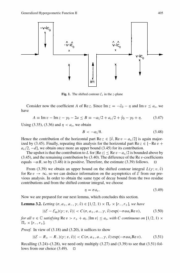
(Hence no indentation is needed for m ≥ −c0 +as/2, for instance.) Likewise, if need bewe indent the contour upwards at Re z = ±Re v, so that it stays at a distance as/2 from±Re v + i(−∞, −c0 + as]. (We will let Im v vary over [−as, as], so this ensures thatthe pole sequences starting at ±v − ic0 stay below the contour.) We have depicted thesituation in Fig. 1 for a choice of parameters where the three indentations are needed,choosing them rectangular for convenience. The poles of Iren (3.11) lie at ±v − ic0 andon the half lines symbolized by the vertical arrows. We have also chosen Im v = −as .

Denoting the shifted contour just defined by Cs , we deduce from the above that wehave

(E − R+ − R−)(γ ; v, v) = χ(γ )[c(γ ; v)c(γ ; v)]−1∫Cs

Iren(γ ; v, v, z)dz. (3.24)

We may and will put the four z-independent G-functions in Iren in front of the integral.This yields a v-independent prefactor

χ(γ )[c(γ ; v)G(v + iγ0)G(−v + iγ0)]−1 (3.25)

that is bounded as (a+, a−, γ ) varies over �-compacts and v varies over [r−, r+]. Thuswe may and shall omit it in estimating E −R+ −R−. By (3.5) and (3.4), the v-dependentprefactor

P(γ ; v) ≡ [c(γ ; v)G(v + iγ0)G(−v + iγ0)]−1 (3.26)

obeys

|P(a+, a−, γ ; v)| < CP (a+, a−, γ, δ, Im v) exp(α(γ0 − γ0 + a)Re v), (3.27)

for all v ∈ C satisfying Re v > δ, with CP continuous on � × (0, ∞) × R. Therefore,we are left with estimating the integral

L(γ ; v, v) =∫Cs

IL(γ ; v, v, z)dz, (3.28)

where

IL(γ ; v, v, z) ≡ G(z + v + iγ0)G(z − v + iγ0)G(z + v + iγ0)G(z − v + iγ0)

G(z + ia)∏3

j=1 G(z + ia + itj ).

(3.29)

To this end we begin by observing that (3.4) entails

|IL|<Ct(a+, a−, γ, Im v, v, Im z) exp(∓α(2aRe z−Im vRe v)), ±Re z>Re v+as/2,

(3.30)

with Ct continuous on � × R × [r−, r+] × R. Therefore the integrals over the tails ofCs are majorized by

C exp(−α(2a ∓ Im v)Re v). (3.31)

Here and from now on, we use the symbol C to denote a positive function of the param-eters a+, a−, γ and η that can be chosen independent of v ∈ [r−, r+], Im v ∈ [−as, as]and Re v ∈ [r+ + al, ∞), and that is continuous for (a+, a−, γ ) in the parameter set atissue.


In connection with this convention, we add three remarks. First, though the param-eter set on which (3.31) holds true is all of � (1.29), it will be necessary to restrict theparameters in various ways later on. Second, we repeat that we are going to fix the shiftparameter η in (3.21) in a case-dependent way. (Of course, the total contour integral isη-independent, but since we can only estimate it piecemeal, the pieces do have depen-dence on η.) Third, at this stage there seems to be no reason to restrict Im v to [−as, as],but the need for this restriction will become apparent shortly.

Next, we combine these estimates with the bound (3.27) on the prefactor to obtainupper bounds

C exp(α(γ0 − γ0 − a ± Im v)Re v) (3.32)

for the tail contributions to E − R+ − R−. Clearly, for these contributions to convergeto 0 as Re v → ∞, it suffices that we have

|Im v| < γ0 − γ0 + a. (3.33)

At this point we should stress that we do not know whether (3.33) is necessary for con-vergence to 0. This restriction is however essential for our analysis to yield the desiredconvergence. (See also our remarks at the end of Sect. 4 in this connection.)

Indeed, for later purposes we need to let Im v vary at least over [−as, as]. Thus wesee that (3.33) can only hold on all of the latter interval when the parameters satisfy

γ0 − γ0 + a − as > 0. (3.34)

Obviously, this condition is not valid for arbitrary parameters. In Sect. 4, we will seethat for a+ = a− it does hold true on a suitable fundamental domain for the W -action.But when a+ equals a−, (3.34) is plainly false for γ = 0. It should be stressed that thesearguments apply irrespective of the choice of shift parameter η. (Recall that (3.30) holdstrue for all Im z ∈ R.)

Therefore, we proceed in two stages. For the remainder of this section, we choosethe parameters in a subset �r of � defined by the restrictions

as ∈ (0, al/8], (3.35)

‖γ ‖ ≤ as/2, (3.36)

where ‖ · ‖ denotes the euclidean norm on R4. This entails |γµ|, |γµ| ≤ as/2 (recall J

is orthogonal), so that we have

γ0 − γ0 + a − as > al/4. (3.37)

Moreover, the requirement (3.36) is clearly W -invariant. Accordingly, we can use theasymptotics results obtained in this section to complete the proof of Theorem 1.1 in thenext one.

Once we have shown W -invariance of E , we can proceed to the second stage, wherewe choose γ in a fundamental domain for which γ0 − γ0 ≥ 0 with equality only forγ = 0. Due to W -invariance, we can then deduce the asymptotic behavior for arbitraryγ , obtaining Theorem 1.2.

After this sketch of our proof strategy, we turn to estimating the contour integralL(γ ; v, v) (3.28). The pertinent result is the following lemma.


Lemma 3.1. Assume the parameters a+, a− and γ are restricted by (3.35) and (3.36),and the variables v and v by (3.9), (3.10) and

Im v ∈ [−as, as]. (3.38)

Then we have

|L(γ ; v, v)| < C exp(−α(γ0 − γ0 + a + η)Re v), (3.39)

with C defined below (3.31).

Proof. We have already seen that the integrals over the right and left tail are boundedabove by (3.31). Since we have |Im v| ≤ as , we obtain an upper bound

C exp(−αalRe v) (3.40)

for both tail integrals.Next, we examine the integral over the right indentation. On this piece of the contour,

the G-function G(z − v + iγ0) in (3.29) is bounded independently of Re v, and so wededuce from (3.4),

|IL| < C exp(α[−4aRe z + (Im z + γ0)(Re v − Re z) + Im v(Re v + Re z)]/2).

(3.41)

Since |Re z−Re v| ≤ as/2 on the indentation, and since Im v ≤ as , this can be majorizedby

|IL| < C exp(−αalRe v). (3.42)

As the length of the indentation is bounded, its contribution is bounded by (3.40). Pro-ceeding analogously for the left indentation, we see that its contribution is once morebounded by (3.40).

Next, we study the contribution of the middle indentation. We need only consider thetwo v-dependent G-functions in (3.29), since the remaining ones stay bounded. Thuswe get from (3.4)

|IL| < C exp(α[(Im z + γ0)Re v + Im vRe z]). (3.43)

Now Im v and Re z stay bounded and we have Im z ≤ −γ0 − a − η on the middleindentation. Hence we obtain

|IL| < C exp(−α(γ0 − γ0 + a + η)Re v), (3.44)

and since the indentation length is bounded, its contribution to L is majorized by

C exp(−α(γ0 − γ0 + a + η)Re v). (3.45)

We proceed with the horizontal piece of the contour where Re z varies from d (3.23)to Re v − as/2, cf. Fig. 1. On the part from d to v, we can proceed just as for the mid-dle indentation, from which we deduce its contribution is bounded by (3.45). On theremainder, however, we must take all G-functions into account. Doing so, we obtainfrom (3.4),

|IL| < C exp(α[(Im z + γ0)Re v + (Im v − Im z − γ0 − 2a)Re z]),

v < Re z < Re v − as/2.(3.46)


Fig. 1. The shifted contour Cs in the z-plane

Consider now the coefficient A of Re z. Since Im z = −c0 − η and Im v ≤ as , wehave

A ≡ Im v − Im z − γ0 − 2a ≤ B ≡ −al/2 + as/2 + γ0 − γ0 + η. (3.47)

Using (3.35), (3.36) and η < as , we obtain

B < −al/8. (3.48)

Hence the contribution of the horizontal part Re z ∈ [v, Re v − as/2] is again major-ized by (3.45). Finally, repeating this analysis for the horizontal part Re z ∈ [−Re v +as/2, −d], we obtain once more an upper bound (3.45) for its contribution.

The upshot is that the contribution to L for |Re z| ≤ Re v−as/2 is bounded above by(3.45), and the remaining contribution by (3.40). The difference of the Re v-coefficientsequals −αB, so by (3.48) it is positive. Therefore, the estimate (3.39) follows.

From (3.39) we obtain an upper bound on the shifted contour integral L(γ ; v, v)

for Re v → ∞, so we can deduce information on the asymptotics of E from our pre-vious analysis. In order to obtain the same type of decay bound from the two residuecontributions and from the shifted contour integral, we choose

η = σas. (3.49)

Now we are prepared for our next lemma, which concludes this section.

Lemma 3.2. Letting (σ, a+, a−, γ, v) ∈ [1/2, 1) × �r × [r−, r+], we have

|(E − Eas)(γ ; v, v)| < C(σ, a+, a−, γ, v) exp(−σαasRe v), (3.50)

for all v ∈ C satisfying Re v > r+ + al, |Im v| ≤ as , with C continuous on [1/2, 1) ×�r × [r−, r+].

Proof. In view of (3.18) and (3.20), it suffices to show

|(E − R+ − R−)(γ ; v, v)| < C(σ, a+, a−, γ, v) exp(−σαasRe v). (3.51)

Recalling (3.24)–(3.28), we need only multiply (3.27) and (3.39) to see that (3.51) fol-lows from our choice (3.49).


4. Proofs of Theorems 1.1 and 1.2

With Lemmas 2.3 and 3.2 at our disposal, it is not difficult to prove the W -invariance ofthe E-function, as will now be detailed.

Proof of Theorem 1.1. We recall that for v > 0 and parameters restricted by (2.21), wehave already obtained information on the Casorati determinant D(v) (2.24), cf. (2.27)and Lemma 2.3. In addition to (2.21), we at first restrict the parameters by requiring(3.35)–(3.36). For notational convenience, we also choose

a− = as. (4.1)

(On account of the parameter symmetry (1.21), this choice is not a restriction.)Now (3.36) is a W -invariant restriction, so that Lemma 3.2 applies to Ej (v), j = 1, 2,

cf. (2.22)–(2.23). In particular, it follows from Lemma 3.2 that Ej (v) remains boundedas Re v → ∞ for v ∈ [r−, r+] and |Im v| ≤ as . Next, we recall from (3.6) that u(γ ; v)

remains bounded as |Re v| → ∞, uniformly for Im v in R-compacts. Therefore, bothfactors on the rhs of (2.27) remain bounded as Re v → ∞, uniformly for |Im v| ≤ a−/2.In view of the reflection symmetry (1.23), this is also the case for Re v → −∞.

It follows that the entire ia−-periodic functionm(v) remains bounded as |Re v| → ∞,uniformly for v ∈ [r−, r+] and |Im v| ≤ a−/2. From Liouville’s theorem we then inferthat m(v) is constant.

We continue to invoke Lemma 3.2 once more, this time to show the constant equals0. First, we note that we may write (cf. (1.15) and (1.24))

u(p; y) = −∏3

µ=0 G(y − ipµ)G(y + ipµ)

G(2y + ia)G(2y − ia). (4.2)

From this we obtain

u(w(p); y) = u(p; y), ∀w ∈ W. (4.3)

Recalling (2.15), we deduce that the u-functions in the asymptotics (3.50) of Ej (v)

satisfy

u(Jγ (j); −v) = u(Jγ ; −v), j = 1, 2. (4.4)

As a consequence, the finite part of the asymptotics of Ej (v) (as Re v → ∞ withv ∈ [r−, r+] and |Im v| ≤ a−) is the same for j = 1 and j = 2. But then we have

limRe v→∞

D(v) = 0, |Im v| ≤ a−/2, (4.5)

and so the constant vanishes, as announced.The upshot is that the function m(v) vanishes identically. Hence the assumption of

Lemma 2.3 is false, i.e., D(v) vanishes identically. This entails that the quotient

Q(a+, a−, γ, w1, w2, v; v) ≡ E(a+, a−, w1(γ ); v, v)/E(a+, a−, w2(γ ); v, v), (4.6)

satisfies

Q(a+, a−, γ, w1, w2, v; v + ia−/2) = Q(a+, a−, γ, w1, w2, v; v − ia−/2), (4.7)

cf. (2.24).


We have now proved ia−-periodicity of Q(v) for v ∈ [r−, r+] and parametersa+, a−, γ restricted by (2.21), (3.35), (3.36) and (4.1). But for Re v, Re v > 0 (say), thefunctions E1 and E2 are real-analytic in a+, a−, γ for a+, a− > 0 and γ ∈ R

4, and forfixed parameters they are meromorphic in v and v (as follows from I). Therefore, (4.7)holds true for parameters a+, a− > 0, γ ∈ R

4, and variables v, v ∈ C. Now E1 and E2are also invariant under a+ ↔ a−, cf. (1.21). Hence the same is true for Q. But then wehave

Q(a+, a−; v + ia+) = Q(a−, a+; v + ia+) = Q(a−, a+; v) = Q(a+, a−; v), (4.8)

so Q(v) has both period ia− and period ia+.Choosing a+, a− > 0 with a+/a− /∈ Q, it follows that Q(v) is constant. By dense-

ness and real-analyticity in a+, a−, we see that Q(v) is constant for all a+, a− > 0. Apriori, the constant could depend on a+, a−, γ, w1, w2 and v, however.

To show that this is not so, we reconsider (4.6), with v and the parameters restrictedso that Lemma 3.2 applies. Then E1(v) and E2(v) have equal asymptotics as v → ∞, sothat Q(v) equals 1. Invoking once again analyticity, we deduce Q(v) = 1 for arbitraryparameters and variables. Hence Theorem 1.1 follows.

Now that we have proved W -invariance of E , we need only determine the Re v → ∞asymptotics of E for γ in a fundamental domain to handle γ ∈ R

4. (As already becameclear from the analysis leading to (3.34), our proof strategy cannot be directly appliedto arbitrary γ .)

Specifically, we choose

γ ∈ diag(−1, 1, 1, −1)DW, (4.9)

with DW defined by (2.19). Hence we have

0 ≤ |γ3| ≤ −γ2 ≤ −γ1 ≤ γ0. (4.10)

This entails

γ0 ≤ γ0/2, (4.11)

so that

γ0 − γ0 + a − as ≥ γ0/2 + (al − as)/2. (4.12)

If we now reconsider the contribution of the tail integrals for this γ -choice (cf. the par-agraph containing (3.34)), we are led to a dichotomy. To be specific, for γ0 > 0 or al > as

we see that it converges exponentially to 0 as Re v → ∞, with a rate that can be chosenuniformly for |Im v| ≤ as . But when we have both γ0 = 0 (which entails γ = 0) andal = as = a, then we only get exponential convergence to 0 for |Im v| ≤ a − ε, ε > 0,with a rate that goes to 0 as ε → 0. On the other hand, the tail contribution does remainbounded as Re v → ∞, uniformly for |Im v| ≤ a, cf. (3.31)–(3.32).

After these introductory observations, we are prepared to complete the proof ofTheorem 1.2.

Proof of Theorem 1.2. Since Eas(a+, a−, γ ; v, v) (1.31) is manifestly W -invariant andE(a+, a−, γ ; v, v) is also W -invariant (as proved in Theorem 1.1), we may and willrestrict γ by (4.9). Moreover, both functions are uniformly bounded on any compactsubset of the set � × {Re v > 0} × (0, ∞), since they are real-analytic in a+, a−, γ, v


and analytic in v on the latter set. Therefore, we need only prove the bounds in thetheorem for v varying over an arbitrary interval [r−, r+] with 0 < r− < r+, and for δ

equal to r+ + al . Hence we can follow the reasoning in Sect. 3.Specifically, recalling the analysis leading to (3.18) and (3.20), we deduce that to

obtain (1.32) , it suffices to show

|(E − R+ − R−)(a+, a−, γ ; v, v)| < C(σ, a+, a−, γ, v) exp(−σαasv), (4.13)

for all v > r+ + al , with C continuous on [1/2, 1) × � × [r−, r+]. Adapting the argu-ments below (3.24), we first obtain (3.31) and (3.32) with Im v = 0. Due to our γ -choice(4.9), we have γ0 − γ0 ≤ 0, so the tail contributions to E − R+ − R− are majorized by

C exp(−αav). (4.14)

On the right indentation we may invoke (3.41) with Im v = 0. Arguing as before, wesee that its contribution to E − R+ − R− is bounded by

C exp(α(γ0 − γ0 − a)v). (4.15)

Repeating the reasoning for the left indentation, we obtain again an upper bound (4.15)for its contribution. Since γ0 − γ0 ≤ 0, the bound (4.15) is majorized by (4.14).

Turning to the middle indentation, we are once more led to (3.45), so its contributionto E − R+ − R− is bounded by

C exp(−αηv). (4.16)

(Recall we need to multiply by (3.27).) More generally, we obtain this bound on the partof the contour where we have −v < Re z < v.

Next, we invoke (3.46) with Im v = 0. The coefficient of Re z equals

c0 + η − γ0 − 2a = γ0 − γ0 + η − a ≤ η − a < 0, (4.17)

since η < as . Choosing η = σas from now on, so that

Im z + γ0 = −γ0 + γ0 − a − σas (4.18)

on this part of the contour, we deduce that its contribution to E − R+ − R− is boundedby

C exp(−σαasv). (4.19)

Likewise, the part Re z ∈ [−v + as/2, −d] leads to (4.19). Putting the pieces together,we obtain (4.13) and hence (1.32).

We proceed with the special case γ = 0, a+ = a− = as = al = a. Thus we havec0 = c0 = a and m = 0 (cf. (3.22)), while (3.27) reduces to

|P(a, a, 0; v)| < CP (a, a, 0, δ, Im v) exp(αaRe v). (4.20)

As we have already pointed out, in this case our estimates on the contribution of thetail integrals to the rhs of (3.24) yield an upper bound

C exp(α(−a + |Im v|)Re v), (4.21)


cf. (3.32). For |Im v| ≤ τa with τ ∈ [0, 1), this is bounded by a multiple of exp((τ −1)αaRe v), but for |Im v| ≤ a we can only deduce boundedness. Proceeding as in theproof of Lemma 3.1, we reach the same conclusion for the right and left indentations.

Since m = 0 in this special case, no middle indentation occurs. For Re z ∈ [−v, v]we obtain as before from (3.4),

|IL| < C exp(−α(a + η)Re v). (4.22)

Combining this with (4.20), we see that the contribution of this line segment to the rhsof (3.24) is majorized by

C exp(−αηRe v). (4.23)

Turning to the bound (3.46), we see it reduces to

|IL| < C exp(α[(−a − η)Re v + (Im v − a + η)Re z]), v < Re z < Re v − a/2.

(4.24)

Taking Im v = a, we infer from (4.20) that the contribution of this line segment cannotbe bounded by (4.23). (Recall C is by definition independent of Im v ∈ [−a, a].) Onthe other hand, fixing η ∈ (0, a), we get for Im v ≤ a:

|∫ Re v−a/2−ia−iη

v−ia−iη

dzIL(γ ; v, v, z)| < C exp(α(−a − η)Re v)

∫ Re v

0dxeαηx

< C exp(−αaRe v). (4.25)

Combined with (4.20), this yields boundedness for |Im v| ≤ a.Fixing τ ∈ [0, 1) and σ ∈ [1/2, 1) and taking Im v ≤ τa, η = σ(1 − τ)a, we have

Im v − a + η ≤ (σ − 1)(1 − τ)a < 0. Then the contribution of the pertinent integral to(3.24) is bounded above by

C(σ, a, τ, v) exp(−αηRe v), η = σ(1 − τ)a, (4.26)

where C is continuous on [1/2, 1) × (0, ∞) × [0, 1) × [r−, r+]. Repeating these argu-ments for the line segment −Re v + a/2 < Re z < −v, we obtain the same conclusion.

The upshot is that the rhs of (3.24) is bounded uniformly for |Im v| ≤ a and v ∈[r−, r+], whereas for |Im v| ≤ τa with τ ∈ [0, 1), this can be improved to (4.26).Recalling our previous results (3.18) and (3.20), we see that we have now proved thedecay assertion (1.34), whereas (1.36) has only been shown to hold for |Im v| ≤ a.

To extend (1.36) to Im v ∈ R, we invoke the A�E

E(v − ia, v) + Va(v)E(v + ia, v) + Vb(v)E(v, v) = 2 cosh(2πv/a)E(v, v), (4.27)

and the bounds (3.7)–(3.8) on Va and Vb. Specifically, taking v → v + ia in (4.27),we obtain (1.36) for Im v ∈ [−2a, −a]. Clearly, we can now proceed in a recursive,strip-by-strip fashion to deduce (1.36) for Im v ∈ (−∞, −a]. Multiplying (4.27) byVa(v)−1, we can take v → v − ia to obtain (1.36) for Im v ∈ [a, 2a], and then recur-sively for Im v ∈ [a, ∞). Thus we have now proved Theorem 1.2 for the special caseγ = 0, a+ = a−.

It remains to prove (1.33) for v ∈ [r−, r+], Re v > r+ + al and γ satisfying (4.9),with a+ = a− in case γ0 = 0. Setting

r ≡ γ0 − γ0 + a − as, (4.28)


we have r > 0 (cf. (4.12)), and the tail contributions to E −R+ −R− are bounded aboveby

C exp(−αrRe v)), (4.29)

cf. (3.32). Using the bound (3.41) for the right indentation and its counterpart for theleft one, we deduce that their contribution is also majorized by (4.29).

Turning to the middle indentation, we conclude as before that its contribution to L

is bounded above by (3.45). Combining this with (3.27), we see that its contribution toE − R+ − R− is majorized by

C exp(−αηRe v). (4.30)

Again, we obtain the same result for the line segments d ≤ |Re z| ≤ v.Next, consider the bound (3.46). In the present case, the coefficient A of Re z satisfies

A ≤ as + γ0 + η − γ0 − a = η − r. (4.31)

Thus we can ensure that it is negative by choosing η in (0, min(as, r)). Doing so, thecontribution of this piece of Cs to E − R+ − R− is again bounded above by (4.30). For−Re v + as/2 < Re z < −v, we reach the same conclusion.

In summary, we have

|(E − R+ − R−)(γ ; v, v)| < C exp(−αηRe v), η ∈ (0, min(as, r)), (4.32)

with r given by (4.28). Recalling (3.18) and (3.20), we deduce

|(E − Eas)(γ ; v, v)| < C exp(−ρRe v), ρ ≡ α min(σas, r). (4.33)

As a consequence, (1.33) follows with Im v ∈ [−as, as]; for γ restricted by (4.9), wecan choose for instance

ρ(a+, a−, γ ) = α min(as/2, γ0 − γ0 + a − as), (4.34)

and this choice can be extended to arbitrary (a+, a−, γ ) ∈ �∗ by requiring that ρ beW -invariant.

Finally, to extend (1.33) to Im v ∈ R, we exploit the eigenvalue A�E for E thatinvolves v-shifts over ±ias . To avoid clumsy formulas, we assume from now on as = a−.(The case as = a+ reduces to obvious notation changes. Alternatively, we can invoke(1.21).) Accordingly, we start from the A�E,

F(v − ia−) + Va(a+, a−, γ ; v)F (v + ia−) + Vb(a+, a−, γ ; v)F (v)

= 2 cosh(αa−v)F (v),(4.35)

obeyed by E(a+, a−, γ ; v, v). Just as in the special case already handled, this can bedone recursively, so we only detail the first step.

Specifically, taking v → v + ia− in the A�E (4.35), we see that we may write

(E−Eas)(v, v) = − exp(iαvv)+u(γ ; −v) exp(−iαvv)−Va(v+ia−)E(v+2ia−, v)

+[exp(αa−v) + exp(−αa−v) − Vb(v + ia−)]E(v + ia−, v). (4.36)

Letting Im v ∈ [−2a−, −a−], we are entitled to use (1.33) for the E-functions on therhs. Doing so, and using also (3.7)–(3.8), we see that the eight terms staying away from0 as Re v → ∞ cancel pairwise. Noting ρ < αa−, the remaining terms manifestly havedecay O(exp(−ρRe v)). Therefore, (1.33) holds for Im v ∈ [−2a−, −a−].


With Theorem 1.2 proved, we can shed more light on the asymptotics of the shiftedcontour integral L(γ ; v, v) (3.28), both for γ that do not satisfy (3.34) and for|Im v| > as . Indeed, from (3.18), (3.20) and Theorem 1.2 we deduce

(E − R+ − R−)(γ ; v, v) = O(exp(−ρRe v)), Re v → ∞, (4.37)

where we have ρ > 0 for arbitrary (fixed) γ ∈ R4 \ {0} and uniformly for Im v in

arbitrary R-compacts. Choosing in particular Im v ∈ [−as, as], we may invoke (3.24),and all of the arguments leading to (3.33) apply as well.

The point is now that (3.4) also yields lower bounds on the prefactors (3.25), (3.26)of the same type as the upper bounds. (That is, (3.25) is bounded away from 0, and wemay also take |P | → |P |−1 in (3.27).) From this we see that for arbitrary a+, a− andγ = 0 we have

L(γ ; v, v) = O(exp([α(γ0 − γ0 − a) − ρ]Re v)), ρ > 0, Re v → ∞, (4.38)

uniformly for |Im v| ≤ as ; provided we enlarge the right and left indentations of Cs (sothat the pole sequences starting at ±v − ic0 stay below Cs), we obtain (4.38) even forIm v in an arbitrary R-compact.

We now explain why this estimate is remarkable. To this end we point out that whenwe use (3.2)–(3.3) to bound IL (3.29) for Re z > Re v + al , it becomes clear that wehave not only

|IL| ∈ exp(−α(2aRe z − Im vRe v))(C−, C+), 0 < C− < C+, Re z > Re v + al,

(4.39)

but also that we are estimating away only one diverging phase (as Re v → ∞), viz., thefactor exp(−iα(Re v)2/2). Since this factor is z-independent, it is quite plausible (thoughit does not rigorously follow) that the modulus of the integral over Re z > Re v + al isbounded below by K exp(α(Im v − 2a)Re v), with K > 0.

Assuming this is indeed the case, we see from (4.38) that whenever we have Im v−a ≥γ0 − γ0, the quotient of the integral over the contour tail Re z > Re v+al and the integralL over the whole contour Cs diverges exponentially as Re v → ∞. This comparisonreveals why our piecemeal reasoning cannot be directly applied to arbitrary Im v andγ . In this connection we should also draw the reader’s attention to the phase factorexp(iα(Re z)2/2) that is estimated away in (3.46). Since it is divergent on the perti-nent interval, it can (and apparently does) supply the cancellations that must occur forIm v − a ≥ γ0 − γ0.

In view of this state of affairs, it may be regarded as a felicitous circumstance that theredoes exist an (Im v)- and γ -window that is not only accessible via piecewise estimates,but large enough to open up the asymptotics of E for arbitrary Im v and γ .

Acknowledgements. We would like to thank the referee for some valuable suggestions.

References

1. Ruijsenaars, S. N. M.: A generalized hypergeometric function satisfying four analytic differenceequations of Askey-Wilson type. Commun. Math. Phys. 206, 639–690 (1999)

2. Ruijsenaars, S. N. M.: Systems of Calogero-Moser type. In: Proceedings of the 1994 Banff summerschool Particles and fields. CRM Ser. in Math. Phys., Semenoff, G., Vinet, L., eds., New York:Springer, 1999, pp. 251–352


3. Askey, R., Wilson, J.: Some basic hypergeometric orthogonal polynomials that generalize Jacobipolynomials. Mem. Am. Math. Soc. 319, (1985)

4. Gasper, G., Rahman, M.: Basic hypergeometric series. In: Encyclopedia of Mathematics and itsApplications. 35, Cambridge: Cambridge Univ. Press 1990

5. Ruijsenaars, S. N. M.: Special functions defined by analytic difference equations. In: Proceedingsof the Tempe NATO Advanced Study Institute “Special Functions 2000”, NATO Science SeriesVol. 30, Bustoz, J., Ismail, M., Suslov, S., eds., Dordrecht: Kluwer, 2001, pp. 281–333

6. Ruijsenaars, S. N. M.: Sine-Gordon solitons vs. relativistic Calogero-Moser particles. In: Proceed-ings of the Kiev NATO Advanced Study Institute “Integrable structures of exactly solvable two-dimen-sional models of quantum field theory”, NATO Science Series Vol. 35, Pakuliak, S., von Gehlen, G.,eds., Dordrecht: Kluwer, 2001, pp. 273–292

7. Ruijsenaars, S. N. M.: A generalized hypergeometric function III. Associated Hilbert space trans-form. To appear in Commun. Math. Phys. - DOI 10.1007/s00220-003-0970-x

8. Koornwinder, T. H.: Askey-Wilson polynomials for root systems of type BC. Contemp. Math. 138,189–204 (1992)

9. van Diejen, J. F.: Self-dual Koornwinder-Macdonald polynomials. Invent. Math. 126, 319–339(1996)

10. Grunbaum, F. A., Haine, L.: Some functions that generalize the Askey-Wilson polynomials. Com-mun. Math. Phys. 184, 173–202 (1997)

11. Ismail, M. E. H., Rahman, M.: The associated Askey-Wilson polynomials. Trans. Am. Math. Soc.328, 201–237 (1991)

12. Suslov, S. K.: Some orthogonal very-well-poised 8φ7-functions. J. Phys. A: Math. Gen. 30, 5877–5885 (1997)

13. Suslov, S. K.: Some orthogonal very-well-poised 8φ7-functions that generalize Askey-Wilson poly-nomials. The Ramanujan Journal 5, 183–218 (2001)

14. Koelink, E., Stokman, J. V.: The Askey-Wilson function transform. Int. Math. Res. Notes No. 22,1203–1227 (2001)

15. Stokman, J. V.: Askey-Wilson functions and quantum groups. Preprint, math.QA/030133016. Ruijsenaars, S. N. M.: Relativistic Lame functions revisited. J. Phys.A: Math. Gen. 34, 10595–10612

(2001)

Communicated by L. Takhtajan

Documents

A Generalized Hypergeometric Function II. Asymptotics and ...siru/papers/p61.pdf · Generalized Hypergeometric Function II 391 Finally, the contour C is given by a horizontal line