Embed Size (px)
Citation preview
Hypergeometric Series Representations of FeynmanIntegrals by GKZ Hypergeometric Systems
Rene Pascal Klausen∗
October 22, 2019
Abstract
We show that almost all Feynman integrals as well as their coefficients in aLaurent series in dimensional regularization can be written in terms of Horn hy-pergeometric functions. By applying the results of Gelfand-Kapranov-Zelevinsky(GKZ) we derive a formula for a class of hypergeometric series representations ofFeynman integrals, which can be obtained by triangulations of the Newton poly-tope ∆G corresponding to the Lee-Pomeransky polynomial G. Those series can beof higher dimension, but converge fast for convenient kinematics, which also allowsnumerical applications. Further, we discuss possible difficulties which can arise in apractical usage of this approach and give strategies to solve them.
Introduction
In the early days of calculating Feynman amplitudes, it was proposed by Regge to considerFeynman integrals as a kind of generalized hypergeometric functions [60], where the sin-gularities of those hypergeometric functions coincide with the Landau singularities. Lateron Kashiwara and Kawai [43] showed that Feynman integrals satisfy indeed holonomicdifferential equations, where the singularities of those holonomic differential equations aredetermined by the Landau singularities.
Apart from characterizing the Feynman integral by “hypergeometric” partial differ-ential equation systems, many applications determine the Feynman integral as a general-ized hypergeometric series. Usually, the often used Mellin-Barnes approach [68] results inPochhammer series pFq, Appell functions, Lauricella functions and related functions byapplying the residue theorem [8]. Furthermore, for arbitrary one-loop Feynman integralsit is known that they can always be represented by a small set of hypergeometric series[24]. Thirdly, the Feynman integral may be expressed by “hypergeometric” integrals likethe generalized Meijer G- or Fox H-functions [15, 39, 40].
Thus there arise three different notions of the term “hypergeometric” in the Feyn-man integral calculus, where every notion generalizes different characterizations of theclassical hypergeometric Gauß function 2F1(a, b, c;x). In the late 1980s Gelfand, Kapra-nov, Zelevinsky (GKZ) and collaborators [26–31] were starting to develop a comprehensivemethod to generalize the notion of “hypergeometric” functions in a consistent way. Those
∗Department of Physics at Humboldt University of Berlin and Max-Planck-Institute for GravitationalPhysics (Albert-Einstein-Institute) in Potsdam-Golm ([email protected])
1
arX
iv:1
910.
0865
1v1
[he
p-th
] 1
8 O
ct 2
019
functions are called A-hypergeometric functions and are defined by a special holonomicsystem of partial differential equations.
As Gelfand, Kapranov and Zelevinsky illustrated with Euler integrals, the GKZ ap-proach not only generalizes the concept of hypergeometric functions but can also be usedfor analyzing and solving integrals [30].
For physicists the GKZ perspective is not entirely new. Already in the 1990s, stringtheorists applied the GKZ approach in order to calculate period integrals and workedout the mirror symmetry [37, 38]. Recently, the GKZ approach was also used to obtaindifferential equations for the Feynman integral from the maximal cut [74]. Still, theapproach of Gelfand, Kapranov and Zelevinsky is no common practice among physicists.
In 2016 Nasrollahpoursamami showed that the Feynman integral satisfies a differentialequation system which is isomorphic to a GKZ system [52]. Very recently1, this fact wasalso shown directly in [20] based on the Lee-Pomeransky representation of the Feynmanintegral.
Beyond the above statement which characterizes generic Feynman integrals as A-hypergeometric functions, we show that generic Feynman integrals as well as every co-efficient in the ε expansion in dimensional regularization belong to the class of Hornhypergeometric functions. Furthermore, we give an explicit formula for a multivariateseries representation of a generic Feynman integral for unimodular triangulations. Thisallows, to evaluate the Feynman integral efficiently for convenient kinematic regions.
Therefore, from the perspective of GKZ it turns out that Horn hypergeometric func-tions and Feynman integrals share many properties, e.g. Horn hypergeometric functionssatisfy special relations similar to the IBP-relations of the Feynman integral [47]. In thisarticle, we work out the connection between Feynman integrals and Horn hypergeomet-ric functions from the GKZ perspective and we give a strategy, as to how to use thisknowledge in the evaluation of Feynman integrals.
The connections between Feynman integrals and hypergeometric functions was inves-tigated over decades and a comprehensive summary of these investigations can be foundin [41]. Horn hypergeometric functions also appear often in the Mellin-Barnes approachand have been studied intensively by other authors, e.g [16, 61].
The paper is structured as follows. After recalling the parametric representations ofthe Feynman integral, which are crucial for this approach, we mention some properties ofthe Feynman integral, which can be obtained from their algebraic geometry description.This first section will also include a short mathematical interlude about convex polytopes,which are necessary in the description of the properties of Feynman integrals, as well asin the later GKZ approach. Secondly, we briefly introduce the GKZ hypergeometricsystem, which is a system of partial differential equations and recall a series solution ofthose systems. This leads us to the last section, in which we merge these two aspects inorder to derive an analytical series representation of the Feynman integral. To completethis section we also discuss some features as well as possible difficulties which can arisein the evaluation of Feynman integrals with GKZ systems. We conclude this article bycalculating the full massive sunset Feynman diagram as a non-trivial example in order toillustrate this procedure and to give a glimpse of its further scope of application.
Acknowledgements: This research is supported by the International Max Planck Re-search School for Mathematical and Physical Aspects of Gravitation, Cosmology and
1The present paper was developed independently from [20], which the author noticed just shortlybefore publication.
2
Quantum Field Theory. I would like to express my special thanks to Christian Bognerfor his great encouragement, his supervision and his assistance in difficult circumstances.Further, I would like to thank Dirk Kreimer for his support, organizational skills and forincluding me in his group. I am also grateful to Josua Faller and Tatiana Stahlhut fortheir proofreading and all the members of Dirk Kreimer’s group for helpful discussions.
1 Feynman Integrals
In this section we shortly recall the parametric representations of Feynman integrals,which are based on graph polynomials [7]. Those parametric representations containnormally two graph polynomials, known as the Symanzik polynomials. Recently, Leeand Pomeransky [48] introduced a parametric representation, which depends only on onegraph polynomial, which simplifies the application of the Gelfand-Kapranov-Zelevinskyapproach. In this representation the Feynman integral can be formally described as amultivariate Euler-Mellin integral.
In the second part of this section, we rely on some general properties of Euler-Mellinintegrals in order to recall some basic properties of the Feynman integral from the per-spective of the Lee-Pomeransky representation. To keep this discussion short, we refer tostandard literature [68, 70, 77] for further properties of the Feynman integral.
Since the formulation of this properties of Feynman integrals, as well as the laterintroduced GKZ approach, include convex polytopes, we give a short mathematical inter-lude about convex polytopes between these two parts. A proceeding and more detaileddescription of polytopes can be found in the appendix.
1.1 Parametric Representations of Feynman Integrals
The Feynman integral in momentum space is an (Ld)-dimensional loop integral overpropagators. Since propagators are at most quadratic in the loop momenta, one canrewrite the Feynman integral as an n-dimensional integral over Schwinger parametersx1, . . . , xn ∈ R≥0 [57]. With this rephrasing one can make the Feynman integral alsomeaningful for d ∈ C, as required in the procedure of dimensional regularization [73].
In the parametric version of Feynman integrals, two polynomials in the Schwingerparameters arise, which are known as first and second Symanzik polynomial [7]
U =∑T∈T1
∏ei /∈T
xi (1.1)
F = −∑F∈T2
sF∏ei /∈F
xi + U∑ei∈E
xim2i . (1.2)
Here, Ti is the set of spanning forests of the Feynman graph Γ consisting of i components,E denotes the set of all edges of Γ and sF is the squared momentum flowing from theone component of the 2-forest F to the other component. For Euclidean kinematicsthe coefficients of all monomials in the second Symanzik polynomial will be positive.In the following we restrict the discussion to Euclidean kinematics in order to avoidzeros of the Symanzik polynomials in the positive orthant x ∈ Rn
>0. Since almost everyFeynman integral with Minkowskian kinematics has a non-vanishing overlap with theEuclidean region, one can extend the Euclidean result to the Minkowskian result by
3
analytic continuation. In this procedure additional divergences can appear and thus theanalytic continuation can be far from trivial [57].
As the starting point of this discussion we define the Feynman integral in the Feynmanparametric representation.
Definition 1.1 [Feynman integral]: For a given Feynman graph Γ with n edges, Lloops2 and the Symanzik polynomials U and F , the Feynman integral is given as ann-dimensional integral
IΓ(ν, d, p,m) :=Γ(ω)
Γ(ν)
∫Rn+
dx xν−1δ
(1−
n∑i=1
xi
)Uω− d
2
F ω(1.3)
where ω :=∑n
i=1 νi− Ld2
is the superficial degree of divergence and δ(x) denotes the Diracδ function. The ν ∈ Cn with Re νi > 0 are the propagator powers. Note that for simplicitywe use a multi-index notation throughout the whole paper, which implies the followingshorthand notations
dx := dx1 · · · dxn
xν−1 := xν1−11 · · ·xνn−1
n (1.4)
Γ(ν) := Γ(ν1) · · ·Γ(νn) .
Clearly, those integrals converge not for every values of ν ∈ Cn and d ∈ C andalso not for every choice of the polynomials U and F . It can be shown, that besidesof the class of massless tadpole graphs, these integrals define meromorphic functions inν and d. Therefore, we will consider the Feynman integral always as the meromorphiccontinuation of the integral (1.3) to the whole complex plane. The convergence as well asthe meromorphic expansion will be discussed in more detail in section 1.3.
Remark: One is often interested in νi ∈ N. However, in the following it will be conve-nient to consider a slightly more general notion of Feynman integrals where the propagatorpowers νi are not restricted to integer values only. Just the restriction Re νi > 0 is nec-essary to guaranty the parametric rewriting and convergence. These conditions are oftenassumed in the literature e.g. in [6, 69].
The parametric representation in equation (1.3) is not the only representation in termsof Schwinger parameters. For the following approach another parametric representationinvented by Lee and Pomeransky [48] is more convenient.
Theorem 1.1 [Lee-Pomeransky representation [48]]: The Feynman integral from equa-tion (1.3) can also be written as
IΓ(ν, d, p,m) =Γ(d2
)Γ(d2− ω
)Γ(ν)
∫Rn+
dx xν−1G−d2 , (1.5)
where the integral depends only on the sum of Symanzik polynomials G = U + F , whichwe call the Lee-Pomeransky polynomial G. The equality of representations is in the senseof meromorphic extension.
2In contrast to the nomenclature in graph theory, in the context of Feynman integrals a “loop” meansa closed path. Thus, L is the first Betti number of Γ.
4
Proof. (A proof can be found also in [6]) Since U is homogeneous of degree L and F ishomogeneous of degree L+1, the integral in (1.5) as a function of d converges in the strip
Λ ={d ∈ C
∣∣∣2 Re∑i νi
L+1< Re d <
2 Re∑i νi
L
}. As we consider Re νi > 0 it is Λ 6= ∅. For an
equality in the sense of meromorphic extension it is sufficient to show that there is anon-vanishing interval where the equality of representations holds.
Inserting 1 =∫∞
0ds δ(s −∑i xi) in (1.5), changing the integration order and substi-
tuting xi → sxi one obtains
IΓ(ν, d, p,m) =Γ(d2
)Γ(d2− ω
)Γ(ν)
∫ ∞0
ds
∫Rn+
dx δ(s− s∑i
xi)xν−1s
∑i νi(sLU + sL+1F )−
d2 .
(1.6)
Since the integral∫∞
0ds s
∑i νi−L
d2−1(U + sF )−
d2 can be calculated explicitly as a beta
function in the region Λ (and for U, F > 0) one attains the representation (1.3).
Thus, the whole structure of a Feynman integral can be expressed in only one singlepolynomial G ∈ C[x1, . . . , xn] . As it is possible for every polynomial, one can write theLee-Pomeransky polynomial G as
Gz(x) =∑aj∈A
zjxaj =
N∑j=1
zjxa1j
1 . . . xanjn (1.7)
where A is a finite set consisting of N pairwise distinct column vectors aj ∈ Zn≥0 and thecoefficients of this polynomial are complex numbers z ∈ (C \ {0})N , which contain thekinematics and masses. This representation is unique, up to the possibility of differentmonomial orderings. Without loss of generality we can fix an arbitrary monomial orderingand we denote the set of column vectors A in a matrix structure. As we will observe later,the exponential vectors of the Lee-Pomeransky polynomial Gz satisfy an affine structure.Thus, it will be convenient to define
A :=
(1A
)=
(1 1 . . . 1a1 a2 . . . aN
)∈ Z(n+1)×N
≥0 . (1.8)
Further, for an index set σ ⊂ {1, . . . , N} the notation Aσ denotes the restriction of Aaccording to columns indexed by σ.
In addition, we define coordinates ν := (ν0, ν) ∈ Cn+1, where the first entry of νcontains the physical dimension ν0 := d
2. From a mathematical point of view, the physical
dimension d and the propagator powers νi have a similar role in parametric Feynmanintegrals. This is the reason why instead of using dimensional regularization one can alsoregularize the integral by considering the propagator powers as complex numbers as donein analytic regularization [69].
In fact, this definition of Gz(x) includes a generalization of the original Feynmanintegral, since also the first Symanzik polynomial gets coefficients zi. Thus, we define:
Definition 1.2 [Generic Feynman Integrals]: Let Gz(x) a Lee-Pomeransky polynomialwith generic coefficients z ∈ CN satisfying Re zj > 0. The generic Feynman integral isthe meromorphic continuation of the integral
JA(ν, z) := Γ(ν0)
∫Rn+
dx xν−1Gz(x)−ν0 . (1.9)
defined on ν = (ν0, ν) ∈ Cn+1.
5
Remark: In this definition the complete graph structure, which is necessary to evaluatethe Feynman integral, is given by the matrix A. The variables z ∈ CN contain thephysical information about kinematics and masses and the ν ∈ Cn+1 are the regularizationparameters.
In contrast to equation (1.5) the coefficients in Gz which come from the first Symanzikpolynomial are treated as generic, instead of equal to 1. We will discuss later how one canremove these auxiliary variables afterwards to obtain the “ordinary” Feynman integral.To avoid unnecessary prefactors in the following, we omit also the factor Γ(ν0 − ω)Γ(ν)in this definition
With this definitions one can derive another representation of the Feynman integralas a multi-dimensional Mellin-Barnes integral.
Theorem 1.2 [Representation as Fox H-function]: Let σ ⊂ {1, . . . , N} be an indexsubset with cardinality n+1, such that the matrix A restricted to columns of σ is invertible,detAσ 6= 0. Then the Feynman integral can be written as the multi-dimensional Mellin-Barnes integral
JA(ν, z) =z−A
−1σ ν
σ
| detAσ|
∫γ
dt
(2πi)rΓ(t)Γ(A−1
σ ν −A−1σ Aσt)z−tσ zA
−1σ Aσt
σ (1.10)
wherever this integral converges. The set σ := {1, . . . N}\σ denotes the complement of σ,containing r := N − n− 1 elements. Restrictions of vectors and matrices to those indexsets are similarly defined as zσ := (zi)i∈σ, zσ := (zi)i∈σ, Aσ := (ai)i∈σ. Every componentof the integration contour γ ∈ Cr goes from −i∞ to i∞ such that the poles of the integrandare separated.
Corollary 1.3: Let N = n + 1 or in other words let A be quadratic. If there is aregion D ⊆ Cn+1 such that the Feynman integral JA(ν, z) converges absolutely for ν ∈ D,the matrix A is invertible and the Feynman integral is only a simple combination of Γ-functions:
JA(ν, z) =Γ(A−1ν)
| detA| z−A−1ν . (1.11)
Proof. Starting from equation (1.9) by the Schwinger trick one gets
JA(ν, z) =
∫Rn+1
+
dx0 xν0−10 dx xν−1e−x0G , (1.12)
where ν0 = d2. Writing x = (x0, x), ν = (ν0, ν) and using the Cahen-Mellin integral
representation of exponential function one obtains
JA(ν, z) =
∫Rn+1
+
dxxν−1
∫δ+iRn+1
du
(2πi)n+1Γ(u)z−uσ x−Aσu
∫δ+iRr
dt
(2πi)rΓ(t)z−tσ x
−Aσt
(1.13)
with u ∈ Cn+1, t ∈ Cr, some arbitrary positive numbers δi > 0 and where we split thepolynomial G into a σ and a σ part. By a substitution u→ A−1
σ u′ it is
JA(ν, z) = | detA−1σ |∫δ+iRr
dt
(2πi)rΓ(t)z−tσ∫
Rn+1+
dx
∫Aσδ+iAσRn+1
du′
(2πi)n+1Γ(A−1
σ u′)z−A−1σ u′
σ xν−u′−Aσt−1 .
(1.14)
6
Since the matrix Aσ contains only positive values, the integration region remains thesame Aσδ + iAσRn+1 ' δ′ + iRn+1 with some other positive numbers δ′ ∈ Rn+1
>0 , whichadditionally have to satisfy A−1
σ δ′ > 0. By Mellin’s inversion theorem [1] only the t-integration remains and one obtains equation (1.10).
Thereby, the integration contour has to be chosen, such that the poles are separatedfrom each other in order to satisfy A−1
σ δ′ > 0. More specific this means that the contourγ has the form c+ iRn+1 where c ∈ Rn+1
>0 satisfies A−1σ ν −A−1
σ Aσc > 0. Clearly, in orderfor those c to exist, the possible values of parameters ν are restricted.
The proof of the corollary is a special case, where one does not have to introduce theintegrals over t. The existence of the inverse A−1 is ensured by theorem 1.4.
Remark: A more general version of this theorem can be found in [3, thm. 5.6] with anindependent proof. In [72] a similar technique is used to obtain Mellin-Barnes represen-tations from Feynman integrals.
The convergence of those Mellin-Barnes representation is discussed in [34] and generalaspects of multivariate Mellin-Barnes integrals can be found in [58].
The corollary can alternatively be proven by splitting the term G−ν0 by the multino-mial theorem in a multidimensional power series and solve the Mellin transform of thispower series by a generalized version of Ramanujan’s master theorem [32].
The type of the integral which appears in equation (1.10) is also known as multivariateFox H-function [34] and the connection between Feynman integrals and Fox H-functionwas studied before [15, 39, 40].
Since the number of monomials in the Symanzik polynomials increases fast for morecomplex Feynman graphs, the Mellin-Barnes representation of theorem 1.2 does not pro-vide an efficient way to calculate those integrals. One exception are the massless 2-pointfunctions consisting in n lines and having the loop number L = n − 1. These so-called“banana graphs” or “sunset-like” graphs, have only n + 1 monomials in G and satisfytherefore the condition in the corollary.
In order to illustrate the theorem 1.2 about Mellin-Barnes representations, we finishthis section with a simple example.
p
m2 = 0
m1 6= 0
p
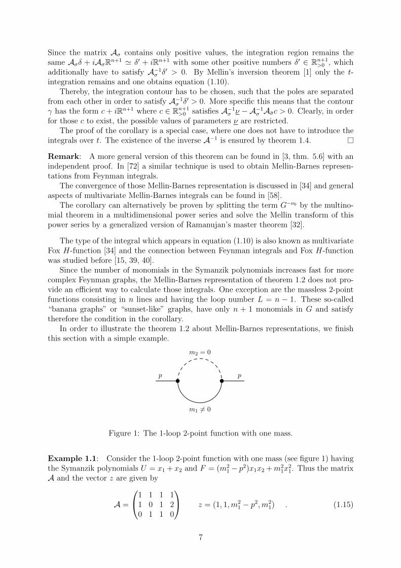
Figure 1: The 1-loop 2-point function with one mass.
Example 1.1: Consider the 1-loop 2-point function with one mass (see figure 1) havingthe Symanzik polynomials U = x1 + x2 and F = (m2
1− p2)x1x2 +m21x
21. Thus the matrix
A and the vector z are given by
A =
1 1 1 11 0 1 20 1 1 0
z = (1, 1,m21 − p2,m2
1) . (1.15)
7
Choosing σ = {1, 2, 3}, the corresponding Feynman integral in the Mellin-Barnes repre-sentation of theorem 1.2 is given by
JA(ν, z) = z−ν0+ν21 z−ν0+ν1
2 zν0−ν1−ν23
∫ δ+i∞
δ−i∞
dt
2πiΓ(t)Γ(ν0 − ν1 + t)
Γ(ν0 − ν2 − t)Γ(−ν0 + ν1 + ν2 − t)(z2z4
z1z3
)−t. (1.16)
For the correct contour prescription the poles have to be separated such that there existvalues δ satisfying max{0,−ν0 +ν1} < δ < min{ν0−ν2,−ν0 +ν1 +ν2}. In the formulationto be introduced in the following section 1.3, this is equivalent to claim a full dimensionalNewton polytope of G. In this case, by Cauchy’s theorem the integral evaluates simplyto a Gaussian hypergeometric function
JA(ν, z) =Γ(2ν0 − ν1 − ν2)Γ(ν2)Γ(ν0 − ν2)Γ(−ν0 + ν1 + ν2)
Γ(ν0)
z−ν0+ν21 z−ν0+ν1
2 zν0−ν1−ν23 2F1
(ν0 − ν2,−ν0 + ν1 + ν2
ν0
∣∣∣∣ 1− z2z4
z1z3
). (1.17)
After restoring the original prefactors and coefficients z1 = z2 = 1, z3 = p2−m21, z4 = m2
1
and ν0 = d2
it agrees with the expected result
IΓ(ν1, ν2, d,m21, p
2) =Γ(d2− ν2
)Γ(−d
2+ ν1 + ν2
)Γ(ν1)Γ
(d2
)(p2 −m2
1)d2−ν1−ν2
2F1
(d2− ν2,−d
2+ ν1 + ν2
d2
∣∣∣∣∣ 1− m21
p2 −m21
).
(1.18)
1.2 Mathematical Interlude: Convex Polytopes
In the following, it will be fruitful to describe properties and solutions of Feynman integralsfrom a perspective of convex polytopes. In order to clarify some terminology, we give ashort review of the basic concepts of convex polytopes. Readers which are familiar withconvex polytopes can skip this interlude. More details about polytopes, customized tothe hypergeometric approach, can be found in the appendix. For further treatments werefer to [11, 13, 21, 35].
A convex polytope P is defined as the convex hull of a finite set of points A ={a1, . . . , aN}
P := Conv(A) :=
{N∑j=1
kjaj
∣∣∣∣∣ k ∈ RN≥0,
N∑j=1
kj = 1
}(1.19)
where ai ∈ Rn. Additionally, if the points ai ∈ Zn form an integer lattice, P is called aconvex lattice polytope. Since in this discussion all polytopes will be convex polytopes,we will call them simply “polytopes” in the following.
As a fundamental result of polytope theory, every polytope can also be written as abounded intersection of half-spaces
P := P (M, b) := {µ ∈ Rn|mTj · µ ≤ bj, 1 ≤ j ≤ k} (1.20)
8
where b ∈ Rk and M ∈ Rk×n are real, mTj denotes the rows of the matrix M and · is the
standard scalar product.The Newton polytope ∆f corresponding to a multivariate polynomial f =
∑α cαx
α ∈C[x1, . . . , xn] is defined as the convex hull of its exponent vectors ∆f := Conv({α|cα 6= 0}).
A subset of P having the form F := {µ ∈ P |c µ = β}, with c ∈ Rk×n and where everypoint of the polytope µ ∈ P satisfies the inequality c µ ≤ β, is called a face of P . Facesof dimension zero are called vertices and faces of dimension n− 1 are called facets. Thus,if equation (1.20) consist in a minimal set of inequalities, the facets of P are given bymTj µ = bj. The polytope without its faces is called the relative interior relintP of the
polytope P .The dimension of a polytope P = Conv(A) is defined as the dimension of its affine
hull, and thus one can easily see
dim(Conv(A)) = rank
(1A
)− 1 . (1.21)
As before in equation (1.8), we will denote the matrix A with an additional row (1, . . . , 1)
as A =
(1A
). If a polytope P ⊂ Rn has the dimension n it is called to be full dimensional
and degenerated otherwise.For full dimensional polytopes it is meaningful to introduce a volume of polytopes. As
the volume vol0(P ) ∈ N of a lattice polytope we understand a volume, which is normalizedsuch that the standard simplex has volume 1. Therefore, this volume is connected to thestandard Euclidean volume vol(P ) by a faculty of the dimension vol0(P ) = n! vol(P ).For a full dimensional simplex P4 = Conv(A) the volume is given by the determinantvol0(P4) = | detA|. Thus, one way of calculating the volume of a polytope is by dividingthe polytope in simplices.
A subdivision of a polytope P into simplices, where the union of all simplices is thefull polytope and the intersection of two distinct simplices is a proper face of the polytope(including the empty set), is called a triangulation.
A triangulation T (ω) = {σ1, . . . , σr} of a polytope P = Conv(A) is called regular, ifthere exists an height vector ω ∈ RN , such that for every simplex σi of this triangulationthere exists another vector ri ∈ Rn+1 satisfying
ri · aj = ωj for j ∈ σiri · aj < ωj for j /∈ σi ,
where · denotes the scalar product.It can be shown, that every convex polytope admits always a regular triangulation [21].
If all σ ∈ T (ω) belongs to simplices with volume 1 (i.e. | detAσ| = 1) the triangulation iscalled unimodular.
In order to reduce later more complicated Feynman integrals to simpler one, we intro-duce subtriangulations.
Definition 1.3 [Subtriangulation]: Let P ⊂ Rn be a polytope and T be a triangulationof P . A simplicial complex T ′ is a subtriangulation of T (symbolically T ′ ⊆ T ) if
a) T ′ is a subcomplex of T (i.e. T ′ is a subset of T , and T ′ is a polyhedral complex) and
b) the union of all simplices in T ′ equals a (convex) polytope P ′ ⊆ P .
9
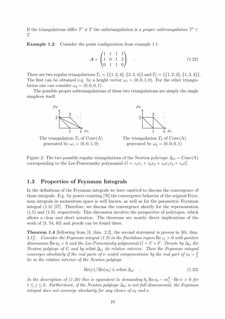
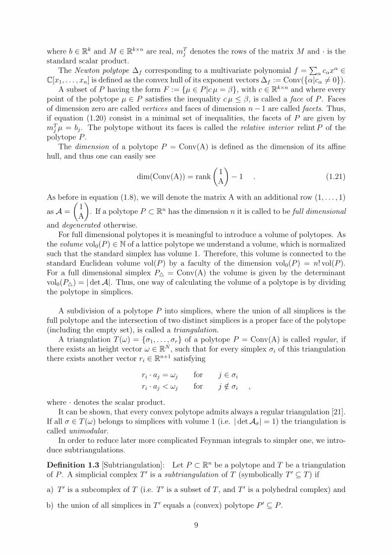
If the triangulations differ T ′ 6= T the subtriangulation is a proper subtriangulation T ′ ⊂T .
Example 1.2: Consider the point configuration from example 1.1
A =
1 1 1 11 0 1 20 1 1 0
. (1.22)
There are two regular triangulations T1 = {{1, 2, 4}, {2, 3, 4}} and T2 = {{1, 2, 3}, {1, 3, 4}}.The first can be obtained e.g. by a height vector ω1 = (0, 0, 1, 0). For the other triangu-lation one can consider ω2 = (0, 0, 0, 1).
The possible proper subtriangulations of these two triangulations are simply the singlesimplices itself.
µ1
µ2
1
23
4 µ1
µ2
1
23
4
The triangulation T1 of Conv(A) The triangulation T2 of Conv(A)generated by ω1 = (0, 0, 1, 0) generated by ω2 = (0, 0, 0, 1)
Figure 2: The two possible regular triangulations of the Newton polytope ∆G = Conv(A)corresponding to the Lee-Pomeransky polynomial G = z1x1 + z2x2 + z3x1x2 + z4x
21.
1.3 Properties of Feynman Integrals
In the definitions of the Feynman integrals we have omitted to discuss the convergence ofthose integrals. E.g. by power counting [76] the convergence behavior of the original Feyn-man integrals in momentum space is well known, as well as for the parametric Feynmanintegral (1.3) [57]. Therefore, we discuss the convergence shortly for the representation(1.5) and (1.9), respectively. This discussion involves the perspective of polytopes, whichallows a clear and short notation. The theorems are mostly direct implications of thework of [3, 54, 65] and proofs can be found there.
Theorem 1.4 [following from [3, thm. 2.2], the second statement is proven in [65, thm.3.1]]: Consider the Feynman integral (1.9) in the Euclidean region Re zj > 0 with positivedimensions Re ν0 > 0 and the Lee-Pomeransky polynomial G = U +F . Denote by ∆G theNewton polytope of G and by relint ∆G its relative interior. Then the Feynman integralconverges absolutely if the real parts of ν scaled componentwise by the real part of ν0 = d
2
lie in the relative interior of the Newton polytope
Re(ν)/Re(ν0) ∈ relint ∆G . (1.23)
In the description of (1.20) this is equivalent to demanding bj Re ν0 −mTj · Re ν > 0 for
1 ≤ j ≤ k. Furthermore, if the Newton polytope ∆G is not full-dimensional, the Feynmanintegral does not converge absolutely for any choice of ν0 and ν.
10
The second statement means, that Feynman integrals which do not have a full-dimensional Newton polytope ∆G are neither dimensionally nor analytically regulariz-able. This result is not surprising, since if the Newton polytope is not full dimensional,the polynomial G has a special homogeneous property. A polynomial G is homogeneousin such that way, that there exists numbers c0, . . . , cn ∈ Z not all zero, such that
Gz(sc1x1, . . . , s
cnxn) = sc0Gz(x1, . . . , xn) (1.24)
holds. If G corresponds to a massless tadpole graph, G is homogeneous in this sense, sincemassless tadpole graphs have F = 0 and the first Symanzik polynomial is homogeneousof degree L. Thus, there will be no values for ν = (ν0, ν) ∈ Cn+1 that those integrals con-verge. However one usually sets those tadpole graphs to zero by including a countertermin the renormalization procedure, which removes all tadpole graphs [70] (see also [6, sec.3.1]).
Since the Feynman integral in (1.9) is only equivalent to the original Feynman integralin the meromorphic extension, the convergence region of (1.9) has no deeper physicalmeaning. Using the following theorem one can deduce the meromorphic continuation of(1.9) to the whole complex plane, which determines the physical relevant poles of theFeynman integral.
Theorem 1.5 [Meromorphic continuation of Feynman integrals [3, thm. 2.4, rem. 2.6]]:Consider a Feynman integral JA in the Euclidean region Re zj > 0 with a full-dimensionalNewton polytope ∆G = {µ ∈ Rn|mT
j · µ ≤ bj, 1 ≤ j ≤ k}. Then one can rewrite theFeynman integral as
JA(ν, z) = ΦA(ν, z)N∏j=1
Γ(bj Re ν0 −mTj · Re ν) (1.25)
where ΦA(ν, z) is an entire function with respect to ν ∈ Cn+1.
Example 1.3: Consider the example from above which correspond to figure 1. For therelative interior of the Newton polytope one obtains from the facet representation, theregion of convergence (with Re ν0 > 0)
Re(ν0 − ν2) > 0 Re(−ν0 + ν1 + ν2) > 0
Re(ν2) > 0 Re(2ν0 − ν1 − ν2) > 0
which enables us to separate the poles of the Feynman integral in the Γ functions
IA(ν, z) = ΦA(ν, z)Γ(−ν0 + ν1 + ν2)Γ(ν0 − ν2)
Γ(ν1)
with an entire function ΦA(ν, z).
This result is remarkable in many different ways. Firstly, it guarantees that the Feyn-man integral can be meromorphically continued to the whole complex plane, which con-firms dimensional and analytical regularization. Secondly, equation (1.25) gives an easymethod to calculate the (possible) poles of the Feynman integral. And thirdly, in the εexpansion one can focus only on a Taylor expansion of ΦA instead of a Laurent expan-sion of JA. Thus, one can determine the coefficients by differentiating, which makes theprocedure much easier.
11
These theorems do not rely on any special properties of the Symanzik polynomials. Infact, Feynman integrals are just a subset of Euler-Mellin integrals. The following lemma isa simple implication from the properties of Symanzik polynomials to be at most quadratic,and to be homogeneous of degree L and L+ 1, respectively.
Lemma 1.6: Let A =
(1A
)be a point configuration coming from a Feynman graph.
a) The entries of the matrix A are restricted to A ∈ {0; 1; 2}(n+1)×N . Every column ofA contains at most one entry equals 2. For massless Feynman integrals the points areeven in A ∈ {0; 1}(n+1)×N .
b) All points in A are arranged on two parallel hyperplanes in Rn. The hyperplanes havethe normal vector (1, 1, . . . , 1) and a distance of 1 between them. This means that theNewton polytopes ∆G arising in Feynman integrals are compressed in one direction.
c) The Newton polytope ∆G, corresponding to a Feynman graph, has no interior points.
Thus, we have reformulated the Feynman integral as an Euler-Mellin integral, whichdefines a meromorphic function in ν ∈ Cn+1. To consider the Euclidean region we haverestricted3 the discussion to the right half space z ∈ CN with Re zj > 0. Further, incorollary 1.3 we had a class of Feynman integrals which provides a simple and analyticsolution. These integrals will be helpful to find boundary values for the following partialdifferential equation systems. The Newton polytopes ∆G, which define the convergenceregions and determine the whole structure of the Feynman graphs, which is necessary toevaluate Feynman amplitudes, are relatively well behaved.
2 General Hypergeometric Functions
Since the first hypergeometric function was studied by Euler and Gauss more than 200years ago, many different generalization of hypergeometric functions were introduced:Pochhammer series pFq, Appell’s, Lauricella’s and Kampe-de-Feriet functions, to namea few. Those functions can be characterized in three different ways: by series repre-sentations, by integral representations and as solutions of partial differential equations.Therefore, there are in principle three different branches to generalize the notion of ahypergeometric function.
The most general series representation goes back to Horn [36] and was later investi-gated by Ore and Sato (a summarizing discussion can be found in [26]). A Horn hyper-geometric series is a multivariate power series in the variables x1, . . . , xr ∈ C∑
k∈Nr0
c(k)xk (2.1)
where ratios of coefficients c(k+ei)c(k)
are rational functions in k1, . . . kr and where ei is thestandard basis in the Euclidean space. Thus, the coefficients can be represented mainly
3In [3] there is a possibility to remove this limitation by considering the coamoeba of G.
12
by a product of Pochhammer symbols4, which are defined as
(a)n :=Γ(a+ n)
Γ(a). (2.2)
Negative integers in arguments of Γ functions can be avoided by considering appropriatelimits. In the terms of the series of Horn hypergeometric functions we consider a ∈ C ascomplex numbers and n as integer combinations of the k1, . . . , kr. Among many beautifulproperties, derivatives with respect to the parameters of Horn hypergeometric are againHorn hypergeometric functions [16]. For further studies of Horn hypergeometric functionswe refer e.g. to [61].
2.1 GKZ Hypergeometric Functions
Since the late 1980s the theory of general hypergeometric functions was reinvented by thecharacterization of the partial differential equation system by Gelfand, Graev, Kapranov,Zelevinsky and collaborators [26–31]. This approach combines the different characteri-zations of hypergeometric functions and gives a comprehensive method to analyze anddescribe general hypergeometric functions. In this section we introduce the Gelfand-Kapranov-Zelevinsky (GKZ) hypergeometric system, which is a system of partial dif-ferential equations and discuss roughly how to solve this system by power series. Thefollowing recapitulation is adapted for the application to Feynman integrals and will misssome generality in order to keep the discussion short. Since the theory of general hy-pergeometric functions involves many mathematical aspects inter alia algebraic geometry,combinatorics, number theory and Hodge theory, we refer for more detailed studies to [2,19, 26, 31, 62, 71, 75].
Let A ∈ Z(n+1)×N be an integer matrix with n+1 ≤ N , rankA = n+1 and including arow of the form (1, 1, . . . , 1). The ladder condition means that A lies in an n-dimensionalaffine hyperplane of Zn+1. Without loss of generality we can consider that A is of the
form A =
(1A
)as in equation (1.8). Then the Gelfand-Kapranov-Zelevinsky (GKZ)
hypergeometric system is defined as the D-module, consisting of toric and homogeneousdifferential operators
MA(β) = {∂u − ∂v|Au = Av, u, v ∈ NN} ∪ 〈Aθ + β〉 (2.3)
where θ = (z1∂∂z1, . . . , zN
∂∂zN
) is the Euler operator and β ∈ Cn+1. By 〈D〉 we denote theideal generated by components of D over C. Solutions Φ(z) of these differential systemsMA(β)Φ(z) = 0 are called A-hypergeometric functions.
One of the most important properties of those hypergeometric systems (2.3) is to beholonomic, i.e. the dimension of the solution space is finite and we can give an appropriatebasis of the solution space. There are several possibilities to construct those bases. In thefollowing we discuss a solution in terms of multivariate power series, which was the firstsolution invented in [28]. Furthermore, there are solutions in terms of different sorts ofintegrals [49]. The following discussion is simplified for the later approach and based on[23] and [71].
4By the property of the Pochhammer symbols to satisfy (a)−1n = (1− a)−n for n ∈ Z one can convertPochhammer symbols in the denominator to Pochhammer symbols in the numerator and vice versa. Themost general form of those terms are given by the Ore-Sato theorem [26].
13
Let A ∈ Z(n+1)×N be an integer matrix with n + 1 ≤ N and full rank as before.Furthermore consider the corresponding lattice L := kerZA = {(l1, . . . , lN) ∈ ZN |l1a1 +. . . + lNaN = 0}, which has rankL = N − n− 1 =: r by the rank-nullity theorem. Thenfor ξ ∈ CN the formal series
ϕξ(z) =∑l∈L
zl+ξ
Γ(ξ + l + 1)(2.4)
is called Γ -series. It turns out, that these Γ-series are formal solutions of the GKZ system(2.3) for an appropriate choice of ξ:
Lemma 2.1 [Γ-series as formal solutions of GKZ hypergeometric systems [28, 71]]: LetL be the corresponding lattice to A and ξ ∈ CN satisfying Aξ + β = 0. Then the seriesϕξ(z) is a formal solution of the GKZ system MA(β)
MA(β)ϕξ(z) = 0 .
Proof. For u ∈ NN and r ∈ CN it is(∂∂z
)uzr = Γ(r+1)
Γ(r−u+1)zr−u (with an appropriate limit,
respectively). Furthermore one can add an element of L to ξ, without changing theΓ-series. Since u− v ∈ L it is
∂uϕξ(z) =∑l∈L
zl+ξ−u
Γ(ξ + l − u+ 1)= ϕξ−u(z) = ϕξ−v(z) = ∂vϕξ(z) (2.5)
which shows that the Γ-series satisfies the toric equations. For the homogeneous equationsone considers
N∑j=1
ajzj∂
∂zjϕξ(z) =
∑l∈L
(N∑j=1
aj(ξj + lj)
)zl+ξ
Γ(ξ + l + 1)
=N∑j=1
ajξj∑l∈L
zl+ξ
Γ(ξ + l + 1)= −βϕξ(z) . (2.6)
The restriction Aξ + β = 0 allows in general many choices of ξ. Let σ ⊆ {1, . . . , N}be an index set with cardinality n + 1, such that the matrix A restricted to columns ofthat index set σ is invertible, detAσ 6= 0. Due to the assumption rankA = n + 1 thoseindex sets always exist. Denote by σ = {1, . . . , N} \ σ the complement of σ. If one setsξσ = −A−1
σ (β +Aσk) and ξσ = k the condition Aξ + β = 0 is satisfied for any k ∈ Cr.On the other hand we can split the lattice L = {l ∈ ZN |Al = 0} in the same way
Aσlσ +Aσlσ = 0 and obtain a series only over lσ
ϕξ(z) =∑lσ∈Zr
s.t. A−1σ Aσlσ∈Zn+1
z−A−1
σ (β+Aσk+Aσlσ)σ zk+lσ
σ
Γ(−A−1σ (β +Aσk +Aσlσ) + 1)Γ(k + lσ + 1)
. (2.7)
In order to simplify the series one can choose5 k ∈ Nr0, since terms with (k + lσ)i ∈ Z<0
will vanish. The Γ-series depends now on k and σ
ϕσ,k(z) = z−A−1σ β
σ
∑λ∈Λk
z−A−1σ Aσλ
σ zλσλ!Γ(−A−1
σ (β +Aσλ) + 1)(2.8)
5Also the choice k ∈ Zr would be possible, but it does not change the series, see [23, lemma 3.2.]
14
where Λk = {k + lσ ∈ Nr0|Aσlσ = ZAσ} ⊆ Nr
0 for any k ∈ Nr0. Therefore, the Γ-series is
turned into a power series.
Remark: In the unimodular case | detAσ| = 1, the coefficient matrix A−1σ Aσ ∈ Z(n+1)×r
is an integer matrix and therefore it is Λk = Nr0. Furthermore, the set {Λk|k ∈ Nr
0} is apartition of Nr
0 with cardinality | detAσ| [23].
In order to show that Γ-series are actual solutions of the GKZ system and not onlyformal ones, one has to prove that Γ-series converge for some z ∈ CN . By an applicationof the Stirling approximation it can be shown, that the Γ-series always converge absolutelyfor sufficiently small values of the variables xj :=
(zσ)j∏i(zσ)
(A−1σ Aσ)ij
i
. A proof of the absolute
convergence of Γ-series can be found in the appendix 6.2.Another issue is also that the Γ-series can be identical to zero, which is also inconve-
nient in order to construct a solution space. The Γ-series is zero for all z ∈ CN , if andonly if for all λ ∈ Λk the expression A−1
σ (β +Aσλ) contains at least one positive integerentry. To avoid these cases one considers generic β ∈ Cn+1:
Definition 2.1 [Very genericity]: If no component of A−1σ (β+Aσλ) is a strictly positive
integer for all λ ∈ Nr0 one says that β is very generic with respect to σ. In the unimodular
case this is equivalent to claim, that for the components i which satisfy (A−1σ Aσ)ij ≥ 0
for all j, it is (A−1σ β)i /∈ Z>0.
Thus, typically non generic cases arise for even integer dimensions, which should notbe surprising, since for these dimensions the Feynman integrals mostly diverge, which isthe reason why we exclude this values already.
To normalize the first term of the power series to 1, we will deal in the following witha slightly different version of the Γ-series
φσ,k(z) := Γ(−A−1σ β + 1)ϕσ,k(z) = z−A
−1σ β
σ
∑λ∈Λk
z−A−1σ Aσλ
σ zλσλ!(1−A−1
σ β)−A−1σ Aσλ
(2.9)
which is well-defined in the case (A−1σ β)i /∈ Z>0. Here (1 − A−1
σ β)−A−1σ Aσλ denotes the
(multivariate) Pochhammer symbol (a)n :=∏
jΓ(aj+nj)
Γ(aj).
Remark: In the unimodular case | detAσ| = 1 one can rewrite the Γ-series
φσ(z) = z−A−1σ β
σ
∑λ∈Nr0
(A−1σ β)A−1
σ Aσλ
λ!
zλσ(−zσ)A
−1σ Aσλ
(2.10)
by Pochhammer identities.
As mentioned above the holonomic rank is finite. For very generic β one can determine
the holonomic rank by a polytope corresponding to A =
(1A
).
Theorem 2.2 [Holonomic rank of GKZ systems [19, 29, 30]]: Consider a GKZ systemMA(β) with arbitrary A ∈ Z(n+1)×N and very generic β ∈ Cn+1. Let Conv(A) be thecorresponding convex polytope and denote by vol0 the normalized Euclidean volume, suchthat the standard simplex has a volume equal to 1. Then the holonomic rank of the GKZsystem is equal to the volume of the polytope Conv(A)
rankMA(β) = vol0(Conv(A)) . (2.11)
15
This means that one needs vol0(Conv(A)) linearly independent solutions to constructthe solution space. The regular triangulations of the polytope Conv(A) provide a con-struction of linearly independent Γ-series. Definitions and basic properties of the regulartriangulations can be found in the mathematical interlude of section 1.2 and in the ap-pendix.
In the following we will only discuss the case of unimodular triangulation, since al-most all Feynman integrals admit an unimodular triangulation. We will motivate thisrestriction in section 3.5 in more detail. Nevertheless, there is a simple generalization tothe non-unimodular case, which can be found e.g. in [23], [49].
Theorem 2.3 [Solution Space of GKZ [23, 29]]: Let T be a regular unimodular tri-angulation and let β be very generic with respect to every σ ∈ T . Then the Γ-series{ϕσ}σ∈T form a basis of the solution space of the hypergeometric GKZ system MA(β).Furthermore, all these Γ-series have a common region of convergence.
To conclude, we defined holonomic systems of partial differential equations, which canbe characterized by a matrix A ∈ Z(n+1)×N and a vector β ∈ Cn+1. Furthermore, forgeneric values of β we are able to construct the whole solution space in terms of powerseries by regular triangulations of the polytope Conv(A).
3 Feynman Integrals as Hypergeometric Functions
It is one of the first observations in the calculation of simple Feynman amplitudes, thatFeynman integrals evaluate mostly to hypergeometric functions. This observation wasleading Regge to the conjecture that Feynman integrals are always hypergeometric func-tions and he based his conjecture on the partial differential equations which are satisfiedby the Feynman integral [60].
Typically, those hypergeometric functions also appear in the often used Mellin-Barnesapproach. This is a consequence of Mellin-Barnes representations with integrands con-sisting in a product of Γ functions, which can be identified by the hypergeometric FoxH-functions [15, 39, 40] or which can be evaluated to some series-based hypergeometricfunctions, like the Appell or Lauricella functions by application of the residue theorem [8,24]. But except of some special cases, like the one-loop integrals [24], this correspondenceis more or less unproved, which is also due to the fact that multivariate Mellin-Barnesintegrals can be highly non trivial [58].
A new opportunity to examine the correspondence between hypergeometric functionsand Feynman integrals is the Gelfand-Kapranov-Zelevinsky approach. It was alreadystated by Gelfand himself, that “practically all integrals which arise in quantum fieldtheory” [30] can be treated with this approach. Recently, the connection between Feynmanintegrals and A-hypergeometric function was concertized in [52] and, independently of thepresent paper, in [20].
Based on the Lee-Pomeransky representation of Feynman integrals it is a standardapplication to show that generic Feynman integrals are A-hypergeometric, analogue tothe examples in [71].
16
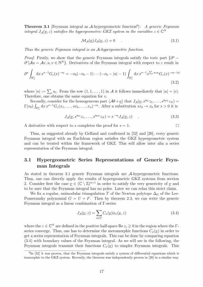
Theorem 3.1 [Feynman integral as A-hypergeometric function6]: A generic Feynmanintegral JA(ν, z) satisfies the hypergeometric GKZ system in the variables z ∈ CN
MA(ν)JA(ν, z) = 0 . (3.1)
Thus the generic Feynman integral is an A-hypergeometric function.
Proof. Firstly, we show that the generic Feynman integrals satisfy the toric part {∂u −∂v|Au = Av, u, v ∈ NN}. Derivatives of the Feynman integral with respect to z result in
∂u∫Rn+
dx xν−1Gz(x)−ν0 = −ν0(−ν0 − 1) · · · (−ν0 − |u| − 1)
∫Rn+
dx xν−1x∑i uiaiGz(x)−ν0−|u|
(3.2)
where |u| := ∑i ui. From the row (1, 1, . . . , 1) in A it follows immediately that |u| = |v|.Therefore, one obtains the same equation for v.
Secondly, consider for the homogeneous part 〈Aθ+ν〉 that JA(ν, sab1z1, . . . , sabN zN) =
Γ(ν0)∫Rn+
dx xν−1Gz(x1, . . . , sxb, . . . , xn)−ν0 . After a substitution sxb → xb for s > 0 it is
JA(ν, sab1z1, . . . , sabN zN) = s−νbJA(ν, z) . (3.3)
A derivative with respect to s completes the proof for s = 1.
Thus, as suggested already by Gelfand and confirmed in [52] and [20], every genericFeynman integral with an Euclidean region satisfies the GKZ hypergeometric systemand can be treated within the framework of GKZ. This will allow inter alia a seriesrepresentation of the Feynman integral.
3.1 Hypergeometric Series Representations of Generic Feyn-man Integrals
As stated in theorem 3.1 generic Feynman integrals are A-hypergeometric functions.Thus, one can directly apply the results of hypergeometric GKZ systems from section2. Consider first the case ν ∈ (C \ Z)n+1 in order to satisfy the very genericity of ν andto be sure that the Feynman integral has no poles. Later we can relax this strict claim.
We fix a regular, unimodular triangulation T of the Newton polytope ∆G of the Lee-Pomeransky polynomial G = U + F . Then by theorem 2.3, we can write the genericFeynman integral as a linear combination of Γ-series
JA(ν, z) =∑σ∈T
Cσ(ν)φσ(ν, z) (3.4)
where the z ∈ CN are defined in the positive half-space Re zi ≥ 0 in the region where the Γ-series converge. Thus, one has to determine the meromorphic functions Cσ(ν) in order toget a series representation of Feynman integrals. This can be done by comparing equation(3.4) with boundary values of the Feynman integral. As we will see in the following, theFeynman integrals transmit their functions Cσ(ν) to simpler Feynman integrals. This
6In [52] it was proven, that the Feynman integrals satisfy a system of differential equations which isisomorphic to the GKZ system. Recently, the theorem was independently proven in [20] in a similar way.
17
enables us to reduce Feynman integrals to the case described in corollary 1.3 and derivean analytic expression of the functions Cσ(ν).
For this purpose, consider a generic Feynman integral JA with a Newton polytopeP = ∆G = Conv(A), consisting of the vertices a1, . . . , aN , and an unimodular triangu-lation T = {σ1, . . . , σr, η1, . . . , ηs} of P . Furthermore, let T ′ = {σ1, . . . , σr} be a propersubtriangulation of T . Denote the vertices of the convex polytope P ′, which correspondto the subtriangulation T ′, by a1, . . . , aM with M < N and the corresponding Feynmanintegral7 by J ′A′ . Thus, in the second Feynman integral some monomials in Gz are missing
J ′A′(ν, z1, . . . , zM) = limzM+1,...,zN→0
JA(ν, z1, . . . , zN) . (3.5)
Applying the results from the previous sections to both Feynman integrals independentlyone obtains on the one hand
JA(ν, z1, . . . , zN) =r∑i=1
Cσi(ν)φσi(ν, z1, . . . , zN) +s∑i=1
Cηi(ν)φηi(ν, z1, . . . , zN) (3.6)
with the Γ-series
φσi(ν, z1, . . . , zN) = z−Aσiνσi
∑λ∈N|σi|0
zλσiz−AσiAσiλσi
λ!(1−Aσiν)−AσiAσiλi = 1, . . . , r (3.7)
φηi(ν, z1, . . . , zN) = z−Aηiνηi
∑λ∈N|ηi|0
zληiz−AηiAηiληi
λ!(1−Aηiν)−AηiAηiλi = 1, . . . , s (3.8)
and on the other hand
J ′A′(ν, z1, . . . , zM) =r∑i=1
C ′σi(ν)φ′σi(ν, z1, . . . , zM) (3.9)
with
φ′σi(ν, z1, . . . , zM) = z−A′σiνσi
∑λ∈N|σi|0
zλσiz−A′σiA
′σiλ
σi
λ!(1−A′σiν)−A′σiA′σiλ
i = 1, . . . , r . (3.10)
Due to the construction it is aM+1, . . . , aN ∈⋃ri=1 σi. Therefore, in the limit zM+1, . . . , zN →
0 only some zσ will be affected and it is simply
limzM+1,...,zN→0
φσi(ν, z1, . . . , zN) = φ′σi(ν, z1, . . . , zM) . (3.11)
Apart from that, as a consequence of the homogeneous differential equations 〈Aθ +ν〉 all solutions of a GKZ hypergeometric system have to satisfy the scaling propertyφ(ν, sz) = s−ν0φ(ν, z). It can be easily seen that Γ-series satisfy this property. In thepower series part of a Γ-series the variables z only appear as ratios, such that they are
scaling invariant (in accordance with lemma 6.3). However, the monomial z−A−1
η νη in front
7J ′A′ is not necessarily a Feynman integral coming from an actual Feynman graph. It is sufficient, thatJ ′A′ has the shape of an Euler-Mellin integral described in definition 1.2. Thus, G′z can be an arbitrarynon-homogeneous polynomial.
18
of the power series will give the scaling property since s∑i∈η(−A−1
η ν)i = s−ν0 according tolemma 6.3.
Since in every Γ-series φηi some of the variables zM+1 . . . , zN are contained in themonomial, the scaling property will be violated in the limit zM+1 . . . , zN → 0. Thus, thefunctions limzM+1,...zN→0 φηi can not be linearly dependent of {φ′σi}. Since one already hasr linearly independent solutions φ′σi and therewith has a full-dimensional solution spacefor the Feynman integral J ′A′ , the Γ-series φηi have to vanish
limzM+1,...,zN→0
φηi(ν, z1, . . . , zN) = 0 . (3.12)
Thus, the GKZ systems behave naturally, as also mentioned in [26]: If one deletes avertex of Conv(A), the Γ-series which correspond to simplices containing this vertex willvanish. This leads to a very simple connection between subtriangulations of Feynmanintegrals. Applying the limit zM+1, . . . , zN → 0, the meromorphic functions Cσ(ν) willnot be affected and one obtains Cσi(ν) = C ′σi(ν).
Thus, one can determine the meromorphic functions Cσ(ν) by considering simplerFeynman integrals which refer to subtriangulations, where by a simpler Feynman integralwe mean a Feynman integral where the Lee-Pomeransky polynomial G has less monomials.In this way one can define ancestors and descendants of Feynman integrals by deletingor adding monomials to the Lee-Pomeransky polynomial G. E.g. the massless one-loopbubble graph is a descendant of the one-loop bubble graph with one mass, which itselfis a descendant of the full massive one-loop bubble. Those ancestors and descendants donot necessarily correspond to Feynman integrals in the original sense, since one can alsoconsider polynomials G which are not connected to graph polynomials anymore.
As a trivial subtriangulation of an arbitrary triangulation one can choose one of itssimplices. In doing so, one can relate the prefactors Cσ(ν) to the problem where onlyone simplex is involved. For such problems, one can solve the Feynman integral easily asseen in corollary 1.3. Therefore, for an unimodular triangulation one can find that theprefactors are simply given by
Cσ(ν) = Γ(A−1σ ν) (3.13)
which results in the following theorem:
Theorem 3.2 [Series representation of Feynman integrals]: Let T be a regular, uni-modular triangulation of the Newton polytope ∆G = Conv(A) corresponding to a genericFeynman integral JA. Then the generic Feynman integral can be written as
JA(ν, z) =∑σ∈T
z−A−1σ ν
σ
∑λ∈N|σ|0
Γ(A−1σ ν +A−1
σ Aσλ)
λ!
zλσ(−zσ)A
−1σ Aσλ
(3.14)
where the series have a common region of convergence. This representation holds forgeneric ν ∈ Cn+1, which means that ν has to be chosen such that the Feynman integralhas no poles and none of the power series in (3.14) will be identical to zero.
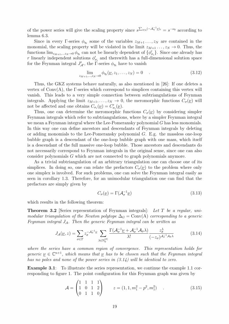
Example 3.1: To illustrate the series representation, we continue the example 1.1 cor-responding to figure 1. The point configuration for this Feynman graph was given by
A =
1 1 1 11 0 1 20 1 1 0
z = (1, 1,m21 − p2,m2
1) . (3.15)
19
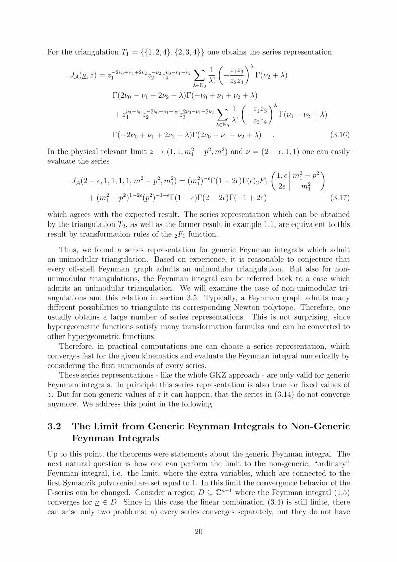
For the triangulation T1 = {{1, 2, 4}, {2, 3, 4}} one obtains the series representation
JA(ν, z) = z−2ν0+ν1+2ν21 z−ν2
2 zν0−ν1−ν24
∑λ∈N0
1
λ!
(−z1z3
z2z4
)λΓ(ν2 + λ)
Γ(2ν0 − ν1 − 2ν2 − λ)Γ(−ν0 + ν1 + ν2 + λ)
+ zν2−ν04 z−2ν0+ν1+ν2
2 z2ν0−ν1−2ν23
∑λ∈N0
1
λ!
(−z1z3
z2z4
)λΓ(ν0 − ν2 + λ)
Γ(−2ν0 + ν1 + 2ν2 − λ)Γ(2ν0 − ν1 − ν2 + λ) . (3.16)
In the physical relevant limit z → (1, 1,m21 − p2,m2
1) and ν = (2 − ε, 1, 1) one can easilyevaluate the series
JA(2− ε, 1, 1, 1, 1,m21 − p2,m2
1) = (m21)−εΓ(1− 2ε)Γ(ε)2F1
(1, ε
2ε
∣∣∣∣ m21 − p2
m21
)+ (m2
1 − p2)1−2ε(p2)−1+εΓ(1− ε)Γ(2− 2ε)Γ(−1 + 2ε) (3.17)
which agrees with the expected result. The series representation which can be obtainedby the triangulation T2, as well as the former result in example 1.1, are equivalent to thisresult by transformation rules of the 2F1 function.
Thus, we found a series representation for generic Feynman integrals which admitan unimodular triangulation. Based on experience, it is reasonable to conjecture thatevery off-shell Feynman graph admits an unimodular triangulation. But also for non-unimodular triangulations, the Feynman integral can be referred back to a case whichadmits an unimodular triangulation. We will examine the case of non-unimodular tri-angulations and this relation in section 3.5. Typically, a Feynman graph admits manydifferent possibilities to triangulate its corresponding Newton polytope. Therefore, oneusually obtains a large number of series representations. This is not surprising, sincehypergeometric functions satisfy many transformation formulas and can be converted toother hypergeometric functions.
Therefore, in practical computations one can choose a series representation, whichconverges fast for the given kinematics and evaluate the Feynman integral numerically byconsidering the first summands of every series.
These series representations - like the whole GKZ approach - are only valid for genericFeynman integrals. In principle this series representation is also true for fixed values ofz. But for non-generic values of z it can happen, that the series in (3.14) do not convergeanymore. We address this point in the following.
3.2 The Limit from Generic Feynman Integrals to Non-GenericFeynman Integrals
Up to this point, the theorems were statements about the generic Feynman integral. Thenext natural question is how one can perform the limit to the non-generic, “ordinary”Feynman integral, i.e. the limit, where the extra variables, which are connected to thefirst Symanzik polynomial are set equal to 1. In this limit the convergence behavior of theΓ-series can be changed. Consider a region D ⊆ Cn+1 where the Feynman integral (1.5)converges for ν ∈ D. Since in this case the linear combination (3.4) is still finite, therecan arise only two problems: a) every series converges separately, but they do not have
20
a common convergence region anymore or b) some of the Γ-series diverge, but the linearcombination is still finite. In the first case a) the convergence criteria for the variables
of the Γ-series xj = (zσ)j∏
i(zσ)−(A−1
σ Aσ)iji exclude each other for different σ ∈ T . In the
second case b) the variables xj become constants after the limit (usually equals 1), whichcan be outside of the convergence region.
Because of these possible issues, it can be difficult to perform the limit. Fortunatelythere is a strategy to tackle these problems in many cases by transformation formulas ofhypergeometric functions. E.g. for the 2F1 hypergeometric function, there is a well knowntransformation formula [56]
2F1
(a, b
c
∣∣∣∣ z) =Γ(c)Γ(c− a− b)Γ(c− a)Γ(c− b)2F1
(a, b
a+ b− c+ 1
∣∣∣∣ 1− z)+ (1− z)c−a−b
Γ(c)Γ(a+ b− c)Γ(a)Γ(b)
2F1
(c− a, c− bc− a− b+ 1
∣∣∣∣ 1− z) , (3.18)
which can be applied to change a limit xj → 1 to the much simpler case of a limit xj → 0.We illustrate this method with an example. For the 2-loop sunset graph with two differentmasses, inter alia there appears the hypergeometric series
φ2 =∑k∈N4
0
(1− ε)k3+k4(ε)k1+2k2+k3(ε− 1)−k1−k2+k4(2− 2ε)k1−k3−k4
1
k1!k2!k3!k4!
(−z1z6
z5z2
)k1(−z4z6
z25
)k2(−z2z7
z3z5
)k3(−z2z8
z3z6
)k4
(3.19)
where one has to consider the limit (z1, z2, z3, z4, z5, z6, z7, z8) → (1, 1, 1,m22,m
21 + m2
2 −p2
1,m21,m
22,m
21). In this limit it appears the term (−1)k4 , which is not in the convergence
region for small values of ε > 0 anymore. Therefore, we evaluate the k4 series carefullyand write
φ2 = limt→1
∑(k1,k2,k3)∈N3
0
(1− ε)k3(ε− 1)−k1−k2(2− 2ε)k1−k3(ε)k1+2k2+k3
1
k1!k2!k3!
(−x1)k1 (−x1x2)k2 (−x2)k32F1
(−ε+ k3 + 1, ε− k1 − k2 − 1
2ε− k1 + k3 − 1
∣∣∣∣ t) (3.20)
where xi =m2i
m21+m2
2−p21. With the transformation formula for the 2F1 function, one can split
the series in a convergent and a divergent part
φ2 =∑
(k1,k2,k3)∈N30
Γ(k2 + 2ε− 1)Γ(−k1 + k3 + 2ε− 1)
Γ(−k1 + 3ε− 2)Γ(k2 + k3 + ε)(1− ε)k3(ε− 1)−k1−k2(2− 2ε)k1−k3
(ε)k1+2k2+k3
1
k1!k2!k3!(−x1)k1(−x2)k3(−x1x2)k2 + lim
t→1
∑(k1,k2,k3,k4)∈N4
0
(1− t)k2+k4+2ε−1
k1!k2!k3!k4!
Γ(−k2 − 2ε+ 1)Γ(−k1 + k3 + 2ε− 1)Γ(k2 + k3 + ε+ k4)Γ(k2 + 2ε)Γ(−k1 + 3ε− 2 + k4)
Γ(k3 − ε+ 1)Γ(−k1 − k2 + ε− 1)Γ(k2 + k3 + ε)Γ(k2 + 2ε+ k4)Γ(−k1 + 3ε− 2)
(ε)k1+2k2+k3(1− ε)k3(ε− 1)−k1−k2(2− 2ε)k1−k3(−x1)k1(−x2)k3(−x1x2)k2
21
=∑
(k1,k2,k3)∈N30
Γ(k2 + 2ε− 1)Γ(−k1 + k3 + 2ε− 1)
Γ(−k1 + 3ε− 2)Γ(k2 + k3 + ε)(1− ε)k3(ε− 1)−k1−k2(2− 2ε)k1−k3
(ε)k1+2k2+k3
1
k1!k2!k3!(−x1)k1(−x2)k3(−x1x2)k2 + lim
t→1(1− t)2ε−1
∑(k1,k3)∈N2
0
(−x1)k1(−x2)k3
k1!k3!
Γ(−2ε+ 1)Γ(−k1 + k3 + 2ε− 1)
Γ(1− ε)Γ(ε− 1)(ε)k1+k3(2− 2ε)k1−k3 . (3.21)
Comparing the divergent part with the other Γ-series, which occurs in the calcula-tion of the sunset graph with two masses, one can find another divergent series whichexactly cancels this divergence. This cancellation has always to happen, since the linearcombination has to be finite.
Therefore, one can derive a convergent series representation also for non-generic Feyn-man integrals by considering convenient transformation formulas of hypergeometric func-tions. In principle, this procedure will work in general, but it can be necessary to involvemore complicated transformation formulas than the well-studied 2F1 transformation andalso the cancellation of the divergences may be not so obvious as in this case. Fortunately,many graphs (also for L > 1) can even be evaluated with the transformation formula ofthe 2F1 function.
In fact, this limit can reduce the dimension of the solution space, which is the expectedbehavior. For generic variables z ∈ CN the dimension of the solution space is equal tovol0 ∆G according to theorem 2.2. In contrast for non-generic values of z ∈ CN thedimension of the solution space is equal to the Euler characteristic (−1)nχ((C?)n \ {G =0}) [6], which is in general smaller or equal to the volume of the Newton polytope
(−1)nχ((C?)n \ {G = 0}) ≤ vol0 ∆G . (3.22)
Thus, by calculating the Euler characteristic we can count the expected dependencies inthe limit from generic to non-generic Feynman integrals. According to [6] it is mean-ingful to define the number of master integrals as the dimension of the solution space.Therefore, one can see the linear combination of Γ-series (3.4) as a procedure similar to adecomposition of a general Feynman integral into a basis of master integrals. This anal-ogy mirrors also the existence of different decompositions (which corresponds to differenttriangulations) and their transformation into each other by shift relations [47].
3.3 The ε Expansion of Hypergeometric Series Representations
In the calculus of dimensional regularization [73] one is usually interested in the Laurentexpansion of the Feynman integrals around ε = 0 where d = 4−2ε. Due to the theorem 1.5one can relate this task to the Taylor expansion of the hypergeometric series representa-tion. Thus, one has simply to differentiate the Horn hypergeometric series. As pointed outin [16], the derivatives with respect to parameters of Horn hypergeometric series are againHorn hypergeometric series of higher degree. By the identities (a)m+n = (a)m(a + m)nand (a)rn = rrn
∏r−1j=0
(a+jr
)n
for r ∈ Z>0 one can reduce all derivatives to two cases [16]
∂
∂a
∞∑n=0
B(n)(a)nxn = x
∞∑k=0
∞∑n=0
B(n+ k + 1)(a+ 1)n+k(a)k
(a+ 1)kxn+k (3.23)
∂
∂a
∞∑n=0
B(n)(a)−nxn = −x
∞∑k=0
∞∑n=0
B(n+ k + 1)(a)−n−k−1(a)−k−1
(a)−kxn+k . (3.24)
22
Thus, Horn hypergeometric functions do not only appear as solutions of Feynman integralswith unimodular triangulations, but also in every coefficient of the Laurent expansionof those Feynman integrals. Therefore, the class of Horn hypergeometric functions issufficient to describe almost all Feynman integrals and their Laurent expansion. Hence, itis not surprising that also the combinatorial structure of Feynman integrals is reflected inthe Horn hypergeometric functions. For instance, the relations between different Feynmanintegrals can be derived by transformation formulas of hypergeometric functions and viceversa [47].
Another way to expand the Horn hypergeometric functions around ε = 0 in some casescould be the approach of S- and Z-sums [50], which are related to multiple polylogarithmsand related functions. Unfortunately, many examples, which can be generated by the GKZapproach, belong not to the known algorithms given in [50].
3.4 Applications to other Parametric Representations
The GKZ mechanism with the resulting series representation used above is not limited tothe Feynman integral in the Lee-Pomeransky representation. It is a method which canbe used for all integrals of Euler-Mellin type including one polynomial. Thus, there aremore applications in the Feynman integral calculus. For example the Feynman parametricrepresentation (1.3) is of that form, if either the first Symanzik polynomial U or the secondSymanzik polynomial F drops out.
This is the case e.g. for all 1-loop Feynman integrals, where the first Symanzik poly-nomial U evaluates to 1 after applying the δ-function. With νn = 1 after one integrationthe Feynman integral is of the form of an Euler-Mellin integral
∫Rn−1
+dx xν−1F−ω, where
we denote x = (x1, . . . , xn−1), ν = (ν1, . . . , νn−1) and F = F |xn→1−∑n−1i=1 xi
. Also for so
called “marginal” Feynman integrals [9], where ω = d/2, the first Symanzik polynomialdrops out of the representation (1.3) and one obtains the integral
∫Rn−1
+dx xν−1F−d/2. For
instance all “banana”-graphs are marginal for νi = 1 and d = 2.In contrast the second Symanzik polynomial drops out for ω = 0, which is the well-
studied case of periods (e.g. [12])∫Rn−1
+dx xν−1U−d/2. Note that this integral is highly
non-generic from the perspective of the GKZ approach. Thus, the case where the secondSymanzik polynomial F remains is usually much easier, since one has not to introduceextra variables in the first Symanzik polynomial U .
Last but not least, also the Baikov representation [6, 33] is a possible candidate toapply the GKZ approach as well.
3.5 Non-Unimodular Triangulations of Feynman Polytopes
The treatments above were specialized to unimodular triangulations only. This strategyhas various reasons. Without much effort, one could extend theorem 2.3 also to the case ofnon-unimodular triangulations and write the Feynman integral as a linear combination ofΓ-series as in equation (3.4). In contrast, for a non-unimodular triangulation one can notdetermine the meromorphic functions Cσ(ν) such as easy as in theorem 3.2. Nevertheless,one can reduce Feynman integrals without unimodular triangulations to subtriangulationsas described in section 3.1.
However, after checking common Feynman integrals up to three loops, we are leadedto the conjecture that all off-shell Feynman graphs admit at least one unimodular triangu-
23

lation. This conjecture seems also likely by considering the very specific form of Newtonpolytopes ∆G arising in Feynman integrals (lemma 6.2).
In contrast some on-shell graphs do not admit an unimodular triangulation. Forinstance the on-shell full massive 1-loop bubble with G = x1 + x2 + m2
1x21 + m2
2x22 does
not allow an unimodular triangulation. However, since the off-shell fully massive 1-loopbubble admits unimodular triangulations, one can treat the on-shell Feynman integral asa limit of the off-shell version.
This behavior holds in general: one can always add monomials to the Lee-Pomeranskypolynomial G→ G′, such that the Newton polytope ∆G′ admits an unimodular triangu-lation. This can be seen by a result of Knudsen et al. [46]:
Lemma 3.3 [[13, 46]]: For every lattice polytope P there is an integer k ∈ N such thatthe dilated polytope kP := {kµ|µ ∈ P} admits an unimodular triangulation.
Thus, if the Newton polytope ∆G of a Feynman integral does not admit an unimod-ular triangulation, one can dilate the polytope ∆G until the polytope k∆G admits anunimodular triangulation. Then the original Feynman integral can be obtained as a limitwhere all additional vertices vanish and where we scale the propagator powers by k andthe whole integral by kn
JA(ν, z) = knΓ(ν0)
∫Rn+
dx xkν−1Gz(xk)−ν0 . (3.25)
Thus, one can always write the Feynman integral as a limit of another integral where itsNewton polytope allows an unimodular triangulation. That is the reason, why we canfocus only on the unimodular triangulations and vindicates the procedure above.
4 Advanced Example: Full Massive Sunset
To illustrate the GKZ method stated above, as well as to show the power of this approach,we calculate a series representation of the sunset Feynman integral with three differentmasses according to figure 3. The corresponding Feynman graph consists in n = 3 edgesand the Lee-Pomeransky polynomial includes N = 10 monomials
G = x1x2 + x1x3 + x2x3 + (m21 +m2
2 +m23 − p2)x1x2x3
+m21x
21(x2 + x3) +m2
2x22(x1 + x3) +m2
3x23(x1 + x2) . (4.1)
p
m1
m2
m3
p
Figure 3: The 2-loop 2-point function (sunset graph) with three different masses.
24
In the representation of equation (1.7) we encode this polynomial by
A =
1 1 1 1 1 1 1 1 1 10 1 1 0 1 0 1 2 1 21 0 1 1 0 2 1 0 2 11 1 0 2 2 1 1 1 0 0
(4.2)
z = (1, 1, 1,m23,m
23,m
22,m
21 +m2
2 +m23 − p2
1,m21,m
22,m
21) . (4.3)
The rank of the kernel of A is equal to r = N − n − 1 = 6 and therefore we willexpect 6-dimensional Γ-series. Moreover, the polytope ∆G = Conv(A) has the volumevol0(Conv(A)) = 10 (calculated with polymake [25]), which leads to 10 basis solutions, andthere are 826 different ways for a regular triangulation of the Newton polytope ∆G, where466 of those triangulations are unimodular. We choose the unimodular triangulation(calculated with TOPCOM [59])
T152 = {{3, 6, 7, 9}, {3, 7, 9, 10}, {3, 7, 8, 10}, {2, 5, 7, 8}, {2, 3, 7, 8},{2, 4, 5, 7}, {1, 4, 6, 7}, {1, 2, 4, 7}, {1, 3, 6, 7}, {1, 2, 3, 7}} (4.4)
in order to get series, which converge fast for highly relativistic kinematics m2i � m2
1 +m2
2 +m23 − p2. Further, we set νi = 1 and d = 4− 2ε.
In the limit z → (1, 1, 1,m23,m
23,m
22,m
21 + m2
2 + m23 − p2
1,m21,m
22,m
21) the series φ1,
φ3, φ5, φ6, φ8 and φ9 are divergent for small values of ε > 0. By the method describedin section 3.2 one can split all these series by the transformation formula for the 2F1
hypergeometric function in a convergent and a divergent part. The divergent parts ofthese series cancel each other. In doing so the resulting Γ-series have linear dependencesand the dimension of the solution space will reduce from 10 to 7.
By applying all these steps one arrives at the following series representation of the fullmassive sunset integral
IA(ν, z) =s1−2ε
Γ(3− 3ε)
[x1−ε
2 φ1 + (x1x2)1−εφ2 + x1−ε1 φ3 + (x1x3)1−εφ4 + x1−ε
1 φ5
+x1−ε3 φ6 + (x2x3)1−εφ7 + x1−ε
3 φ8 + x1−ε2 φ9 + φ10
](4.5)
where the Γ-series are given by
φ1 =∞∑
k2,k3,k4,k5,k6=0
(−x2)k2(−x3)k3(−x2x3)k4(−x1x2)k5(−x1)k6
k2!k3!k4!k5!k6!
Γ(k2 − 3ε+ 3)Γ(k2 + k3 + k4 − k6 − 2ε+ 3)Γ(k3 − k5 − k6 − ε+ 1)
Γ(k2 + k3 + 2k4 + 2k5 + k6 + ε)Γ(k4 + k5 + 2ε− 1)Γ(−k2 − k3 − k4 + k6 + 2ε− 2)
Γ(k2 + k4 + k5 − ε+ 2)Γ(k3 + k4 − k6 + ε)
φ2 =∞∑
k1,k2,k3,k4,k5,k6=0
(−x1)k1+k5(−x2)k2+k6(−x1x3)k3(−x2x3)k4
k1!k2!k3!k4!k5!k6!
Γ(k1 + k2 + 2k3 + 2k4 + k5 + k6 + 1)Γ(k1 + k2 − 3ε+ 3)
Γ(−k2 − k4 + k5 − k6 + ε− 1)Γ(−k1 − k3 − k5 + k6 + ε− 1)
φ3 =∞∑
k1,k3,k4,k5,k6=0
(−x1)k1(−x1x3)k3(−x3)k4(−x1x2)k5(−x2)k6
k1!k3!k4!k5!k6!
Γ(k1 − 3ε+ 3)Γ(k1 + k3 + k4 − k6 − 2ε+ 3)Γ(k4 − k5 − k6 − ε+ 1)
Γ(k1 + 2k3 + k4 + 2k5 + k6 + ε)Γ(k3 + k5 + 2ε− 1)Γ(−k1 − k3 − k4 + k6 + 2ε− 2)
Γ(k1 + k3 + k5 − ε+ 2)Γ(k3 + k4 − k6 + ε)
25
φ4 =∞∑
k1,k2,k3,k4,k5,k6=0
(−x1)k1+k3(−x3)k2+k6(−x1x2)k4(−x2x3)k5
k1!k2!k3!k4!k5!k6!
Γ(k1 + k2 + k3 + 2k4 + 2k5 + k6 + 1)Γ(k1 + k2 − 3ε+ 3)
Γ(−k2 + k3 − k5 − k6 + ε− 1)Γ(−k1 − k3 − k4 + k6 + ε− 1)
φ5 =∞∑
k1,k2,k3,k4,k5=0
(−x1)k1(−x1x3)k2(−x3)k3(−x1x2)k4(−x2)k5
k1!k2!k3!k4!k5!
Γ(k1 + k2 + k3 − k5 − 2ε+ 2)Γ(−k2 − k3 + k5 − ε+ 1)Γ(−k1 − k2 − k4 + ε− 1)
Γ(k1 + 2k2 + k3 + 2k4 + k5 + ε)Γ(k2 + k4 + 2ε− 1)Γ(−k1 − k2 − k3 + k5 + 2ε− 1)
Γ(−k3 + k4 + k5 + ε)Γ(−k1 + 3ε− 2)
φ6 =∞∑
k2,k3,k4,k5,k6=0
(−x3)k2(−x2)k3(−x1)k4(−x2x3)k5(−x1x3)k6
k2!k3!k4!k5!k6!
Γ(k2 − 3ε+ 3)Γ(k2 + k3 − k4 + k5 − 2ε+ 3)Γ(k3 − k4 − k6 − ε+ 1)
Γ(k2 + k3 + k4 + 2k5 + 2k6 + ε)Γ(−k2 − k3 + k4 − k5 + 2ε− 2)Γ(k5 + k6 + 2ε− 1)
Γ(k2 + k5 + k6 − ε+ 2)Γ(k3 − k4 + k5 + ε)
φ7 =∞∑
k1,k2,k3,k4,k5,k6=0
(−x2)k1+k3(−x3)k2+k5(−x1x2)k4(−x1x3)k6
k1!k2!k3!k4!k5!k6!
Γ(k1 + k2 + k3 + 2k4 + k5 + 2k6 + 1)Γ(k1 + k2 − 3ε+ 3)
Γ(−k1 − k3 − k4 + k5 + ε− 1)Γ(−k2 + k3 − k5 − k6 + ε− 1)
φ8 =∞∑
k1,k3,k4,k5,k6=0
(−x3)k1(−x2)k3(−x1)k4(−x2x3)k5(−x1x3)k6
k1!k3!k4!k5!k6!
Γ(k1 + k3 − k4 + k5 − 2ε+ 2)Γ(−k3 + k4 − k5 − ε+ 1)Γ(−k1 − k5 − k6 + ε− 1)
Γ(k1 + k3 + k4 + 2k5 + 2k6 + ε)Γ(−k1 − k3 + k4 − k5 + 2ε− 1)Γ(k5 + k6 + 2ε− 1)
Γ(−k3 + k4 + k6 + ε)Γ(−k1 + 3ε− 2)
φ9 =∞∑
k1,k2,k3,k4,k6=0
(−x2)k1(−x3)k2(−x2x3)k3(−x1x2)k4(−x1)k6
k1!k2!k3!k4!k6!
Γ(k1 + k2 + k3 − k6 − 2ε+ 2)Γ(−k2 − k3 + k6 − ε+ 1)Γ(−k1 − k3 − k4 + ε− 1)
Γ(k1 + k2 + 2k3 + 2k4 + k6 + ε)Γ(k3 + k4 + 2ε− 1)Γ(−k1 − k2 − k3 + k6 + 2ε− 1)
Γ(−k2 + k4 + k6 + ε)Γ(−k1 + 3ε− 2)
φ10 =∞∑
k1,k2,k3,k4,k5,k6=0
(−x3)k1+k2(−x2)k3+k5(−x1)k4+k6
k1!k2!k3!k4!k5!k6!
Γ(k2 − k3 + k4 − k5 − ε+ 1)Γ(k1 + k3 − k4 − k6 − ε+ 1)
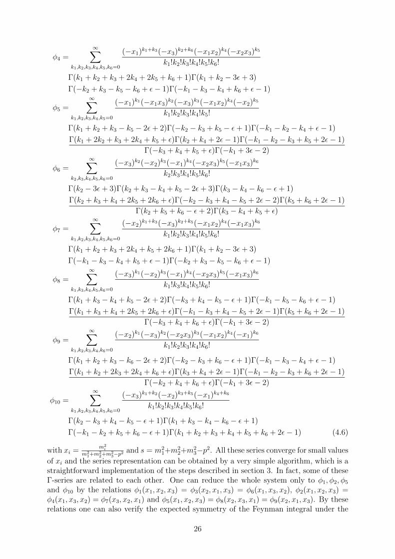
Γ(−k1 − k2 + k5 + k6 − ε+ 1)Γ(k1 + k2 + k3 + k4 + k5 + k6 + 2ε− 1) (4.6)
with xi =m2i
m21+m2
2+m23−p2 and s = m2
1+m22+m2
3−p2. All these series converge for small values
of xi and the series representation can be obtained by a very simple algorithm, which is astraightforward implementation of the steps described in section 3. In fact, some of theseΓ-series are related to each other. One can reduce the whole system only to φ1, φ2, φ5
and φ10 by the relations φ1(x1, x2, x3) = φ3(x2, x1, x3) = φ6(x1, x3, x2), φ2(x1, x2, x3) =φ4(x1, x3, x2) = φ7(x3, x2, x1) and φ5(x1, x2, x3) = φ8(x2, x3, x1) = φ9(x2, x1, x3). By theserelations one can also verify the expected symmetry of the Feynman integral under the
26
permutation x1 ↔ x2 ↔ x3.In order to expand the Feynman integral IA for small values of ε > 0 one can use the
methods described in section 3.3 or alternatively by expanding each Γ-function separately.The latter requires to distinguish between positive and negative integers in the argumentof the Γ-function
Γ(bε+ n)n∈Z≥1
= Γ(n)
[1 + bεψ0(n) +
b2ε2
2
(ψ0(n)2 + ψ1(n)
)+b3ε3
6
(ψ0(n)3 + 3ψ0(n)ψ1(n) + ψ2(n)
)+O
(ε4)]
Γ(bε+ n)n∈Z≤0
=(−1)n
Γ(−n+ 1)
[1
bε+ ψ0(1− n) +
bε
2
(2ζ2 + ψ0(1− n)2 − ψ1(1− n)
)+b2ε2
6
(ψ0(1− n)3 + 6ζ2ψ0(1− n)− 3ψ0(1− n)ψ1(1− n) + ψ2(1− n)
)+O
(ε3)]
.
(4.7)
By the distinction of cases between positive and negative arguments in the Γ functionsmany terms arise, which are easily manageable by a CAS but which are space-consumingin print, wherefore we omit to state these results here. The correctness of these resultswas checked numerically by FIESTA [67] with arbitrary kinematics and masses, satisfyingxi < 0.5. For small values of xi the resulting series converges fast, such that for a goodapproximation one only has to take the first summands into account. An upper boundfor the errors in a finite summation can be estimated by a majorant geometric series,similar to the procedure in theorem 6.6. Vice versa one can determine the number ofrequired summands for a given error bound. Furthermore, the summands of a Hornhypergeometric series always have a rational ratio. Thus, in a numerical calculation oneonly has to evaluate rational functions. In this way Horn hypergeometric series have arelatively simple and controllable numerical behavior in the case |xi| � 1.
5 Conclusion and Outlook
We showed in this article that Feynman integrals can be described as hypergeometric func-tions. Namely we showed that a) every generic Feynman integral is an A-hypergeometricfunction, that b) every generic Feynman integral which admits a regular, unimodular tri-angulation has a representation in Horn hypergeometric functions and that c) all scalar,dimensional regularizable and Euclidean Feynman integrals can be written at least as alimit of a linear combination of Horn hypergeometric functions. Furthermore, the latter(c) is also true for all coefficients in a Laurent expansion of the Feynman integral in adimensional or analytic regularization.
Since hypergeometric functions are mostly represented in terms of integrals includingpolynomials, Mellin-Barnes integrals including Γ-functions or series including Pochham-mer symbols, it is not surprising that also Feynman integrals appear normally in one ofthose representations. From the perspective of general hypergeometric functions the com-mon ground of these representations is an integer matrix A ∈ Z(n+1)×N or equivalentlya Newton polytope ∆G = Conv(A). By the triangulation of this Newton polytope wederived an analytic formula for a hypergeometric series representation of the Feynmanintegral. As there are in general many different ways to triangulate a polytope, thereare also many different series representations possible. Similar to the Feynman integral
27
those hypergeometric series satisfy different relations between each other and can there-fore also be transformed in equivalent representations. However, the series representationscan differ in their convergence behavior. Thus, there can be series representations whichconverge fast for given kinematics so that we sometimes only need the first summands inorder to reach a high precision numerical approximation.
For the purpose of a practical usage of this concept, we discussed possible obstacleswhich can appear in the concrete evaluation and gave some strategies to solve them. Theprocedure described in section 3 and illustrated in section 4 works similarly in all casesand can be read as an algorithm.
Besides numerical applications, there are structurally interesting implications for theFeynman integral. Since in both subjects similar questions appear, the hypergeomet-ric perspective opens new ways to analyze the Feynman integral. For instance the sin-gularities of hypergeometric functions, and therefore simultaneously the singularities ofFeynman integrals, are given by the A-discriminants and the coamoebas.
The series representation given in the present work, is only one of many consequencesthat we can obtain by the connection between Feynman integrals and hypergeometricfunctions. On the one hand we outlined in section 3.4 that we also can apply the GKZapproach to other integrals appearing in the Feynman calculus. On the other hand onecan also solve the GKZ system with other functions to obtain representations of theFeynman integral e.g. in terms of other integrals. This leads us to the question, if onecan relate Feynman integrals with the GKZ approach to other Feynman integrals in aconsistent way, in order to get linear relations between Feynman integrals similar to theIBP approach.
Furthermore, it would be desirable to get a better understanding of the relationsbetween Feynman integrals and their diagrams sharing parts of the matrices A. Thesimplest connection between those Feynman integrals are the ancestors and descendantsof Feynman integrals mentioned in section 3.1. Lastly, we leave several technical questionsopen to solve in future work. For instance, a proof of the conjecture that off-shell Feynmanintegrals always admit unimodular triangulations together with a better understanding ofthe behavior in non-generic cases as described in section 3.2, would show that all off-shellFeynman integrals can be written as Horn hypergeometric functions and not only as alimit of Horn hypergeometric functions.
In this article we suggested a new perspective of an old idea to characterize Feynmanintegrals. This hypergeometric perspective can be useful for practical computation butalso for a better conceptual understanding of Feynman integrals. Still, this is merely astarting point for future research on the correspondence between Feynman integrals andhypergeometric functions in the GKZ theory.
28
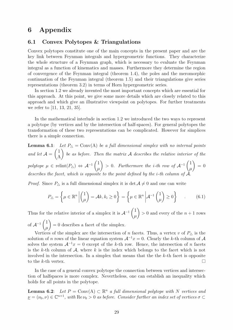
6 Appendix
6.1 Convex Polytopes & Triangulations
Convex polytopes constitute one of the main concepts in the present paper and are thekey link between Feynman integrals and hypergeometric functions. They characterizethe whole structure of a Feynman graph, which is necessary to evaluate the Feynmanintegral as a function of kinematics and masses. Furthermore they determine the regionof convergence of the Feynman integral (theorem 1.4), the poles and the meromorphiccontinuation of the Feynman integral (theorem 1.5) and their triangulations give seriesrepresentations (theorem 3.2) in terms of Horn hypergeometric series.
In section 1.2 we already invented the most important concepts which are essential forthis approach. At this point, we give some more details which are closely related to thisapproach and which give an illustrative viewpoint on polytopes. For further treatmentswe refer to [11, 13, 21, 35].
In the mathematical interlude in section 1.2 we introduced the two ways to representa polytope (by vertices and by the intersection of half-spaces). For general polytopes thetransformation of these two representations can be complicated. However for simplicesthere is a simple connection.
Lemma 6.1: Let P4 = Conv(A) be a full dimensional simplex with no internal points
and let A =
(1A
)be as before. Then the matrix A describes the relative interior of the
polytope µ ∈ relint(P4) ⇔ A−1
(1µ
)> 0. Furthermore the i-th row of A−1
(1µ
)= 0
describes the facet, which is opposite to the point defined by the i-th column of A.
Proof. Since P4 is a full dimensional simplex it is detA 6= 0 and one can write
P4 =
{µ ∈ Rn
∣∣∣∣(1µ
)= Ak, ki ≥ 0
}=
{µ ∈ Rn
∣∣∣∣A−1
(1µ
)≥ 0
}. (6.1)
Thus for the relative interior of a simplex it is A−1
(1µ
)> 0 and every of the n+ 1 rows
of A−1
(1µ
)= 0 describes a facet of the simplex.
Vertices of the simplex are the intersection of n facets. Thus, a vertex v of P4 is thesolution of n rows of the linear equation system A−1x = 0. Clearly the k-th column of Asolves the system A−1x = 0 except of the k-th row. Hence, the intersection of n facetsis the k-th column of A, where k is the index which belongs to the facet which is notinvolved in the intersection. In a simplex that means that the the k-th facet is oppositeto the k-th vertex.
In the case of a general convex polytope the connection between vertices and intersec-tion of halfspaces is more complex. Nevertheless, one can establish an inequality whichholds for all points in the polytope.
Lemma 6.2: Let P = Conv(A) ⊂ Rn a full dimensional polytope with N vertices andν = (ν0, ν) ∈ Cn+1, with Re ν0 > 0 as before. Consider further an index set of vertices σ ⊂
29
{1, . . . , N} which corresponds to a simplex, detAσ 6= 0. Then the following equivalenceholds
ν/ν0 ∈ P ⇔ (A−1σ )iν ≥
N−n−1∑j=1
(A−1σ Aσ)ijrj with r ∈ RN−n−1
≥0 (6.2)
where ν/ν0 := (ν1/ν0, . . . νn/ν0) is the componentwise division.
Proof. From the vertex definition of polytopes it is
ν/ν0 ∈ P ⇔(
1ν/ν0
)= Ak ⇔ ν = Ak (6.3)
for k, k ∈ RN≥0. Since the polytope is full dimensional, there is a triangulation and one can
divide the polytope in A = (Aσ,Aσ) where Aσ has an inverse. Thus the lemma followsby multiplying by the inverse A−1
σ .
This lemma establishes a connection between the signs of the matrix A−1σ Aσ and the
geometry of the polytope. Since the signs of A−1σ Aσ determine the kinematic regions
where the series representations (theorem 3.2) converge fast, this lemma can be useful toanalyze triangulations in a numerical application.
Furthermore, the matrices Aσ and Aσ which appear in the triangulation procedurehas some special properties, which also guaranties the convergence of Γ-series.
Lemma 6.3: Let P = Conv(A) be a full dimensional polytope with integer verticesA ∈ Zn×N and T a triangulation, where the indices of the simplices are denoted by σ.Then it holds ∑
i∈σ
(A−1σ Aσ)ij = 1 (6.4)
for all j = 1, . . . , N and ∑i∈σ
(A−1σ ν)i = ν0 (6.5)
where σ is the complement of σ and ν = (ν0, ν1, . . . , νn) ∈ Cn+1 an arbitrary complexvector.
Proof. The columns of the matrix B =
(−A−1
σ Aσ1
)∈ QN×r are a basis of the lattice
L := ker(A) ∩ Z, which can be verified by direct computation AB = 0. It followsparticularly that
∑j Bjk = 0 and thereby equation (6.4). The second statement (6.5)
follows trivially from∑
j,k(Aσ)ij(A−1σ )jkνk = νi.
This lemma also implies that the appearing variables xj = (zσ)j∏
i(zσ)−(A−1
σ Aσ)iji in
the Γ-series are dimensionless (without units). Therefore, the unit of the Γ-series will beonly determined by the monomial in front of the power series and is equal to [φσ,k(ν, z)] =[zi]−ν0 .
To finish this short section about polytopes, we introduce another method to tri-angulate convex polytopes. In section 1.2 there was already a method described how
30
to construct triangulations by generic height vectors. Here, we discuss a combinatorialway to triangulate polytopes. This combinatorial approach also allows the structure ofsubtriangulations in a natural way.
In order to ensure the convexity of polytopes, we will formulate the concept of visibilityin mathematical terms. Consider a face F of a convex polytope P ⊂ Rn and an arbitrarypoint x ∈ relint(F ) in the relative interior of F . The face F is visible from another pointp /∈ F , if the line segment [x, p] intersects P only at x [21].
With the concept of visibility, we can add points to a triangulation and obtains anenlarged triangulation. Let T be a regular triangulation of the convex polytope Conv(A).Then the set
T ′ = T ∪ {B ∪ {p} |B ∈ T and B is visible from p} (6.6)
is a regular triangulation of the convex polytope Conv(A ∪ p) [21]. In doing so, one cancreate a so-called placing triangulation by starting with an arbitrary point (the triangu-lation of one point is still the point) and placing then step by step the other points to theprevious triangulation. The order of the added points will determine the triangulation.
In practice there are different algorithms available to calculate triangulations of convexpolytopes efficiently, e.g. TOPCOM [59] and polymake [25].
6.2 Convergence of Γ-series
The Γ-series were introduced in section 2.1 as formal solutions of the GKZ hypergeometricsystem. Using standard arguments, we proof, that those Γ-series always have a non-vanishing region of convergence. The proof is roughly orientated towards [71]. In order toshow the convergence of the Γ-series one has to estimate the summands. As an applicationof the Stirling formula one can state the following lemma:
Lemma 6.4 [similar to [71]]: For every C ∈ C there are constants κ,R ∈ R>0 indepen-dent of M , such that
1
|Γ(C +M)| ≤ κR|M ||M |−M (6.7)
for all M ∈ Z.
Proof. Firstly, consider the non-integer case C /∈ Z. For M > 0 it is
|Γ(C +M)| = |Γ(C)|M−1∏j=0
|(C + j)| ≥ |Γ(C)|M−1∏j=0
||C| − j|
= |Γ(C)|M∏j=1
∣∣∣∣ |C| − j + 1
j
∣∣∣∣ j ≥M !QM |Γ(C)| (6.8)
where Q = min∣∣∣ |C|−j+1
j
∣∣∣ > 0 and we used a variation of the triangle inequality |a + b| ≥||a| − |b||. With Stirling’s approximation one obtains further
|Γ(C +M)| ≥ |Γ(C)|√
2πQMMM+ 12 e−M ≥ |Γ(C)|
√2π
(Q
e
)MMM . (6.9)
31
In contrast, for M < 0 and the triangle inequality |a− b| ≤ |a|+ |b| one obtains
|Γ(C +M)| = |Γ(C)||M |∏j=1
∣∣∣∣ 1
C − j
∣∣∣∣ ≥ |Γ(C)||M |∏j=1
∣∣∣∣ 1
|C|+ j
∣∣∣∣ ≥ |Γ(C)||M |∏j=1
∣∣∣∣ 1
|C|+ |M |
∣∣∣∣=
(1 +|C||M |
)−|M ||M |M |Γ(C)| ≥ |Γ(C)|(1 + |C|)−|M ||M |M . (6.10)
By the setting κ = |Γ(C)|−1 and R = max (1 + |C|, eQ−1) one can combine both cases toequation (6.7). The case M = 0 is trivially satisfied whereat we set 00 := 1.
Consider now the case where C ∈ Z. If C +M ≤ 0 the Γ-function has a pole and thelemma is trivial satisfied. For C+M ≥ 1 it is Γ(C+M) ≥
(C +M − 3
2
) (C +M − 5
2
)· · · 1
2=
Γ(C+M− 12
)
Γ( 12
)= 1√
πΓ(C+M− 1
2) which recurs to the non-integer case with C ′ = C− 1
2/∈ Z.
In order to estimate products of “self-exponential” functions aa the following inequalityis helpful.
Lemma 6.5: The following estimation holds for ai ∈ R>0(N∑i=1
ai
)∑Ni=1 ai
≥N∏i=1
aaii ≥(
1
N
N∑i=1
ai
)∑Ni=1 ai
(6.11)
where N ∈ N.
Proof. The left inequality is trivially true. The right inequality will be proven by consid-ering different cases of N . For N = 2 without loss of generality it is a1
a2:= r ≥ 1. The
latter is then equivalent to the Bernoulli inequality
aa11 a
a22 ≥
(a1 + a2
2
)a1+a2
⇔(
1 +r − 1
1 + r
)r+1
≥ r . (6.12)
For N = 2n with n ∈ N the lemma can be reduced to the case N = 2 by an iterative use.All the other cases can be reduced to a 2n-case by adding the mean value ∆ := 1
N
∑Ni=1 ai
(∆∆)2n−N
N∏i=1
aaii ≥(∑N
i=1 ai + (2n −N)∆
2n
)∑Ni=1 ai+(2n−N)∆
=
(∑Ni=1 aiN
)∑Ni=1 ai
∆(2n−N)∆
(6.13)
with 2n −N > 0.
Now, one can estimate the summands of the Γ-series to find a convergent majorant.
Theorem 6.6 [Convergence of the Γ-series [28]]: There is always a non-vanishing in-terval I = (a, b) 6= ∅ with a, b ∈ RN
>0 such that the Γ-series of equation (2.8) convergesabsolutely for |z| ∈ I.
Proof. The sum in equation (2.8) can be written in the form∑λ∈Λk
xλ
Γ(a+ Cλ)(6.14)
32
where xj =(zσ)j∏
i(zσ)(A−1σ Aσ)ij
i
, a := (1, . . . , 1, 1−A−1σ β) ∈ CN , C :=
(1r
−A−1σ Aσ
)∈ QN×r and
r = N − n− 1. Due to the form of Λk it is Cλ ∈ ZN×r.Furthermore by lemma 6.3 it is also
∑Ni=1 Cij = 0, which will implyD :=
∑Cij>0Cijλj =
−∑Cij>0Cijλj = 12|∑ij Cijλj|. Thus, one can estimate by lemma 6.4∣∣∣∣∣
N∏i=1
1
Γ(ai +∑r
j=1 Cijλj)
∣∣∣∣∣ ≤ KN∏i=1
R|∑rj=1 Cijλj |
i
∣∣∣∣∣r∑j=1
Cijλj
∣∣∣∣∣−
∑rj=1 Cijλj
. (6.15)
With lemma 6.5 one can estimate further
N∏i=1
∣∣∣∣∣r∑j=1
Cijλj
∣∣∣∣∣−
∑rj=1 Cijλj
≤ DDND2 D
−D = ND2 (6.16)
by splitting the product in the N1 factors with positive exponent −∑rj=1Cijλj > 0 and
the N2 factors with negative exponent −∑rj=1 Cijλj < 0. With Rmax = maxiRi we get
our final estimation ∣∣∣∣∣N∏i=1
1
Γ(ai +∑r
j=1Cijλj)
∣∣∣∣∣ ≤ KND2 R
2Dmax . (6.17)
Thus, the Γ-series can be estimated by a geometric series and there is always a non-vanishing region of absolute convergence.
Therefore, Γ-series have always a non-vanishing region of convergence and provideactual solutions of the GKZ hypergeometric system. In addition to it, it was shown in[26] that all Γ-series of a triangulation have a common region of absolute convergence.
6.3 Characteristics of Several Simple Graphs
In order to classify different Feynman graphs with regard to their complexity from ahypergeometric perspective, we collate some characterizing numbers for several standardFeynman graphs in table 1. According to theorem 3.2 one expect vol0 ∆G series withdimension r := N −n− 1 in a hypergeometric series representation. Every of those seriescontains (n+ 1) Γ-functions. Further, every regular, unimodular triangulation Tu gives away to write the Feynman integral as Horn hypergeometric functions.
If the number of master integrals C = (−1)nχ((C?)n \ {G = 0}) [6] is less than thevolume of the Newton polytope C < vol0 ∆G one expects linear dependencies in thelimit from the generic Feynman integral to the “ordinary”, non-generic Feynman integralaccording to section 3.2.
33

top
olog
yN
icke
lin
dex
Ln
#le
gs#
mas
ses
Nr
vol 0
∆G
|T|
|Tu|
|U||F|
C
bubble
e11|e:n00|n
12
20
30
11
12
11
bubble
e11|e:nn0|n
12
21
41
22
22
21
bubble
e11|e:nnn|n
12
22
52
35
32
33
sunse
te111|e:n000|n
23
20
40
11
13
11
sunse
te111|e:nn00|n
23
21
62
36
63
31
sunse
te111|e:nnn0|n
23
22
84
668
443
54
sunse
te111|e:nnnn|n
23
23
106
1082
646
63
77
amputa
ted
cap
e112|2|e:n000|0|n
24
20
83
520
205
31
amputa
ted
cap
e112|2|e:n00n|0|n
24
21
105
844
843
25
51
amputa
ted
cap
e112|2|e:n00n|n|n
24
22
138
1491
052
4386
45
8ve
rtex
e12|e2|e:n00|n0|n
13
30
62
43
33
34
vert
exe12|e2|e:nn0|n0|n
13
31
73
516
153
45
vert
exe12|e2|e:nnn|n0|n
13
32
84
668
443
56
vert
exe12|e2|e:nnn|nn|n
13
33
95
726
199
36
7dunce
’sca
pe12|e22|e:n00|n00|n
24
30
94
842
425
44
dunce
’sca
pe12|e22|e:nn0|n00|n
24
31
116
1123
8819
685
6dunce
’sca
pe12|e22|e:nnn|n00|n
24
32
138
1491
052
4386
45
8b
oxe13|e2|e3|e:n00|n0|n0|n
14
40
105
1110
210
24
611
box
e13|e2|e3|e:nn0|n0|n0|n
14
41
116
1216
8912
604
711
box
e13|e2|e3|e:nnn|n0|n0|n
14
42
127
1314
003
8004
48
13b
oxe13|e2|e3|e:nnn|nn|n0|n
14
43
138
1487
657
3414
34
914
box
e13|e2|e3|e:nnn|nn|nn|n
14
44
149
15(4
6991
4)(1
1428
8)4
1015
kit
ee13|23|e3:n00|00|n0
25
20
1610
42(>
106)
(>10
6)
88
20ban
ana
e1111|e:n0000|n
34
20
50
11
14
11
ban
ana
e1111|e:nn000|n
34
21
83
424
244
4ban
ana
e1111|e:nnn00|n
34
22
116
1024
8616
184
7ban
ana
e1111|e:nnnn0|n
34
23
149
20(5
2615
8)(2
5061
4)4
10ban
ana
e1111|e:nnnnn|n
34
24
1712
35(>
8·1
05)
413
Tab
le1:
Cla
ssifi
cati
onof
som
ebas
icF
eynm
anin
tegr
als,
wit
hlo
opnum
berL
,num
ber
ofed
gesn
,N
the
num
ber
ofm
onom
ials
inG
,r
the
cora
nk
ofA
,vo
l 0∆G
the
dim
ensi
onof
solu
tion
spac
e,|T|t
he
num
ber
ofre
gula
rtr
iangu
lati
ons,|Tu|t
he
num
ber
ofre
gula
runim
odula
rtr
iangu
lati
ons,|U|t
he
num
ber
ofm
onom
ials
inth
efirs
tSym
anzi
kp
olynom
ial,|F|t
he
num
ber
ofm
onom
ials
inth
ese
cond
Sym
anzi
kp
olynom
ial
andC
the
num
ber
ofm
aste
rin
tegr
als.
Num
ber
sin
bra
cket
sm
ayin
clude
non
regu
lar
tria
ngu
lati
ons.
34
References
[1] I. A. Antipova. “Inversion of Multidimensional Mellin Transforms”. Russian Math-ematical Surveys 62.5 (2007), pp. 977–979.
[2] K. Aomoto, M. Kita, and T. Kohno. Theory of Hypergeometric Functions. SpringerMonographs in Mathematics. Tokyo ; New York: Springer, 2011.
[3] C. Berkesch, J. Forsgard, and M. Passare. “Euler–Mellin Integrals and A-Hyper-geometric Functions” (2011). arXiv: 1103.6273.
[4] F. Beukers. Notes on A-Hypergeometric Functions. 2010.
[5] F. Beukers. “Monodromy of A-Hypergeometric Functions” (2011). arXiv: 1101.
0493.
[6] T. Bitoun, C. Bogner, R. P. Klausen, and E. Panzer. “Feynman Integral Rela-tions from Parametric Annihilators”. Letters in Mathematical Physics 109.3 (2019),pp. 497–564. arXiv: 1712.09215.
[7] C. Bogner and S. Weinzierl. “Feynman Graph Polynomials”. International Journalof Modern Physics A 25.13 (2010), pp. 2585–2618. arXiv: 1002.3458.
[8] E. E. Boos and A. I. Davydychev. “A Method of Evaluating Massive FeynmanIntegrals”. Teor. Mat. Fiz. 89 (1991), pp. 56–72.
[9] J. L. Bourjaily, A. J. McLeod, M. von Hippel, and M. Wilhelm. “A (Bounded) Bes-tiary of Feynman Integral Calabi-Yau Geometries”. Physical Review Letters 122.3(2019). arXiv: 1810.07689.
[10] D. J. Broadhurst and D. Kreimer. “Knots and Numbers in φ4 Theory to 7 Loopsand Beyond”. International Journal of Modern Physics C 06.04 (1995), pp. 519–524. arXiv: hep-ph/9504352.
[11] A. Brøndsted. An Introduction to Convex Polytopes. Graduate Texts in Mathematics90. New York: Springer-Verlag, 1983.
[12] F. C. S. Brown. “On the Periods of Some Feynman Integrals” (2009). arXiv: 0910.0114.
[13] W. Bruns. Polytopes, Rings, and K-Theory. Springer Monographs in Mathematics.Berlin: Berlin ua : Springer, 2009.
[14] Y. A. Brychkov, ed. Multidimensional Integral Transformations. Philadelphia: Gor-don and Breach Science Publishers, 1992.
[15] R. G. Buschman and H. M. Srivastava. “The H Function Associated with a CertainClass of Feynman Integrals”. Journal of Physics A: Mathematical and General 23.20(1990), pp. 4707–4710.
[16] V. Bytev, B. Kniehl, and S. Moch. “Derivatives of Horn-Type Hypergeometric Func-tions with Respect to Their Parameters” (2017). arXiv: 1712.07579.
[17] V. V. Bytev, M. Y. Kalmykov, and S.-O. Moch. “HYPERDIRE: HYPERgeometricFunctions DIfferential REduction: MATHEMATICA Based Packages for Differen-tial Reduction of Generalized Hypergeometric Functions: FD and FS Horn-TypeHypergeometric Functions of Three Variables”. Computer Physics Communications185.11 (2014), pp. 3041–3058. arXiv: 1312.5777.
35
[18] C. D. Calan and A. P. C. Malbouisson. “Complete Mellin Representation andAsymptotic Behaviours of Feynman Amplitudes”. Annales de l’I. H. P., sectionA 32.1 (1980).
[19] E. Cattani. Three Lectures on Hypergeometric Functions. 2006.
[20] L. de la Cruz. “Feynman Integrals as A-Hypergeometric Functions” (2019). arXiv:1907.00507.
[21] J. A. De Loera, J. Rambau, and F. Santos. Triangulations: Structures for Algorithmsand Applications. Algorithms and Computation in Mathematics v. 25. Berlin, NewYork: Springer, 2010.
[22] B. M. Dwork. Generalized Hypergeometric Functions. Oxford Mathematical Mono-graphs. Oxford, New York: Clarendon Press ; Oxford University Press, 1990.
[23] M.-C. Fernandez-Fernandez. “Irregular Hypergeometric D-Modules” (2009). arXiv:0906.3478.
[24] J. Fleischer, F. Jegerlehner, and O. V. Tarasov. “A New Hypergeometric Represen-tation of One-Loop Scalar Integrals in d Dimensions”. Nuclear Physics B 672.1-2(2003), pp. 303–328. arXiv: hep-ph/0307113.
[25] E. Gawrilow and M. Joswig. “Polymake: A Framework for Analyzing Convex Poly-topes”. In: Polytopes—Combinatorics and Computation (Oberwolfach, 1997). Vol. 29.DMV Sem. Birkhauser, Basel, 2000, pp. 43–73.
[26] I. M. Gelfand, M. I. Graev, and V. S. Retakh. “General Hypergeometric Systemsof Equations and Series of Hypergeometric Type”. Russian Mathematical Surveys47.4 (1992), pp. 1–88.
[27] I. M. Gelfand, M. M. Kapranov, and A. V. Zelevinsky. Discriminants, Resultants,and Multidimensional Determinants. Modern Birkhauser Classics. Reprint 2008.Boston: Birkhauser, 1994.
[28] I. Gelfand, M. I. Graev, and A. V. Zelevinsky. “Holonomic Systems of Equationsand Series of Hypergeometric Type”. Dokl. Akad. Nauk SSSR 295.1 (1987), pp. 14–19.
[29] I. Gelfand, M. M. Kapranov, and A. V. Zelevinsky. “Hypergeometric Functions,Toric Varieties and Newton Polyhedra”. In: Special Functions: Proceedings of theHayashibara Forum 1990, Held in Fujisaki Institute, Okayama, Japan, August 16-20,1990. Ed. by M. Kashiwara and T. Miwa. ICM–90 Satellite Conference Proceedings.Tokyo ; New York: Springer-Verlag, 1991, pp. 104–121.
[30] I. Gelfand, M. Kapranov, and A. Zelevinsky. “Generalized Euler Integrals and A-Hypergeometric Functions”. Advances in Mathematics 84.2 (1990), pp. 255–271.
[31] I. M. Gelfand. “Part V. General Theory of Hypergeometric Functions”. In: CollectedPapers. Vol. 3. Ed. by S. G. Gindikin. Berlin: Springer, 1989, pp. 877–1016.
[32] I. Gonzalez, V. H. Moll, and I. Schmidt. “A Generalized Ramanujan Master Theo-rem Applied to the Evaluation of Feynman Diagrams” (2011). arXiv: 1103.0588.
[33] A. G. Grozin. “Integration by Parts: An Introduction”. International Journal ofModern Physics A 26.17 (2011), pp. 2807–2854. arXiv: 1104.3993.
[34] N. T. Hai and H. M. Srivastava. “The Convergence Problem of Certain MultipleMellin-Barnes Contour Integrals Representing H-Functions in Several Variables”.Computers & Mathematics with Applications 29.6 (1995), pp. 17–25.
36
[35] M. Henk, J. Richter-Gebert, and G. Ziegler. “Basic Properties of Convex Polytopes”.In: Handbook of Discrete and Computational Geometry, Second Edition. Ed. by J.Goodman and J. O’Rourke. Chapman and Hall/CRC, 2004.
[36] J. Horn. “Uber Hypergeometrische Funktionen Zweier Veranderlichen”. Mathema-tische Annalen 117 (1940), pp. 384–414.
[37] S. Hosono, A. Klemm, S. Theisen, and S.-T. Yau. “Mirror Symmetry, Mirror Mapand Applications to Complete Intersection Calabi-Yau Spaces”. Nuclear Physics B433.3 (1995), pp. 501–552. arXiv: hep-th/9406055.
[38] S. Hosono, A. Klemm, S. Theisen, and S.-T. Yau. “Mirror Symmetry, Mirror Mapand Applications to Calabi-Yau Hypersurfaces”. Communications in MathematicalPhysics 167.2 (1995), pp. 301–350. arXiv: hep-th/9308122.
[39] A. A. Inayat-Hussain. “New Properties of Hypergeometric Series Derivable fromFeynman Integrals. I. Transformation and Reduction Formulae”. Journal of PhysicsA: Mathematical and General 20.13 (1987), p. 4109.
[40] A. A. Inayat-Hussain. “New Properties of Hypergeometric Series Derivable fromFeynman Integrals II. A Generalisation of the H Function”. Journal of Physics A:Mathematical and General 20.13 (1987), p. 4119.
[41] M. Y. Kalmykov, B. A. Kniehl, B. F. L. Ward, and S. A. Yost. “HypergeometricFunctions, Their Epsilon Expansions and Feynman Diagrams” (2008). arXiv: 0810.3238.
[42] M. Y. Kalmykov and B. A. Kniehl. “Mellin-Barnes Representations of FeynmanDiagrams, Linear Systems of Differential Equations, and Polynomial Solutions”.Physics Letters B 714.1 (2012), pp. 103–109. arXiv: 1205.1697.
[43] M. Kashiwara and T. Kawai. “Holonomic Systems of Linear Differential Equationsand Feynman Integrals”. Publications of the Research Institute for MathematicalSciences 12 (1976), pp. 131–140.
[44] M. Kashiwara and T. Kawai. “Holonomic Character and Local Monodromy Struc-ture of Feynman Integrals”. Communications in Mathematical Physics 54.2 (1977),pp. 121–134.
[45] M. Kashiwara, T. Kawai, and H. P. Stapp. “Micro-Analytic Structure of the S-Matrix and Related Functions”. Publ. RIMS, Kyoto, Univ. 12 (1977), pp. 141–146.
[46] G. Kempf, F. Knudsen, and D. Mumford. “Construction of Nice Polyhedral Sub-divisions”. In: Toroidal Embeddings I. Lecture Notes in Mathematics 339. Berlin:Springer, 1973, pp. 109–164.
[47] B. A. Kniehl and O. V. Tarasov. “Finding New Relationships between Hypergeomet-ric Functions by Evaluating Feynman Integrals”. Nuclear Physics B 854.3 (2012),pp. 841–852. arXiv: 1108.6019.
[48] R. N. Lee and A. A. Pomeransky. “Critical Points and Number of Master Integrals”.Journal of High Energy Physics 2013.11 (2013). arXiv: 1308.6676.
[49] S.-J. Matsubara-Heo. “Laplace, Residue, and Euler Integral Representations of GKZHypergeometric Functions” (2018). arXiv: 1801.04075.
[50] S. Moch, P. Uwer, and S. Weinzierl. “Nested Sums, Expansion of TranscendentalFunctions and Multi-Scale Multi-Loop Integrals”. Journal of Mathematical Physics43.6 (2002), pp. 3363–3386. arXiv: hep-ph/0110083.
37
[51] N. Nakanishi. Graph Theory and Feynman Integrals. New York, Paris, London:Gordon and Breach, 1971.
[52] E. Nasrollahpoursamami. “Periods of Feynman Diagrams and GKZ D-Modules”(2016). arXiv: 1605.04970.
[53] L. Nilsson. Series and Integrals in Several and Infinitely Many Complex Variables.2007.
[54] L. Nilsson and M. Passare. “Mellin Transforms of Multivariate Rational Functions”(2010). arXiv: 1010.5060.
[55] A. V. Niukkanen and P. A. Niukkanen. “Diagram Technique for HypergeometricSeries of Several Variables”. 27.1 (2001), p. 6.
[56] F. W. J. Olver, D. W. Lozier, R. F. Boisvert, and C. W. Clark, eds. NIST Handbookof Mathematical Functions. Cambridge ; New York: Cambridge University Press :NIST, 2010.
[57] E. Panzer. “Feynman Integrals and Hyperlogarithms”. PhD thesis. 2015. arXiv:1506.07243.
[58] R. B. Paris and D. Kaminski. Asymptotics and Mellin-Barnes Integrals. CambridgeUniversity Press, 2001.
[59] J. Rambau. “TOPCOM: Triangulations of Point Configurations and Oriented Ma-troids”. In: Mathematical Software—ICMS 2002. Ed. by A. M. Cohen, X.-S. Gao,and N. Takayama. World Scientific, 2002, pp. 330–340.
[60] T. Regge. “Algebraic Topology Methods in the Theory of Feynman RelativisticAmplitudes”. In: Battelle Rencontres - 1967 Lectures in Mathematics and Physics.Ed. by C. M. DeWitt and J. A. Wheeler. 1967, pp. 433–458.
[61] T. Sadykov. “Hypergeometric Functions in Several Complex Variables”. PhD thesis.2002.
[62] M. Saito, B. Sturmfels, and N. Takayama. Grobner Deformations of HypergeometricDifferential Equations. Berlin, New York: Springer, 2000.
[63] R. K. Saxena. “On the H-Function of n-Variables”. Kyungpook Math. J. 17.2 (1977),pp. 221–226.
[64] R. Scharf and J. Tausk. “Scalar Two-Loop Integrals for Gauge Boson Self-EnergyDiagrams with a Massless Fermion Loop”. Nuclear Physics B 412.3 (1994), pp. 523–552.
[65] K. Schultka. “Toric Geometry and Regularization of Feynman Integrals” (2018).arXiv: 1806.01086.
[66] M. D. Schwartz. Quantum Field Theory and the Standard Model. New York: Cam-bridge University Press, 2014.
[67] A. V. Smirnov. “FIESTA 4: Optimized Feynman Integral Calculations with GPUSupport”. Computer Physics Communications 204 (2016), pp. 189–199. arXiv: 1511.03614.
[68] V. A. Smirnov. Feynman Integral Calculus. Berlin, New York: Springer, 2006.
[69] E. R. Speer. Generalized Feynman Amplitudes. Anals of Mathematical Studies 62.Princeton, New Jersey: Princeton University Press, 1969.
38
[70] G. Sterman. An Introduction to Quantum Field Theory by George Sterman. Cam-bridge Core, 1993.
[71] J. Stienstra. “GKZ Hypergeometric Structures” (2005). arXiv: math/0511351.
[72] K. Symanzik. On Calculations in Conformal Invariant Field Theories. Tech. rep.72/6. Deutsches Elektronen Synchroton (DESY), 1972.
[73] G. ’t Hooft and M. Veltman. “Regularization and Renormalization of Gauge Fields”.Nuclear Physics B 44.1 (1972), pp. 189–213.
[74] P. Vanhove. “Feynman Integrals, Toric Geometry and Mirror Symmetry” (2018).arXiv: 1807.11466.
[75] N. J. Vilenkin and A. U. Klimyk. “Gel’fand Hypergeometric Functions”. In: Rep-resentation of Lie Groups and Special Functions. Dordrecht: Springer Netherlands,1995, pp. 393–462.
[76] S. Weinberg. “High-Energy Behavior in Quantum Field Theory”. Physical Review118.3 (1960), pp. 838–849.
[77] S. Weinzierl. “The Art of Computing Loop Integrals” (2006). arXiv: hep - ph /
0604068.
[78] S. Weinzierl. “Introduction to Feynman Integrals” (2010). arXiv: 1005.1855.
39