ARITHMETIC WITH HYPERGEOMETRIC

SERIES

Tapani Matala-aho

Matematiikan laitos, Oulun Yliopisto, Finland

Stockholm 2010 May 26, Finnish-Swedish Number Theory

Conference 26-28 May, 2010

Arithmetic Motivation

An interesting part of Number Theory is involved with a question

of arithmetic nature of explicitly defined numbers.

-Irrationality

-Linear independence over a field

-Transcendence

Arithmetic Motivation

Even more interesting and challenging with a quantitative setting.

-Irrationality measure

-Linear independence measure

-Transcendence measure

Generalized Hypergeometric series

Let P(y) and Q(y) ∕= 0(y) be polynomials and define generalized

hypergeometric series

F (t) =∞∑n=0

∏n−1k=0 P(k)∏n−1k=0Q(k)

tn (1)

and q-hypergeometric series

Fq(t) =∞∑n=0

∏n−1k=0 P(qk)∏n−1k=0Q(qk)

tn (2)

Classical hypergeometric series

Pochhammer symbol (generalized factorial)

(a)0 = 1, (a)n = a(a + 1) ⋅ ⋅ ⋅ (a + n − 1) (3)

(1)n = n! n ∈ ℤ+. (4)

Hypergeometric series

AFB

(a1, ..., aAb1, ..., bB

∣∣∣ t) =∞∑n=0

(a1)n ⋅ ⋅ ⋅ (aA)nn!(b1)n ⋅ ⋅ ⋅ (bB)n

tn (5)

Gauss’ hypergeometric series

Gauss’ hypergeometric series

2F1

(a, b

c

∣∣∣ t) =∞∑n=0

(a)n(b)nn!(c)n

tn. (6)

Gauss’ hypergeometric series/cases

Geometric series

2F1

(1, 1

1

∣∣∣ t) = 1F0

(1

∗

∣∣∣ t) =∞∑n=0

tn (7)

Logarithm series

2F1

(1, 1

2

∣∣∣ t) = − log(1− t)

t=∞∑n=0

1

n + 1tn (8)

Binomial series:

2F1

(1,−�

2

∣∣∣ t) = (1− t)� =∞∑n=0

(�

n

)(−t)n (9)

Arcustangent:

2F1

(1, 1/2

3/2

∣∣∣ −t2) =arctan t

t=∞∑n=0

(−1)n

2n + 1t2n+1 (10)

Gauss’ hypergeometric series/cases

Jacobi polynomials:

2F1

(−n, � + � + n + 1

� + 1

∣∣∣ t) =n!

(� + 1)nP(�,�)n (1− 2t) (11)

Legendre polynomials:

2F1

(−n, n + 1

1

∣∣∣ t) = Pn(1− 2t) (12)

→ Tsebycheff and Gegenbauer polynomials.

Gauss’ hypergeometric series/cases

Elliptic integrals:

K (t) =

∫ �/2

0

d�√1− t2 sin2 �

=

∫ 1

0

dx√(1− x2)(1− t2x2)

(13)

E (t) =

∫ �/2

0

√1− t2 sin2 �d� =

∫ 1

0

√1− t2x2√1− x2

dx (14)

2F1

(1/2, 1/2

1

∣∣∣ t2) =2

�K (t) (15)

2F1

(1/2,−1/2

1

∣∣∣ t2) =2

�E (t) (16)

Other

Exponent:

0F0(∗∗

∣∣∣ t) = exp(t) =∞∑n=0

1

n!tn (17)

Bessel function Ja:

0F1( ∗�

∣∣∣ t) = Γ(�)(it)�−1J�−1(2it1/2) (18)

Euler’s series

2F0

(1, 1

∗

∣∣∣ t) =∞∑n=0

n!tn, (19)

Classical numbers/irrationality

e =∞∑n=0

1

n!/∈ ℚ (20)

log 2 =∞∑n=0

(−1)n

n + 1/∈ ℚ (21)

� = 4∞∑n=0

(−1)n

2n + 1/∈ ℚ (22)

Classical numbers/linear independence

m ∈ {0, 1, 2, ...}.

Hermite:

dimℚ{ℚe0 + ...+ ℚem} = m + 1 (23)

Classical numbers/linear independence

Apery, Rivoal, Ball, Zudilin:

dimℚ{ℚ + ℚ�(3) + ℚ�(5) + ...+ ℚ�(2m + 1)}

= 2, m = 1; (24)

≥ 2

3

log(2m + 1)

1 + log 2(25)

dimℚ{ℚ + ℚ�(5) + ℚ�(7) + ℚ�(9) + ℚ�(11)} ≥ 2 (26)

Classical numbers/linear independence

Conjecture:

dimℚ{ℚ + ℚ� + ℚ�(3) + ℚ�(5) + ...+ ℚ�(2m + 1)}

= m + 2 (27)

and more generally it is conjectured: The numbers

�, �(3), �(5), ..., �(2m + 1) (28)

are algebraically independent.

Classical numbers/p-adic meaning

Euler’s divergent series (Wallis series)

2F0

(1, 1

∗

∣∣∣ ±1

)=∞∑n=0

n!(±1)n ∈ ℚ ?? (29)

Conjecture: Transcendental.

Note

2F′0

(1, 1

∗

∣∣∣ 1

)=∞∑n=0

n ⋅ n! ∈ ℚ (30)

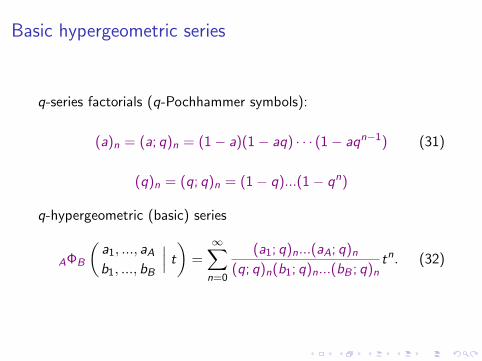
Basic hypergeometric series

q-series factorials (q-Pochhammer symbols):

(a)n = (a; q)n = (1− a)(1− aq) ⋅ ⋅ ⋅ (1− aqn−1) (31)

(q)n = (q; q)n = (1− q)...(1− qn)

q-hypergeometric (basic) series

AΦB

(a1, ..., aAb1, ..., bB

∣∣∣ t) =∞∑n=0

(a1; q)n...(aA; q)n(q; q)n(b1; q)n...(bB ; q)n

tn. (32)

Arithmetic of q-series

Amou M., Andre Y., Bertrand D., Bezivin, Borwein P., Bundschuh

P., Duverney D., Katsurada M., Merila V., Nesterenko Yu.,

Nishioka K., Prevost M., Rivoal T., Stihl Th., Shiokawa I.,

Waldscmidt M., Wallisser R., Vaananen K., Zudilin W.

q-world numbers

p-adic, p ∈ ℙ:∞∑n=1

pn

1− pn/∈ ℚ (33)

∞∑n=1

pn

n∏i=1

1± pi/∈ ℚ (34)

∞∑n=0

pn2∏n

j=1(1± pj)2/∈ ℚ (35)

q-world numbers

1 +p

1 +

p2

1 +

p3

1 + . . ./∈ ℚ (36)

∞∏n=1

(1 + kpn), k = 1, ..., p − 1, (37)

∞∑n=1

pnn∏

i=1

(1 + kpi ), k = 1, ..., p − 1, (38)

For the set (37) [Vaananen] gave

dimℚ = p (39)

True also for the set (38).

q-world numbers

Real, p ∈ ℤ ∖ {0,±1}:

∞∑n=1

1

1− pn/∈ ℚ (40)

∞∑n=1

1n∏

i=11± pi

/∈ ℚ (41)

∞∑n=0

1∏nj=1(1± pj)2

/∈ ℚ (42)

q-world numbers

1 +p−1

1 +

p−2

1 +

p−3

1 + . . ./∈ ℚ [Bundschuh] (43)

∞∏n=1

(1 + kp−n), k = 0, 1, ..., p − 1, (44)

∞∑n=1

p−nn∏

i=1

(1 + kp−i ), k = 0, 1, ..., p − 1. (45)

For the set (37) [Vaananen] gave

dimℚ = p (46)

True also for the set (38).

q-world numbers

∞∑n=0

1

Fan+b/∈ ℚ (47)

∞∑n=0

1

Lan+b/∈ ℚ (48)

where a, b,∈ ℤ+, Fn and Ln are the Fibonacci and Lucas numbers,

respectively; F0 = 0,F1 = 1, L0 = 2, L1 = 1.

[Andre-Jeannin]: a = 1; [Bundschuh+Vaananen] with a measure.

[Prevost+T.M.]: a, b ≥ 1 with irrationality measures; [Merila].

IRRATIONALITY MEASURE

By an effective irrationality measure (exponent) of a given number

� ∈ ℂp we mean a number � = �(�) ≥ 2 which satisfies the

condition: for every � > 0 there exists an effectively computable

constant H0(�) ≥ 1 such that∣∣∣∣� − M

N

∣∣∣∣p

>1

H�+�(49)

for every M/N ∈ ℚ with H = max{∣M∣, ∣N∣} ≥ H0(�).

Irrationality measures of explicit numbers

�(e) = 2 Classical (50)

�(log 2) ≤ 3.8914 [Rukhadze] (51)

�(log 3) ≤ 5.125 [Salikhov] (52)

�(�) ≤ 8.0161 [Hata] (53)

�(�(2)) ≤ 5.4413 [Rhin+Viola] (54)

�(�(3)) ≤ 5.5139 [Rhin+Viola] (55)

Irrationality measures of explicit numbers

�1 =1

F1 +

1

F2 +

1

F3 + . . ., �(�1) = 2 (56)

�2 =1

L1 +

1

L2 +

1

L3 + . . ., �(�2) = 2 (57)

∣∣∣∣�i − M

N

∣∣∣∣ ≥ C

N2+D/√logN

(58)

Linear forms

Let Θ ∈ ℂp be a number to be studied.

a) p =∞. I an imaginary quadratic field and ℤI ring of integers.

b) p ∈ ℙ = {2, 3, 5, ...}. I = ℚ.

Linear forms

In the following theorems put

Q(n) = ea(n), R(n) = e−b(n) (59)

where

a(n) = an, b(n) = bn (classical) (60)

or

a(n) = an log n, b(n) = bn log n (classical) (61)

and

a(n) = an2, b(n) = bn2 (q-world). (62)

Linear forms

Assume that

Rn = BnΘ− An ∀n ∈ ℕ (63)

are numerical approximation forms satisfying

Bn, An ∈ ℤI (64)

BnAn+1 − AnBn+1 ∕= 0, (65)

∣Bn∣ ≤ Q(n), and also (66)

∣An∣ ≤ Q(n), if p ∕=∞ (67)

∣Rn∣p ≤ R(n) (68)

for all n ≥ n0 with some positive a and b and a < b, if p ∕=∞.

Linear forms/Axiomatic

Let the above assumptions be valid. Then for every � > 0 there

exists a constant H0 = H0(�) ≥ 1 such that∣∣∣∣Θ− M

N

∣∣∣∣p

> H−�−� (69)

for all M,N ∈ ℤI with H ≥ H0, where (by folkflore)

� = 1 + a/b, H = ∣N∣, if p =∞, (70)

� =b

b − a, H = max{∣M∣, ∣N∣}, if p ∈ ℙ. (71)

Kalle Leppala (Master thesis): Axiomatic for more general a(n)

and b(n).

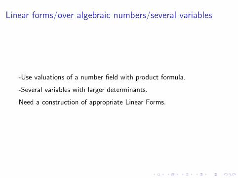
Linear forms/over algebraic numbers/several variables

-Use valuations of a number field with product formula.

-Several variables with larger determinants.

Need a construction of appropriate Linear Forms.

Pade approximations/Classical case

First we will study the classical series F (t) with it’s derivativies

ΔbF (t), where Δ = t ddt .

Denote d = max{degP(y), degQ(y)} and let d ,m ∈ ℤ+ and the

numbers �1, ..., �m be given.

We start by giving explicit type II Pade approximations for the

series

ΔbF (t�j), b = 0, 1, ..., d − 1; j = 1, ...,m. (72)

Our construction is based on a product expansion a la Maier

[Potenzreihen irrationalen Grenzwertes. J. Reine Angew. Math.

156, 93–148 (1927)]

Maier’s product formula

Let l ,m ∈ ℤ+ and � = t(�1, ..., �m) be given and define

�i = �i (l , �) bym∏t=1

(�t − w)l =ml∑i=0

�iwi . (73)

Thenml∑i=0

�i ik�i

t = 0 (74)

for all t ∈ {1, ...,m}; k ∈ {0, ..., l − 1}.

Maier’s product formula

Moreover

�i = (−1)i∑

i1+...+im=i

(l

i1

)⋅ ⋅ ⋅(

l

im

)⋅ �l−i1

1 ⋅ ⋅ ⋅�l−imm . (75)

Pade approximations/Classical case

Let b, d , l ,m, � ∈ ℕ, b < d and choose m numbers �1, ..., �m. Put

Bl ,�(t) =ml∑i=0

tml−i�i (l , �)[Q]i+�+⌊l/d⌋−1

[P]i+�. (76)

Then

Bl ,�(t)ΔbF (�j t)− Al ,�,b,j(t) = Rl ,�,b,j(t), (77)

where

degt Bl ,�(t) = ml , degt Al ,�,b,j(t) ≤ ml + �− 1 (78)

ordt=0

Rl ,�,b,j(t) ≥ ml + ⌊l/d⌋+ �. (79)

Pade approximations/Classical case

Thus we have a gap of lenght ⌊l/d⌋ in the power series expansion

Bl ,�(t)ΔbF (�j t) = Al ,�,b,j(t) + Rl ,�,b,j(t). (80)

The polynomials Bl ,�(t) are Pade approximant denominators in

variable t for the functions Fb,j(t) = ΔbF (t�j),

b = 0, 1, ..., d − 1; j = 1, ...,m.

Also we say that (77–79) define a Pade approximation with the

degree and order parameters

[degt B, degt A ≤, ordt=0

R ≥] = [ml ,ml + �− 1,ml + ⌊l/d⌋+ �]

(81)