Aachen Institute for Advanced Study in Computational Engineering Science

Preprint: AICES-2007-1

27/September/2007

A Corrected XFEM Approximation without Problems in

Blending Elements

T. P. Fries

Financial support from the Deutsche Forschungsgemeinschaft (German Research Association) through

grant GSC 111 is gratefully acknowledged.

©T. P. Fries 2007. All rights reserved

List of AICES technical reports: http://www.aices.rwth-aachen.de/preprints

A orre ted XFEM approximation without problemsin blending elementsThomas-Peter FriesSeptember 27, 2007Abstra tThe extended nite element method (XFEM) enables lo al enri hments of approx-imation spa es. Standard nite elements are used in the major part of the domainand enri hed elements are employed where spe ial solution properties su h as dis on-tinuities and singularities shall be aptured. In elements that blend the enri hed areaswith the rest of the domain problems arise in general. These blending elements oftenrequire a spe ial treatment in order to avoid a de rease in the overall onvergen erate. A modi ation of the XFEM-approximation is proposed in this work. Theenri hment fun tions are modied su h that they are zero in the standard elements,un hanged in the elements with all their nodes being enri hed, and varying ontinu-ously in the blending elements. All nodes in the blending elements are enri hed. Themodied enri hment fun tion an be reprodu ed exa tly everywhere in the domainand no problems arise in the blending elements. The orre ted XFEM is applied toproblems in linear elasti ity and optimal onvergen e rates are a hieved.Contents1 Introdu tion 32 General Formulation of the Standard and Corre ted XFEM 52.1 Standard XFEM . . . . . . . . . . . . . . . . . . . . . . . . . . . . . . . . 62.2 Blending Elements . . . . . . . . . . . . . . . . . . . . . . . . . . . . . . . 8

2 CONTENTS2.3 Corre ted XFEM . . . . . . . . . . . . . . . . . . . . . . . . . . . . . . . . 92.4 Shifted Enri hment Fun tions . . . . . . . . . . . . . . . . . . . . . . . . . 122.5 Several Enri hments . . . . . . . . . . . . . . . . . . . . . . . . . . . . . . 133 Spe ialization to Dis ontinuities 143.1 Des ription of Dis ontinuities . . . . . . . . . . . . . . . . . . . . . . . . . 143.2 Enri hment Fun tions . . . . . . . . . . . . . . . . . . . . . . . . . . . . . 153.2.1 Weak Dis ontinuities . . . . . . . . . . . . . . . . . . . . . . . . . . 153.2.2 Strong Dis ontinuities . . . . . . . . . . . . . . . . . . . . . . . . . 163.2.3 Cra k Tips . . . . . . . . . . . . . . . . . . . . . . . . . . . . . . . 173.3 Integration . . . . . . . . . . . . . . . . . . . . . . . . . . . . . . . . . . . . 184 Numeri al Results for Linear Elasti ity 204.1 Governing Equations . . . . . . . . . . . . . . . . . . . . . . . . . . . . . . 204.2 One-dimensional Bar: Pat h Test . . . . . . . . . . . . . . . . . . . . . . . 214.3 One-dimensional Bar: Convergen e Study . . . . . . . . . . . . . . . . . . 234.4 Two-dimensional Bi-material Problem . . . . . . . . . . . . . . . . . . . . . 254.5 Edge-Cra k Problem . . . . . . . . . . . . . . . . . . . . . . . . . . . . . . 304.5.1 Bran h-enri hment with Constant Radius . . . . . . . . . . . . . . . 324.5.2 Bran h-enri hment of the Cra k-tip Element Nodes . . . . . . . . . 345 Summary and Con lusions 37Referen es 40

31 Introdu tionA large number of models in ontinuum me hani s involve solutions that are non-smooth inlo al parts of the domain. There, state variables may exhibit dis ontinuities, singularities,or large gradients in general. For example, in solid me hani s, stresses and strains jumpalong material interfa es, displa ements hange dis ontinuously along ra ks, and strainsmay be singular at a ra k-tip. In uid me hani s, high gradients are present near sho ksand boundary layers.The nite element method (FEM) is highly suited for the approximation of smooth so-lutions [1, 2. It relies on the approximation properties of (mapped) polynomials [3, 4.Spe ial are has to be taken for approximating non-smooth solutions with the FEM. The onstru tion of an appropriate mesh is ru ial for the su ess of the approximation: Ele-ment edges have to align with a dis ontinuity and a mesh renement is required where thesolution is expe ted to have singularities or large gradients. Espe ially for the ase of mov-ing dis ontinuities, e.g. for the propagation of a ra k or for the movement of an interfa ebetween two uids, the maintenan e of an adequate mesh is di ult or even impossible.In ontrast, the extended nite element method (XFEM) [5, 6 oers the in lusion of apriori known solution properties into the approximation spa e. The simulation is often arried out on xed, simple (e.g. stru tured) meshes so that the mesh onstru tion andmaintenan e is redu ed to a minimum. The lo al enri hment of the approximation spa ein the XFEM is realized by means of the partition of unity on ept [4, 7. The enri hmentfun tions employed may enable the approximation to reprodu e kinks, jumps, singularitieset . exa tly in lo al parts of the domain. Referen es where the XFEM has been su essfullyemployed for dis ontinuities are found e.g. in [5, 8, 9, 10, and for dis ontinuous derivativesin [11, 12, 13, 14.Let us onsider the situation where a ertain enri hment fun tion is able to apture somenon-smooth solution hara teristi s in a lo al part of the domain. The nodes near thislo al subdomain are enri hed. Then, elements result in the overall domain with all, some,or none of their element nodes being enri hed. Elements with all nodes being enri hedare able to reprodu e the enri hment fun tion exa tly (reprodu ing elements). Elementswith no enri hed element nodes are standard nite elements; they are employed in thoseparts of the domain where the solution is smooth. Elements with some of their nodes beingenri hed are alled blending elements. They blend the enri hed subdomain with the restof the domain where only standard nite elements are employed.

4 Introdu tionBlending elements in the XFEM show, in general, two important properties: (i) In theseelements, the enri hment fun tion an no longer be reprodu ed exa tly (be ause of a la k ofa partition of unity). (ii) These elements produ e unwanted terms into the approximationwhi h annot be ompensated by the standard nite element part of the approximation.For example, a linear fun tion an no longer be represented in a linear blending elementif the enri hment introdu es non-linear terms. The rst aspe t does not pose a signi antproblem in the XFEM, however, the se ond one may signi antly redu e the onvergen erate for general enri hment fun tions [15, 16. Suboptimal onvergen e rates due to prob-lems in blending elements have been found in [16, 17, 18.A spe ial treatment is in general required in blending elements in order to get rid of theunwanted terms. Among the existing approa hes are those whi h use enhan ed strainte hniques or p-renement in blending elements [15. Another approa h whi h adjusts theorder of the nite element shape fun tions depending on the enri hment is dis ussed e.g. in[19. Modi ations of the standard XFEM approximation in order to ir umvent problemsin blending elements for the ase of ra k appli ations are dis ussed in [16. It is noted thatfor the parti ular ase of the sign- and Heaviside-enri hment, no problems in blending ele-ments result. For solutions that involve a kink along an interfa e, this enri hment is often hosen although additional onstraints are needed to ensure the ontinuity, e.g. [20, 21.This may also be onsidered a spe ial te hnique to avoid problems in blending elements be- ause other enri hments are more appropriate, i.e. they do not need additional onstraints,but introdu e problems in blending elements. All these approa hes share the propertythat they are not easily extended to arbitrary enri hment fun tions, element types, andmathemati al models.In this work, a modied denition of the XFEM approximation is proposed. Throughoutthis paper this is referred to as modied XFEM or orre ted XFEM, whereas the orig-inal denition is alled standard XFEM. Two important dieren es an be found in theapproximations of the standard and orre ted XFEM: (i) In addition to those nodes thatare enri hed in the standard XFEM, all nodes in the blending elements are enri hed. Thatis, a omplete partition of unity is present in the reprodu ing and blending elements. (ii)The enri hment fun tions of the standard XFEM are modied ex ept in the reprodu ingelements. They are zero in the standard nite elements, and in the blending elements,they vary ontinuously between the standard and reprodu ing elements. The modi ationof the enri hment fun tion is realized by means of a ramp fun tion.The orre ted XFEM is able to reprodu e the modied enri hment fun tion exa tly ev-

5erywhere in the domain. The original enri hment fun tion an be found exa tly in thereprodu ing elements. Most importantly, there are no unwanted terms in the blendingelements. Therefore, the orre ted XFEM is able to a hieve optimal onvergen e wherethe standard XFEM only a hieves redu ed onvergen e rates due to problems in the blend-ing elements. The modied approximation of the proposed XFEM version an be appliedfor general enri hment fun tions, element types and mathemati al models. The modiedXFEM ts into the general framework of the standard XFEM and is, therefore, easy toimplement in existing XFEM odes. The total number of degrees of freedom is slightlyin reased ompared to the standard XFEM. The numeri al results prove the su ess of themodied XFEM.The paper is organized as follows: Se tion 2 des ribes the standard and orre ted XFEMon a general level suited for arbitrary enri hment fun tions. The approximation of thestandard XFEM is given in se tion 2.1, followed by a dis ussion of blending elements andthe resulting problems in the standard XFEM. Se tion 2.3 denes the modied approxima-tion proposed in this work. In the XFEM, it is often useful to shift enri hment fun tionssu h that the Krone ker-δ property of the approximation is maintained, this is shown inse tion 2.4 for the standard and modied XFEM. The generalization to more than one en-ri hment fun tion is given in se tion 2.5. The spe ialization of the general approximationsto the parti ular ase of dis ontinuities is dis ussed in se tion 3. It starts with a shortreview of the levelset method for the des ription of dis ontinuities. Se tion 3.2 denesparti ular enri hment fun tions and the resulting approximations in the modied XFEMfor strong and weak dis ontinuities and ra k-tips. Numeri al results are given in se tion4 for problems in linear elasti ity. Optimal onvergen e is a hieved for a bi-material test ase and ra k appli ations. The results are signi antly better than those obtained bythe standard XFEM.2 General Formulation of the Standard and Corre tedXFEMIn this se tion, the standard and proposed modied XFEM are dis ussed in a general way.All appli ations of the XFEM an be based on the general form of the approximationshown in this se tion. An XFEM approximation onsists of a standard nite element partand the enri hments. The enri hment terms are onstru ted by means of partition of unity

6 General Formulation of the Standard and Corre ted XFEMfun tions and enri hment fun tions that enable the approximation to apture spe ial non-polynomial solution hara teristi s in lo al parts of the domain. A spe ialization of thegeneral XFEM approximations to on rete appli ations su h as dis ontinuities is dis ussedin the next se tion.2.1 Standard XFEMConsider an n-dimensional domain Ω ∈ Rn whi h is dis retized by nel elements, numberedfrom 1 to nel. I is the set of all nodes in the domain, and Iel

k are the element nodes ofelement k ∈1, . . . , nel

. A standard extended nite element approximation of a fun tionu (x) is of the form

uh (x) =∑

i∈I

Ni (x) ui

︸ ︷︷ ︸

+∑

i∈I⋆

Mi (x) ai

︸ ︷︷ ︸

,strd. FE approx. enri hment (2.1)where for simpli ity only one enri hment term is onsidered. The approximation onsistsof a standard nite element (FE) part and the enri hment. The individual variables standforuh (x) : approximated fun tion,Ni (x) : standard FE fun tion of node i,

ui : unknown of the standard FE part at node i,I : set of all nodes in the domain,

Mi (x) : lo al enri hment fun tion of node i,ai : unknown of the enri hment at node i,I⋆ : nodal subset of the enri hment, I⋆ ⊂ I.The enri hment is built by lo al enri hment fun tions Mi (x) and unknowns ai whi h aredened at nodes in I⋆ ⊂ I. The lo al enri hment fun tions have the form

Mi (x) = N⋆i (x) · ψ (x) , ∀i ∈ I⋆, (2.2)and we all N⋆

i (x) partition of unity fun tions and ψ (x) global enri hment fun tion. The

2.1 Standard XFEM 7fun tions N⋆i (x) are standard FE shape fun tions whi h are not ne essarily the same thanthose of the standard part of the approximation (2.1). These fun tions build a partitionof unity,

∑

i∈I⋆

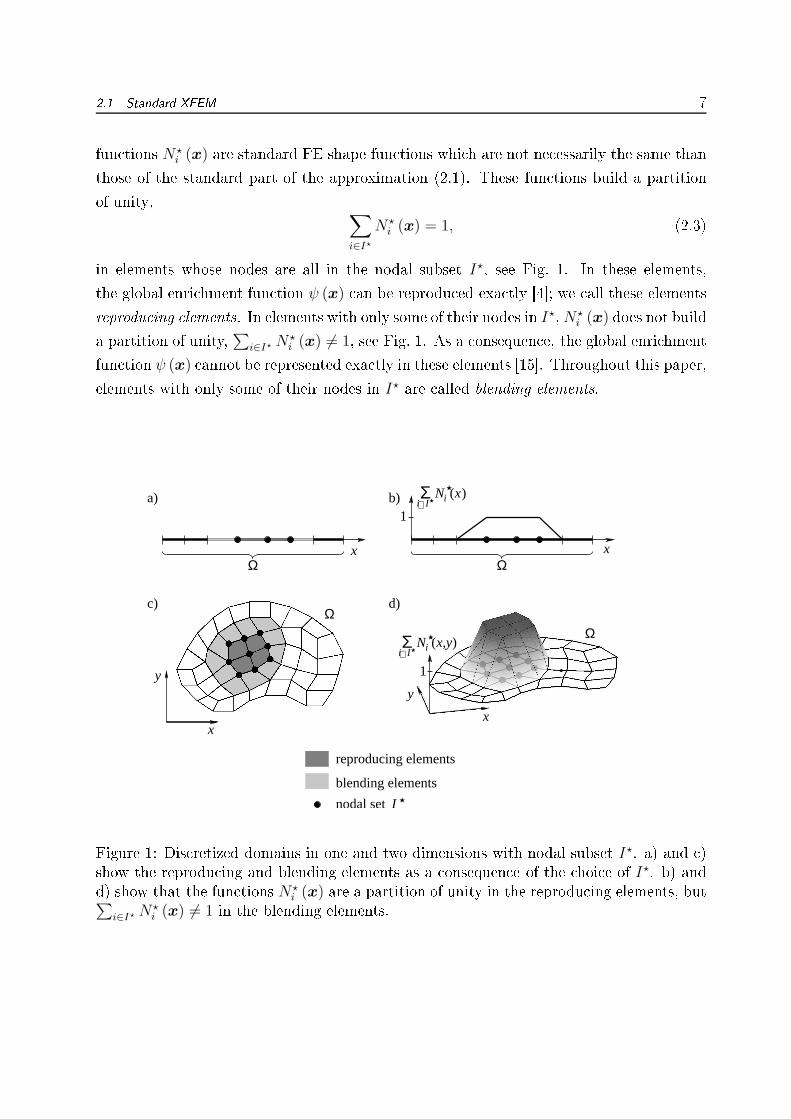
N⋆i (x) = 1, (2.3)in elements whose nodes are all in the nodal subset I⋆, see Fig. 1. In these elements,the global enri hment fun tion ψ (x) an be reprodu ed exa tly [4; we all these elementsreprodu ing elements. In elements with only some of their nodes in I⋆, N⋆

i (x) does not builda partition of unity, ∑

i∈I⋆ N⋆i (x) 6= 1, see Fig. 1. As a onsequen e, the global enri hmentfun tion ψ (x) annot be represented exa tly in these elements [15. Throughout this paper,elements with only some of their nodes in I⋆ are alled blending elements.

x

i ∋I (xNi

Σ )

i ∋I (x,y)Ni

Σ

Ω Ω

blending elements

reproducing elements

nodal setI

x

y

1y

xx

1

ΩΩ

b)a)

c) d)

Figure 1: Dis retized domains in one and two dimensions with nodal subset I⋆. a) and )show the reprodu ing and blending elements as a onsequen e of the hoi e of I⋆. b) andd) show that the fun tions N⋆i (x) are a partition of unity in the reprodu ing elements, but

∑

i∈I⋆ N⋆i (x) 6= 1 in the blending elements.

8 General Formulation of the Standard and Corre ted XFEM2.2 Blending ElementsLet us onsider the situation in the blending elements of the standard XFEM more losely.In these elements, ∑

i∈I⋆ N⋆i (x) 6= 1, i.e. the fun tions N⋆

i (x) are not a partition of unity.As a onsequen e, the approximation is no longer able to represent the enri hment fun tionψ (x) exa tly. This fa t, however, does not pose a severe problem be ause one is interestedin apturing lo al phenomena through the enri hment. Through the hoi e of the nodalsubset I⋆ one an dire tly pres ribe the lo al area of the domain where the enri hmentfun tion an be represented exa tly be ause the fun tions N⋆

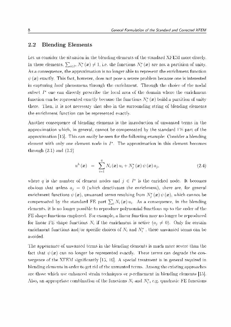
i (x) build a partition of unitythere. Then, it is not ne essary that also in the surrounding string of blending elementsthe enri hment fun tion an be represented exa tly.Another onsequen e of blending elements is the introdu tion of unwanted terms in theapproximation whi h, in general, annot be ompensated by the standard FE part of theapproximation [15. This an easily be seen for the following example: Consider a blendingelement with only one element node in I⋆. The approximation in this element be omesthrough (2.1) and (2.2)uh (x) =

q∑

i=1

Ni (x) ui +N⋆j (x)ψ (x) aj , (2.4)where q is the number of element nodes and j ∈ I⋆ is the enri hed node. It be omesobvious that unless aj = 0 (whi h dea tivates the enri hment), there are, for generalenri hment fun tions ψ (x), unwanted terms resulting from N⋆

j (x)ψ (x), whi h annot be ompensated by the standard FE part ∑

iNi (x) ui. As a onsequen e, in the blendingelements, it is no longer possible to reprodu e polynomial fun tions up to the order of theFE shape fun tions employed. For example, a linear fun tion may no longer be reprodu edfor linear FE shape fun tions Ni if the enri hment is a tive (aj 6= 0). Only for ertainenri hment fun tions and/or spe i hoi es of Ni and N⋆i , these unwanted terms an beavoided.The appearan e of unwanted terms in the blending elements is mu h more severe than thefa t that ψ (x) an no longer be represented exa tly. These terms an degrade the on-vergen e of the XFEM signi antly [15, 16. A spe ial treatment is in general required inblending elements in order to get rid of the unwanted terms. Among the existing approa hesare those whi h use enhan ed strain te hniques or p-renement in blending elements [15.Also, an appropriate ombination of the fun tions Ni and N⋆

i , e.g. quadrati FE fun tions

2.3 Corre ted XFEM 9for Ni and linear FE fun tions for N⋆i , may improve the situation for ertain (e.g. polyno-mial) enri hment fun tions ψ [19. Most of these approa hes share the property that theyhave to be designed or at least adjusted for ea h enri hment fun tion ψ individually.It is added for ompleteness that it is not possible to simply set N⋆

i (x) to zero in theblending elements. Then, the approximation would not introdu e unwanted terms in theblending elements and would still be able to represent the enri hment fun tion exa tly inthe reprodu ing elements. However, the resulting lo al enri hment fun tions Mi (x) wouldbe dis ontinuous along the element edges between the reprodu ing and blending elements.2.3 Corre ted XFEMA modied formulation of the XFEM-approximation is proposed in this se tion. Thismodi ation avoids unwanted terms in the blending elements and still leads to ontinuouslo al enri hment fun tions (as long as ψ is ontinuous).Let us dene a modied enri hment fun tion ψmod (x) asψmod (x) = ψ (x) · R (x) , (2.5)with R (x) being a ramp fun tion

R (x) =∑

i∈I⋆

N⋆i (x) . (2.6)A graphi al representation of R (x) may be seen in Fig. 1(b) and (d) for one- and two-dimensional domains. It is obvious that ψmod (x) = ψ (x) in the reprodu ing elements(all element nodes are in I⋆). Furthermore, ψmod (x) = 0 in standard nite elements (noelement nodes are in I⋆). In the blending elements (some element nodes are in I⋆), themodied enri hment fun tion ψmod (x) varies ontinuously between ψ (x) and zero. There,due to the multipli ation with R (x), the order of ψmod (x) is in reased when ompared to

ψ (x), and slightly more integration points may be appropriate for the integration.A nodal subset J⋆ ⊂ I is introdu ed whi h onsists of all element nodes of the reprodu ingand blending elements. In other words, J⋆ is the set of nodes in I⋆ plus their neighboringnodes (those nodes that share elements with nodes in I⋆). Clearly, I⋆ ⊂ J⋆, whi h an also

10 General Formulation of the Standard and Corre ted XFEMΩ

a)Ω

b)

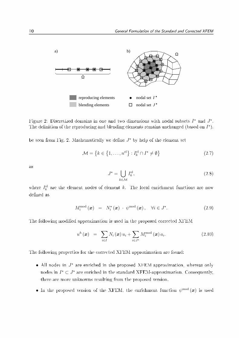
nodal setJblending elements

reproducing elements nodal setI

Figure 2: Dis retized domains in one and two dimensions with nodal subsets I⋆ and J⋆.The denition of the reprodu ing and blending elements remains un hanged (based on I⋆).be seen from Fig. 2. Mathemati ally we dene J⋆ by help of the element setM =

k ∈

1, . . . , nel

: Iel

k ∩ I⋆ 6= ∅ (2.7)as

J⋆ =⋃

k∈M

Ielk , (2.8)where Iel

k are the element nodes of element k. The lo al enri hment fun tions are nowdened asMmod

i (x) = N⋆i (x) · ψmod (x) , ∀i ∈ J⋆. (2.9)The following modied approximation is used in the proposed orre ted XFEM

uh (x) =∑

i∈I

Ni (x) ui +∑

i∈J⋆

Mmodi (x) ai. (2.10)The following properties for the orre ted XFEM approximation are found:

• All nodes in J⋆ are enri hed in the proposed XFEM-approximation, whereas onlynodes in I⋆ ⊂ J⋆ are enri hed in the standard XFEM-approximation. Consequently,there are more unknowns resulting from the proposed version.• In the proposed version of the XFEM, the enri hment fun tion ψmod (x) is used

2.3 Corre ted XFEM 11instead of ψ (x).• The modied enri hment fun tion ψmod (x) is non-zero only in the reprodu ing andblending elements. Most importantly, it is zero in elements with only some of theirnodes in J⋆. That is, no unwanted terms are introdu ed by the proposed XFEM-approximation, and therefore, no need for any spe ial treatment in the blendingelements. In ontrast, in the standard XFEM-approximation, the enri hment fun -tion ψ (x) is non-zero in elements with only some of their nodes in I⋆, whi h leadsto the problem of unwanted terms as dis ussed in se tion 2.2.• In the proposed XFEM-approximation, N⋆

i (x) is a partition of unity in the reprodu -ing and blending elements. Consequently, the modied enri hment fun tion ψmod (x) an be reprodu ed exa tly in all elements where this fun tion is non-zero. In the stan-dard XFEM, however, the enri hment fun tion ψ (x) an only be reprodu ed exa tlyin the reprodu ing elements but not in the blending elements.It is noted that the denition of the reprodu ing and blending elements remains un hangedfor the modied XFEM, i.e. based on I⋆. We believe that this naming is still appropriatebe ause• it is still only possible to reprodu e ψ (x) exa tly in the reprodu ing elements. Onlyψmod (x) an also be reprodu ed exa tly in the blending elements.

• the blending elements still serve the purpose to blend the approximation in the en-ri hed part with the pure standard FE part. The dieren e in the orre ted XFEM isthat this is a hieved through ψmod (x) and the enri hment of all nodes of the blend-ing elements, opposed to using ψ (x) and enri hing only some nodes of the blendingelements as it is done in the standard XFEM.Remark (Hierar hi al blending elements) Hierar hi al blending elements with theaim to ompensate unwanted terms in the blending elements by in reasing the polynomialorder of the approximation in the blending elements are introdu ed in [15. A similaritywith the approa h proposed in this work is the employment of additional nodes in theblending elements. However, the hierar hi al blending elements are designed for polyno-mial enri hment fun tions (see [15, page 1026), whereas the modi ation proposed here isfor general enri hment fun tions. The pla ement of the additional nodes in the blending

12 General Formulation of the Standard and Corre ted XFEMelements and the denition of their shape fun tions dier in the two approa hes: In hi-erar hi al blending elements, nodes and shape fun tions are introdu ed based on lassi alhigher-order nite elements, whereas in this approa h, only the existing nodes of the blend-ing elements are used and their shape fun tions result through (2.9). It is also pointed outthat the two approa hes have dierent motivations: In hierar hi al blending elements, onetries to de rease the negative ee ts of the unwanted terms by in reasing the polynomialorder in the element. This alleviates the problems of unwanted terms in blending elementsbutespe ially for non-polynomial enri hment fun tionsdoes not fully ompensate them.In ontrast, the orre ted XFEM avoids unwanted terms from the beginning.2.4 Shifted Enri hment Fun tionsIn general, standard FE shape fun tions have the Krone ker-δ property, i.e. Ni (xj) = δij .In a standard FE approximation, uh (x) =∑

iNi (x)ui, this leads to the desirable featuresthat• the omputed unknowns ui are dire tly the sought fun tion values of uh (x) at nodei, i.e. uh (xi) = ui.

• the imposition of Diri hlet boundary onditions u (x) is simple: ui = u (xi).In standard XFEM approximations, see (2.1), these properties only hold for lo al enri h-ment fun tions that are zero at all nodes, i.e. Mi (xj) = 0, ∀i ∈ I⋆, ∀j ∈ I. This an bea hieved by shifting the global enri hment fun tion ψ (x) asψshift

i (x) = ψ (x) − ψ (xi) , ∀i ∈ I⋆,and using ψshifti (x) instead of ψ (x) in (2.2).For the proposed modied XFEM approximation, shifted enri hment fun tions with

Mmodi (xj) = 0, ∀i ∈ J⋆, ∀j ∈ I (2.11)are a hieved by setting

ψmod,shifti (x) = [ψ (x) − ψ (xi)] · R (x) , (2.12)

2.5 Several Enri hments 13with R (x) dened in (2.6). These shifted global enri hment fun tions are then used forthe denition of Mmodi asMmod

i (x) = N⋆i (x) · ψmod,shift

i (x) , ∀i ∈ J⋆. (2.13)It is easy to show that (2.11) holds for this denition: For i 6= j, N⋆i (xj) = 0 be ause theseare standard FE shape fun tions with the Krone ker-δ property. As a result, Mmod

i (xj) =

0. For i = j, ψ (xj) − ψ (xi) = 0, onsequently ψmod,shifti (xj) = 0 and Mmod

i (xj) = 0.2.5 Several Enri hmentsFor simpli ity, in the previous subse tions, only one enri hment term has been onsideredin the XFEM-approximations, see (2.1) and (2.10). The extension to several enri hmentsis straightforward. The approximations for m enri hments are of the form

uh (x) =∑

i∈I

Ni (x)ui +

m∑

j=1

∑

i∈I⋆j

M ji (x) aj

ifor the standard XFEM anduh (x) =

∑

i∈I

Ni (x) ui +m∑

j=1

∑

i∈J⋆j

M j,modi (x) aj

ifor the proposed modied XFEM. The denitions of the nodal subsets (I⋆j and J⋆

j ) andlo al enri hment fun tions (M ji and M j,mod

i ) are analogously to the previous subse tionsfor ea h of the m enri hment terms. A shifted, standard XFEM-approximation for severalenri hments be omesuh (x) =

∑

i∈I

Ni (x)ui +m∑

j=1

∑

i∈I⋆j

N⋆i (x) ·

[ψj (x) − ψj (xi)

]· aj

i . (2.14)In ontrast, the shifted, modied XFEM-approximation for several enri hments isuh (x) =

∑

i∈I

Ni (x) ui +m∑

j=1

∑

i∈J⋆j

N⋆i (x) ·

[ψj (x) − ψj (xi)

]· Rj (x) · aj

i . (2.15)

14 Spe ialization to Dis ontinuitiesIt is noted, that also for the modied XFEM-approximation, the nodal subsets I⋆j areneeded for the denition of the subsets J⋆

j , see (2.7) and (2.8), and the ramp fun tionsRj (x) =

∑

i∈I⋆j

N⋆i (x) .

3 Spe ialization to Dis ontinuitiesIn the previous se tion, the standard and modied XFEM are des ribed on a general levelwithout spe ifying the hoi e of the enri hed nodes and the enri hment fun tions. In pra -ti e, the XFEM is most often used for appli ations with dis ontinuities and singularitiesfor example near material interfa es, ra ks, ra k-tips, shear bands et . In this se tion,the des ription of dis ontinuities by means of the levelset method is briey mentioned.Some parti ularly useful enri hment fun tions, frequently used for strong and weak dis on-tinuities and near ra k-tips, are re alled together with a suitable hoi e of the enri hednodes. Throughout this paper, the partition of unity fun tions N⋆i are hosen identi al tothe shape fun tions of the standard FE part of the approximation, Ni.3.1 Des ription of Dis ontinuitiesThe levelset method [22 is used for the des ription of the dis ontinuities in the domain.It is a numeri al te hnique for the impli it tra king of moving interfa es and is frequentlyused in the ontext of the XFEM, see e.g. [17, 23, 24. The basi idea is outlined as follows:A domain Ω an be de omposed into two subdomains ΩA and ΩB by means of a s alarfun tion φ (x) : R

n → R whi h is positive in ΩA, negative in ΩB and zero on the interfa eΓdisc. In this work, the signed distan e fun tion [22 is used as a parti ular levelset fun tion,

φ (x) = ±min ‖x − xdisc‖ , ∀xdisc ∈ Γdisc, ∀x ∈ Ω, (3.1)where the sign is dierent on the two sides of the dis ontinuity and ‖ · ‖ denotes theEu lidean norm.Typi ally, the values of the levelset fun tion are only stored at nodes φi = φ (xi), and the

3.2 Enri hment Fun tions 15levelset fun tion is interpolated byφh (x) =

∑

i∈I

Ni (x)φi (3.2)using standard FE shape fun tions Ni as interpolation fun tions. The parti ular hoi eof these fun tions is worked out in se tion 3.3. It is noted that the representation of thedis ontinuity as the zero-level of φh (x) is only an approximation of the real position, whi himproves with mesh renement.Remark (Levelset method for ra ks) The dis ontinuity des ribed by one levelsetfun tion φ (x) is losed, i.e. there are no end points within the domain Ω. For the aseof ra ks, the dis ontinuity ends at the ra k-tip within the domain. Then, the ra k path an be stored in one levelset fun tion φ (x), and a se ond levelset fun tion ξ (x) an beused in order to dene the position of the ra k tip [23, 24, see Fig. 6.3.2 Enri hment Fun tions3.2.1 Weak Dis ontinuitiesA fun tion has a kink along weak dis ontinuities, i.e. it is ontinuous but with a dis ontin-uous gradient. The abs-enri hmentψ (x) = abs

(φh (x)

) (3.3)is frequently used for apturing weak dis ontinuities, see e.g. [11, 12, 13, 14, 17. Theenri hment term in the standard XFEM results as∑

i∈I⋆abs

N⋆i (x) ·

[abs

(φh (x)

)− abs

(φh (xi)

)]· ai, (3.4)The nodal subset I⋆

abs ontains all element nodes of elements ut by the dis ontinuity, seeFig. 3(a). The set of ut elements isN =

k ∈1, . . . , nel

: min

i∈Ielk

(φh (xi)

)· max

i∈Ielk

(φh (xi)

)< 0

, (3.5)

16 Spe ialization to Dis ontinuitieswhere Ielk are the element nodes of element k. Then, I⋆

abs follows asI⋆abs =

⋃

k∈N

Ielk . (3.6)The enri hment term of the modied XFEM is

∑

i∈J⋆abs

N⋆i (x) ·

[abs

(φh (x)

)− abs

(φh (xi)

)]· Rabs (x) · ai, (3.7)where the nodal set J⋆

abs and the ramp fun tion Rabs (x) are dened through Eqs. (2.6),(2.7), and (2.8) by means of the nodal set I⋆ = I⋆abs.

3.2.2 Strong Dis ontinuitiesA fun tion shows a jump along strong dis ontinuities. Typi ally, the sign-enri hment isused in this ase, see e.g. [5, 8, 9, 10,ψ (x) = sign

(φh (x)

). (3.8)It is important to note that the sign-enri hment is a spe ial ase, where also the standardXFEM does not lead to problems in blending elements. The reason is that the sign-enri hment is a onstant fun tion in the blending elements and as long as the partition ofunity fun tions N⋆

i are of the same or lower order than the shape fun tions of the standardFE part Ni, the unwanted terms in the blending elements an be ompensated. For the ase of the shifted sign-enri hment, the enri hment fun tions Mi in the blending elementsredu e to zero whi h immediately shows that no unwanted terms an o ur.Therefore, for the spe ial ase of the sign-enri hment, there is no need for a modi ationof the standard XFEM and the enri hment for standard and modied XFEM is∑

i∈I⋆sign

N⋆i (x) ·

[sign

(φh (x)

)− sign

(φh (xi)

)]· ai. (3.9)The nodal set I⋆

sign is hosen in the same way than for weak dis ontinuities, see (3.6),i.e. I⋆sign = I⋆

abs.

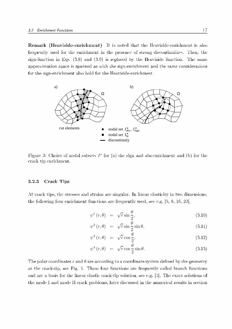
3.2 Enri hment Fun tions 17Remark (Heaviside-enri hment) It is noted that the Heaviside-enri hment is alsofrequently used for the enri hment in the presen e of strong dis ontinuities. Then, thesign-fun tion in Eqs. (3.8) and (3.9) is repla ed by the Heaviside fun tion. The sameapproximation spa e is spanned as with the sign-enri hment and the same onsiderationsfor the sign-enri hment also hold for the Heaviside-enri hment.absI signI

brI

discontinuity

nodal set ,nodal set

Ω

r

b)

cut elements

Ω

a)

Figure 3: Choi e of nodal subsets I⋆ for (a) the sign and abs-enri hment and (b) for the ra k tip enri hment.3.2.3 Cra k TipsAt ra k tips, the stresses and strains are singular. In linear elasti ity in two dimensions,the following four enri hment fun tions are frequently used, see e.g. [5, 8, 16, 23,ψ1 (r, θ) =

√r sin

θ

2, (3.10)

ψ2 (r, θ) =√r sin

θ

2sin θ, (3.11)

ψ3 (r, θ) =√r cos

θ

2, (3.12)

ψ4 (r, θ) =√r cos

θ

2sin θ. (3.13)The polar oordinates r and θ are a ording to a oordinate system dened by the geometryat the ra k-tip, see Fig. 4. These four fun tions are frequently alled bran h fun tionsand are a basis for the linear elasti ra k-tip solution, see e.g. [5. The exa t solutions ofthe mode I and mode II ra k problems, later dis ussed in the numeri al results in se tion

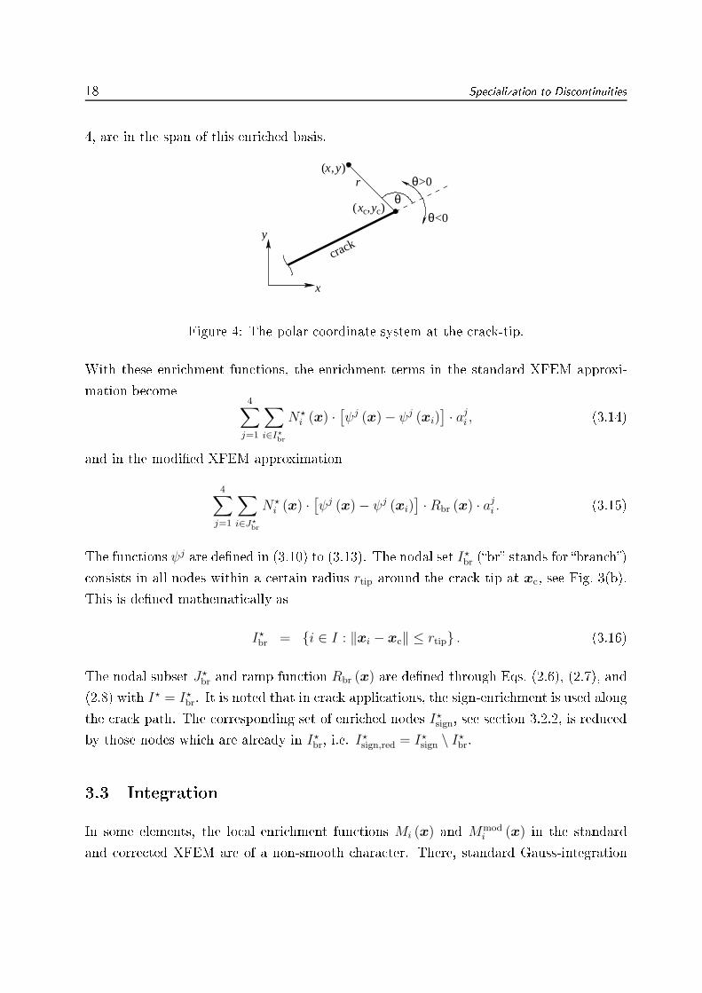
18 Spe ialization to Dis ontinuities4, are in the span of this enri hed basis.θ<0

θ>0

y

x

c(x c,y )

r

θ

)yx( ,

crack

Figure 4: The polar oordinate system at the ra k-tip.With these enri hment fun tions, the enri hment terms in the standard XFEM approxi-mation be ome4∑

j=1

∑

i∈I⋆br

N⋆i (x) ·

[ψj (x) − ψj (xi)

]· aj

i , (3.14)and in the modied XFEM approximation4∑

j=1

∑

i∈J⋆br

N⋆i (x) ·

[ψj (x) − ψj (xi)

]· Rbr (x) · aj

i . (3.15)The fun tions ψj are dened in (3.10) to (3.13). The nodal set I⋆br (br stands for bran h) onsists in all nodes within a ertain radius rtip around the ra k tip at xc, see Fig. 3(b).This is dened mathemati ally as

I⋆br = i ∈ I : ‖xi − xc‖ ≤ rtip . (3.16)The nodal subset J⋆

br and ramp fun tion Rbr (x) are dened through Eqs. (2.6), (2.7), and(2.8) with I⋆ = I⋆br. It is noted that in ra k appli ations, the sign-enri hment is used alongthe ra k path. The orresponding set of enri hed nodes I⋆

sign, see se tion 3.2.2, is redu edby those nodes whi h are already in I⋆br, i.e. I⋆

sign,red = I⋆sign \ I⋆

br.3.3 IntegrationIn some elements, the lo al enri hment fun tions Mi (x) and Mmodi (x) in the standardand orre ted XFEM are of a non-smooth hara ter. There, standard Gauss-integration

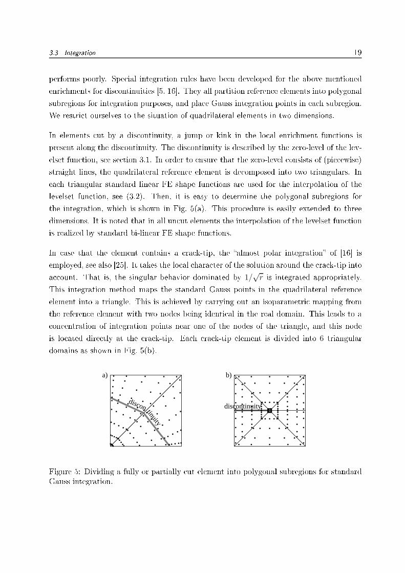
3.3 Integration 19performs poorly. Spe ial integration rules have been developed for the above mentionedenri hments for dis ontinuities [5, 16. They all partition referen e elements into polygonalsubregions for integration purposes, and pla e Gauss integration points in ea h subregion.We restri t ourselves to the situation of quadrilateral elements in two dimensions.In elements ut by a dis ontinuity, a jump or kink in the lo al enri hment fun tions ispresent along the dis ontinuity. The dis ontinuity is des ribed by the zero-level of the lev-elset fun tion, see se tion 3.1. In order to ensure that the zero-level onsists of (pie ewise)straight lines, the quadrilateral referen e element is de omposed into two triangulars. Inea h triangular standard linear FE shape fun tions are used for the interpolation of thelevelset fun tion, see (3.2). Then, it is easy to determine the polygonal subregions forthe integration, whi h is shown in Fig. 5(a). This pro edure is easily extended to threedimensions. It is noted that in all un ut elements the interpolation of the levelset fun tionis realized by standard bi-linear FE shape fun tions.In ase that the element ontains a ra k-tip, the almost polar integration of [16 isemployed, see also [25. It takes the lo al hara ter of the solution around the ra k-tip intoa ount. That is, the singular behavior dominated by 1/√r is integrated appropriately.This integration method maps the standard Gauss points in the quadrilateral referen eelement into a triangle. This is a hieved by arrying out an isoparametri mapping fromthe referen e element with two nodes being identi al in the real domain. This leads to a on entration of integration points near one of the nodes of the triangle, and this nodeis lo ated dire tly at the ra k-tip. Ea h ra k-tip element is divided into 6 triangulardomains as shown in Fig. 5(b).

b)a)

tinuity

discon discontinuity

Figure 5: Dividing a fully or partially ut element into polygonal subregions for standardGauss integration.

20 Numeri al Results for Linear Elasti ity4 Numeri al Results for Linear Elasti ity4.1 Governing EquationsA two-dimensional domain Ω with boundary Γ is onsidered. The boundary Γ is de om-posed into the omplementary sets Γu and Γt. Displa ements u are pres ribed along theDiri hlet boundary Γu, and tra tions t along the Neumann boundary Γt. Two dierentsituations are onsidered. In the rst ase, the domain falls into two subdomains withdierent material properties, separated by an interfa e Γdisc. Γdisc is a losed dis ontinu-ity, i.e. it does not end within the domain, see Fig. 6(a). In the se ond ase, the domainis ut partially by a ra k Γc. The one-dimensional ra k surfa e Γc is assumed to betra tion-free. See Fig. 6(b) for a sket h of the situation.The strong form for an elasti solid in two dimensions, undergoing small displa ements andstrains under stati onditions, is [1, 2∇ · σ = f , on Ω ⊆ R

2, (4.1)where f des ribe volume for es, and σ is the following stress tensorσ = C : ε = λ (tr ε) I + 2µε, (4.2)with λ and µ being the Lamé onstants. The linearized strain tensor ε is

ε =1

2

(

∇u + (∇u)T)

. (4.3)For the approximation of the displa ements u, the following test and trial fun tion spa esSh

uand Vh

uare introdu ed as

Shu

=

uh∣∣ uh ∈

(H1h

)d, uh = uh on Γu, uh dis . on Γc

, (4.4)Vh

u=

wh∣∣ wh ∈

(H1h

)d, wh = 0 on Γu, wh dis . on Γc

, (4.5)where H1h ⊆ H1 is a nite dimensional Hilbert spa e onsisting of the shape fun tions.The spa e H1 is the set of fun tions whi h are, together with their rst derivatives, square-integrable in Ω. The dis retized weak form may be formulated in the following Bubnov-

4.2 One-dimensional Bar: Pat h Test 21Galerkin setting [1, 2: Find uh ∈ Shusu h that

∫

Ω

σ(uh

): ε

(wh

)dΩ =

∫

Ω

wh · fhdΩ +

∫

Γt

wh · thdΓ ∀wh ∈ Vh

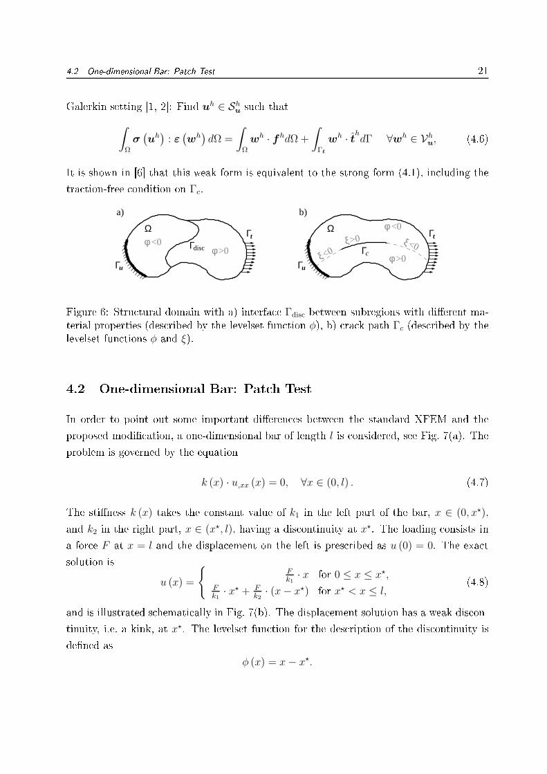
u, (4.6)It is shown in [6 that this weak form is equivalent to the strong form (4.1), in luding thetra tion-free ondition on Γc.

Γu

Γt

Γdisc

Γu

ξ<0Γt

ξ<0 Γc

Ω

a)

Ω

b)

ξ>0<0φ>0φ

<0φ

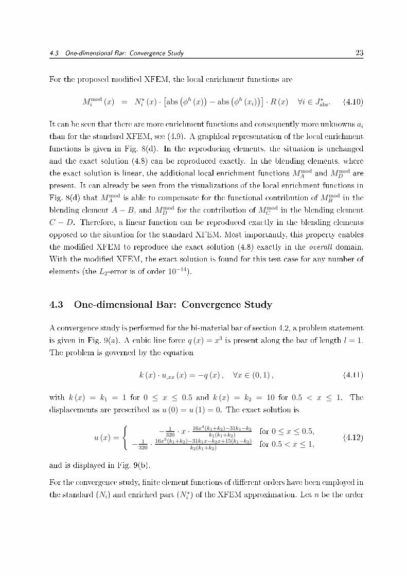
>0φFigure 6: Stru tural domain with a) interfa e Γdisc between subregions with dierent ma-terial properties (des ribed by the levelset fun tion φ), b) ra k path Γc (des ribed by thelevelset fun tions φ and ξ).4.2 One-dimensional Bar: Pat h TestIn order to point out some important dieren es between the standard XFEM and theproposed modi ation, a one-dimensional bar of length l is onsidered, see Fig. 7(a). Theproblem is governed by the equationk (x) · u,xx (x) = 0, ∀x ∈ (0, l) . (4.7)The stiness k (x) takes the onstant value of k1 in the left part of the bar, x ∈ (0, x⋆),and k2 in the right part, x ∈ (x⋆, l), having a dis ontinuity at x⋆. The loading onsists ina for e F at x = l and the displa ement on the left is pres ribed as u (0) = 0. The exa tsolution is

u (x) =

Fk1

· x for 0 ≤ x ≤ x⋆,Fk1

· x⋆ + Fk2

· (x− x⋆) for x⋆ < x ≤ l,(4.8)and is illustrated s hemati ally in Fig. 7(b). The displa ement solution has a weak dis on-tinuity, i.e. a kink, at x⋆. The levelset fun tion for the des ription of the dis ontinuity isdened as

φ (x) = x− x⋆.

22 Numeri al Results for Linear Elasti ityF/k1

F/k21

1x

k1 k2 F

A B C

bar

lx0

u

b)

a)

DFigure 7: a) Problem statement for the one-dimensional bi-material bar with the nodenumbering near the dis ontinuity, b) shows the exa t solution s hemati ally.Linear FE fun tions are employed for the shape fun tions Ni and N⋆

i . We are interestedin the situation near the dis ontinuity, where a node numbering as shown in Fig. 7(a) isintrodu ed. The abs-enri hment of se tion 3.2.1 is employed. I⋆abs is the set of elementnodes of elements ontaining the dis ontinuity, i.e. I⋆

abs = B,C. Element B − C followsas a reprodu ing element, and elements A−B and C−D as blending elements. J⋆abs is theset of all element nodes of the reprodu ing and blending elements, i.e. J⋆

abs = A,B,C,D.For the standard XFEM, the lo al enri hment fun tions MB and MC areMi (x) = N⋆

i (x) ·[abs

(φh (x)

)− abs

(φh (xi)

)]∀i ∈ I⋆

abs, (4.9)and are visualized in Fig. 8( ). In the reprodu ing elements, the pie ewise linear solutionwith a kink at x⋆ an be reprodu ed exa tly. In the blending elements, the analyti alsolution is linear. However, it is important to note that the lo al enri hment fun tionsMB and MC are quadrati fun tions in the blending elements. That is, whenever theenri hment fun tions are a tive (aB and aC are non-zero), these quadrati ontributions annot be ompensated by the linear nite element shape fun tions of the standard FEpart of the approximation. And for the ase that aB and aC are zero, the kink in thereprodu ing element annot be represented exa tly. This dilemma leads to a redu tionof the onvergen e rate to rst order in the L2-norm for the standard XFEM with nospe ial treatment in the blending elements, whi h has been shown in [15. This is the samepoor onvergen e rate that an be a hieved by a standard FE approximation (without anyenri hment) if the dis ontinuity is within an element.

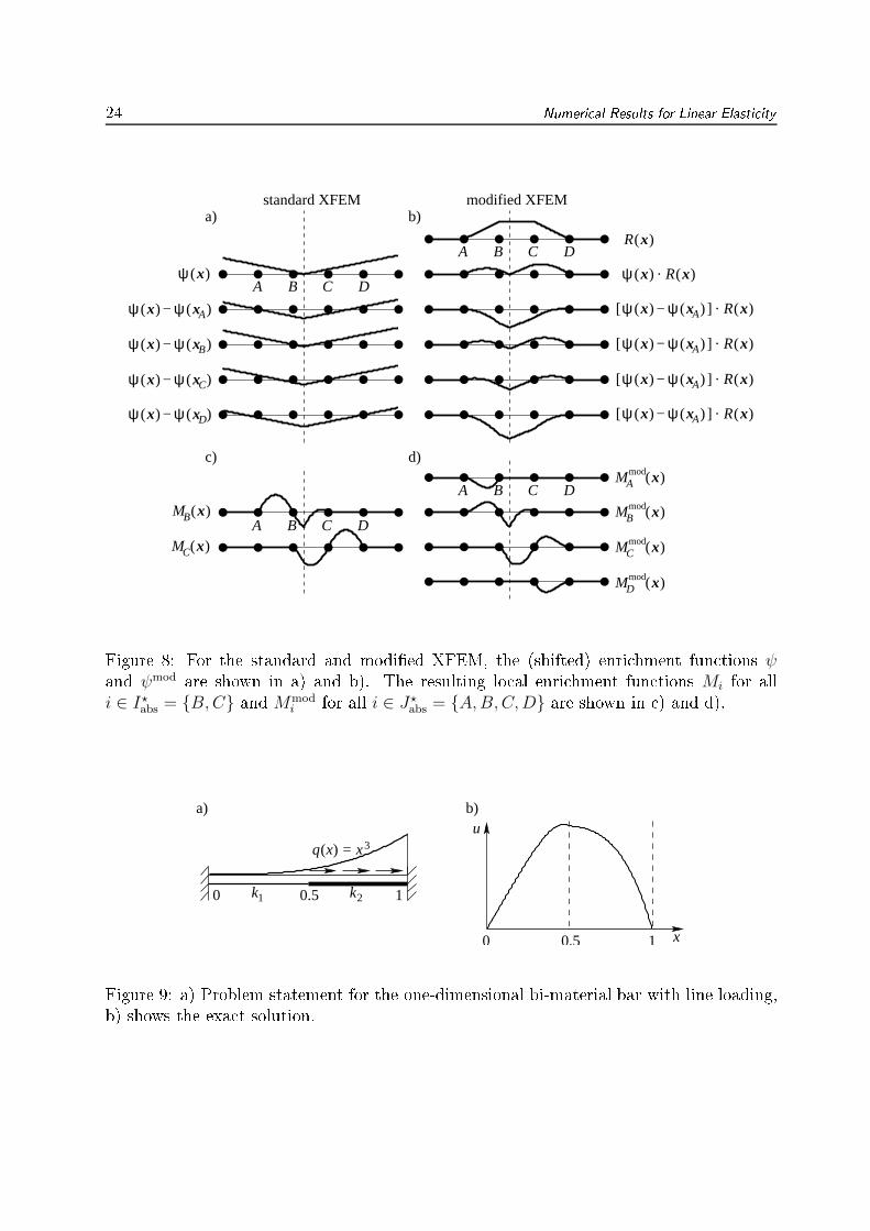
4.3 One-dimensional Bar: Convergen e Study 23For the proposed modied XFEM, the lo al enri hment fun tions areMmod

i (x) = N⋆i (x) ·

[abs

(φh (x)

)− abs

(φh (xi)

)]· R (x) ∀i ∈ J⋆

abs. (4.10)It an be seen that there are more enri hment fun tions and onsequently more unknowns aithan for the standard XFEM, see (4.9). A graphi al representation of the lo al enri hmentfun tions is given in Fig. 8(d). In the reprodu ing elements, the situation is un hangedand the exa t solution (4.8) an be reprodu ed exa tly. In the blending elements, wherethe exa t solution is linear, the additional lo al enri hment fun tions MmodA and Mmod

D arepresent. It an already be seen from the visualizations of the lo al enri hment fun tions inFig. 8(d) that MmodA is able to ompensate for the fun tional ontribution of Mmod

B in theblending element A− B, and MmodD for the ontribution of Mmod

C in the blending elementC − D. Therefore, a linear fun tion an be reprodu ed exa tly in the blending elementsopposed to the situation for the standard XFEM. Most importantly, this property enablesthe modied XFEM to reprodu e the exa t solution (4.8) exa tly in the overall domain.With the modied XFEM, the exa t solution is found for this test ase for any number ofelements (the L2-error is of order 10−14).4.3 One-dimensional Bar: Convergen e StudyA onvergen e study is performed for the bi-material bar of se tion 4.2, a problem statementis given in Fig. 9(a). A ubi line for e q (x) = x3 is present along the bar of length l = 1.The problem is governed by the equation

k (x) · u,xx (x) = −q (x) , ∀x ∈ (0, 1) , (4.11)with k (x) = k1 = 1 for 0 ≤ x ≤ 0.5 and k (x) = k2 = 10 for 0.5 < x ≤ 1. Thedispla ements are pres ribed as u (0) = u (1) = 0. The exa t solution isu (x) =

− 1320

· x · 16x4(k1+k2)−31k1−k2

k1(k1+k2)for 0 ≤ x ≤ 0.5,

− 1320

· 16x5(k1+k2)−31k1x−k2x+15(k1−k2)k2(k1+k2)

for 0.5 < x ≤ 1,(4.12)and is displayed in Fig. 9(b).For the onvergen e study, nite element fun tions of dierent orders have been employed inthe standard (Ni) and enri hed part (N⋆

i ) of the XFEM approximation. Let n be the order

24 Numeri al Results for Linear Elasti ity

ψ x(ψ A)−[ ]x)( . R x)(

ψ x(ψ A)−[ ]x)( . R x)(

ψ x(ψ A)−[ ]x)( . R x)(

x)(ψ . R x)(

R x)(

ψ x(ψ A)−[ ]x)( . R x)(

x)(ψ x(ψ C)−

x)(ψ (ψ B)− x

x)(ψ x(ψ A)−

x)(ψ

ψ x(ψ D)−x)(

)(M xB

)(M xC

)(xmodMB

)(xmodMC

)(xmodMD

)(xmodMA

modified XFEMstandard XFEM

B C DA

B C DA

B C DA

B C DA

a)

c) d)

b)

Figure 8: For the standard and modied XFEM, the (shifted) enri hment fun tions ψand ψmod are shown in a) and b). The resulting lo al enri hment fun tions Mi for alli ∈ I⋆

abs = B,C and Mmodi for all i ∈ J⋆

abs = A,B,C,D are shown in ) and d).k2k1

q( )x = x3

x

ub)a)

0.5 10

0.5 10

Figure 9: a) Problem statement for the one-dimensional bi-material bar with line loading,b) shows the exa t solution.

4.4 Two-dimensional Bi-material Problem 25of the shape fun tions Ni and n⋆ the order of the partition of unity fun tions N⋆i . In therst study, n = n⋆ in the reprodu ing element. It is noted that N⋆

i is always hosen linearin the blending elements in order to avoid linear dependen ies as a result of this spe ialenri hment (abs-enri hment and linear levelset fun tion). The ramp fun tion R (x) resultsfrom a summation of the fun tions N⋆i , see Eq. (2.6), i.e. it is of order n = n⋆. Fig. 10(a)shows that, with the orre ted XFEM, optimal onvergen e is a hieved for dierent orders.Be ause the exa t solution (4.12) is a fth-order polynomial, elements with a larger orderthan 4 an nd the solution exa tly, i.e. with ma hine a ura y. In ontrast, the standardXFEM redu es to rst order a uar y for all types of elements, see Fig. 10(b). However, itis mentioned that optimal onvergen e an also be obtained for this spe i enri hment ina standard XFEM approximation by hoosing n⋆ = n − 1, i.e. the order of N⋆

i is one lessthan the order of Ni. Be ause then the unwanted terms in the blending elements may be ompensated by the standard nite element part of the approximation.In a se ond study, we set n⋆ = 1 and only n is hanged, i.e. the partition of unity fun tionsN⋆

i are kept linear. Only here, the ramp fun tion is built by the fun tions Ni in ontrastto N⋆i , onsequently R (x) is of order n for this study. The results are given in Fig. 10( ).It may be seen that the rate of onvergen e is bounded by 3.5 in the L2-norm. This an be explained from an analysis of the reprodu ing element. In the ase when n⋆ = 1independently of n, in the reprodu ing element, a polynomial of order n plus a bi-linear ontribution with a kink at x = 0.5 an be reprodu ed exa tly. However, the exa t solution(4.12) onsists of two independent fth order polynomials in ea h of the two halves whi hare C0- ontinuous at x = 0.5. It is noted that the hoi e n⋆ = n enables the representationof two independent ( ontinuous) polynomials in the reprodu ing element.

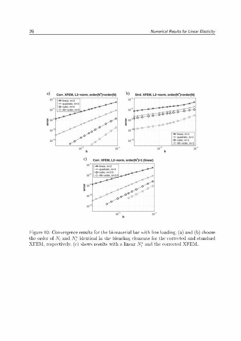
4.4 Two-dimensional Bi-material ProblemIn this test ase, a weak dis ontinuity is present, and the displa ement eld is ontinuouswith dis ontinuous stresses and strains. Inside a ir ular plate of radius b, whose materialis dened by E1 = 10 and ν1 = 0.3, a ir ular in lusion with radius a of a dierent materialwith E2 = 1 and ν2 = 0.25 is onsidered. The loading of the stru ture results from alinear displa ement of the outer boundary: ur (b, θ) = r and uθ (b, θ) = 0. The situation isdepi ted in Fig. 11(a). The exa t solution may be found in [17.

26 Numeri al Results for Linear Elasti ity

10−2

10−1

10−12

10−10

10−8

10−6

10−4

h

erro

r

Corr. XFEM, L2−norm, order(N * )=order(N)

linear, m=2quadratic, m=3cubic, m=44th−order, m=5

10−2

10−1

10−12

10−10

10−8

10−6

10−4

h

erro

r

Strd. XFEM, L2−norm, order(N * )=order(N)

linear, m=1quadratic, m=1cubic, m=14th−order, m=1

10−2

10−1

10−12

10−10

10−8

10−6

10−4

h

erro

r

Corr. XFEM, L2−norm, order(N * )=1 (linear)

linear, m=2quadratic, m=3cubic, m=3.54th−order, m=3.5

b)a)

c)

Figure 10: Convergen e results for the bi-material bar with line loading, (a) and (b) hoosethe order of Ni and N⋆i identi al in the blending elements for the orre ted and standardXFEM, respe tively, ( ) shows results with a linear N⋆

i and the orre ted XFEM.

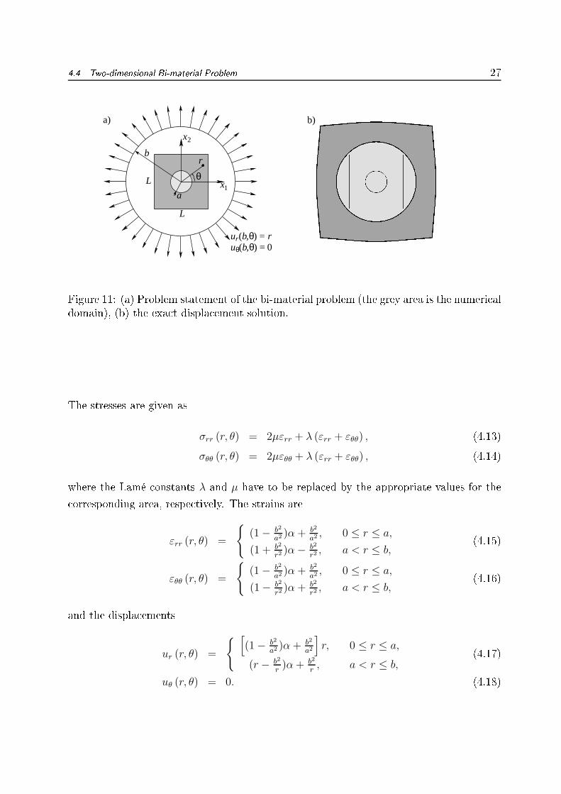
4.4 Two-dimensional Bi-material Problem 27b)a)

2

1

r

θ

,( ,( ) =

) = 0

r

x

L

L

b

x

a

θ

b θb θ

uu

r

Figure 11: (a) Problem statement of the bi-material problem (the grey area is the numeri aldomain), (b) the exa t displa ement solution.The stresses are given as

σrr (r, θ) = 2µεrr + λ (εrr + εθθ) , (4.13)σθθ (r, θ) = 2µεθθ + λ (εrr + εθθ) , (4.14)where the Lamé onstants λ and µ have to be repla ed by the appropriate values for the orresponding area, respe tively. The strains are

εrr (r, θ) =

(1 − b2

a2 )α + b2

a2 , 0 ≤ r ≤ a,

(1 + b2

r2 )α− b2

r2 , a < r ≤ b,(4.15)

εθθ (r, θ) =

(1 − b2

a2 )α + b2

a2 , 0 ≤ r ≤ a,

(1 − b2

r2 )α + b2

r2 , a < r ≤ b,(4.16)and the displa ements

ur (r, θ) =

[

(1 − b2

a2 )α + b2

a2

]

r, 0 ≤ r ≤ a,

(r − b2

r)α+ b2

r, a < r ≤ b,

(4.17)uθ (r, θ) = 0. (4.18)

28 Numeri al Results for Linear Elasti ityThe parameter α involved in these denitions isα =

(λ1 + µ1 + µ2) b2

(λ2 + µ2) a2 + (λ1 + µ1) (b2 − a2) + µ2b2. (4.19)For the numeri al model, the domain is a square of size L × L with L = 2, the outerradius is hosen to be b = 2 and the inner radius a = 0.4 + γ. The parameter γ is setto 10−3, and avoids for the meshes used that the levelset fun tion is exa tly zero at anode (in this ase, the dis ontinuity would dire tly ut through that node). The exa tstresses are pres ribed along the boundaries of the square domain, and displa ements arepres ribed as u1 (0,±1) = 0 and u2 (±1, 0) = 0. Plane strain onditions are assumed. Forthe XFEM simulation, the standard FE approximation for the displa ements is enri hedby the abs-fun tion of the levelset fun tion as des ribed in se tion 3.2.1.

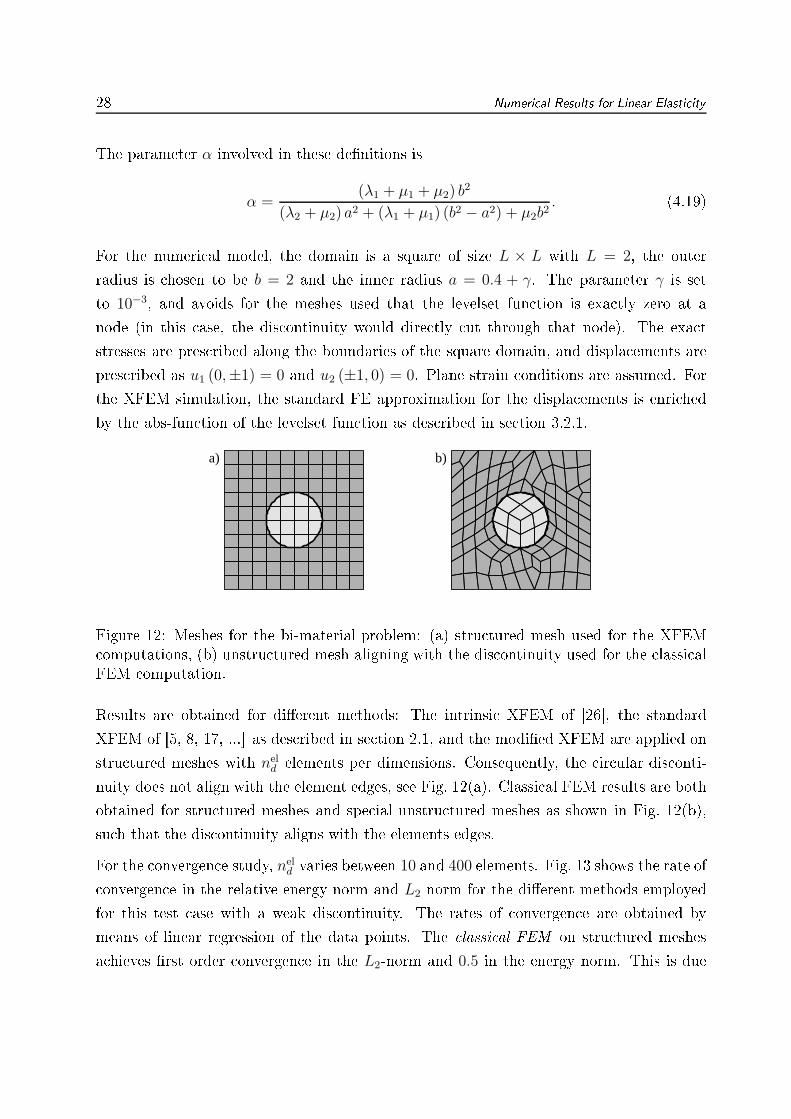
a) b)

Figure 12: Meshes for the bi-material problem: (a) stru tured mesh used for the XFEM omputations, (b) unstru tured mesh aligning with the dis ontinuity used for the lassi alFEM omputation.Results are obtained for dierent methods: The intrinsi XFEM of [26, the standardXFEM of [5, 8, 17, ... as des ribed in se tion 2.1, and the modied XFEM are applied onstru tured meshes with neld elements per dimensions. Consequently, the ir ular dis onti-nuity does not align with the element edges, see Fig. 12(a). Classi al FEM results are bothobtained for stru tured meshes and spe ial unstru tured meshes as shown in Fig. 12(b),su h that the dis ontinuity aligns with the elements edges.For the onvergen e study, nel

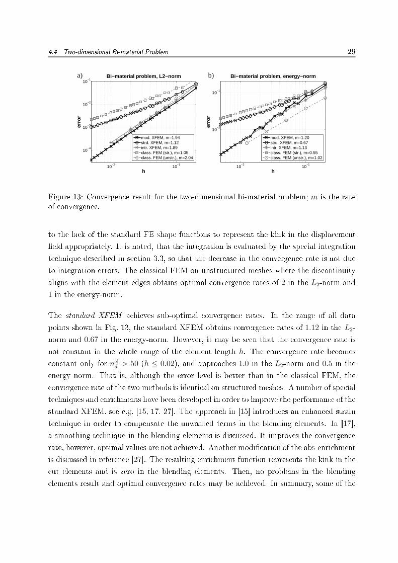
d varies between 10 and 400 elements. Fig. 13 shows the rate of onvergen e in the relative energy-norm and L2-norm for the dierent methods employedfor this test ase with a weak dis ontinuity. The rates of onvergen e are obtained bymeans of linear regression of the data points. The lassi al FEM on stru tured meshesa hieves rst order onvergen e in the L2-norm and 0.5 in the energy norm. This is due

4.4 Two-dimensional Bi-material Problem 29

10−2

10−1

10−2

10−1

h

erro

r

Bi−material problem, energy−norm

mod. XFEM, m=1.20strd. XFEM, m=0.67intr. XFEM, m=1.13class. FEM (str.), m=0.55class. FEM (unstr.), m=1.02

10−2

10−1

10−4

10−3

10−2

10−1

h

erro

rBi−material problem, L2−norm

mod. XFEM, m=1.94strd. XFEM, m=1.12intr. XFEM, m=1.89class. FEM (str.), m=1.05class. FEM (unstr.), m=2.04

b)a)

Figure 13: Convergen e result for the two-dimensional bi-material problem; m is the rateof onvergen e.to the la k of the standard FE shape fun tions to represent the kink in the displa ementeld appropriately. It is noted, that the integration is evaluated by the spe ial integrationte hnique des ribed in se tion 3.3, so that the de rease in the onvergen e rate is not dueto integration errors. The lassi al FEM on unstru tured meshes where the dis ontinuityaligns with the element edges obtains optimal onvergen e rates of 2 in the L2-norm and1 in the energy-norm.The standard XFEM a hieves sub-optimal onvergen e rates. In the range of all datapoints shown in Fig. 13, the standard XFEM obtains onvergen e rates of 1.12 in the L2-norm and 0.67 in the energy-norm. However, it may be seen that the onvergen e rate isnot onstant in the whole range of the element length h. The onvergen e rate be omes onstant only for nel

d > 50 (h ≤ 0.02), and approa hes 1.0 in the L2-norm and 0.5 in theenergy norm. That is, although the error level is better than in the lassi al FEM, the onvergen e rate of the two methods is identi al on stru tured meshes. A number of spe ialte hniques and enri hments have been developed in order to improve the performan e of thestandard XFEM, see e.g. [15, 17, 27. The approa h in [15 introdu es an enhan ed strainte hnique in order to ompensate the unwanted terms in the blending elements. In [17,a smoothing te hnique in the blending elements is dis ussed. It improves the onvergen erate, however, optimal values are not a hieved. Another modi ation of the abs-enri hmentis dis ussed in referen e [27. The resulting enri hment fun tion represents the kink in the ut elements and is zero in the blending elements. Then, no problems in the blendingelements result and optimal onvergen e rates may be a hieved. In summary, some of the

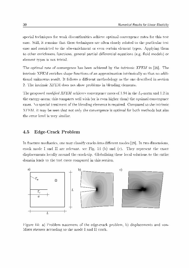
30 Numeri al Results for Linear Elasti ityspe ial te hniques for weak dis ontinuities a hieve optimal onvergen e rates for this test ase. Still, it remains that these te hniques are often losely related to the parti ular test ase and restri ted to the abs-enri hment or even ertain element types. Applying themto other enri hment fun tions, general partial dierential equations (e.g. uid models) orelement types is not trivial.The optimal rate of onvergen e has been a hieved by the intrinsi XFEM in [26. Theintrinsi XFEM enri hes shape fun tions of an approximation intrinsi ally so that no addi-tional unknowns result. It follows a dierent methodology as the one des ribed in se tion2. The intrinsi XFEM does not show problems in blending elements.The proposed modied XFEM a hieves onvergen e rates of 1.94 in the L2-norm and 1.2 inthe energy-norm; this ompares well with (or is even higher than) the optimal onvergen erates. No spe ial treatment of the blending elements is required. Compared to the intrinsi XFEM, it may be seen that not only the onvergen e is optimal for both methods but alsothe error level is very similar.4.5 Edge-Cra k ProblemIn fra ture me hani s, one may lassify ra ks into dierent modes [28. In two dimensions, ra k mode I and II are relevant, see Fig. 14 (b) and ( ). They represent the exa tdispla ements lo ally around the ra k-tip. Globalizing these lo al solutions to the entiredomain leads to the test ases omputed in this se tion.Γc

Γu

a)

L

Ω

L

a

b) c)

Figure 14: a) Problem statement of the edge- ra k problem, b) displa ements and von-Mises stresses a ording to the mode I and II ra k.

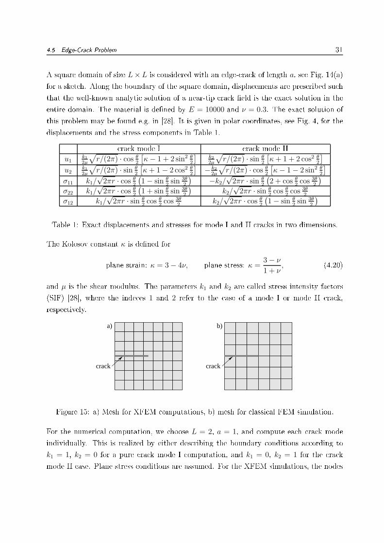
4.5 Edge-Cra k Problem 31A square domain of size L×L is onsidered with an edge- ra k of length a, see Fig. 14(a)for a sket h. Along the boundary of the square domain, displa ements are pres ribed su hthat the well-known analyti solution of a near-tip ra k eld is the exa t solution in theentire domain. The material is dened by E = 10000 and ν = 0.3. The exa t solution ofthis problem may be found e.g. in [28. It is given in polar oordinates, see Fig. 4, for thedispla ements and the stress omponents in Table 1. ra k mode I ra k mode IIu1

k1

2µ

√

r/(2π) · cos θ2

[κ− 1 + 2 sin2 θ

2

]k2

2µ

√

r/(2π) · sin θ2

[κ+ 1 + 2 cos2 θ

2

]

u2k1

2µ

√

r/(2π) · sin θ2

[κ + 1 − 2 cos2 θ

2

]− k2

2µ

√

r/(2π) · cos θ2

[κ− 1 − 2 sin2 θ

2

]

σ11 k1/√

2πr · cos θ2

(1 − sin θ

2sin 3θ

2

)−k2/

√2πr · sin θ

2

(2 + cos θ

2cos 3θ

2

)

σ22 k1/√

2πr · cos θ2

(1 + sin θ

2sin 3θ

2

)k2/

√2πr · sin θ

2cos θ

2cos 3θ

2

σ12 k1/√

2πr · sin θ2cos θ

2cos 3θ

2k2/

√2πr · cos θ

2

(1 − sin θ

2sin 3θ

2

)Table 1: Exa t displa ements and stresses for mode I and II ra ks in two dimensions.The Kolosov onstant κ is dened forplane strain: κ = 3 − 4ν, plane stress: κ =3 − ν

1 + ν, (4.20)and µ is the shear modulus. The parameters k1 and k2 are alled stress intensity fa tors(SIF) [28, where the inde es 1 and 2 refer to the ase of a mode I or mode II ra k,respe tively.

a) b)

crack crack

Figure 15: a) Mesh for XFEM omputations, b) mesh for lassi al FEM simulation.For the numeri al omputation, we hoose L = 2, a = 1, and ompute ea h ra k modeindividually. This is realized by either des ribing the boundary onditions a ording tok1 = 1, k2 = 0 for a pure ra k mode I omputation, and k1 = 0, k2 = 1 for the ra kmode II ase. Plane stress onditions are assumed. For the XFEM simulations, the nodes

32 Numeri al Results for Linear Elasti ityaround the ra k-tip within an radius of rtip are enri hed with the bran h fun tions asdes ribed in se tion 3.2.3. Along the ra k, the sign-enri hment is used as dis ussed inse tion 3.2.2. Only stru tured meshes have been used with neld elements per dimension.For the onvergen e study with dierent XFEM approa hes, nel

d is an odd number between9 and 399, onsequently, the dis ontinuity never aligns with the elements, see Fig. 15(a).For omputations with the lassi al FEM, nel

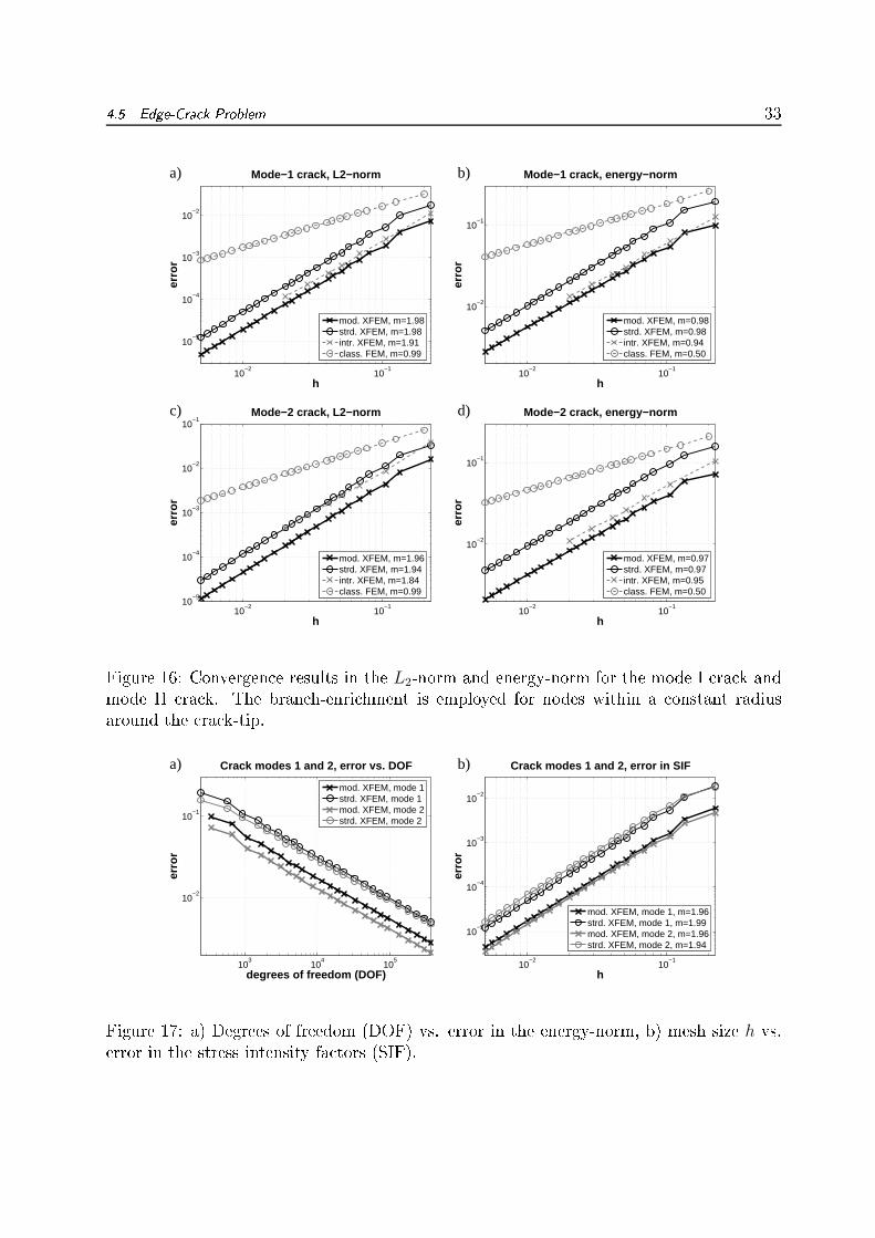
d is an even number between 10 and 400 sothat the ra k aligns with the element edges and a node is pla ed dire tly at the ra k-tip,see Fig. 15(b).4.5.1 Bran h-enri hment with Constant RadiusThe rst results are obtained for a onstant radius rtip = 0.2 around the ra k-tip. Nodeswithin this radius are enri hed as des ribed in se tion 3.2.3. Fig. 16 shows the rates of onvergen e in the energy and L2-norm obtained with the standard, intrinsi , and modiedXFEM and lassi al FEM for this test ase with a strong dis ontinuity.By means of the lassi al FEM only a redu ed onvergen e order of 1 in the L2-norm and0.5 in the energy-norm is a hieved although the ra k aligns with the element edges and anode is pla ed at the ra k-tip. The reason an be found in the singularity of the stressesand strains at the ra k-tip whi h inhibits higher onvergen e rates, see also [3.All three XFEM alternativesstandard, intrinsi , and modied XFEMa hieve optimal onvergen e of 2 in the L2-norm and 1 in the energy-norm. It is surprising that for thestandard XFEM, the undesired terms that are present in the blending elements of thebran h-enri hment, see se tion 2.2, do not seem to de rease the onvergen e as was the ase for the previous test ase with the abs-enri hment. Comparing the error-levels of theresults shows that for the same element size h, the proposed modied XFEM is better bya fa tor of 3 to 5 than the standard XFEM.The modied XFEM enri hes more unknowns than the standard XFEM. Therefore, inFig. 17(a), the degrees of freedom (DOF) are ompared between the standard and modiedXFEM for the two ra k modes. It an be seen that for a given a ura y, the modiedXFEM requires about 3 times less degrees of freedom than the standard XFEM.The stress intensity fa tors k1 and k2 have been evaluated numeri ally in a radial integrationdomain of radius r = 0.6 around the ra k-tip. The intera tion integral is evaluated forthis purpose, see [8, and the fa tors should be onstant, independent of the integration

4.5 Edge-Cra k Problem 33

10−2

10−1

10−5

10−4

10−3

10−2

h

erro

rMode−1 crack, L2−norm

mod. XFEM, m=1.98strd. XFEM, m=1.98intr. XFEM, m=1.91class. FEM, m=0.99

10−2

10−1

10−2

10−1

h

erro

r

Mode−1 crack, energy−norm

mod. XFEM, m=0.98strd. XFEM, m=0.98intr. XFEM, m=0.94class. FEM, m=0.50

b)a)

10−2

10−1

10−5

10−4

10−3

10−2

10−1

h

erro

r

Mode−2 crack, L2−norm

mod. XFEM, m=1.96strd. XFEM, m=1.94intr. XFEM, m=1.84class. FEM, m=0.99

10−2

10−1

10−2

10−1

h

erro

r

Mode−2 crack, energy−norm

mod. XFEM, m=0.97strd. XFEM, m=0.97intr. XFEM, m=0.95class. FEM, m=0.50

d)c)

Figure 16: Convergen e results in the L2-norm and energy-norm for the mode I ra k andmode II ra k. The bran h-enri hment is employed for nodes within a onstant radiusaround the ra k-tip.

103

104

105

10−2

10−1

degrees of freedom (DOF)

erro

r

Crack modes 1 and 2, error vs. DOF

mod. XFEM, mode 1strd. XFEM, mode 1mod. XFEM, mode 2strd. XFEM, mode 2

10−2

10−1

10−5

10−4

10−3

10−2

h

erro

r

Crack modes 1 and 2, error in SIF

mod. XFEM, mode 1, m=1.96strd. XFEM, mode 1, m=1.99mod. XFEM, mode 2, m=1.96strd. XFEM, mode 2, m=1.94

b)a)

Figure 17: a) Degrees of freedom (DOF) vs. error in the energy-norm, b) mesh size h vs.error in the stress intensity fa tors (SIF).

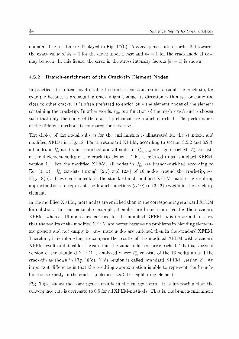
34 Numeri al Results for Linear Elasti itydomain. The results are displayed in Fig. 17(b). A onvergen e rate of order 2.0 towardsthe exa t value of k1 = 1 for the ra k mode I ase and k2 = 1 for the ra k mode II asemay be seen. In this gure, the error in the stress intensity fa tors |ki − 1| is shown.4.5.2 Bran h-enri hment of the Cra k-tip Element NodesIn pra ti e, it is often not desirable to enri h a onstant radius around the ra k tip, forexample be ause a propagating ra k might hange its dire tion within rtip or ome too lose to other ra ks. It is often preferred to enri h only the element nodes of the element ontaining the ra k-tip. In other words, rtip is a fun tion of the mesh size h and is hosensu h that only the nodes of the ra k-tip element are bran h-enri hed. The performan eof the dierent methods is ompared for this ase.The hoi e of the nodal subsets for the enri hments is illustrated for the standard andmodied XFEM in Fig. 18. For the standard XFEM, a ording to se tion 3.2.2 and 3.2.3,all nodes in I⋆br are bran h-enri hed and all nodes in I⋆

sign,red are sign-enri hed. I⋆br onsistsof the 4 element nodes of the ra k-tip element. This is referred to as standard XFEM,version 1. For the modied XFEM, all nodes in J⋆

br are bran h-enri hed a ording toEq. (3.15). J⋆br onsists through (2.7) and (2.8) of 16 nodes around the ra k-tip, seeFig. 18(b). These enri hments in the standard and modied XFEM enable the resultingapproximations to represent the bran h-fun tions (3.10) to (3.13) exa tly in the ra k-tipelement.In the modied XFEM, more nodes are enri hed than in the orresponding standard XFEMformulation. In this parti ular example, 4 nodes are bran h-enri hed for the standardXFEM, whereas 16 nodes are enri hed for the modied XFEM. It is important to showthat the results of the modied XFEM are better be ause no problems in blending elementsare present and not simply be ause more nodes are enri hed than in the standard XFEM.Therefore, it is interesting to ompare the results of the modied XFEM with standardXFEM results obtained for the ase that the same nodal sets are enri hed. That is, a se ondversion of the standard XFEM is analyzed where I⋆

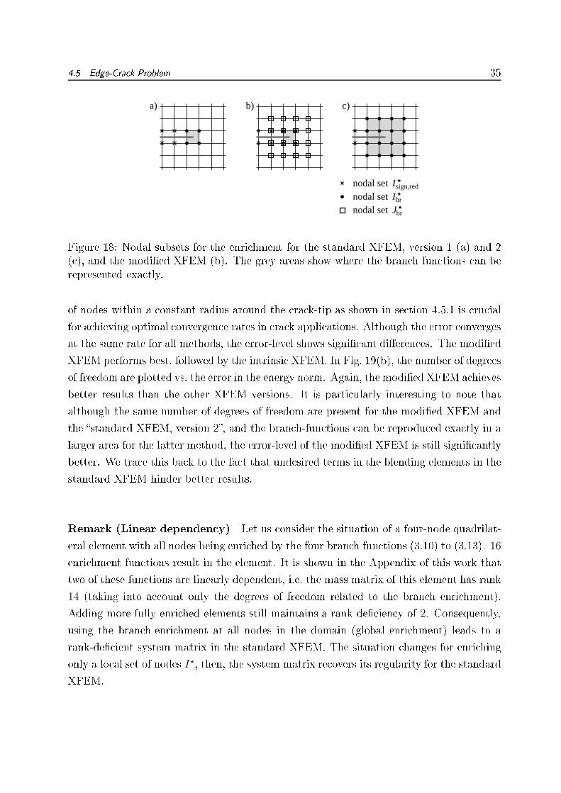
br onsists of the 16 nodes around the ra k-tip as shown in Fig. 18( ). This version is alled standard XFEM, version 2. Animportant dieren e is that the resulting approximation is able to represent the bran h-fun tions exa tly in the ra k-tip element and its neighboring elements.Fig. 19(a) shows the onvergen e results in the energy norm. It is interesting that the onvergen e rate is de reased to 0.5 for all XFEM-methods. That is, the bran h-enri hment

4.5 Edge-Cra k Problem 35nodal set br

Inodal setJ

br

nodal set sign,redI

a) c)b)

Figure 18: Nodal subsets for the enri hment for the standard XFEM, version 1 (a) and 2( ), and the modied XFEM (b). The grey areas show where the bran h fun tions an berepresented exa tly.of nodes within a onstant radius around the ra k-tip as shown in se tion 4.5.1 is ru ialfor a hieving optimal onvergen e rates in ra k appli ations. Although the error onvergesat the same rate for all methods, the error-level shows signi ant dieren es. The modiedXFEM performs best, followed by the intrinsi XFEM. In Fig. 19(b), the number of degreesof freedom are plotted vs. the error in the energy norm. Again, the modied XFEM a hievesbetter results than the other XFEM versions. It is parti ularly interesting to note thatalthough the same number of degrees of freedom are present for the modied XFEM andthe standard XFEM, version 2, and the bran h-fun tions an be reprodu ed exa tly in alarger area for the latter method, the error-level of the modied XFEM is still signi antlybetter. We tra e this ba k to the fa t that undesired terms in the blending elements in thestandard XFEM hinder better results.Remark (Linear dependen y) Let us onsider the situation of a four-node quadrilat-eral element with all nodes being enri hed by the four bran h fun tions (3.10) to (3.13). 16enri hment fun tions result in the element. It is shown in the Appendix of this work thattwo of these fun tions are linearly dependent, i.e. the mass matrix of this element has rank14 (taking into a ount only the degrees of freedom related to the bran h enri hment).Adding more fully enri hed elements still maintains a rank de ien y of 2. Consequently,using the bran h-enri hment at all nodes in the domain (global enri hment) leads to arank-de ient system matrix in the standard XFEM. The situation hanges for enri hingonly a lo al set of nodes I⋆, then, the system matrix re overs its regularity for the standardXFEM.

36 Numeri al Results for Linear Elasti ity

10−2

10−1

10−2

10−1

h

erro

rMode−1 crack, energy−norm

mod. XFEMstrd. XFEM 1strd. XFEM 2intr. XFEMclass. FEM

103

104

105

10−2

10−1

degrees of freedom (DOF)

erro

r

Mode−1 crack, error vs. DOF

mod. XFEMstrd. XFEM 1strd. XFEM 2intr. XFEMclass. FEM

b)a)

Figure 19: Convergen e results in the energy-norm for bran h-enri hment only in the losevi inity of the ra k-tip element, a) mesh size h vs. error, b) degrees of freedom (DOF) vs.error.In ontrast, for the modied XFEM, the rank-de ien y also remains for lo al enri hmentsbe ause all the nodes of the blending and reprodu ing elements are enri hed, see theAppendix of this work. One an easily ir umvent problems by eliminating two equationsresulting for the bran h-enri hed degrees of freedom in the nal system matrix. All resultsshown above have been obtained after this elimination. We on lude that this problem isnot inherent in the proposed modi ation of the XFEM but stems from the parti ular aseof the bran h-enri hment.Remark (Optimal onvergen e) We found that the following aspe ts have to be onsidered in order to obtain optimal onvergen e (for standard, intrinsi , and modiedXFEM) in this test ase:• The integration rule in the ra k-tip element is ru ial for the su ess. The almostpolar integration, see se tion 3.3, is one way to integrate appropriately, see e.g. [16.• The radius of the bran h-enri hment has to be kept onstant throughout the onver-gen e study as e.g. also noted in [16, 25.• In the standard and modied XFEM, attention has to be paid for the ase where theenri hment fun tionsMi (x) andMmod

i (x) are non-zero along the Diri hlet boundary.Then, apart from pres ribing the unknowns ui along the Diri hlet boundary, theboundary term ∫wh · th

dΓ, see Eq. (4.6), still has to be evaluated for the enri hmentfun tions. See also [29 for imposing Diri hlet boundary onditions in the XFEM.

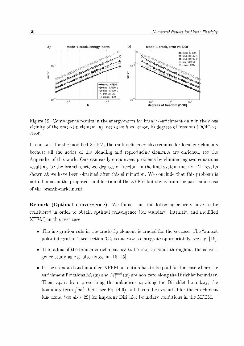
37Remark (Other modied XFEM approximations) In [16, two modi ations ofthe standard XFEM approximation have been proposed for the spe ial ase of ra k ap-pli ations. The approa h of [16, se tion 5.1, diers from the approximation proposed inthis work by the fa t that only the standard nodal set I⋆ is enri hed; suboptimal resultsare obtained. The other approa h of [16, se tion 5.5, ouples enri hed and standard FEapproximations pointwise at the nodes, its motivation is the redu tion of the blendingelement area to zero. The formulation of the approximation and the enri hment fun tionsare dierent from the proposed approximation. It is noted, that for the se ond approa h,optimal onvergen e has been a hieved for ra k appli ations.5 Summary and Con lusionsThe standard formulation of XFEM approximations leads to problems in blending elements.Unwanted terms are introdu ed whi h may de rease the overall onvergen e. The ee t ofthe unwanted terms in the blending elements depends on the parti ular enri hment hosen.For the numeri al studies ondu ted in this work, it was found that for the abs-enri hment,the blending elements ause a severe redu tion of the onvergen e rate to the same ratethat an be a hieved without any enri hment. For the bran h-enri hment, the optimal onvergen e rate was maintained, however, the error was signi antly larger than in the orresponding orre ted XFEM. We on lude that blending elements have an importantbut hard to predi t inuen e on the a ura y of an approximation. For the developmentof new enri hment fun tions in the ontext of the standard XFEMe.g. for sho ks andboundary layers in uid me hani sthis means that an enri hment is only useful if (i) thelo al solution hara teristi s are onsidered appropriately and (ii) it an be shown (e.g. bynumeri al observation) that the problems in blending elements are not dominating theoverall a ura y.In ontrast, for the proposed modied XFEM approximation, no problems in the blendingelements result. This is a hieved by a modi ation of the enri hment fun tions and anenri hment of all nodes in the blending elements. The proposed modi ation works forarbitrary enri hments, and is not limited to ertain element types and partial dierentialequations. The modied XFEM approximation is easily in luded in existing XFEM odes.The overall number of degrees of freedom is slightly in reased ompared to a standardXFEM omputation.

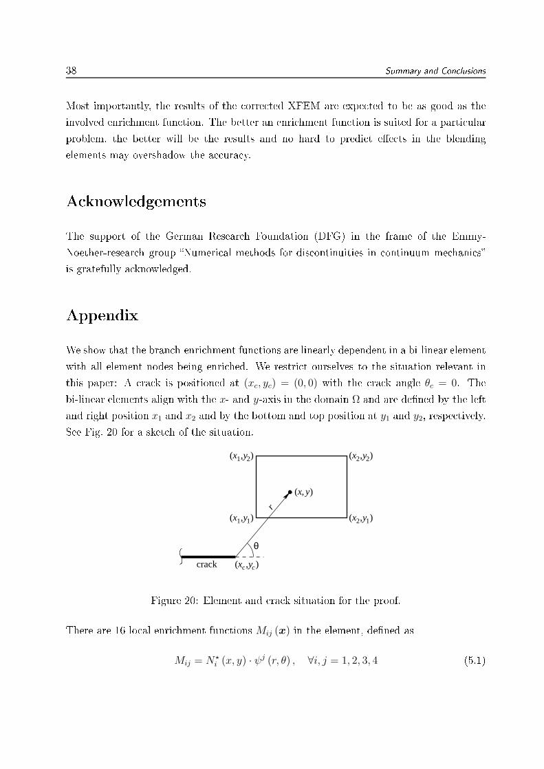
38 Summary and Con lusionsMost importantly, the results of the orre ted XFEM are expe ted to be as good as theinvolved enri hment fun tion. The better an enri hment fun tion is suited for a parti ularproblem, the better will be the results and no hard to predi t ee ts in the blendingelements may overshadow the a ura y.A knowledgementsThe support of the German Resear h Foundation (DFG) in the frame of the Emmy-Noether-resear h group Numeri al methods for dis ontinuities in ontinuum me hani sis gratefully a knowledged.AppendixWe show that the bran h-enri hment fun tions are linearly dependent in a bi-linear elementwith all element nodes being enri hed. We restri t ourselves to the situation relevant inthis paper: A ra k is positioned at (xc, yc) = (0, 0) with the ra k angle θc = 0. Thebi-linear elements align with the x- and y-axis in the domain Ω and are dened by the leftand right position x1 and x2 and by the bottom and top position at y1 and y2, respe tively.See Fig. 20 for a sket h of the situation.x( ,y)

yx( ),c c

)yx( ,1 2 yx( ),2 2

yx ,2 1yx ),1 1( ( )

crack

r

θ

Figure 20: Element and ra k situation for the proof.There are 16 lo al enri hment fun tions Mij (x) in the element, dened asMij = N⋆

i (x, y) · ψj (r, θ) , ∀i, j = 1, 2, 3, 4 (5.1)

39with ψj being the bran h fun tions given by (3.10) to (3.13), and N⋆i are the bi-linear niteelement shape fun tions

N⋆1 = (1 − ξ) (1 − η) , N⋆

3 = (ξ) (η) ,

N⋆2 = (ξ) (1 − η) , N⋆

4 = (1 − ξ) (η) ,with ξ = (x− x1) / (x2 − x1) and η = (y − y1) / (y2 − y1). We repla e x and y by x =

r · cos θ and y = r · sin θ. The 16 fun tions (5.1) are linearly independent if0 =

4∑

i=1

4∑

j=1

N⋆i (r, θ) · ψj (r, θ) · aij (5.2)only holds for aij = 0 ∀i, j.

However, it an be shown that the following hoi e of aij also fullls (5.2):aij =

y1x2/y2 x1x2/y2 + y1 −y1 −y1x2/y2 + x1

y1x2/y2 x22/y2 + y1 −y1 −y1x2/y2 + x2

x2 x22/y2 + y2 −y2 0

x2 x1x2/y2 + y2 −y2 x1 − x2

. (5.3)This oe ient matrix an be used in (5.2) in order to repla e fun tionM44 by 14 fun tionsMij . A se ond oe ient matrix

aij =

x1y1/y2 x21/y2 + y1 −y1 (y2 − y1)x1/y2

x1y1/y2 x1x2/y2 + y1 −y1 (y2 − y1)x1/y2 + x2 − x1

x1 x1x2/y2 + y2 −y2 x2 − x1

x1 x21/y2 + y2 −y2 0

. (5.4) an be used in (5.2) in order to repla e fun tion M34 by the same 14 fun tions Mij usedbefore. This shows that 2 of the 16 equations in (5.1) are linearly dependent. The samelinear ombinations given above hold for the shifted enri hment in the element a ordingto se tion 2.4, whi h givesM shift

ij = N⋆i (x) ·

[ψj (x) − ψj (xi)

], ∀i, j = 1, 2, 3, 4. (5.5)

40 REFERENCESFurthermore, they also hold for the modied, shifted enri hment fun tions, i.e. forMmod,shift

ij = N⋆i (x) ·

[ψj (x) − ψj (xi)

]· R (x) , ∀i, j = 1, 2, 3, 4. (5.6)

Referen es[1 T. Belyts hko, W.K. Liu, and B. Moran. Nonlinear Finite Elements for Continua andStru tures. John Wiley & Sons, Chi hester, 2000.[2 O.C. Zienkiewi z and R.L. Taylor. The Finite Element Method, volume 1 3.Butterworth-Heinemann, Oxford, 2000.[3 G. Strang and G. Fix. An Analysis of the Finite Element Method. Prenti e-Hall,Englewood Clis, NJ, 1973.[4 I. Babu²ka and J.M. Melenk. The partition of unity method. Internat. J. Numer.Methods Engrg., 40:727 758, 1997.[5 T. Belyts hko, N. Moës, S. Usui, and C. Parimi. Arbitrary dis ontinuities in niteelements. Internat. J. Numer. Methods Engrg., 50:993 1013, 2001.[6 T. Belyts hko and T. Bla k. Elasti ra k growth in nite elements with minimalremeshing. Internat. J. Numer. Methods Engrg., 45:601 620, 1999.[7 J.M. Melenk and I. Babu²ka. The partition of unity nite element method: Basi theory and appli ations. Comp. Methods Appl. Me h. Engrg., 139:289 314, 1996.[8 N. Moës, J. Dolbow, and T. Belyts hko. A nite element method for ra k growthwithout remeshing. Internat. J. Numer. Methods Engrg., 46:131 150, 1999.[9 J.E. Dolbow, N. Moës, and T. Belyts hko. Dis ontinuous enri hment in nite elementswith a partition of unity method. Internat. J. Numer. Methods Engrg., 36:235 260,2000.[10 C. Daux, N. Moës, J.E. Dolbow, and N. Sukumar. Arbitrary bran hed and interse ting ra ks with the extended nite element method. Internat. J. Numer. Methods Engrg.,48:1741 1760, 2000.

REFERENCES 41[11 J. Chessa, P. Smolinski, and T. Belyts hko. The extended nite element method(XFEM) for solidi ation problems. Internat. J. Numer. Methods Engrg., 53:1959 1977, 2002.[12 J. Chessa and T. Belyts hko. The extended nite element method for two-phase uids.ASME J. Appl. Me h., 70:10 17, 2003.[13 J.E. Dolbow and R. Merle. Solving thermal and phase hange problems with theextended nite element method. Comput. Me h., 28:339 350, 2002.[14 H. Ji, D. Chopp, and J.E. Dolbow. A hybrid extended nite element/level set methodfor modeling phase transformations. Internat. J. Numer. Methods Engrg., 54:1209 1233, 2002.[15 J. Chessa, H. Wang, and T. Belyts hko. On the onstru tion of blending elements forlo al partition of unity enri hed nite elements. Internat. J. Numer. Methods Engrg.,57:1015 1038, 2003.[16 P. Laborde, J. Pommier, Y. Renard, and M. Salaün. High-order extended niteelement method for ra ked domains. Internat. J. Numer. Methods Engrg., 64:354 381, 2005.[17 N. Sukumar, D.L. Chopp, N. Moës, and T. Belyts hko. Modeling holes and in lusionsby level sets in the extended nite-element method. Comp. Methods Appl. Me h.Engrg., 190:6183 6200, 2001.[18 F.L. Stazi, E. Budyn, J. Chessa, and T. Belyts hko. An extended nite elementmethod with higher-order elements for ra k problems with urvature. Comput. Me h.,31:38 48, 2003.[19 J. Chessa. The extended XFEM for free surfa e and two phase ow problems. Disser-tation, Northwestern University, 2003.[20 A. Kölke. Modellierung und Diskretisierung bewegter Diskontinuitäten in randgekop-pelten Mehrfeldaufgaben. Dissertation, Te hnis he Universität Brauns hweig, 2005.[21 A. Kölke and A. Legay. The enri hed spa e-time nite element method (EST) forsimultaneous solution of uid-stru ture intera tion. Internat. J. Numer. Methods En-grg., 0:submitted, 2007.

42 REFERENCES[22 S. Osher and R.P. Fedkiw. Level Set Methods and Dynami Impli it Surfa es. SpringerVerlag, Berlin, 2003.[23 M. Stolarska, D.L. Chopp, N. Moës, and T. Belyts hko. Modelling ra k growth bylevel sets in the extended nite element method. Internat. J. Numer. Methods Engrg.,51:943 960, 2001.[24 M. Duot. A study of the representation of ra ks with level-sets. Internat. J. Numer.Methods Engrg., 70:12611302, 2007.[25 E. Bé het, H. Minnebo, N. Moës, and B. Burgardt. Improved implementation androbustness study of the x-fem for stress analysis around ra ks. Internat. J. Numer.Methods Engrg., 64:10331056, 2005.[26 T.P. Fries and T. Belyts hko. The intrinsi XFEM: A method for arbitrary dis onti-nuities without additional unknowns. Internat. J. Numer. Methods Engrg., 68:1358 1385, 2006.[27 N. Moës, M. Cloire , P. Cartaud, and J.F. Rema le. A omputational approa hto handle omplex mi rostru ture geometries. Comp. Methods Appl. Me h. Engrg.,192:31633177, 2003.[28 H. Ewalds and R. Wanhill. Fra ture Me hani s. Edward Arnold, New York, 1989.[29 N. Moës, E. Bé het, and M. Tourbier. Imposing Diri hlet boundary onditions in theextended nite element method. Internat. J. Numer. Methods Engrg., 67:1641 1669,2006.