Embed Size (px)
Citation preview
A – 1
Copyright © 2010 Pearson Education, Inc. Publishing as Prentice Hall.
Decision MakingA
For Operations Management, 9e by Krajewski/Ritzman/Malhotra © 2010 Pearson Education
PowerPoint Slides by Jeff Heyl
A – 2
Copyright © 2010 Pearson Education, Inc. Publishing as Prentice Hall.
Break-Even Analysis
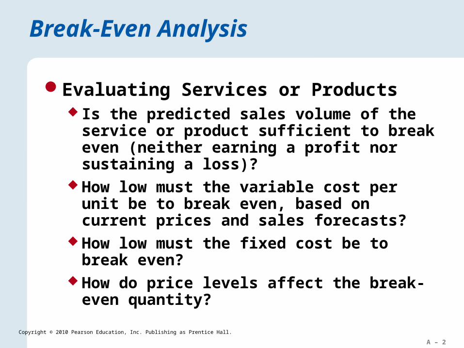
Evaluating Services or Products Is the predicted sales volume of the service or
product sufficient to break even (neither earning a profit nor sustaining a loss)?
How low must the variable cost per unit be to break even, based on current prices and sales forecasts?
How low must the fixed cost be to break even? How do price levels affect the break-even
quantity?
A – 3
Copyright © 2010 Pearson Education, Inc. Publishing as Prentice Hall.
Break-Even Analysis
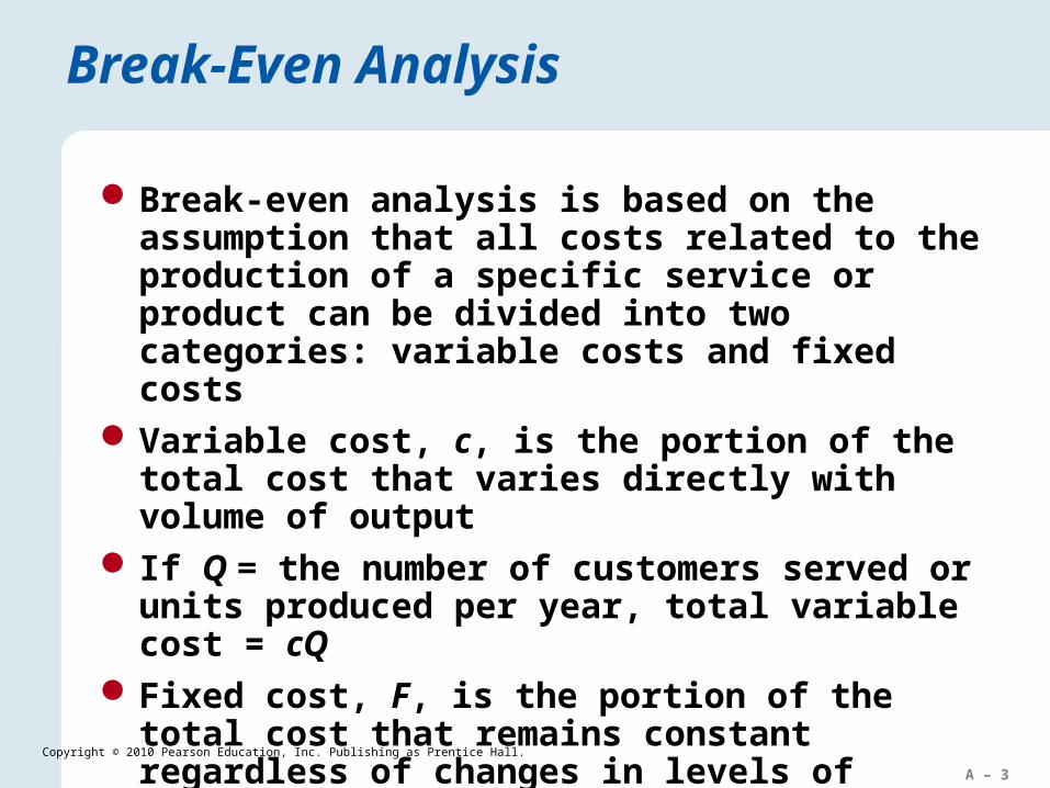
Break-even analysis is based on the assumption that all costs related to the production of a specific service or product can be divided into two categories: variable costs and fixed costs
Variable cost, c, is the portion of the total cost that varies directly with volume of output
If Q = the number of customers served or units produced per year, total variable cost = cQ
Fixed cost, F, is the portion of the total cost that remains constant regardless of changes in levels of output
A – 4
Copyright © 2010 Pearson Education, Inc. Publishing as Prentice Hall.
Break-Even Analysis
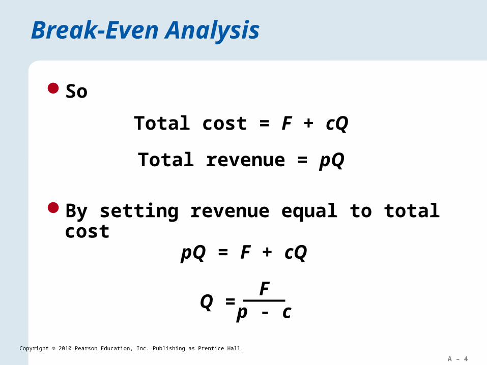
By setting revenue equal to total cost
pQ = F + cQ
Q =F
p - c
So
Total cost = F + cQ
Total revenue = pQ
A – 5
Copyright © 2010 Pearson Education, Inc. Publishing as Prentice Hall.
Finding the Break-Even Quantity
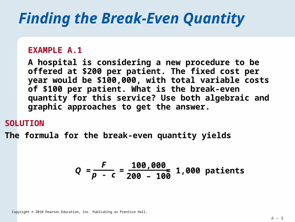
EXAMPLE A.1
A hospital is considering a new procedure to be offered at $200 per patient. The fixed cost per year would be $100,000, with total variable costs of $100 per patient. What is the break-even quantity for this service? Use both algebraic and graphic approaches to get the answer.
SOLUTION
The formula for the break-even quantity yields
Q =F
p - c = 1,000 patients=100,000
200 – 100
A – 6
Copyright © 2010 Pearson Education, Inc. Publishing as Prentice Hall.
Finding the Break-Even Quantity
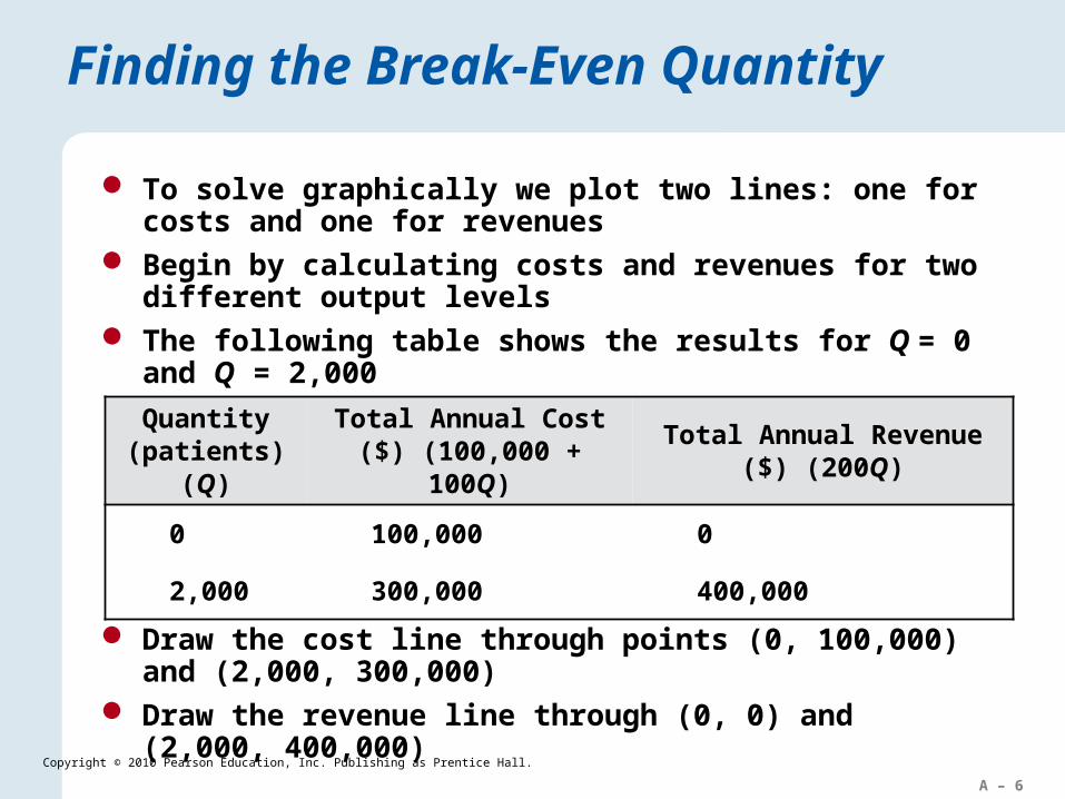
To solve graphically we plot two lines: one for costs and one for revenues
Begin by calculating costs and revenues for two different output levels
The following table shows the results for Q = 0 and Q = 2,000
Quantity (patients) (Q)
Total Annual Cost ($) (100,000 + 100Q)
Total Annual Revenue ($) (200Q)
0 100,000 0
2,000 300,000 400,000
Draw the cost line through points (0, 100,000) and (2,000, 300,000)
Draw the revenue line through (0, 0) and (2,000, 400,000)
A – 7
Copyright © 2010 Pearson Education, Inc. Publishing as Prentice Hall.
Finding the Break-Even Quantity
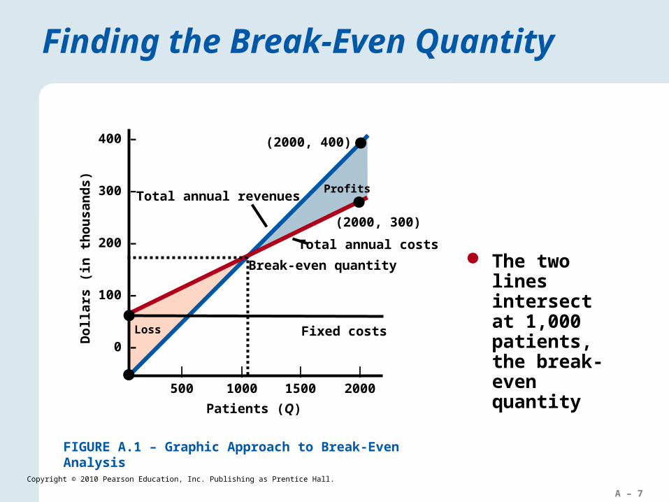
Total annual costs
Fixed costs
Break-even quantity
Profits
Loss
Patients (Q)
Do
llar
s (
in t
ho
usa
nd
s)
400 –
300 –
200 –
100 –
0 –
| | | |
500 1000 1500 2000
(2000, 300)
Total annual revenues
The two lines intersect at 1,000 patients, the break-even quantity
FIGURE A.1 – Graphic Approach to Break-Even Analysis
(2000, 400)
A – 8
Copyright © 2010 Pearson Education, Inc. Publishing as Prentice Hall.
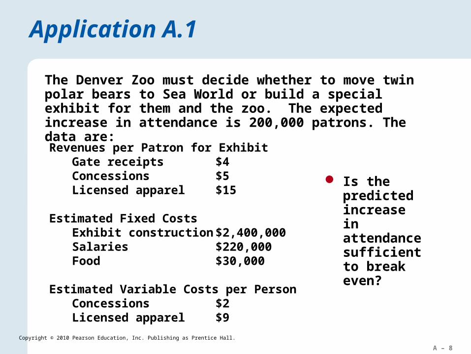
Application A.1
The Denver Zoo must decide whether to move twin polar bears to Sea World or build a special exhibit for them and the zoo. The expected increase in attendance is 200,000 patrons. The data are:
Revenues per Patron for ExhibitGate receipts $4Concessions $5Licensed apparel $15
Estimated Fixed CostsExhibit construction $2,400,000Salaries $220,000Food $30,000
Estimated Variable Costs per PersonConcessions $2Licensed apparel $9
Is the predicted increase in attendance sufficient to break even?
A – 9
Copyright © 2010 Pearson Education, Inc. Publishing as Prentice Hall.
Application A.1
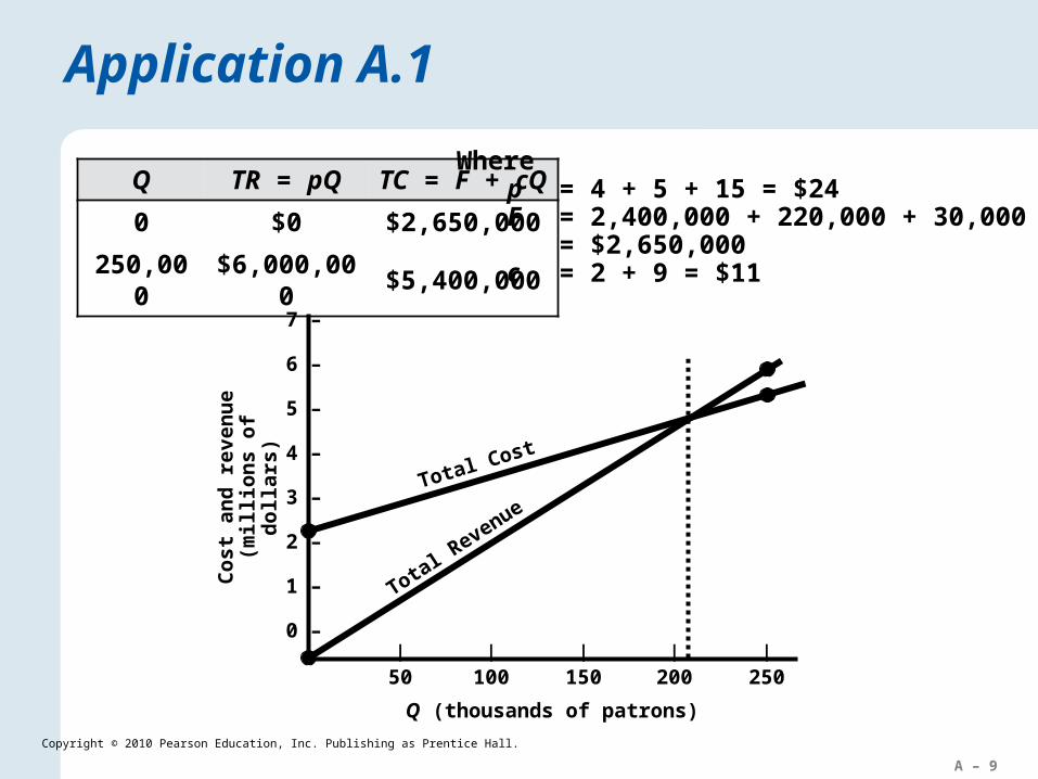
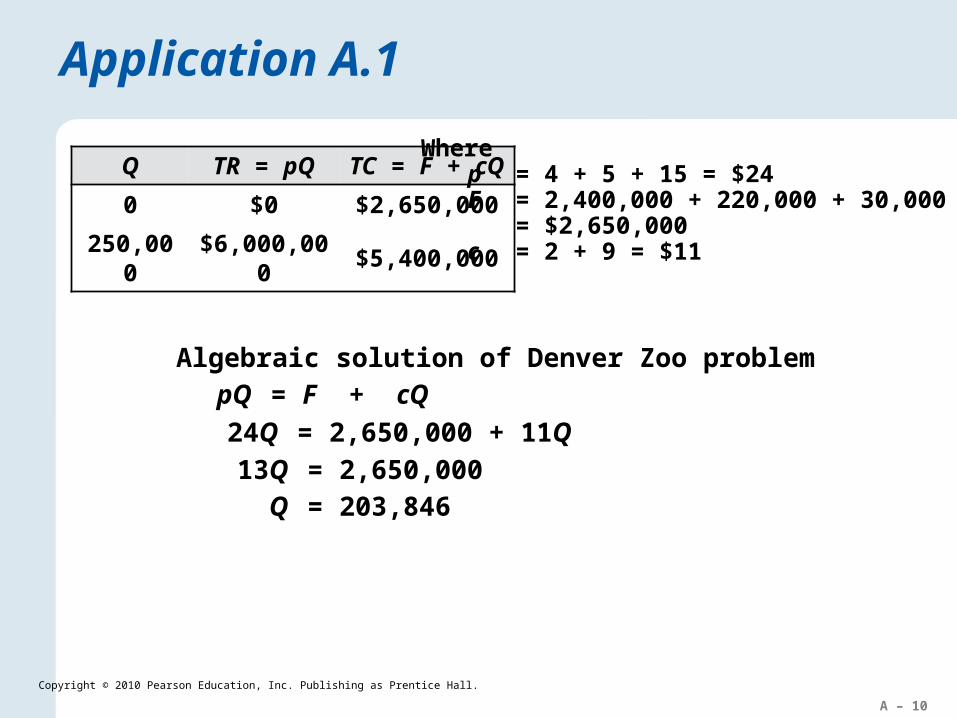
Q TR = pQ TC = F + cQ
0 $0 $2,650,000
250,000 $6,000,000 $5,400,000
7 –
6 –
5 –
4 –
3 –
2 –
1 –
0 –| | | | | |
50 100 150 200 250
Co
st a
nd
rev
enu
e (m
illi
on
s o
f d
oll
ars)
Q (thousands of patrons)
Total Cost
Total Revenue
Wherep = 4 + 5 + 15 = $24F = 2,400,000 + 220,000 + 30,000
= $2,650,000c = 2 + 9 = $11
A – 10
Copyright © 2010 Pearson Education, Inc. Publishing as Prentice Hall.
Application A.1
Q TR = pQ TC = F + cQ
0 $0 $2,650,000
250,000 $6,000,000 $5,400,000
Wherep = 4 + 5 + 15 = $24F = 2,400,000 + 220,000 + 30,000
= $2,650,000c = 2 + 9 = $11
Algebraic solution of Denver Zoo problempQ = F + cQ
24Q = 2,650,000 + 11Q
13Q = 2,650,000Q = 203,846
A – 11
Copyright © 2010 Pearson Education, Inc. Publishing as Prentice Hall.
Sensitivity Analysis
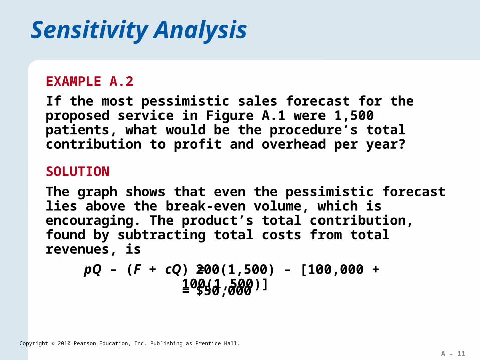
EXAMPLE A.2
If the most pessimistic sales forecast for the proposed service in Figure A.1 were 1,500 patients, what would be the procedure’s total contribution to profit and overhead per year?
SOLUTION
The graph shows that even the pessimistic forecast lies above the break-even volume, which is encouraging. The product’s total contribution, found by subtracting total costs from total revenues, is
200(1,500) – [100,000 + 100(1,500)]
pQ – (F + cQ) =
= $50,000
A – 12
Copyright © 2010 Pearson Education, Inc. Publishing as Prentice Hall.
Evaluating Processes
Choices must be made between two processes or between an internal process and buying services or materials on the outside
We assume that the decision does not affect revenues
The analyst finds the quantity for which the total costs for two alternatives are equal
A – 13
Copyright © 2010 Pearson Education, Inc. Publishing as Prentice Hall.
Evaluating Processes
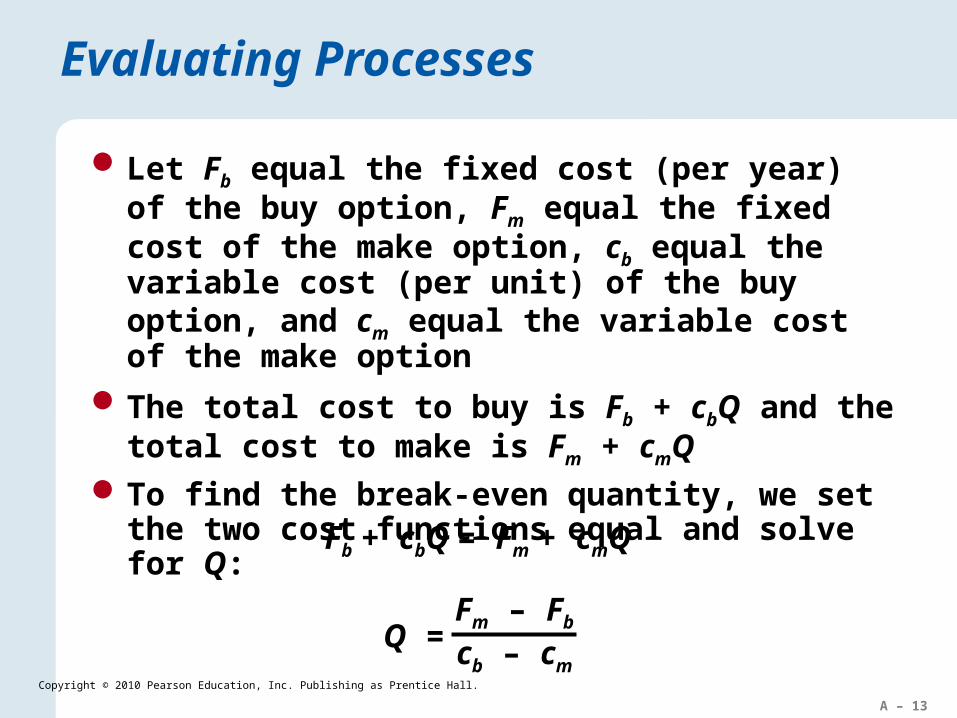
Let Fb equal the fixed cost (per year) of the buy option, Fm equal the fixed cost of the make option, cb equal the variable cost (per unit) of the buy option, and cm equal the variable cost of the make option
The total cost to buy is Fb + cbQ and the total cost to make is Fm + cmQ
To find the break-even quantity, we set the two cost functions equal and solve for Q:
Fb + cbQ = Fm + cmQ
Q =Fm – Fb
cb – cm
A – 14
Copyright © 2010 Pearson Education, Inc. Publishing as Prentice Hall.
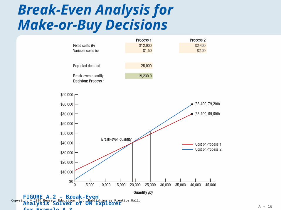
Break-Even Analysis for Make-or-Buy Decisions
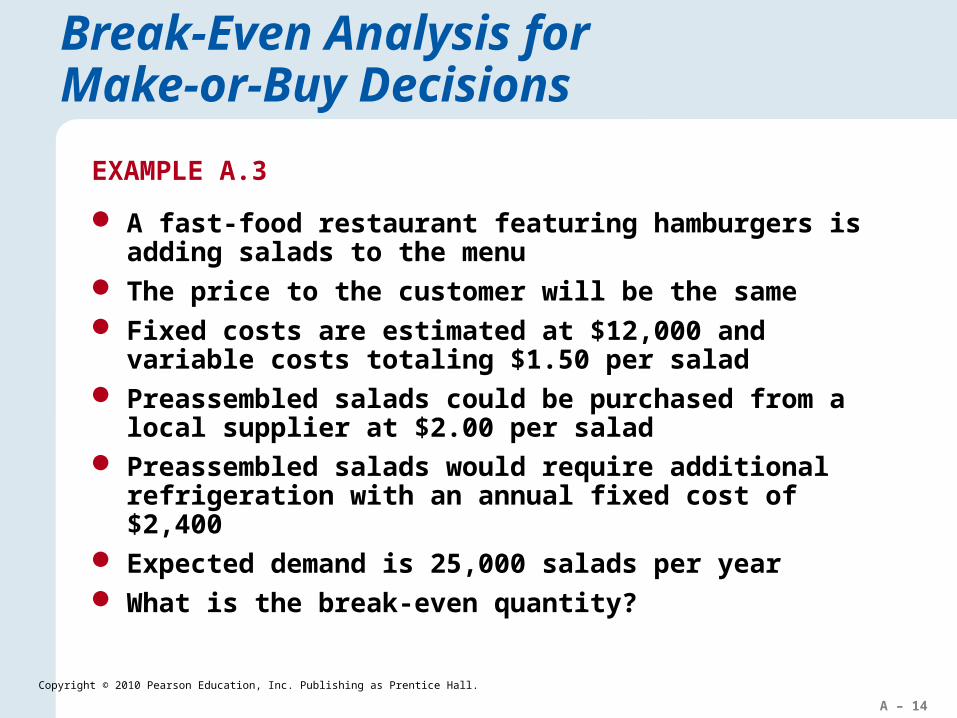
A fast-food restaurant featuring hamburgers is adding salads to the menu
The price to the customer will be the same Fixed costs are estimated at $12,000 and variable costs
totaling $1.50 per salad Preassembled salads could be purchased from a local
supplier at $2.00 per salad Preassembled salads would require additional refrigeration
with an annual fixed cost of $2,400 Expected demand is 25,000 salads per year What is the break-even quantity?
EXAMPLE A.3
A – 15
Copyright © 2010 Pearson Education, Inc. Publishing as Prentice Hall.
Break-Even Analysis for Make-or-Buy Decisions
SOLUTION
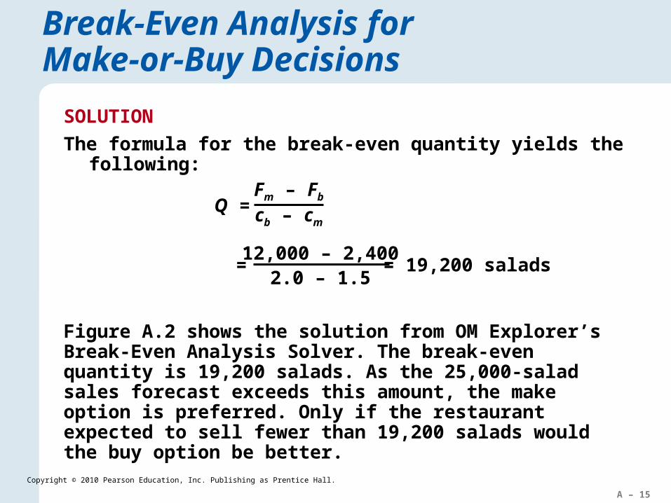
The formula for the break-even quantity yields the following:
Q =Fm – Fb
cb – cm
= 19,200 salads=12,000 – 2,400
2.0 – 1.5
Figure A.2 shows the solution from OM Explorer’s Break-Even Analysis Solver. The break-even quantity is 19,200 salads. As the 25,000-salad sales forecast exceeds this amount, the make option is preferred. Only if the restaurant expected to sell fewer than 19,200 salads would the buy option be better.
A – 16
Copyright © 2010 Pearson Education, Inc. Publishing as Prentice Hall.
Break-Even Analysis for Make-or-Buy Decisions
FIGURE A.2 – Break-Even Analysis Solver of OM Explorer for Example A.3
A – 17
Copyright © 2010 Pearson Education, Inc. Publishing as Prentice Hall.
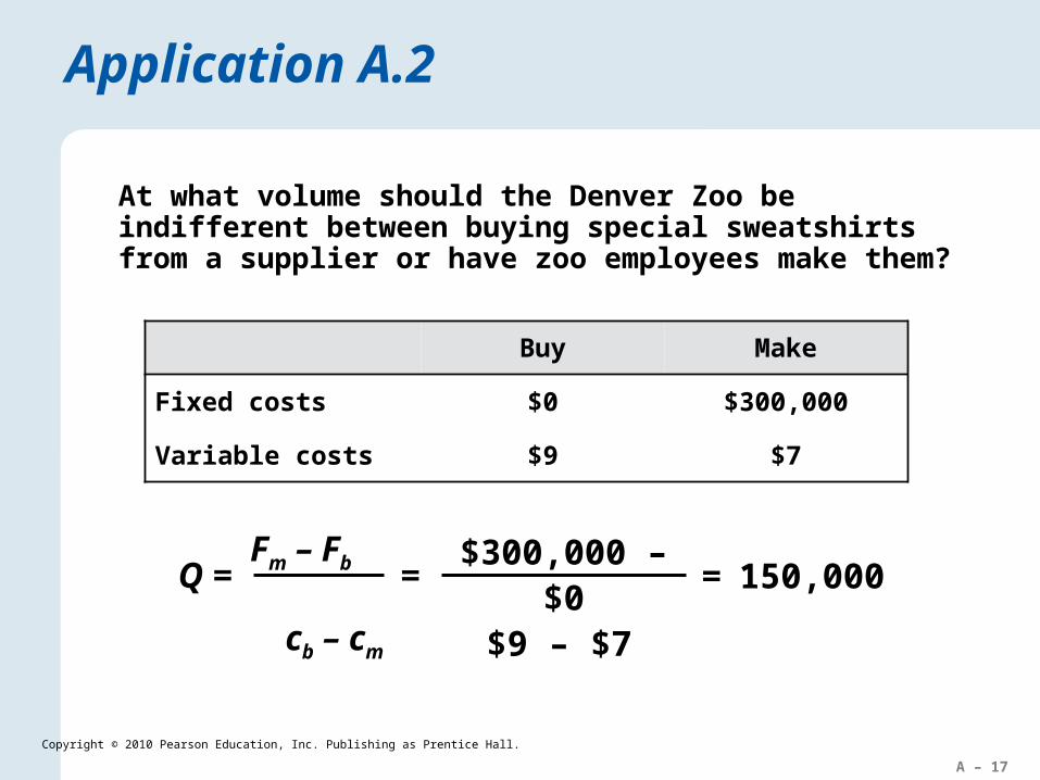
Application A.2
Fm – Fb cb –
cm
Q = = 150,000
At what volume should the Denver Zoo be indifferent between buying special sweatshirts from a supplier or have zoo employees make them?
=$300,000 – $0
$9 – $7
Buy Make
Fixed costs $0 $300,000
Variable costs $9 $7
A – 18
Copyright © 2010 Pearson Education, Inc. Publishing as Prentice Hall.
Preference Matrix
A Preference Matrix is a table that allows you to rate an alternative according to several performance criteria
The criteria can be scored on any scale as long as the same scale is applied to all the alternatives being compared
Each score is weighted according to its perceived importance, with the total weights typically equaling 100
The total score is the sum of the weighted scores (weight × score) for all the criteria and compared against scores for alternatives
A – 19
Copyright © 2010 Pearson Education, Inc. Publishing as Prentice Hall.
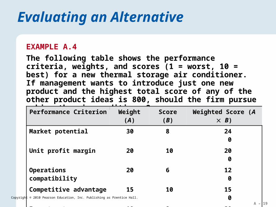
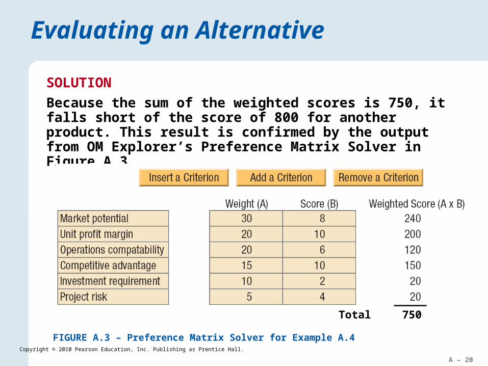
EXAMPLE A.4
The following table shows the performance criteria, weights, and scores (1 = worst, 10 = best) for a new thermal storage air conditioner. If management wants to introduce just one new product and the highest total score of any of the other product ideas is 800, should the firm pursue making the air conditioner?
Evaluating an Alternative
Performance Criterion Weight (A) Score (B) Weighted Score (A B)
Market potential30
8 240
Unit profit margin20 10
200
Operations compatibility20
6 120
Competitive advantage15 10
150
Investment requirements10
2 20
Project risk 5 4 20
Weighted score = 750
A – 20
Copyright © 2010 Pearson Education, Inc. Publishing as Prentice Hall.
SOLUTION
Because the sum of the weighted scores is 750, it falls short of the score of 800 for another product. This result is confirmed by the output from OM Explorer’s Preference Matrix Solver in Figure A.3.
Evaluating an Alternative
FIGURE A.3 – Preference Matrix Solver for Example A.4
Total 750
A – 21
Copyright © 2010 Pearson Education, Inc. Publishing as Prentice Hall.
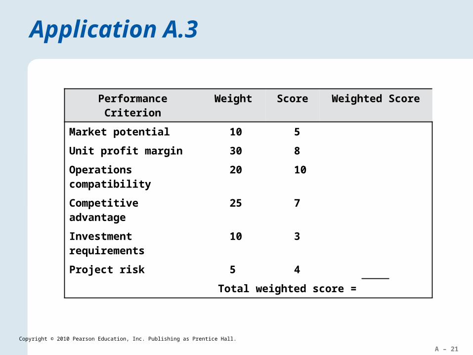
Application A.3
Performance Criterion Weight Score Weighted Score
Market potential10 5
Unit profit margin30 8
Operations compatibility20 10
Competitive advantage25 7
Investment requirements10 3
Project risk 54
Total weighted score =
A – 22
Copyright © 2010 Pearson Education, Inc. Publishing as Prentice Hall.
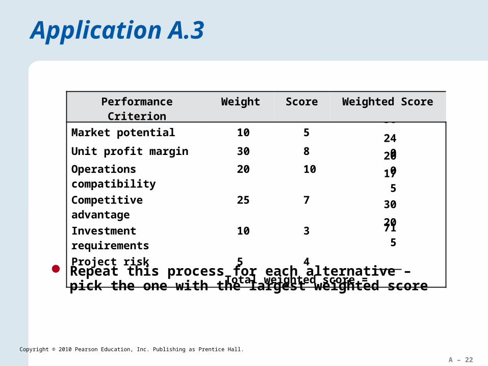
Application A.3
Repeat this process for each alternative – pick the one with the largest weighted score
50
200
240
175
30
20
715
Performance Criterion Weight Score Weighted Score
Market potential10 5
Unit profit margin30 8
Operations compatibility20 10
Competitive advantage25 7
Investment requirements10 3
Project risk 54
Total weighted score =
A – 23
Copyright © 2010 Pearson Education, Inc. Publishing as Prentice Hall.
Criticisms
Requires the manager to state criterion weights before examining alternatives, but they may not know in advance what is important and what is not
Allows one very low score to be overridden by high scores on other factors
May cause managers to ignore important signals
A – 24
Copyright © 2010 Pearson Education, Inc. Publishing as Prentice Hall.
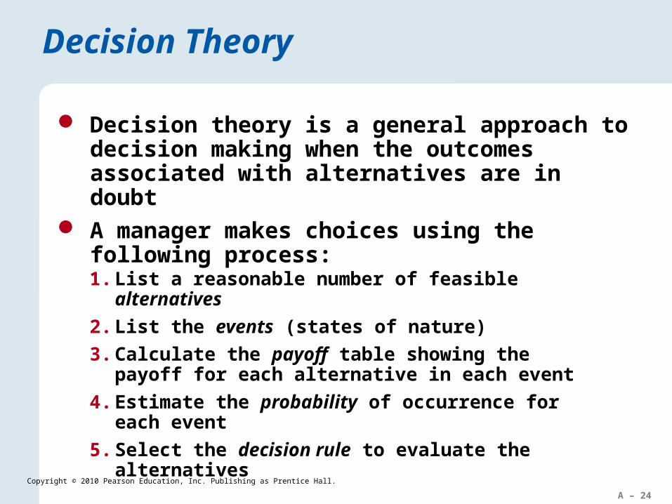
Decision theory is a general approach to decision making when the outcomes associated with alternatives are in doubt
A manager makes choices using the following process:
Decision Theory
1. List a reasonable number of feasible alternatives
2. List the events (states of nature)
3. Calculate the payoff table showing the payoff for each alternative in each event
4. Estimate the probability of occurrence for each event
5. Select the decision rule to evaluate the alternatives
A – 25
Copyright © 2010 Pearson Education, Inc. Publishing as Prentice Hall.
Decision Making Under Certainty
The simplest solution is when the manager knows which event will occur
Here the decision rule is to pick the alternative with the best payoff for the known event
A – 26
Copyright © 2010 Pearson Education, Inc. Publishing as Prentice Hall.
Decisions Under Certainty
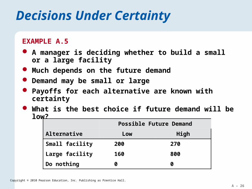
EXAMPLE A.5
A manager is deciding whether to build a small or a large facility
Much depends on the future demand Demand may be small or large Payoffs for each alternative are known with certainty What is the best choice if future demand will be low?
Possible Future Demand
Alternative Low High
Small facility 200 270
Large facility 160 800
Do nothing 0 0
A – 27
Copyright © 2010 Pearson Education, Inc. Publishing as Prentice Hall.
Decisions Under Certainty
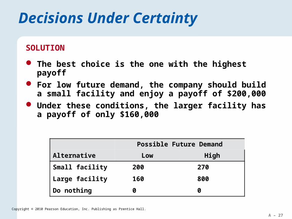
SOLUTION
The best choice is the one with the highest payoff For low future demand, the company should build a small
facility and enjoy a payoff of $200,000 Under these conditions, the larger facility has a payoff of
only $160,000
Possible Future Demand
Alternative Low High
Small facility 200 270
Large facility 160 800
Do nothing 0 0
A – 28
Copyright © 2010 Pearson Education, Inc. Publishing as Prentice Hall.
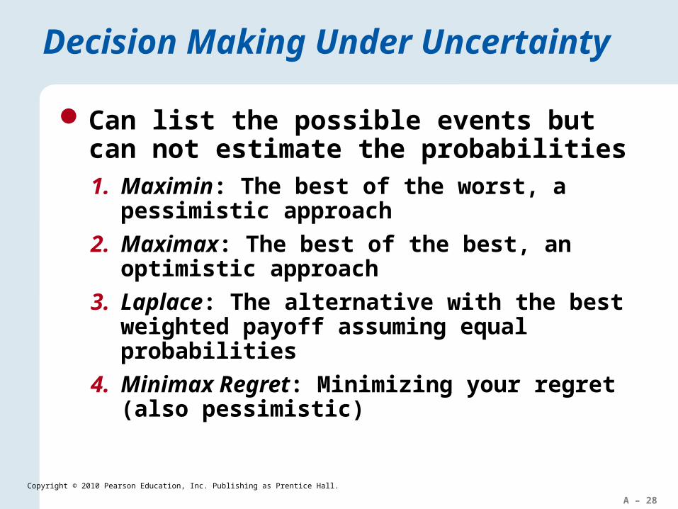
Can list the possible events but can not estimate the probabilities
Decision Making Under Uncertainty
1. Maximin: The best of the worst, a pessimistic approach
2. Maximax: The best of the best, an optimistic approach
3. Laplace: The alternative with the best weighted payoff assuming equal probabilities
4. Minimax Regret: Minimizing your regret (also pessimistic)
A – 29
Copyright © 2010 Pearson Education, Inc. Publishing as Prentice Hall.
Decisions Under Uncertainty
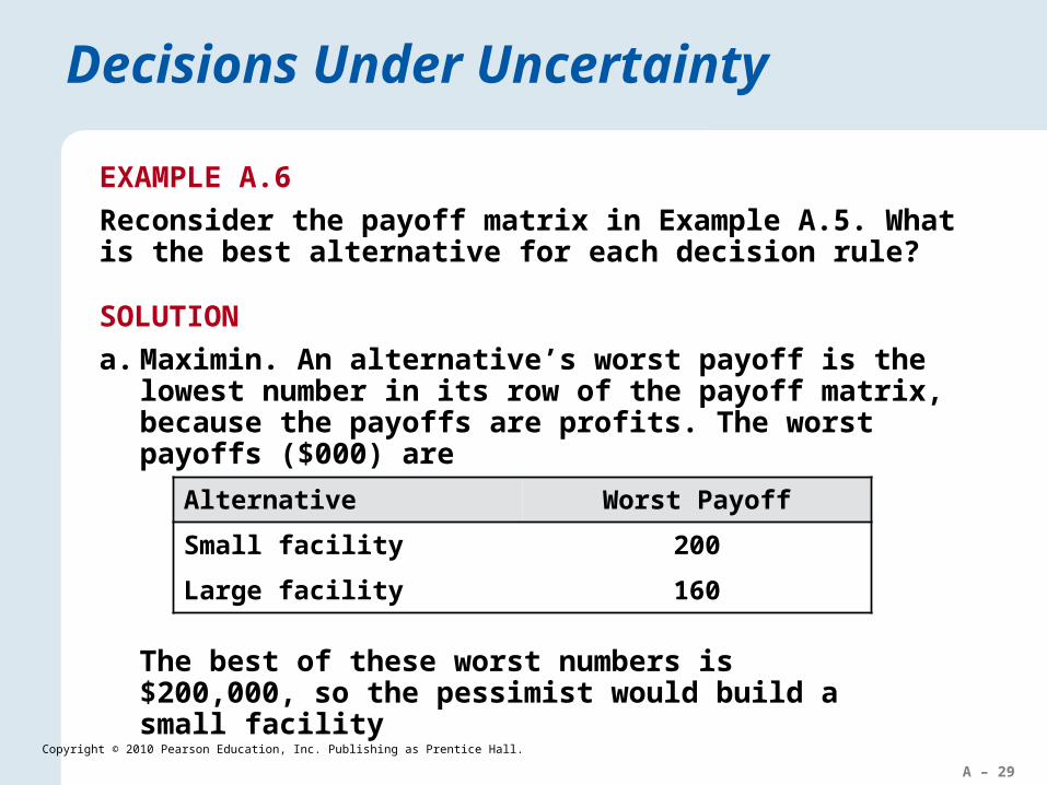
EXAMPLE A.6
Reconsider the payoff matrix in Example A.5. What is the best alternative for each decision rule?
SOLUTION
a. Maximin. An alternative’s worst payoff is the lowest number in its row of the payoff matrix, because the payoffs are profits. The worst payoffs ($000) are
Alternative Worst Payoff
Small facility 200
Large facility 160
The best of these worst numbers is $200,000, so the pessimist would build a small facility
A – 30
Copyright © 2010 Pearson Education, Inc. Publishing as Prentice Hall.
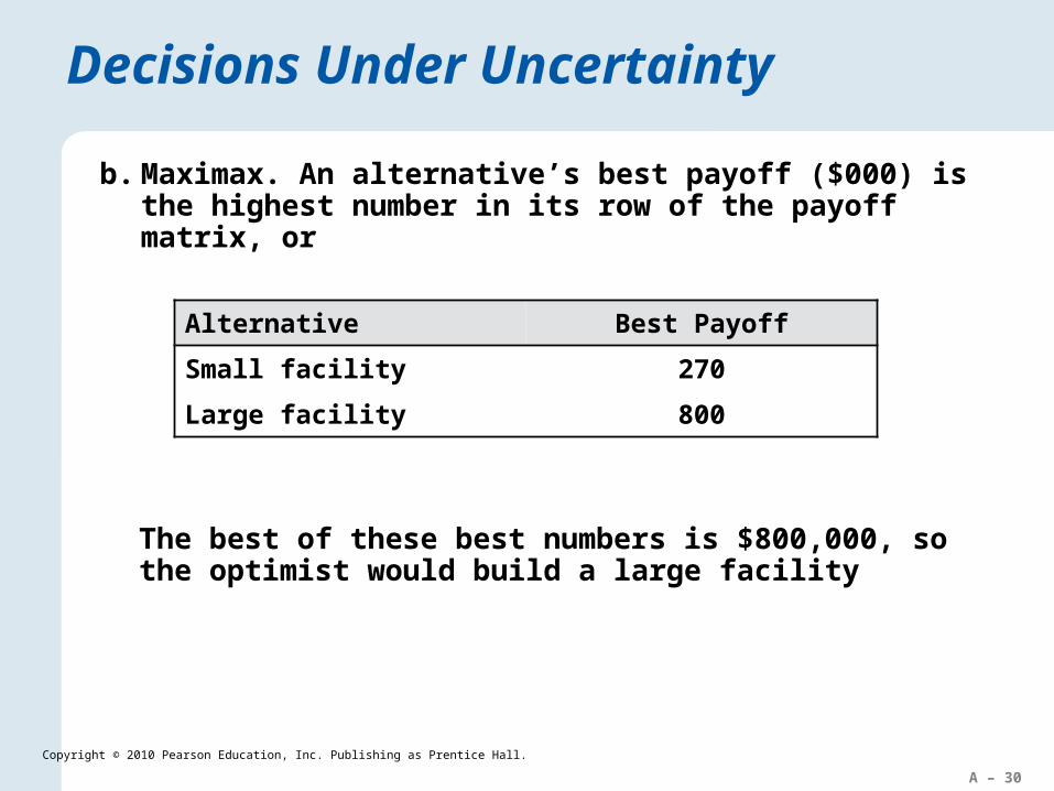
Decisions Under Uncertainty
b. Maximax. An alternative’s best payoff ($000) is the highest number in its row of the payoff matrix, or
Alternative Best Payoff
Small facility 270
Large facility 800
The best of these best numbers is $800,000, so the optimist would build a large facility
A – 31
Copyright © 2010 Pearson Education, Inc. Publishing as Prentice Hall.
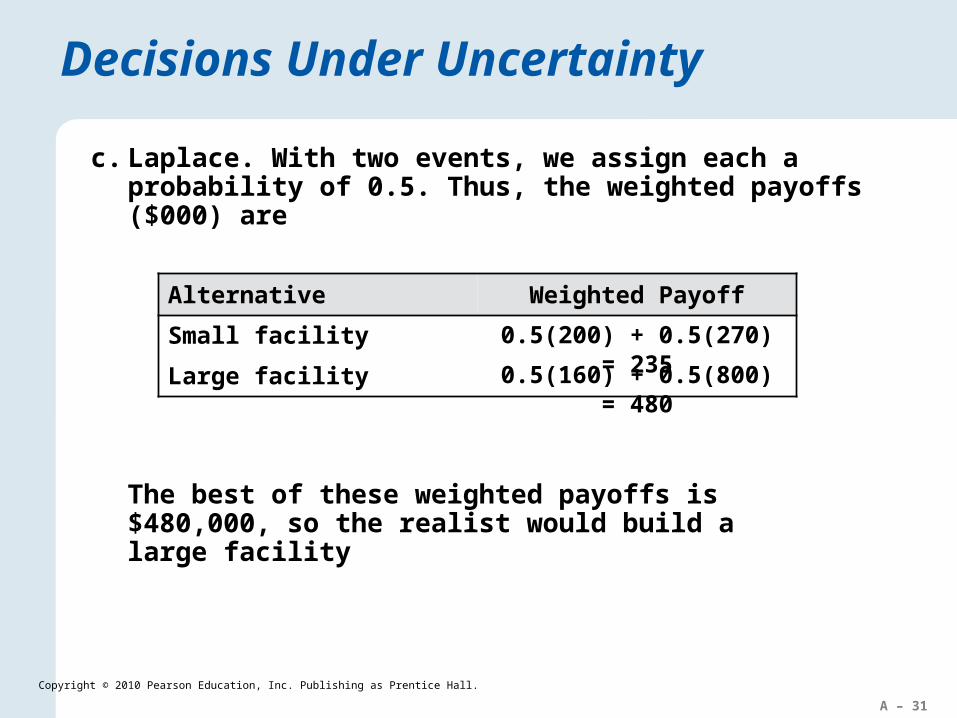
Decisions Under Uncertainty
c. Laplace. With two events, we assign each a probability of 0.5. Thus, the weighted payoffs ($000) are
The best of these weighted payoffs is $480,000, so the realist would build a large facility
0.5(200) + 0.5(270) = 235
0.5(160) + 0.5(800) = 480
Alternative Weighted Payoff
Small facility
Large facility
A – 32
Copyright © 2010 Pearson Education, Inc. Publishing as Prentice Hall.
Decisions Under Uncertainty
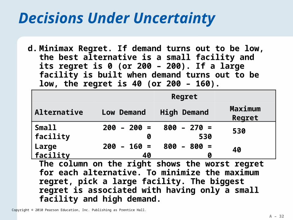
d. Minimax Regret. If demand turns out to be low, the best alternative is a small facility and its regret is 0 (or 200 – 200). If a large facility is built when demand turns out to be low, the regret is 40 (or 200 – 160).
Regret
Alternative Low Demand High Demand Maximum Regret
Small facility 200 – 200 = 0 800 – 270 = 530 530
Large facility 200 – 160 = 40 800 – 800 = 0 40
The column on the right shows the worst regret for each alternative. To minimize the maximum regret, pick a large facility. The biggest regret is associated with having only a small facility and high demand.
A – 33
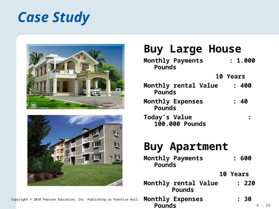
Case Study
Buy Large HouseMonthly Payments : 1.000 Pounds
10 Years
Monthly rental Value : 400 Pounds
Monthly Expenses : 40 Pounds
Today’s Value : 100.000 Pounds
Buy ApartmentMonthly Payments : 600 Pounds
10 Years
Monthly rental Value : 220 Pounds
Monthly Expenses : 30 Pounds
Today’s Value : 60.000 Pounds
Copyright © 2010 Pearson Education, Inc. Publishing as Prentice Hall.
A – 34
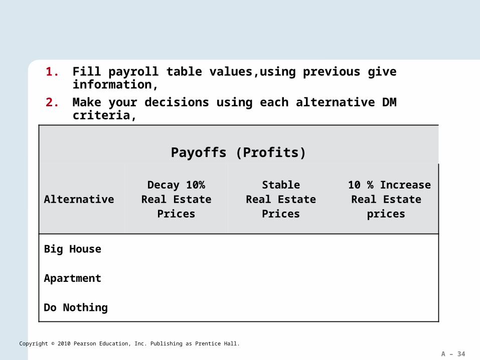
1. Fill payroll table values,using previous give information,
2. Make your decisions using each alternative DM criteria,
3. Make your final decision and interprete it.
Copyright © 2010 Pearson Education, Inc. Publishing as Prentice Hall.
Payoffs (Profits)
Alternative Decay 10%Real Estate Prices
StableReal Estate Prices
10 % IncreaseReal Estate prices
Big House
Apartment
Do Nothing
A – 35
Copyright © 2010 Pearson Education, Inc. Publishing as Prentice Hall.
A – 36
Copyright © 2010 Pearson Education, Inc. Publishing as Prentice Hall.
Application A.4
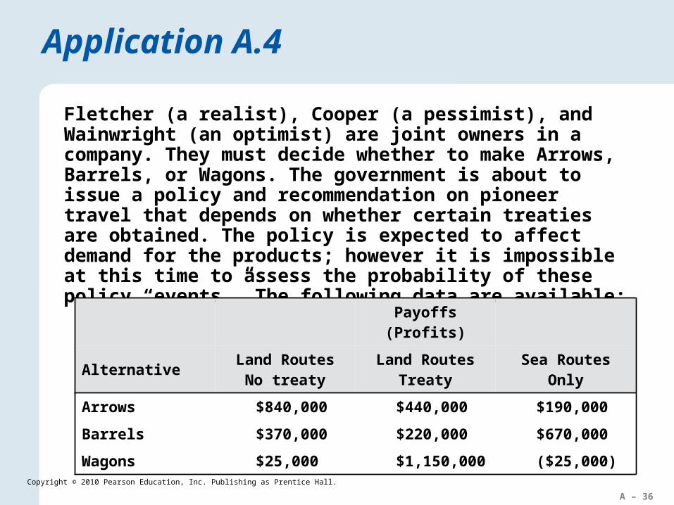
Fletcher (a realist), Cooper (a pessimist), and Wainwright (an optimist) are joint owners in a company. They must decide whether to make Arrows, Barrels, or Wagons. The government is about to issue a policy and recommendation on pioneer travel that depends on whether certain treaties are obtained. The policy is expected to affect demand for the products; however it is impossible at this time to assess the probability of these policy “events.” The following data are available:
Payoffs (Profits)
Alternative Land RoutesNo treaty
Land RoutesTreaty
Sea RoutesOnly
Arrows $840,000 $440,000 $190,000
Barrels $370,000 $220,000 $670,000
Wagons $25,000 $1,150,000 ($25,000)

A – 37
Copyright © 2010 Pearson Education, Inc. Publishing as Prentice Hall.
Application A.4
Fletcher (a realist), Cooper (a pessimist), and Wainwright (an optimist) are joint owners in a company. They must decide whether to make Arrows, Barrels, or Wagons. The government is about to issue a policy and recommendation on pioneer travel that depends on whether certain treaties are obtained. The policy is expected to affect demand for the products; however it is impossible at this time to assess the probability of these policy “events.” The following data are available:
Payoffs (Profits)
Alternative Land RoutesNo treaty
Land RoutesTreaty
Sea RoutesOnly
Arrows $840,000 $440,000 $190,000
Barrels $370,000 $220,000 $670,000
Wagons $25,000 $1,150,000 ($25,000)
A – 38
Copyright © 2010 Pearson Education, Inc. Publishing as Prentice Hall.
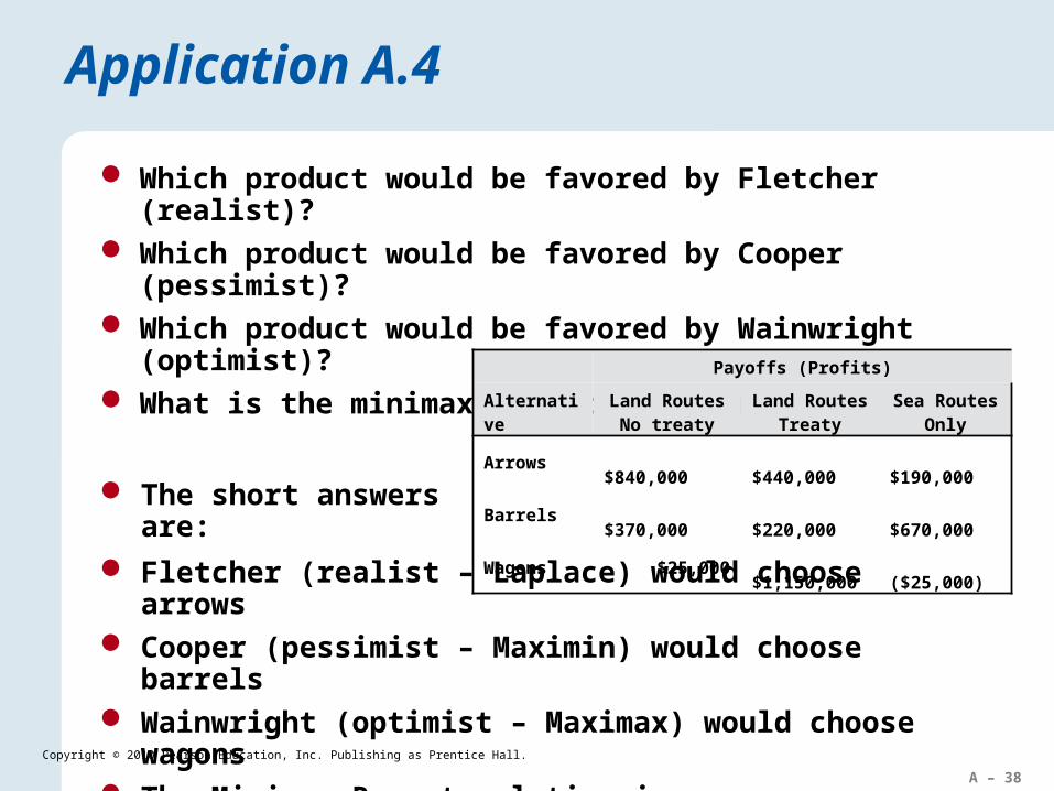
Application A.4
Which product would be favored by Fletcher (realist)? Which product would be favored by Cooper (pessimist)? Which product would be favored by Wainwright (optimist)? What is the minimax regret solution?
The short answers are:
Payoffs (Profits)
AlternativeLand Routes
No treatyLand Routes
TreatySea Routes
Only
Arrows$840,000 $440,000 $190,000
Barrels$370,000 $220,000 $670,000
Wagons$25,000 $1,150,000 ($25,000) Fletcher (realist – Laplace) would choose arrows
Cooper (pessimist – Maximin) would choose barrels Wainwright (optimist – Maximax) would choose wagons The Minimax Regret solution is arrows
A – 39
Copyright © 2010 Pearson Education, Inc. Publishing as Prentice Hall.
Decisions Under Risk
The manager can list the possible events and estimate their probabilities
The manager has less information than decision making under certainty, but more information than with decision making under uncertainty
The expected value rule is widely usedThis rule is similar to the Laplace decision
rule, except that the events are no longer assumed to be equally likely
A – 40
Copyright © 2010 Pearson Education, Inc. Publishing as Prentice Hall.
Decisions Under Risk
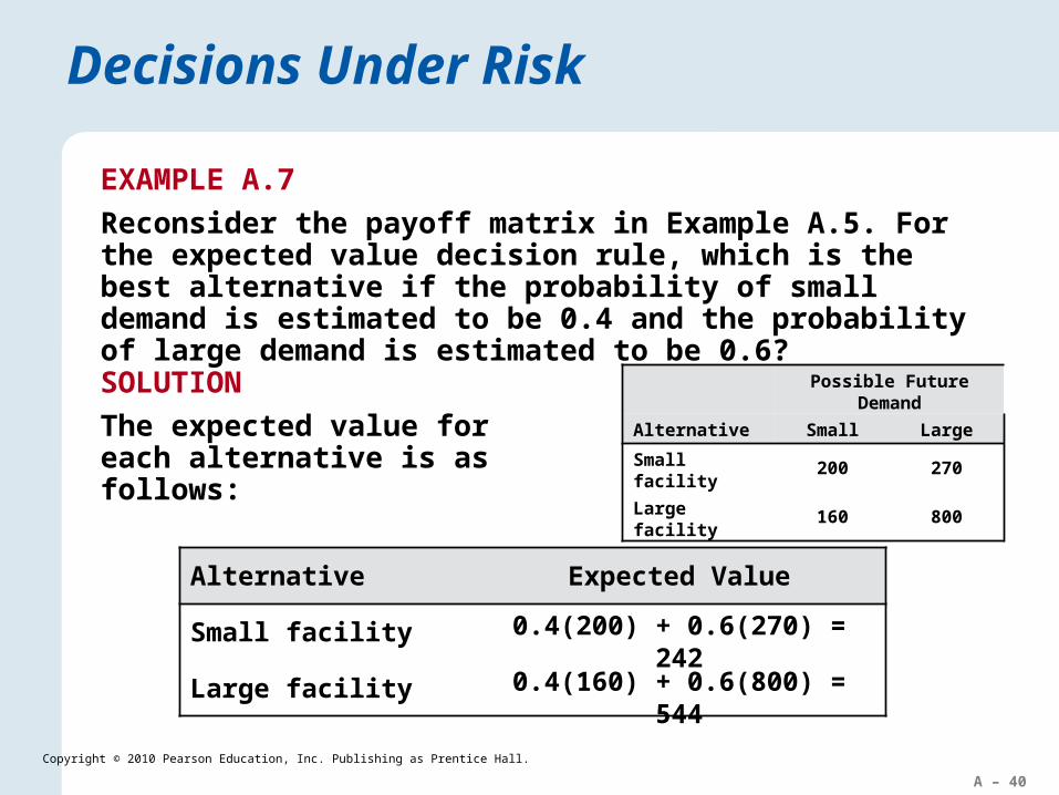
EXAMPLE A.7
Reconsider the payoff matrix in Example A.5. For the expected value decision rule, which is the best alternative if the probability of small demand is estimated to be 0.4 and the probability of large demand is estimated to be 0.6?
SOLUTION
The expected value for each alternative is as follows:
Possible Future Demand
Alternative Small Large
Small facility 200 270
Large facility 160 800
0.4(200) + 0.6(270) = 242
0.4(160) + 0.6(800) = 544
Alternative Expected Value
Small facility
Large facility
A – 41
Copyright © 2010 Pearson Education, Inc. Publishing as Prentice Hall.
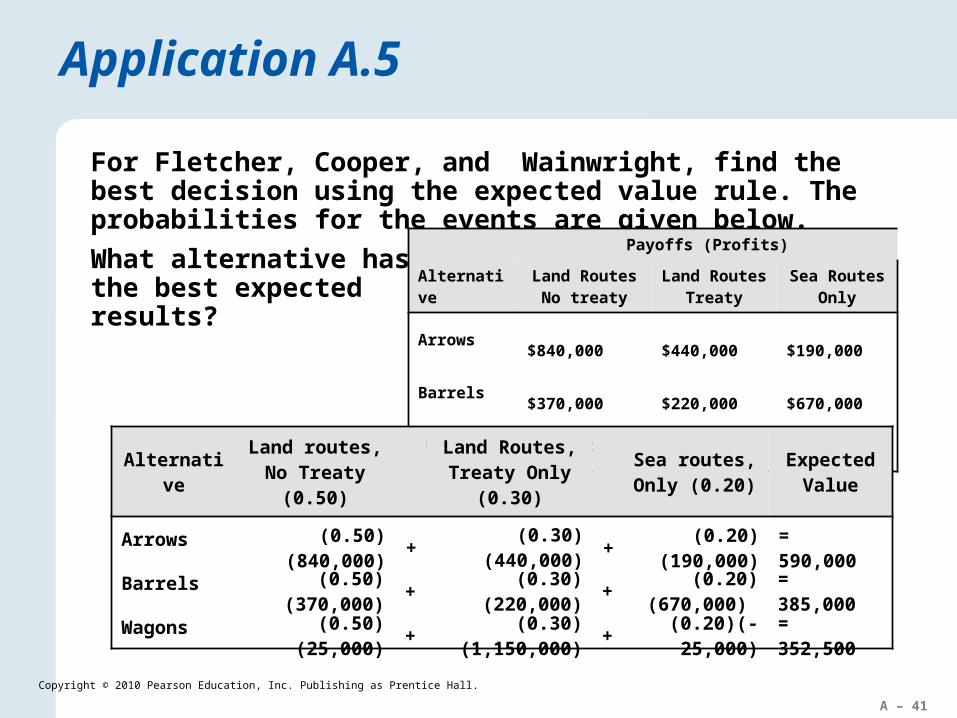
Application A.5
For Fletcher, Cooper, and Wainwright, find the best decision using the expected value rule. The probabilities for the events are given below.
What alternative has the best expected results?
Payoffs (Profits)
AlternativeLand Routes
No treatyLand Routes
TreatySea Routes
Only
Arrows$840,000 $440,000 $190,000
Barrels$370,000 $220,000 $670,000
Wagons$25,000 $1,150,000 ($25,000)
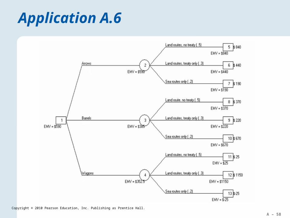
(0.50)(840,000) + (0.30)(440,000) +(0.20)
(190,000)= 590,000
(0.50)(370,000) + (0.30)(220,000) + (0.20)(670,000)
= 385,000
(0.50)(25,000) + (0.30)(1,150,000) + (0.20)(-25,000) = 352,500
AlternativeLand routes,
No Treaty(0.50)
Land Routes, Treaty Only
(0.30)
Sea routes, Only (0.20)
Expected Value
Arrows
Barrels
Wagons
A – 42
Copyright © 2010 Pearson Education, Inc. Publishing as Prentice Hall.
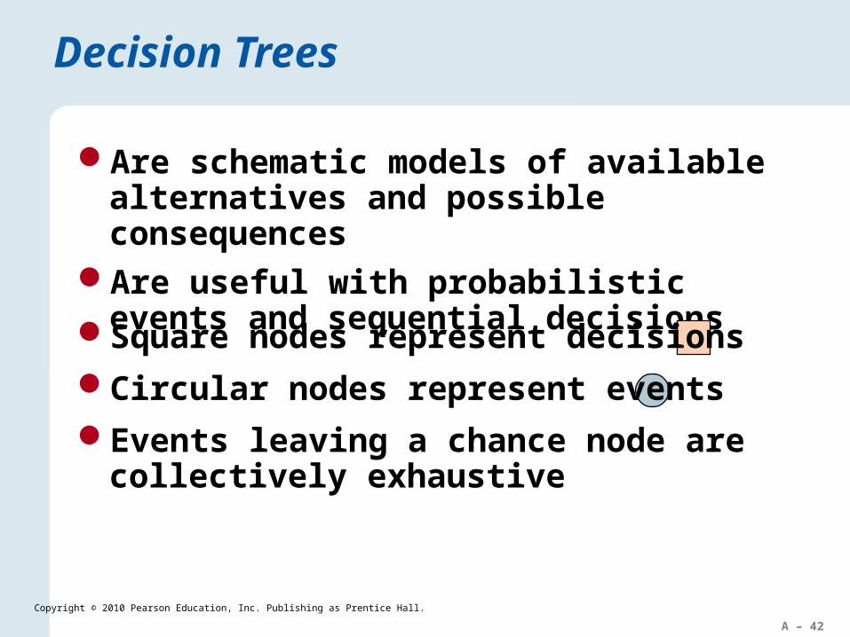
Are schematic models of available alternatives and possible consequences
Are useful with probabilistic events and sequential decisions
Decision Trees
Square nodes represent decisions
Circular nodes represent events
Events leaving a chance node are collectively exhaustive
A – 43
Copyright © 2010 Pearson Education, Inc. Publishing as Prentice Hall.
Conditional payoffs for each possible alternative-event combination shown at the end of each combination
Draw the decision tree from left to rightCalculate expected payoff to solve the
decision tree from right to left
Decision Trees
A – 44
Copyright © 2010 Pearson Education, Inc. Publishing as Prentice Hall.
Payoff 1
Payoff 2
Payoff 3
Alternative 3
Alternative 4
Alternative 5
Payoff 1
Payoff 2
Payoff 3
E1 & Probability
E2 & Probability
E3 & Probability
Altern
ativ
e 1
Alternative 2
E2 & Probability
E3 & Probability
E 1 &
Pro
babili
ty
Payoff 1
Payoff 2
1stdecision
1
Possible2nd decision
2
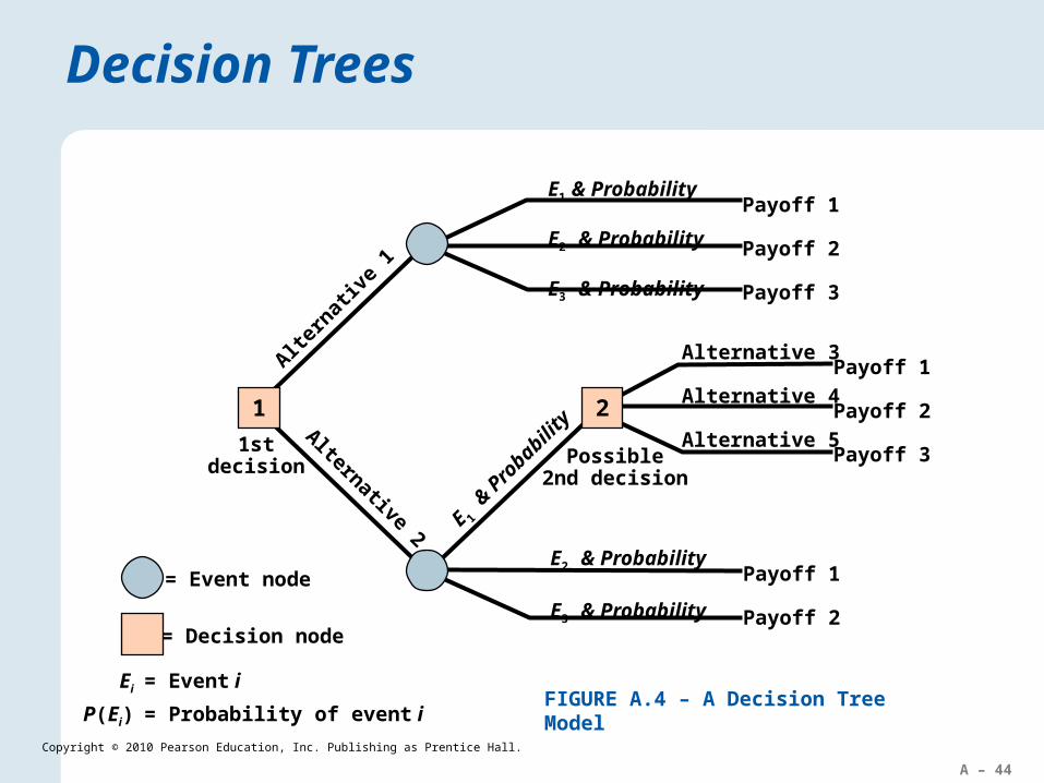
Decision Trees
= Event node
= Decision node
Ei = Event i
P(Ei) = Probability of event iFIGURE A.4 – A Decision Tree Model
A – 45
Copyright © 2010 Pearson Education, Inc. Publishing as Prentice Hall.
Decision Trees
After drawing a decision tree, we solve it by working from right to left, calculating the expected payoff for each of its possible paths
1. For an event node, we multiply the payoff of each event branch by the event’s probability and add these products to get the event node’s expected payoff
2. For a decision node, we pick the alternative that has the best expected payoff
A – 46
Copyright © 2010 Pearson Education, Inc. Publishing as Prentice Hall.
Decision Trees
Various software is available for drawing and/or analyzing decision trees, including PowerPoint can be used to draw decision
trees, but does not have the capability to analyze the decision tree
POM with Windows SmartDraw PrecisionTree decision analysis from Palisade
Corporation
TreePlan
A – 47
Copyright © 2010 Pearson Education, Inc. Publishing as Prentice Hall.
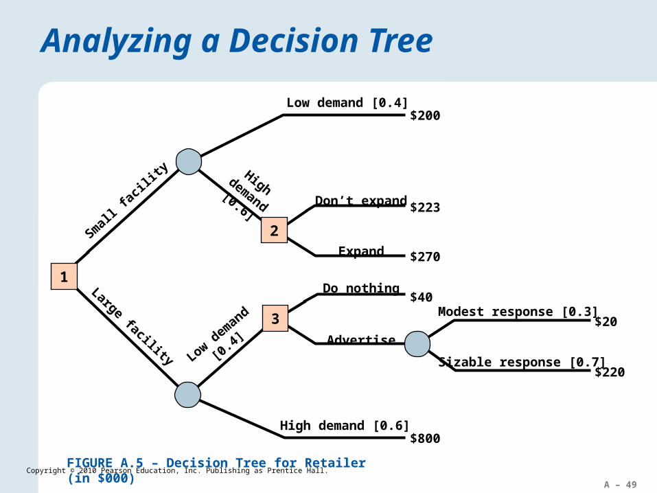
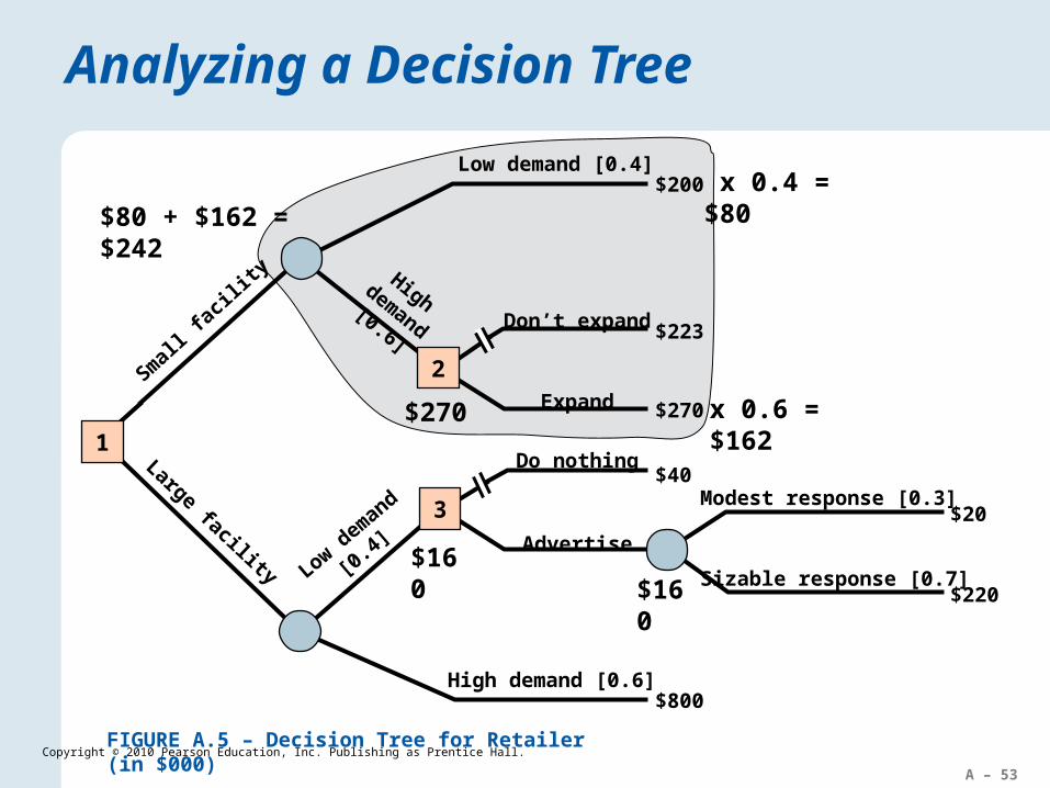
Analyzing a Decision Tree
EXAMPLE A.8
A retailer will build a small or a large facility at a new location Demand can be either small or large, with probabilities
estimated to be 0.4 and 0.6, respectively For a small facility and high demand, not expanding will have
a payoff of $223,000 and a payoff of $270,000 with expansion For a small facility and low demand the payoff is $200,000 For a large facility and low demand, doing nothing has a
payoff of $40,000 The response to advertising may be either modest or sizable,
with their probabilities estimated to be 0.3 and 0.7, respectively
For a modest response the payoff is $20,000 and $220,000 if the response is sizable
For a large facility and high demand the payoff is $800,000
A – 48
Copyright © 2010 Pearson Education, Inc. Publishing as Prentice Hall.
Analyzing a Decision Tree
SOLUTION
The decision tree in Figure A.5 shows the event probability and the payoff for each of the seven alternative-event combinations. The first decision is whether to build a small or a large facility. Its node is shown first, to the left, because it is the decision the retailer must make now. The second decision node is reached only if a small facility is built and demand turns out to be high. Finally, the third decision point is reached only if the retailer builds a large facility and demand turns out to be low.
A – 49
Copyright © 2010 Pearson Education, Inc. Publishing as Prentice Hall.
Analyzing a Decision Tree
$200
$223
$270
$40
$800
$20
$220
Don’t expand
Expand
Low demand [0.4]
High demand
[0.6]
2
FIGURE A.5 – Decision Tree for Retailer (in $000)
Low dem
and
[0.4]
High demand [0.6]
3
Do nothing
Advertise
Modest response [0.3]
Sizable response [0.7]
Smal
l fac
ility
Large facility
1
A – 50
Copyright © 2010 Pearson Education, Inc. Publishing as Prentice Hall.
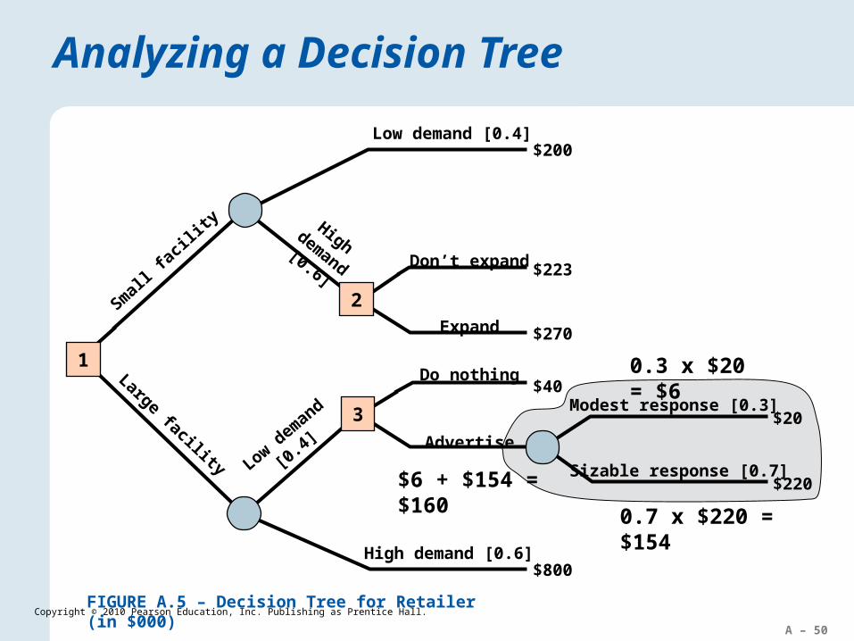
Analyzing a Decision Tree
$200
$223
$270
$40
$800
$20
$220
Don’t expand
Expand
Low demand [0.4]
High demand
[0.6]
2
FIGURE A.5 – Decision Tree for Retailer (in $000)
Low dem
and
[0.4]
High demand [0.6]
3
Do nothing
Advertise
Modest response [0.3]
Sizable response [0.7]
Smal
l fac
ility
Large facility
1 0.3 x $20 = $6
0.7 x $220 = $154
$6 + $154 = $160
A – 51
Copyright © 2010 Pearson Education, Inc. Publishing as Prentice Hall.
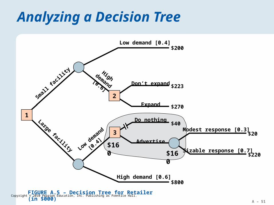
Analyzing a Decision Tree
$200
$223
$270
$40
$800
$20
$220
Don’t expand
Expand
Low demand [0.4]
High demand
[0.6]
2
FIGURE A.5 – Decision Tree for Retailer (in $000)
Low dem
and
[0.4]
High demand [0.6]
3
Do nothing
Advertise
Modest response [0.3]
Sizable response [0.7]
Smal
l fac
ility
Large facility
1
$160$160
A – 52
Copyright © 2010 Pearson Education, Inc. Publishing as Prentice Hall.
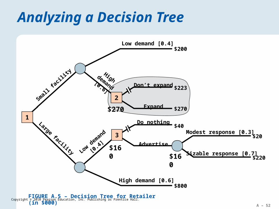
Analyzing a Decision Tree
$200
$223
$270
$40
$800
$20
$220
Don’t expand
Expand
Low demand [0.4]
High demand
[0.6]
2
FIGURE A.5 – Decision Tree for Retailer (in $000)
Low dem
and
[0.4]
High demand [0.6]
3
Do nothing
Advertise
Modest response [0.3]
Sizable response [0.7]
Smal
l fac
ility
Large facility
1
$160$160
$270
A – 53
Copyright © 2010 Pearson Education, Inc. Publishing as Prentice Hall.
Analyzing a Decision Tree
$200
$223
$270
$40
$800
$20
$220
Don’t expand
Expand
Low demand [0.4]
High demand
[0.6]
2
FIGURE A.5 – Decision Tree for Retailer (in $000)
Low dem
and
[0.4]
High demand [0.6]
3
Do nothing
Advertise
Modest response [0.3]
Sizable response [0.7]
Smal
l fac
ility
Large facility
1
$160$160
$270
x 0.4 = $80
x 0.6 = $162
$80 + $162 = $242
A – 54
Copyright © 2010 Pearson Education, Inc. Publishing as Prentice Hall.
Analyzing a Decision Tree
$200
$223
$270
$40
$800
$20
$220
Don’t expand
Expand
Low demand [0.4]
High demand
[0.6]
2
FIGURE A.5 – Decision Tree for Retailer (in $000)
Low dem
and
[0.4]
High demand [0.6]
3
Do nothing
Advertise
Modest response [0.3]
Sizable response [0.7]
Smal
l fac
ility
Large facility
1
$160$160
$270
$242
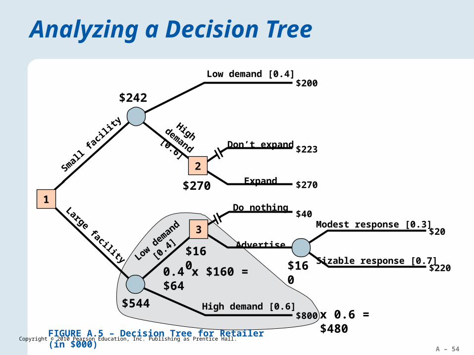
x 0.6 = $480
0.4 x $160 = $64
$544
A – 55
Copyright © 2010 Pearson Education, Inc. Publishing as Prentice Hall.
Analyzing a Decision Tree
$200
$223
$270
$40
$800
$20
$220
Don’t expand
Expand
Low demand [0.4]
High demand
[0.6]
2
FIGURE A.5 – Decision Tree for Retailer (in $000)
Low dem
and
[0.4]
High demand [0.6]
3
Do nothing
Advertise
Modest response [0.3]
Sizable response [0.7]
Smal
l fac
ility
Large facility
1
$160$160
$270
$242
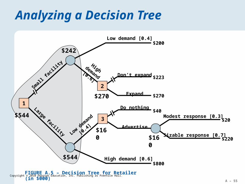
$544
$544
A – 56
Copyright © 2010 Pearson Education, Inc. Publishing as Prentice Hall.
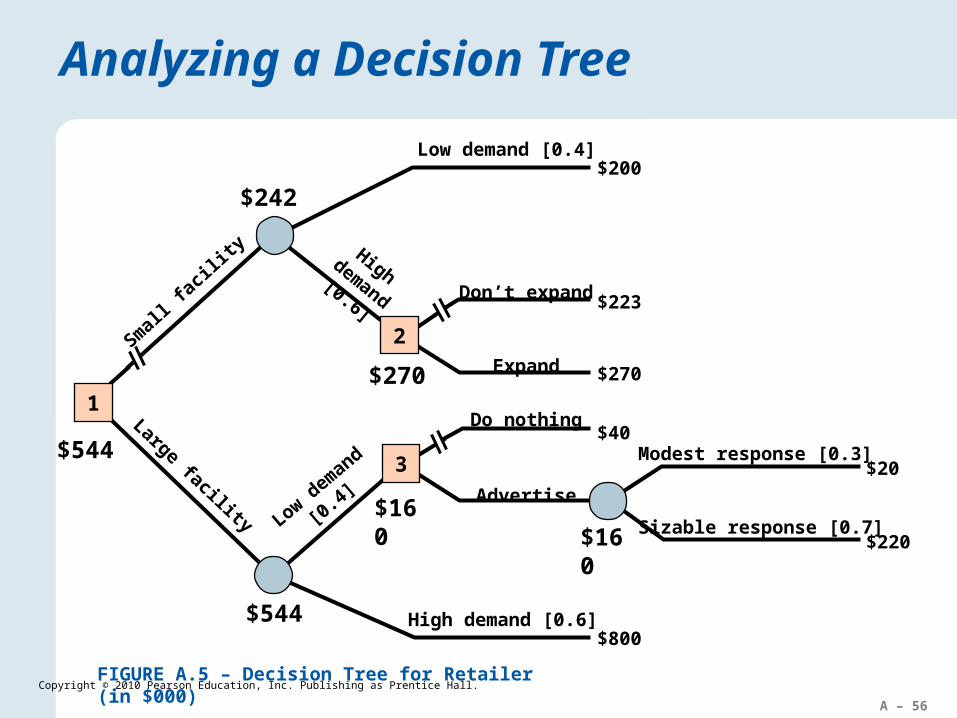
Analyzing a Decision Tree
$200
$223
$270
$40
$800
$20
$220
Don’t expand
Expand
Low demand [0.4]
High demand
[0.6]
2
FIGURE A.5 – Decision Tree for Retailer (in $000)
Low dem
and
[0.4]
High demand [0.6]
3
Do nothing
Advertise
Modest response [0.3]
Sizable response [0.7]
Smal
l fac
ility
Large facility
1
$160$160
$270
$242
$544
$544
A – 57
Copyright © 2010 Pearson Education, Inc. Publishing as Prentice Hall.
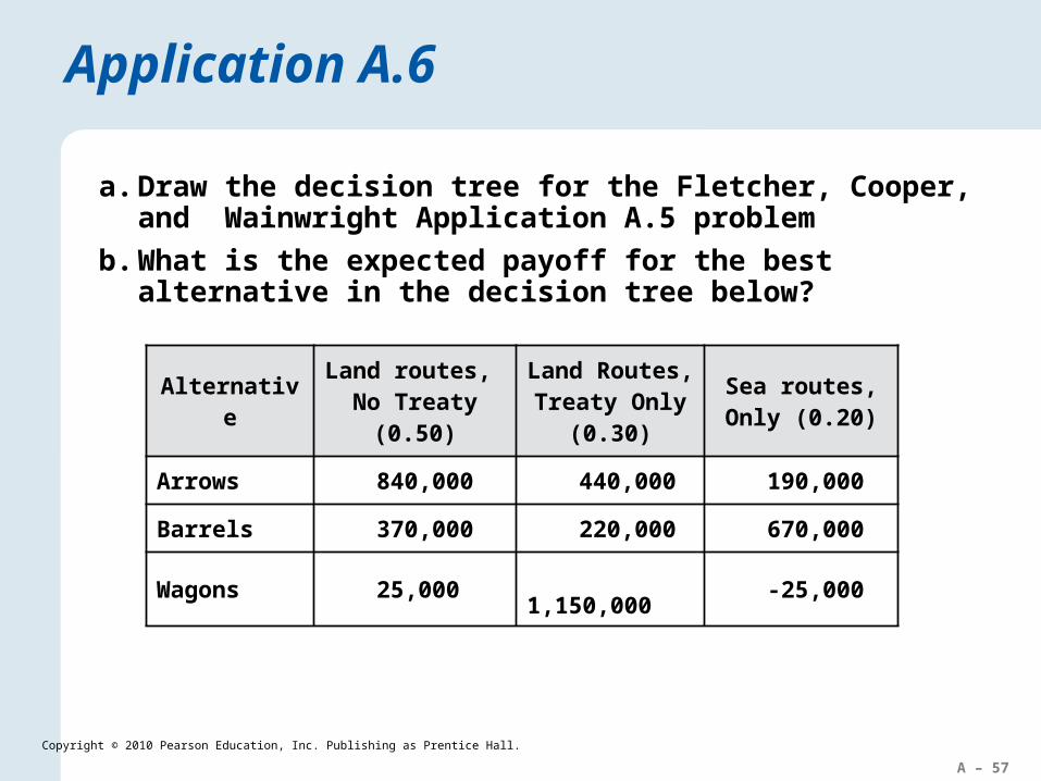
Application A.6
a. Draw the decision tree for the Fletcher, Cooper, and Wainwright Application A.5 problem
b. What is the expected payoff for the best alternative in the decision tree below?
AlternativeLand routes,
No Treaty(0.50)
Land Routes, Treaty Only
(0.30)
Sea routes, Only (0.20)
Arrows 840,000 440,000 190,000
Barrels 370,000 220,000 670,000
Wagons 25,000 1,150,000-
25,000
A – 58
Copyright © 2010 Pearson Education, Inc. Publishing as Prentice Hall.
Application A.6
A – 59
Copyright © 2010 Pearson Education, Inc. Publishing as Prentice Hall.
Solved Problem 1
A small manufacturing business has patented a new device for washing dishes and cleaning dirty kitchen sinks
The owner wants reasonable assurance of success Variable costs are estimated at $7 per unit produced and
sold Fixed costs are about $56,000 per year
a. If the selling price is set at $25, how many units must be produced and sold to break even? Use both algebraic and graphic approaches.
b. Forecasted sales for the first year are 10,000 units if the price is reduced to $15. With this pricing strategy, what would be the product’s total contribution to profits in the first year?
A – 60
Copyright © 2010 Pearson Education, Inc. Publishing as Prentice Hall.
Solved Problem 1
SOLUTION
a. Beginning with the algebraic approach, we get
Q =F
p – c
= 3,111 units
=56,00025 – 7
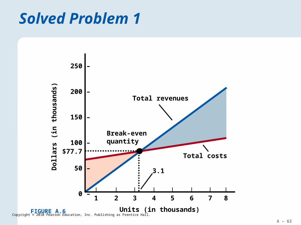
Using the graphic approach, shown in Figure A.6, we first draw two lines:
The two lines intersect at Q = 3,111 units, the break-even quantity
Total revenue =
Total cost =
25Q
56,000 + 7Q
A – 61
Copyright © 2010 Pearson Education, Inc. Publishing as Prentice Hall.
Solved Problem 1
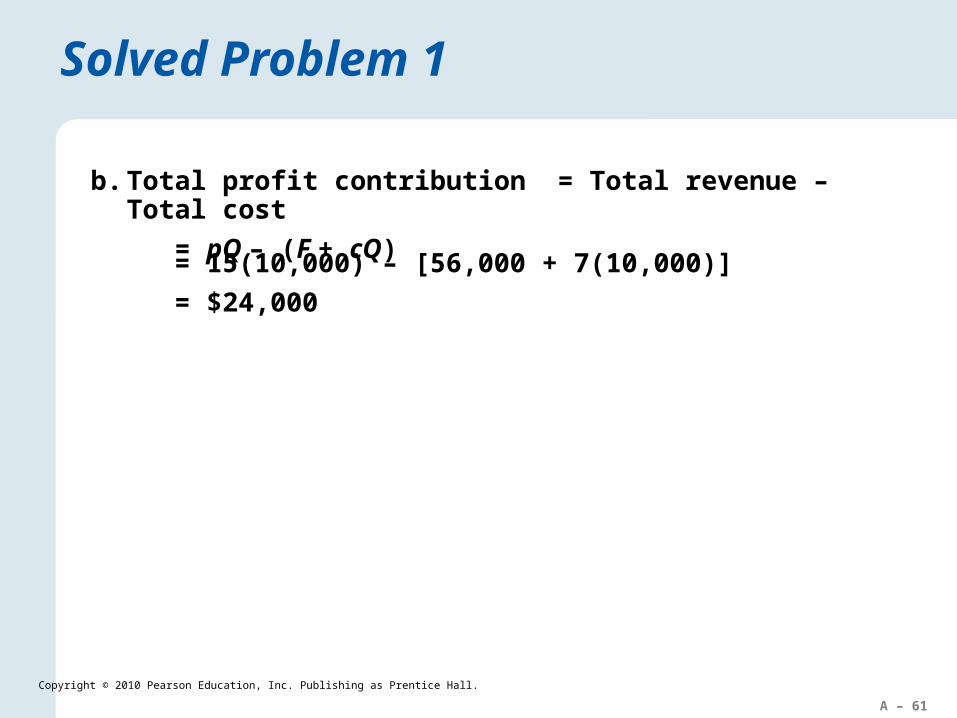
b. Total profit contribution = Total revenue – Total cost
= pQ – (F + cQ)
= 15(10,000) – [56,000 + 7(10,000)]
= $24,000
A – 62
Copyright © 2010 Pearson Education, Inc. Publishing as Prentice Hall.
Total costs
Break-evenquantity
250 –
200 –
150 –
100 –
50 –
0 –
Units (in thousands)
Do
llars
(in
th
ou
san
ds)
| | | | | | | |
1 2 3 4 5 6 7 8
Total revenues
3.1
$77.7
Solved Problem 1
FIGURE A.6
A – 63
Copyright © 2010 Pearson Education, Inc. Publishing as Prentice Hall.
Solved Problem 2
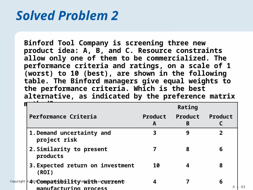
Binford Tool Company is screening three new product idea: A, B, and C. Resource constraints allow only one of them to be commercialized. The performance criteria and ratings, on a scale of 1 (worst) to 10 (best), are shown in the following table. The Binford managers give equal weights to the performance criteria. Which is the best alternative, as indicated by the preference matrix method?
Rating
Performance Criteria Product A Product B Product C
1. Demand uncertainty and project risk3
9 2
2. Similarity to present products7
8 6
3. Expected return on investment (ROI)10
4 8
4. Compatibility with current manufacturing process 4
7 6
5. Competitive Strategy4
6 5
A – 64
Copyright © 2010 Pearson Education, Inc. Publishing as Prentice Hall.
Solved Problem 2
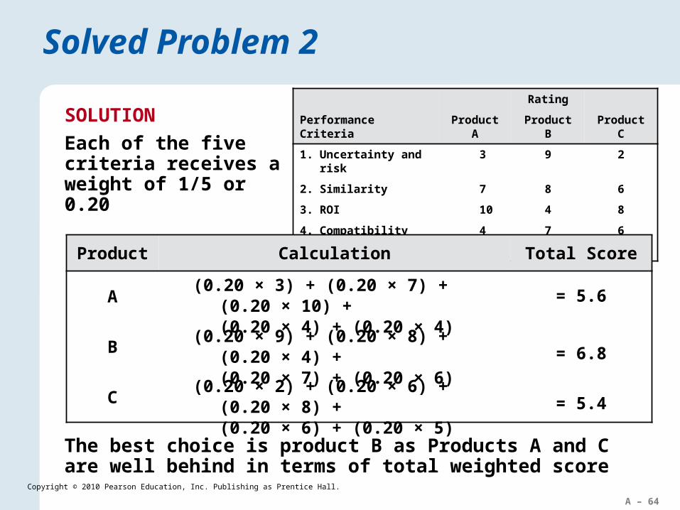
SOLUTION
Each of the five criteria receives a weight of 1/5 or 0.20
Rating
Performance Criteria Product A Product B Product C
1. Uncertainty and risk3
9 2
2. Similarity7
8 6
3. ROI10
4 8
4. Compatibility4
7 6
5. Strategy4
6 5
The best choice is product B as Products A and C are well behind in terms of total weighted score
(0.20 × 3) + (0.20 × 7) + (0.20 × 10) + (0.20 × 4) + (0.20 × 4) = 5.6
(0.20 × 9) + (0.20 × 8) + (0.20 × 4) + (0.20 × 7) + (0.20 × 6) = 6.8
(0.20 × 2) + (0.20 × 6) + (0.20 × 8) + (0.20 × 6) + (0.20 × 5) = 5.4
Product Calculation Total Score
A
B
C
A – 65
Copyright © 2010 Pearson Education, Inc. Publishing as Prentice Hall.
Solved Problem 3
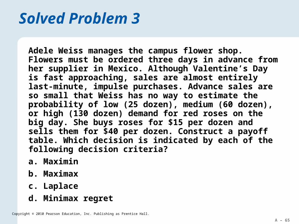
Adele Weiss manages the campus flower shop. Flowers must be ordered three days in advance from her supplier in Mexico. Although Valentine’s Day is fast approaching, sales are almost entirely last-minute, impulse purchases. Advance sales are so small that Weiss has no way to estimate the probability of low (25 dozen), medium (60 dozen), or high (130 dozen) demand for red roses on the big day. She buys roses for $15 per dozen and sells them for $40 per dozen. Construct a payoff table. Which decision is indicated by each of the following decision criteria?
a. Maximin
b. Maximax
c. Laplace
d. Minimax regret
A – 66
Copyright © 2010 Pearson Education, Inc. Publishing as Prentice Hall.
Solved Problem 3
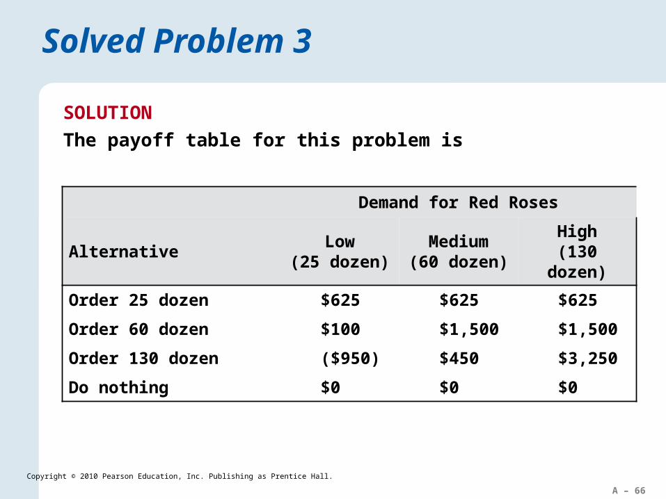
SOLUTION
The payoff table for this problem is
Demand for Red Roses
Alternative Low(25 dozen)
Medium(60 dozen)
High(130 dozen)
Order 25 dozen $625 $625 $625
Order 60 dozen $100 $1,500 $1,500
Order 130 dozen ($950) $450 $3,250
Do nothing $0 $0 $0
A – 67
Copyright © 2010 Pearson Education, Inc. Publishing as Prentice Hall.
Solved Problem 3
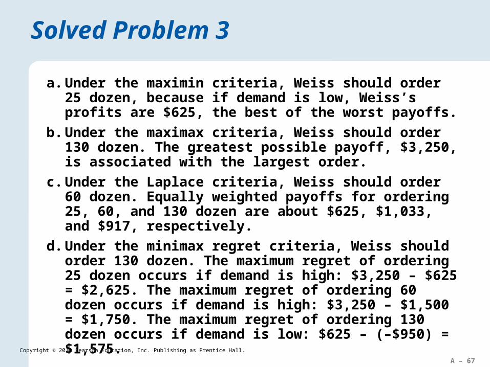
a. Under the maximin criteria, Weiss should order 25 dozen, because if demand is low, Weiss’s profits are $625, the best of the worst payoffs.
b. Under the maximax criteria, Weiss should order 130 dozen. The greatest possible payoff, $3,250, is associated with the largest order.
c. Under the Laplace criteria, Weiss should order 60 dozen. Equally weighted payoffs for ordering 25, 60, and 130 dozen are about $625, $1,033, and $917, respectively.
d. Under the minimax regret criteria, Weiss should order 130 dozen. The maximum regret of ordering 25 dozen occurs if demand is high: $3,250 – $625 = $2,625. The maximum regret of ordering 60 dozen occurs if demand is high: $3,250 – $1,500 = $1,750. The maximum regret of ordering 130 dozen occurs if demand is low: $625 – (–$950) = $1,575.
A – 68
Copyright © 2010 Pearson Education, Inc. Publishing as Prentice Hall.
Solved Problem 4
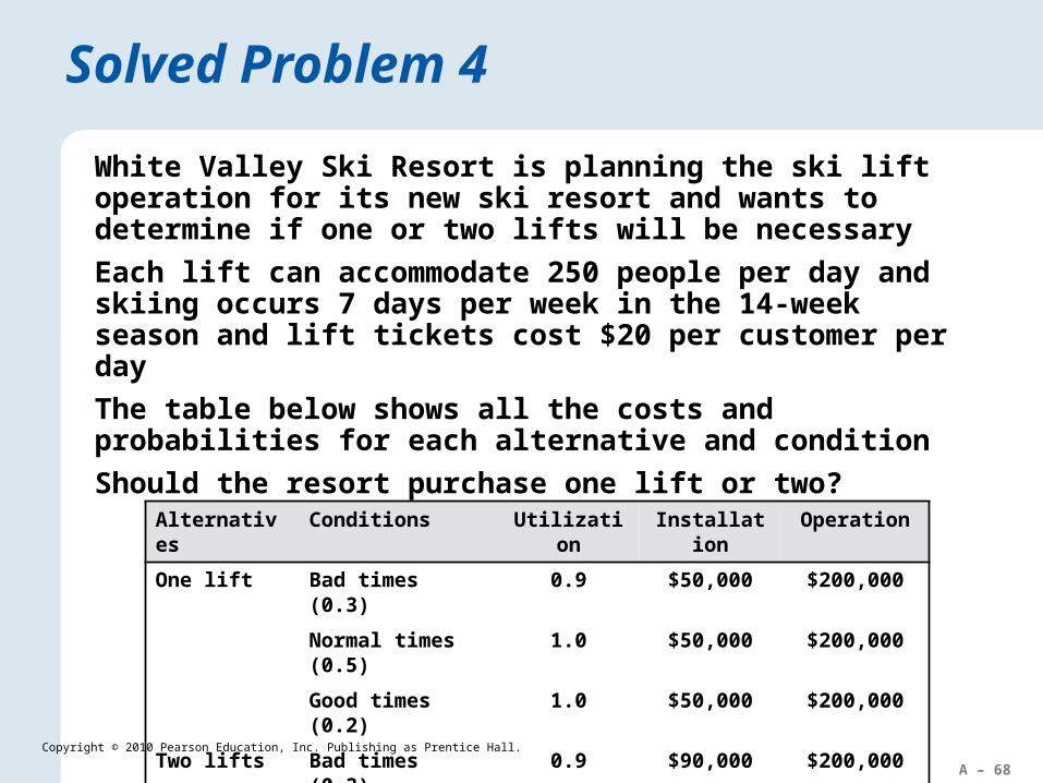
White Valley Ski Resort is planning the ski lift operation for its new ski resort and wants to determine if one or two lifts will be necessary
Each lift can accommodate 250 people per day and skiing occurs 7 days per week in the 14-week season and lift tickets cost $20 per customer per day
The table below shows all the costs and probabilities for each alternative and condition
Should the resort purchase one lift or two?
Alternatives Conditions Utilization Installation Operation
One lift Bad times (0.3) 0.9 $50,000 $200,000
Normal times (0.5) 1.0 $50,000 $200,000
Good times (0.2) 1.0 $50,000 $200,000
Two lifts Bad times (0.3) 0.9 $90,000 $200,000
Normal times (0.5) 1.0 $90,000 $400,000
Good times (0.2) 1.0 $90,000 $400,000
A – 69
Copyright © 2010 Pearson Education, Inc. Publishing as Prentice Hall.
Solved Problem 4
SOLUTION
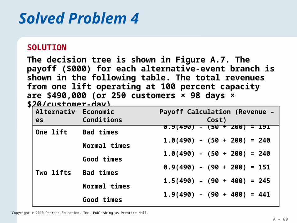
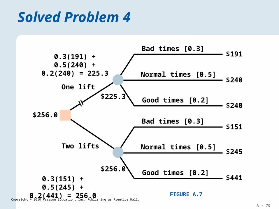
The decision tree is shown in Figure A.7. The payoff ($000) for each alternative-event branch is shown in the following table. The total revenues from one lift operating at 100 percent capacity are $490,000 (or 250 customers × 98 days × $20/customer-day).
0.9(490) – (50 + 200) = 191
1.0(490) – (50 + 200) = 240
1.0(490) – (50 + 200) = 240
0.9(490) – (90 + 200) = 151
1.5(490) – (90 + 400) = 245
1.9(490) – (90 + 400) = 441
Alternatives Economic Conditions Payoff Calculation (Revenue – Cost)
One lift Bad times
Normal times
Good times
Two lifts Bad times
Normal times
Good times
A – 70
Copyright © 2010 Pearson Education, Inc. Publishing as Prentice Hall.
Bad times [0.3]
Normal times [0.5]
Good times [0.2]
$191
$240
$240
Bad times [0.3]
Normal times [0.5]
Good times [0.2]
$151
$245
$441
One lift
Two lifts
$256.0
$225.3
$256.0
Solved Problem 4
0.3(191) + 0.5(240) + 0.2(240) = 225.3
0.3(151) + 0.5(245) + 0.2(441) = 256.0
FIGURE A.7
A – 71
Copyright © 2010 Pearson Education, Inc. Publishing as Prentice Hall.