Embed Size (px)
Citation preview

H – 1Copyright © 2010 Pearson Education, Inc. Publishing as Prentice Hall.
Measuring Output RatesMeasuring Output RatesH
For For Operations Management, 9eOperations Management, 9e by by Krajewski/Ritzman/Malhotra Krajewski/Ritzman/Malhotra © 2010 Pearson Education© 2010 Pearson Education
PowerPoint Slides PowerPoint Slides by Jeff Heylby Jeff Heyl

H – 2Copyright © 2010 Pearson Education, Inc. Publishing as Prentice Hall.
Work Standards Work Standards
A work standard is the time required for a trained worker to perform a task following a prescribed method with normal effort and skill
Used in the following ways: Establishing prices and costs Motivating workers Comparing alternative process designs Scheduling Capacity planning Performance appraisal
H – 3Copyright © 2010 Pearson Education, Inc. Publishing as Prentice Hall.
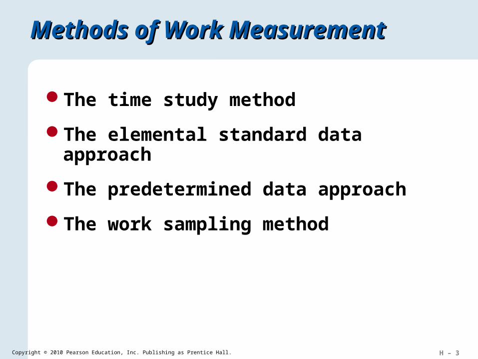
Methods of Work Measurement Methods of Work Measurement
The time study method
The elemental standard data approach
The predetermined data approach
The work sampling method
H – 4Copyright © 2010 Pearson Education, Inc. Publishing as Prentice Hall.
The Time Study MethodThe Time Study Method
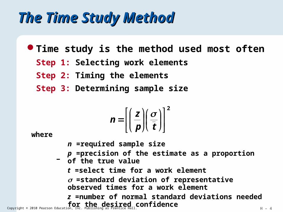
Time study is the method used most often Step 1: Selecting work elements
Step 2: Timing the elements
Step 3: Determining sample size2
tpz
n
wheren =required sample sizep =precision of the estimate as a proportion of the true valuet =select time for a work element =standard deviation of representative observed times for a work elementz =number of normal standard deviations needed for the desired confidence
H – 5Copyright © 2010 Pearson Education, Inc. Publishing as Prentice Hall.
The Time Study MethodThe Time Study Method
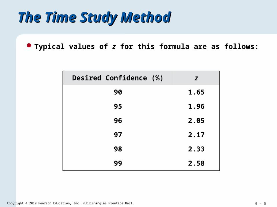
Typical values of z for this formula are as follows:
Desired Confidence (%) z
90 1.65
95 1.96
96 2.05
97 2.17
98 2.33
99 2.58
H – 6Copyright © 2010 Pearson Education, Inc. Publishing as Prentice Hall.
Estimating the Sample Size in a Estimating the Sample Size in a Time StudyTime Study
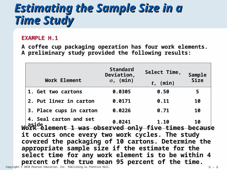
EXAMPLE H.1
A coffee cup packaging operation has four work elements. A preliminary study provided the following results:
Work Element
Standard Deviation, , (min)
Select Time, t, (min)
Sample Size
1. Get two cartons 0.0305 0.50 5
2. Put liner in carton 0.0171 0.11 10
3. Place cups in carton 0.0226 0.71 10
4. Seal carton and set aside 0.0241 1.10 10
Work element 1 was observed only five times because it occurs once every two work cycles. The study covered the packaging of 10 cartons. Determine the appropriate sample size if the estimate for the select time for any work element is to be within 4 percent of the true mean 95 percent of the time.
H – 7Copyright © 2010 Pearson Education, Inc. Publishing as Prentice Hall.
Estimating the Sample Size in a Estimating the Sample Size in a Time StudyTime Study
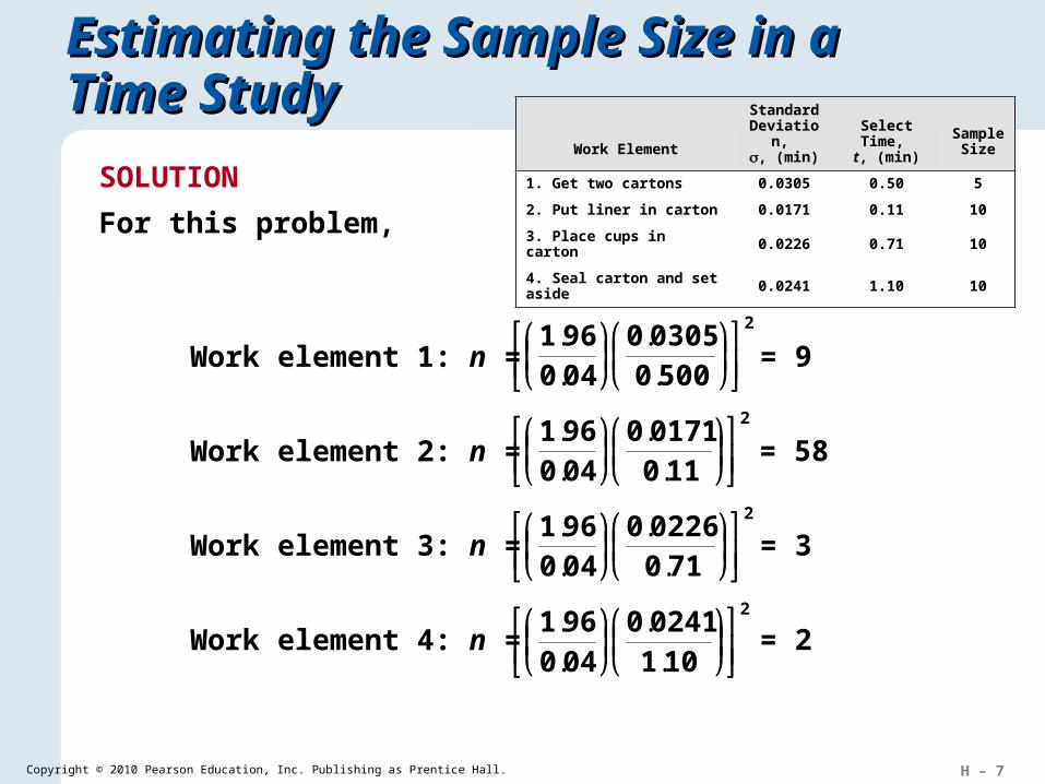
SOLUTION
For this problem,
Work Element
Standard Deviation, , (min)
Select Time, t, (min)
Sample Size
1. Get two cartons 0.0305 0.50 5
2. Put liner in carton 0.0171 0.11 10
3. Place cups in carton 0.0226 0.71 10
4. Seal carton and set aside 0.0241 1.10 10
Work element 1: n =
Work element 2: n =
Work element 3: n =
Work element 4: n =
2
500003050
040961
..
.
.= 9
2
11001710
040961
..
.
.= 58
2
71002260
040961
..
.
.= 3
2
10102410
040961
..
.
.= 2
H – 8Copyright © 2010 Pearson Education, Inc. Publishing as Prentice Hall.
The Time Study MethodThe Time Study Method
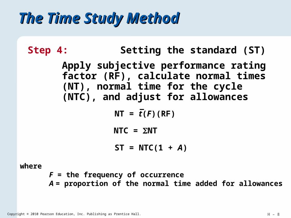
Step 4: Setting the standard (ST)
Apply subjective performance rating factor (RF), calculate normal times (NT), normal time for the cycle (NTC), and adjust for allowances
NTC = NT
ST = NTC(1 + A)
where F = the frequency of occurrenceA = proportion of the normal time added for allowances
NT = t(F)(RF)
H – 9Copyright © 2010 Pearson Education, Inc. Publishing as Prentice Hall.
Determining the Normal TimeDetermining the Normal Time
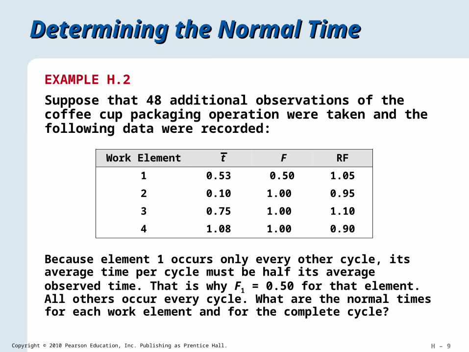
EXAMPLE H.2
Suppose that 48 additional observations of the coffee cup packaging operation were taken and the following data were recorded:
Work Element t F RF
1 0.53 0.50 1.05
2 0.10 1.00 0.95
3 0.75 1.00 1.10
4 1.08 1.00 0.90
Because element 1 occurs only every other cycle, its average time per cycle must be half its average observed time. That is why F1 = 0.50 for that element. All others occur every cycle. What are the normal times for each work element and for the complete cycle?
H – 10Copyright © 2010 Pearson Education, Inc. Publishing as Prentice Hall.
Determining the Normal TimeDetermining the Normal Time
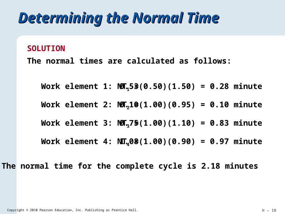
SOLUTION
The normal times are calculated as follows:
Work element 1: NT1 =
Work element 2: NT2 =
Work element 3: NT3 =
Work element 4: NT4 =
0.53(0.50)(1.50) = 0.28 minute
0.10(1.00)(0.95) = 0.10 minute
0.75(1.00)(1.10) = 0.83 minute
1.08(1.00)(0.90) = 0.97 minute
The normal time for the complete cycle is 2.18 minutes
H – 11Copyright © 2010 Pearson Education, Inc. Publishing as Prentice Hall.
Determining the Standard Time
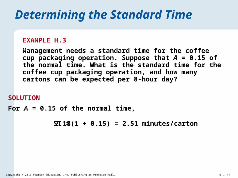
EXAMPLE H.3
Management needs a standard time for the coffee cup packaging operation. Suppose that A = 0.15 of the normal time. What is the standard time for the coffee cup packaging operation, and how many cartons can be expected per 8-hour day?
SOLUTION
For A = 0.15 of the normal time,
ST = 2.18(1 + 0.15) = 2.51 minutes/carton

H – 12Copyright © 2010 Pearson Education, Inc. Publishing as Prentice Hall.
Application H.1Application H.1
Lucy and Ethel have repetitive jobs at the candy factory. Management desires to establish a time standard for this work for which they can be 95% confident to be within ± 6% of the true mean. There are three work elements involved:
SOLUTION
Step 1: Selecting work elements
#1: Pick up wrapper paper and wrap one piece of candy
#2: Put candy in a box, one at a time
#3: When the box is full (4 pieces), close it and place on conveyor
H – 13Copyright © 2010 Pearson Education, Inc. Publishing as Prentice Hall.
Application H.1Application H.1
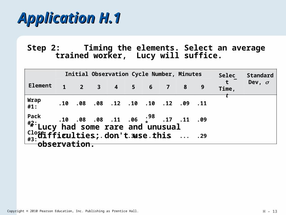
Step 2: Timing the elements. Select an average trained worker, Lucy will suffice.
Element
Initial Observation Cycle Number, Minutes
1 2 3 4 5 6 7 8 9
Wrap #1: .10 .08 .08 .12 .10 .10 .12 .09 .11
Pack #2: .10 .08 .08 .11 .06 .98* .17 .11 .09
Close #3: .27 ... ... ... .34 ... ... ... .29
SelectTime, t
Standard Dev,
* Lucy had some rare and unusual difficulties; don't use this observation.
H – 14Copyright © 2010 Pearson Education, Inc. Publishing as Prentice Hall.
Application H.1Application H.1
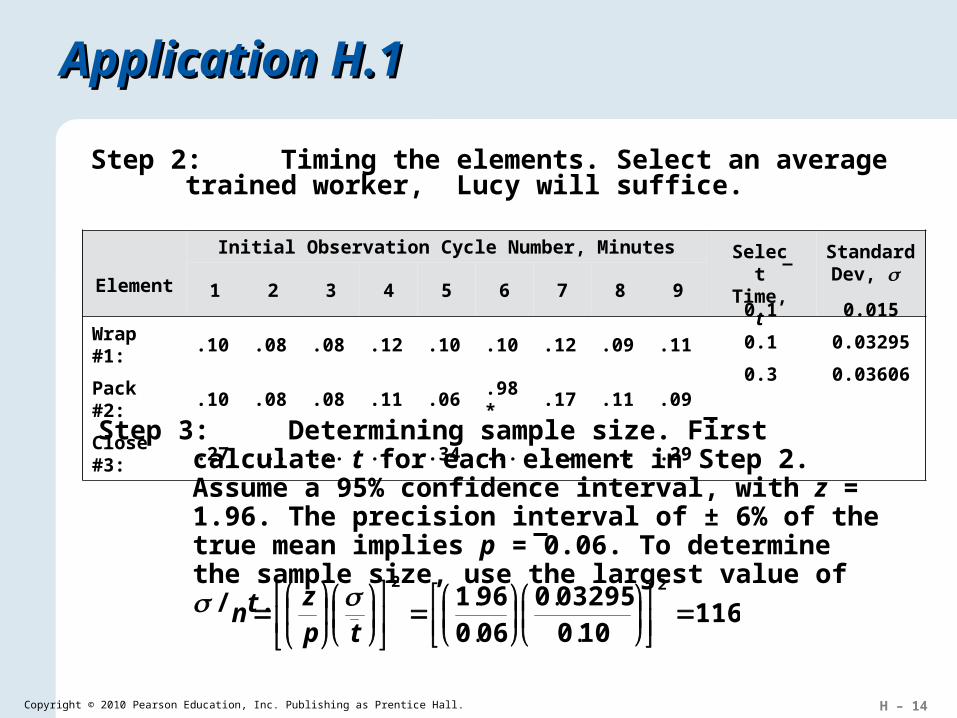
Step 2: Timing the elements. Select an average trained worker, Lucy will suffice.
Element
Initial Observation Cycle Number, Minutes
1 2 3 4 5 6 7 8 9
Wrap #1: .10 .08 .08 .12 .10 .10 .12 .09 .11
Pack #2: .10 .08 .08 .11 .06 .98* .17 .11 .09
Close #3: .27 ... ... ... .34 ... ... ... .29
SelectTime, t
Standard Dev,
0.1 0.015
0.1 0.03295
0.3 0.03606
Step 3: Determining sample size. First calculate t for each element in Step 2. Assume a 95% confidence interval, with z = 1.96. The precision interval of ± 6% of the true mean implies p = 0.06. To determine the sample size, use the largest value of / t .
116100
032950060961
22
..
.
.tp
zn
H – 15Copyright © 2010 Pearson Education, Inc. Publishing as Prentice Hall.
Element Select Time, t Frequency Rating Factor Normal Time
Wrap #1: 1.00 1.2
Pack #2: 1.00 0.9
Close #3: 0.25 0.8
Application H.1Application H.1
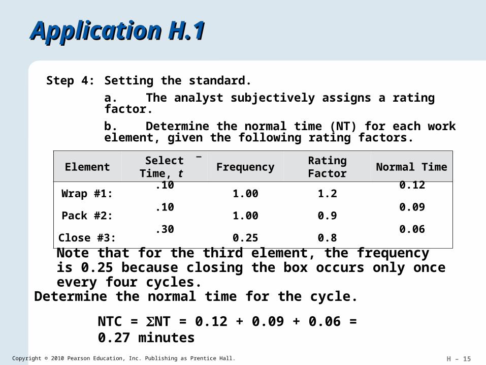
Step 4: Setting the standard.
a. The analyst subjectively assigns a rating factor.
b. Determine the normal time (NT) for each work element, given the following rating factors.
.10
.10
.30
0.12
0.09
0.06
Note that for the third element, the frequency is 0.25 because closing the box occurs only once every four cycles.
c. Determine the normal time for the cycle.
NTC = NT = 0.12 + 0.09 + 0.06 = 0.27 minutes
H – 16Copyright © 2010 Pearson Education, Inc. Publishing as Prentice Hall.
Element Select Time, t Frequency Rating Factor Normal Time
Wrap #1: 1.00 1.2
Pack #2: 1.00 0.9
Close #3: 0.25 0.8
Application H.1Application H.1
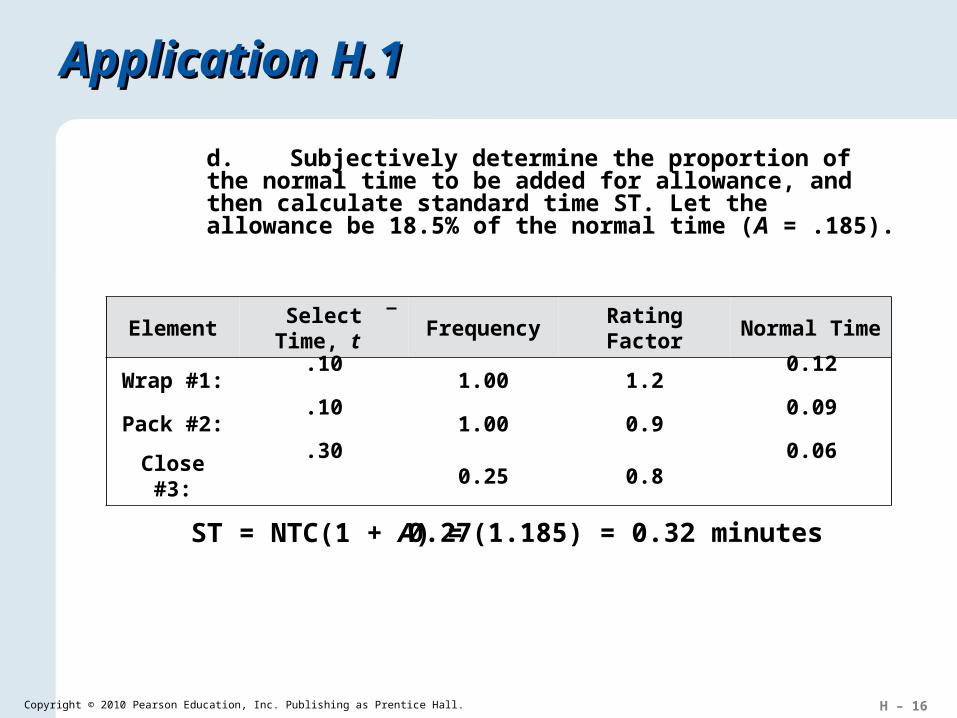
d. Subjectively determine the proportion of the normal time to be added for allowance, and then calculate standard time ST. Let the allowance be 18.5% of the normal time (A = .185).
.10
.10
.30
0.12
0.09
0.06
ST = NTC(1 + A) = 0.27(1.185) = 0.32 minutes
H – 17Copyright © 2010 Pearson Education, Inc. Publishing as Prentice Hall.
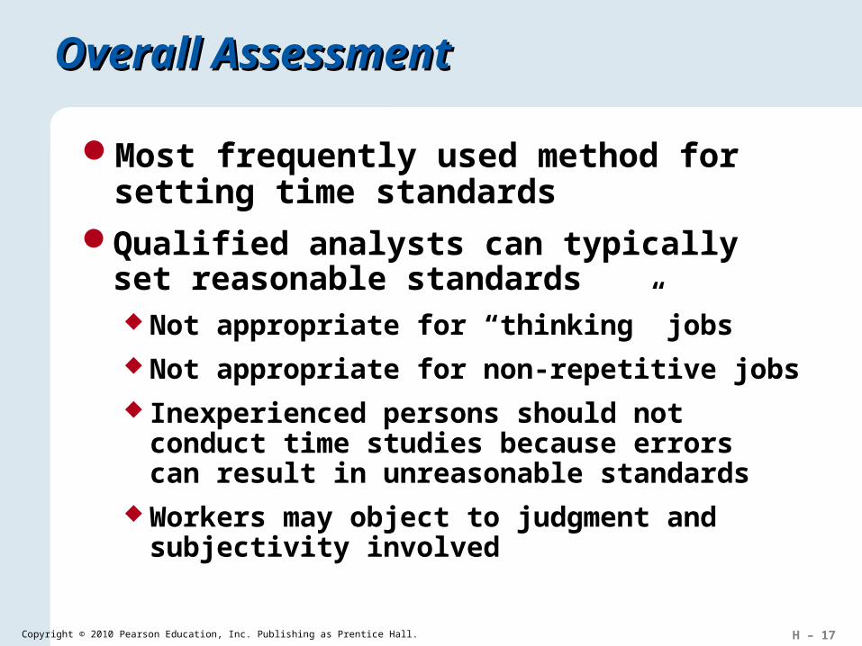
Overall AssessmentOverall Assessment
Most frequently used method for setting time standards
Qualified analysts can typically set reasonable standards Not appropriate for “thinking” jobs Not appropriate for non-repetitive jobs Inexperienced persons should not conduct time
studies because errors can result in unreasonable standards
Workers may object to judgment and subjectivity involved
H – 18Copyright © 2010 Pearson Education, Inc. Publishing as Prentice Hall.
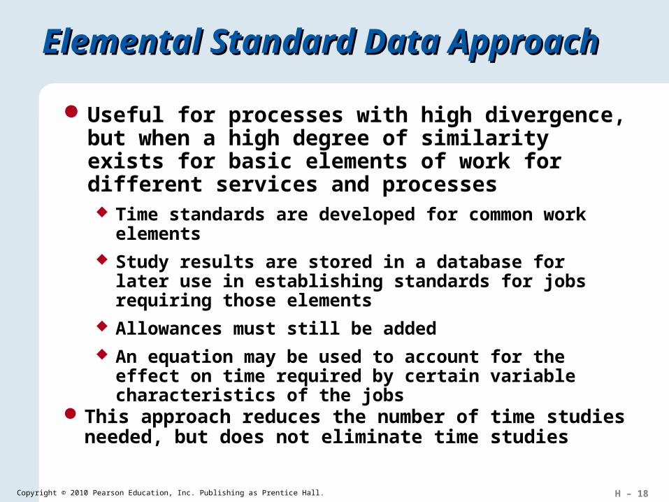
Elemental Standard Data ApproachElemental Standard Data Approach
Useful for processes with high divergence, but when a high degree of similarity exists for basic elements of work for different services and processes Time standards are developed for common work
elements Study results are stored in a database for later use in
establishing standards for jobs requiring those elements Allowances must still be added An equation may be used to account for the effect on
time required by certain variable characteristics of the jobs
This approach reduces the number of time studies needed, but does not eliminate time studies
H – 19Copyright © 2010 Pearson Education, Inc. Publishing as Prentice Hall.
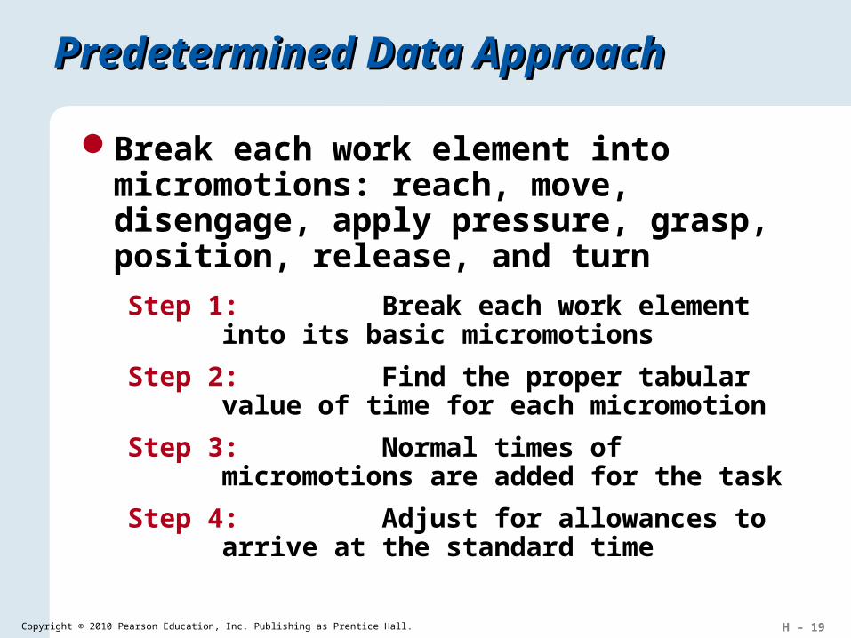
Predetermined Data ApproachPredetermined Data Approach
Break each work element into micromotions: reach, move, disengage, apply pressure, grasp, position, release, and turn
Step 1: Break each work element into its basic micromotions
Step 2: Find the proper tabular value of time for each micromotion
Step 3: Normal times of micromotions are added for the task
Step 4: Adjust for allowances to arrive at the standard time
H – 20Copyright © 2010 Pearson Education, Inc. Publishing as Prentice Hall.
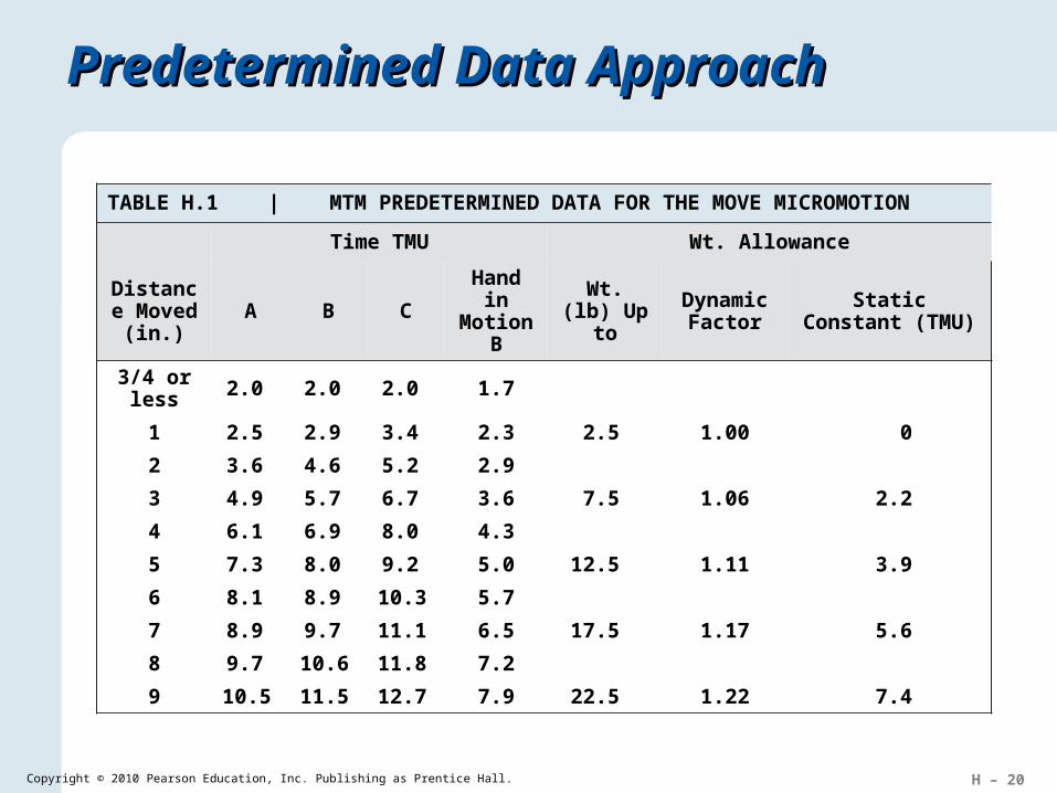
TABLE H.1 | MTM PREDETERMINED DATA FOR THE MOVE MICROMOTION
Time TMU Wt. Allowance
Distance Moved
(in.)A B C
Hand in Motion
B
Wt. (lb) Up to
Dynamic Factor
Static Constant (TMU)
3/4 or less 2.0 2.0 2.0 1.7
1 2.5 2.9 3.4 2.3 2.5 1.00 0
2 3.6 4.6 5.2 2.9
3 4.9 5.7 6.7 3.6 7.5 1.06 2.2
4 6.1 6.9 8.0 4.3
5 7.3 8.0 9.2 5.0 12.5 1.11 3.9
6 8.1 8.9 10.3 5.7
7 8.9 9.7 11.1 6.5 17.5 1.17 5.6
8 9.7 10.6 11.8 7.2
9 10.5 11.5 12.7 7.9 22.5 1.22 7.4
Predetermined Data ApproachPredetermined Data Approach
H – 21Copyright © 2010 Pearson Education, Inc. Publishing as Prentice Hall.
Predetermined Data ApproachPredetermined Data Approach
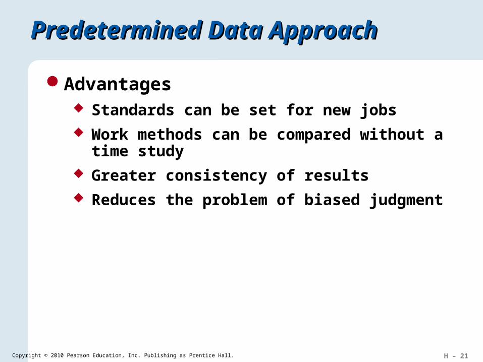
Advantages Standards can be set for new jobs Work methods can be compared without a
time study Greater consistency of results Reduces the problem of biased judgment
H – 22Copyright © 2010 Pearson Education, Inc. Publishing as Prentice Hall.
Predetermined Data ApproachPredetermined Data Approach
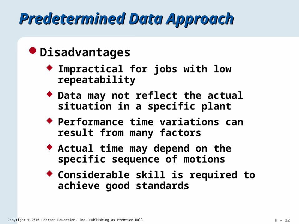
Disadvantages Impractical for jobs with low repeatability Data may not reflect the actual situation in a
specific plant Performance time variations can result from
many factors Actual time may depend on the specific
sequence of motions Considerable skill is required to achieve good
standards
H – 23Copyright © 2010 Pearson Education, Inc. Publishing as Prentice Hall.
Work Sampling Method Work Sampling Method
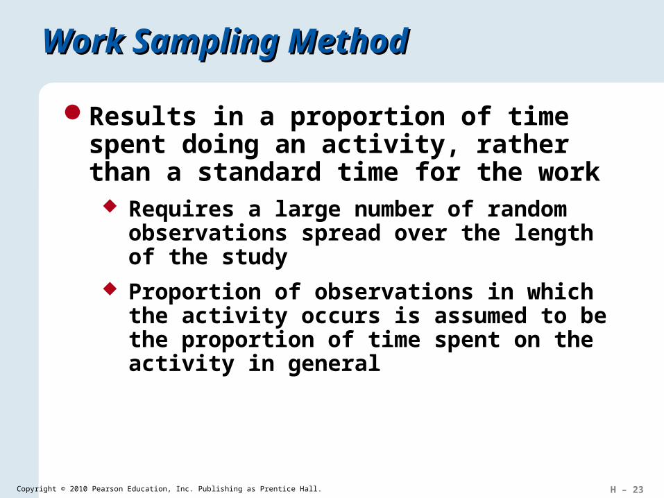
Results in a proportion of time spent doing an activity, rather than a standard time for the work
Requires a large number of random observations spread over the length of the study
Proportion of observations in which the activity occurs is assumed to be the proportion of time spent on the activity in general
H – 24Copyright © 2010 Pearson Education, Inc. Publishing as Prentice Hall.
Work Sampling Method Work Sampling Method
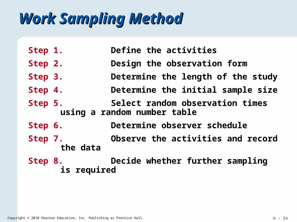
Step 1. Define the activities
Step 2. Design the observation form
Step 3. Determine the length of the study
Step 4. Determine the initial sample size
Step 5. Select random observation times using a random number table
Step 6. Determine observer schedule
Step 7. Observe the activities and record the data
Step 8. Decide whether further sampling is required
H – 25Copyright © 2010 Pearson Education, Inc. Publishing as Prentice Hall.
Work Sampling Method Work Sampling Method
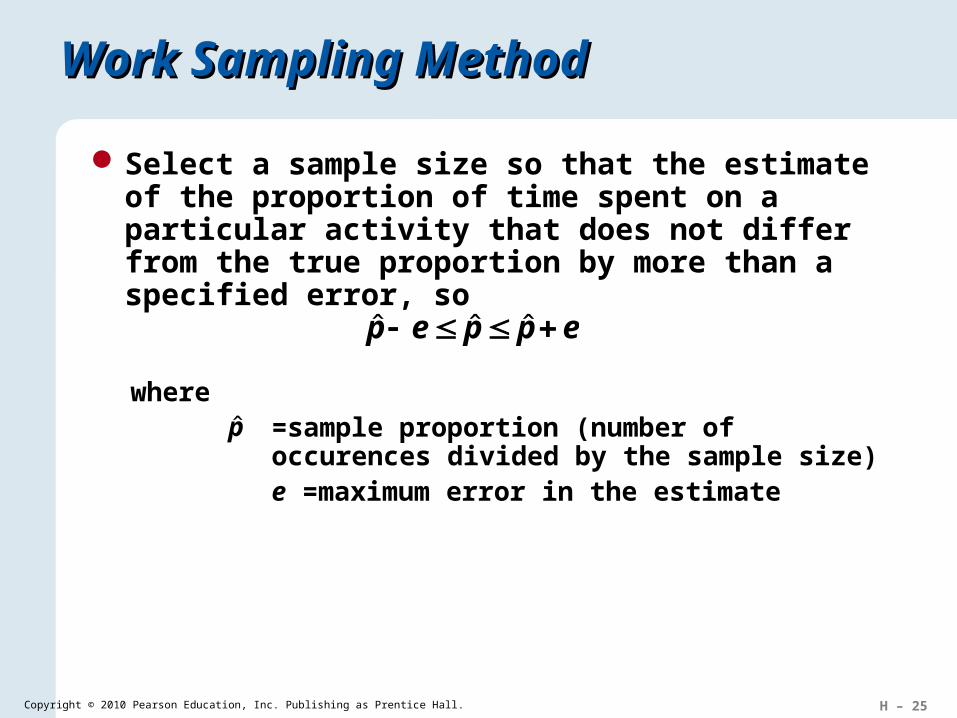
Select a sample size so that the estimate of the proportion of time spent on a particular activity that does not differ from the true proportion by more than a specified error, so
eppep ˆˆˆ
where=sample proportion (number of occurences divided by the sample size)e =maximum error in the estimate
p̂
H – 26Copyright © 2010 Pearson Education, Inc. Publishing as Prentice Hall.
Work Sampling Method Work Sampling Method
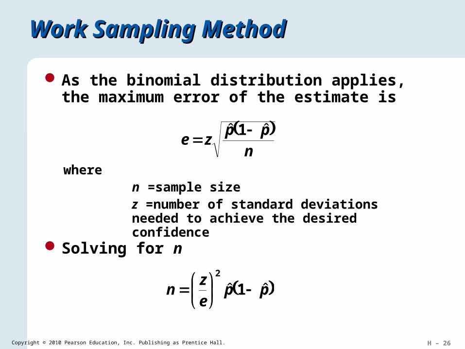
As the binomial distribution applies, the maximum error of the estimate is
n
ppze
ˆˆ
1
wheren =sample sizez =number of standard deviations needed to achieve the desired confidence
Solving for n
ppez
n ˆˆ
1
2
H – 27Copyright © 2010 Pearson Education, Inc. Publishing as Prentice Hall.
Work Sampling Method Work Sampling Method
n
ppze
ˆˆ
1
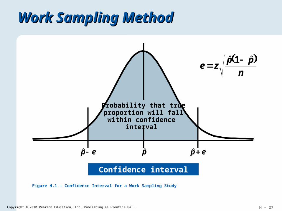
Confidence interval
Probability that trueproportion will fall
within confidence interval
ep ˆ p̂ ep ˆ
Figure H.1 – Confidence Interval for a Work Sampling Study

H – 28Copyright © 2010 Pearson Education, Inc. Publishing as Prentice Hall.
Using Work Sampling DataUsing Work Sampling Data
EXAMPLE H.4
The hospital administrator at a private hospital is considering a proposal for installing an automated medical records storage and retrieval system. To determine the advisability of purchasing such a system, the administrator needs to know the proportion of time that registered nurses (RNs) and licensed vocational nurses (LVNs) spend accessing records. Currently, these nurses must either retrieve the records manually or have them copied and sent to their wards. A typical ward, staffed by eight RNs and four LVNs, is selected for the study.
H – 29Copyright © 2010 Pearson Education, Inc. Publishing as Prentice Hall.
Using Work Sampling DataUsing Work Sampling Data
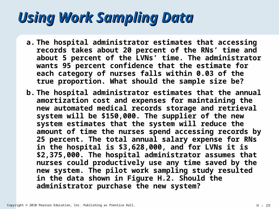
a. The hospital administrator estimates that accessing records takes about 20 percent of the RNs’ time and about 5 percent of the LVNs’ time. The administrator wants 95 percent confidence that the estimate for each category of nurses falls within 0.03 of the true proportion. What should the sample size be?
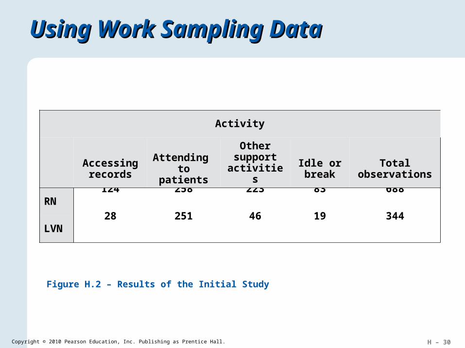
b. The hospital administrator estimates that the annual amortization cost and expenses for maintaining the new automated medical records storage and retrieval system will be $150,000. The supplier of the new system estimates that the system will reduce the amount of time the nurses spend accessing records by 25 percent. The total annual salary expense for RNs in the hospital is $3,628,000, and for LVNs it is $2,375,000. The hospital administrator assumes that nurses could productively use any time saved by the new system. The pilot work sampling study resulted in the data shown in Figure H.2. Should the administrator purchase the new system?
H – 30Copyright © 2010 Pearson Education, Inc. Publishing as Prentice Hall.
124 258 223 83 688
28 251 46 19 344
Using Work Sampling DataUsing Work Sampling Data
Activity
Accessing records
Attending to patients
Other support
activitiesIdle or break
Total observations
RN
LVN
Figure H.2 – Results of the Initial Study
H – 31Copyright © 2010 Pearson Education, Inc. Publishing as Prentice Hall.
Using Work Sampling DataUsing Work Sampling Data
SOLUTION
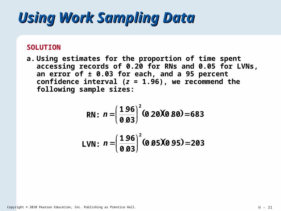
a. Using estimates for the proportion of time spent accessing records of 0.20 for RNs and 0.05 for LVNs, an error of ± 0.03 for each, and a 95 percent confidence interval (z = 1.96), we recommend the following sample sizes:
683800200030961 2
..
.
.n
203950050030961 2
..
.
.n
RN:
LVN:
H – 32Copyright © 2010 Pearson Education, Inc. Publishing as Prentice Hall.
Using Work Sampling DataUsing Work Sampling Data
Eight RNs and four LVNs can be observed on each trip. Therefore, 683/8 = 86 (rounded up) trips are needed for the observations of RNs, and only 203/4 = 51 (rounded up) trips are needed for the LVNs. Thus, 86 trips through the ward will be sufficient for observing both nurse groups. This number of trips will generate 688 observations of RNs and 344 observations of LVNs. It will provide many more observations than are needed for the LVNs, but the added observations may as well be recorded as the observer will be going through the ward anyway.
H – 33Copyright © 2010 Pearson Education, Inc. Publishing as Prentice Hall.
Using Work Sampling DataUsing Work Sampling Data
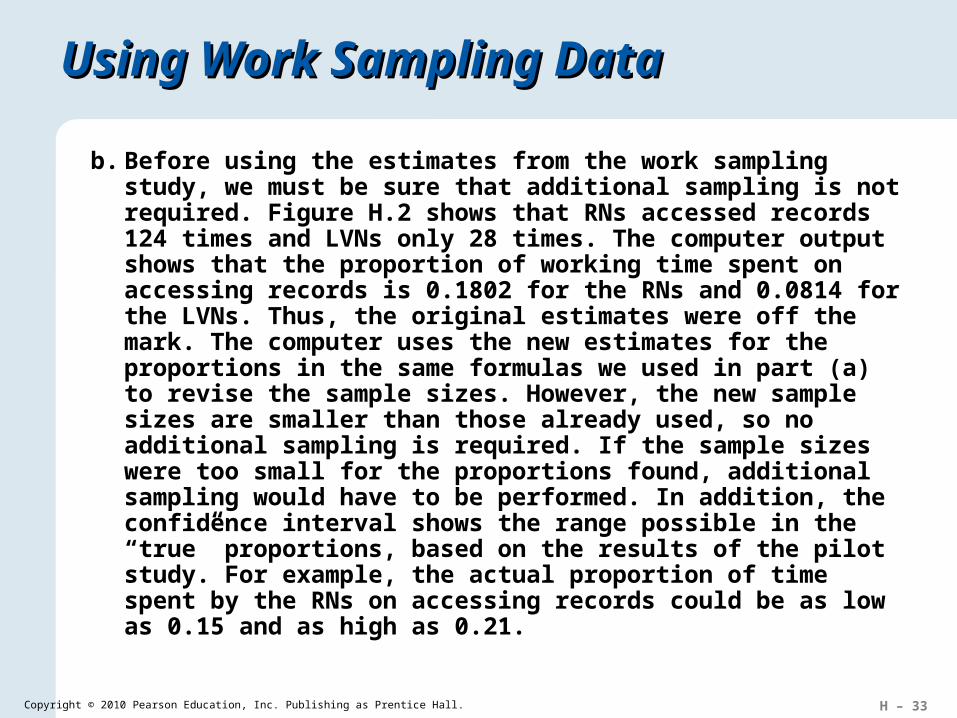
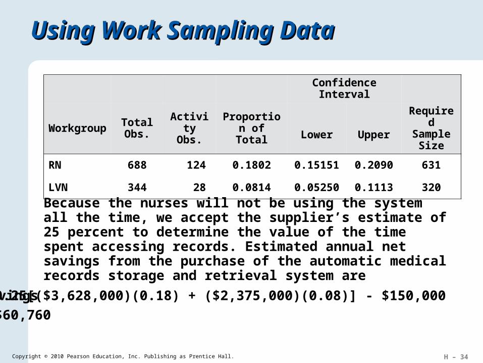
b. Before using the estimates from the work sampling study, we must be sure that additional sampling is not required. Figure H.2 shows that RNs accessed records 124 times and LVNs only 28 times. The computer output shows that the proportion of working time spent on accessing records is 0.1802 for the RNs and 0.0814 for the LVNs. Thus, the original estimates were off the mark. The computer uses the new estimates for the proportions in the same formulas we used in part (a) to revise the sample sizes. However, the new sample sizes are smaller than those already used, so no additional sampling is required. If the sample sizes were too small for the proportions found, additional sampling would have to be performed. In addition, the confidence interval shows the range possible in the “true” proportions, based on the results of the pilot study. For example, the actual proportion of time spent by the RNs on accessing records could be as low as 0.15 and as high as 0.21.
H – 34Copyright © 2010 Pearson Education, Inc. Publishing as Prentice Hall.
Using Work Sampling DataUsing Work Sampling Data
Confidence Interval
Workgroup Total Obs.
Activity Obs.
Proportion of Total Lower Upper
Required Sample
Size
RN 688 124 0.1802 0.15151 0.2090 631
LVN 344 28 0.0814 0.05250 0.1113 320
Because the nurses will not be using the system all the time, we accept the supplier’s estimate of 25 percent to determine the value of the time spent accessing records. Estimated annual net savings from the purchase of the automatic medical records storage and retrieval system are
Net savings = 0.25[($3,628,000)(0.18) + ($2,375,000)(0.08)] - $150,000
= $60,760
H – 35Copyright © 2010 Pearson Education, Inc. Publishing as Prentice Hall.
Application H.2Application H.2
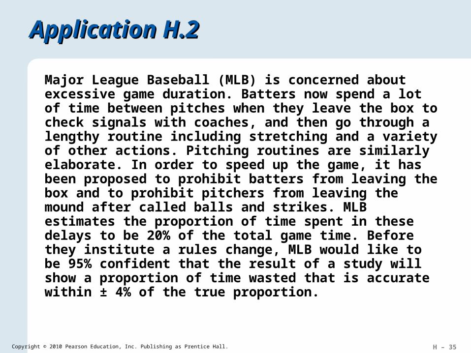
Major League Baseball (MLB) is concerned about excessive game duration. Batters now spend a lot of time between pitches when they leave the box to check signals with coaches, and then go through a lengthy routine including stretching and a variety of other actions. Pitching routines are similarly elaborate. In order to speed up the game, it has been proposed to prohibit batters from leaving the box and to prohibit pitchers from leaving the mound after called balls and strikes. MLB estimates the proportion of time spent in these delays to be 20% of the total game time. Before they institute a rules change, MLB would like to be 95% confident that the result of a study will show a proportion of time wasted that is accurate within ± 4% of the true proportion.
H – 36Copyright © 2010 Pearson Education, Inc. Publishing as Prentice Hall.
Application H.2Application H.2
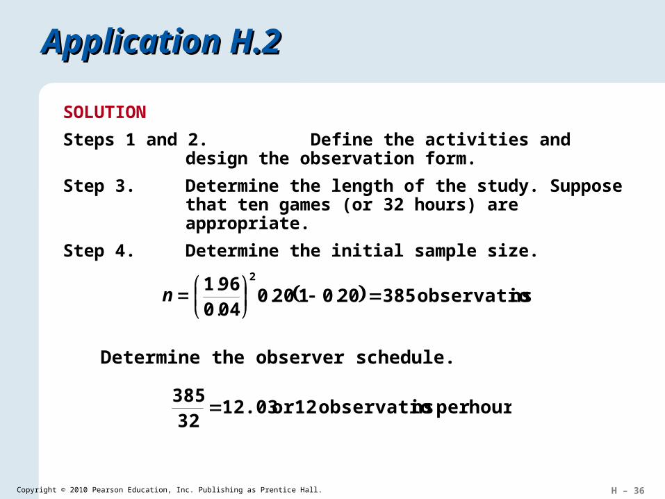
SOLUTION
Steps 1 and 2. Define the activities and design the observation form.
Step 3. Determine the length of the study. Suppose that ten games (or 32 hours) are appropriate.
Step 4. Determine the initial sample size.
nsobservatio 3852001200040961 2
..
.
.n
Steps 5 and 6. Determine the observer schedule.
hour per nsobservatio 12 or 12.0332
385
H – 37Copyright © 2010 Pearson Education, Inc. Publishing as Prentice Hall.
Application H.2Application H.2
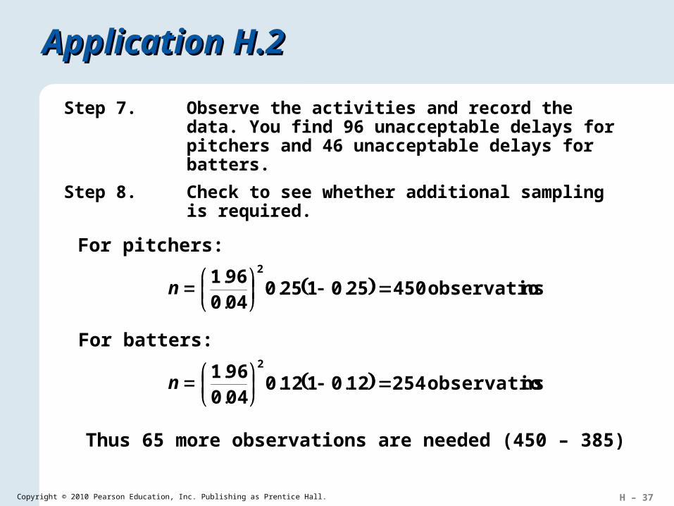
Step 7. Observe the activities and record the data. You find 96 unacceptable delays for pitchers and 46 unacceptable delays for batters.
Step 8. Check to see whether additional sampling is required.
nsobservatio 4502501250040961 2
..
.
.
nsobservatio 2541201120040961 2
..
.
.
For pitchers:
For batters:
n
n
Thus 65 more observations are needed (450 – 385)
H – 38Copyright © 2010 Pearson Education, Inc. Publishing as Prentice Hall.
Overall AssessmentOverall Assessment
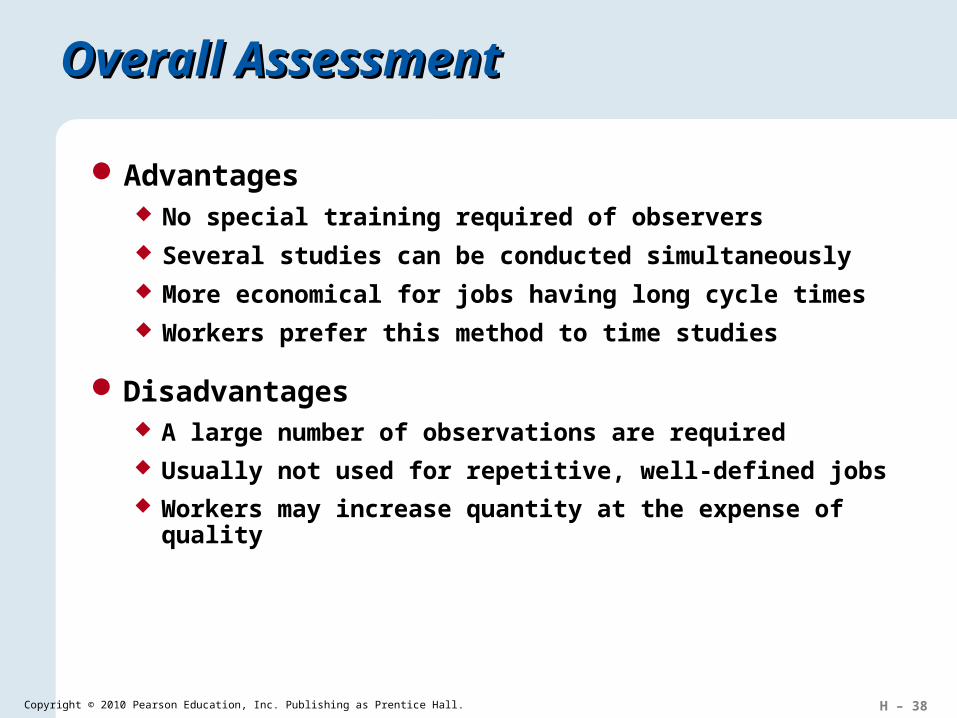
Advantages No special training required of observers Several studies can be conducted simultaneously More economical for jobs having long cycle times Workers prefer this method to time studies
Disadvantages A large number of observations are required Usually not used for repetitive, well-defined jobs Workers may increase quantity at the expense of quality
H – 39Copyright © 2010 Pearson Education, Inc. Publishing as Prentice Hall.
Managerial Considerations Managerial Considerations
Managers should carefully evaluate work measurement techniques to ensure that they are used in ways that are consistent with the firm’s competitive priorities
Technological changes Increased automation There is less need to observe and rate worker
performance, because work is machine paced Work sampling may be electronically
monitored
H – 40Copyright © 2010 Pearson Education, Inc. Publishing as Prentice Hall.
Solved Problem 1Solved Problem 1
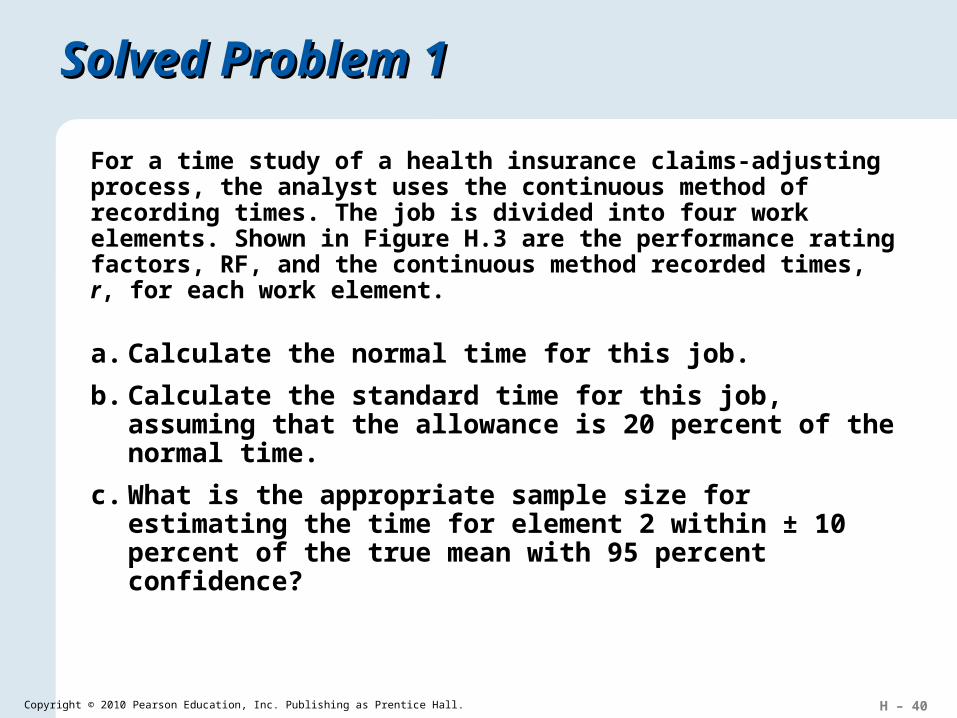
For a time study of a health insurance claims-adjusting process, the analyst uses the continuous method of recording times. The job is divided into four work elements. Shown in Figure H.3 are the performance rating factors, RF, and the continuous method recorded times, r, for each work element.
a. Calculate the normal time for this job.
b. Calculate the standard time for this job, assuming that the allowance is 20 percent of the normal time.
c. What is the appropriate sample size for estimating the time for element 2 within ± 10 percent of the true mean with 95 percent confidence?
H – 41Copyright © 2010 Pearson Education, Inc. Publishing as Prentice Hall.
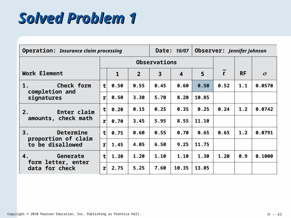
Operation: Insurance claim processing Date: 10/07 Observer: Jennifer Johnson
Work Element
Observations
t RF 1 2 3 4 5
1. Check form completion and signatures
t
r
2. Enter claim amounts, check math
t
r
3. Determine proportion of claim to be disallowed
t
r
4. Generate form letter, enter data for check
t
r
Solved Problem 1Solved Problem 1
0.50
0.50
0.52 1.1 0.0570
0.24 1.2 0.0742
0.65 1.2 0.0791
1.20 0.9 0.1000
0.20
0.70
0.75
1.45
1.30
2.75
0.55
3.30
0.15
3.45
0.60
4.05
1.20
5.25
0.45
5.70
0.25
5.95
0.55
6.50
1.10
7.60
0.60
8.20
0.35
8.55
0.70
9.25
1.10
10.35
0.50
10.85
0.25
11.10
0.65
11.75
1.30
13.05
H – 42Copyright © 2010 Pearson Education, Inc. Publishing as Prentice Hall.
Solved Problem 1Solved Problem 1
SOLUTION
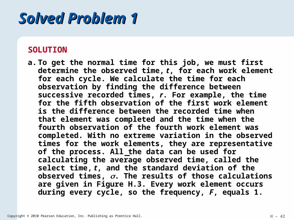
a. To get the normal time for this job, we must first determine the observed time, t, for each work element for each cycle. We calculate the time for each observation by finding the difference between successive recorded times, r. For example, the time for the fifth observation of the first work element is the difference between the recorded time when that element was completed and the time when the fourth observation of the fourth work element was completed. With no extreme variation in the observed times for the work elements, they are representative of the process. All the data can be used for calculating the average observed time, called the select time, t, and the standard deviation of the observed times, . The results of those calculations are given in Figure H.3. Every work element occurs during every cycle, so the frequency, F, equals 1.
H – 43Copyright © 2010 Pearson Education, Inc. Publishing as Prentice Hall.
Solved Problem 1Solved Problem 1
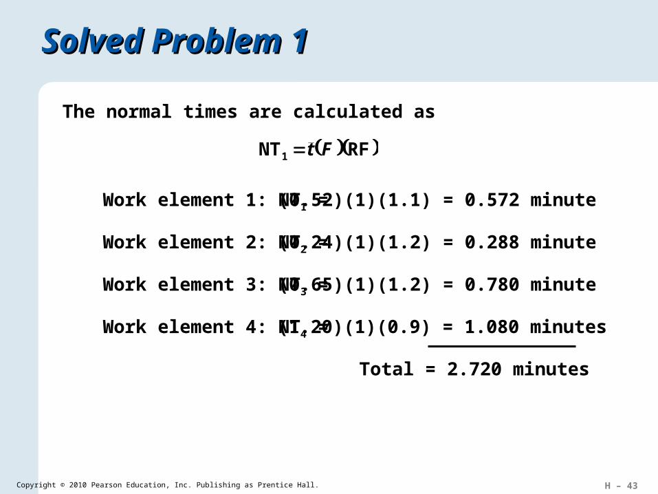
The normal times are calculated as
RFNT1 Ft
Work element 1: NT1 = (0.52)(1)(1.1) = 0.572 minute
Work element 2: NT2 = (0.24)(1)(1.2) = 0.288 minute
Work element 3: NT3 = (0.65)(1)(1.2) = 0.780 minute
Work element 4: NT4 = (1.20)(1)(0.9) = 1.080 minutes
Total = 2.720 minutes
H – 44Copyright © 2010 Pearson Education, Inc. Publishing as Prentice Hall.
Solved Problem 1Solved Problem 1
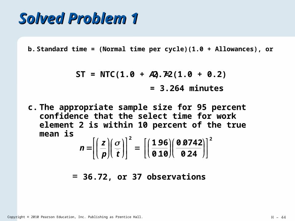
b. Standard time = (Normal time per cycle)(1.0 + Allowances), or
ST = NTC(1.0 + A) = 2.72(1.0 + 0.2)
= 3.264 minutes
c. The appropriate sample size for 95 percent confidence that the select time for work element 2 is within 10 percent of the true mean is
2
tpz
n 2
24007420
100961
..
.
.
= 36.72, or 37 observations
H – 45Copyright © 2010 Pearson Education, Inc. Publishing as Prentice Hall.
Solved Problem 2Solved Problem 2
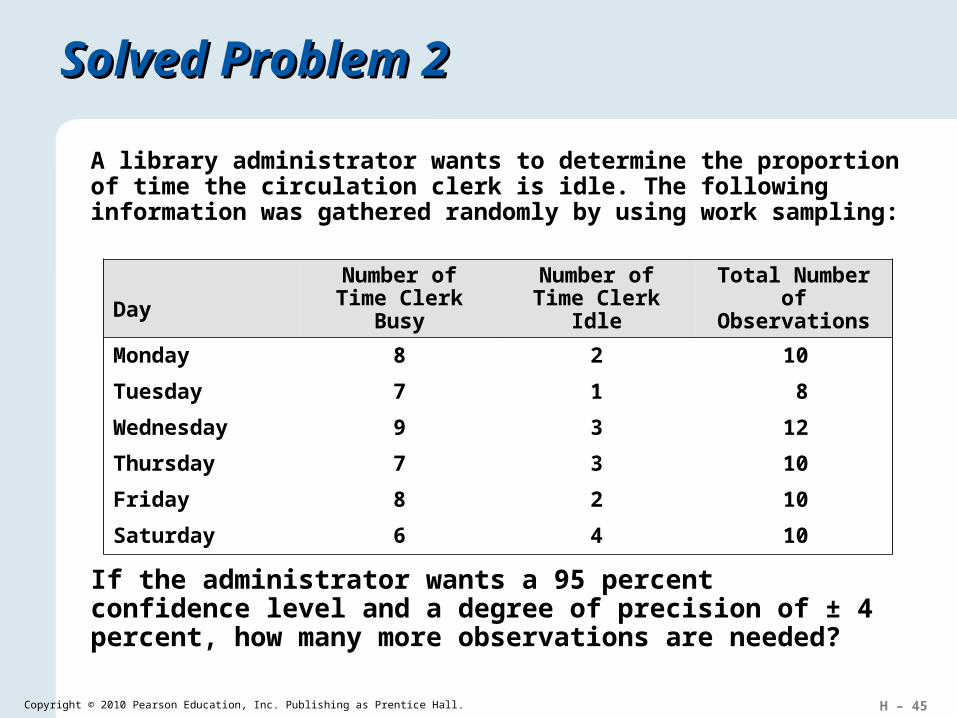
A library administrator wants to determine the proportion of time the circulation clerk is idle. The following information was gathered randomly by using work sampling:
DayNumber of Time
Clerk BusyNumber of Time
Clerk IdleTotal Number of
Observations
Monday 8 2 10
Tuesday 7 1 8
Wednesday 9 3 12
Thursday 7 3 10
Friday 8 2 10
Saturday 6 4 10
If the administrator wants a 95 percent confidence level and a degree of precision of ± 4 percent, how many more observations are needed?
H – 46Copyright © 2010 Pearson Education, Inc. Publishing as Prentice Hall.
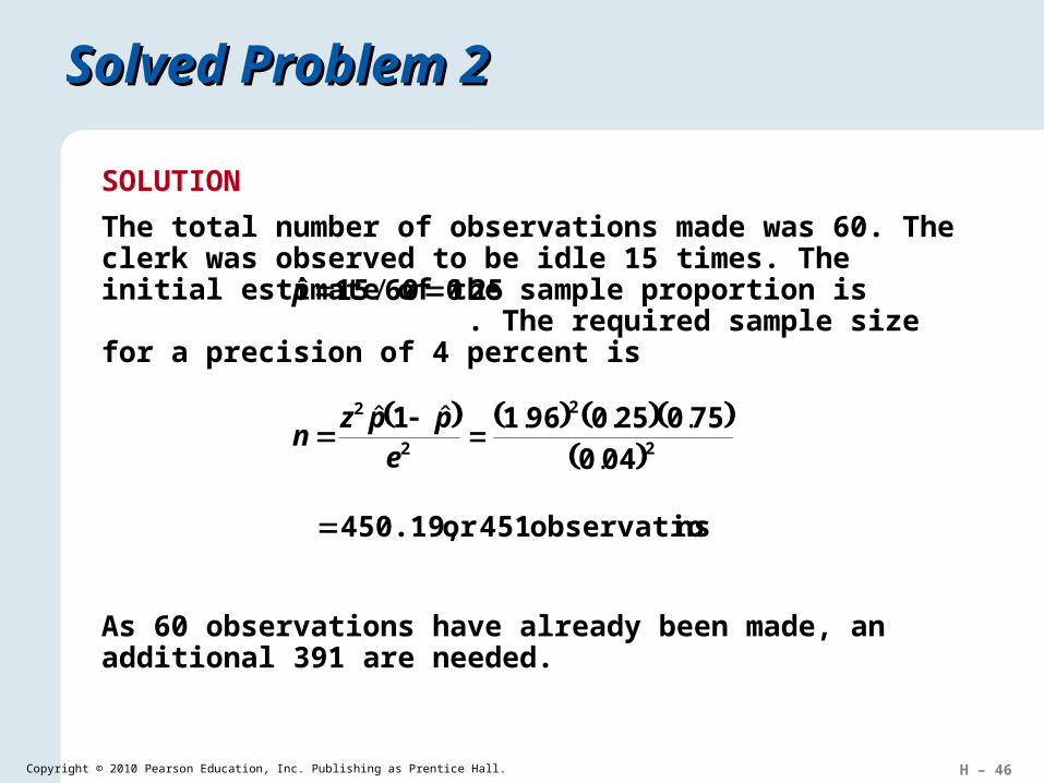
Solved Problem 2Solved Problem 2
2506015 ./ˆ p
SOLUTION
The total number of observations made was 60. The clerk was observed to be idle 15 times. The initial estimate of the sample proportion is . The required sample size for a precision of 4 percent is
2
2 1e
ppzn
ˆˆ 2
2
040
750250961
.
...
nsobservatio 451 or 450.19,
As 60 observations have already been made, an additional 391 are needed.

H – 47Copyright © 2010 Pearson Education, Inc. Publishing as Prentice Hall.