Embed Size (px)
Citation preview
1
ForecastingForecasting13
13 – 1Copyright © 2010 Pearson Education, Inc. Publishing as Prentice Hall.
For For Operations Management, 9eOperations Management, 9e by by Krajewski/Ritzman/Malhotra Krajewski/Ritzman/Malhotra © 2010 Pearson Education© 2010 Pearson Education
PowerPoint Slides PowerPoint Slides by Jeff Heylby Jeff Heyl
ForecastingForecasting
Forecasts are critical inputs to business plans, annual plans, and budgetsFinance, human resources, marketing, operations, and supply chain managers need forecasts to plan: output levels, purchases of services and materials, workforce and output schedules, inventories, and long-term capacitiesForecasts are made on many different variables
13 – 2Copyright © 2010 Pearson Education, Inc. Publishing as Prentice Hall.
Forecasts are important to managing both processes and managing supply chains
2
Demand PatternsDemand Patterns
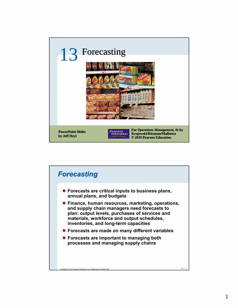
A time series is the repeated observations of demand for a service or product in their porder of occurrenceThere are five basic time series patterns
HorizontalTrendSeasonal
13 – 3Copyright © 2010 Pearson Education, Inc. Publishing as Prentice Hall.
SeasonalCyclicalRandom
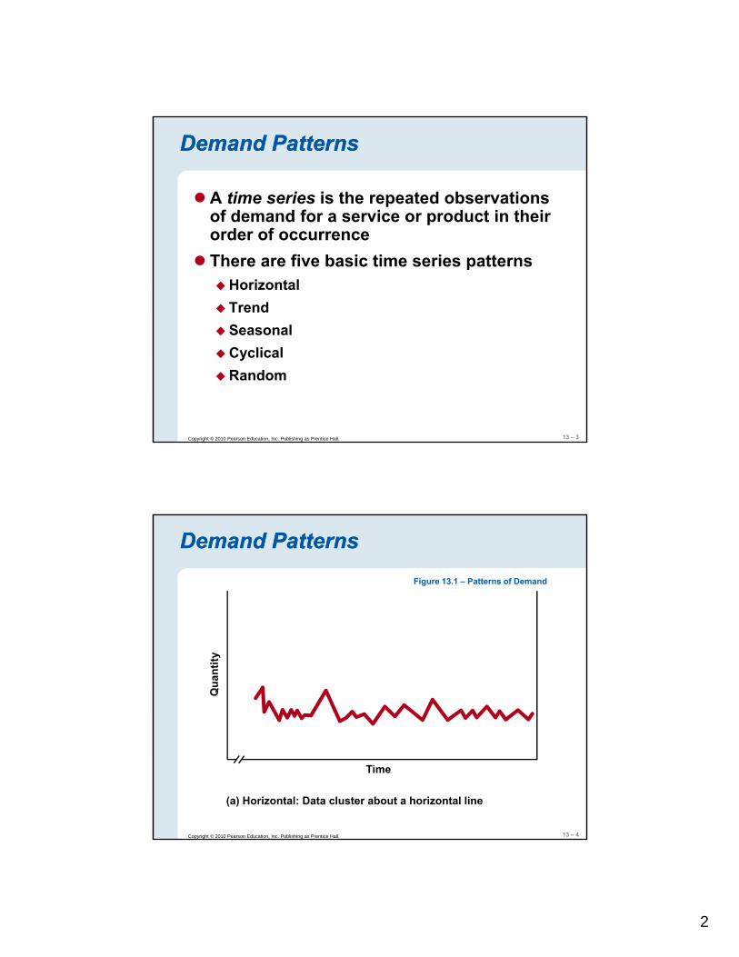
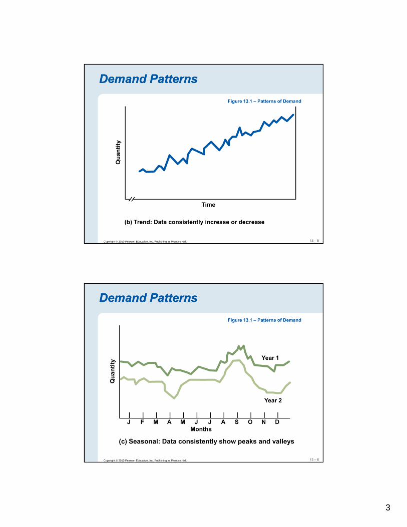
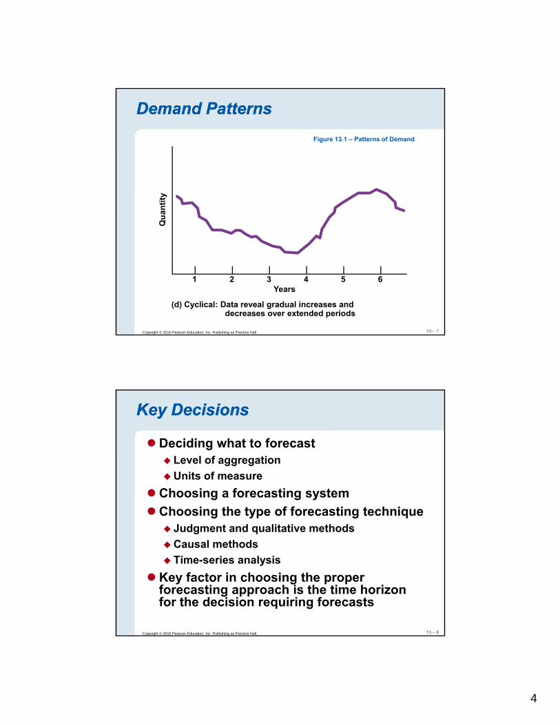
Demand PatternsDemand PatternsFigure 13.1 – Patterns of Demand
Qua
ntity
13 – 4Copyright © 2010 Pearson Education, Inc. Publishing as Prentice Hall.
Time
(a) Horizontal: Data cluster about a horizontal line
3
Demand PatternsDemand PatternsFigure 13.1 – Patterns of Demand
Qua
ntity
13 – 5Copyright © 2010 Pearson Education, Inc. Publishing as Prentice Hall.
Time
(b) Trend: Data consistently increase or decrease
Demand PatternsDemand PatternsFigure 13.1 – Patterns of Demand
Qua
ntity
Year 1
Year 2
13 – 6Copyright © 2010 Pearson Education, Inc. Publishing as Prentice Hall.
| | | | | | | | | | | |J F M A M J J A S O N D
Months
(c) Seasonal: Data consistently show peaks and valleys
4
Demand PatternsDemand PatternsFigure 13.1 – Patterns of Demand
Qua
ntity
13 – 7Copyright © 2010 Pearson Education, Inc. Publishing as Prentice Hall.
| | | | | |1 2 3 4 5 6
Years
(d) Cyclical: Data reveal gradual increases and decreases over extended periods
Key DecisionsKey Decisions
Deciding what to forecastLevel of aggregationU i fUnits of measure
Choosing a forecasting systemChoosing the type of forecasting technique
Judgment and qualitative methodsCausal methods
13 – 8Copyright © 2010 Pearson Education, Inc. Publishing as Prentice Hall.
Time-series analysisKey factor in choosing the proper forecasting approach is the time horizon for the decision requiring forecasts
5
Judgment MethodsJudgment Methods
Other methods (casual and time-series) require an adequate history file, which might not be availableJudgmental forecasts use contextual knowledge gained through experienceSalesforce estimatesExecutive opinion is a method in which opinions, experience, and technical knowledge of one or more managers are summarized to arrive at a
13 – 9Copyright © 2010 Pearson Education, Inc. Publishing as Prentice Hall.
gsingle forecastDelphi method
Judgment MethodsJudgment Methods
Market research is a systematic approach to determine external customer interest through d t th idata-gathering surveysDelphi method is a process of gaining consensus from a group of experts while maintaining their anonymityUseful when no historical data are available Can be used to develop long-range forecasts and
13 – 10Copyright © 2010 Pearson Education, Inc. Publishing as Prentice Hall.
p g gtechnological forecasting
6
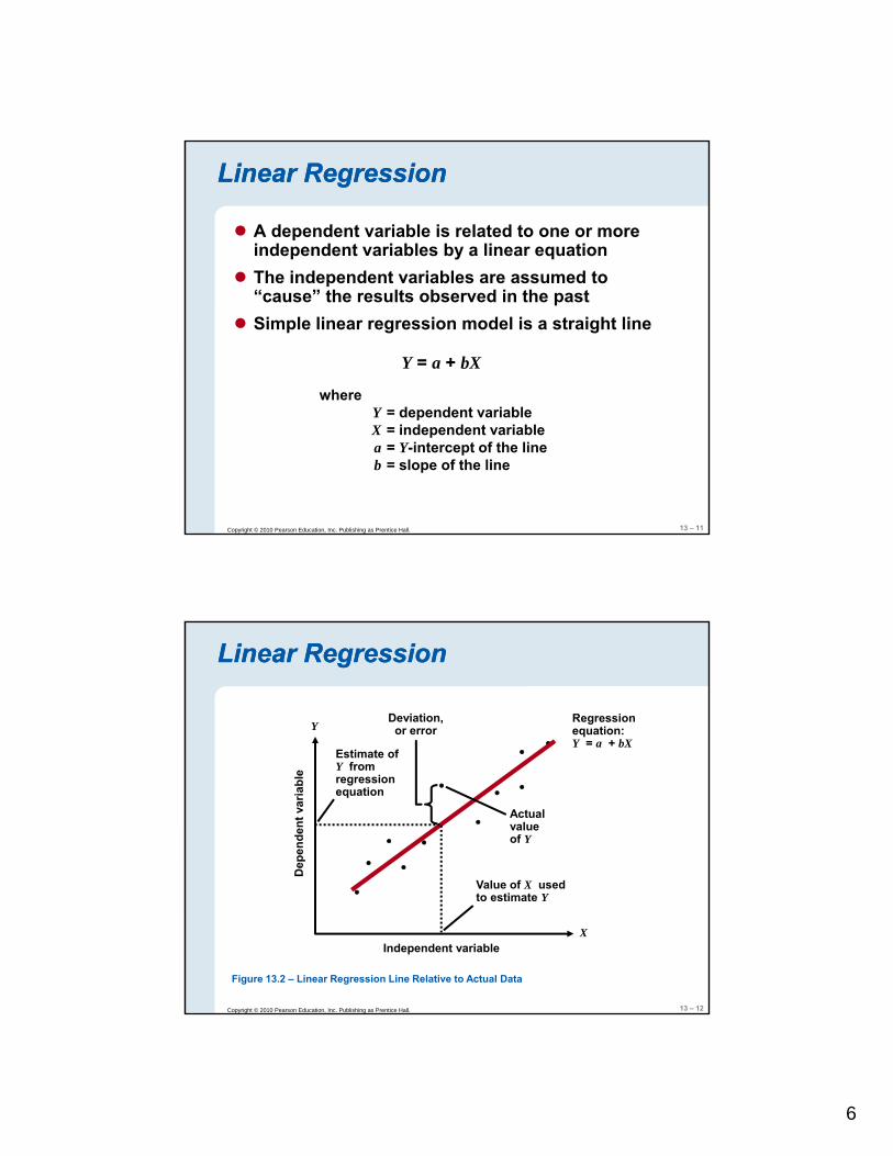
Linear RegressionLinear Regression
A dependent variable is related to one or more independent variables by a linear equationTh i d d t i bl d tThe independent variables are assumed to “cause” the results observed in the pastSimple linear regression model is a straight line
Y = a + bX
where
13 – 11Copyright © 2010 Pearson Education, Inc. Publishing as Prentice Hall.
Y = dependent variableX = independent variablea = Y-intercept of the lineb = slope of the line
Linear RegressionLinear Regression
Y
Estimate of
Regressionequation:Y = a + bX
Deviation,or error
Dep
ende
nt v
aria
ble
Estimate ofY fromregressionequation
Actualvalueof Y
Value of X used
13 – 12Copyright © 2010 Pearson Education, Inc. Publishing as Prentice Hall.
Independent variableX
Value of X usedto estimate Y
Figure 13.2 – Linear Regression Line Relative to Actual Data
7
Linear RegressionLinear Regression
The sample correlation coefficient, rMeasures the direction and strength of the relationship between the independent variable and the dependentbetween the independent variable and the dependent variable.The value of r can range from –1.00 ≤ r ≤ 1.00
The sample coefficient of determination, r2
Measures the amount of variation in the dependent variable about its mean that is explained by the regression line
13 – 13Copyright © 2010 Pearson Education, Inc. Publishing as Prentice Hall.
The values of r2 range from 0.00 ≤ r2 ≤ 1.00
The standard error of the estimate, syx
Measures how closely the data on the dependent variable cluster around the regression line
Using Linear RegressionUsing Linear Regression
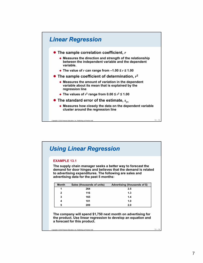
EXAMPLE 13.1The supply chain manager seeks a better way to forecast the demand for door hinges and believes that the demand is related gto advertising expenditures. The following are sales and advertising data for the past 5 months:
Month Sales (thousands of units) Advertising (thousands of $)1 264 2.52 116 1.33 165 1.44 101 1 0
13 – 14Copyright © 2010 Pearson Education, Inc. Publishing as Prentice Hall.
4 101 1.05 209 2.0
The company will spend $1,750 next month on advertising for the product. Use linear regression to develop an equation and a forecast for this product.
8
Using Linear RegressionUsing Linear Regression
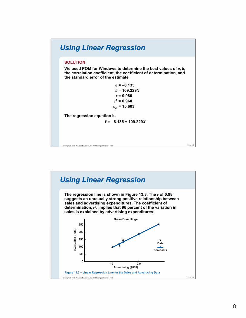
SOLUTIONWe used POM for Windows to determine the best values of a, b, the correlation coefficient, the coefficient of determination, and , ,the standard error of the estimate
a =b =r =
r2 =syx =
–8.135109.229X0.9800.96015.603
13 – 15Copyright © 2010 Pearson Education, Inc. Publishing as Prentice Hall.
The regression equation is Y = –8.135 + 109.229X
Using Linear RegressionUsing Linear Regression
The regression line is shown in Figure 13.3. The r of 0.98 suggests an unusually strong positive relationship between sales and advertising expenditures. The coefficient of determination 2 implies that 96 percent of the variation indetermination, r2, implies that 96 percent of the variation in sales is explained by advertising expenditures.
250 –
200 –
150 –
(000
uni
ts)
Brass Door Hinge
X
X
X
XData
13 – 16Copyright © 2010 Pearson Education, Inc. Publishing as Prentice Hall.
| |1.0 2.0
Advertising ($000)
100 –
50 –
0 –
Sale
s
XXData
Forecasts
Figure 13.3 – Linear Regression Line for the Sales and Advertising Data
9
Time Series MethodsTime Series Methods
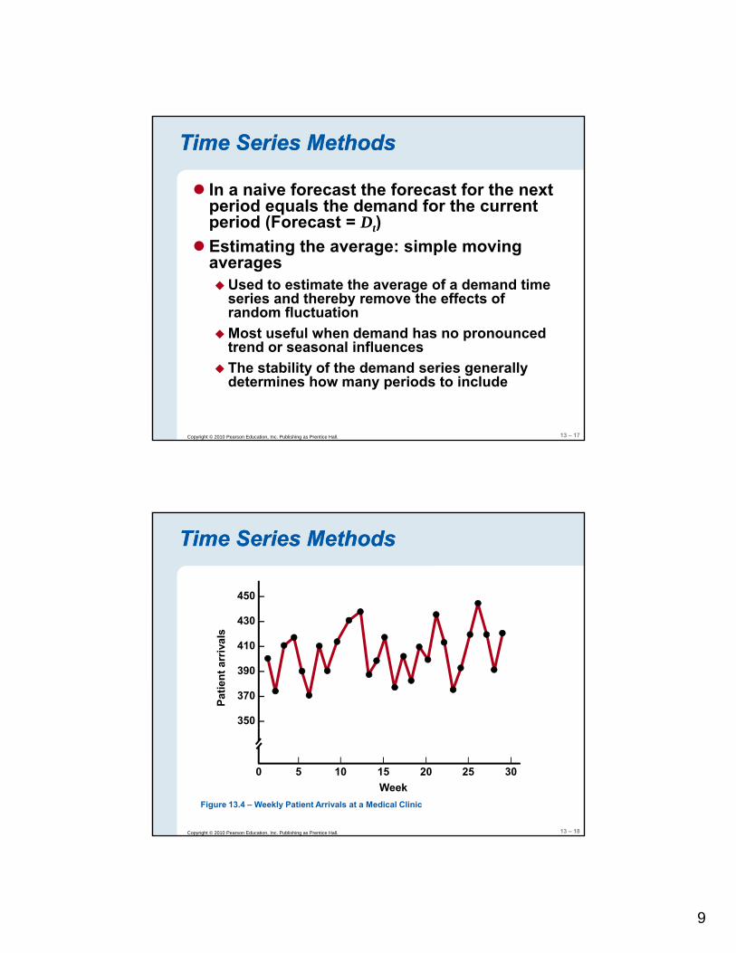
In a naive forecast the forecast for the next period equals the demand for the current period (Forecast = D )period (Forecast = Dt)Estimating the average: simple moving averages
Used to estimate the average of a demand time series and thereby remove the effects of random fluctuationMost useful when demand has no pronounced
13 – 17Copyright © 2010 Pearson Education, Inc. Publishing as Prentice Hall.
Most useful when demand has no pronounced trend or seasonal influencesThe stability of the demand series generally determines how many periods to include
450 –
430
Time Series MethodsTime Series Methods
430 –
410 –
390 –
370 –
350 –
Patie
nt a
rriv
als
13 – 18Copyright © 2010 Pearson Education, Inc. Publishing as Prentice Hall.
| | | | | |
0 5 10 15 20 25 30Week
Figure 13.4 – Weekly Patient Arrivals at a Medical Clinic
10
Simple Moving AveragesSimple Moving Averages
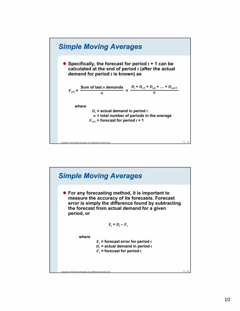
Specifically, the forecast for period t + 1 can be calculated at the end of period t (after the actual demand for period t is known) asdemand for period t is known) as
Ft+1 = =Sum of last n demands
nDt + Dt-1 + Dt-2 + … + Dt-n+1
n
where
13 – 19Copyright © 2010 Pearson Education, Inc. Publishing as Prentice Hall.
Dt = actual demand in period tn = total number of periods in the average
Ft+1 = forecast for period t + 1
Simple Moving AveragesSimple Moving Averages
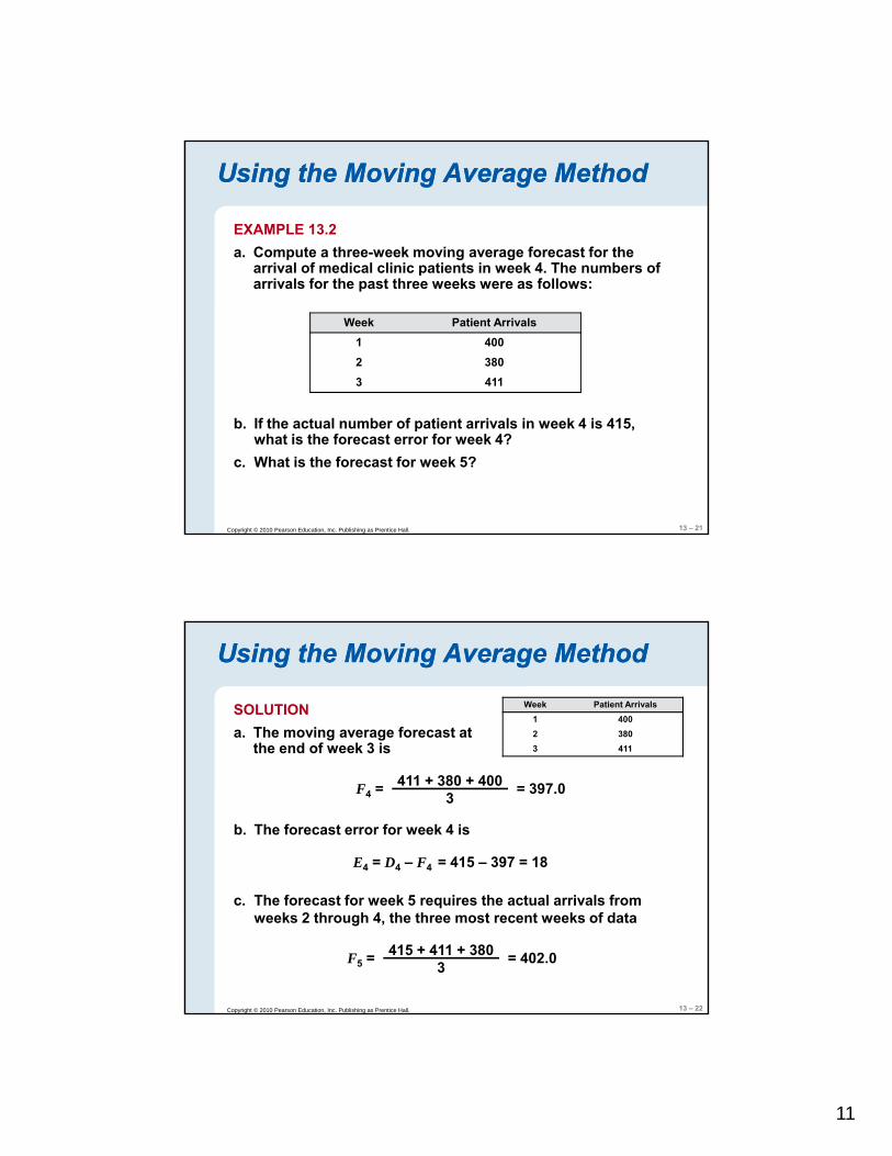
For any forecasting method, it is important to measure the accuracy of its forecasts. Forecast error is simply the difference found by subtractingerror is simply the difference found by subtracting the forecast from actual demand for a given period, or
where
Et = Dt – Ft
13 – 20Copyright © 2010 Pearson Education, Inc. Publishing as Prentice Hall.
whereEt = forecast error for period tDt = actual demand in period tFt = forecast for period t
11
Using the Moving Average MethodUsing the Moving Average Method
EXAMPLE 13.2a. Compute a three-week moving average forecast for the
arrival of medical clinic patients in week 4. The numbers ofarrival of medical clinic patients in week 4. The numbers of arrivals for the past three weeks were as follows:
Week Patient Arrivals1 4002 3803 411
13 – 21Copyright © 2010 Pearson Education, Inc. Publishing as Prentice Hall.
b. If the actual number of patient arrivals in week 4 is 415, what is the forecast error for week 4?
c. What is the forecast for week 5?
Using the Moving Average MethodUsing the Moving Average Method
SOLUTIONa. The moving average forecast at
the end of week 3 is
Week Patient Arrivals1 4002 3803 411the end of week 3 is
b. The forecast error for week 4 is
F4 = = 397.0411 + 380 + 4003
E4 = D4 – F4 = 415 – 397 = 18
13 – 22Copyright © 2010 Pearson Education, Inc. Publishing as Prentice Hall.
c. The forecast for week 5 requires the actual arrivals from weeks 2 through 4, the three most recent weeks of data
F5 = = 402.0415 + 411 + 3803
12
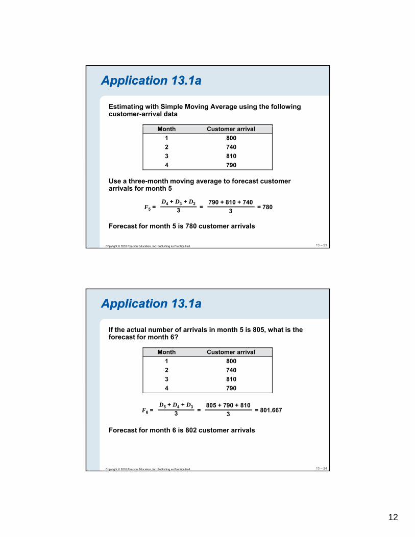
Application 13.1aApplication 13.1a
Estimating with Simple Moving Average using the following customer-arrival data
Month Customer arrival1 8002 7403 8104 790
Use a three-month moving average to forecast customer arrivals for month 5
13 – 23Copyright © 2010 Pearson Education, Inc. Publishing as Prentice Hall.
arrivals for month 5
F5 = = 780D4 + D3 + D2
3790 + 810 + 740
3=
Forecast for month 5 is 780 customer arrivals
Application 13.1aApplication 13.1a
If the actual number of arrivals in month 5 is 805, what is the forecast for month 6?
F = = 801 667D5 + D4 + D3 805 + 790 + 810
=
Month Customer arrival1 8002 7403 8104 790
13 – 24Copyright © 2010 Pearson Education, Inc. Publishing as Prentice Hall.
F6 = = 801.6673 3=
Forecast for month 6 is 802 customer arrivals
13
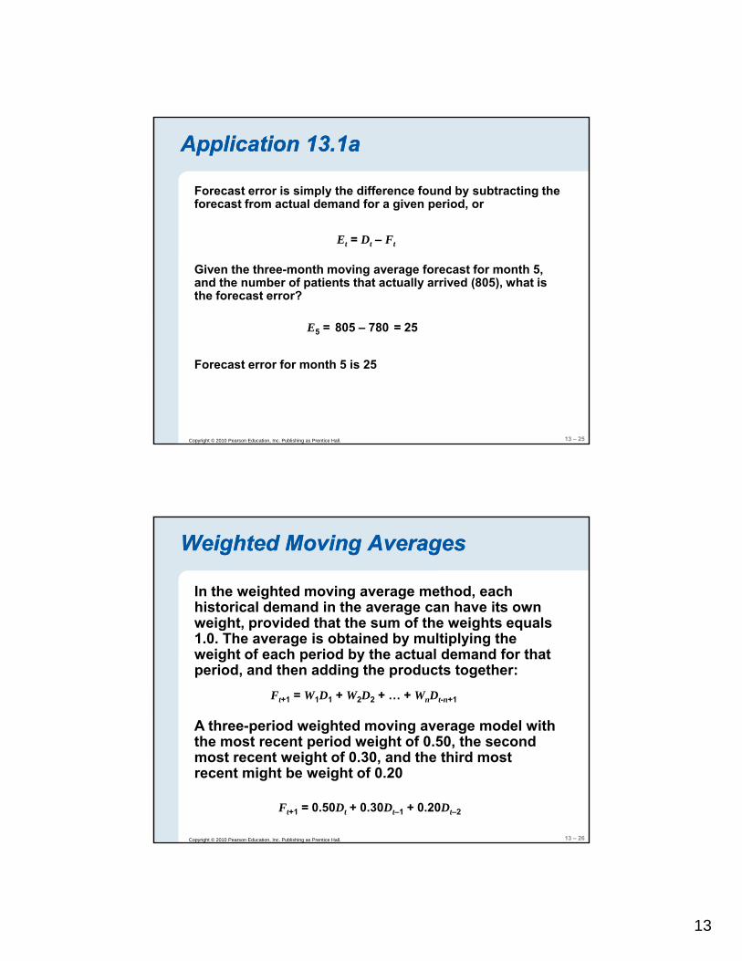
Application 13.1aApplication 13.1a
Forecast error is simply the difference found by subtracting the forecast from actual demand for a given period, or
Given the three-month moving average forecast for month 5, and the number of patients that actually arrived (805), what is the forecast error?
Et = Dt – Ft
E5 = 805 – 780 = 25
13 – 25Copyright © 2010 Pearson Education, Inc. Publishing as Prentice Hall.
Forecast error for month 5 is 25
In the weighted moving average method, each historical demand in the average can have its own weight provided that the sum of the weights equals
Weighted Moving AveragesWeighted Moving Averages
weight, provided that the sum of the weights equals 1.0. The average is obtained by multiplying the weight of each period by the actual demand for that period, and then adding the products together:
Ft+1 = W1D1 + W2D2 + … + WnDt-n+1
A three-period weighted moving average model with
13 – 26Copyright © 2010 Pearson Education, Inc. Publishing as Prentice Hall.
the most recent period weight of 0.50, the second most recent weight of 0.30, and the third most recent might be weight of 0.20
Ft+1 = 0.50Dt + 0.30Dt–1 + 0.20Dt–2
14
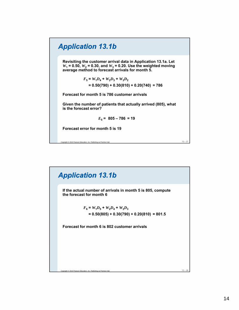
Application 13.1bApplication 13.1b
Revisiting the customer arrival data in Application 13.1a. Let W1 = 0.50, W2 = 0.30, and W3 = 0.20. Use the weighted moving average method to forecast arrivals for month 5.
= 0.50(790) + 0.30(810) + 0.20(740)F5 = W1D4 + W2D3 + W3D2
= 786
Forecast for month 5 is 786 customer arrivals
Given the number of patients that actually arrived (805), what is the forecast error?
13 – 27Copyright © 2010 Pearson Education, Inc. Publishing as Prentice Hall.
is the forecast error?
Forecast error for month 5 is 19
E5 = 805 – 786 = 19
Application 13.1bApplication 13.1b
If the actual number of arrivals in month 5 is 805, compute the forecast for month 6
= 0.50(805) + 0.30(790) + 0.20(810)F6 = W1D5 + W2D4 + W3D3
= 801.5
Forecast for month 6 is 802 customer arrivals
13 – 28Copyright © 2010 Pearson Education, Inc. Publishing as Prentice Hall.
15
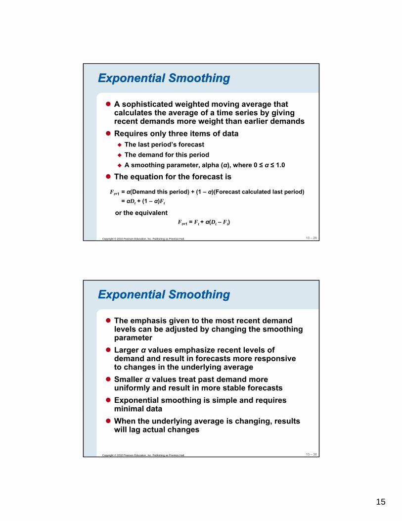
Exponential SmoothingExponential Smoothing
A sophisticated weighted moving average that calculates the average of a time series by giving recent demands more weight than earlier demandsrecent demands more weight than earlier demandsRequires only three items of data
The last period’s forecastThe demand for this periodA smoothing parameter, alpha (α), where 0 ≤ α ≤ 1.0
The equation for the forecast is
13 – 29Copyright © 2010 Pearson Education, Inc. Publishing as Prentice Hall.
Ft+1 = α(Demand this period) + (1 – α)(Forecast calculated last period)= αDt + (1 – α)Ft
Ft+1 = Ft + α(Dt – Ft)or the equivalent
Exponential SmoothingExponential Smoothing
The emphasis given to the most recent demand levels can be adjusted by changing the smoothing parameterparameterLarger α values emphasize recent levels of demand and result in forecasts more responsive to changes in the underlying averageSmaller α values treat past demand more uniformly and result in more stable forecastsE ti l thi i i l d i
13 – 30Copyright © 2010 Pearson Education, Inc. Publishing as Prentice Hall.
Exponential smoothing is simple and requires minimal dataWhen the underlying average is changing, results will lag actual changes
16
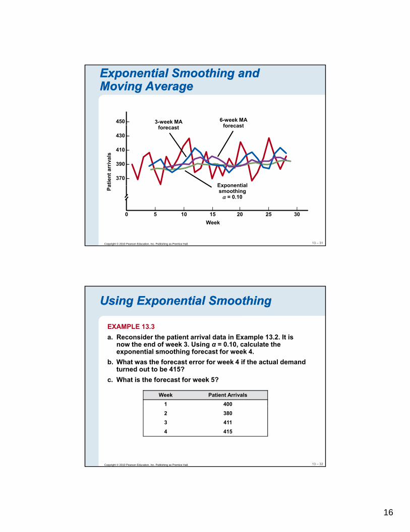
450 – 3-week MA 6-week MAforecast
Exponential Smoothing and Exponential Smoothing and Moving AverageMoving Average
430 –
410 –
390 –
370 –
atie
nt a
rriv
als
forecast forecast
Exponential
13 – 31Copyright © 2010 Pearson Education, Inc. Publishing as Prentice Hall.
Pa
Week
| | | | | |0 5 10 15 20 25 30
Exponential smoothingα = 0.10
Using Exponential SmoothingUsing Exponential Smoothing
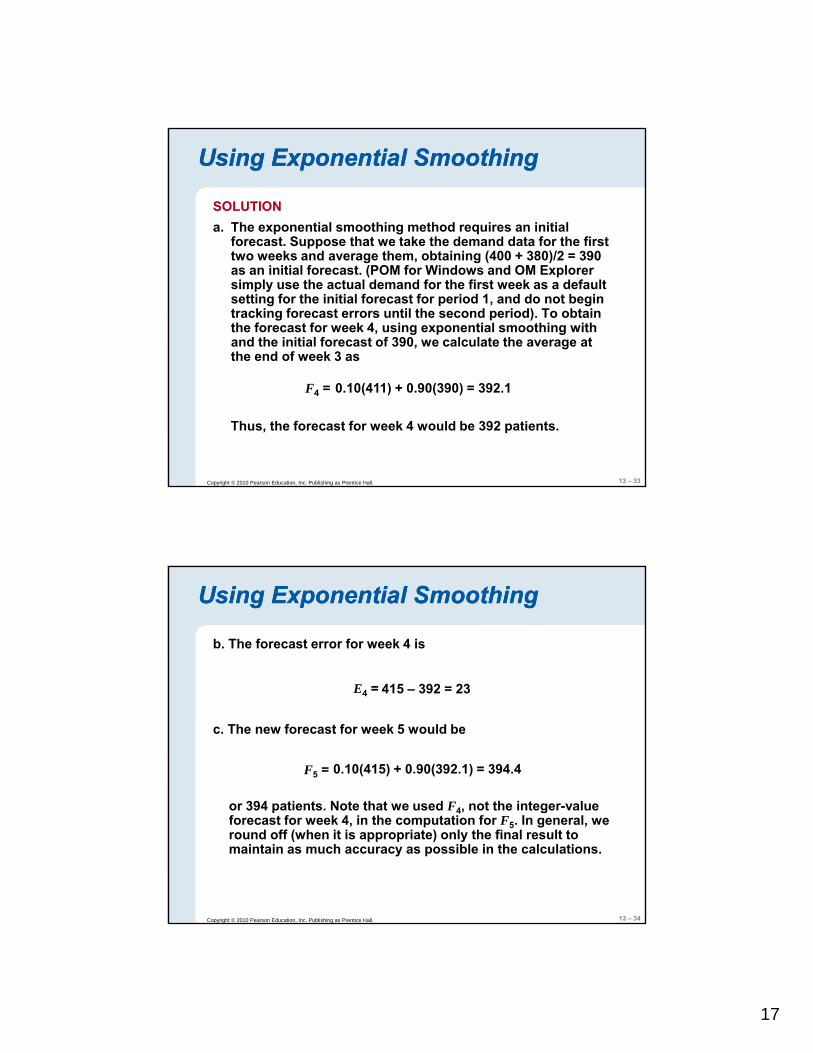
EXAMPLE 13.3a. Reconsider the patient arrival data in Example 13.2. It is
now the end of week 3. Using α = 0.10, calculate thenow the end of week 3. Using α 0.10, calculate the exponential smoothing forecast for week 4.
Week Patient Arrivals1 400
b. What was the forecast error for week 4 if the actual demand turned out to be 415?
c. What is the forecast for week 5?
13 – 32Copyright © 2010 Pearson Education, Inc. Publishing as Prentice Hall.
2 3803 4114 415
17
Using Exponential SmoothingUsing Exponential Smoothing
SOLUTIONa. The exponential smoothing method requires an initial
forecast. Suppose that we take the demand data for the first pptwo weeks and average them, obtaining (400 + 380)/2 = 390 as an initial forecast. (POM for Windows and OM Explorer simply use the actual demand for the first week as a default setting for the initial forecast for period 1, and do not begin tracking forecast errors until the second period). To obtain the forecast for week 4, using exponential smoothing with and the initial forecast of 390, we calculate the average at the end of week 3 as
13 – 33Copyright © 2010 Pearson Education, Inc. Publishing as Prentice Hall.
F4 =
Thus, the forecast for week 4 would be 392 patients.
0.10(411) + 0.90(390) = 392.1
Using Exponential SmoothingUsing Exponential Smoothing
b. The forecast error for week 4 is
E 415 392 23
c. The new forecast for week 5 would be
E4 =
F5 =
or 394 patients Note that we used F not the integer value
415 – 392 = 23
0.10(415) + 0.90(392.1) = 394.4
13 – 34Copyright © 2010 Pearson Education, Inc. Publishing as Prentice Hall.
or 394 patients. Note that we used F4, not the integer-value forecast for week 4, in the computation for F5. In general, we round off (when it is appropriate) only the final result to maintain as much accuracy as possible in the calculations.
18
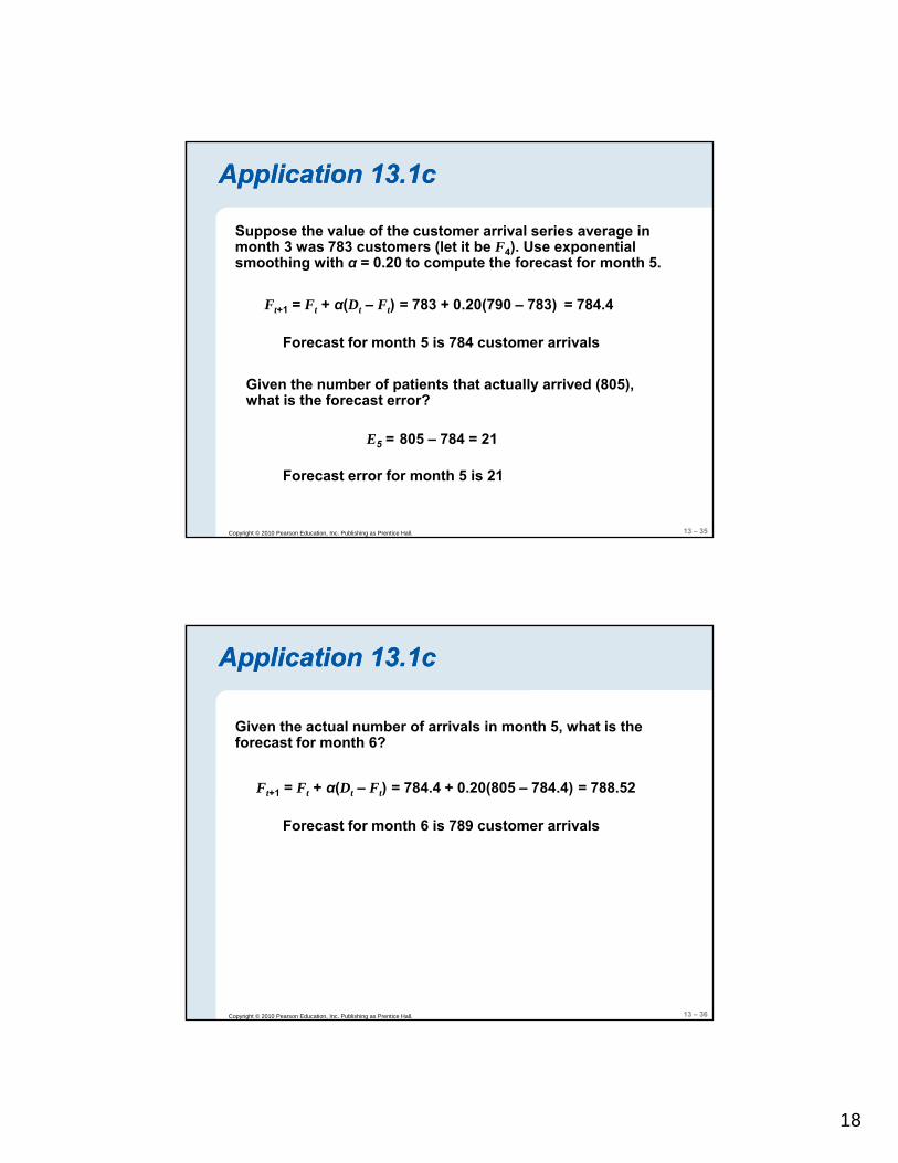
Application 13.1cApplication 13.1c
Suppose the value of the customer arrival series average in month 3 was 783 customers (let it be F4). Use exponential smoothing with α = 0.20 to compute the forecast for month 5.
Ft+1 = Ft + α(Dt – Ft) = 783 + 0.20(790 – 783) = 784.4
Forecast for month 5 is 784 customer arrivals
Given the number of patients that actually arrived (805), what is the forecast error?
13 – 35Copyright © 2010 Pearson Education, Inc. Publishing as Prentice Hall.
E5 =
Forecast error for month 5 is 21
805 – 784 = 21
Application 13.1cApplication 13.1c
Given the actual number of arrivals in month 5, what is the forecast for month 6?
Ft+1 = Ft + α(Dt – Ft) = 784.4 + 0.20(805 – 784.4) = 788.52
Forecast for month 6 is 789 customer arrivals
13 – 36Copyright © 2010 Pearson Education, Inc. Publishing as Prentice Hall.
19
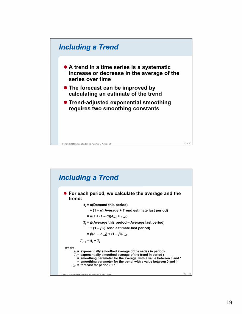
Including a TrendIncluding a Trend
A trend in a time series is a systematic increase or decrease in the average of theincrease or decrease in the average of the series over timeThe forecast can be improved by calculating an estimate of the trendTrend-adjusted exponential smoothing requires two smoothing constants
13 – 37Copyright © 2010 Pearson Education, Inc. Publishing as Prentice Hall.
requires two smoothing constants
Including a TrendIncluding a Trend
For each period, we calculate the average and the trend:
A = α(Demand this period)At = α(Demand this period) + (1 – α)(Average + Trend estimate last period)
= αDt + (1 – α)(At–1 + Tt–1)
Tt = β(Average this period – Average last period)+ (1 – β)(Trend estimate last period)
= β(At – At–1) + (1 – β)Tt–1
F A + T
13 – 38Copyright © 2010 Pearson Education, Inc. Publishing as Prentice Hall.
Ft+1 = At + Tt
whereAt = exponentially smoothed average of the series in period tTt = exponentially smoothed average of the trend in period t
= smoothing parameter for the average, with a value between 0 and 1= smoothing parameter for the trend, with a value between 0 and 1
Ft+1 = forecast for period t + 1
20
Using TrendUsing Trend--Adjusted Exponential Adjusted Exponential SmoothingSmoothing
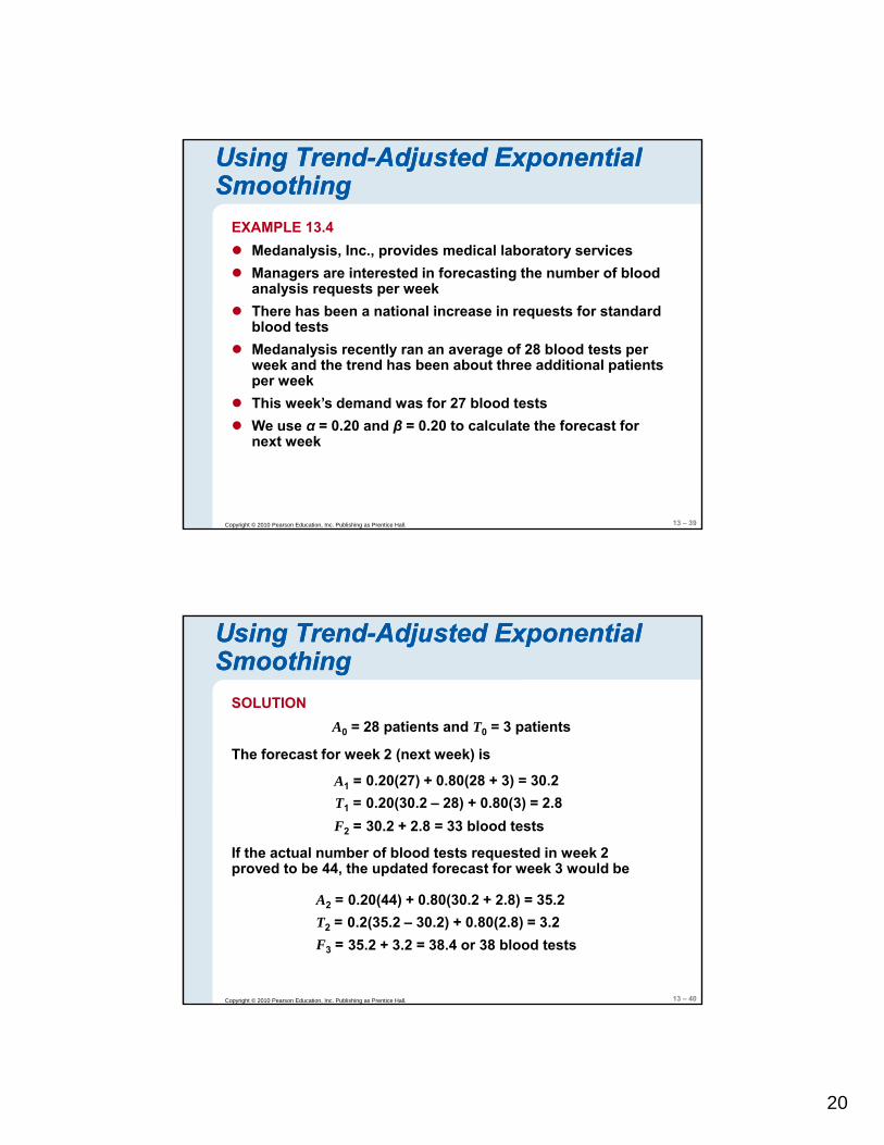
EXAMPLE 13.4Medanalysis, Inc., provides medical laboratory services M i t t d i f ti th b f bl dManagers are interested in forecasting the number of blood analysis requests per weekThere has been a national increase in requests for standard blood testsMedanalysis recently ran an average of 28 blood tests per week and the trend has been about three additional patients per weekThi k’ d d f 27 bl d t t
13 – 39Copyright © 2010 Pearson Education, Inc. Publishing as Prentice Hall.
This week’s demand was for 27 blood testsWe use α = 0.20 and β = 0.20 to calculate the forecast for next week
Using TrendUsing Trend--Adjusted Exponential Adjusted Exponential SmoothingSmoothing
SOLUTIONA0 = 28 patients and T0 = 3 patients
30.2 + 2.8 = 33 blood tests
If the actual number of blood tests requested in week 2 proved to be 44, the updated forecast for week 3 would be
The forecast for week 2 (next week) is
A1 =T1 =F2 =
0.20(27) + 0.80(28 + 3) = 30.20.20(30.2 – 28) + 0.80(3) = 2.8
13 – 40Copyright © 2010 Pearson Education, Inc. Publishing as Prentice Hall.
p , p
A2 =
F3 = 35.2 + 3.2 = 38.4 or 38 blood tests0.2(35.2 – 30.2) + 0.80(2.8) = 3.20.20(44) + 0.80(30.2 + 2.8) = 35.2
T2 =
21
Using TrendUsing Trend--Adjusted Exponential Adjusted Exponential SmoothingSmoothing
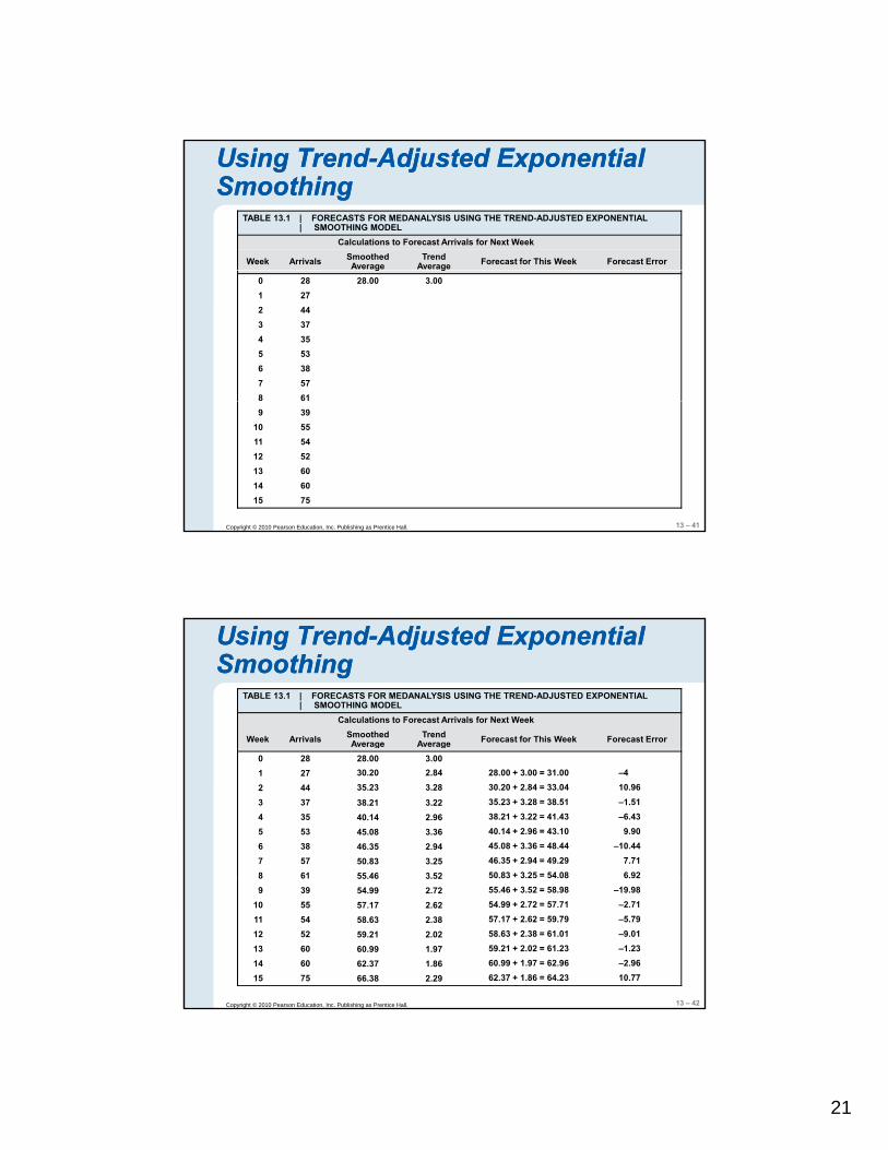
TABLE 13.1 | FORECASTS FOR MEDANALYSIS USING THE TREND-ADJUSTED EXPONENTIAL| SMOOTHING MODEL
Calculations to Forecast Arrivals for Next Week
Week Arrivals Smoothed Average
Trend Average Forecast for This Week Forecast Errorg g
0 28 28.00 3.001 272 443 374 355 536 387 578 61
13 – 41Copyright © 2010 Pearson Education, Inc. Publishing as Prentice Hall.
9 3910 5511 5412 5213 6014 6015 75
Using TrendUsing Trend--Adjusted Exponential Adjusted Exponential SmoothingSmoothing
TABLE 13.1 | FORECASTS FOR MEDANALYSIS USING THE TREND-ADJUSTED EXPONENTIAL| SMOOTHING MODEL
Calculations to Forecast Arrivals for Next Week
Week Arrivals Smoothed Average
Trend Average Forecast for This Week Forecast Error
30.20 + 2.84 = 33.04–430.20
35.232.843.28
28.00 + 3.00 = 31.00
35.23 + 3.28 = 38.5138.21 + 3.22 = 41.4340.14 + 2.96 = 43.1045.08 + 3.36 = 48.4446.35 + 2.94 = 49.2950.83 + 3.25 = 54.08
10.96–1.51–6.43
9.90–10.44
7.716.92
38.2140.1445.0846.3550.8355.46
3.222.963.362.943.253.52
g g0 28 28.00 3.001 272 443 374 355 536 387 578 61
13 – 42Copyright © 2010 Pearson Education, Inc. Publishing as Prentice Hall.
55.46 + 3.52 = 58.9854.99 + 2.72 = 57.7157.17 + 2.62 = 59.7958.63 + 2.38 = 61.0159.21 + 2.02 = 61.2360.99 + 1.97 = 62.9662.37 + 1.86 = 64.23
–19.98–2.71–5.79–9.01–1.23–2.9610.77
55 654.9957.1758.6359.2160.9962.3766.38
3 52.722.622.382.021.971.862.29
9 3910 5511 5412 5213 6014 6015 75
22
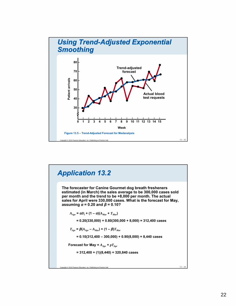
80 –
70 –Trend-adjusted
forecast
Using TrendUsing Trend--Adjusted Exponential Adjusted Exponential SmoothingSmoothing
70
60 –
50 –
40 –
30
Patie
nt a
rriv
als
Actual blood test requests
forecast
13 – 43Copyright © 2010 Pearson Education, Inc. Publishing as Prentice Hall.
| | | | | | | | | | | | | | | |0 1 2 3 4 5 6 7 8 9 10 11 12 13 14 15
30 –
WeekFigure 13.5 – Trend-Adjusted Forecast for Medanalysis
Application 13.2Application 13.2
The forecaster for Canine Gourmet dog breath fresheners estimated (in March) the sales average to be 300,000 cases sold per month and the trend to be +8,000 per month. The actual
l f A il 330 000 Wh t i th f t f Msales for April were 330,000 cases. What is the forecast for May, assuming α = 0.20 and β = 0.10?
AApr = αDt + (1 – α)(AMar + TMar)
TApr = β(AApr – AMar) + (1 – β)TMar
= 0.20(330,000) + 0.80(300,000 + 8,000) = 312,400 cases
13 – 44Copyright © 2010 Pearson Education, Inc. Publishing as Prentice Hall.
Forecast for May = AApr + pTApr
= 0.10(312,400 – 300,000) + 0.90(8,000) = 8,440 cases
= 312,400 + (1)(8,440) = 320,840 cases
23
Application 13.2Application 13.2
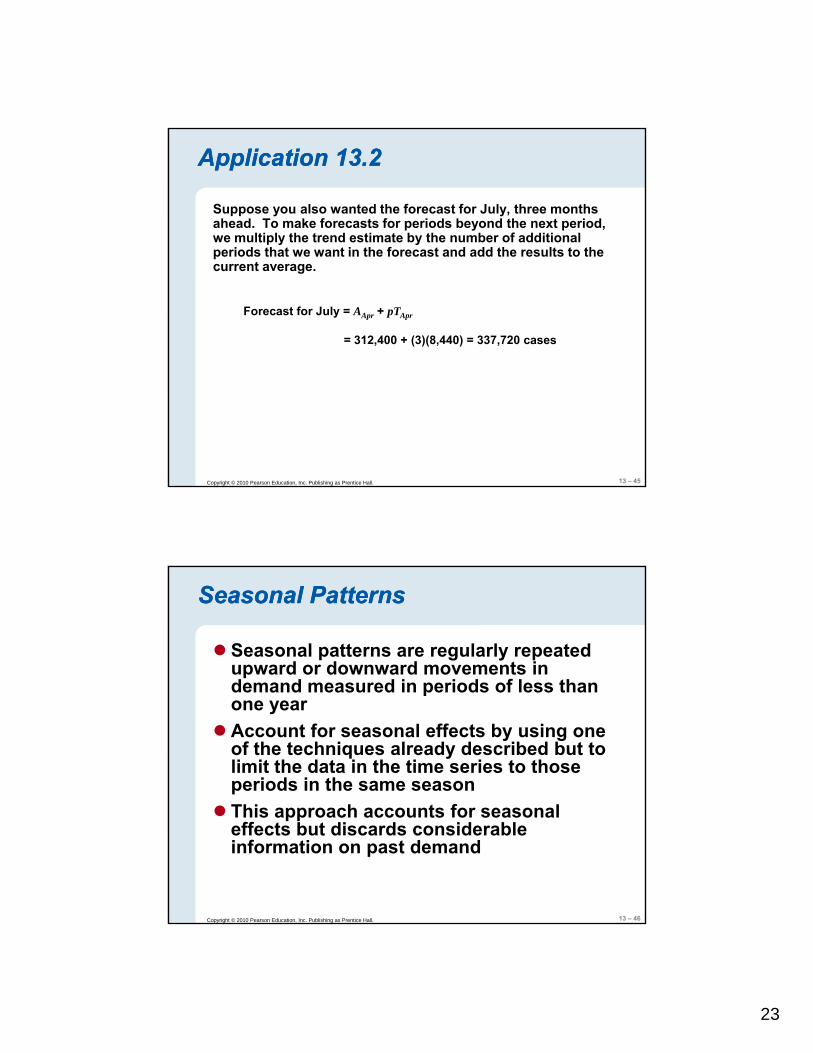
Suppose you also wanted the forecast for July, three months ahead. To make forecasts for periods beyond the next period, we multiply the trend estimate by the number of additional
i d th t t i th f t d dd th lt t thperiods that we want in the forecast and add the results to the current average.
Forecast for July = AApr + pTApr
= 312,400 + (3)(8,440) = 337,720 cases
13 – 45Copyright © 2010 Pearson Education, Inc. Publishing as Prentice Hall.
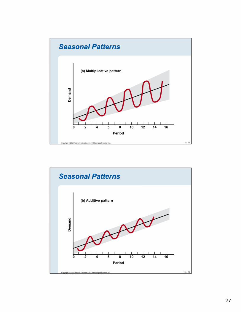
Seasonal PatternsSeasonal Patterns
Seasonal patterns are regularly repeated upward or downward movements in demand measured in periods of less thandemand measured in periods of less than one year Account for seasonal effects by using one of the techniques already described but to limit the data in the time series to those periods in the same seasonThi h t f l
13 – 46Copyright © 2010 Pearson Education, Inc. Publishing as Prentice Hall.
This approach accounts for seasonal effects but discards considerable information on past demand
24
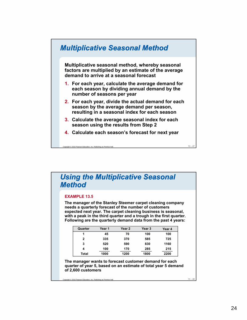
Multiplicative Seasonal MethodMultiplicative Seasonal Method
Multiplicative seasonal method, whereby seasonal factors are multiplied by an estimate of the average demand to arrive at a seasonal forecast1. For each year, calculate the average demand for
each season by dividing annual demand by the number of seasons per year
2. For each year, divide the actual demand for each season by the average demand per season, resulting in a seasonal index for each season
demand to arrive at a seasonal forecast
13 – 47Copyright © 2010 Pearson Education, Inc. Publishing as Prentice Hall.
resulting in a seasonal index for each season3. Calculate the average seasonal index for each
season using the results from Step 24. Calculate each season’s forecast for next year
Using the Multiplicative Seasonal Using the Multiplicative Seasonal Method Method
EXAMPLE 13.5The manager of the Stanley Steemer carpet cleaning company needs a quarterly forecast of the number of customersneeds a quarterly forecast of the number of customers expected next year. The carpet cleaning business is seasonal, with a peak in the third quarter and a trough in the first quarter. Following are the quarterly demand data from the past 4 years:
Quarter Year 1 Year 2 Year 3 Year 41 45 70 100 1002 335 370 585 7253 520 590 830 1160
13 – 48Copyright © 2010 Pearson Education, Inc. Publishing as Prentice Hall.
The manager wants to forecast customer demand for each quarter of year 5, based on an estimate of total year 5 demand of 2,600 customers
3 520 590 830 11604 100 170 285 215
Total 1000 1200 1800 2200
25
Using the Multiplicative Seasonal Using the Multiplicative Seasonal Method Method
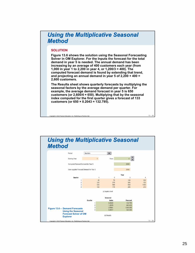
SOLUTIONFigure 13.6 shows the solution using the Seasonal Forecasting Solver in OM Explorer. For the Inputs the forecast for the totalSolver in OM Explorer. For the Inputs the forecast for the total demand in year 5 is needed. The annual demand has been increasing by an average of 400 customers each year (from 1,000 in year 1 to 2,200 in year 4, or 1,200/3 = 400). The computed forecast demand is found by extending that trend, and projecting an annual demand in year 5 of 2,200 + 400 = 2,600 customers. The Results sheet shows quarterly forecasts by multiplying the seasonal factors by the average demand per quarter For
13 – 49Copyright © 2010 Pearson Education, Inc. Publishing as Prentice Hall.
seasonal factors by the average demand per quarter. For example, the average demand forecast in year 5 is 650 customers (or 2,600/4 = 650). Multiplying that by the seasonal index computed for the first quarter gives a forecast of 133 customers (or 650 × 0.2043 = 132.795).
Using the Multiplicative Seasonal Using the Multiplicative Seasonal Method Method
13 – 50Copyright © 2010 Pearson Education, Inc. Publishing as Prentice Hall.
Figure 13.6 – Demand Forecasts Using the Seasonal Forecast Solver of OM Explorer
26
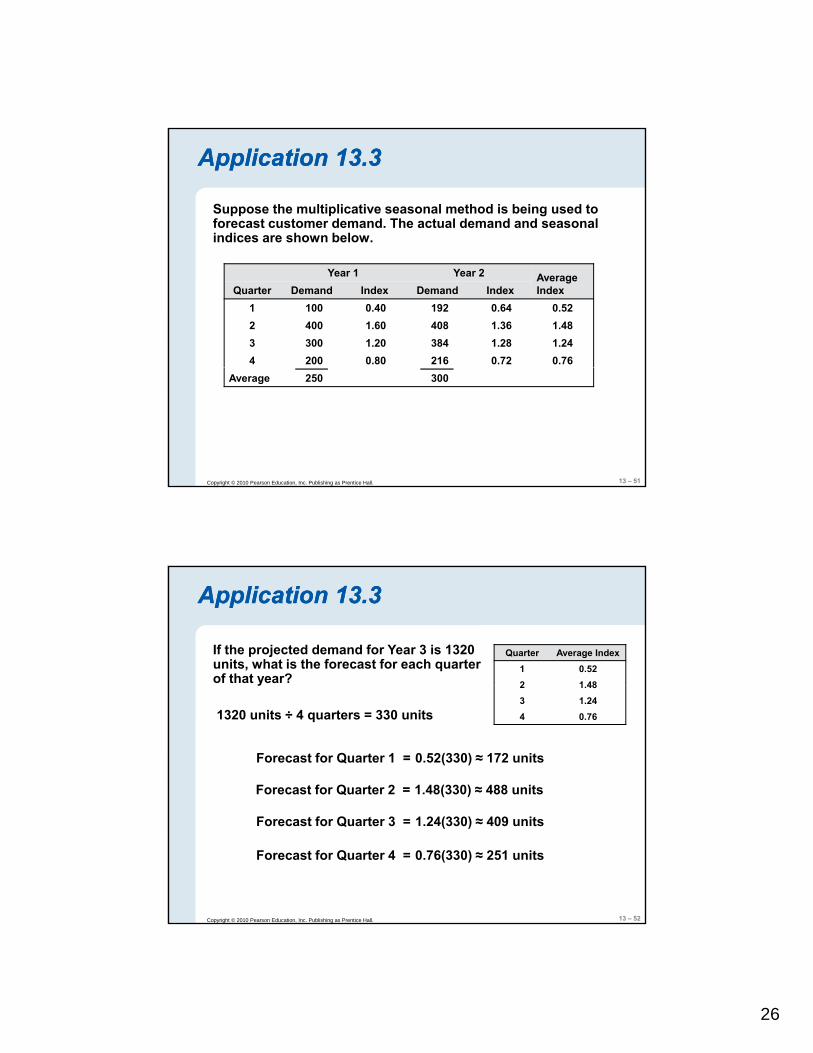
Application 13.3Application 13.3
Suppose the multiplicative seasonal method is being used to forecast customer demand. The actual demand and seasonal indices are shown below.
Year 1 Year 2 Average IndexQuarter Demand Index Demand Index
1 100 0.40 192 0.64 0.522 400 1.60 408 1.36 1.483 300 1.20 384 1.28 1.244 200 0.80 216 0.72 0.76
13 – 51Copyright © 2010 Pearson Education, Inc. Publishing as Prentice Hall.
Average 250 300
Application 13.3Application 13.3
Quarter Average Index1 0.522 1 48
If the projected demand for Year 3 is 1320 units, what is the forecast for each quarter of that year?
1320 units ÷ 4 quarters = 330 units
2 1.483 1.244 0.76
y
Forecast for Quarter 1 =
Forecast for Quarter 2 =
0.52(330) ≈ 172 units
1.48(330) ≈ 488 units
13 – 52Copyright © 2010 Pearson Education, Inc. Publishing as Prentice Hall.
Forecast for Quarter 3 =
Forecast for Quarter 4 =
1.24(330) ≈ 409 units
0.76(330) ≈ 251 units
27
(a) Multiplicative pattern
Seasonal PatternsSeasonal Patterns
Dem
and
13 – 53Copyright © 2010 Pearson Education, Inc. Publishing as Prentice Hall.
Period
| | | | | | | | | | | | | | | |0 2 4 5 8 10 12 14 16
Seasonal PatternsSeasonal Patterns
(b) Additive pattern
Dem
and
13 – 54Copyright © 2010 Pearson Education, Inc. Publishing as Prentice Hall.
Period
| | | | | | | | | | | | | | | |0 2 4 5 8 10 12 14 16
28
Choosing a TimeChoosing a Time--Series MethodSeries Method
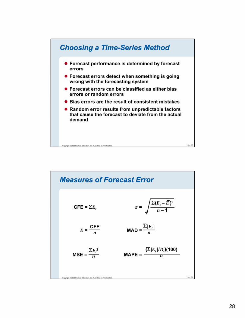
Forecast performance is determined by forecast errorsF t d t t h thi i iForecast errors detect when something is going wrong with the forecasting systemForecast errors can be classified as either bias errors or random errorsBias errors are the result of consistent mistakesRandom error results from unpredictable factors
13 – 55Copyright © 2010 Pearson Education, Inc. Publishing as Prentice Hall.
pthat cause the forecast to deviate from the actual demand
CFE = ΣE
Measures of Forecast ErrorMeasures of Forecast Error
Σ(Et – E )2σ =CFE = ΣEt n – 1σ =
Σ|Et |nMAD =E =
CFEn
13 – 56Copyright © 2010 Pearson Education, Inc. Publishing as Prentice Hall.
ΣEt2
nMSE =(Σ|Et |/Dt)(100)
nMAPE =
29
Calculating Forecast ErrorsCalculating Forecast Errors
EXAMPLE 13.6The following table shows the actual sales of upholstered chairs for a furniture manufacturer and the forecasts made forchairs for a furniture manufacturer and the forecasts made for each of the last eight months. Calculate CFE, MSE, σ, MAD, and MAPE for this product.
Montht
DemandDt
ForecastFt
ErrorEt
Error2
Et2
Absolute Error |Et|
Absolute % Error (|Et|/Dt)(100)
1 200 225 –252 240 220 203 300 285 154 270 290 20
13 – 57Copyright © 2010 Pearson Education, Inc. Publishing as Prentice Hall.
4 270 290 –205 230 250 –20 400 20 8.76 260 240 20 400 20 7.77 210 250 40 1,600 40 19.08 275 240 35 1,225 35 12.7
Total –15 5,275 195 81.3%
Calculating Forecast ErrorsCalculating Forecast Errors
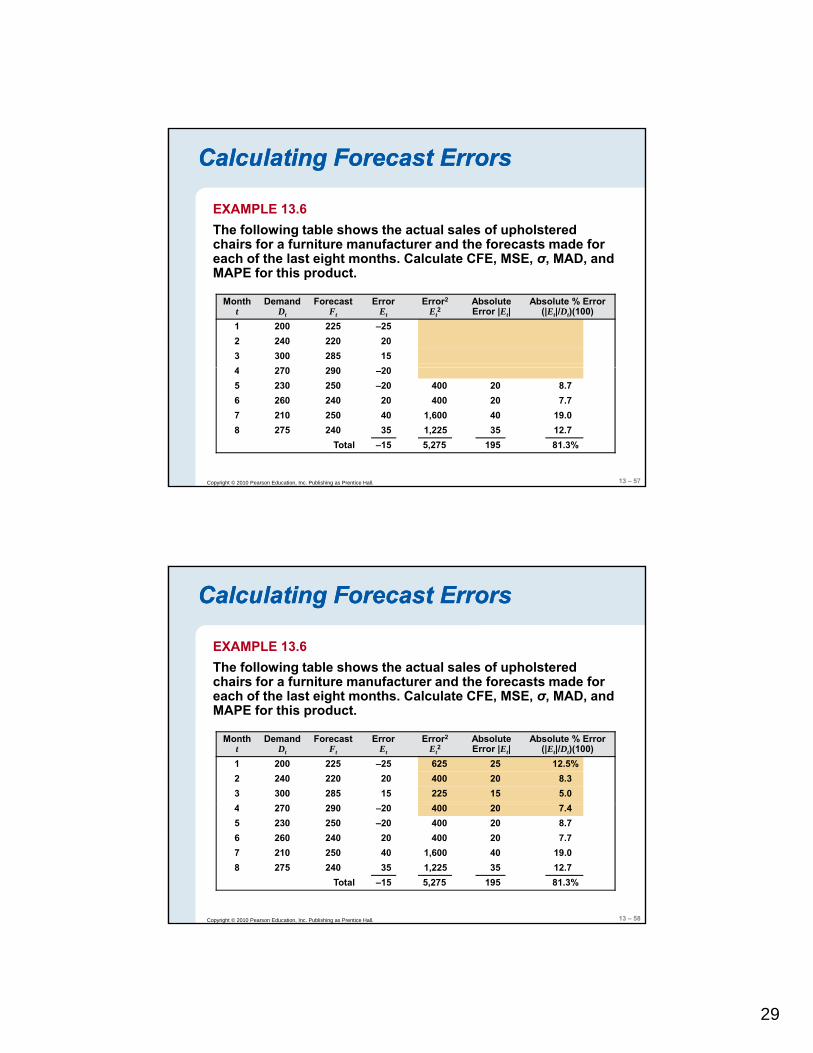
EXAMPLE 13.6The following table shows the actual sales of upholstered chairs for a furniture manufacturer and the forecasts made forchairs for a furniture manufacturer and the forecasts made for each of the last eight months. Calculate CFE, MSE, σ, MAD, and MAPE for this product.
Montht
DemandDt
ForecastFt
ErrorEt
Error2
Et2
Absolute Error |Et|
Absolute % Error (|Et|/Dt)(100)
1 200 225 –25 625 25 12.5%2 240 220 20 400 20 8.33 300 285 15 225 15 5.04 270 290 20 400 20 7 4
13 – 58Copyright © 2010 Pearson Education, Inc. Publishing as Prentice Hall.
4 270 290 –20 400 20 7.45 230 250 –20 400 20 8.76 260 240 20 400 20 7.77 210 250 40 1,600 40 19.08 275 240 35 1,225 35 12.7
Total –15 5,275 195 81.3%
30
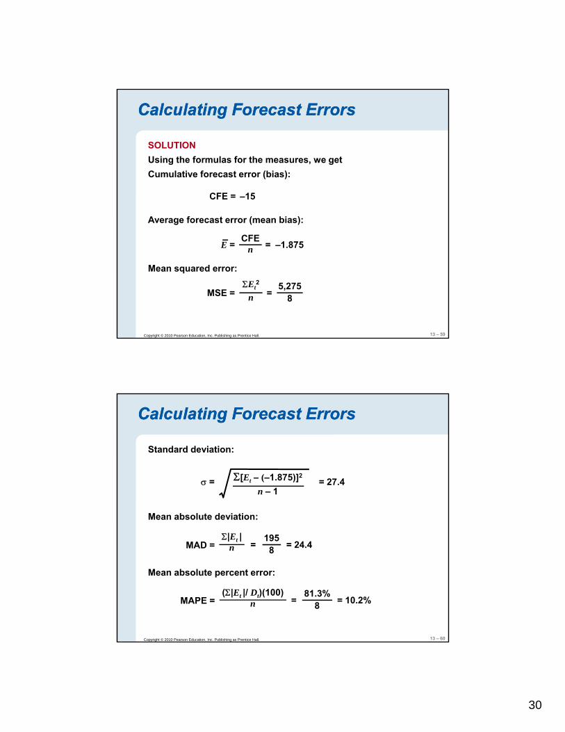
SOLUTIONUsing the formulas for the measures, we getC l ti f t (bi )
Calculating Forecast ErrorsCalculating Forecast Errors
Cumulative forecast error (bias):
CFE = –15
Average forecast error (mean bias):
CFEnE = –1.875=
13 – 59Copyright © 2010 Pearson Education, Inc. Publishing as Prentice Hall.
Mean squared error:
MSE =ΣEt
2
n5,275
8=
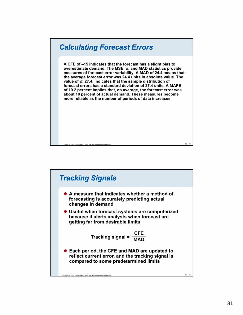
Standard deviation:
Calculating Forecast ErrorsCalculating Forecast Errors
Σ[E ( 1 875)]2
Mean absolute deviation:
Σ[Et – (–1.875)]2
n – 1σ =
Σ|Et |nMAD =
= 27.4
= = 24.41958
13 – 60Copyright © 2010 Pearson Education, Inc. Publishing as Prentice Hall.
Mean absolute percent error:
(Σ|Et |/ Dt)(100)nMAPE = = = 10.2%
81.3%8
31
Calculating Forecast ErrorsCalculating Forecast Errors
A CFE of –15 indicates that the forecast has a slight bias to overestimate demand. The MSE, σ, and MAD statistics provide measures of forecast error variability. A MAD of 24.4 means that easu es o o ecast e o a ab ty o ea s t atthe average forecast error was 24.4 units in absolute value. The value of σ, 27.4, indicates that the sample distribution of forecast errors has a standard deviation of 27.4 units. A MAPE of 10.2 percent implies that, on average, the forecast error was about 10 percent of actual demand. These measures become more reliable as the number of periods of data increases.
13 – 61Copyright © 2010 Pearson Education, Inc. Publishing as Prentice Hall.
Tracking SignalsTracking Signals
A measure that indicates whether a method of forecasting is accurately predicting actual changes in demandchanges in demandUseful when forecast systems are computerized because it alerts analysts when forecast are getting far from desirable limits
Tracking signal =CFEMAD
13 – 62Copyright © 2010 Pearson Education, Inc. Publishing as Prentice Hall.
MAD
Each period, the CFE and MAD are updated to reflect current error, and the tracking signal is compared to some predetermined limits
32
Tracking SignalsTracking Signals
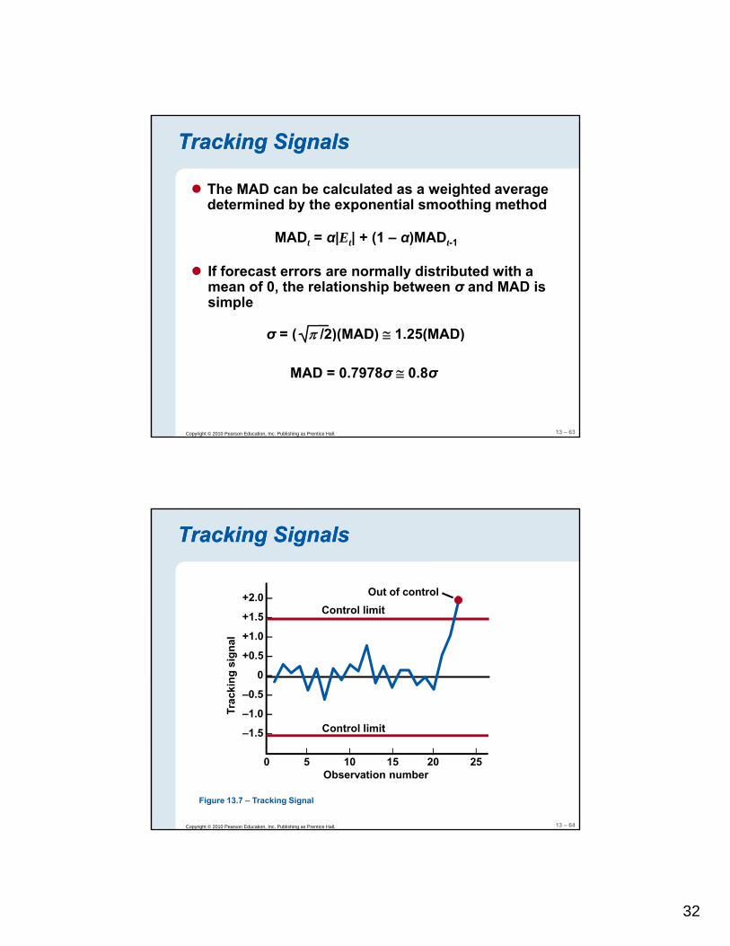
The MAD can be calculated as a weighted average determined by the exponential smoothing method
MADt = α|Et| + (1 – α)MADt-1
If forecast errors are normally distributed with a mean of 0, the relationship between σ and MAD is simple
( /2)(MAD) 1 25(MAD)
13 – 63Copyright © 2010 Pearson Education, Inc. Publishing as Prentice Hall.
σ = ( π /2)(MAD) ≅ 1.25(MAD)
MAD = 0.7978σ ≅ 0.8σ
+2.0 –
+1 5
Out of control
Tracking SignalsTracking Signals
Control limit+1.5 –
+1.0 –
+0.5 –
0 –
–0.5 –
–1.0 –Trac
king
sig
nal
13 – 64Copyright © 2010 Pearson Education, Inc. Publishing as Prentice Hall.
–1.5 –| | | | |
0 5 10 15 20 25Observation number
Control limit
Figure 13.7 – Tracking Signal
33
Criteria for Selecting MethodsCriteria for Selecting Methods
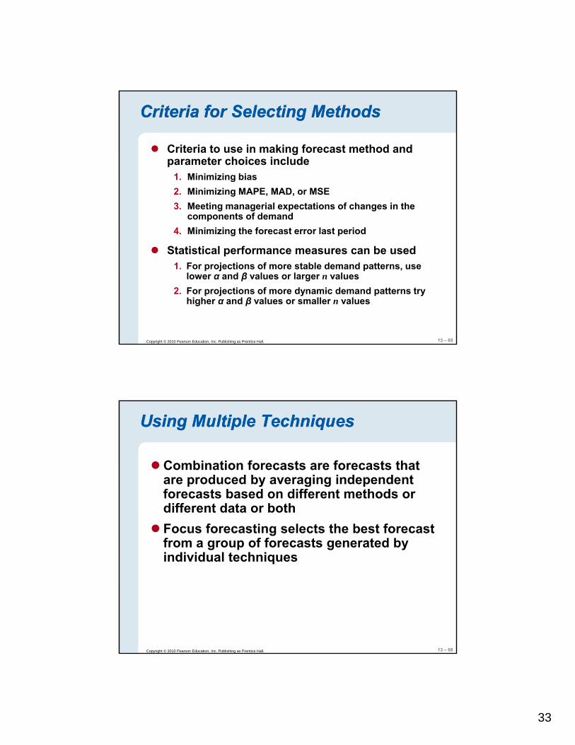
Criteria to use in making forecast method and parameter choices include
1 Minimizing bias1. Minimizing bias2. Minimizing MAPE, MAD, or MSE3. Meeting managerial expectations of changes in the
components of demand4. Minimizing the forecast error last period
Statistical performance measures can be used
13 – 65Copyright © 2010 Pearson Education, Inc. Publishing as Prentice Hall.
1. For projections of more stable demand patterns, use lower α and β values or larger n values
2. For projections of more dynamic demand patterns try higher α and β values or smaller n values
Using Multiple TechniquesUsing Multiple Techniques
Combination forecasts are forecasts that are produced by averaging independent p y g g pforecasts based on different methods or different data or bothFocus forecasting selects the best forecast from a group of forecasts generated by individual techniques
13 – 66Copyright © 2010 Pearson Education, Inc. Publishing as Prentice Hall.
34
Forecasting as a ProcessForecasting as a Process
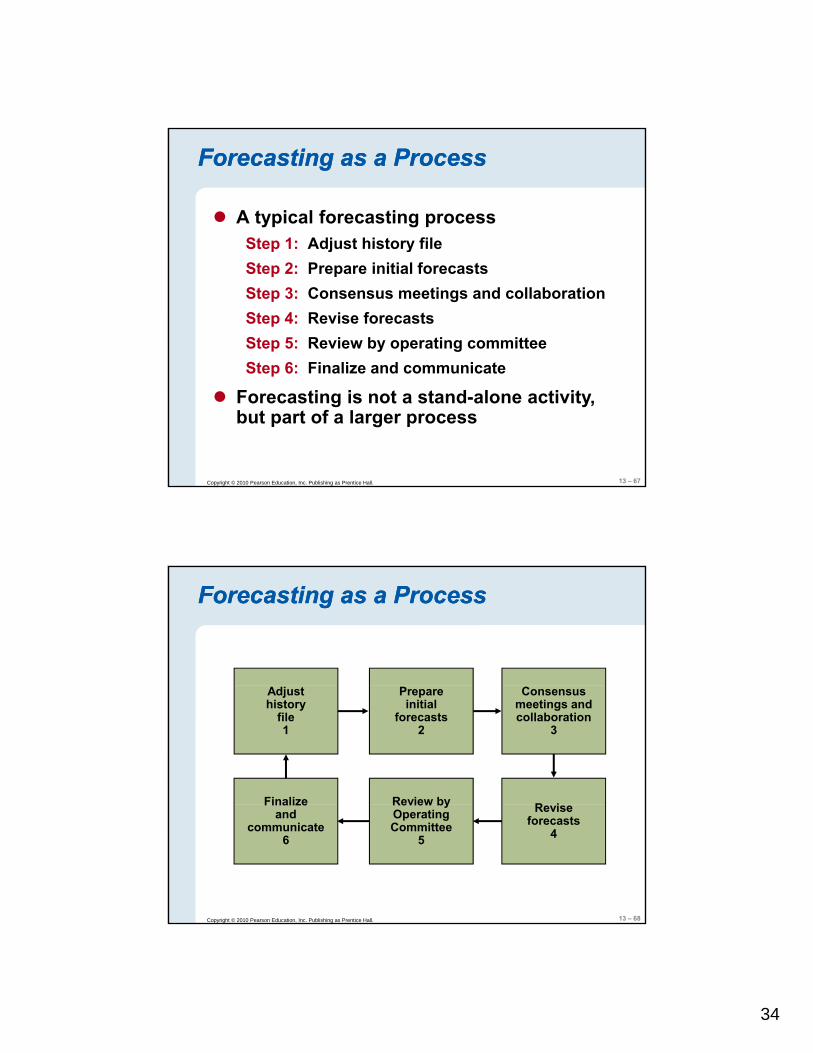
A typical forecasting processStep 1: Adjust history fileStep 1: Adjust history fileStep 2: Prepare initial forecastsStep 3: Consensus meetings and collaborationStep 4: Revise forecastsStep 5: Review by operating committeeStep 6: Finalize and communicate
13 – 67Copyright © 2010 Pearson Education, Inc. Publishing as Prentice Hall.
Step 6: Finalize and communicate
Forecasting is not a stand-alone activity, but part of a larger process
Forecasting as a ProcessForecasting as a Process
Finalize Review by R i
Consensus meetings and collaboration
3
Prepare initial
forecasts2
Adjust history
file1
13 – 68Copyright © 2010 Pearson Education, Inc. Publishing as Prentice Hall.
Finalize and
communicate6
Review by Operating Committee
5
Revise forecasts
4
35
Forecasting PrinciplesForecasting Principles
TABLE 13.2 | SOME PRINCIPLES FOR THE FORECASTING PROCESS
Better processes yield better forecasts
Demand forecasting is being done in virtually every company, either formally or informally. The challenge is to do it well—better than the competitionBetter forecasts result in better customer service and lower costs, as well as better relationships with suppliers and customersThe forecast can and must make sense based on the big picture, economic outlook, market share, and so onThe best way to improve forecast accuracy is to focus on reducing forecast error
Bi i th t ki d f f t t i f bi
13 – 69Copyright © 2010 Pearson Education, Inc. Publishing as Prentice Hall.
Bias is the worst kind of forecast error; strive for zero bias
Whenever possible, forecast at more aggregate levels. Forecast in detail only where necessaryFar more can be gained by people collaborating and communicating well than by using the most advanced forecasting technique or model
Solved Problem 1Solved Problem 1
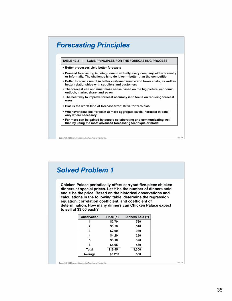
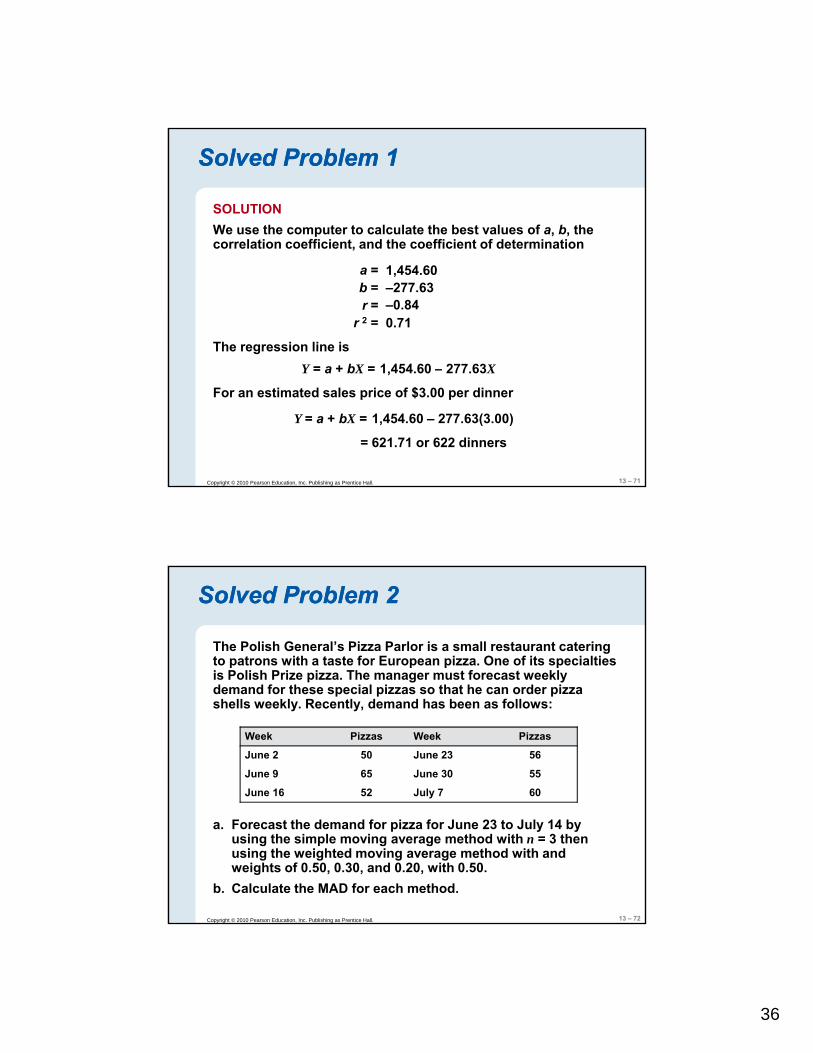
Chicken Palace periodically offers carryout five-piece chicken dinners at special prices. Let Y be the number of dinners sold and X be the price. Based on the historical observations and
l l ti i th f ll i t bl d t i th icalculations in the following table, determine the regression equation, correlation coefficient, and coefficient of determination. How many dinners can Chicken Palace expect to sell at $3.00 each?
Observation Price (X) Dinners Sold (Y)1 $2.70 7602 $3.50 5103 $2 00 980
13 – 70Copyright © 2010 Pearson Education, Inc. Publishing as Prentice Hall.
3 $2.00 9804 $4.20 2505 $3.10 3206 $4.05 480
Total $19.55 3,300Average $3.258 550
36
Solved Problem 1Solved Problem 1
SOLUTIONWe use the computer to calculate the best values of a, b, the correlation coefficient, and the coefficient of determinationcorrelation coefficient, and the coefficient of determination
a =b =r =
r 2 = 0.71–0.84–277.631,454.60
The regression line isY = a + bX = 1 454 60 277 63X
13 – 71Copyright © 2010 Pearson Education, Inc. Publishing as Prentice Hall.
Y = a + bX = 1,454.60 – 277.63X
For an estimated sales price of $3.00 per dinner
Y = a + bX = 1,454.60 – 277.63(3.00)
= 621.71 or 622 dinners
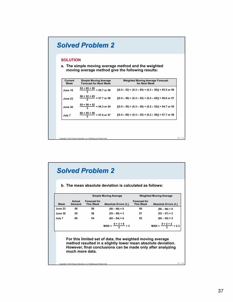
Solved Problem 2Solved Problem 2
The Polish General’s Pizza Parlor is a small restaurant catering to patrons with a taste for European pizza. One of its specialties is Polish Prize pizza. The manager must forecast weekly d d f th i l i th t h d idemand for these special pizzas so that he can order pizza shells weekly. Recently, demand has been as follows:
Week Pizzas Week Pizzas
June 2 50 June 23 56
June 9 65 June 30 55
June 16 52 July 7 60
13 – 72Copyright © 2010 Pearson Education, Inc. Publishing as Prentice Hall.
a. Forecast the demand for pizza for June 23 to July 14 by using the simple moving average method with n = 3 then using the weighted moving average method with and weights of 0.50, 0.30, and 0.20, with 0.50.
b. Calculate the MAD for each method.
37
Solved Problem 2Solved Problem 2
SOLUTIONa. The simple moving average method and the weighted
moving average method give the following results:moving average method give the following results:
Current Week
Simple Moving Average Forecast for Next Week
Weighted Moving Average Forecast for Next Week
June 16
June 23
= 55.7 or 5652 + 65 + 50
3[(0.5 × 52) + (0.3 × 65) + (0.2 × 50)] = 55.5 or 56
= 57.7 or 5856 + 52 + 65
3
55 + 56 + 52
[(0.5 × 56) + (0.3 × 52) + (0.2 × 65)] = 56.6 or 57
13 – 73Copyright © 2010 Pearson Education, Inc. Publishing as Prentice Hall.
June 30
July 7
= 54.3 or 5455 56 52
3 [(0.5 × 55) + (0.3 × 56) + (0.2 × 52)] = 54.7 or 55
= 57.0 or 5760 + 55 + 56
3 [(0.5 × 60) + (0.3 × 55) + (0.2 × 56)] = 57.7 or 58
Solved Problem 2Solved Problem 2
b. The mean absolute deviation is calculated as follows:
Simple Moving Average Weighted Moving AverageSimple Moving Average Weighted Moving Average
WeekActual
DemandForecast for This Week Absolute Errors |Et|
Forecast for This Week Absolute Errors |Et|
June 23 56 56 56
June 30 55 58 57
July 7 60 54 55
|56 – 56| = 0
|55 – 58| = 3
|60 – 54| = 6
MAD = = 30 + 3 + 6
3 MAD = = 2.30 + 2 + 2
3
|56 – 56| = 0|55 – 57| = 2
|60 – 55| = 5
13 – 74Copyright © 2010 Pearson Education, Inc. Publishing as Prentice Hall.
For this limited set of data, the weighted moving average method resulted in a slightly lower mean absolute deviation. However, final conclusions can be made only after analyzing much more data.
38
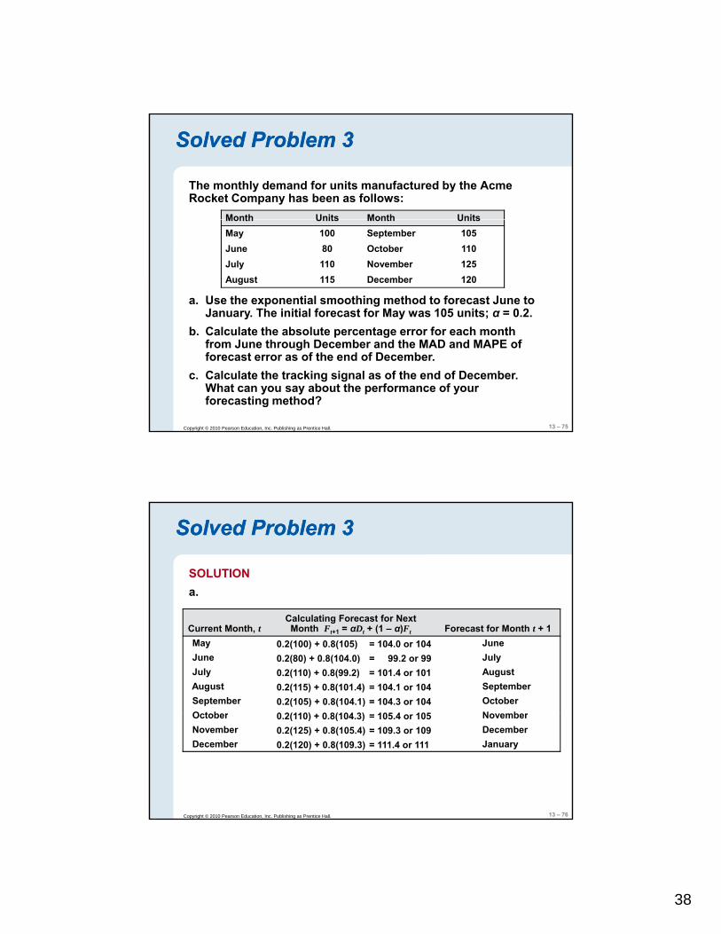
Solved Problem 3Solved Problem 3
The monthly demand for units manufactured by the Acme Rocket Company has been as follows:
Month Units Month UnitsMonth Units Month UnitsMay 100 September 105June 80 October 110July 110 November 125August 115 December 120
a. Use the exponential smoothing method to forecast June to January. The initial forecast for May was 105 units; α = 0.2.
13 – 75Copyright © 2010 Pearson Education, Inc. Publishing as Prentice Hall.
b. Calculate the absolute percentage error for each month from June through December and the MAD and MAPE of forecast error as of the end of December.
c. Calculate the tracking signal as of the end of December. What can you say about the performance of your forecasting method?
Solved Problem 3Solved Problem 3
SOLUTIONa.
Current Month, tCalculating Forecast for Next Month Ft+1 = αDt + (1 – α)Ft Forecast for Month t + 1
May JuneJune JulyJuly AugustAugust SeptemberSeptember OctoberOctober November
0.2(100) + 0.8(105) = 104.0 or 1040.2(80) + 0.8(104.0)0.2(110) + 0.8(99.2)
= 99.2 or 99= 101.4 or 101
0.2(115) + 0.8(101.4)0.2(105) + 0.8(104.1)0 2(110) + 0 8(104 3)
= 104.1 or 104= 104.3 or 104
105 4 105
13 – 76Copyright © 2010 Pearson Education, Inc. Publishing as Prentice Hall.
October NovemberNovember DecemberDecember January
0.2(110) + 0.8(104.3)0.2(125) + 0.8(105.4)0.2(120) + 0.8(109.3)
= 105.4 or 105= 109.3 or 109= 111.4 or 111
39
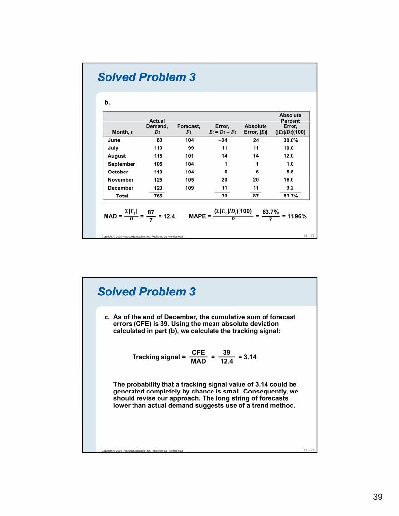
Solved Problem 3Solved Problem 3
b.
ActualAbsolute Percent
–24 24 30.0%11 11 10.0
Month, t
Actual Demand,
DtForecast,
FtError,
Et = Dt – FtAbsolute Error, |Et|
Percent Error,
(|Et|/Dt)(100)June 80 104July 110 99August 115 101September 105 104October 110 104November 125 105
14 14 12.01 1 1.06 6 5.5
20 20 16 0
13 – 77Copyright © 2010 Pearson Education, Inc. Publishing as Prentice Hall.
November 125 105December 120 109
Total 765
20 20 16.011 11 9.239 87 83.7%
Σ|Et |nMAD =
(Σ|Et |/Dt)(100)nMAPE = = = 11.96%
83.7%7= = 12.487
7
Solved Problem 3Solved Problem 3
c. As of the end of December, the cumulative sum of forecast errors (CFE) is 39. Using the mean absolute deviation calculated in part (b), we calculate the tracking signal:
The probability that a tracking signal value of 3.14 could be generated completely by chance is small. Consequently, we
Tracking signal = CFEMAD = = 3.1439
12.4
13 – 78Copyright © 2010 Pearson Education, Inc. Publishing as Prentice Hall.
g p y y q y,should revise our approach. The long string of forecasts lower than actual demand suggests use of a trend method.
40
Solved Problem 4Solved Problem 4
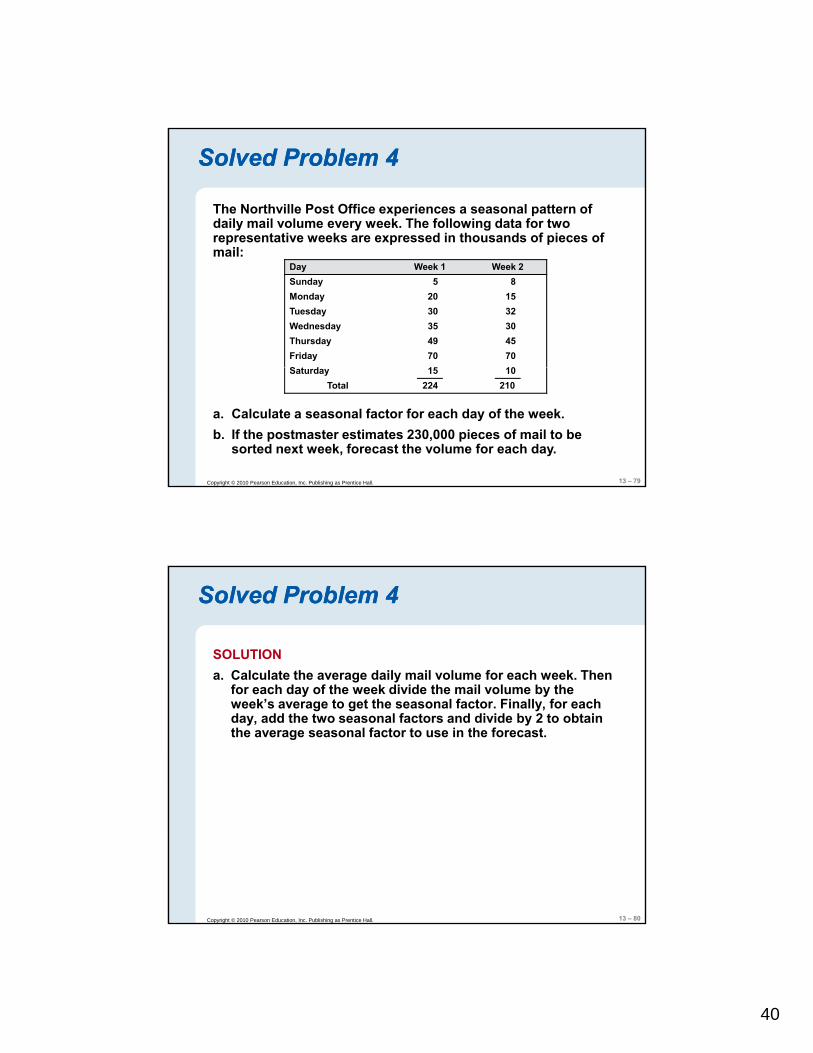
The Northville Post Office experiences a seasonal pattern of daily mail volume every week. The following data for two representative weeks are expressed in thousands of pieces of
ilmail:Day Week 1 Week 2Sunday 5 8Monday 20 15Tuesday 30 32Wednesday 35 30Thursday 49 45Friday 70 70S t d 15 10
13 – 79Copyright © 2010 Pearson Education, Inc. Publishing as Prentice Hall.
Saturday 15 10Total 224 210
a. Calculate a seasonal factor for each day of the week.b. If the postmaster estimates 230,000 pieces of mail to be
sorted next week, forecast the volume for each day.
Solved Problem 4Solved Problem 4
SOLUTIONa. Calculate the average daily mail volume for each week. Then
f h d f th k di id th il l b thfor each day of the week divide the mail volume by the week’s average to get the seasonal factor. Finally, for each day, add the two seasonal factors and divide by 2 to obtain the average seasonal factor to use in the forecast.
13 – 80Copyright © 2010 Pearson Education, Inc. Publishing as Prentice Hall.
41
Solved Problem 4Solved Problem 4
Week 1 Week 2
Mail Seasonal Factor Mail Seasonal FactorAverage
Seasonal FactorDay
Mail Volume
Seasonal Factor (1)
Mail Volume
Seasonal Factor (2)
Seasonal Factor[(1) + (2)]/2
Sunday 5 8Monday 20 15Tuesday 30 32Wednesday 35 30Thursday 49 45Friday 70 70Saturday 15 10
5/32 = 0.1562520/32 = 0.6250030/32 = 0.93750
8/30 = 0.2666715/30 = 0.5000032/30 = 1.06667
0.211460.562501.00209
35/32 = 1.0937549/32 = 1.5312570/32 = 2.1875015/32 = 0.46875
30/30 = 1.0000045/30 = 1.5000070/30 = 2.3333310/30 = 0.33333
1.046881.515632.260420.40104
13 – 81Copyright © 2010 Pearson Education, Inc. Publishing as Prentice Hall.
Total 224 210Average 224/7 = 32 210/7 = 30
Solved Problem 4Solved Problem 4
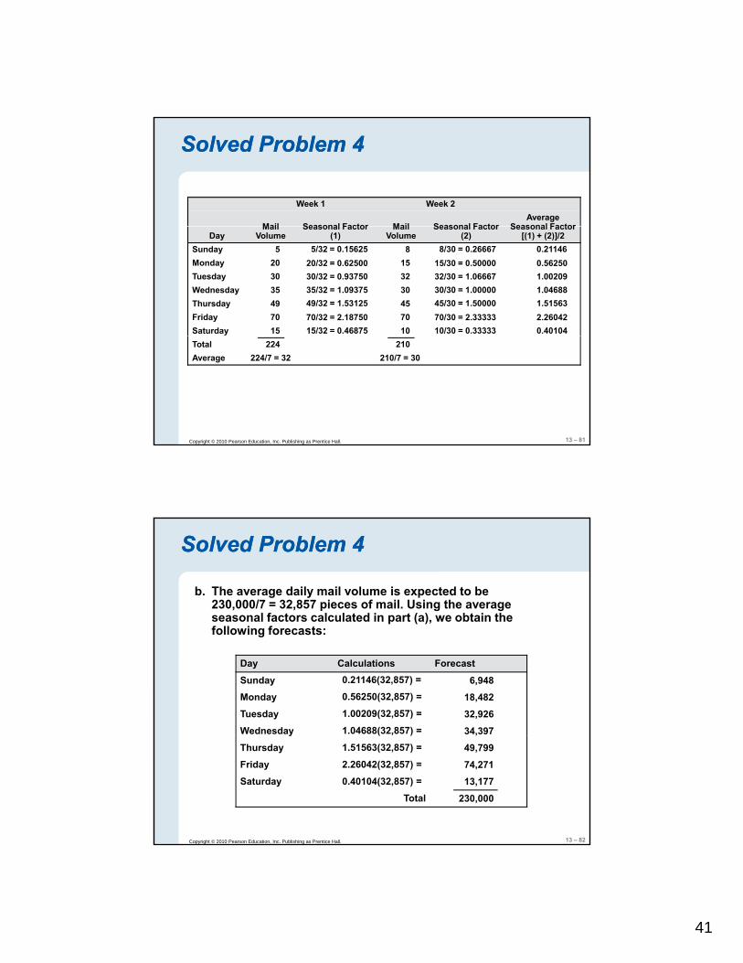
b. The average daily mail volume is expected to be 230,000/7 = 32,857 pieces of mail. Using the average seasonal factors calculated in part (a), we obtain the f ll i f tfollowing forecasts:
6,94818,482
32,926
0.21146(32,857) =
0.56250(32,857) =
1.00209(32,857) =
34,3971.04688(32,857) =
Day Calculations Forecast
SundayMonday
Tuesday
Wednesday
13 – 82Copyright © 2010 Pearson Education, Inc. Publishing as Prentice Hall.
49,799
74,271
13,177
230,000
1.51563(32,857) =
2.26042(32,857) =
0.40104(32,857) =
y
ThursdayFriday
Saturday
Total

42
13 – 83Copyright © 2010 Pearson Education, Inc. Publishing as Prentice Hall.

![krajewski om9 ppt 13.ppt - kaizenha.comkaizenha.com/cdn/files/PPC/Slides/2.pdf · Title: Microsoft PowerPoint - krajewski_om9_ppt_13.ppt [Compatibility Mode] Author: Administrator](https://img.pdfslide.us/doc/110x75/5b7978787f8b9ad77e8d9974/krajewski-om9-ppt-13ppt-title-microsoft-powerpoint-krajewskiom9ppt13ppt.jpg)


![Krajewski Om9 Ppt 14 [Compatibility Mode]](https://img.pdfslide.us/doc/110x75/55cf9b82550346d033a659f8/krajewski-om9-ppt-14-compatibility-mode.jpg)