Embed Size (px)
Citation preview

20
A E S T I T I OM A
RESE
ARCH ARTICLE aestimatio, the ieb international journal of finance, 2013. 6: 20-49
© 2013 aestimatio, the ieb international journal of finance
firms’ accrualsand Tobin’s qCalmès, Christian; Cormier, Denis; Racicot, François-Éric and Théoret, Raymond
� RECEIVED : 12 DECEMBER 2012� ACCEPTED : 8 FEBRUARY 2013
Abstract
According to the neoclassical theory of investment, if firms’ accruals are a form of
short-term investment they should be greatly influenced by the shadow price of
capital, namely Tobin’s q. In the presence of financial market imperfections, cash-flows should also impact accruals since they proxy for liquidity constraints. In this
paper, we test a new version of the cash-flows augmented accrual model featuring a
proxy for Tobin’s q, and compare it to the most common models found in theliterature. To deal with the measurement errors often encountered in accounting data
and Tobin’s q empirical proxies, we rely on a modified version of the Hausmanartificial regression, and find that all the key parameters of the accrual models are
indeed systematically biased with measurement errors. More importantly, our findings
largely qualify the accrual investment perspective, as both cash-flows and Tobin’s qare found strongly significant regressors of firms’ accruals. Interestingly, we find that
the Tobin’s q augmented model is able to isolate discretionary accruals, and to deliverresiduals quite close to zero on average.
Keywords:
Discretionary accruals, Investment, Tobin’s q, Cash-flows, Measurement errors, Instrumental variable estimators.
JEL classification:
M41, C12, D92.
Calmès, C. Université du Québec (Outaouais), 101 St. Jean Bosco, Gatineau, Québec, Canada, J8X 3X7. Chaire d’information financière et organisationnelle, École des sciences de la gestion (UQAM). Laboratory for Research in Statistics and Probability (Carleton University).E-mail: [email protected]
Cormier, D. Chaire d’information financière et organisationnelle, École des sciences de la gestion (UQAM). Université du Québec (Mon-tréal), 315 Ste. Catherine est, Montréal, Québec, Canada, H2X 3X2. E-mail: [email protected]
Racicot, F.E. Telfer School of Management, Member of the CGA-Canada Accounting and Governance Research Centre (CGA-AGRC),Universityof Ottawa, Canada. Chaire d’information financière et organisationnelle, ESG-UQAM. Address: 55 Laurier Avenue East, Ottawa Ontario,K1N 6N5, Canada. 613-562-5800 (4757). E-mail: [email protected]
Théoret, R. Université du Québec (Montréal), 315 Ste. Catherine est, Montréal, Québec, Canada, H2X 3X2. Professeur associé (UQO).Chaire d’information financière et organisationnelle, École des sciences de la gestion (UQAM). E-mail: [email protected]
+1 514 987 3000 4417.

21
A E S T I T I OM A
21
aestimatio, the ieb international journal of finance, 2013. 6: 20-49
© 2013 aestimatio, the ieb international journal of finance
los ajustes por devengo delas empresas y la q de TobinCalmès, Christian; Cormier, Denis; Racicot, François-Éric and Théoret, Raymond
Resumen
De acuerdo con la teoría neoclásica de la inversión, si los ajustes por devengo de las em-
presas constituyen una forma de inversión a corto plazo, deberían estar fuertemente in-
fluenciados por el precio sombra del capital, denominado q de Tobin. En presencia deimperfecciones de mercado, los flujos de caja también deberían influenciar los ajustes
por devengo ya que son una variable proxy de las restricciones de liquidez. En este artículo
se contrasta una nueva versión del modelo de ajustes por devengo aumentado con flujos
de caja con una variable proxy para la q de Tobin, el cual se compara con los modelosque habitualmente se pueden encontrar en la literatura. Para tratar la cuestión de los
errores de medida que a menudo se encuentran cuando se trabaja con datos contables y
variables proxy empíricas de la q de Tobin, nos apoyamos en una versión modificada dela regresión artificial de Haussman, encontrando que todos los parámetros clave de los
modelos de ajuste por devengo están sistemáticamente sesgados debido a los errores de
medida. Más importante aún es el hecho de que nuestros resultados sostienen en gran
medida la perspectiva de los intereses devengados, ya que tanto los flujos de caja como
la q de Tobin son regresores altamente significativos de los ajustes por devengo de las em-presas. También resulta interesante el hecho de que el modelo aumentado de la q deTobin es capaz de aislar los ajustes por devengo discrecionales, y que los residuos de la
ecuación se adaptan muy bien a la predicción de los rendimientos de las acciones.
Palabras clave:
Ajustes por devengo discreccionales, inversión, q de Tobin, flujos de caja, errores de me-dida, estimadores de variables instrumentales.

22
A E S T I T I OM A
firm
s’ a
ccru
als
and
tobi
n’s
q. Ca
lmès
, C., C
orm
ier,
D., R
acico
t, F.E
. and
Thé
oret
, R.
aes
tim
at
io, t
he
ieb
int
ern
at
ion
al
jou
rn
al
of
fin
an
ce,
2013
. 6: 2
0-49
n 1. Introduction
A fundamental drawback of cash-flows is that they present timing and matching
problems that cause them to be a very noisy measure of firm performance. To mitigate
these issues, it is common to rely on accounting accruals to intertemporally smooth
earnings. Accruals are then used to separate the timing of cash flows from their
accounting recognition. Based on the cash-flows statement, total accruals, the sum of
discretionary and non-discretionary accruals, are defined as the difference between firm
earnings and cash-flows (Jones, 1991; Bartov et al., 2001), and, as such, are related to
firm performance. For this reason, accrual models are widely used by financial analysts
to assess the level of discretionary accruals, a significant predictor of stocks returns1
(Sloan, 1996; Dechow and Dichev, 2002; Fama and French, 2007; Hirshleifer et al.,
2009). Actually, one of the main reasons why accrual models have generated such
attention in the finance literature is precisely the fact that the accrual equations residuals
carry valuable information about stock returns. This relates to the famous accrual
anomaly (Sloan, 1996; Dechow and Dichev, 2002), which, contrary to the asset growth
and profitability anomalies, seems to be very robust (Fama and French, 2007). To better
isolate the nonlinear relationship between accruals and firm performance, researchers
often include proxies for economic values and investment potential such as property
plant and equipment (PPE) and sales. However, the literature is almost mute about theinvestment perspective of accruals, even though accruals measure investment in working
capital. According to this perspective, the standard specification of the accrual models
misses some important aspects of accruals, namely the fact that accruals constitute a
form of short-term investment, at least in terms of working capital. In particular, the
accrual anomaly might actually relate to the investment information embedded in
accruals. For example, Wu et al. (2007, 2010) show that the negative relationship
between accruals and the discount rate helps explain the accruals anomaly.
In this paper, our motivation is to build an accrual model consistent with the neoclassical
theory of investment to study the positive relationship between accruals and investment
variables. In the literature, the standard models used to estimate non-discretionary
accruals generally rely on OLS estimation (e.g., Jones, 1991; Bartov et al., 2001; Xie,
2001, Kothari et al., 2005; Wu et al., 2007, 2010 among many others). It is also common
to use models taking into account various aspects of simultaneity biases and address
the problem of measurement errors associated with accruals (e.g. Kang and
Sivaramakrishnan, 1995; Hansen, 1999; Young, 1999; Hribar and Collins, 2002; Zhang,
2007; Ibrahim, 2009). To control for firm performance, many studies include a variable
such as ROA, since accruals and performance are positively related (e.g., Kothari et al.2005). By contrast, in this paper, we focus on two commonly used accrual models, the
1 For an extensive survey on the relationship between accounting information and capital markets efficiency see Kothari (2001).

23
A E S T I T I OM A
firms’ a
ccruals and tobin’s q. Calm
ès, C., Cormier, D
., Racicot, F.E. and Théoret, R.a
estim
at
io, t
he
iebin
ter
na
tio
na
ljo
ur
na
lo
ffin
an
ce, 2013. 6
: 20-49
Jones (1991) model, our benchmark, and the cash-flows augmented Jones model
(Dechow, 1994; Dechow and Dichev, 2002; Hirshleifer et al., 2004; Zhang, 2007;
Hirshleifer et al., 2009) to compare them with a new type of model where firms’ accruals
are explicitly specified as short-term investment. According to the neoclassical theory,
Tobin’s q (the shadow price of capital) is a key explanatory variable of investment (e.g.Abel and Blanchard, 1983; Fazzari et al., 1988; Blanchard and Fischer, 1989; Gilchrist
and Himmelberg, 1995; or Brown and Petersen, 2009 and Brown et al., 2009). In this
sense, if accruals are indeed a form of short-term investment, they should be influenced
by Tobin’s q. Relatedly, our approach aims at rigorously justifying the introduction ofcash-flows in the accrual models, investment theory predicting that cash-flows proxy
for firms’ liquidity constraints. The main contribution of this paper is thus to propose a
model where accruals are a function of investment variables.
Relatedly, the inclusion of Tobin’s q adds to the endogeneity problem often
encountered in accrual models, since this variable is notoriously plagued with
measurement errors, a well documented fact in the investment literature (e.g.,
Hayashi, 1982; Erickson and Withed, 2000, 2002, among many others). Furthermore,
when examining non-discretionary and discretionary accruals — the latter being the
error term in the accrual models — we have to bear in mind the fact that this error
term is the portion of accruals managed by firms, so that it may sometimes be
influenced by various earnings management practices (Dechow et al., 1995;
Burghstahler and Dichev, 1997; DeFond and Park, 1997; DeGeorge, Patel and
Zeckhauser, 1999; Peasnell et al., 2000; Xie, 2001; Leuz, Nanda and Wysocky, 2003;
Marquardt and Wiedman, 2004; Hirshleifer et al., 2004; Roychowdhury, 2006). This
may result in a statistical anomaly worth detecting, as discretionary accruals are often
used to forecast market returns. The accrual models sometimes account for
heteroskedasticity with a form of weighted least-squares, but the measurement errors
inherent to accounting data are usually assumed to be systematically biased in the
same direction, even though they can cause a serious bias in the estimation if the
orthogonality between the explanatory variables and the equation innovation is not
satisfied. Rigorously correcting for measurement errors is thus imperative, and it is
much desirable to resort to a robust estimation method in order to compute the
accruals with the greatest possible accuracy (Ibrahim, 2009). To handle this task, we
introduce new instruments based on a weighted optimal matrix of the higher
moments of the explanatory variables, and apply these optimal instruments to an
Hausman artificial regression (our Haus-C method).
Our results suggest that measurement errors have indeed a great influence on the
parameters estimation of the basic Jones model. More precisely, our estimation of
the accrual models confirms that important measurements errors contaminate the
accounting measures of changes in sales and fixed assets, the two main explanatory

variables of the Jones model. More importantly, our main finding suggests that,
Tobin’s q, which has already a very significant positive impact on non-discretionaryaccruals when using the standard OLS method, displays an increased explanatory
power when applying our Haus-C procedure. The Haus-C procedure delivers a
coefficient of the error adjustment regressor comparable, in level, to the Tobin’s qcoefficient itself. We can interpret this result as new evidence that firms’ expectations
are partly incorporated in future cash-flows, a point often mentioned in the empirical
literature on investment. Relatedly, when we introduce Tobin’s q in the accrualsequation, the cash-flow variable has a smaller influence on short-term investment.
When measurement errors are properly accounted for, the role of Tobin’s q isreinforced, while cash-flows seem to play a minor role, although non-trivial. Overall,
the evidence we gather tends to support the empirical literature on firm investment,
and in particular the idea that market imperfections also impend the Modigliani and
Miller theorem to hold for short-term investment. In the context of accruals, these
imperfections are likely associated with the liquidity constraints in earnings
management and the preference for directly self-financing accruals with cash-flows
before resorting to external finance.
This paper is organized as follows. In section 2 we present the theoretical underpinning
of our approach, based on the neoclassical theory of investment, and describe the
three accrual models we analyze, along with some considerations regarding
measurement errors. In section 3 we detail the empirical results, and in section 4 we
compare the residuals of our accrual equations to assess the performance of the
Tobin’s q augmented model. Section 5 concludes.
n 2. The Model
With a balance sheet approach, total accruals are defined as:
TA≡ (ΔCA–ΔCASH)–(ΔCL–ΔSTD–ΔTP )–DEP (1)
where ΔCA stands for change in current assets; ΔCASH, change in cash or cashequivalents; ΔCL, change in current liabilities; ΔSTD, change in debt included in currentliabilities; ΔTP, change in income taxes payable; and DEP represents the depreciationand amortization expenses. Note however that the negative depreciation term in the
traditional accruals equation tends to strongly influence the model’s fit, as the
depreciation to assets ratio is five times higher than the accounts receivable and accounts
payable, on average (Barth, Cram and Nelson, 2001). One way to deal with this issue
is to look at short-term accruals and omit the long-run component, i.e., the depreciation
(Teoh et al., 1998a, b). Since this study focuses on the short-term investment dimension
24
A E S T I T I OM A
firm
s’ a
ccru
als
and
tobi
n’s
q. Ca
lmès
, C., C
orm
ier,
D., R
acico
t, F.E
. and
Thé
oret
, R.
aes
tim
at
io, t
he
ieb
int
ern
at
ion
al
jou
rn
al
of
fin
an
ce,
2013
. 6: 2
0-49

of firms’ accruals (the working capital component of accruals), we thus consider an
alternative construct, CA which eliminates total depreciation from Equation (1).
2.1. Theoretical underpinningTo cast accruals in terms of short-term investment we resort to the neoclassical theory
of investment, and in particular to the q theory of investment (Abel and Blanchard,1983; Blanchard and Fischer, 1989; Adda and Cooper, 2003) which predicts that only
one variable impacts investment, I, namely the shadow price of capital, Tobin’s q, avariable incorporating all the relevant information related to the investment decision.
In theory, investment is expressed as:
= j(qit) (2)
Where the i subscript refers to an individual firm or plant, and the t subscript representstime, whereas kit is the firm’s capital stock. This equation is the result of an
intertemporal optimization program based on the maximization of the utility of a
representative consumer subject to a resource constraint (Abel and Blanchard, 1983).
In Equation (2), q accounts for both the gross return and the cost of capital, and issimply defined as the market value of capital over its replacement cost (Tobin, 1969).
More precisely, in a general equilibrium setting à la Ramsey, this variable is the shadow
price of capital, which is equal to the present discounted value of capital future
marginal products. At the margin, the central planner who computes the optimization
program equates the value of an additional unit of capital with its marginal cost,
which increases with the rate of investment. The main implication of the theory is
then: j ’(qit)>0 .
To test it, Equation (2) is usually linearized as follows:
= a0+a1qit (3)
the coefficient a1 being related to the agent discount rate and to the adjustment costs
of capital. Generally, researchers scale investment by assets instead of capital, which
in our case is also more in line with the accruals accounting framework. Equation (3)
is derived under the assumption of perfect markets. However, if markets are imperfect,
financial imperfections and the liquidity constraints they entail may impact investment.
In the context of market imperfections and credit market frictions, it is thus common
to augment Equation (3) with a vector Xt of control variables2:
= a0+a1qit+Xtθ (4)
25
A E S T I T I OM A
firms’ a
ccruals and tobin’s q. Calm
ès, C., Cormier, D
., Racicot, F.E. and Théoret, R.a
estim
at
io, t
he
iebin
ter
na
tio
na
ljo
ur
na
lo
ffin
an
ce, 2013. 6
: 20-49
Iit
kit
Iit
Ait
Iit
Ait
2 As explained in the following section, nominal variables in the X vector are also scaled by assets.

In addition to Tobin’s q, in many studies, measures of cash flows are found significantfactors influencing investment (e.g. Gilchrist and Himmelberg, 1995; Calmès, 2004,
Brown et al., 2009; Brown and Petersen, 2009). If market imperfections are at work,
the relationship between investment and cash-flows ought to be positive since external
finance is more costly than internal finance. Measures of profits may be also added to
the control variables set to account for liquidity constraints. This generalization is still
much debated in the literature because it is obviously at odds with the Modigliani and
Miller (1958) theorems on the independence between the firm’s structure of capital
and its value, a result based on perfect financial markets. In this paper, we introduce
a new specification of firms’ accruals based on this theoretical underpinning, directly
derived from Equation (4), as discussed below.
2.2. The empirical framework
2.2.1. The Jones Model of Accruals
The Jones (1991) model, our primary benchmark (model 1), is the most popular
accrual model in the accounting literature. It does not rely on any economic or financial
theory, but is rather an empirical model which relates the components of accruals to
their statistical determinants as follows:
= as ( )+bs ( )+ds ( )+eit = +eit (5)
where TA is total accruals; A, total assets; PPE, gross property plant and equipmentat the end of year t ; and ΔREV represents revenues in year t less revenues in year (t–1).As usually done in the literature, we scale all variables by Ai,t–1 to account for the
heteroskedasticity which might be present in eit . This precaution also helps control for
size effects. Equation (5) may be decomposed in two parts, the non-discretionary
accruals component and the discretionary accruals one. The fitted value of the
equation, , represents the non-discretionary accruals, while the innovation, eit , is
the discretionary part of accruals. Two control variables of the benchmark model
relate, respectively, to the two main components of accruals, working capital and
depreciation. The first control variable, ΔREVit , often replaced by the change in sales
in the literature (e.g., Cormier et al., 2000), is associated with working capital, while
the second control variable, PPEit , is linked to depreciation. Usually, the ΔREVit
coefficient is found positively related to total accruals. Indeed, an increase in ΔREVit
should lead to an increase in working capital since accounts receivable are generally
more sensitive to changes in sales than accounts payable3. Furthermore, the coefficient
of PPEit should be negative as PPEit determines the depreciation expenses, a negative
component of accruals. Note however that there is potentially an endogeneity issue
26
A E S T I T I OM A
firm
s’ a
ccru
als
and
tobi
n’s
q. Ca
lmès
, C., C
orm
ier,
D., R
acico
t, F.E
. and
Thé
oret
, R.
aes
tim
at
io, t
he
ieb
int
ern
at
ion
al
jou
rn
al
of
fin
an
ce,
2013
. 6: 2
0-49
3 In some cases, the sign of this coefficient may be negative. For more details, see McNichols and Wilson (1988).
TAitAi,t–1
TÂitAi,t–1
1Ai,t–1
ΔREVitAi,t–1
PPEitAi,t–1
TÂitAi,t–1

here because the control variable PPEit might be collinear to accruals, the link between
depreciation and PPEit being quite strong.
In the short-term version of the model we adopt, we omit DEP on the LHS and PPEon the RHS of Equation (5). In this case, Equation (6) obtains:
= as ( )+ds ( )+eit (6)
Finally, note that, in principle, even though the Jones model is simply an accounting
specification of non-discretionary accruals, it remains perfectly compatible with our
investment setting (Equation 4), as the explanatory variables appearing in the Jones
model may be included in the vector of control variables X. However, investigating aninvestment specification, the introduction of these variables in accruals models is not
only justified by a statistical bijection between a component of accruals and its
accounting determinants, like the accounting dependence of working capital on
change in revenues. For instance, in Equation (6), with our investment framework, the
change in revenues can be interpreted as a standard liquidity constraint.
2.2.2. The Cash-flows Augmented Jones Model
To account for firm performance it is common to introduce cash-flows (CF ) in theaccrual models (e.g., Dechow, 1994; McNichols, 2002; Francis et al., 2005 and Zhang,
2007). In its long-term form, this standard accrual model (model II) can be written as:
= as ( )+bs ( )+ds ( )+ks ( )+eit (7)
The corresponding short-term version of Equation (7) we consider is then:
= as ( )+ds ( )+ks ( )+eit (8)
In our framework, the introduction of the cash-flows variable may not be viewed simply
as an ad hoc way of controlling for firm performance, but as a variable proxying for the
liquidity and financial constraints stemming from market imperfections. In other
words, our approach provides a direct, theoretically founded justification of the
influence of the cash-flows variable on firms’ accruals.
A standard procedure often found in the accounting literature is to lag cash-flows to
correct for endogeneity. This procedure is generally adequate to mitigate the error term
autocorrelation but less appropriate to tackle the endogeneity issue per se (Theil, 1953).
Hence, in our approach, we replace the cash-flows variable by its predicted (fitted)
value to ensure its orthogonality with the error term. An intuitive justification for doing
so is that accruals are often value related, particularly so for outperforming firms, that
27
A E S T I T I OM A
firms’ a
ccruals and tobin’s q. Calm
ès, C., Cormier, D
., Racicot, F.E. and Théoret, R.a
estim
at
io, t
he
iebin
ter
na
tio
na
ljo
ur
na
lo
ffin
an
ce, 2013. 6
: 20-49
CAitAi,t–1
1Ai,t–1
ΔREVitAi,t–1
TAitAi,t–1
CFitAi,t–1
1Ai,t–1
ΔREVitAi,t–1
CAitAi,t–1
CFitAi,t–1
1Ai,t–1
ΔREVitAi,t–1
PPEitAi,t–1

is firms characterized by high Tobin’s q and strong persistence in sales. Indeed, forthese firms, accruals are strongly (positively) autocorrelated and also quite correlated
with cash-flows. Relatedly, even though accrual persistence can be partly attributable
to a cosmetic smoothing through the strategic allocation of accruals over few
accounting periods, and to various earnings management practices or adjustment
costs4 (including hiding information on current sales innovation), accrual persistence
is also explained by firm performance, and, consequently, by expected cash-flows. As
a matter of fact, note that this observation directly relates to the investment perspective
on accruals. Indeed, the literature on firm investment suggests that cash flows are one
of the main driving forces of investment. Hence, if accruals can be considered as a
form of short-term investment, the cash-flows variable should be found a positive,
significant factor influencing accruals.
2.2.3. The Tobin’s q Accrual Model
Consistent with Zhang (2007) view on the investment perspective of firms’ accruals,
we propose a new accrual model, model III, for which we adapt Equation (4), and
directly introduce Tobin’s q as an explanatory variable of firms’ accruals:
= b1 ( )+b2 +b3 +b4 +b5 +xit (9)
where Tobin’s q is proxied empirically by:
Market value of capital + Accounting value of debts (10)Accounting value of assets
Note that q is theoretically defined as a marginal concept, while Equation (10) definesit as an average one5. The marginal concept is unobservable, so researchers usually
define Tobin’s q on an average basis. When q is computed this way, Equation (9)establishes a direct link between accruals and the stock market valuation of the firm.
In this sense, q directly controls for firm performance in Equation (9). Note also thatthere are many empirical proxies of Tobin’s q in the investment literature, includingvariables based on working capital. For example, one popular measure used in financial
studies proxies Tobin’s q with the ratio of the market value of assets to theirreplacement cost, as originally defined by Tobin (1969). However, since we work in
an accounting framework, we rely on an accounting definition of Tobin’s q to be moreconsistent with the literature. In this literature, Tobin’s q is usually measured as themarket-to-book ratio, i.e., the market value of equity scaled by its book value. However,
28
A E S T I T I OM A
firm
s’ a
ccru
als
and
tobi
n’s
q. Ca
lmès
, C., C
orm
ier,
D., R
acico
t, F.E
. and
Thé
oret
, R.
aes
tim
at
io, t
he
ieb
int
ern
at
ion
al
jou
rn
al
of
fin
an
ce,
2013
. 6: 2
0-49
4 Note that the neoclassical theory of investment suggests that autocorrelation will be present in the estimation of the investmentfunction because of the convex cost of adjusting the stock of capital to its target level.
5 Note that marginal and average q are equal if the firm’s production function and the investment adjustment cost function are first-degree homogenous and firms operate in competitive markets (Hayashi 1982). Under these assumptions, we might thus expect aclose link between the market valuation of a firm and its investment decisions.
TAitAi,t–1
qitAi,t–1
CFitAi,t–1
1Ai,t–1
ΔREVitAi,t–1
PPEitAi,t–1
given the investment perspective of accruals we investigate, we slightly depart from this
common practice to be more consistent with Tobin’s q theory, and we consider in-stead the market value of equity plus the book value of debt, divided by assets. As for
the previous models, we primarily focus on the short-term version of Equation (9):
= b1 ( )+b3 +b4 +b5 +xit (11)
As discussed earlier, in the finance literature, Tobin’s q is known to be one of the mostpredominant variables explaining investment. To the extent that accruals decisions can
indeed be cast in terms of investment strategy, the analysis of Tobin’s q explanatorypower seems quite natural. Actually, accrual models already include a return measure,
often the return on assets, ROA, to control for the non-linear effect of firmperformance (Dechow and Dichev, 2002; Kothari et al., 2005). However, authors omit
to directly include Tobin’s q, and this can potentially lead to a strong colinearity issueif the return on investment and cash-flows are actually mixed together. This kind of
drawback might still apply to Tobin’s q as well. Indeed, as the literature suggests, whenusing the q average measure instead of the theoretical unobservable marginal measure,cash-flows might embed information about Tobin’s q, and cash-flows and Tobin’s qcould be colinear. However, as explained in the following section, this matter can be
dealt with by properly accounting for measurement errors (Gilchrist and Himmelberg,
1995; Erickson and Whited, 2000, 2002).
n 3. Estimation Procedure
Kang and Sivaramakrishnan (1995) and Kang (2005) argue that OLS accrual
estimations can deliver misleading results, and the authors advocate instead the use
of the IV approach and the GMM to deal with the errors-in-variables, omitted variables
and simultaneity problems. Consequently, since accruals and Tobin’s q are generallymeasured with errors, we introduce a tailor-made specification error correction
method6 and apply it to our three accrual models. To detect specification errors in the
accrual models we run two sets of regressions. For example, consider model III (i.e.
our Tobin’s q augmented model). Following Kothari et al (2005), we first run the OLSregressions using Equations (9) and (11), for long-term and short-term accruals
respectively, and then we run the following Haus-C artificial regressions:
= b*1 ( )+b*
2 +b*3 +b*
4 +b*5 +
5
∑i=1
ji wit+e*it (12)
= b*1 ( )+b*
3 +b*4 +b*
5 + 4
∑i=1
ji wit+e*it (13)
29
A E S T I T I OM A
firms’ a
ccruals and tobin’s q. Calm
ès, C., Cormier, D
., Racicot, F.E. and Théoret, R.a
estim
at
io, t
he
iebin
ter
na
tio
na
ljo
ur
na
lo
ffin
an
ce, 2013. 6
: 20-496 For details on this method, see the appendix.
CAitAi,t–1
qitAi,t–1
CFitAi,t–1
1Ai,t–1
ΔREVitAi,t–1
TAitAi,t–1
qitAi,t–1
CFitAi,t–1
1Ai,t–1
REVitAi,t–1
PPEitAi,t–1
CAitAi,t–1
qitAi,t–1
CFitAi,t–1
1Ai,t–1
ΔREVitAi,t–1

where the wit are the residuals obtained from the regressions of the endogenous variables
on the higher moment instrumental variables. In line with Larcker and Rusticus (2010),
these higher moment instruments are robust, and have also the advantage of requiring
no extraneous information from the models. Equations (12) and (13) represent the
generalized version of the augmented accrual model for the long-term and short-term
horizons, respectively. Note that the estimated coefficients, ji allow the detection of
specification errors, and that their signs indicate whether the corresponding variable is
overstated or understated in the OLS regression. The b* estimated in these equations
are equivalent to TSLS estimates, but our method offers the key advantage of providing
additional information about the severity of the specification errors. Indeed, the fi
measure the bias in the sensitivity of accruals to the ith explanatory variable. If the fi
associated with the ith regressor is significantly positive, then the corresponding b will
be lower in the artificial regression (and vice-versa if fi is negative). In general, we should
expect a high positive correlation between bi –b*i , the estimated error in the coefficient
of variable i, and ji , the estimated coefficient of the corresponding artificial variable
wi. We can sum up the former argument using the following equation:
i Spreadi = p0 +p1ji+ςi (14)
where Spreadi = bi –b*i . According to Equation (14), the fi indicate the degree of
overstatement or understatement of the OLS estimation, and the goodness of fit of
the equation provides information about the severity of the specification errors. This
constitutes a straightforward variant of the original Hausman test.
n 4. Empirical Results
4.1. DataFrom a distributional perspective, a deviation of the distribution of earnings from the
normal one should indicate earnings management. However, to explain the accrual
conundrum (McNichols and Wilson, 1988; Sloan, 1996; Dechow and Dichev, 2002)
related to the stationarity of revenues and expenses (Yaari et al., 2007), it is often
assumed that the ratio of accruals to earnings is actually a random variable. In other
words, abnormal accruals might not only reflect earnings management of
discretionary accruals, but also changes in the underlying economic models and firm
performance. Relatedly, if earnings management uses forward-looking information,
it increases the predictability of accruals. However, it is precisely high-performance
firms which present the most persistence in earnings management. High performance
may thus erroneously lead the researcher to classify abnormal accruals as
discretionary when in fact the residuals of the accrual models still contain information
on firm performance. Hence, the challenge is to arrive at specifications which can
30
A E S T I T I OM A
firm
s’ a
ccru
als
and
tobi
n’s
q. Ca
lmès
, C., C
orm
ier,
D., R
acico
t, F.E
. and
Thé
oret
, R.
aes
tim
at
io, t
he
ieb
int
ern
at
ion
al
jou
rn
al
of
fin
an
ce,
2013
. 6: 2
0-49

disentangle earnings management from firm performance in the residuals. In this
respect, the main advantage of Tobin’s q is that, by construction, it is particularly wellsuited to control for firm performance, so that the model should be able to isolate
earnings management in the discretionary accruals used to forecast stock returns. To
confirm this, we need to analyze data on high performance firms, so we apply our
framework to a sample composed of all the non financial firms registered in the
S&P500 index. For the exercise, the observations are retrieved from the U.S.
COMPUSTAT database, data are annual, and run from December 1989 to December
2006. As previously done by most researchers (e.g., Kothari et al., 2005), we exclude
firms displaying missing observations. After having discarded, among the 500 mostperforming firms constituting the index, the firms with missing information, we have
a total of around 10000 pooled observations.
n Figure 1. Sample distribution of firms Tobin’s q
Since the objective of this study is to shed light on the relationship between accruals
and key investment factors, instead of analyzing industrial sectors individually, we
need to study representative firms. Figure 1 gives the frequency distribution of Tobin’s
q in our sample. Given the dispersion of this distribution, it is indeed legitimate tofocus on pooled data and we do not have to rely on a complementary sectoral
analysis. We adjust firm data for size and run our regressions using pooling methods.
Each year the sample does not vary much given that, in our dataset, most firms are
good performers and the sample is quite homogeneous, which, per se, mitigates the
issue of composition effect. Note that this approach is consistent with Ye (2006) who
also advocates pooling to improve the goodness of fit of the accrual models. Instead
of slicing the sample by year and industry, we thus consider pooling, which offers the
additional advantage of a more parsimonious approach for testing the presence of
measurement errors.
Total accruals are computed using a balance sheet approach, i.e. change in non-cash
current assets (Compustat #4 – #1) less change in current liabilities (Compustat #5),
excluding the current portion of long-term debt (Compustat #44), less depreciation
(Compustat #14) and taxes (Compustat #71). The annual cash-flows variable is
31
A E S T I T I OM A
firms’ a
ccruals and tobin’s q. Calm
ès, C., Cormier, D
., Racicot, F.E. and Théoret, R.a
estim
at
io, t
he
iebin
ter
na
tio
na
ljo
ur
na
lo
ffin
an
ce, 2013. 6
: 20-49
00,05
0,10,15
0,20,25
0,30,35
0,4
0-1 1-2 2-3 3-4 4-5 5-6 6-7 7-8 8-9 9-10 +10
Per
cent
age
q range
Tobin's q histogram

operating cash-flows computed as the mean value of the monthly data. ΔSales is thedifference of revenues in year t and revenues in year (t–1) (Compustat #12). PPE, the acronym for property, plant and equipment, is measured at the end of year t(Compustat #7).
4.2. OLS estimations In Table 1 we provide the OLS estimation results for the long-term accrual models,
which serve as a bechmark in this study. Correcting for heteroskedasticity and treating
size effects, based on the adjusted R2 (at 0.74, 0.77 and 0.80 for the three models,respectively) the equations seem to perform quite well. First note that, as conjectured,
the best model in terms of adjusted R2 is our model Tobin’s q accrual model. Second,in the equation, except for ΔSales, all the coefficients are significant at the 99%confidence level. The Durbin-Watson (DW) statistics are quite similar across models,ranging from 1.98 to 2.12 and, in light of the R2, there thus seems to be no apparent
autocorrelation or non-stationary residuals problems7.
l Table 1. OLS estimation, long-term versions
Model I Model II Model III
1/Ai,t–1 -0.0873 2.7080*** 0.3892***
PPEit /Ai,t–1 -0.1686*** -0.0514*** -0.0554***
ΔSALESit /Ai,t–1 0.0026 0.0005 0.0003
CFit /Ai,t–1 0.3336*** 0.3086***
qit /Ai,t–1 4.0897***
Adjusted R2 0.74 0.77 0.80
DW 2.01 2.12 1.98
Note. The long-term versions of models I, II and III are described respectively in Equations (5), (7) and (9). TA represents total assets;CF, cash-flows; ΔSALES, the change in sales; ROA, the return on assets; PPE, property, plant and equipment and q, Tobin’s q. The ex-planatory variables are scaled by lagged assets to account for heteroskeadsticity. Asterisks indicate the significance levels: *stands for10%, **stands for 5% and*** stands for 1%.
When comparing the coefficients of models II and III, note the similarities in terms of
values and signs of the coefficients. For instance, the coefficient of PPE is –0.0514 inmodel II, and –0.0554 in model III. We obtain the same results for the estimated co-efficients of CF, respectively 0.3336 and 0.3086 (and ΔSALES, 0.0005 versus 0.0003).Remark that, prima facie the positive sign of CF might appear somewhat surprising.After all, total accruals (not necessarily short-term) are typically high when cash-flows
are low, and vice-versa, and, as a result, accruals are negatively correlated with con-
temporaneous cash-flows. However, total accruals are also positively correlated with
32
A E S T I T I OM A
firm
s’ a
ccru
als
and
tobi
n’s
q. Ca
lmès
, C., C
orm
ier,
D., R
acico
t, F.E
. and
Thé
oret
, R.
aes
tim
at
io, t
he
ieb
int
ern
at
ion
al
jou
rn
al
of
fin
an
ce,
2013
. 6: 2
0-49
7 Note that we may suspect a stationarity problem when the R2 is high and the DW is low.

lagged and leaded cash-flows (Dechow and Dichev, 2002). Indeed, remind that ac-
cruals can be viewed as a smoothed measure of CF. Hence, even if the contempora-neous CF are negatively correlated with accruals, since we consider the twelve monthaverage of CF it is not so surprising to get an overall positive correlation. Besides, thisfinding is perfectly consistent with the investment literature. In other respects, note
that for model I, the estimated coefficient of PPE and ΔSALES are larger, at –0.1686and 0.0026 respectively. Obviously, this finding is partly attributable to the omissionof cash-flows. In fact, the correlation between PPE and cash-flows is equal to 0.70 inour sample, which suggests that a great proportion of the impact of PPE is transferredto cash-flows when shifting from model I to model II, the coefficient of cash-flows
being equal to 0.3336 in model II. Overall, these results suggest that accruals are in-deed sensitive to cash-flows, a fact consistent with the investment approach we adopt.
The traditional intuition here is that market imperfections and financial constraints
influence (short-term) investment, and this shows up in the explanatory power of
cash-flows. More importantly, the introduction of Tobin’s q also delivers results inthe same vein. Consistent with the investment theory, to the extent that accruals can be
viewed as a form of short-term investment, they must be strongly driven by Tobin’s q.Our results clearly support this view, as the Tobin’s q coefficient is equal to 4.0897and significant at the 99% confidence level.
l Table 2. OLS estimation, short-term versions
Model I Model II Model III
1/Ai,t–1 -0.1868*** -0.2032*** -0.1338***
ΔSALESit /Ai,t–1 0.0040*** 0.0086*** 0.0047
CFit /Ai,t–1 0.3595*** 0.2234***
qit /Ai,t–1 5.2361***
Adjusted R2 0.71 0.73 0.74
DW 2.04 1.93 2.23
Note. The short-term versions of models I, II and III are associated respectively with Equations (6), (8) and (11). The definition of thevariables is provided in Table 1. The explanatory variables are scaled by lagged assets to account for heteroskeadsticity. Asterisks indicatethe significance levels: * stands for 10%, ** stands for 5% and *** stands for 1%.
Table 2 reports the results for our short-term models. In spite of the omission of the
PPE variable, and the associated removal of the depreciation component of accruals,the results remain very comparable to those of the long-term versions, both in terms
of sign and magnitude of the coefficients. In particular, they clearly indicate that the
variables traditionally used as regressors in investment equations are also significant
explanatory variables of firms’ accruals, hence supporting the thesis that accruals are
indeed a form of short-term investment.
33
A E S T I T I OM A
firms’ a
ccruals and tobin’s q. Calm
ès, C., Cormier, D
., Racicot, F.E. and Théoret, R.a
estim
at
io, t
he
iebin
ter
na
tio
na
ljo
ur
na
lo
ffin
an
ce, 2013. 6
: 20-49

However, there are some differences between the results obtained from the estimation
of the short-term versus the long-term versions of our models. Compared to the
benchmark models, the impact of ΔSALES appears more important in the short-run.For instance, in model II, the coefficient of ΔSALES is respectively 0.0005 (notsignificant) and 0.0086 (significant) in the long-term and short-term versions. Moreimportantly, note that the influence of the Tobin’s q coefficient is also larger in theshort-term version (5.2361) compared to the long-term one (4.0897). The greater valueof the Tobin’s q coefficient is partly attributable to the cash-flows variable, whosecoefficient decreases from 0.3086 to 0.2234 when shifting from the long-term to theshort-term model. But in any case, the fact that q exerts a stronger influence at shorthorizon is quite consistent with the short-term investment perspective on firms’ accruals.
As a final remark, note that the DW statistics are rarely reported in the accruals studies.
Yet, the residuals of the estimated accrual models — i.e., the discretionary accruals —
should not be autocorrelated, because if they were, the returns forecast on which they
are often based would be biased. Looking at the data, we find that accruals are indeed
autoregressive. However, the influence of earnings management cannot last indefinitely
and the residuals ought to converge to zero eventually. Dechow and Dichev (2002)
regress working capital on lead and lag of cash-flows, which, as noted previously, might
constitute an indirect way of controlling for accruals autoregressivity. In our case, we
follow Beneish (1997) and Dechow et al. (2003) and add autoregressive terms in the
regressions going backwards, up to five periods to control for reversals. Using this
method to control for the accruals autocorrelation improves the fit of the models, and
the DW statistics suggests no remaining autocorrelation in the residuals.
4.3. Haus-C estimations Tables 3 and 4 present the results of the corresponding Haus-C estimations for the
three models corrected for heteroskedasticity. For the three models, the levels of the
DW statistics do not seem to indicate any significant autocorrelation. As expected,
although most variables are significant at the 95% confidence level, Table 3 indicatesthat the Haus-C regressions systematically yield lower R2, 0.28, 0.48 and 0.39respectively. This confirms that measurement errors in the explanatory variables indeed
cause significant biases in the OLS regressions. More importantly, looking at the
significance levels, model III seems clearly to outperform the other models. For
instance, as reported in Table 3, the coefficient of ΔSALES is significant in model IIIeven in the long-run, whereas it is found insignificant in model II. Once again, the
estimated impact of PPE on accruals seems overstated in model II relative to modelIII. Actually, when shifting from model II to model III, the decrease, in absolute value,
in the PPE coefficient, from –0.1605 to –0.0786 coincides with an increase of the cash-flows coefficient from 0.1435 to 0.2866. This suggests that the greater influence ofPPE in model II is likely due to misspecification.
34
A E S T I T I OM A
firm
s’ a
ccru
als
and
tobi
n’s
q. Ca
lmès
, C., C
orm
ier,
D., R
acico
t, F.E
. and
Thé
oret
, R.
aes
tim
at
io, t
he
ieb
int
ern
at
ion
al
jou
rn
al
of
fin
an
ce,
2013
. 6: 2
0-49

l Table 3. Haus-C estimations, long-term versions
Model I Model II Model III
1/Ai,t–1 1.3504*** 0.2161*** 0.6714***
PPEit /Ai,t–1 -0.0142*** -0.1605*** -0.0786***
ΔSALESit /Ai,t–1 0.0175*** 0.0021 0.0165***
CFit /Ai,t–1 0.1435*** 0.2866***
qit /Ai,t–1 6.3103***
w1t 7.9290*** -0.8610* 7.2810***
w2t 0.0150 0.1455*** 0.0840***
w3t -0.0778*** 0.0104*** -0.0612***
w4t -0.1313*** -0.3182***
w5t 9.6702***
Adjusted R2 0.28 0.48 0.39
DW 2.10 1.20 2.11
Note. The long-term versions of models I, II and III are described respectively in Equations (5), (7) and (9). The definition of the variablesis provided in Table 1. The explanatory variables are scaled by lagged assets to account for heteroskeadsticity. Asterisks indicate the sig-nificance levels: *stands for 10%, **stands for 5% and ***stands for 1%. The Haus-C procedure is explained in appendix. There is oneartificial Hausman variable, wi , for each explanatory variables of the models (e.g.,, i = 1,..,5 for model III). For instance, w5 is theHausman artificial variable associated with Tobin’s q. It is the residuals of the OLS regression of Tobin’s q on the chosen instruments.The coefficient of the variable w5 gauges the measurement error of this variable. A positive sign indicates that the impact of thevariable is overstated in the OLS regression, while a negative sign indicates the opposite.
l Table 4. Haus-C estimations, short-term versions
Model I Model II Model III
1/Ai,t–1 1.6067*** 1.4031*** 0.4142**
ΔSALESit /Ai,t–1 0.0787*** 0.0647*** 0.0622**
CFit /Ai,t–1 0.3835*** 0.1290*
qit /Ai,t–1 8.6652***
w1t 3.1363*** 3.2952*** 5.6220***
w2t -0.0749*** -0.0589*** 0.0613***
w3t -0.4926 -0.2492***
w4t -11.1660***
Adjusted R2 0.13 0.18 0.21
DW 2.06 2.20 2.04
Note. The short-term versions of models I, II and III are given respectively by Equations (6), (8) and (11). The definition of the variablesis provided by Table 1. The explanatory variables are scaled by lagged assets to account for heteroskeadsticity. Asterisks indicate thesignificance levels: *stands for 10%, **stands for 5% and ***stands for 1%. The Haus-C procedure is explained in appendix. There isone artificial Hausman variable, wi , for each explanatory variables of the models (e.g.,, i = 1,..,5 for model III). For instance, w5 is theHausman artificial variable associated with Tobin’s q. It is the residuals of the OLS regression of Tobin’s q on the chosen instruments.The variable w5 gauges the measurement error of this variable. A positive sign for its coefficient indicates that the impact of thevariable is overstated in the OLS regression, while a negative sign indicates the opposite.
35
A E S T I T I OM A
firms’ a
ccruals and tobin’s q. Calm
ès, C., Cormier, D
., Racicot, F.E. and Théoret, R.a
estim
at
io, t
he
iebin
ter
na
tio
na
ljo
ur
na
lo
ffin
an
ce, 2013. 6
: 20-49

As expected, the ji indicate the presence of substantial measurement errors for all the
explanatory variables. First, Table 3 reveals that the most commonly used explanatory
variables of accruals, ΔSALES, PPE and 1/Ai,t–1, seem to be measured with significant
error, which translates into mispecification. One common explanation for this is that
these accounting variables are used in accrual models as proxies for economic values.
The error on 1/Ai,t–1 is particularly severe, which could explain the great instability of
this coefficient and its changing sign, when moving from one specification to another.
Second, the coefficient of ΔSALES changes substantially from one model to another,and it thus seems to be quite contaminated. More precisely, for model III, the ji
coefficient of ΔSALES is equal to –0.0612, significant at the 99% confidence level,
whereas in the OLS estimation the coefficient of this variable is almost 0. The Haus-Cresult thus suggests a severe understatement of this coefficient in the OLS estimation.
There is also a significant measurement error of the PPE variable, its ji being equal to
0.0840 in model III, significant at the 99% confidence level. In this case, there is an
overstatement of the coefficient in the OLS regression.
More importantly, in the long-run, the cash-flow coefficient doubles when Tobin’s q isintroduced. In model III, the cash-flow coefficient is equal to 0.2866, significant at the99% confidence level, with a coefficient of understatement of –0.3182, significant at the99% level, whereas in model II, from which Tobin’s q is absent, the coefficient is lower,at 0.1435, with a coefficient of understatement of –0.1313. It would be tempting to thinkthat this result is attributable to collinearity. However, the correlation between cash-
flows and Tobin’s q is close to 0 in our sample. In other words, the introduction ofTobin’s q clearly increases the sensitivity of accruals to the other explanatory variables,suggesting that it improves the general fit of the accrual model, especially if errors-in-
variables are properly accounted for. Not surprisingly, the Haus-C results confirm the
expected positive relationship between accruals and Tobin’s q, the influence of thisregressor being significant at the 99% confidence level. Consistent with the conventionalview that proxies of marginal Tobin’s q are usually badly measured, the coefficient ofTobin’s q estimated by OLS is about 4.0897 in model III, and much higher, at 6.3103,significant at 95%, when estimated with the Haus-C procedure. The error adjustmentvariable, w5t , at 9.6702, thus confirms the measurement error of this variable.
In other respects, as reported in Table 4, the adjusted R2 is almost halved when we
remove the PPE variable. In the short-term version of the models, the levels of all thecoefficients are also lower. However, the specification remains qualitatively robust,
and the explanatory variables are still significant and of the right sign. More
importantly, note that, consistent with the OLS results, when excluding PPE frommodel III, the influence of Tobin’s q is strengthened, and the impact of cash-flows isdivided by two, its coefficient being only significant at the 90% confidence level. Notonly is the influence of Tobin’s q relative to cash-flow higher in the short-term model
36
A E S T I T I OM A
firm
s’ a
ccru
als
and
tobi
n’s
q. Ca
lmès
, C., C
orm
ier,
D., R
acico
t, F.E
. and
Thé
oret
, R.
aes
tim
at
io, t
he
ieb
int
ern
at
ion
al
jou
rn
al
of
fin
an
ce,
2013
. 6: 2
0-49
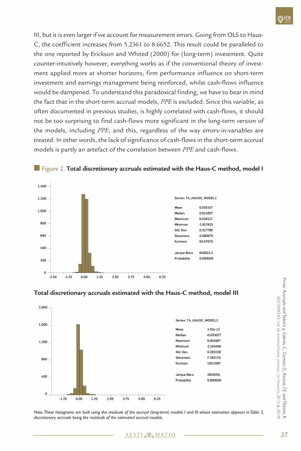
III, but it is even larger if we account for measurement errors. Going from OLS to Haus-
C, the coefficient increases from 5.2361 to 8.6652. This result could be paralleled tothe one reported by Erickson and Whited (2000) for (long-term) investment. Quite
counter-intuitively however, everything works as if the conventional theory of invest-
ment applied more at shorter horizons, firm performance influence on short-term
investment and earnings management being reinforced, whilst cash-flows influence
would be dampened. To understand this paradoxical finding, we have to bear in mind
the fact that in the short-term accrual models, PPE is excluded. Since this variable, asoften documented in previous studies, is highly correlated with cash-flows, it should
not be too surprising to find cash-flows more significant in the long-term version of
the models, including PPE, and this, regardless of the way errors-in-variables aretreated. In other words, the lack of significance of cash-flows in the short-term accrual
models is partly an artefact of the correlation between PPE and cash-flows.
n Figure 2. Total discretionary accruals estimated with the Haus-C method, model I
Total discretionary accruals estimated with the Haus-C method, model III
Note. These histograms are built using the residuals of the accrual (long-term) models I and III whose estimation appears in Table 3,discretionary accruals being the residuals of the estimated accrual models.
37
A E S T I T I OM A
firms’ a
ccruals and tobin’s q. Calm
ès, C., Cormier, D
., Racicot, F.E. and Théoret, R.a
estim
at
io, t
he
iebin
ter
na
tio
na
ljo
ur
na
lo
ffin
an
ce, 2013. 6
: 20-49
0
200
400
600
800
1,000
1,200
1,400
-2.50 -1.25 0.00 1.25 2.50 3.75 5.00 6.25
Mean 0.055157
Median 0.014857
Maximum 6.046117
Minimum -2.617825
Std. Dev. 0.317796
Skewness 5.080679
Kurtosis 83.07070
Jarque-Bera 840922.4
Probability 0.000000
Series: TA_HAUSC_MODEL1
0.0
0.0
6.0
0.3
5.0
8
0
400
800
1,200
1,600
2,000
-1.25 0.00 1.25 2.50 3.75 5.00 6.25
Mean 4.52e-12
Median -0.033077
Maximum 6.601697
Minimum -2.104556
Std. Dev. 0.283228
Skewness 7.282170
Kurtosis 150.0397
Jarque-Bera 2818250.
Probability 0.000000
Series: TA_HAUSC_MODEL3

n Figure 3. Current discretionary accruals estimated with the Haus-C method, model I
Current discretionary accruals estimated with the Haus-C method, model III
Note. These histograms are built using the residuals of the accrual (short-term) models I and III, whose estimation appears in Table 4,discretionary accruals being the residuals of the estimated accrual models.
n 5. Accruals Residuals Analysis
The problem with the residuals of the accrual models used to forecast stock returns is
that discretionary accruals do not necessarily reflect earnings management only, since
accruals are also related to firm performance. Consequently, differences in estimated
discretionary ac-cruals can be due to performance characteristics rather than incentives
to manage earnings — particularly so if the relationship between accruals and
performance is nonlinear. Given the significant role played by firm performance, our
motivation to consider accruals as a form of investment appears quite natural. In this
respect, the main contribution of this study is to show that Tobin’s q, a key explanatoryvariable of firm investment, indeed strongly influences firms’ accruals. In this paper, we
rely on OLS but also Haus-C to estimate our Tobin’s q augmented accrual model,
38
A E S T I T I OM A
firm
s’ a
ccru
als
and
tobi
n’s
q. Ca
lmès
, C., C
orm
ier,
D., R
acico
t, F.E
. and
Thé
oret
, R.
aes
tim
at
io, t
he
ieb
int
ern
at
ion
al
jou
rn
al
of
fin
an
ce,
2013
. 6: 2
0-49
Series: CA_HAUSC_MODEL1
0
200
400
600
800
1,000
1,200
-4 -2 0 2 4 6 8 10
Mean 0.088412
Median 0.047000
Maximum 9.974600
Minimum -3.594500
Std. Dev. 0.444797
Skewness 8.542643
Kurtosis 176.6226
Jarque-Bera 2423523.
Probability 0.000000
0.0
0.0
6.0
0.3
5.0
8
0
400
800
1,200
1,600
2,000
-1.25 0.00 1.25 2.50 3.75 5.00 6.25
Mean 4.52e-12
Median -0.033077
Maximum 6.601697
Minimum -2.104556
Std. Dev. 0.283228
Skewness 7.282170
Kurtosis 150.0397
Jarque-Bera 2818250.
Probability 0.000000
Series: TA_HAUSC_MODEL3

arguing that it delivers a robust fit of firms’ accruals. Logically, we should then expect
that this type of specification is also able to deliver residuals which can isolate the
earnings management component of discretionary accruals. As a robustness check, it
is thus instructive to study the residuals of our regressions — i.e., the discretionary part
of accruals.
From an econometric perspective, the mean of the residuals of a regression ought to
be equal to 0 in order to avoid any bias in the estimation. In this respect, TDA, totaldiscretionary accruals, also ought to be 0 in the long-run since no earnings
management practice can influence financial results indefinitely (Ronen and Yaari,
2008). Figure 2 and Figure 3 provide the distributions of total discretionary accruals,
TDA, and current discretionary accruals, CDA, respectively, both expressed in termsof total assets for models I and III. Compared to model I, model III seems to perform
better along this dimension. Indeed, in Figure 2, note that the mean of TDA is equalto 0.0558 when estimated with model I, whereas it is practically 0 when estimatedwith model III. Therefore, having a mean of zero, the TDA associated with model IIIseems appropriate to forecast returns. Relatedly, regardless of the model considered,
the TDA distribution seems positively skewed. For instance, for model III, the skewnesscoefficient is equal to 7.28, which supports the conventional view that discretionaryaccruals are likely influenced by various earnings management practices. As a matter
of fact, it is remarkable to see that, while the mean of model III residuals is lower, the
skewness of the residuals is actually higher. One obvious explanation is that, by
effectively controlling for firm performance, Tobin’s q is indeed able to isolate theearnings management information contained in discretionary accruals.
In other respects, as it is the case for TDA, the CDA mean goes down to 0 when theinvestment variables (cash flows and Tobin’s q) are introduced (Figure 3). As shownin Figure 3, the CDA mean for model I, at 0.088, is higher than the correspondingmean of TDA, and the CDA skewness coefficient, at 10.47, is much higher than itsTDA counterpart. This confirms that discretionary accruals are indeed manipulated,especially at short horizons9. A look at the skewness coefficient supports this view, as
the larger coefficient observed for model III (10.47 versus 8.54 for model I) suggeststhat the distribution of the residuals can no longer be attributable to firm
performance. Overall, our results suggest that the residuals of model III are well suited
for financial analysis because they appear purged from the systematic link between
stock returns and investment.
39
A E S T I T I OM A
firms’ a
ccruals and tobin’s q. Calm
ès, C., Cormier, D
., Racicot, F.E. and Théoret, R.a
estim
at
io, t
he
iebin
ter
na
tio
na
ljo
ur
na
lo
ffin
an
ce, 2013. 6
: 20-49
8 Remind that accruals are defined in terms of assets. 9 Accruals arise from a discrepancy of timing between cash-flows and the accounting recognition of the transaction. In this respect,accruals management is thus a short-term phenomenon which vanishes in the long-run. Over the firm’s lifetime, reported revenuesmust equal total cash inflows, and total accruals must equal zero (Ronen and Yaari, 2008).

n 6. Conclusion
Some econometric challenges are related to the estimation of our augmented accrual
model. A well-known issue relates to the difficulty of properly estimating Tobin’s q giventhat it is not directly observable. As usually done in the investment literature, we rely on
an average measure to proxy Tobin’s q. There is thus an inherent measurement errorrelated to the computation of this ratio. Ignoring the appropriate correction would
entail the usual empirical interaction between cash-flows and Tobin’s q, biasing theestimated coefficients of both variables. We thus resort to a specific estimation
procedure to tackle this measurement error. Based on this methodology, we are also
able to detect serious measurement errors in the basic accrual model and its augmented
versions. Our findings reveal that the differences between the coefficients obtained from
the IV method and those resulting from the standard OLS are actually quite substantial,
which suggests the presence of significant measurement errors in all variables.
More importantly, our main contribution is to show that Tobin’s q is a significant ex-planatory variable of firms’ accruals. Consistent with the literature on firm investment,
our results support the idea that financial constraints also influence accruals
management. However, we find that the impact of cash-flows is actually reduced when
simultaneously introducing Tobin’s q in the short-term version of the model. Clearly,this particular phenomenon is detectable with the IV estimation method we introduce.
Despite its merits, our study leaves many questions open to investigation. Accrual
models aim at analyzing the fundamental factors which normally influence cash-flows
smoothing in order to identify earnings management patterns with the residuals — i.e.,
with the discretionary accruals. With the introduction of Tobin’s q, we can derive“appropriate” estimated residuals, in the sense that they appear quite close to zero on
average. This is due to the fact that, given its theoretical property, Tobin’s q effectivelyremoves from accruals residuals the information related to firms’ performance. This
might prove particularly useful for portfolio managers and financial analysts, since
discretionary accruals provide an important information to forecast stocks returns.
However, compared to the alternative specifications provided in the literature (Wu
et al. 2007, 2010) we do not know a priori whether the residuals of the Tobin’s qaugmented model we propose are better suited to forecast stock returns. In this study,
our focus is to show that accruals can indeed be cast in terms of short-term investment.
Given the positive results we obtain, it will be interesting to investigate the relative
performance of our model vis-à-vis competing ones (e.g., Beneish, 1997) to forecast
stock market returns. Considering the nonlinear relationship between accruals and
firm performance, the autoregressive behavior of accruals, and the skewness
coefficients we obtain, it would be interesting to address this question using a GARCH
framework. This is left for future work.
40
A E S T I T I OM A
firm
s’ a
ccru
als
and
tobi
n’s
q. Ca
lmès
, C., C
orm
ier,
D., R
acico
t, F.E
. and
Thé
oret
, R.
aes
tim
at
io, t
he
ieb
int
ern
at
ion
al
jou
rn
al
of
fin
an
ce,
2013
. 6: 2
0-49
n Acknowledgements
We would like to thank the Chaire d’information financière et organisationnelle (ESG-UQAM)
for its financial support, and Cheng Few Lee, Steven J. Kachelmeier, Mark A. Trombley
and Stephen Young for their valuable comments.
n References
n Abel, A. and Blanchard, O. (1983). An intertemporal equilibrium model of saving and investment,
Econometrica, 51, pp. 675-692.
n Adda, J. and Cooper, R. (2003). Dynamic Economics. MIT Press, Cambridge.
n Bartov, E., Gul, F.A. and Tsui, J.S.L. (2001). Discretionary-accrual models and audit qualifications,
Journal of Accounting and Economics, 30, pp. 421-452.
n Beneish, M.D. (1997). Detecting GAAP violations: Implications for assessing earnings management
among firms with extreme financial performance, Journal of Accounting and Public Policy, 16,
pp. 271-309.
n Blanchard, O.J. and Fischer, S. (1989). Lectures on Macroeconomics. MIT Press, Cambridge.
n Brown, J.R., Fazzari, S.M. and Petersen, B.C. (2009). Financing innovation and growth: cash-flow,
external equity, and the 1990s R&D boom, Journal of Finance, 64, pp. 151-185.
n Brown, J.R. and Petersen, B.C. (2009). Why has the investment-cash flow sensitivity declined
so sharply? Risining R&D and equity market developments, Journal of Banking & Finance, 33,
pp. 971-984.
nBurgstahler, D. and Dichev, I. (1997). Earnings management to avoid earnings decreases and Losses,
Journal of Accounting & Economics, 24, pp. 99-126.
n Calmès, C. (2004). Financial Market Imperfections and Investment: an Overview, Bank of Canada,
EconWPA, No. 0409031.
n Coën, A. and Racicot F.E. (2007). Capital asset pricing models revisited: Evidence from errors-in-
variables, Economics Letters, 95, pp. 443-450.
n Cormier, D., Magnan, M. and Morard, B. (2000). The Contractual and Value Relevance of Reported
Earnings in a Dividend-Focused Environments, European Accounting Review, 9, pp. 387-417.
n Dagenais, M.G. and Dagenais, D.L. (1997). Higher moment estimators for linear regression models
with errors in the variables, Journal of Econometrics, 76, pp. 193-221.
n Dechow, P. (1994). Accounting earnings and cash-flows as measures of firm performance, Journal
of Accounting and Economics, 18, pp. 3-42.
n Dechow, P.M. and Dichev, I.D. (2002). The quality of accruals and earnings: The role of accruals
estimation errors, The Accounting Review, 77, pp. 35-59.
41
A E S T I T I OM A
firms’ a
ccruals and tobin’s q. Calm
ès, C., Cormier, D
., Racicot, F.E. and Théoret, R.a
estim
at
io, t
he
iebin
ter
na
tio
na
ljo
ur
na
lo
ffin
an
ce, 2013. 6
: 20-49

n Dechow, P.M., Richardson, S.A. and Tuna, I.A. (2003). Why are earnings kinky? An examination of
the earnings management explanation, Review of Accounting Studies, 8, pp. 355-384.
n Dechow, P., Sloan, R. and Sweeny, A. (1995). Detecting earnings management, The Accounting
Review, 70, pp. 193-225.
n DeFond, M. and Park, C. (1997). Smoothing income in anticipation of future earnings, Journal of
Accounting and Economics, 23, pp. 115-139.
n DeGeorge, F., Patel, J. and Zeckhauser, R. (1999). Earnings Management to Exceed Thresholds,
Journal of Business, 72, pp. 1-33.
n Durbin, J. (1954). Errors in variables, International Statistical Review, 22, pp. 23-32.
n Erickson, T. and Whited, T.M. (2000). Measurement errors and the relationship between investments
and Q, Journal of Political Economy, 108, pp. 1027-1057.
n Erickson, T. and Whited, T.M. (2002). Two-step GMM estimation of the errors-in-variables model
using high-order moments, Econometric Theory, 18, pp. 776-799.
n Fama, E.F. and French, K.R. (2007). Dissecting anomalies, Working Paper, University of Chicago.
n Fazzari, S.M., Hubbard, R.G. and Petersen, B.C. (1988). Financing constraints and corporate
investment, Brookings Papers on Economic Activity, 1, pp. 141-195.
n Francis, J., LaFond, R., Olsson, P. and Schipper, K. (2005). The market pricing of accruals quality,
Journal of Accounting and Economics, 39, pp. 295-327.
n Fuller, W.A. (1987). Measurement error models, John Wiley & Sons, New York.
n Geary, R.C. (1942). Inherent relations between random variables, Proceedings of the Royal Irish
Academy, 47, pp. 23-76.
n Gilchrist, S. and Himmelberg, C.P. (1995). Evidence on the role of cash-flow for investment, Journal
of Monetary Economics, 36, pp. 541-572.
n Hansen, G. (1999). Bias and measurement error in discretionary accrual models, Working paper,
Pennsylvania State University.
n Hausman, J.A. (1978). Specification tests in econometrics, Econometrica, 46, pp. 1251-1271.
n Hayashi, F. (1982). Tobin’s marginal q and average q: a neoclassical interpretation, Econometrica,
50, pp. 215-224.
n Hirshleifer, D., Hou, K. and Teoh, S.H. (2009). Accruals, cash flows, and aggregate stock returns,
Journal of Financial Economics, 91, pp. 389-406.
n Hirshleifer, D., Hou, K., Teoh, S.H. and Zhang, Y. (2004). Do investors overvalue firms with bloated
balance sheets?, Journal of Accounting and Economics, 38, pp. 297-331.
n Hribar, P. and Collins, D. (2002). Errors in estimating accruals: implications for empirical research,
Journal of Accounting Research, 40, pp. 105-134.
n Ibrahim, S. (2009). The usefulness of measures of consistency of discretionary components
of accruals in the detection of earnings management, Journal of Business Finance and Accounting,
36, pp. 1087-1116.
42
A E S T I T I OM A
firm
s’ a
ccru
als
and
tobi
n’s
q. Ca
lmès
, C., C
orm
ier,
D., R
acico
t, F.E
. and
Thé
oret
, R.
aes
tim
at
io, t
he
ieb
int
ern
at
ion
al
jou
rn
al
of
fin
an
ce,
2013
. 6: 2
0-49

n Jones, J.J. (1991). Earnings management during import relief investigations, Journal of Accounting
Research, 29, pp. 193-228.
n Kang, S.H. (2005). A conceptual and empirical evaluation of accrual prediction models, Working
paper, SSRN147259.
n Kang, S.H. and Sivaramakrishnan, K. (1995). Issues in testing earnings management and an
instrumental variable approach, Journal of Accounting Research, 33, pp. 353-367.
nKendall, M.G. and Stuart, A. (1963). The Advanced Theory of Statistics. Vol.1. London: Charles Griffin.
nKothari, S.P. (2001). Capital markets research and accounting, Journal of Accounting and Economics,
31, pp. 105-231.
n Kothari, S.P., Leone, A.J. and Wasley, C.E. (2005). Performance matched discretionary accrual
measures, Journal of Accounting and Economics, 39, pp. 163-197.
n Larcker, D.F. and Rusticus, T. (2010). On the use of instrumental variables in accounting research,
Journal of Accounting and Economics, 49, pp. 186-205.
n Leuz, C., Nanda, D. and Wysocky, P. (2003). Earnings management and investor protection: An
international comparison, Journal of Financial Economics, 69, pp. 506-527.
n Lewbel, A. (1997). Constructing instruments for regressions with measurement error when
no additional data are available, with an application to patents and R&D, Econometrica , 65,
pp. 1201-1213.
n MacKinnon, J.G. (1992). Model specification tests and artificial regressions, Journal of Economic
Literature, 30, pp. 102-146.
nMalevergne, Y. and Sornette, D. (2005). Higher moments portfolio theory, capitalizing on behavioral
anomalies of stock markets, Journal of Portfolio Management, 31, pp. 49-55.
n Marquardt, C. and Wiedman, C. (2004). How are earnings managed? An examination of specific
accruals, Contemporary Accounting Research, 21, pp. 461-489.
n McNichols, M.F.(2002). Discussion of the quality of accruals and earnings: The role of accrual
estimation error, The Accounting Review, 77, pp. 61-69.
n McNichols, M.F. and Wilson, G.P. (1988). Evidence of earnings management from the provision for
bad debts, Journal of Accounting Research, 26, pp. 1-31.
nMeng, J.G., Hu, G. and Bai, J. (2011). Olive: A simple method for estimating betas when factors are
measured with errors, Journal of Financial Research, 34, pp. 27-60.
n Modigliani, F. and Miller, M. (1958). The cost of capital, corporation finance and the theory of
investment, American Economic Review, 48, pp. 261-297.
n Pal, M. (1980). Consistent moment estimators of regression coefficients in the presence of errors in
variables, Journal of Econometrics, 14, pp. 349-364.
n Peasnell, K., Pope, P. and Young, S. (2000). Detecting earnings management using cross-sectional
abnormal accrual models, Accounting and Business Research, 30, pp. 313-326.
43
A E S T I T I OM A
firms’ a
ccruals and tobin’s q. Calm
ès, C., Cormier, D
., Racicot, F.E. and Théoret, R.a
estim
at
io, t
he
iebin
ter
na
tio
na
ljo
ur
na
lo
ffin
an
ce, 2013. 6
: 20-49

n Pindyck, R.S. and Rubinfeld, D.L. (1998). Econometric Models and Economic Forecasts, 4th edition,
McGraw-Hill, New York.
n Racicot, F.E. and Théoret, R. (2012). Optimally weighting higher moment instruments to deal with
measurement errors in financial returns models, Applied Financial Economics, 22, pp. 1135-1146.
n Ronen, J. and Yaari, V. (2008). Earnings Management: Emerging Insights in Theory, Practice and
Research. Springer, New York.
n Royshowdhury, S. (2006). Earnings management through real activities manipulation, Journal of
Accounting and Economics, 42, pp. 335-370.
n Sloan, R.G. (1996). Do stock prices fully reflect information in accruals and cash flows about future
earnings?, The Accounting Review, 71, pp. 289-315.
n Spencer, D.E. and Berk, K.N. (1981). A limited information specification test, Econometrica, 49,
pp. 1079-1085.
n Teoh, S.H., Welch, I. and Wong, T.J. (1998a). Earnings management and the underperformance of
seasoned equity offerings, Journal of Financial Economics, 50, pp. 63-99.
n Teoh, S.H., Welch, I. and Wong, T.J. (1998b). Earnings management and the long-run market
performance of initial public offerings, Journal of Finance, 53, pp. 1935-1974.
n Theil, H. (1953). Repeated least-squares applied to complete equations systems. The Hague: Central
Planning Bureau (mimeo).
n Tobin, J. (1969). A general equilibrium approach to monetary theory, Journal of Money, Credit and
Banking, 1, pp. 15-29.
nWu, D.M. (1973). Alternative tests of independence between stochastic regressors and disturbances,
Econometrica, 41, pp. 733-750.
nWu, J.G., Zhang, L. and Zhang, X.F. (2007). The accrual anomaly: Exploring the optimal investment
hypothesis, NBER working paper series.
n Wu, J.G., Zhang, L. and Zhang, X.F. (2010). The q-theory approach to understanding the accrual
anomaly, Journal of Accounting Research, 48, pp. 177-224.
n Xie, H. (2001). The mispricing of abnormal accruals, The Accounting Review, 76, pp. 357-373.
n Yaari, H., DaDalt, P., Ronen, J. and Yaari, V. (2007). On accrual conundrum in earnings management
research, mimeo.
n Ye, J. (2006). Accounting accruals and tests of earnings management, Working paper, Baruch
College.
n Young, S. (1999). Systematic measurement error in the estimation of discretionary accruals:
An evaluation of alternative modelling procedures, Journal of Business Finance & Accounting, 26,
pp. 833-862.
n Zhang, X.F. (2007). Accruals, investment and the accrual anomaly, The Accounting Review, 82, pp.
1333-1363.
44
A E S T I T I OM A
firm
s’ a
ccru
als
and
tobi
n’s
q. Ca
lmès
, C., C
orm
ier,
D., R
acico
t, F.E
. and
Thé
oret
, R.
aes
tim
at
io, t
he
ieb
int
ern
at
ion
al
jou
rn
al
of
fin
an
ce,
2013
. 6: 2
0-49

n Appendix A: The Choice of Instruments10
Since accrual models present specification errors the condition of orthogonality is
generally violated and the estimators of the coefficients of the models are not unbiased
and consistent. To reduce the estimation biases in these coefficients, we thus regress,
in a first pass, the endogenous explanatory variables on instruments. The delicate part
is to judiciously choose these instruments. To deal with specification errors, Geary
(1942), Durbin (1954), Kendall and Stewart (1963), Pal (1980), Fuller (1987), and
more recently Dagenais and Dagenais (1997), Lewbel (1997) and Meng et al. (2011)
have proposed instruments based on higher moments and cumulants. Racicot and
Théoret (2012) generalize these instruments and apply them to financial models of
returns, testing and correcting specification errors in a GMM framework.
The set of new instruments we propose to build an estimator accounting for specifica-
tion errors (and more specifically measurement errors) is based on an optimal
combination of the estimators of Durbin (1954) and Pal (1980). Let us first assume
the following general form y = a+Xb , where y is the vector (n x 1) representing thedependent variable, here accruals, and X is the matrix (n x k) of the explanatoryvariables11. b is the (k x 1) vector of parameters to estimate. Assume also the existenceof specification errors in the explanatory variables which might create inconsistency
in the estimation of the b vector. To tackle this issue, Durbin (1954) proposes to use
as instruments the following product: x*x, where x is the X matrix of the explanatoryvariables expressed in deviation from the mean, and where the symbol * stands for the
Hadamard element by element matrix multiplication operator. In the same vein, Pal
(1980) introduces as instruments cumulants based on the third power of x instead ofthe squares. Combining these instruments, we obtain a new matrix of instruments Zbased on the cumulants and co-cumulants of x and y, these being the matrix X andthe vector y expressed in deviation from the mean. This Z matrix may be partitionedinto k vectors or series, i.e. Z =[z1 z2 ... zk].The vector z1, built with the first explanatory
variable, is the instrument of the first explanatory variable, and so on. We regress the
explanatory variables on this vector Z to obtain x :
x = Z(Z’Z)–1 Z’x (15)
Then the new optimal instrumentswc based on cumulants of the explanatory variables
are defined as:
wc = x – x = [ wc1 wc
2 ... wck ] (16)
45
A E S T I T I OM A
firms’ a
ccruals and tobin’s q. Calm
ès, C., Cormier, D
., Racicot, F.E. and Théoret, R.a
estim
at
io, t
he
iebin
ter
na
tio
na
ljo
ur
na
lo
ffin
an
ce, 2013. 6
: 20-49
10 See: Racicot and Théoret (2012).11 In model III of short-term accruals the matrix X is equal to [1/Ai ΔSalesi /Ai CFi qi/Ai].

In their study, Racicot and Théoret (2012) find that this kind of instruments appear
orthogonal to the estimated residuals. The correlation between wci and the
corresponding explanatory variable xi is around 90%, the correlation is close to 0 withthe other explanatory variables, and in this sense, these instruments can be considered
optimal. To improve the existing instrumental methods used to tackle the endogeneity
issue in accrual models, we adopt the wci instruments they developed with a modified
version of the Hausman (1978) artificial regression.
n Appendix B: The Augmented Hausman Artificial Regression12
To detect specification errors in our sample of firms, we could use the original Haus-
man h test13 with the following classical linear regression model: y = Xb+e, where y isa (n×1) vector representing the dependent variable; X, a (n×k) matrix of the explanatoryvariables; b, a (k×1) parameters vector, and e ~ iid (0,s2). The Hausman test compares
two estimates of the parameters vector, bOLS, the least-squares estimator (OLS), andbA, an alternative estimator taking a variety of specifications (the instrumental variables
estimator bIV in our case). The hypothesis H0 is the absence of specification errors,
and H1, their presence. First, note that the vector of estimates bIV is consistent under
both H0 and H1, whereas bOLS is only consistent under H0 and not consistent under
H1. Consequently, under H0, bIV is less efficient than bOLS. Second, the Hausman test
aims at verifying if “the endogeneity” of some variables – in our case the variables
measured with errors – has any significant effect on the estimation of the parameters
vector. Therefore, the Hausman test is an orthogonality test, that is, helping verify if plim
(1/T) X’e = 0 in large samples. To implement the test, researchers then define the follo-wing vector of contrasts or distances: bIV – bOLS . The resulting h test statistic reads:h=(bIV – bOLS)T [Var(bIV)–Var(bOLS)]–1(bIV – bOLS)~χ2 (g), with Var(bIV) and Var(bOLS) therespective estimates of the covariance matrices of bIV and bOLS , and g the number ofpotentially endogenous regressors. H0 is rejected if the p-value of this test is less thana, the critical threshold of the test (e.g. 5%).
Third, and more importantly, note that, according to MacKinnon (1992), the h testmight also run into difficulties if the matrix [Var(bIV)–Var(bOLS)], which weights thevector of contrasts, is not positive definite. Since this is the case with most of the
accrual models we study, we rely instead on an alternative method to run our Hausman
test. For example, assume a five variable linear regression model (e.g., the long-term
version of the accrual model incorporating Tobin’s q and cash-flows model III):
46
12 For previous applications of this method see Coën and Racicot (2007) and Racicot and Théoret (2012). 13 For details on the Hausman test, see: Hausman (1978), Wu (1973), MacKinnon (1992) and Pindyck and Rubinfeld (1998). A verygood presentation of the version of the Hausman test using an artificial regression in the context of correction of errors-in-variablesmay be found in Pindyck and Rubinfeld (1998). They present the case of one explanatory variable, whereas we apply it to the caseof multiple explanatory variables.
I N T E R N AT I O N A LJ O U R N A L O F F I N A N C E
A E S T I T I OM ATHE I E B
firm
s’ a
ccru
als
and
tobi
n’s
q. Ca
lmès
, C., C
orm
ier,
D., R
acico
t, F.E
. and
Thé
oret
, R.
aes
tim
at
io, t
he
ieb
int
ern
at
ion
al
jou
rn
al
of
fin
an
ce,
2013
. 6: 2
0-49

yt= b0+5
∑i=1
bi x*it +et (17)
with e ~ iid (0,s 2).
and that the variables x*it 14 are measured with errors, that is:
xit = x*it+uit (18)
with xit the corresponding observed variables measured with errors. By substituting
Equation (18) in Equation (17), we have:
yt =b0+5
∑i=1
bi xit +e*t (19)
with e*t = et –5∑i=1
bi uit . As explained before, estimating the coefficients of Equation (19)
by the OLS method leads to biased and inconsistent coefficients because the expla-
natory variables are correlated with the innovation. Consistent estimators can be found
if we can identify an instrument vector zt which is correlated with every explanatory
variable but not with the innovation of Equation (19). Then we regress the five
explanatory variables on zt . We have:
xit = xit +wit =gi zt+wit (20)
where xit is the value of xit estimated with the vector of instruments, and wit the residuals
of the regression of xit on xit . Substituting Equation (20) into Equation (19), the
following artificial regression obtains:
yt =b0+5
∑i=1
bi xit +5
∑i=1
bi wit +e*t (21)
The explanatory variables of this equation are, on the one hand, the estimated values
of xit , obtained by regressing the five variables on the vector of instruments zt , and, on
the other hand, the respective residuals of these regressions. Therefore, Equation (21)
is an augmented version of Equation (19).
We can show that:
p lim[ ]= p lim[ ]= –bis2ui (22)
If there is no specification error, s 2ui =0, the OLS estimation results in a consistent
estimator for b1 , the parameter of wit in Equation (21), and the coefficient is then
47I N T E R N AT I O N A L
J O U R N A L O F F I N A N C E
A E S T I T I OM ATHE I E B
firms’ a
ccruals and tobin’s q. Calm
ès, C., Cormier, D
., Racicot, F.E. and Théoret, R.a
estim
at
io, t
he
iebin
ter
na
tio
na
ljo
ur
na
lo
ffin
an
ce, 2013. 6
: 20-4914 We use the asterisks to designate the unobserved variables.
∑wit+e*t
N–b1∑xituit
N
equal to the one of the corresponding explanatory variable. In the case of specification
errors, s 2ui ≠ 0 and, therefore, the estimator is not consistent. For detecting the presence
of specification errors, as we do not know a priori if there are such errors, we first have
to replace the coefficients of the wit in Equation (20) by θi . We thus have:
yt =b0+5
∑i=1
bi xit +5
∑i=1
θi wit +e*t (23)
Since according to Equation (20), xit = xit – wit , we can then rewrite Equation (23) as:
yt =b0+5
∑i=1
bi xit +5
∑i=1
(θi –bi )wit +e*t (24)
If there is no specification error for xit , then θi = bi . In the opposite case, θi ≠ bi , and
the coefficients of the residuals terms wit are significantly different from 0. Asignificantly positive estimate of (θi –bi) indicates that the estimated coefficient of thecorresponding explanatory variable, xit , is overstated in the OLS regression. In this
case, the estimated coefficient for this variable is lower compared to the OLS one in
Equation (24). On the other hand, if the estimated coefficient (θi –bi ) is significantlynegative, it suggests that the estimated coefficient of the corresponding explanatory
variable, xit , is understated by OLS, and consequently the estimated coefficient for this
variable is higher in Equation (24). In other respects, the estimated coefficients bi are
identical to those produced by a TSLS procedure with the same instruments (Spencer
and Berk, 1981), except that, compared to a strict TSLS, Equation (24) also provides
additional information which proves quite helpful when estimating accruals. In the
procedure we propose to test for specification errors, we first regress the observed
explanatory variables xit on the instruments vector to obtain the residuals wit . Then,
we regress yt on the observed explanatory variables xit and on these residuals wit . This
is the auxiliary (or artificial) regression we just described. If the coefficient of the
residuals associated with an explanatory variable is significantly different from 0, wecan directly infer the presence of a specification error. In this case, a t test is used toassess the severity of the specification error. To our knowledge, such a test has never
been used in this context. Usually, a Wald test (F test) is performed to check whetherthe whole set of (θi –bi) coefficients is significantly different from zero, but this ignoresthe case of specification errors associated with a specific subset of explanatory variables.
We can generalize the former procedure to the case of k explanatory variables with ourmodified Hausman regression. Let X be a (n xk) matrix of explanatory variables notorthogonal to the innovation, and let Z be a (n x s) matrix of instruments (s>k). Weregress X on Z to obtain X :
X=Zθ= Z(Z’Z)–1 Z’X=Pz X (25)
where Pz is the “predicted value maker”. Having run this regression, we can compute
the matrix of residuals w :
48I N T E R N AT I O N A L
J O U R N A L O F F I N A N C E
A E S T I T I OM ATHE I E B
firm
s’ a
ccru
als
and
tobi
n’s
q. Ca
lmès
, C., C
orm
ier,
D., R
acico
t, F.E
. and
Thé
oret
, R.
aes
tim
at
io, t
he
ieb
int
ern
at
ion
al
jou
rn
al
of
fin
an
ce,
2013
. 6: 2
0-49

w =X–X=X –Pz X = (I –Pz)X (26)
and perform the following artificial regression:
y =X b+wl (27)
A F test on the l coefficients indicates whether the w are significant as a group, butwe also introduce a t test on each individual coefficient to check whether thecorresponding b is understated or overstated. The vector of b estimated in Equation
(27) is identical to the TSLS estimates, that is:
b= bIV =(X’Pz X)–1 X’Pz y (28)
n
49I N T E R N AT I O N A L
J O U R N A L O F F I N A N C E
A E S T I T I OM ATHE I E B
firms’ a
ccruals and tobin’s q. Calm
ès, C., Cormier, D
., Racicot, F.E. and Théoret, R.a
estim
at
io, t
he
iebin
ter
na
tio
na
ljo
ur
na
lo
ffin
an
ce, 2013. 6
: 20-49