Embed Size (px)
Citation preview
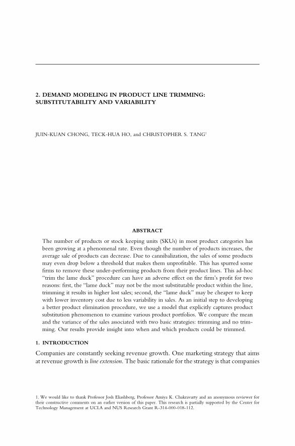
2. DEMAND MODELING IN PRODUCT LINE TRIMMING:SUBSTITUTABILITY AND VARIABILITY
JUIN-KUAN CHONG, TECK-HUA HO, and CHRISTOPHER S. TANG1
ABSTRACT
The number of products or stock keeping units (SKUs) in most product categories hasbeen growing at a phenomenal rate. Even though the number of products increases, theaverage sale of products can decrease. Due to cannibalization, the sales of some productsmay even drop below a threshold that makes them unprofitable. This has spurred somefirms to remove these under-performing products from their product lines. This ad-hoc“trim the lame duck” procedure can have an adverse effect on the firm’s profit for tworeasons: first, the “lame duck” may not be the most substitutable product within the line,trimming it results in higher lost sales; second, the “lame duck” may be cheaper to keepwith lower inventory cost due to less variability in sales. As an initial step to developinga better product elimination procedure, we use a model that explicitly captures productsubstitution phenomenon to examine various product portfolios. We compare the meanand the variance of the sales associated with two basic strategies: trimming and no trim-ming. Our results provide insight into when and which products could be trimmed.
1. INTRODUCTION
Companies are constantly seeking revenue growth. One marketing strategy that aimsat revenue growth is line extension. The basic rationale for the strategy is that companies
1. We would like to thank Professor Josh Eliashberg, Professor Amiya K. Chakravarty and an anonymous reviewer fortheir constructive comments on an earlier version of this paper. This research is partially supported by the Center forTechnology Management at UCLA and NUS Research Grant R-314-000-018-112.
40 I. New products and existing product portfolio management
can increase their revenue if they cater to the diverse preferences of the consumersin the product categories. This strategy is perceived to be less risky since line extensionsare launched in an existing product category that already has an established customerbase. The wide-spread practice of this strategy has led to an unprecedented increasein the number of stock keeping units (SKUs) in most product categories (see forexample Hays (1994), Khermouch (1995), Putsis and Bayus (2001)).
There are several criticisms of the line extension strategy. Bayus and Putsis (1999)show that line extension can significantly increase costs and the cost increase dwarfsthe benefits derived from the increase in revenue. Quelch and Kenny (1994) suggestedthat many companies fail to account for the hidden costs of product proliferationassociated with line extension. Perhaps, more critically, these authors challenged thewisdom “more products, more revenues” by arguing that “people do not eat more,drink more, brush their teeth more, or wash their hair more just because they havemore products from which to choose.” In fact, they showed that the total sales ofmany product categories (such as cookies and shampoo) decreased despite a significantincrease in the number of products. This argument seems plausible for certain matureproduct categories where growth is often minimal or stagnant.
Quelch and Kenny’s finding suggests that increasing the number of SKUs in aproduct category does not necessarily draw new customers to the category. Conse-quently, sales of new products must come from the cannibalization on the sales ofexisting products. This happens especially when the existing products are similar orinferior to the new extensions. This has prompted some companies to trim theirproduct lines (e.g. Khermouch (1995)). There are several rationales for product linetrimming. Firstly, the sales of some products can drop below a level which makes itunprofitable for firms to continue supplying them. Secondly, intense competition forlimited grocery shelf space drives firms to remove the under-performing products,giving ‘space’ to more promising new products. In most cases, the companies tendto trim their product line in a reactive manner. Product obsolescence can be a causeof such reaction. Avlonitis and James (1982) reported, in a survey of 94 firms, thatmost firms trimmed their product lines because of product obsolescence. Factors con-tributing to product obsolescence include change in government regulations, changeof buyers’ specification, and development of new products. In a mail survey of 166companies, Hart (1988) concluded that firms also trimmed their product lines becauseof other factors such as resource shortage, poor product quality, rationalization dueto merger and acquisition, and problems associated with raw materials.
On the proactive side, firms might want to trim their product lines for two reasons.First, a leaner product line enables a firm to regain its product focus. Some reportssuggest that an over-crowded product category can lead to brand loyalty weakening(see for example Hays (1994) and Narisetti (1997)). This brand weakening phenome-non makes the product category very competitive because customers are easily swayedby price promotion (c.f. Quelch and Kenny (1994)). Second, a leaner product lineallows a firm to streamline its manufacturing and logistics functions. This is particularlyuseful when product trimming has only a minimal or no impact on the sales of thefirm’s entire product line. Indeed, a study conducted by the Food Marketing Institute
2. Demand modeling in product line trimming: substitutability and variability 41
found that the retailers can reduce the number of SKUs by up to 25% without hurtingsales or consumers’ perception of variety (c.f. Teinowitz and Lawrence (1993)). How-ever, trimming the wrong product can be costly. For instance, the removal of ClassicCoke by Coca Cola Company in 1985 caused a strong negative reaction by its consum-ers. Consequently, the company had to re-introduce the product to reduce the lossof customer to its competitors.
Despite its strategic importance, empirical evidence has shown that most companiesdo not have a formal product elimination program. Hise and McGinnis (1975) re-ported that only 31.3% out of their sample of 96 firms have formal procedures. Hiseet al. (1984) observed a similar pattern: 120 out of a sample of 299 firms have productelimination programs. But only 31% of the 120 firms have a documented program.A survey of U.S. and U.K. firms indicated that less than half of the sample ever utilizeany formal methodology in making product elimination decision (c.f. Greenley andBayus (1994)). The formality of a product elimination program appears to correlatewith its frequency of use. In a sample size of 94 firms, Avlonitis (1985) observed thatthe more products a firm trims, the more formal the process gets; and that the longerit takes to trim a product, the less formal the process is. Because of the rapid rise of thenumber of SKU, we expect product trimming to receive more managerial attention inthe near future. The need to formalize product trimming process can not be over-emphasized.
A formal procedure for product line trimming must address the following twofundamental questions: (1) Given the current line of products, should the firm trimits product line? (2) Suppose it is desirable to trim the product line, which product(s)should be eliminated? Several approaches were suggested in earlier works (see forexample, Berenson (1963), Alexander (1964), Kotler (1965), Hamelman and Mazze(1972), Browne and Kemp (1976)). Most of these approaches use a rating scheme torate the attractiveness of the products. Berenson (1963) based his model on five deci-sion factors, namely, financial security, financial opportunity, marketing strategy, so-cial responsibility and organized intervention. Management assigns weight to eachfactor to reflect its relative importance. The summation of five weighted scores be-comes the overall rating of a product. Alexander (1964) used a similar procedure witha different set of factors. These are sales trend, price trend, profit trend, substituteproducts, product effectiveness and demand on executive time. Kotler (1965) did notprovide a list of factors to consider. Instead, he suggested a six-step procedure wherethe first 3 steps were used by management to develop a comprehensive set of criteriaand to generate ratings and weights for these criteria. A “product retention index”,which is computed in a similar fashion as those of Berenson (1963) and Alexander(1964), is calculated for each product using the ratings and weights. A different indexwas suggested by Hamelman and Mazze (1972). Their “Selection Index Number(SINi)” is a ratio of the square of product i’s percentage contribution margin to itspercentage resource cost utilization. Browne and Kemp (1976) suggested a generalmultiple stage sequential review process. First, weak products are detected based oncriteria specified by top management. Further analysis and evaluation of these productsare done leading to an elimination decision and finally implementation.
42 I. New products and existing product portfolio management
These models are “macro” in the sense that they do not capture consumer choiceprocess and product substitution explicitly. But both components are vital to an accu-rate assessment of the impact due to trimming. Knowing which products consumerswill switch to in the absence of a product allows one to quantify precisely the impactof trimming. Our model incorporates the consumer choice process and product substi-tution phenomenon explicitly.
The intent of this paper is to highlight the importance of product substitutabilityand to examine its impact on product line trimming in terms of expected demand anddemand variability. Urban (1969) studies the impact of product substitutability on themarketing strategy of a product line. Specifically, Urban (1969) models consumerresponse to different marketing mixes of a product line and use it to determine anoptimal allocation of marketing mix for each product in a product line. In this work,we model consumer response to the removal of a product from a product line anduse it to evaluate product trimming decisions.
There are several product portfolio models that incorporate, whether explicitly orimplicitly, the expected demand (i.e. return) and demand variability (i.e. risk) in theiranalyses. These models either assimilate the financial portfolio analysis in their ap-proaches (e.g. Mahajan and Wind (1985), Mahajan, Wind and Bradford (1982))oruse a mathematical programming formulation in their analyses (e.g. Larreche and Srin-ivasan (1982), Corstjens and Weinstein (1982)). The prime objective of these modelsis to determine the right product lines in the optimal product portfolio and to allocatemarketing resources to these product lines. Our work is complementary to these mod-els. We focus our analysis on the impact of product trimming on the expected demandand the variance of demand for the remaining products. The result of our analysiscan potentially be used as an input to these optimization models.
One might argue that an alternative strategy to product line trimming is to lowerthe price of under-performing products.2 However, this strategy may not be desirable(or even viable) for the following reasons. First, the products may differ only in prod-uct attributes such as taste (e.g. fruit drops), flavor (e.g. ice cream) or color (e.g. T-shirts, ball pen). The consumers do not usually expect any price difference in suchcases. Second, the manufacturer may have limited freedom to charge different pricesfor similar products because this may not be acceptable to the retailers and consumers.For example, we can not price a product below another product having less featureor of a smaller package size. Third, in industries where the production lead time isrelatively long, product line decision must precede pricing decision. Hence, we focuson product line decision.
To analyze the underlying issue whether to trim or not, we consider a situationin which a firm must select one of the following strategies: Same Line (i.e., no productsshould be eliminated from the line) and Trim Line (i.e., some products should be
2. Instead of price decrease, one might suggest price increase to realize a higher profit margin. This is a less viable optionsince sales volume tends to be low for the under-performing products.
2. Demand modeling in product line trimming: substitutability and variability 43
eliminated from the line). Specifically, we analyze and compare the expected sales (ordemand) and the variance of the sales associated with the two strategies. Besides ex-pected demand, we analyze the variance of the demand, a variable commonly treatedas noise by marketing scientists but studied extensively by operations researchers (seeSilver and Peterson (1985)), because it is a good surrogate for the manufacturing andlogistics costs. We present a simple framework that enables brand managers to betterconceptualize the impact of product trimming. In this framework, we specify condi-tions under which the Same Line strategy is optimal. In the event that the Trim Linestrategy may be optimal, our model suggests potential candidates to be trimmed fromthe line. Driven by its intuitive appeal, many firms tend to adopt the so-called lameduck heuristic: trim the product that has the lowest sales (see surveys by Hart (1988),and Avlonitis and James (1982)). We shall show later that this heuristic can be sub-optimal because it neglects demand interaction among products within the same cate-gory.
This paper is organized as follows. In the next section, we present a model thatcaptures substitutability among products. Section 3 compares the ‘Same Line’ and‘Trim Line’ strategies. In addition, we derive conditions under which the Same Linestrategy is optimal. Section 4 deals with the situations when the Trim Line strategymay be optimal. We shows why and when the “lame duck” heuristic can be seriouslyflawed. In section 5, we provide a numerical example to illustrate some of the insightsgenerated from our analysis. Section 6 concludes the paper with some suggestions forfuture research.
2. THE MODEL
Consider a firm that manufactures and sells a line of N products in a selling season.The firm has accumulated some experience in selling the N products during previousseasons. At the beginning of the current season, the firm is contemplating if certainproducts should be removed from the product line. Essentially, the firm can eitheroffer the same N products (i.e., adopt ‘Same Line’ strategy) or trim the line by remov-ing some products (i.e., adopt ‘Trim Line’ strategy). In the event that the Trim Linestrategy is preferred, the firm would like to determine the product(s) to be eliminatedfrom the product line. In order to evaluate the pros and cons of the Same Line andTrim Line strategies, one needs to examine the impact of each strategy on the expectedsales (or demand) and the variance of demand of the products must be determined.This observation motivates us to develop a simple model that captures the consumerpurchasing processes and product substitution.
In our model, the product category has N � 1 products indexed by i where i �0, 1, . . . , N � 1, N. For expository purpose, we aggregate all other products otherthan those of the firm and denote this ‘aggregated product bundle’ as product 0.Products 1 to N constitute the firm’s product line before line trimming. The productcategory consists of a population of consumers with heterogeneous product prefer-ences. Each consumer is assumed to have a stationary and zero-order probabilisticproduct choice process. We consider the case in which the consumers are broadly
44 I. New products and existing product portfolio management
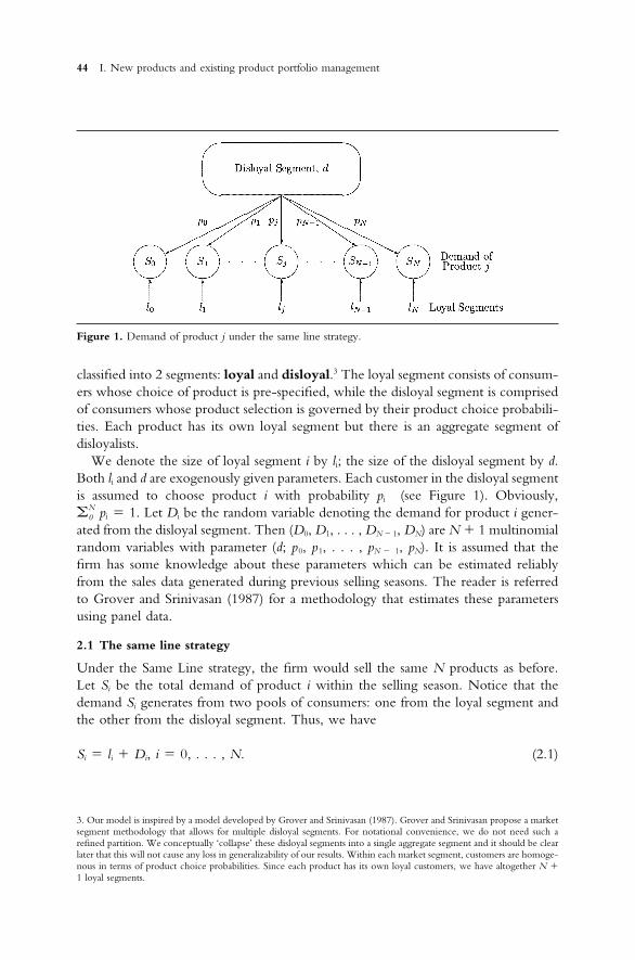
Figure 1. Demand of product j under the same line strategy.
classified into 2 segments: loyal and disloyal.3 The loyal segment consists of consum-ers whose choice of product is pre-specified, while the disloyal segment is comprisedof consumers whose product selection is governed by their product choice probabili-ties. Each product has its own loyal segment but there is an aggregate segment ofdisloyalists.
We denote the size of loyal segment i by li; the size of the disloyal segment by d.Both li and d are exogenously given parameters. Each customer in the disloyal segmentis assumed to choose product i with probability pi (see Figure 1). Obviously,�N
0 pi � 1. Let Di be the random variable denoting the demand for product i gener-ated from the disloyal segment. Then (D0, D1, . . . , DN � 1, DN) are N � 1 multinomialrandom variables with parameter (d; p0, p1, . . . , pN � 1, pN). It is assumed that thefirm has some knowledge about these parameters which can be estimated reliablyfrom the sales data generated during previous selling seasons. The reader is referredto Grover and Srinivasan (1987) for a methodology that estimates these parametersusing panel data.
2.1 The same line strategy
Under the Same Line strategy, the firm would sell the same N products as before.Let Si be the total demand of product i within the selling season. Notice that thedemand Si generates from two pools of consumers: one from the loyal segment andthe other from the disloyal segment. Thus, we have
Si � li � Di, i � 0, . . . , N. (2.1)
3. Our model is inspired by a model developed by Grover and Srinivasan (1987). Grover and Srinivasan propose a marketsegment methodology that allows for multiple disloyal segments. For notational convenience, we do not need such arefined partition. We conceptually ‘collapse’ these disloyal segments into a single aggregate segment and it should be clearlater that this will not cause any loss in generalizability of our results. Within each market segment, customers are homoge-nous in terms of product choice probabilities. Since each product has its own loyal customers, we have altogether N �1 loyal segments.
2. Demand modeling in product line trimming: substitutability and variability 45
It follows from (2.1) and the properties of multinomial random variables that theexpected value and the variance of Si can be expressed as:
E (Si ) � li � dpi, i � 0, . . . , N,Var (Si) � dpi (1 � pi ), i � 0, . . . , N.
In this case, it is easy to check that the mean and variance of the total demand ofall products in the firm’s product line under the Same Line strategy are given by:
E ��N
1Si� � �
N
j � 1lj � d(1 � p0) (2.2)
and,
Var ��N
1Si� � d p0 (1 � p0). (2.3)
2.2 The trim line strategy
Suppose that the firm has decided to trim product i from its product line. Then thereare N � 1 remaining products in the line, namely, 1, . . . , i � 1, i � 1, . . . , N.In this paper, we shall assume that the elimination of product i would have direct impacton the purchasing behavior of two specific groups (the loyal segment of product iand the disloyal segment) as follows:
2.2.1 The loyal segment of product i
When we eliminate product i from the product line, the customers in loyal segment of producti have to consider other alternatives. Each of these li customers may consider the followingalternatives: (1) becomes loyal to other products; (2) joins the disloyal segment and selects theproduct according to some choice probabilities; or (3) becomes disenchanted and leaves theconsumer base. Thus, for each customer who belongs to the loyal segment i, it is assumed thatthere is a probability qij that he/she becomes ‘loyal’ to product j, where j � 0,1, . . . , i � 1,i � 1, . . . , N, that there is a probability xi that he/she joins the disloyal group, and that thereis a probability yi that he/she leaves the consumer base. Clearly, �j ≠ i qij � xi � yi � 1, fori � 1, . . . , N.
Notice that the values of qij, xi, yi depend on the nature of product i and the degree of itssubstitutability with other products in the category.4 When there exists a highly substitutable
4. Substitution between products can occur because products are often similar to some degree. Thus, when a product isnot available for purchase, some customers may instead buy an alternative product. Intuitively, one would expect productsubstitution to occur more readily between a pair of similar products than between a pair of dissimilar products. Thisnotion of similarity is implicit in most product positioning models; products that are positioned close to each other inthe perceptual space are more similar to each other and are more easily substitutable (see Green and Krieger, 1993). Inthe classical attraction model (Bell, Keeney and Little, 1975), when a product i is eliminated from the consideration andchoice set, the probability for product j (j ≠ i) is increased from Aj/�Ak
k to Aj/�Akk ≠ i where Ak is the level of attraction
of product k. Thus, the attraction model restricts that the ratio of the purchase probabilities of any two remaining productsstays constant. This restriction is not required in our model.
46 I. New products and existing product portfolio management
product j, it is reasonable to assume that qij � 1, and {qik, k ≠ j }, xi, yi � 0. Notice that thesubstitutable product j could be one of the remaining products (i.e., j � 1, . . . , i � 1, i �1, . . . , N), or it could be one of the products that belongs to the competitors (i.e., when j� 0). However, when all other products are equally substitutable, customers may join thedisloyal group (i.e., xi � 1). Finally, when the salient features of product i are not captured inother products, it is possible that the i’s loyal consumers may leave the product category com-pletely (i.e., yi � 1).5
Let Lij be the size of the loyal segment j generated from the loyal segment li if thefirm eliminates product i. Let Xi be the new addition to the disloyal segment generatedfrom the loyal segment li after trimming product i. Let Yi be the number of customerswho leave the product category. In this case, it is easy to see that the random variables(Li0, . . . , Li,i � 1, Li,i � 1, . . . , LiN, Xi, Yi) are N � 2 multinomially distributed withparameters (li; qi0, . . . , qi,i � 1, qi,i � 1, . . . , qiN, xi, yi).
2.2.2 The disloyal segment
There are two disloyal segments that are affected by the elimination of product i. These twodisloyal segments are: Di, the original disloyal segment who intends to buy product i, and Xi,the new addition to the disloyal segment generated from the loyal segment li after trimmingproduct i. Depending on its substitutability with each of the remaining products j, it is assumedthat each consumer who belongs to these two disloyal segments will ‘switch’ to product j withprobability αij.6 Notice that �N
j � 0, j ≠ i αij � 1. Let Dij be the random variable denoting thedemand for product j generated from the original disloyal segment after trimming product ifrom the product line. Then {Dij : j � 0, . . . , i � 1, i � 1, . . . , N } are N multinomialrandom variables with parameters (Di; αi0, αi1, . . . , αiN). Similarly, let Xij be the random variabledenoting the demand for product j generated from the additional disloyal segment coming fromthe loyal segment of product i. Then {Xij : j � 0, . . . , i � 1, i � 1, . . . , N } are N multinomialrandom variables with parameters (Xi ; αi0,αi1, . . . , αiN).
By considering the impact of trimming product i on the loyal segment of producti and the disloyal segment, the effective demand of product j under the Trim Linestrategy can be expressed as:
Tij � lj � Lij � Dj � Dij � Xij , j � 0, 1, . . . , i � 1, i � 1, . . . , N.
Notice that the total demand Tij for product j is the sum of the various loyal anddisloyal segments. The loyal segment consists of the old loyal segment of product j,lj , and the new addition of loyal segment generated from a migration from the loyalsegment of i, Lij . The disloyal segment consists of the existing disloyal segment, Dj ,the substitution from the existing disloyal segment of product i, Dij , and the substitu-
5. The elimination of ‘Classic Coke’ is such a case when many consumers have threatened Coca-Cola company that theywill abandon cola drinks and switch to other types of soda.6. To simplify the exposition of our model, we assume that the ‘switching’ probabilities are the same for both disloyalsegments; however, our analysis can be easily extended to the case when these probabilities are different.
2. Demand modeling in product line trimming: substitutability and variability 47
Figure 2. Demand of product j with product i trimmed.
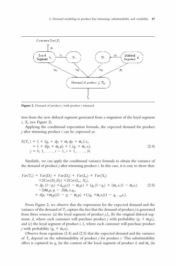
tion from the new disloyal segment generated from a migration of the loyal segmenti, Xij (see Figure 2).
Applying the conditional expectation formula, the expected demand for productj after trimming product i can be expressed as:
E(Tij ) � lj � liqij � dpj � αij dpi � αij li xi,� lj � d(pj � αij pi) � li (qij � αij xi), (2.4)
j � 0, 1, . . . , i � 1, i � 1, . . . , N.
Similarly, we can apply the conditional variance formula to obtain the variance ofthe demand of product j after trimming product i. In this case, it is easy to show that:
Var (Tij ) � Var (Dj ) � Var (Dij ) � Var (Lij ) � Var (Xij )�2Cov (Dj ,Dij ) �2Cov (Lij , Xij ),
� dpj (1�pj ) �dαij pi (1 � αij pi ) � liqij (1�qij ) � liαij xi (1 � αijxi ) (2.5)�2dαij pi pj � 2liαij xi qij ,
� d(pj �αijpi)(1 � pj � αij pi) �li (qij �αijxi)(1 � qij � αijxi ).
From Figure 2, we observe that the expressions for the expected demand and thevariance of the demand of Tij capture the fact that the demand of product j is generatedfrom three sources: (a) the loyal segment of product j,lj, (b) the original disloyal seg-ment, d, where each customer will purchase product j with probability (pj � αijpi),and (c) the loyal segment of product i, li, where each customer will purchase productj with probability (qij � αijxi).
Observe from equations (2.4) and (2.5) that the expected demand and the varianceof Tij depend on the substitutability of product j for product i. This substitutabilityeffect is captured in qij (in the context of the loyal segment of product i) and αij (in
48 I. New products and existing product portfolio management
the context of the disloyal segment). To examine the expectation and the varianceof the demand for the remaining product line (i.e., �N
j �1, j ≠iTij), if we trim product ifrom the line, observe that:
�N
j �l , j ≠ i
Tij � �N
j �1, j ≠ i
{lj � Dj � Dij � Lij � Xij},
� �N
j �1
lj � d � D0 � Li0 � Di0 � Xi0 � Yi.
By applying (2.4) and (2.5), it can be easily shown that:
E� �N
j � 1, j ≠ i
Tij� � �N
j �1
lj � d(1 � p0) � {αi0pi � li(qi0 � αi0xi � yi)}. (2.6)
and
Var� �N
j � 1, j ≠ i
Tij� � dp0(1 � p0) � dαi0pi(1 � αi0pi)� 2dαi0pip0 � liqi0(1 � qi0)� liαi0xi(1 � αi0xi) � liyi(1 � yi)� 2liqi0yi �2liqi0αi0xi � 2liyiαi0xi,
which can be simplified into:
Var� �N
j �1, j ≠i
Tij� � d(p0 � αi0pi)(1 � p0 � αi0pi) (2.7)� li(yi � qi0 � αi0xi)(1 � yi � qi0 � αi0xi).
3. SAME LINE VS. TRIM LINE STRATEGIES
In the last section, we derived the expressions for the expectation and the varianceof the demand of the entire product line under the same line and trim line strategies(i.e. (2.2), (2.3), (2.6) and (2.7)). In this section, we develop a simple framework forcomparing the Same Line and Trim Line strategies. Under the framework, the prosand cons associated with each of the strategies can be represented as a point on a two-dimensional map. The two dimensions on this map are the expected demand of theentire product line (vertical axis) and the variance of the demand of the entire productline (horizontal axis). The justification of this two-dimensional map is as follows.Observe that the expected revenue increases in expected demand, and that the ex-pected costs (processing cost, production and capacity planning cost, and inventorycost) increases in the variance of the demand (The reader is referred to Silver andPeterson (1984) for an excellent discussion on how costs are affected by the variance
2. Demand modeling in product line trimming: substitutability and variability 49
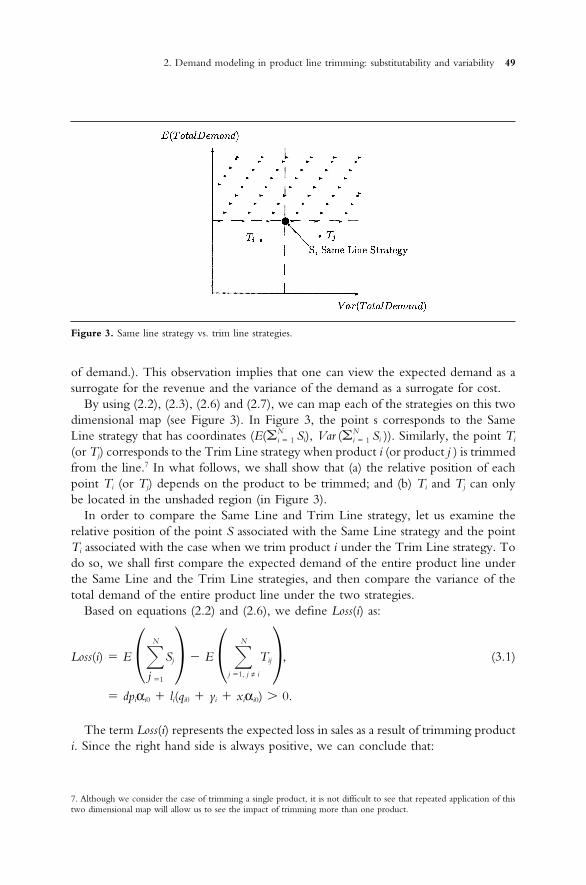
Figure 3. Same line strategy vs. trim line strategies.
of demand.). This observation implies that one can view the expected demand as asurrogate for the revenue and the variance of the demand as a surrogate for cost.
By using (2.2), (2.3), (2.6) and (2.7), we can map each of the strategies on this twodimensional map (see Figure 3). In Figure 3, the point s corresponds to the SameLine strategy that has coordinates (E(�N
i � 1 Si), Var (�Ni � 1 Si )). Similarly, the point Ti
(or Tj) corresponds to the Trim Line strategy when product i (or product j ) is trimmedfrom the line.7 In what follows, we shall show that (a) the relative position of eachpoint Ti (or Tj) depends on the product to be trimmed; and (b) Ti and Tj can onlybe located in the unshaded region (in Figure 3).
In order to compare the Same Line and Trim Line strategy, let us examine therelative position of the point S associated with the Same Line strategy and the pointTi associated with the case when we trim product i under the Trim Line strategy. Todo so, we shall first compare the expected demand of the entire product line underthe Same Line and the Trim Line strategies, and then compare the variance of thetotal demand of the entire product line under the two strategies.
Based on equations (2.2) and (2.6), we define Loss(i) as:
Loss(i) � E ��N
j �1
Sj� � E � �N
j �1, j ≠ i
Tij�, (3.1)
� dpiαi0 � li(qi0 � yi � xiαi0) � 0.
The term Loss(i) represents the expected loss in sales as a result of trimming producti. Since the right hand side is always positive, we can conclude that:
7. Although we consider the case of trimming a single product, it is not difficult to see that repeated application of thistwo dimensional map will allow us to see the impact of trimming more than one product.
50 I. New products and existing product portfolio management
Observation 1: The expected total demand associated with the Trim Line strategy isalways lower than that of the Same Line strategy.8
This observation implies that all points Ti will be located in the unshaded region inFigure 3; i.e., either at the south-west quadrant or the south-east quadrant from thepoint S. Note that the following remarks follow from (3.1):
• Loss(i) increases in dpi and li. Thus, products that have a smaller expected demand(i.e., dpi � li) tend to result in a smaller loss in the demand for the entire productline. This result may appear to support the ‘lame duck’ heuristic. However, theexpression for Loss(i) also suggests that the loss is mediated by other parameters.9
• Loss(i) increases in yi. Thus, highly unique products should not be trimmed becausethey are more likely to lead to customers leaving the product category, i.e., yi ishigh.
• Loss(i) increases in xi. In other words, products that exhibit significant ‘brand weak-ening’ phenomena, i.e. high probability of joining disloyal segment, should not betrimmed.
• Loss(i) increases in αi0 and/or qi0. It follows from the definitions of αi0 and qi0 thatαi0 and qi0 increase when the competitive product 0 is a better substitute for producti than that of other products belonging to the firm. To reduce the expected loss ofsales under the Trim Line strategy, it is desirable to trim a product i that has closesubstitutes offered by the firm but not offered by the competitors. This observationhighlights the significance of product substitutability when deciding the product tobe trimmed.
Next, based on equations (2.3) and (2.7), we define Reduction(i) as:
Reduction(i) � Var��N
j � 1
Sj � � Var � �N
j � 1, j ≠ i
Tij�,
� dp0(1 � p0) � {d (p0 � αi0pi)(1 � p0 � α i0pi)
� li(yi � qi0 � αi0xi) (1 � yi � qi0 � αi0xi)}, (3.2)� dαi0pi (2p0 � αi0pi � 1)
� li(yi � qi0 � αi0xi) (1 � yi � qi0 � αi0xi). (3.3)
The term Reduction(i) represents the reduction of variance in sales as a result of trim-ming product i. Notice from (3.3) that Reduction(i) can be either positive or negative.
8. Note that our model does not incorporate the possibility that a smaller number of products may lead to increased salesbecause of less customer confusion.9. Intuitively, dpi � li is the maximum potential loss and Loss(i) is the expected loss after accounting for consumer switchingbehaviors.

2. Demand modeling in product line trimming: substitutability and variability 51
This implies that the total variance can either decrease or increase as a result of trim-ming product i. In this case, we can conclude that:
Observation 2: Depending on the values of the parameters, the variance of the total demandassociated with the Trim Line strategy can be lower or higher than that of the Same Line strategy.
Based on (3.2), we can make the following remarks:
• When p0 � 0.5 and (p0 � αi0 pi) � 0.5, we have Reduction (i) � 0.10 That is, if thefirm holds a dominant position in the disloyal segment before line trimming (i.e.,�i � N
i � 1 pi � 1 � p0 � 0.5), trimming a product always lead to an increase in thevariance of the demand of the entire product line. This finding implies that a leaderin the disloyal segment is less likely to trim a product. Put differently, a dominantleader may have a wider product line than followers.
• When p0 � 0.5, and d �� li, we have Reduction (i) � 0. In words, if the firm hasless than 50% market share in a large disloyal segment, then the firm can reduce itsvariance of the demand for the entire product line by trimming the product line.
Similarly, the following remarks follow from (3.3):
• Reduction(i) increases in pi when p0 � 0.5. This implies that the larger the marketshare of a product in the disloyal segment where the competitor is a market leader,the more attractive (from the viewpoint of variance reduction) is trimming thatproduct to the firm.
• Reduction(i) increases in p0 . If the firm has low market share in the disloyal segment,then the firm can reduce its variance by trimming the product line.
• Reduction(i) decreases in qi0 if yi � qi0 � αi0xi � 0.5. So, if the trimmed product issimilar to any of competitive products, the firm can experience an increase in thevariance. This observation and the fact that Loss(i) increases in qi0 imply that trim-ming a product similar to any competitive product reduces the expected value andsimultaneously increases the variance of the demand for the entire product line.
• Reduction(i) decreases in li. If each product has a sufficiently large loyal segment,then Reduction(i) � 0 for all i; hence it does not pay to trim.
Based on observations 1 and 2, each point Ti would either located at the south-westquadrant or the south-east quadrant from the point S (see Figure 3). For any pointTi located at the south-east quadrant from the point S, there is a decrease in theexpected demand and an increase in the variance of the demand if the firm trimsproduct i from its product line. Clearly, it is undesirable to trim a product i whenthe corresponding point Ti is located at the south-east quadrant from the point S.This observation enables us to specify a necessary condition under which the same linestrategy is optimal as follows:
10. Note that x(1 � x) increases in x for x � 0.5 and decreases in x for x � 0.5.
52 I. New products and existing product portfolio management
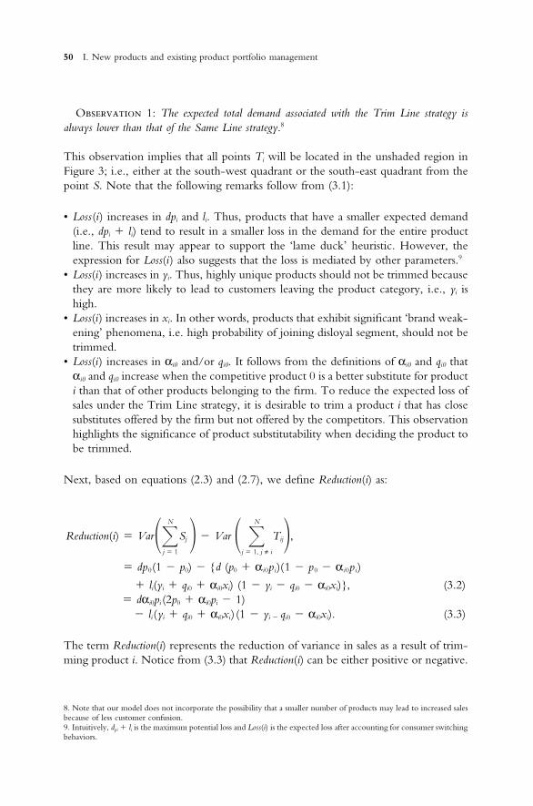
Figure 4. Optimality condition for same line strategy.
Observation 3: If Reduction(i) � 0 for each i, where i � 1, . . . , N, then the SameLine strategy is optimal.11
If all Ti, (i � 1, . . . , N), are located at the south-east quadrant, the Same Linestrategy is optimal (see Figure 4). When the above condition does not hold, thenthere exists a set of products, denoted by C, where
C � {i : Reduction(i) � 0, i � 1, . . . ,N} (3.4)
such that there will be a reduction in the variance of the demand as a result fromtrimming product i ∈ C from the line. In this case, for each product i in the set C,the corresponding point Ti will be located at the south-west quadrant as depicted inFigure 4. Even though there is a reduction in variance when we trim a product i ∈C, an expected loss, Loss(i), would result from trimming product i. Hence, it is neces-sary to evaluate the trade-off between expected loss in demand and the reduction inthe variance when selecting a product to trim. The actual trade-off would dependon the price/cost structure, which is beyond the scope of this paper.
In light of Observation 3, we now investigate the impact of substitutability, αij, onthe Same Line and Trim line strategies. Since �N
j � 0, j ≠ i αij � 1, we can express αi0,the substitutability of the competitive product for the firm’s product, as αi0 � 1 ��N
j � 1, j ≠ i αij. In this case, the substitutability with the competitive product, αi0, de-creases linearly as the substitutability with the firm’s remaining product line,�N
j � 1, j ≠ i αij increases. Hence, studying the impact of the substitutability with thecompetitive product, αi0, is equivalent to studying the impact of substitutability withthe firm’s remaining product line, �N
j � 1, j ≠ i αij. For this reason, it suffices to focus
11. We assume that all benefits derived from trimming the product line are captured by the variance term. This is areasonable assumption if the manufacturing technology is flexible enough that the unit cost is not affected by the numberof products in the product line.
2. Demand modeling in product line trimming: substitutability and variability 53
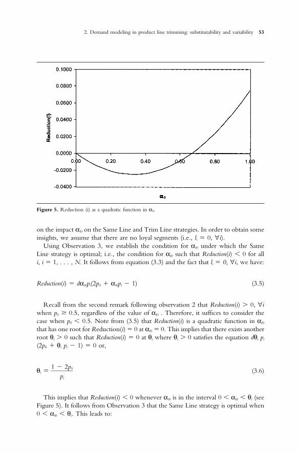
Figure 5. Reduction (i) as a quadratic function in α0.
on the impact αi0 on the Same Line and Trim Line strategies. In order to obtain someinsights, we assume that there are no loyal segments (i.e., li � 0, ∀i).
Using Observation 3, we establish the condition for αi0 under which the SameLine strategy is optimal; i.e., the condition for αi0 such that Reduction(i) � 0 for alli, i � 1, . . . , N. It follows from equation (3.3) and the fact that li � 0, ∀i, we have:
Reduction(i) � dαi0pi(2p0 � αi0pi � 1) (3.5)
Recall from the second remark following observation 2 that Reduction(i) � 0, ∀iwhen p0 � 0.5, regardless of the value of αi0 . Therefore, it suffices to consider thecase when p0 � 0.5. Note from (3.5) that Reduction(i) is a quadratic function in αi0
that has one root for Reduction(i) � 0 at αi0 � 0. This implies that there exists anotherroot θi � 0 such that Reduction(i) � 0 at θi where θi � 0 satisfies the equation dθi pi
(2p0 � θi pi � 1) � 0 or,
θi �1 � 2p0
pi
(3.6)
This implies that Reduction(i) � 0 whenever αi0 is in the interval 0 � αi0 � θi (seeFigure 5). It follows from Observation 3 that the Same Line strategy is optimal when0 � αi0 � θi. This leads to:
54 I. New products and existing product portfolio management
Observation 4: Consider a market consists entirely of disloyal segment (i.e., li � 0, ∀i).If the firm is a market leader in the disloyal segment (i.e., p0 � 0.5) and the substitutabilitiesof competitive product for the firm’s products are sufficiently low (i.e., when αi0 � θi , ∀i),then the Same Line strategy is optimal.
We now relate Observation 4 to the case in which product substitutability conformsto the classical attraction model of Bell, Keeney and Little (1975).12 First, it can beshown (see Appendix) that the substitutability αij relates to the market share of productj in the disloyal segment pj and the market share of the trimmed product i in thedisloyal segment pi as follows:
αij �pj
1 � p i
(3.7)
and correspondingly for αi0,
αi0 �p0
1 � pi
(3.8)
It follows from (3.6) and (3.8) that the condition αi0 � θi can be rearranged into:
1 � 2p0
p0
�pi
1 � pi
(3.9)
In this case, as stated in observation 4, Same Line strategy is optimal if (3.9) is truefor all i. In other words, Same Line strategy is optimal if
1 � 2p0
p0
� maxi
{pi
1 � pi
} (3.10)
Notice that condition (3.10) is more likely to hold when the term maxi {pi/(1 �pi)} is minimized. Suppose that p0 is fixed. Hence, �ip i � 1 � p0 is also fixed. In thiscase, it is easy to see that maxi {pi/(1 � pi)} is minimized when the pi’s are all equal.This implies that when the competitive market share p0 is fixed, the Same Line strategyis more likely to be optimal if the market shares of the firm’s products do not differvery much among themselves.
12. Assumption A4 of the classical attraction model by Bell, Keeney and Little (1975) assumes that the market share ofa seller depends on the magnitude of the change in the attraction of other seller(s) but does not depend on which seller(s)is making the change. In other words, the change in the attraction of a seller does not impact differentially on other sellers(i.e. no asymmetry). By construction, our model allows for such an asymmetry because no specific form of substitutability,αij, is assumed

2. Demand modeling in product line trimming: substitutability and variability 55
Figure 6. Lame duck strategy does not results in minimum loss.
4. THE LAME DUCK HEURISTIC
In the last section, we have presented a framework to analyze the conditions underwhich the Same Line strategy is optimal. In the event the same line strategy may notbe optimal, the framework has also suggested a potential set of candidates to betrimmed. Now, we apply our framework to analyze the effectiveness of a commonproduct trimming heuristic, i.e., the lame duck heuristic.13 Specifically, the lame duckheuristic prescribes the elimination of product k, where
k � argmin {j : E(Sj), j � 1, . . . , N} � argmin{j : lj � dpj, j � 1, . . ., N}. (4.1)
By (4.1), it is obvious that the lame duck heuristic ignores the demand interactionsand the substitutability among products.14 Without taking into account substitutability,the lame duck heuristic can be flawed for three reasons, as stated in the followingthree observations:
Observation 5: In general, trimming the lame duck will not result in minimum loss inexpected sales (i.e., k ≠ i* where i* � argmin { j : loss(j), j � 1, . . . , N}). However, ifli � 0, ∀i and the classical attraction model for market share holds for the disloyal segment,then k � i*.
In Figure 6, the point Tk corresponds the lame duck whereas the point Ti* corre-sponds to the product where trimming it results in minimum loss (or maximum ex-pected demand after trimming). This can happen when the lame duck is a closersubstitute to the competitive product than some products in the firm’s product line.
13. Various surveys in the literature cited in the introduction suggest that this is a common practice.14. Assumption A4 of the attraction model by Bell, Keeney and Little (1975) basically implies that the impact of trimmingis symmetric and linear. That is the impact of trimming product i on product j is proportionate to the market share ofproduct j , which implicitly ignores the differences in substitutability. By trimming the product with smallest market share,the attraction model predicts a minimum loss of market share; hence, the attraction model essentially prescribes a lameduck selection.
56 I. New products and existing product portfolio management
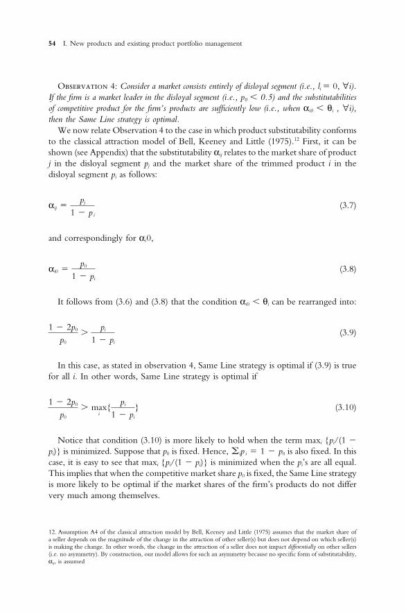
Figure 7. Lame duck strategy results in increased variance.
This can also happen when the lame duck is sufficiently unique that its removal resultsin a big portion of the loyal customers leaving the market.
Trimming lame duck will result in minimum loss when the attraction model isvalid. To elaborate, let us consider the case in which the loyal segments are empty.From (3.1), we have Loss(i) � dαi0pi. If the substitutability of competitive productfor product i, αi0, conforms to equation (3.8)(i.e., αi0 agrees with the attraction model),then we have:
Loss(i) � dp0
1 � pi
pi � dp0pi
1 � pi
,
which can be minimized by choosing the product with the smallest pi. Notice from(4.1) that the lame duck heuristic will select the product with the smallest pi. In thiscase, we can conclude that the lame duck heuristic will produce minimum loss whenthe attraction model is valid.
Observation 6: Under certain scenarios (discussed below), trimming the lame duck canresult in a loss in sales and a simultaneous increase in demand variability, i.e., Reduction(k) � 0 and loss(k) � 0. Thus, it is sub optimal.
Let us consider two cases. First, suppose that Reduction(i) � 0 for all i. Recall fromthe first remark following Observation 2 that this happens when the firm is a marketleader (i.e. p0 � 0.5) and each product does not have a significantly larger marketshare than others in the product line. In this case, Observation 3 implies that the SameLine strategy is optimal. Hence, the firm should not trim any product and the lameduck heuristic is definitely not appropriate. In the second case, suppose there existssome products j such that Reduction ( j ) � 0 for each j . Then the set C, as definedin (3.4), is not empty. Hence, it is quite reasonable to trim a product that belongs tothe set C such that there is a reduction in the variance of the demand as a result ofproduct trimming. Figure 7 depicts the case when C � {1,2,3} and k ∉ C. Since k
2. Demand modeling in product line trimming: substitutability and variability 57
Figure 8. Lame duck strategy is dominated by trim i strategy.
∉ C, trimming product k would increase the variance of the demand (in addition tosome loss in the expected sales, loss(k)). A possible scenario that could result in abovesituation is when the lame duck is sufficiently unique in the firm’s product line, trim-ming the product results in the loyal customers either leaving the market completely(i.e. yk �� 0) or joining the disloyal segment (i.e. xk �� 0).
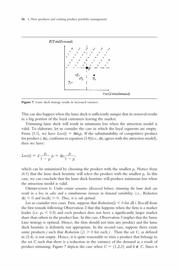
Observation 7: Under certain scenario (discussed below), trimming the lame duck can bedominated even if it belongs to the trim set (i.e., k ∈ C).
In other words, there exists at least one other product when trimmed is no worse offthan trimming the lame duck and is strictly preferred on at least one of the two dimen-sions, i.e. expected demand and variance of demand. Figure 8 depicts such a case.In Figure 8, the point Tk corresponds the lame duck whereas the point Ti, locatednorth-west from Tk, corresponds to a product when trimmed results in smaller loss andlarger variance reduction than trimming the lame duck. One scenario where thelame duck is dominated is when the lame duck is highly substitutable by the com-petitive product in a market where the competitor has major market share in the disloyalsegment.
5. AN ILLUSTRATIVE EXAMPLE
This section presents a numerical example that intends to serve two purposes: (1) toillustrate our findings in previous sections and (2) to show that lame duck heuristiccan be flawed.
Consider a firm that offers two products, 1 and 2. Each product has a moderatesize of loyal segment (l1 � 10,l2 � 20). The disloyal segment is large compared tothe loyal segments (d � 400). Within the disloyal segment, the competitor is themarket leader and product 1 has a larger market share than product 2. In our example,we have p0 � 0.7, p1 � 0.2 and p2 � 0.1.
Based on managerial subjective estimates, the parameters associated with trimmingproduct i are the same for both products 1 and 2. Specifically, upon trimming product
58 I. New products and existing product portfolio management
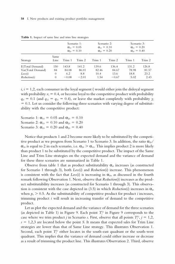
Table 1. Impact of same line and trim line strategies
Scenario 1: Scenario 2: Scenario 3:α10 � 0.05 α10 � 0.10 α10 � 0.20α20 � 0.10 α20 � 0.20 α20 � 0.40
SameStrategy Line Trim 1 Trim 2 Trim 1 Trim 2 Trim 1 Trim 2
E(Total Demand) 150 143.8 141.2 139.6 136.4 131.2 126.8Var(Total Demand) 84 84.08 86.01 82.46 84.67 78.98 81.57Loss(i) 0 6.2 8.8 10.4 13.6 18.8 23.2Reduction(i) 0 �0.08 �2.01 1.54 �0.67 5.02 2.43
i, i � 1,2, each consumer in the loyal segment li would either join the disloyal segmentwith probability xi � 0.4, or become loyal to the competitive product with probabilityqi0 � 0.1 (and q12 � q21 � 0.4), or leave the market completely with probability yi
� 0.1. Let us consider the following three scenarios with varying degree of substitut-ability with the competitive product:
Scenario 1: α10 � 0.05 and α20 � 0.10Scenario 2: α10 � 0.10 and α20 � 0.20Scenario 3: α10 � 0.20 and α20 � 0.40
Notice that products 1 and 2 become more likely to be substituted by the competi-tive product as we progress from Scenario 1 to Scenario 3. In addition, the ratio α20/α10 is equal to 2 in each scenario, i.e. α20 � α10. This implies product 2 is more likelythan product 1 to be substituted by the competitive product. The impact of the SameLine and Trim Line strategies on the expected demand and the variance of demandfor these three scenarios are summarized in Table 1.
Observe from table 1 that as product substitutability αi0 increases (as constructedfor Scenario 1 through 3), both Loss(i) and Reduction(i) increase. This phenomenonis consistent with the fact that Loss(i) is increasing in αi0, as discussed in the fourthremark following Observation 1. Next, observe that Reduction(i) increases as the prod-uct substitutability increases (as constructed for Scenario 1 through 3). This observa-tion is consistent with the case depicted in (3.5) in which Reduction(i) increases in αi0
when p0 � 0.5. As the substitutability of competitive product for product i increases,trimming product i will result in increasing transfer of demand to the competitiveproduct.
Let us plot the expected demand and the variance of demand for the three scenarios(as depicted in Table 1) in Figure 9. Each point T(s)
j in Figure 9 corresponds to thecase where we trim product j in Scenario s. First, observe that all points T(s)
j , j � 1,2,s � 1,2,3 are located below the point S. It means that expected sales for Trim Linestrategies are lower than that of Same Line strategy. This illustrates Observation 1.Second, each point T(s)
j either locates in the south-east quadrant or the south-westquadrant. This implies that the variance of demand could either increase or decreaseas a result of trimming the product line. This illustrates Observation 2. Third, observe
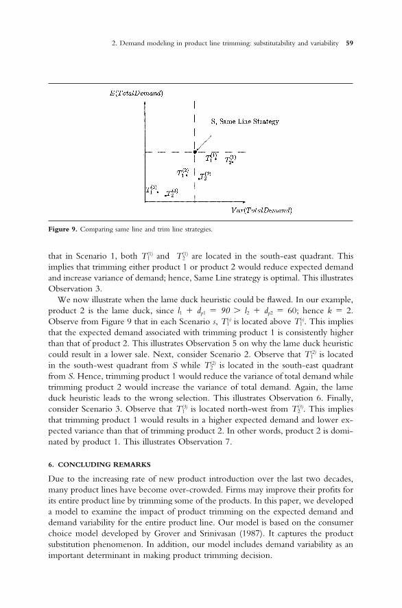
2. Demand modeling in product line trimming: substitutability and variability 59
Figure 9. Comparing same line and trim line strategies.
that in Scenario 1, both T(1)1 and T(1)
2 are located in the south-east quadrant. Thisimplies that trimming either product 1 or product 2 would reduce expected demandand increase variance of demand; hence, Same Line strategy is optimal. This illustratesObservation 3.
We now illustrate when the lame duck heuristic could be flawed. In our example,product 2 is the lame duck, since l1 � dp1 � 90 � l2 � dp2 � 60; hence k � 2.Observe from Figure 9 that in each Scenario s, T(s)
1 is located above T(s)1 . This implies
that the expected demand associated with trimming product 1 is consistently higherthan that of product 2. This illustrates Observation 5 on why the lame duck heuristiccould result in a lower sale. Next, consider Scenario 2. Observe that T(2)
1 is locatedin the south-west quadrant from S while T(2)
2 is located in the south-east quadrantfrom S. Hence, trimming product 1 would reduce the variance of total demand whiletrimming product 2 would increase the variance of total demand. Again, the lameduck heuristic leads to the wrong selection. This illustrates Observation 6. Finally,consider Scenario 3. Observe that T(3)
1 is located north-west from T(3)2 . This implies
that trimming product 1 would results in a higher expected demand and lower ex-pected variance than that of trimming product 2. In other words, product 2 is domi-nated by product 1. This illustrates Observation 7.
6. CONCLUDING REMARKS
Due to the increasing rate of new product introduction over the last two decades,many product lines have become over-crowded. Firms may improve their profits forits entire product line by trimming some of the products. In this paper, we developeda model to examine the impact of product trimming on the expected demand anddemand variability for the entire product line. Our model is based on the consumerchoice model developed by Grover and Srinivasan (1987). It captures the productsubstitution phenomenon. In addition, our model includes demand variability as animportant determinant in making product trimming decision.
60 I. New products and existing product portfolio management
Our model exhibits the common observation that product line trimming leads toincreased individual demands but to a reduced demand for the entire product line.Contrary to conventional wisdom, our model suggests that trimming the productwith the minimal expected demand (i.e. the lame duck heuristic) can be flawed. Weshowed that this heuristic is deficient in three respects. First, it may not lead to minimalrevenue loss. Second, even if it leads to minimal revenue loss, it can be sub-optimalif it leads to an increase in variance. Third, the lame duck heuristic may be dominated.Trimming another product may yield a lower loss and a higher variance reduction inexpected demand. The heuristic appears to work well only when there is no demandsubstitution among products.
Carrying a smaller product line may not be strategically desirable for some firms.Smaller product line may translate to reduced presence at the retail front. Considerthe grocery industry. Due to limited shelf space, supermarkets often allocate a fixedshelf space for carrying and displaying products from a particular manufacturer. Thus,the manufacturer may have to keep the breath of product line fixed to justify theshelf space. Consequently, the firm must determine which product to eliminate andwhich one to introduce. This product replacement decision is like a ‘football-team’problem in which the ‘coach’ has to configure the best team to compete in the field.
Chong, Ho and Tang (2001) proposed a framework to capture the effect of productreplacement on sales. Since their model conforms to the classical attraction model ofBell, Keeney and Little (1975), product substitutability implied by their model is simi-lar to equation (3.7). Furthermore, they did not use sales variance in their modelingframework. By hybridizing our model with that of Ho and Tang (1995)15, we canhave a model setup more general than Chong, Ho and Tang (2001). This generalhybridized model seems like a logical next step for this research.
APPENDIX A: PROOF OF EQUATION (3.8)
By the definition of market share from Bell, Keeney and Little (1975), we have,
pj �Aj
�Nl � 0 Al
, ∀j ,
where Al is the level of attraction of product l, as defined in Bell, Keeney and Little(1975). If product i is trimmed, we have the corresponding revised market share:
pj � αijpi �Aj
�Nl � 0,l ≠ i Alc,
∀j,
From the two equations above, we have,
15. The authors examined the issue of product line extension. The paper suggested conditions under which line extensionis beneficial and related the benefits of line extension to market leadership and manufacturing capability.
2. Demand modeling in product line trimming: substitutability and variability 61
αij � � Aj
�Nl � 0,l ≠ iAl
�Aj
�Nl � 0Al
� /Ai
�Nl � 0Al
,
�Aj
Ai
� �Nl � 0 Al
�Nl � 0,l ≠ iAl,
� 1�,
�Aj
Ai
� 1 �Aj
�Nl � 0,l ≠ iAl
� 1 �,
�Aj
�Nl � 0,l ≠ iAl
,
� pj � αijpi.
This implies that,
αij �pj
1 � pi
and also,
αi0 � 1 � �N
j � 1, j ≠ i
αij,
� 1 � �N
j � 1, j ≠ i
pj
1 � pi
,
�p0
1 � pi
.
REFERENCES
1. Alexander, Ralph S., ‘The Death and Burial of Sick Products,’Journal of Marketing, Vol 28, (April 1964),pp. 1–7.
2. Avlonitis, G.J., ‘Production Elimination Decision Making: Does Formality Matter?’ Journal of Marketing,Vol. 49, (Winter 1985), pp. 41–52.
3. Avlonitis, G.J. and James, B.G.S., ‘Some Dangerous Axioms of Product Elimination Decision-Making,’European Journal of Marketing, Vol. 16, No. 1 (1982), pp. 36–48.
4. Bell, D., Keeney, R. and Little, J., ‘A market share theorem,’ Journal of Marketing Research, Vol. 12(August 1975), pp. 136–141.
5. Berenson, Conrad, ‘Pruning the Product-Line,’ Business Horizons, Vol 6, (Summer 1963), pp. 63–70.6. Browne, W.G. and Kemp, P.S., ‘A Three Stage Product Review Process,’ Industrial Marketing Manage-
ment, 5, (Dec 1976), pp. 333–342.7. Bayus, B. and Putsis, W., ‘Product Proliferation: An Empirical Analysis of Product Line Determinants
and Market Outcomes,’ Marketing Science, Vol. 18, No. 2, (1999), pp. 137–153.8. Chong, J.K., Ho, T.H. and Tang, C.S., ‘A Modeling Framework for Category Assortment Planning,’
Manufacturing & Service Operations Management, Vol. 3, No. 3, (2001), pp. 191–210.9. Corstjens, M. and Weinstein, D., ‘Optimal Strategic Business Units Portfolio Analysis,’ TIMS Studies
in the Management Sciences, 18, (1982), pp. 141–160.10. Green, Paul E. and Krieger, Abba M., ‘Conjoint Analysis with Product Positioning Applications,’ in
62 I. New products and existing product portfolio management
J. Eliashberg and G.L. Lilien, Eds., Handbooks in Operations Research and Management Science, Vol 5:Marketing, North-Holland, Amsterdam, (1993), pp. 467–515.
11. Greenley, G., and Bayus, B., ‘A Comparative Study of Product Launch and Elimination Decision inUK and US companies,’ European Journal of Marketing, vol. 28, (1994), pp. 5–29.
12. Grover, R. and Srinivasan, V., ‘A Simultaneous Approach to Market Segmentation and Market Struc-turing,’ Journal Of Marketing Research, Vol. 24 (may 1987), pp. 139–153.
13. Hamelman P.W. and Mazze, E.M., ‘Improving Product Abandonment Decisions,’ Journal Of Marketing,Vol. 36, (April 1972), pp. 20–26.
14. Hart, Susan J., ‘The Causes of Product Deletion in British Manufacturing Companies,’ Journal of Market-ing Management, Vol. 3 No. 3, (1988), pp. 328–343.
15. Hays, L., ‘Too Many Computer Names Confuse Too Many Buyers,’ Wall Street Journal, (June 29,1994), B1, B6.
16. Hise, R.T. and McGinnis, M.A., ‘Product Elimination: Practices, Policies, and Ethics,’ Business Hori-zons, 18, (June 1975), pp. 25–32.
17. Hise, R.T., Parasuraman, A. and Viswanathan, R., ‘Product Elimination: The Neglected ManagementResponsibility,’ The Journal of Business Strategy, Vol. 4, No. 4, (Spring 1984), pp. 56–63.
18. Ho, T and Tang, C.S., ‘When is Product Line Extension Beneficial?’ UCLA Working Paper, (1995)19. Khermouch, G., ‘Amid Rampant Product Proliferation, Beverage Marketers Desperately Seeking Sim-
plicity,’ Brandweek, (May 29, 1995), 1, 9.20. Kotler, P., ‘Phasing-out Weak Products,’ Harvard Business Review, Vol. 43, (March-April, 1965), pp.
108–118.21. Larreche, J.C. and Srinivasan, V., ‘STRATPORT: A Model for the Evaluation and Formulation of
Business Portfolio Strategies,’ Management Science, Vol. 28, (1982), pp. 979–1001.22. Mahajan, V. and Wind, Y., ‘Integrating Financial Portfolio Analyses with Product Portfolio Models,’
in H. Thomas and D. Garner, Eds., Strategic Marketing and Management, John Wiley & Sons, (1985),pp. 193–212.
23. Mahajan, V., Wind, Y. and Bradford, J.W., ‘Stochastic Dominance Rules for Product Portfolio Analy-sis,’ TIMS Studies in the Management Sciences, 18, (1982), pp. 161–183.
24. Narisetti, R., ‘P&G, Seeing Shoppers Were Being Confused, Overhauls Marketing,’ Wall Street Journal,(January 15, 1997), A1, A8.
25. Putsis, W. and Bayus, B., ‘An Empirical Analysis of Firms’ Product Line Decisions,’ Journal of MarketingResearch, Vol. 38 (February 2001), pp. 110–118.
26. Quelch, J. and Kenny, D., ‘Extend Profits, Not the Product Lines,’ Harvard Business Review, Vol. 72,(Sep–Oct, 1994), pp. 153–160.
27. Silver, E.A. and Peterson, R., Decision Systems for Inventory Management and Production Planning. JohnWiley & Sons, (1985).
28. Teinowitz, Ira and Lawrence, Jennifer, ‘Brand Proliferation Attacked,’ Advertising Age,1, (May 10 1993),pp. 49.
29. Urban, G.L., ‘A Mathematical Modeling Approach to Product Line Decisions,’ Journal of MarketingResearch,Vol. 6, (Feb. 1969), pp. 40–47.