Embed Size (px)
Citation preview

ESCUELA TÉCNICA SUPERIOR DE INGENIERÍA (ICAI)
INSTITUTO DE INVESTIGACIÓN TECNOLÓGICA
Proyecto Fin de Carrera
Modeling time-dependent demand elasticity in a Probabilistic Production Costing model
Application to the Spanish electricity market
Mikel Ayala Bernaola
Advisors: Carlos Batlle & Pablo Rodilla (IIT)
Madrid, May 25, 2011


Modeling demand elasticity in a Probabilistic Production Costing model. Application to the Spanish electricity market Proyecto Fin de Carrera – Mikel Ayala Bernaola
i
Table of Contents
1. INTRODUCTION, MOTIVATION & OBJECTIVES ........................................................... 1
1.1 Security of Generation Supply ................................................................................. 1
1.1.1 The 4 Dimensions of the Security of Supply Problem ...................................... 1
1.2 The Need for Regulatory Tools & Support Models .................................................... 2
1.3 The New Active Role of Demand ............................................................................. 3
1.3.1 Reliability Measures in the Presence of Demand Elasticity ............................... 3
1.4 PPC Models as a Tool to Assess System Performance................................................ 3
1.5 Scope and Objectives .............................................................................................. 4
1.6 Organization of this Document ................................................................................ 5
1.7 References .............................................................................................................. 5
2. A PROBABILISTIC PRODUCTION COSTING MODEL TO ESTIMATE THE RELIABILITY OF A POWER GENERATION SYSTEM ........................................................ 6
2.1 Introduction ............................................................................................................ 6
2.1.1 Structure of the Chapter .................................................................................. 6
2.2 Introduction to Probabilistic Production Costing Models .......................................... 6
2.3 The Conventional Thermal System Model ................................................................ 7
2.3.1 Modeling Assumptions ................................................................................... 7
2.3.2 The Loading Algorithm ................................................................................. 10
2.3.3 Basic Results Provided .................................................................................. 17
2.4 The Hydro-Thermal System Model ......................................................................... 18
2.4.1 Hydro Units Modelling ................................................................................. 19
2.4.2 Loading of Energy-Limited Units ................................................................... 20
2.4.3 Validity of the Expected Energy Convolution Model ...................................... 23
2.5 Introducing Renewable Generation in the Model ................................................... 25
2.6 Introducing Demand Elasticity in the Model ........................................................... 26
2.6.1 Modeling Price-Sensitive Demand ................................................................ 26
2.6.2 .Modeling Reserve-Sensitive Demand ........................................................... 29
2.7 Measuring the Value of Non-Purchased Energy ...................................................... 30
2.7.1 The Background of the Concept .................................................................... 30
2.7.2 Brief Overview of the VNPE Concept ............................................................ 30
2.7.3 Computation Model Description ................................................................... 31
2.8 Conclusions .......................................................................................................... 36
2.9 References ............................................................................................................ 36
ii
3. ADDRESSING THE TIME-DEPENDENT NATURE OF DEMAND ELASTICITY IN AN ELECTRICITY MARKET ................................................................................................. 39
3.1 Introduction .......................................................................................................... 39
3.1.1 Structure of the Chapter ................................................................................ 39
3.2 Basic Concepts ...................................................................................................... 39
3.3 The Neural-Gas ..................................................................................................... 40
3.4 Analysis of the Time-Dependent Demand Elasticity ................................................ 42
3.4.1 Determination of the Optimal Number of Clusters ........................................ 43
3.4.2 Division of the Time Scope of Analysis ......................................................... 46
3.4.3 Elastic Demand Clustering Tool .................................................................... 49
3.5 Conclusions .......................................................................................................... 50
3.6 References ............................................................................................................ 50
4. CASE EXAMPLE: APPLICATION TO THE SPANISH ELECTRICITY MARKET ................... 51
4.1 Introduction .......................................................................................................... 51
4.1.1 Structure of the Chapter ................................................................................ 51
4.2 The Spanish Electricity System ............................................................................... 51
4.2.1 Load Scenario .............................................................................................. 51
4.2.2 Thermal Generation ..................................................................................... 52
4.2.3 Hydro Generation ........................................................................................ 54
4.2.4 RES Generation ............................................................................................ 55
4.2.5 Elastic Demand ............................................................................................ 55
4.3 Simulation Structure .............................................................................................. 60
4.4 Case Example Results ............................................................................................ 62
4.4.1 Classical Reliability Measures ....................................................................... 64
4.4.2 Value of Non-Purchased Energy ................................................................... 64
4.5 Conclusions .......................................................................................................... 65
4.6 References ............................................................................................................ 66
5. CONCLUSIONS ........................................................................................................... 68
5.1 Summary ............................................................................................................... 68

Modeling demand elasticity in a Probabilistic Production Costing model. Application to the Spanish electricity market Proyecto Fin de Carrera – Mikel Ayala Bernaola
1
1. INTRODUCTION, MOTIVATION & OBJECTIVES
The energy industry, and in particular the electricity sector, has been subject to major reforms over the recent decades. Until these processes started, the activity that we now call generation supply was part of the chain of activities of vertically integrated utilities and was thus performed as either a public service or as a regulated monopoly.
Although these reforms have taken very different forms, all of them have shared a common approach that consists of taking steps towards introducing competition at any of the activities in which it was considered feasible. These reforms have been traditionally designated as “liberalization” or “deregulation” processes.
From the regulatory perspective, the fact is that in the case of the energy industry, the reform has entailed exactly the opposite. Rather than a “deregulatory” process, the industry has experienced an intensely “re-regulatory” one, see Borenstein & Bushnell (2000) or Ruff (2003).
In that context, the objective of regulation is, broadly speaking, to prevent from occurring inefficient outcomes that would otherwise occur (or inversely, to produce efficient outcomes that would otherwise not occur). In particular, the regulator must guarantee a minimum required level of security of supply.
1.1 Security of Generation Supply
Modern society depends critically on the availability of electricity. It is widely recognised that the lack of supply has dramatic social, economic and political consequences. Hence, avoiding emergency situations and ensuring that electric energy is supplied according to the desired quality standards represents a chief concern for regulators worldwide.
With the advance of electricity markets, regulation is increasingly required in order to supervise that the market is able to guarantee an adequate level of security of supply. This is particularly relevant at the generation activity, where the liberalization process has been far more intense.
1.1.1 The 4 Dimensions of the Security of Supply Problem
The problem of security of supply at the generation level can be split up into four major dimensions according to their time horizon (Rodilla, 2010). This classification not only facilitates a better understanding of the problem but also the design of the regulatory mechanisms if required. The four dimensions are the following:
• Security: the very short-term dimension. Defined by the North American Electric Reliability Council as the “ability of the electrical system to support unexpected disturbances such as electrical short circuits or unexpected loss of components of the system” (NERC, 1997).
• Firmness: the short to medium-term dimension. Defined in Batlle & Pérez-Arriaga (2008) as the ability of the already installed facilities to supply electricity efficiently.
2
This dimension is determined by the characteristics of the existing generation portfolio and the medium-term resource-management carried out by generators (fuel provision, water reservoir management, maintenance scheduling, etc.).
• Adequacy: the long-term dimension. Defined as the existence of enough available generation capacity (installed or expected to be installed) to efficiently meet demand in the long term.
• Strategic expansion policy, which concerns the very long-term availability of energy resources and infrastructures. This dimension usually entails the diversification of primary sources of energy through a balanced generation portfolio.
Figure 1.1-I The 4 dimensions of security of supply
1.2 The Need for Regulatory Tools & Support Models
Rodilla (2010) showed that in the “deregulated” and “liberalized” scheme that governs electricity business, the intervention of the regulator is vital to ensure that an appropriate level of security of supply is achieved.
This regulatory intervention, which is carried out in order to drive the market towards an efficient outcome, is in practice implemented by introducing additional mechanisms, that is to say, additional rules. These mechanisms are regulatory tools aimed at providing additional (and optimal) signals to market agents.
In order to perform this role adequately, the regulator needs another kind of tools: Assessment tools (models of different nature) that can be used either to evaluate the market performance and thus detect the need of introducing additional mechanisms, or to assist in the design of these mechanisms, by evaluating ex-ante the impact of the regulatory solutions that could be considered.
Modeling demand elasticity in a Probabilistic Production Costing model. Application to the Spanish electricity market Proyecto Fin de Carrera – Mikel Ayala Bernaola
3
1.3 The New Active Role of Demand
The active participation of the demand side in power systems has always been considered an important requirement for their well-functioning, particularly for that of the liberalized ones. Nonetheless, it has not played this desired key role so far due to several reasons (demand immaturity and lack of technical solutions).
This situation is highly expected to change in the near future with the upcoming technical and regulatory developments of smart-grids and demand response tools. In this new context, the ability to properly consider this new active role of demand into electric power system analysis tools turns to be essential.
1.3.1 Reliability Measures in the Presence of Demand Elasticity
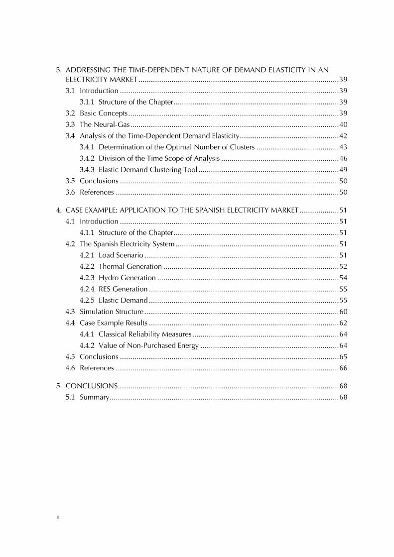
As highlighted by Rodilla & Batlle (2010), classical reliability measures such as the Loss Of Load Probability (LOLP), and the Expected Non-Served Energy (ENSE) leave aside very meaningful information when used to assess the performance of a system where elastic demand plays a significant role. As a matter of fact and as it can be checked in Figure 1.3.1-I, in a fully elastic demand scenario, the values of the LOLP and of the ENSE are, according to their traditional definition, always equal to zero. Consequently, even a permanent scenario of severe scarcity could be obscured by the use of the aforementioned metrics.
Figure 1.3.1-I Reliability measures in the presence of demand elasticity
In order to reflect the elastic consumption in the performance measure, the evaluation of the distribution function of what was termed as the Value of the Non-Purchased Energy (VNPE) was proposed.
1.4 PPC Models as a Tool to Assess System Performance
One of the tools that has been intensively used to support electric power systems long-term planning and reliability analysis are Probabilistic Production Costing models (PPC models).

4
These models have traditionally been used in electric power systems as a support tool in the centralized long-term decision-making process.
This approach has attracted considerable efforts from academia since the late 60’s. However, although some approaches have been developed to model load shifting programs, as for example Malik (2001), the literature has lacked until recently of efficient algorithms to explicitly introduce demand response to prices in PPC models.
In Rodilla & Batlle (2010) an algorithm that allows extending the classic PPC models design to explicitly represent demand elasticity was proposed.
1.5 Scope and Objectives
This dissertation addresses the problem of developing an adequacy analysis model for electricity markets in which elastic demand plays a significant role.
Taking as a starting point the PPC model approach proposed in Rodilla & Batlle (2010), we will formulate a PPC model to carry out reliability assessments of power generation systems where elastic consumption is substantial. The model proposed will be aimed at coping with a variety of peculiarities of electricity wholesale markets.
In addition to that or, we will face the challenge of developing a methodology that captures the time-dependent nature of elastic demand. The tool developed must allow for finding patterns and realistically describe the elastic demand of a given electricity market.
Eventually we will prove the capabilities of the model by analyzing a real-size case example based on the Spanish electricity market.
To summarize, the objectives of the dissertation are the following:
I. Develop a Probabilistic Production Costing model to estimate the adequacy of a power generation system. The following modelling challenges will have to be met.
I.A. Develop model that allows for analysis in a conventional thermal generation system with fully inelastic load.
I.B. Adapt the conventional PPC model for loading energy limited units.
I.C. Extend the PPC model with regard to taking into account intermittent renewable generation.
I.D. Construct an equivalent load and generation model to integrate price sensitive demand into the conventional PPC model as in Rodilla & Batlle (2010).
I.E. Adjust the PPC model in order to properly reflect the effect of the interruptible load described in MITyC (2007).
I.F. Develop an algorithm to compute the distribution function of the Value of the Non-Purchased Energy within the PPC frame-work.
Modeling demand elasticity in a Probabilistic Production Costing model. Application to the Spanish electricity market Proyecto Fin de Carrera – Mikel Ayala Bernaola
5
II. Address the time-dependent nature of demand elasticity in an electricity market. In order to do so, a robust and flexible clustering tool will be developed.
III. Carry out a simulation of the Spanish electricity market for 2016.
1.6 Organization of this Document
The document proceeds as follows. Chapter 2 describes the Probabilistic Production Costing model developed. In Chapter 3, a methodology to characterize the elastic demand of any given electricity market is formulated. Chapter 4 is devoted to the analysis of a real-size electricity market. Chapter 5 concludes and summarizes the results obtained.
1.7 References
Borenstein, S. & J. Bushnell (2000). “Electricity restructuring: Deregulation or reregulation. Regulation”. The Cato Review of Business and Government 23(2), pp.46-52, 2000.
Batlle, C. & I.J. Pérez-Arriaga (2008). “Design criteria for implementing a capacity mechanism in deregulated electricity markets”. Utilities Policy, 16(3):184-193, 2008.
Malik, A. S. (2001). “Modelling and Economic Analysis of DSM Programs in Generation Planning”, International Journal of Electrical Power & Energy Systems, Volume 23, Issue 5, June 2001.
MITyC, (2007). Ministerio de Industria y Comercio, Orden ITC/2370/2007, July 2007.
NERC (1997). “NERC Planning Standards”. North American Electric Reliability Council, September 1997.
Rodilla, P., Baíllo, A., Cerisola, S. & C. Batlle (2010). “Regulatory Intervention to Ensure an Efficient Medium-Term Planning in Electricity Markets”. Working Paper IIT-10-008A, submitted to Energy Economics.
Rodilla, P. (2010). “Regulatory Tools to Enhance Security of Supply at the Generation Level in Electricity Markets”. PhD Thesis. IIT, Universidad Pontificia Comillas, September 2010.
Rodilla, P. & C. Batlle (2010). “Redesigning Probabilistic Production Costing Models and Reliability Measures in the Presence of Market Demand Elasticity”. IIT Working Paper IIT-10- 028A, June 2010. Submitted to IEEE Transactions on Power Systems. Available at www.iit.upcomillas.es/batlle.
Ruff, L. E. (2003). “UnReDeregulating Electricity: Hard Times for a True Believer. Seminar on New Directions in Regulation”. Kennedy School of Government, Harvard University, Cambridge, MA, May 2003.
6
2. A PROBABILISTIC PRODUCTION COSTING MODEL TO ESTIMATE THE RELIABILITY OF A POWER GENERATION SYSTEM
2.1 Introduction
After having introduced, in Chapter 1, the general problem of Security-of-Supply at the generation level and, more specifically, the upcoming problem of appraising the reliability of a power system in a context where demand plays an increasingly active role; we proceed now to introduce the model which constitutes the main theme of the present study.
This chapter can be considered to be the conceptual core of this dissertation. It describes in detail the formulation proposed to carry out reliability assessments of power generation systems in electricity markets where elastic demand consumption is substantial. The model design is aimed towards being a valid tool to cope with a variety of peculiarities of electricity wholesale markets.
2.1.1 Structure of the Chapter
The Chapter proceeds as follows. Section 2.2 reviews the concept of Probabilistic Production Costing model and the relevant literature. Then, in Section2.3, we describe the conventional thermal model, its assumptions, the dispatching algorithm and the results provided. Next, in Section 2.4, we explain how energy-limited units (typically hydro units) can be modelled, how their dispatch can be carried out and discuss some of its implications concerning reliability assessments. In Section 2.5 we show how intermittent renewable generation can be included in the model. In Section 2.6 we show how elastic demand can be modeled within the Probabilistic Production Costing model methodology. In Section 2.7 we provide a general formulation of the VNPE calculation algorithm. Section 2.8 concludes and discusses some applications and extensions.
2.2 Introduction to Probabilistic Production Costing Models
As described in Rodilla (2010), Probabilistic Production Costing models (in the following PPC models) have traditionally been used as a support tool in electric power systems, where they are particularly applicable to the centralized long-term decision-making process. These models are characterized by being focused in representing the random nature of some of the most relevant variables involved in the long-term planning problem (typically the demand values and the available capacity of each generating unit).
This approach allows for reliability assessments of real-size electric power systems with little computational effort. However, achieving that requires making severe simplifications regarding mainly short and medium-term operational and planning constraints of the generation plants.
The PPC framework has attracted considerable efforts from academia since the late 60’s. The basic model was applied to a non-constrained thermal system; see the pioneering works of Baleriaux et al. (1967) and Booth (1972).
Modeling demand elasticity in a Probabilistic Production Costing model. Application to the Spanish electricity market Proyecto Fin de Carrera – Mikel Ayala Bernaola
7
The major outputs that were first calculated by means of these models were:
• Reliability measures: the loss of load probability (LOLP), the loss of load expectancy (LOLE) and the expected value of the non-served energy (ENSE) among others.
• Expected production schedules, that is, the expected energy generated by each generating unit (in average).
• Expected production costs (idem).
It is important to note that there are a considerable number of papers addressing several variations on the conventional approach. For instance, there are remarkable works focused on introducing simplified alternatives to include either hydraulic units as in Finger (1979), Ramos et al. (1991) or Malik (2004); storage units as in Conejo (1987) or Invernizzi et al. (1988); or time-dependent units as in Conejo et al. (1985).
One of the most popular extensions to the basic model is the so-called frequency and duration method. This extension takes into account information on both the frequency and the duration of the different states (demand interval, outage rates, etc), and allows calculating additional results as, for example, the mean time existing between two consecutive critical events (most typically scarcities). This frequency and duration methodology embraces a whole set of different approaches. See for instance the works of Halperin & Adler (1958), Ringlee & Wood (1969), Ayoub & Patton (1976) or Finger (1979).
Additional relevant research has been conducted within the PPC framework, for example in Leite da Silva et al. (1988) or in Lee et al. (1990) a means to calculate the underlying variance of the results is provided. A description on how to estimate derivatives (e.g. marginal values), can be found in Ramos et al. (1994) and also in Maceira & Pereira (1996).
These PPC models have been extensively applied to determine the marginal contribution of each generating unit to the regulator’s reliability objectives. One of the first works on this topic is the one carried out by Garver (1966). A more recent work that addresses the problem of determining this contribution to reliability objectives (in this particular case, the contribution of wind energy) applying a PPC model can be found in Kahn (2004). This sort of calculations have been used, for example, to set the compensation for each generating unit in some real systems in which a capacity payment mechanism had been implemented (this was the case of the former Chilean mechanism or the Panamanian case among others).
2.3 The Conventional Thermal System Model
In this section, we describe the conventional thermal model, its underlying assumptions, the dispatching algorithm (which is, in fact, the core of the model) and the basic results it provides.
2.3.1 Modeling Assumptions
The simplest conventional PPC model is built upon two central assumptions. On the one hand, it is assumed that all generation plants can produce at full capacity at any time unless

8
when they are out-of-order due to a forced outage. On the other hand, hourly load is considered to be inelastic and stochastic.
These models were conceived to check a fairly simple reliability condition: whenever the system’s inelastic demand exceeds the available generating capacity a loss of load takes place. The probability of such an event happening (the Loss of Load Probability or LOLP) and the corresponding expected value of the non-served energy (ENSE), have been the most noteworthy results obtained from these models regarding reliability.
In such a context, the loss of load probability distribution can be evaluated by means of the distribution of the difference between two random variables: the demand and the total generation available. This difference is usually evaluated in a generic random hour. Longer term results (e.g. the expected non-served energy in a whole year) can be calculated by directly extending the results obtained when computing this generic hour.
If all variables (demand and available generation capacity in the most simple case) are statistically independent, then the computation of the former difference considerably simplifies, since the sum (or difference) of two independent random variables is equal to the convolution of their probability distribution functions.
We next present how the demand and the thermal generating units are modeled and the order followed in the convolution operation to simulate the generating units’ scheduling. Then we explain how to interpret the results obtained when performing this operation.
The Demand Curve
The empirical (de-cumulative) distribution function of the load is commonly accepted as a well suited proxy for the distribution function of the electricity demand in a generic random hour.
The empirical de-cumulative distribution function of the Load, or empirical DDF, is the DDF associated with the empirical measure of a sample of observations (i.e. a set of k hourly
load values): It is usually denoted by )(ˆ LSk and estimates the true underlying DDF of the
sampled hourly load, referred to as )(LS . More formally, the estimator )(ˆ LSk is said to
converge almost surely to )(LS as ∞→k , for every value of L , thus the estimator )(ˆ LSk is
also said to be consistent.
)()(ˆ..
LSLSsa
k →
We will now proceed to outline how )(ˆ LSk can be obtained from historical hourly load
data. Let ),...,( 1 kll be a set of independent and identically distributed random variables with
the common DDF )(LS (i.e. observed values of hourly load). Then the empirical DDF is
defined as:
∑=
≥⋅=≥=k
i
ik Llkk
LeSampleementsInThNumberOfElLS
1
11
)(ˆ
Modeling demand elasticity in a Probabilistic Production Costing model. Application to the Spanish electricity market Proyecto Fin de Carrera – Mikel Ayala Bernaola
9
Therefore, for a given set of historical data, the percentage of time that the load level is greater than or equal to a given load level will be interpreted as a probability. Thus, at any given time (hour) there will be a probability of 1 that the load will be higher than the minimum load in the sample being considered.
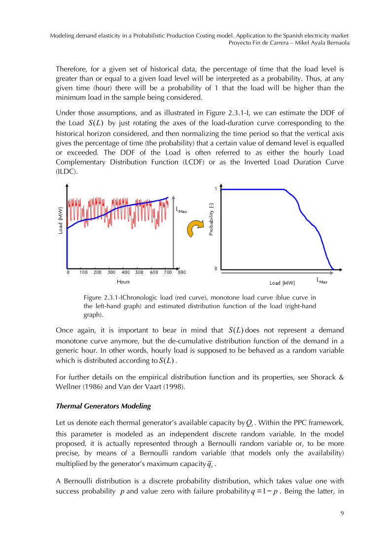
Under those assumptions, and as illustrated in Figure 2.3.1-I, we can estimate the DDF of the Load )(LS by just rotating the axes of the load-duration curve corresponding to the
historical horizon considered, and then normalizing the time period so that the vertical axis gives the percentage of time (the probability) that a certain value of demand level is equalled or exceeded. The DDF of the Load is often referred to as either the hourly Load Complementary Distribution Function (LCDF) or as the Inverted Load Duration Curve (ILDC).
Figure 2.3.1-IChronologic load (red curve), monotone load curve (blue curve in the left-hand graph) and estimated distribution function of the load (right-hand graph).
Once again, it is important to bear in mind that )(LS does not represent a demand
monotone curve anymore, but the de-cumulative distribution function of the demand in a generic hour. In other words, hourly load is supposed to be behaved as a random variable which is distributed according to )(LS .
For further details on the empirical distribution function and its properties, see Shorack & Wellner (1986) and Van der Vaart (1998).
Thermal Generators Modeling
Let us denote each thermal generator’s available capacity by tQ . Within the PPC framework,
this parameter is modeled as an independent discrete random variable. In the model proposed, it is actually represented through a Bernoulli random variable or, to be more precise, by means of a Bernoulli random variable (that models only the availability)
multiplied by the generator’s maximum capacity tq .
A Bernoulli distribution is a discrete probability distribution, which takes value one with success probability p and value zero with failure probability pq −=1 . Being the latter, in
10
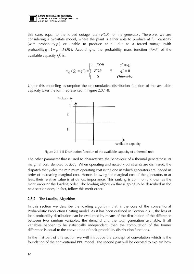
this case, equal to the forced outage rate (FOR ) of the generator. Therefore, we are considering a two-state model, where the plant is either able to produce at full capacity (with probability p ) or unable to produce at all due to a forced outage (with
probability FORpq =−=1 ). Accordingly, the probability mass function (PMF) of the
available capacity tQ is:
−==
0
1
)( * FOR
FOR
qQm ttQt if
Otherwise
q
t
tt
0*
*
==
Under this modeling assumption the de-cumulative distribution function of the available capacity takes the form represented in Figure 2.3.1-II.
Figure 2.3.1-II Distribution function of the available capacity of a thermal unit.
The other parameter that is used to characterize the behaviour of a thermal generator is its
marginal cost, denoted by tMC . When operating and network constraints are dismissed, the
dispatch that yields the minimum operating cost is the one in which generators are loaded in order of increasing marginal cost. Hence, knowing the marginal cost of the generators or at least their relative value is of utmost importance. This ranking is commonly known as the merit order or the loading order. The loading algorithm that is going to be described in the next section does, in fact, follow this merit order.
2.3.2 The Loading Algorithm
In this section we describe the loading algorithm that is the core of the conventional Probabilistic Production Costing model. As it has been outlined in Section 2.3.1, the loss of load probability distribution can be evaluated by means of the distribution of the difference between two random variables: the demand and the total generation available. If all variables happen to be statistically independent, then the computation of the former difference is equal to the convolution of their probability distribution functions.
In the first part of this section we will introduce the concept of convolution which is the foundation of the conventional PPC model. The second part will be devoted to explain how

Modeling demand elasticity in a Probabilistic Production Costing model. Application to the Spanish electricity market Proyecto Fin de Carrera – Mikel Ayala Bernaola
11
it can be applied to analyse the reliability of electric power systems with exclusively thermal generation.
Mathematical Concept of Convolution
We turn now to the important question of determining the distribution of a sum (or difference) of independent random variables in terms of the distributions of the individual constituents.
a. Sum of Discrete Random Variables
Suppose X and Y are two independent discrete random variables with probability mass functions )(xmX and )(ymY . Let YXZ += . We would like to determine the distribution
function )(zmZ of Z . To do this, it is enough to determine the probability that Z takes on
the value z , where z is an arbitrary integer. Suppose that kX = , where k is some integer. Then zZ = if, and only if, kzY −= . So the event zZ = is the union of the pair-wise disjoint events:
)( kX = and )( kzY −=
Where k runs over the integers. Since these events are pair-wise disjoint, we have:
∑∞
−∞=
−=⋅===k
kzYPkXPzZP )()()(
Thus, we have found the distribution function of the random variableZ . This leads to the following definition.
Let X and Y be two independent integer-valued random variables, with distribution
functions )(xmX and )(ymY respectively. Then the convolution of )(xmX and )(ymY is the
distribution function )()()( ymxmzm YXZ ∗= given by the next equation for every integer z .
∑ −⋅=k
YXZ kzmkmzm )()()(
The function )(zmZ is the probability mass function of the random variable YXZ += .
It is easy to prove that the convolution operation is commutative, and it is straightforward to show that it is also associative.
Although the described procedure applies to random integer variables it is not difficult to extend it to any discrete random variable, as long as it is defined for a countably infinite number of discrete values.

12
b. Sum of Continuous Random Variables
Let X and Y be two continuous random variables with density functions )(xf X and )(yfY ,
respectively. Assume that both )(xf X and )(yfY are defined for all real numbers. Then the
convolution YX ff ∗ of Xf and Yf is the function given by
dxxfxzfdyyfyzfzff XYYXYX ⋅⋅−=⋅⋅−=∗ ∫∫+∞
∞−
+∞
∞−
)()()()())((
This definition is analogous to the definition of the convolution of two probability mass functions. Thus it should not be surprising that if X and Y are independent, the density of their sum is the convolution of their densities. That is to say, the sum YXZ += is a random variable with density function )(zfZ , where Zf is the convolution of Xf and Yf .
For further details on the sum of random variables and its properties, see Grinstead & Snell (2003).
Application to Power Systems
As described in Booth (1972), let us introduce the concept of “equivalent load after loading
the first n generating units”, denoted by nEqL . This nEqL , which is a random variable,
represents the load that remains un-served after having loaded the first n groups in the merit order. For instance, the equivalent load after having loaded the first unit in the merit order will be equal to the difference between two random variables, on the one hand the load L
of the system and, on the other hand, the available capacity of the first unit denoted by 1Q .
Explicitly:
11 QLEqL −=
As shown in the previous section, the probability mass function of the load after having loaded the first unit can be computed as follows:
∑ −⋅==k
QEqLEqL klmkmlEqLm )()()(111 1
Generally, the equivalent load after having loaded the first n units can be expressed as follows:
∑=
−=n
t
tn QLEqL1
Or, alternatively:
nnn QEqLEqL −= −1
And its PMF could be computed by carrying the convolution of the variables involved, as expressed next:
Modeling demand elasticity in a Probabilistic Production Costing model. Application to the Spanish electricity market Proyecto Fin de Carrera – Mikel Ayala Bernaola
13
∑ −⋅==−
k
QEqLnEqL klmkmlEqLmnnn
)()()(1
By successively applying the former expression, the distribution functions of the different equivalent loads can be obtained. Obviously, the first equivalent load )0( =n represents the
load of the system, that is to say LEqL =0 . The subsequent equivalent loads represent the
load yet to be covered after dispatching each one of the generators in the system. The last
equivalent load nEqL represents the un-served demand once all of the generators have been
loaded (i.e. the amount of non-served energy).
However, as the available capacity of the thermal units is modeled by means of a binary random variable, the computation of the successive distribution functions of the equivalent load considerably simplifies.
Let us assume that )( 1−nEqLS is the DDF of the un-served load after having loaded the first
1−n groups in the merit order, and that the thn thermal unit can be represented by means of a forced outage rate nFOR and a maximum output nq . Thus, the DDF of the equivalent
load after having loaded the first n groups could be simply computed by applying the following expression:
)()1()()( 11 nnnnnn qlEqLSFORlEqLSFORlEqLS +=⋅−+=⋅== −−
As it can be easily noticed, the DDF of nEqL is equal to the sum of two distinct and rather
meaningful terms:
• On the one hand, the term )( 1 lEqLSFOR nn =⋅ − , which is equal to the distribution
function of the un-served load before loading the thn thermal unit multiplied by its
forced outage rate. In other words, the thn generator will be not available with a probability equal to nFOR and in such an event the un-served load will remain to be
distributed according to )( 1 lEqLS n =− .
• On the other hand, the term )()1( 1 nnn qlEqLSFOR +=⋅− − , which is equal to the
distribution function of the un-served load that would result of the loading of
the thn thermal unit if it were fully available, multiplied by its availability rate. That is
to say, the thn generator will be available with a probability equal to nFOR−1 and in
such an event the un-served load will be distributed according to )( 1 nn qlEqLS +=− .
The following discrete example gives a further insight on how the probabilistic dispatch is carried out. Let us consider the following equivalent load distribution after having loaded the first 1−n units:

14
Figure 2.3.2-I DDF of the demand. Case Example
And let us assume that the available capacity of the thn thermal unit can be modelled by means of the following distribution function:
Figure 2.3.2-II DDF of a thermal unit’s available capacity. Case example
In this case the equivalent load after having loaded the first n generating units can be effortlessly obtained as follows:
The thermal unit will be not available with a probability equal to nFOR and in such an
event the un-served load will remain to be distributed according to )( 1 lEqLS n =− . Therefore
the DDF of the un-served demand will be the one shown in Figure 2.3.2-III.
Prob.
S(EqLn-1)
1
2/3
1/3
2 4 6 [MW]
Prob.
S(Qn)
1
1/2
3 [MW]

Modeling demand elasticity in a Probabilistic Production Costing model. Application to the Spanish electricity market Proyecto Fin de Carrera – Mikel Ayala Bernaola
15
Scenario 1
Figure 2.3.2-III DDF of the demand when generation is not available. Case example
The thermal unit will be available with a probability equal to nFOR−1 and in such an event
the un-served load will be distributed according to )( 1 nn qlEqLS +=− . Thus the DDF of the
un-served demand will be the one shown in Figure 2.3.2.IV.
Scenario 2
Figure 2.3.2-IV DDF of the demand when generation is available. Case example
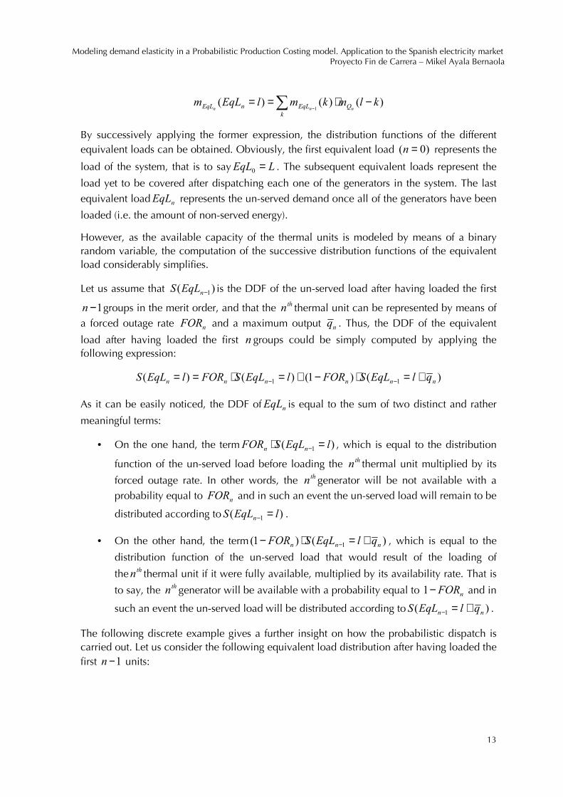
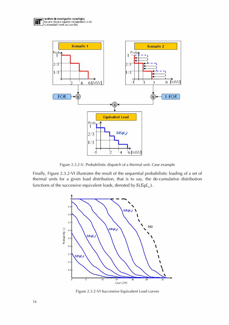
Taking into account both scenarios and their probabilities, the DDF of the un-served load after having loaded the first n units can be obtained straightforwardly. The procedure is depicted in the following figure:
Prob. 1
2/3
1/3
2 4 6 [MW]
Prob1
2/3
1/3
1 3 6 -1 [MW]
16
Figure 2.3.2-V. Probabilistic dispatch of a thermal unit. Case example
Finally, Figure 2.3.2-VI illustrates the result of the sequential probabilistic loading of a set of thermal units for a given load distribution, that is to say, the de-cumulative distribution
functions of the successive equivalent loads, denoted by )( nEqLS .
Figure 2.3.2-VI Successive Equivalent Load curves
Modeling demand elasticity in a Probabilistic Production Costing model. Application to the Spanish electricity market Proyecto Fin de Carrera – Mikel Ayala Bernaola
17
2.3.3 Basic Results Provided
The major outputs that can be calculated by means of this model include reliability measures, expected production schedules, expected production costs and marginal price probabilistic distributions.
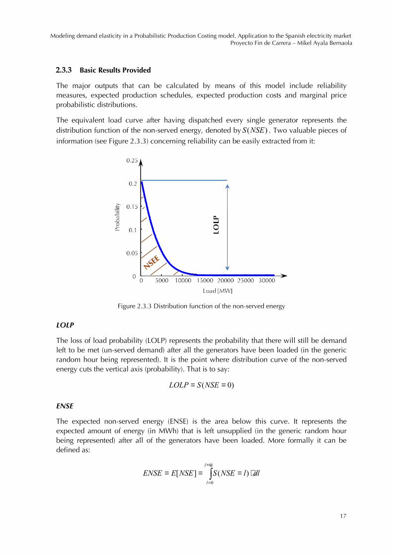
The equivalent load curve after having dispatched every single generator represents the distribution function of the non-served energy, denoted by )(NSES . Two valuable pieces of
information (see Figure 2.3.3) concerning reliability can be easily extracted from it:
Figure 2.3.3 Distribution function of the non-served energy
LOLP
The loss of load probability (LOLP) represents the probability that there will still be demand left to be met (un-served demand) after all the generators have been loaded (in the generic random hour being represented). It is the point where distribution curve of the non-served energy cuts the vertical axis (probability). That is to say:
)0( == NSESLOLP
ENSE
The expected non-served energy (ENSE) is the area below this curve. It represents the expected amount of energy (in MWh) that is left unsupplied (in the generic random hour being represented) after all of the generators have been loaded. More formally it can be defined as:
dllNSESNSEEENSE
l
l
⋅=== ∫+∞=
=0
)(][
18
LOLE
The loss of load expectancy (LOLE) expresses the expected number of hours within a certain period in which the system load is expected to exceed the available electricity generation capacity; see Van Wijck (1990). Once the LOLP has been determined, calculating the LOLE is not difficult at all.
Let ΨA be the total number of hours in the time scope analyzed. The number of hours in which the load will exceed the generation capacity will be given by a Binomial Distribution
of parameters Ψ= An and LOLPp = . The LOLE will be equal to the expected value of that
distribution. That is to say:
Ψ⋅= ALOLPLOLE
Traditionally, a reliability standard of one day in ten years has been established in electric systems; see FERC (2010).
Expected energy supplied by a unit
It can be easily checked that the expected value of the energy produced by a given unit (in a generic hour) can be computed as the difference between the NSEE before and after dispatching that unit, as shown in the next equation:
dllEqLSdllEqLSEE
l
l
n
l
l
nn ⋅=−⋅== ∫∫+∞=
=
+∞=
=−
00
1 )()(][
Probability of being marginal
As it will be shown further in this chapter, in Section 2.7, the probability of a plant being marginal can be directly obtained within the PPC framework as follows:
)0()0( 1arg =−== − nn
n
inalM EqLSEqLSp
2.4 The Hydro-Thermal System Model
As put across by Batlle (2002), modelling hydro plants is clearly one of the most challenging tasks that can be thought of in the electricity sector. In fact, even the purely theoretical design of a model covering all of its peculiarities is hard to conceive.
For instance, the function that relates, for each plant, the amount of energy that can be generated to the volume of stored water is tremendously complex (i.e. it is non-linear and depends on the shape of the reservoir and even on the water of flow released). A further handicap is the fact that hydro units are commonly connected with other up and down-stream storage units (both in series and in parallel) what introduces spatial and time-linking constraints.
Hence, it is clear that any representation of hydro production must contain strong modelling simplifications that, nonetheless, allow for considering the fact that hydro plants are energy

Modeling demand elasticity in a Probabilistic Production Costing model. Application to the Spanish electricity market Proyecto Fin de Carrera – Mikel Ayala Bernaola
19
constrained (i.e. it is not possible to produce at maximum power whenever desired). Section 2.4.1 starts describing the assumptions undertaken by the modelling approach. We next show, in section 2.4.2, how hydro units can be incorporated to the PPC frame work. We conclude discussing the validity of the model proposed.
2.4.1 Hydro Units Modelling
As it has been previously noted, the remarkable complexity of the hydroelectric system imposes the need for reduced representations of the hydro units. The modelling assumptions carried out in order to make possible the medium and long term analysis proposed in this dissertation are based on the work of Batlle (2002).
Following the approach proposed there, a group of hydro plants set in the same river basin and operated by the same firm are synthesized into a unique plant. From now on, we will refer to these composite representations as hydro plants.
Each one of those hydro plants is characterized by three parameters assumed to be constant for each time period ψ in which the time scope Ψ is divided:
• ≡ψhq Maximum capacity constraint of hydro plant h in periodψ .
• ≡ψh
q Minimum output (run-of-the-river power) of hydro h in periodψ .
• ≡ψhe Available energy at hydro plant h in periodψ .
As opposed to thermal plants, the three parameters that define the behaviour of each hydro unit are different for each period of timeψ . While the operating constraints of the thermal
plants can be considered to be constant through the whole time scope of analysis, the ones that characterize the production of hydro plants are greatly time-dependent.
Another fundamental issue regarding hydro units modelling is the fact that no forced outage rate is considered. Given that it is not significant compared their energy restriction, it is neglected.
The model inputs are derived from historical values using the GEHA (Generador de
Escenarios Hidráulicos Aleatorios, hydro production random scenario generator) developed by Batlle (2002). The GEHA consists basically of:
• A time series model that generates a series of hydro energy produced in each period in the whole system.
• A module that distributes that energy production among all the hydro units according to randomly sampled historical data.
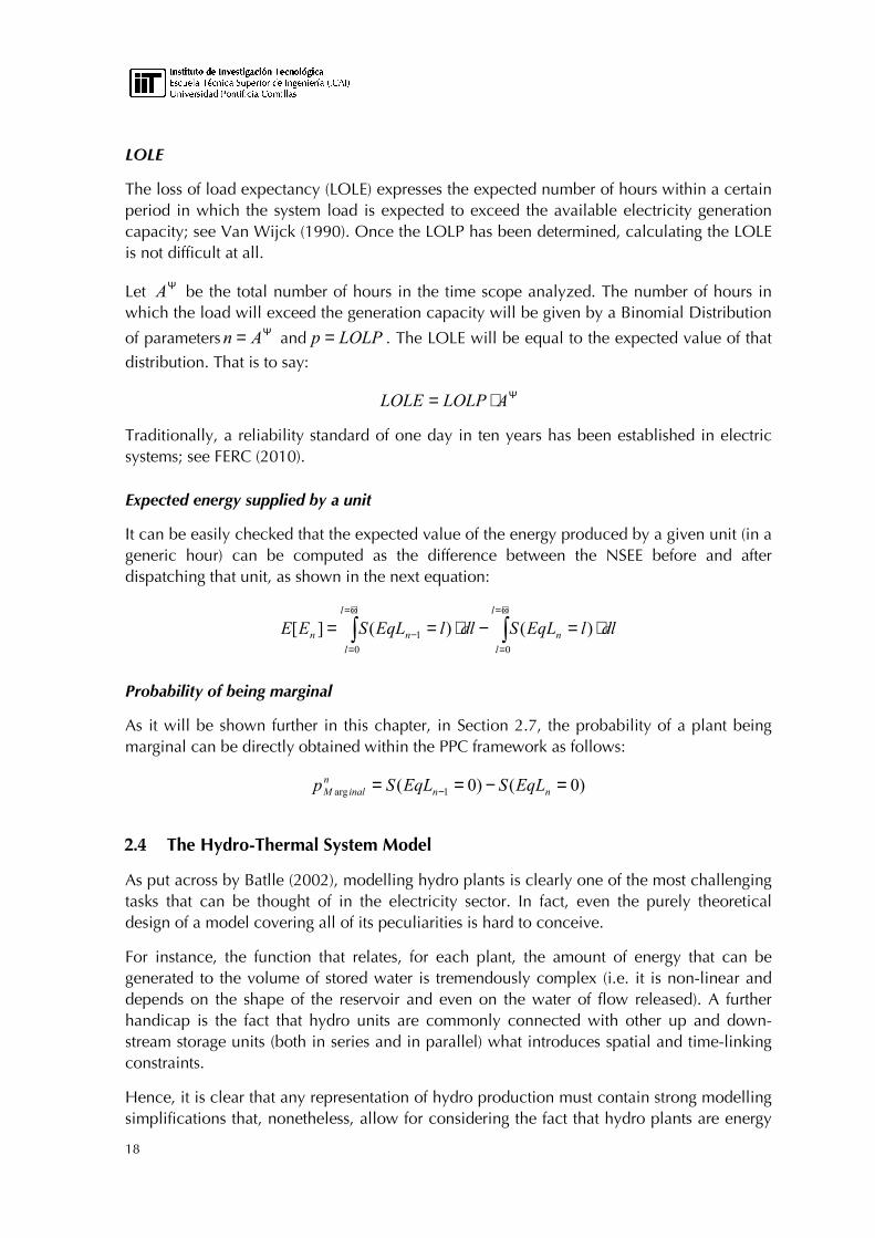
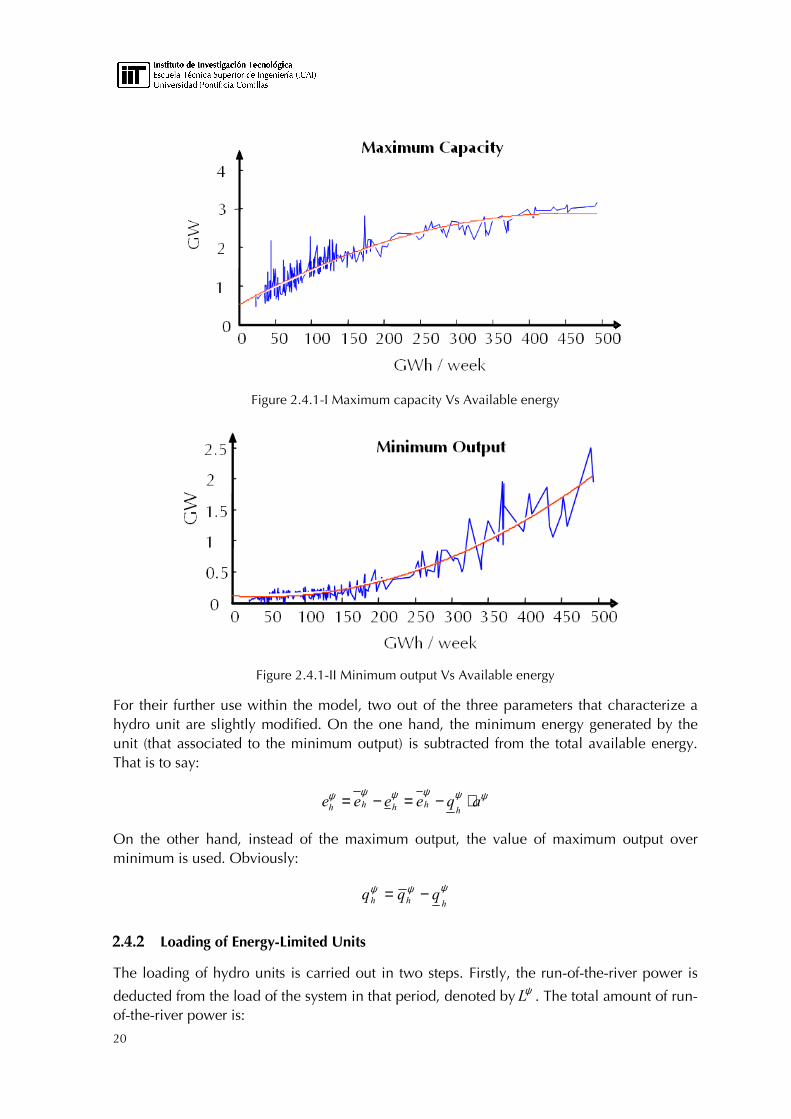
• A regression model that relates the energy produced by each hydro unit in a period with its maximum and minimum capacity values for that period, as shown in Figure 2.4.1-I and in Figure 2.4.1-II respectively.
20
Figure 2.4.1-I Maximum capacity Vs Available energy
Figure 2.4.1-II Minimum output Vs Available energy
For their further use within the model, two out of the three parameters that characterize a hydro unit are slightly modified. On the one hand, the minimum energy generated by the unit (that associated to the minimum output) is subtracted from the total available energy. That is to say:
ψψψψψψ aqeeeeh
hhhh ⋅−=−=
On the other hand, instead of the maximum output, the value of maximum output over minimum is used. Obviously:
ψψψhhh qqq −=
2.4.2 Loading of Energy-Limited Units
The loading of hydro units is carried out in two steps. Firstly, the run-of-the-river power is
deducted from the load of the system in that period, denoted by ψL . The total amount of run-of-the-river power is:

Modeling demand elasticity in a Probabilistic Production Costing model. Application to the Spanish electricity market Proyecto Fin de Carrera – Mikel Ayala Bernaola
21
∑=
=H
hhH
qQ1
ψψ
And therefore, the distribution of the load after having loaded the minimum output of every hydro unit will be computed as follows:
)()(ψψψ
ψHQ
QlLSlLSH
+===
The loading of the run-of-the-river power is illustrated in Figure 2.4.2-I.
Figure 2.4.2-I Loading of the run-of-the river output
Secondly, the remaining available energy of each hydro unit ψhe is loaded. Since plants are
loaded sequentially (one after another), as a first step, they have to be sort according to the merit order that is described later in this section. Hydro plants are then scheduled attempting to make the most of their available energy. The loading algorithm proceeds as follows:
Step 0. Let us denote ψψH
QL by ψ
1−nEqL
Step 1. The hydro unit is supposed to produce at full capacity (over minimum) if the equivalent load is equal to or higher than it. On the other hand, if the load is lower than the capacity the production is supposed to be equal to the load. Accordingly, the distribution function of the load after having loaded the hydro unit would be:
+==
==−
−
)(
)()(
1
1
ψψ
ψψ
hn
n
nqlEqLS
lEqLSlEqLS if
l
l
≤<0
0
Step 2. The expected value of the energy that the hydro unit would produce if it were dispatched in that position is computed as follows:
22
dllEqLSdllEqLSEE
l
l
n
l
l
nh ⋅=−⋅== ∫∫+∞=
=
+∞=
=−
00
1 )()(][ ψψ
Step 3. If ψhh eEE ≤][ , that is to say, if the expected energy production does not
exceed the available energy, the hydro unit is scheduled in that position. Therefore, the equivalent load to be met by the remaining generating units will be the one calculated in Step 2. Additionally, the values of the indexes n and h are updated (they are increased in one unit) and the dispatch algorithm goes back to Step 1.
If ψhh eEE >][ , that is to say, if there is not enough available energy, the
equivalent load remains to be ψ1−nEqL and the algorithm proceeds to Step 4
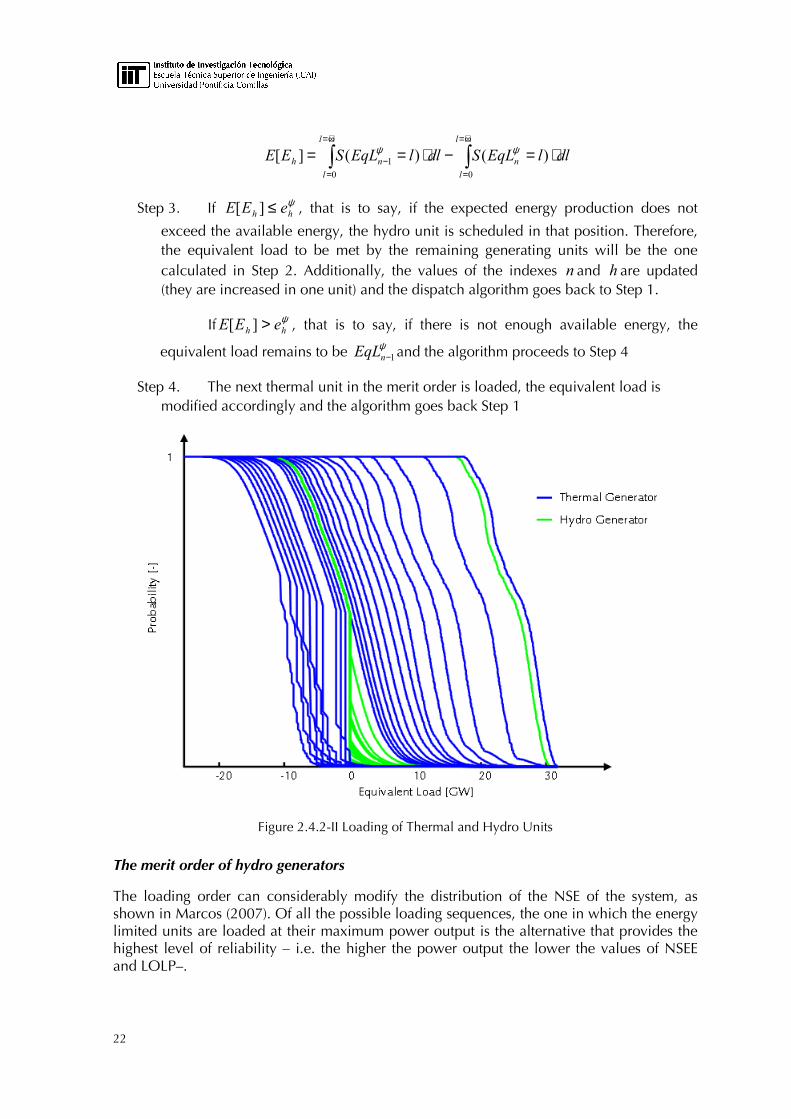
Step 4. The next thermal unit in the merit order is loaded, the equivalent load is modified accordingly and the algorithm goes back Step 1
Figure 2.4.2-II Loading of Thermal and Hydro Units
The merit order of hydro generators
The loading order can considerably modify the distribution of the NSE of the system, as shown in Marcos (2007). Of all the possible loading sequences, the one in which the energy limited units are loaded at their maximum power output is the alternative that provides the highest level of reliability – i.e. the higher the power output the lower the values of NSEE and LOLP–.
Modeling demand elasticity in a Probabilistic Production Costing model. Application to the Spanish electricity market Proyecto Fin de Carrera – Mikel Ayala Bernaola
23
Consequently, hydro units are ranked according to the total number of hours that they can produce at full capacity. For each unit, that parameter is calculated as:
ψ
ψψτ
h
hh
q
e=
2.4.3 Validity of the Expected Energy Convolution Model
As highlighted by Marcos (2007), loading energy limited generators using all the energy available in each unit as an expected value (as is the case of most probabilistic models applied to power systems) leads to unfeasible scenarios (due to the lack of available energy) that must be taken into account.
Energy supplied by a hydro unit in a given period
Let ψhQ be a random variable that represents the output of hydro unit h in any given hour of
periodψ (that is composed of ψa hours). Obviously, the output of that unit can be obtained
as the difference of two random variables as:
nnh EqLEqLQ −= −1ψ
Therefore it is possible to determine the PMF of the hourly output ψhQ by convolution
recalling to the following expression:
)()()( 11 nEqLnEqLhQEqLmEqLmQm
nnh
−∗= −−−
ψψ
Thus, the energy supplied by that hydro unit in periodψ could be represented by means of
another random variable, denoted by ψhE . Since the outputs of different hours are supposed
to be independent, the energy produced by the hydro unit could be obtained as follows:
timesa
ahhhh QQQE
ψ
ψψψψψ +++= ...
21
Or, in terms of PMF as:
timesa
ahhhhE
QmQmQmEmh
ψ
ψψψψψψ )(...)()()(
21∗∗∗=
The former expression requires a remarkable computational effort. However, given that the
number of hours in a period is usually large enough )30( >ψa , and that the hourly outputs ψhQ are supposed to be behaved as independent and identically distributed random
variables, the computation of the distribution function of the energy supplied by a hydro unit considerably simplifies.
24
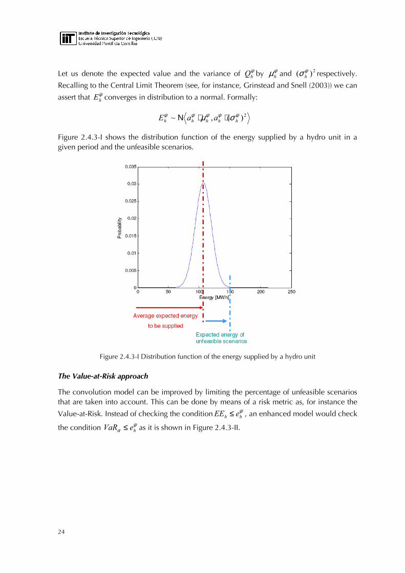
Let us denote the expected value and the variance of ψhQ by ψµh and 2)( ψσ h respectively.
Recalling to the Central Limit Theorem (see, for instance, Grinstead and Snell (2003)) we can
assert that ψhE converges in distribution to a normal. Formally:
2)(,~ ψψψψψ σµ hhhhh aaE ⋅⋅Ν
Figure 2.4.3-I shows the distribution function of the energy supplied by a hydro unit in a given period and the unfeasible scenarios.
Figure 2.4.3-I Distribution function of the energy supplied by a hydro unit
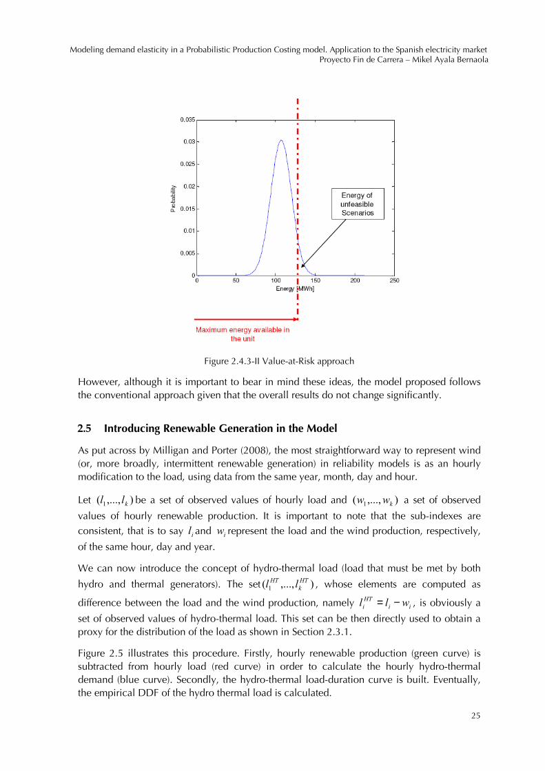
The Value-at-Risk approach
The convolution model can be improved by limiting the percentage of unfeasible scenarios that are taken into account. This can be done by means of a risk metric as, for instance the
Value-at-Risk. Instead of checking the condition ψhh eEE ≤ , an enhanced model would check
the condition ψα heVaR ≤ as it is shown in Figure 2.4.3-II.
Modeling demand elasticity in a Probabilistic Production Costing model. Application to the Spanish electricity market Proyecto Fin de Carrera – Mikel Ayala Bernaola
25
Figure 2.4.3-II Value-at-Risk approach
However, although it is important to bear in mind these ideas, the model proposed follows the conventional approach given that the overall results do not change significantly.
2.5 Introducing Renewable Generation in the Model
As put across by Milligan and Porter (2008), the most straightforward way to represent wind (or, more broadly, intermittent renewable generation) in reliability models is as an hourly modification to the load, using data from the same year, month, day and hour.
Let ),...,( 1 kll be a set of observed values of hourly load and ),...,( 1 kww a set of observed
values of hourly renewable production. It is important to note that the sub-indexes are
consistent, that is to say il and iw represent the load and the wind production, respectively,
of the same hour, day and year.
We can now introduce the concept of hydro-thermal load (load that must be met by both
hydro and thermal generators). The set ),...,( 1HT
k
HT ll , whose elements are computed as
difference between the load and the wind production, namely ii
HT
i wll −= , is obviously a
set of observed values of hydro-thermal load. This set can be then directly used to obtain a proxy for the distribution of the load as shown in Section 2.3.1.
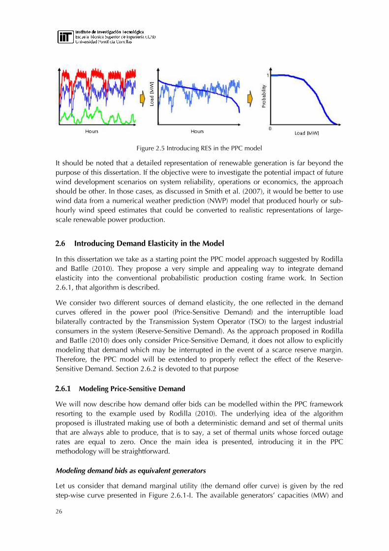
Figure 2.5 illustrates this procedure. Firstly, hourly renewable production (green curve) is subtracted from hourly load (red curve) in order to calculate the hourly hydro-thermal demand (blue curve). Secondly, the hydro-thermal load-duration curve is built. Eventually, the empirical DDF of the hydro thermal load is calculated.
26
Figure 2.5 Introducing RES in the PPC model
It should be noted that a detailed representation of renewable generation is far beyond the purpose of this dissertation. If the objective were to investigate the potential impact of future wind development scenarios on system reliability, operations or economics, the approach should be other. In those cases, as discussed in Smith et al. (2007), it would be better to use wind data from a numerical weather prediction (NWP) model that produced hourly or sub-hourly wind speed estimates that could be converted to realistic representations of large-scale renewable power production.
2.6 Introducing Demand Elasticity in the Model
In this dissertation we take as a starting point the PPC model approach suggested by Rodilla and Batlle (2010). They propose a very simple and appealing way to integrate demand elasticity into the conventional probabilistic production costing frame work. In Section 2.6.1, that algorithm is described.
We consider two different sources of demand elasticity, the one reflected in the demand curves offered in the power pool (Price-Sensitive Demand) and the interruptible load bilaterally contracted by the Transmission System Operator (TSO) to the largest industrial consumers in the system (Reserve-Sensitive Demand). As the approach proposed in Rodilla and Batlle (2010) does only consider Price-Sensitive Demand, it does not allow to explicitly modeling that demand which may be interrupted in the event of a scarce reserve margin. Therefore, the PPC model will be extended to properly reflect the effect of the Reserve-Sensitive Demand. Section 2.6.2 is devoted to that purpose
2.6.1 Modeling Price-Sensitive Demand
We will now describe how demand offer bids can be modelled within the PPC framework resorting to the example used by Rodilla (2010). The underlying idea of the algorithm proposed is illustrated making use of both a deterministic demand and set of thermal units that are always able to produce, that is to say, a set of thermal units whose forced outage rates are equal to zero. Once the main idea is presented, introducing it in the PPC methodology will be straightforward.
Modeling demand bids as equivalent generators
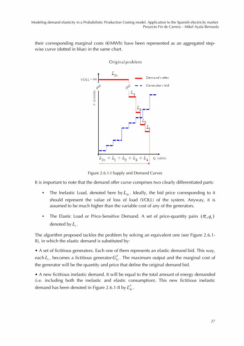
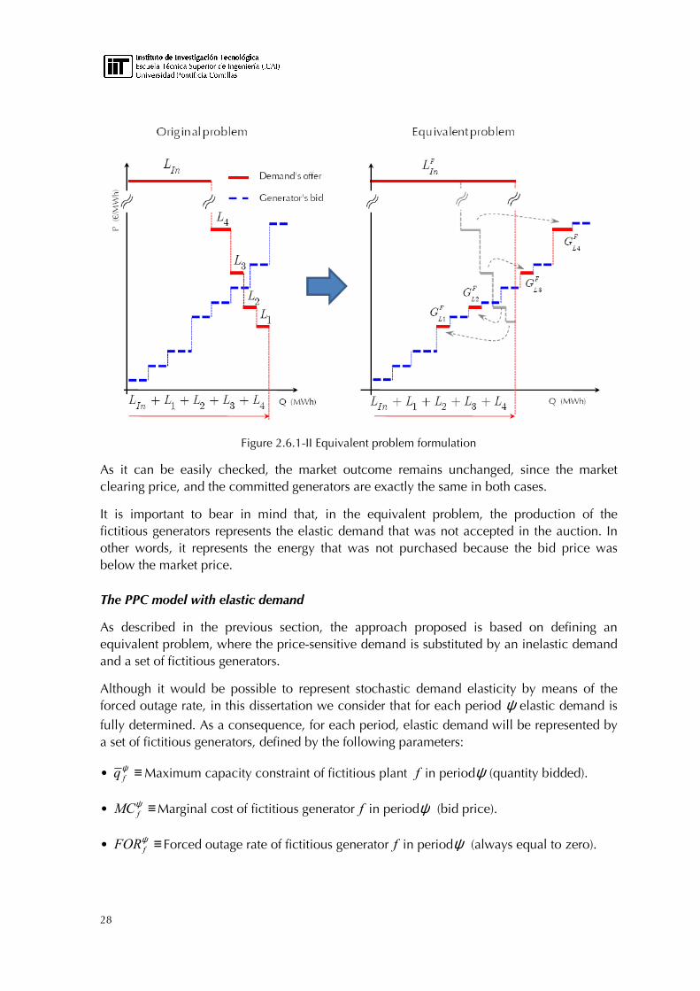
Let us consider that demand marginal utility (the demand offer curve) is given by the red step-wise curve presented in Figure 2.6.1-I. The available generators’ capacities (MW) and
Modeling demand elasticity in a Probabilistic Production Costing model. Application to the Spanish electricity market Proyecto Fin de Carrera – Mikel Ayala Bernaola
27
their corresponding marginal costs (€/MWh) have been represented as an aggregated step-wise curve (dotted in blue) in the same chart.
Figure 2.6.1-I Supply and Demand Curves
It is important to note that the demand offer curve comprises two clearly differentiated parts:
• The Inelastic Load, denoted here by InL . Ideally, the bid price corresponding to it
should represent the value of loss of load (VOLL) of the system. Anyway, it is assumed to be much higher than the variable cost of any of the generators.
• The Elastic Load or Price-Sensitive Demand. A set of price-quantity pairs ),( ii qπ
denoted by iL .
The algorithm proposed tackles the problem by solving an equivalent one (see Figure 2.6.1-II), in which the elastic demand is substituted by:
• A set of fictitious generators. Each one of them represents an elastic demand bid. This way,
each iL , becomes a fictitious generator F
LiG . The maximum output and the marginal cost of
the generator will be the quantity and price that define the original demand bid.
• A new fictitious inelastic demand. It will be equal to the total amount of energy demanded (i.e. including both the inelastic and elastic consumption). This new fictitious inelastic
demand has been denoted in Figure 2.6.1-II by F
InL .
28
Figure 2.6.1-II Equivalent problem formulation
As it can be easily checked, the market outcome remains unchanged, since the market clearing price, and the committed generators are exactly the same in both cases.
It is important to bear in mind that, in the equivalent problem, the production of the fictitious generators represents the elastic demand that was not accepted in the auction. In other words, it represents the energy that was not purchased because the bid price was below the market price.
The PPC model with elastic demand
As described in the previous section, the approach proposed is based on defining an equivalent problem, where the price-sensitive demand is substituted by an inelastic demand and a set of fictitious generators.
Although it would be possible to represent stochastic demand elasticity by means of the forced outage rate, in this dissertation we consider that for each period ψ elastic demand is
fully determined. As a consequence, for each period, elastic demand will be represented by a set of fictitious generators, defined by the following parameters:
• ≡ψfq Maximum capacity constraint of fictitious plant f in periodψ (quantity bidded).
• ≡ψfMC Marginal cost of fictitious generator f in periodψ (bid price).
• ≡ψfFOR Forced outage rate of fictitious generator f in periodψ (always equal to zero).

Modeling demand elasticity in a Probabilistic Production Costing model. Application to the Spanish electricity market Proyecto Fin de Carrera – Mikel Ayala Bernaola
29
2.6.2 .Modeling Reserve-Sensitive Demand
In order to consider the load shedding capability bilaterally contracted by the system operator we propose the following methodology.
For each period ψ in which the time scope of analysis Ψ is divided, the interruptible load
)(IL is placed in the supply function merit order allowing a certain level of reserve margin
)(RM specified by the Transmission System Operator. That is to say, IL is modelled as a
fictitious generator characterized by the following parameters:
• ≡ψILq Maximum capacity constraint of fictitious plant IL . It is equal to the total
interruptible load (in MW).
• ≡ψILFOR Forced outage rate of fictitious generator IL (always equal to zero).
• ≡ψILMC Marginal cost of fictitious generator IL in periodψ . It is set in such away that the
position of the fictitious generator IL allows for the desired level of reserve margin.
The reserve margin for each period, namely ψRM (in MW), is calculated as a given
percentage )( RMε of the maximum load of that period, denoted by ψMaxl . Formally:
ψψ ε MaxRM lRM ⋅=
Figure 2.6.2 illustrates how the interruptible load is included in the supply function as a fictitious generator.
Figure 2.6.2 Reserve Sensitive Demand

30
2.7 Measuring the Value of Non-Purchased Energy
In this section, we present a methodology for constructing the distribution function of the so called Value of Non-Purchased Energy within the PPC framework. First, we recall the background of the VNPE and its importance. Next, we define it in a precise and concise way. And, eventually we provide a general formulation of the VNPE calculation algorithm.
2.7.1 The Background of the Concept
As highlighted in (Rodilla, 2010), classical reliability measures such as the Loss of Load Probability (LOLP), and the Expected Non-Served Energy (ENSE) leave aside very meaningful information when used to assess the performance of a system where elastic demand plays a significant role. As a matter of fact, in a fully elastic demand scenario, the value of the ENSE is, according to its traditional definition, always equal to zero. Consequently, a permanent scenario of severe scarcity could be obscured by the use of the aforementioned metrics.
In order to reflect the elastic consumption in the performance measure, the evaluation of the distribution function of what was termed as the value of the non-purchased energy (VNPE) was proposed. The purpose of this section is to illustrate how it can be calculated in a real-size case.
2.7.2 Brief Overview of the VNPE Concept
Let us characterize the demand by means of a set Ω of price-quantity pairs ),( ii qπ where:
iπ stands for the bid price (i.e. the highest price the buyer is willing to pay).
iq denotes the quantity bidded.
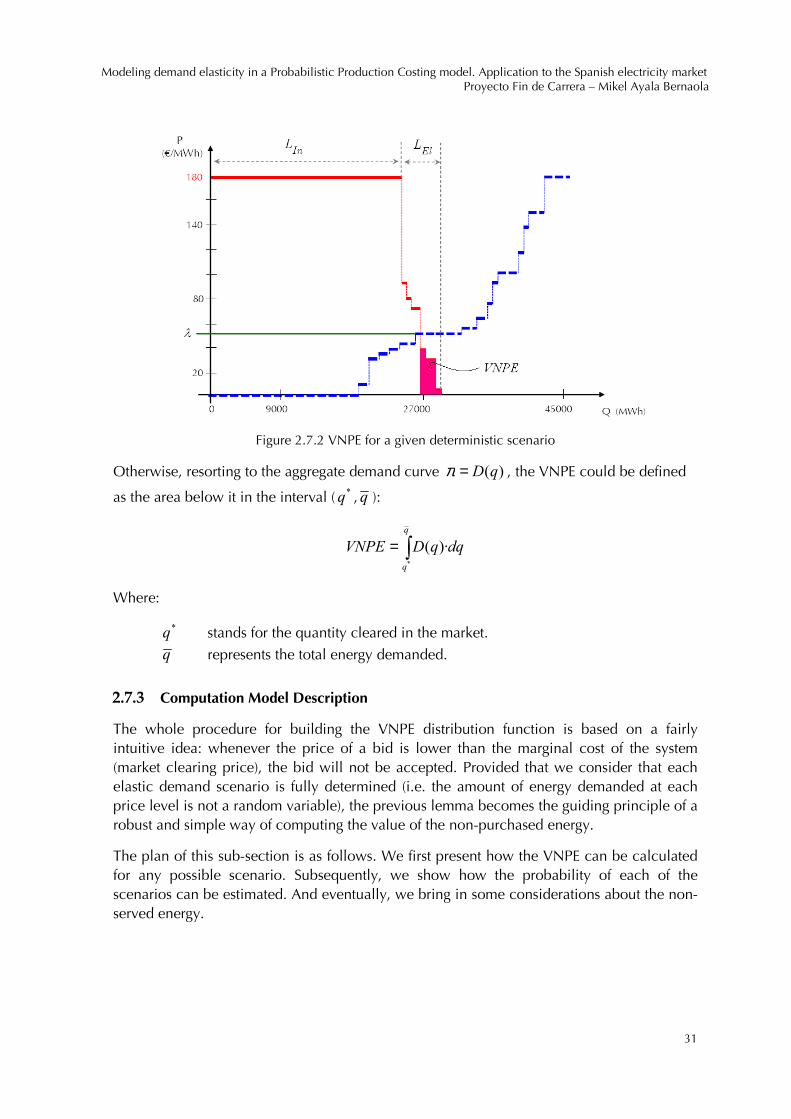
We can define the term “value of a bid” as the quantity demanded multiplied by the bid price. Thus, for a given demand and supply deterministic scenario, the value of the non-purchased energy will be the total sum of the values of the bids that are not accepted.
Modeling demand elasticity in a Probabilistic Production Costing model. Application to the Spanish electricity market Proyecto Fin de Carrera – Mikel Ayala Bernaola
31
Figure 2.7.2 VNPE for a given deterministic scenario
Otherwise, resorting to the aggregate demand curve )(qD=π , the VNPE could be defined
as the area below it in the interval ( *q ,q ):
∫=q
q
dqqDVNPE*
)·(
Where:
*q stands for the quantity cleared in the market.
q represents the total energy demanded.
2.7.3 Computation Model Description
The whole procedure for building the VNPE distribution function is based on a fairly intuitive idea: whenever the price of a bid is lower than the marginal cost of the system (market clearing price), the bid will not be accepted. Provided that we consider that each elastic demand scenario is fully determined (i.e. the amount of energy demanded at each price level is not a random variable), the previous lemma becomes the guiding principle of a robust and simple way of computing the value of the non-purchased energy.
The plan of this sub-section is as follows. We first present how the VNPE can be calculated for any possible scenario. Subsequently, we show how the probability of each of the scenarios can be estimated. And eventually, we bring in some considerations about the non-served energy.

32
Value of Non-Purchased Energy Calculation
a. The marginal plant is a thermal or hydro generator
Let us firstly assume that: the marginal unit is either thermal or hydro (in other words, not
fictitious); that additionally, it will be marginal with a probability equal to inalMp arg ; and that
the market clearing price of the system isλ . In such an event, the VNPE could be easily computed as follows:
∑Γ∈
=),(
·ii q
ii qVNPEπ
π /),( λππ <Ω∈=Γ iii q
Therefore, the value of the non-purchased energy will be the one calculated above with a
probability equal to inalMp arg .
b. The marginal plant is a fictitious generator
If a fictitious generator happens to be the marginal one, that is to say, if a demand bid represented by a so-called fictitious generator is partially accepted, the calculation of the VNPE differs slightly. In addition to the bids that were fully rejected, it is necessary to take into account the value of the bid that was partially turned down.
In order to do so, we make use of the probability mass function (PMF) of the production of the fictitious generator. Assuming that the production of a fictitious generator can be
represented by means of a discrete random variable denoted by fQ , that function gives the
probability that the former is exactly equal to some value.
Once we have obtained the PMF )( fQ Qmf
, computing the VNPE and probability of each
scenario is straightforward. Formally:
∑Γ∈
+=),(
* ··ii qp
iiff qqVNPE ππ /),( λππ <Ω∈=Γ iii q
Where:
fπ stands for the bid price of the fictitious marginal generator.
*
fq denotes the quantity not purchased (production of the fictitious generator).
The value of the non-purchased energy will be the one calculated above with a probability
equal to )( *
ffQ qQmf
= for every value of fQ so that the fictitious generator is marginal.
That is to say, for every *
ff qQ = such that ff qq << *0 , where fq stands for the maximum
output of the fictitious generator (quantity demanded).
Modeling demand elasticity in a Probabilistic Production Costing model. Application to the Spanish electricity market Proyecto Fin de Carrera – Mikel Ayala Bernaola
33
Scenario Probability Estimation
a. Probability of being marginal
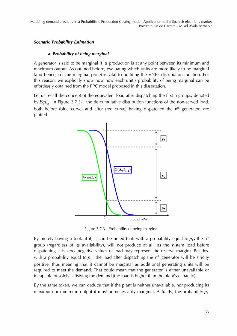
A generator is said to be marginal if its production is at any point between its minimum and maximum output. As outlined before, evaluating which units are more likely to be marginal (and hence, set the marginal price) is vital to building the VNPE distribution function. For this reason, we explicitly show now how each unit’s probability of being marginal can be effortlessly obtained from the PPC model proposed in this dissertation.
Let us recall the concept of the equivalent load after dispatching the first n groups, denoted
by nEqL . In Figure 2.7.3-I, the de-cumulative distribution functions of the non-served load,
both before (blue curve) and after (red curve) having dispatched the nth generator, are plotted.
Figure 2.7.3-I Probability of being marginal
By merely having a look at it, it can be noted that: with a probability equal to 1p , the nth
group (regardless of its availability), will not produce at all, as the system load before dispatching it is zero (negative values of load may represent the reserve margin). Besides,
with a probability equal to 3p , the load after dispatching the nth generator will be strictly
positive, thus meaning that it cannot be marginal as additional generating units will be required to meet the demand. That could mean that the generator is either unavailable or incapable of solely satisfying the demand (the load is higher than the plant’s capacity).
By the same token, we can deduce that if the plant is neither unavailable, nor producing its
maximum or minimum output it must be necessarily marginal. Actually, the probability 2p

34
represents the likelihood of that happening. Said in a different and more concise way, the nth
group will be marginal with a probability equal to 2p .
In conclusion, measuring each generator’s probability of being marginal can be reduced to nothing more than plainly subtracting two numbers: the intercepts of both the de-cumulative distribution function of the equivalent load before dispatching the generator (denoted by
)( 1−nEqLS ) and the de-cumulative distribution function of the equivalent load after
dispatching it (denoted by )( nEqLS ) with the vertical axis. Explicitly, the nth generator will
be marginal with a probability equal to:
)0()0( 1arg =−== − nn
n
inalM EqLSEqLSp
b. Non-Purchased Energy Probability Mass Function
In order to be treated within the model, the inelastic load is quantized according to a specified resolution, and so are the supply offers and the elastic bids. As a result, discrete random variables can be proxy for both the production of the generators and the n equivalent loads.
As pointed out above, determining the probability mass function of the production of the fictitious generators is key to building the VNPE distribution function. We will now try to shortly describe how it is obtained from the PPC model by recourse to an example.
Let )( nEqL EqLmn
be the probability mass function of the equivalent load after dispatching
the first n groups.
Figure 2.7.3-II Probability mass function of the Equivalent Load
And let us assume now that the following generator in the merit order is a fictitious one (a
demand bid) of capacity fq . Obviously, if the equivalent load is either zero or negative, the
output of the fictitious generator will be zero. In addition to that, if the load is higher or
Modeling demand elasticity in a Probabilistic Production Costing model. Application to the Spanish electricity market Proyecto Fin de Carrera – Mikel Ayala Bernaola
35
equal to the capacity, the output of the generator will be its capacity. And, needless to say, in any other case, the production will be equal to the load and, by the way, the fictitious generator will be marginal.
More formally, the PMF of the production of a fictitious generator that is dispatched after the first n units can be defined as a piecewise function:
==
∑
∑
∞<≤
≤<∞−
nF
n
n
n
n
f
EqLq
nEqL
nEqL
EqL
nEqL
ffQ
EqLm
EqLm
EqLm
qQm
)(
)(
)(
)(0
* if f
ff
f
f
q
q
q
=<<
=
*
*
0
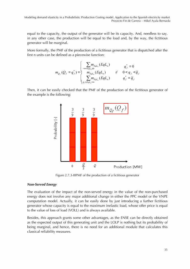
0
Then, it can be easily checked that the PMF of the production of the fictitious generator of the example is the following:
Figure 2.7.3-IIIPMF of the production of a fictitious generator
Non-Served Energy
The evaluation of the impact of the non-served energy in the value of the non-purchased energy does not involve any major additional change in either the PPC model or the VNPE computation model. Actually, it can be easily done by just introducing a further fictitious generator whose capacity is equal to the maximum inelastic load, whose offer price is equal to the value of loss of load (VOLL) and is always available.
Besides, this approach grants some other advantages, as the ENSE can be directly obtained as the expected output of this generating unit and the LOLP is nothing but its probability of being marginal, and hence, there is no need for an additional module that calculates this classical reliability measures.
36
2.8 Conclusions
In this chapter we have formulated a Probabilistic Production Costing model to carry out reliability assessments of power generation systems in electricity markets where elastic demand plays a significant role. The model described is able to cope with a variety of peculiarities of electricity wholesale markets.
Moreover, the proposed formulation meets the following modelling challenges:
• Firstly, the model allows for analysis in a conventional thermal generation system with fully inelastic load.
• Secondly, the conventional PPC model has been adapted for loading energy limited units.
• Thirdly, the conventional PPC model has been extended with regard to taking into account intermittent renewable generation.
• Fourthly, an equivalent load and generation model has been constructed to integrate price sensitive demand into the conventional PPC model.
• Fifthly, the PPC model has been adjusted to properly reflect the effect of the reserve-sensitive demand.
• Sixthly, an algorithm to compute the distribution function of the Value of the Non-Purchased Energy has been implemented within the PPC frame-work.
This PPC model will be used in Chapter 4 to carry out a reliability assessment of the Spanish electricity market.
2.9 References
Ayoub, A. K. & A. D. Patton (1976). ”A Frequency and Duration Method for Generating System Reliability Evaluation”. IEEE Transactions on Power Apparatus and Systems, vol. 95, iss. 6, part 1, pp. 1929-1933, 1976.
Baleriaux, H., E. Jamoulle and F. Linard de Guertechin (1967). “Simulation de l’Explotation d’un Parc de Machines Thermiques de Production d’Electricité Couplé à des Stations de Pompage,” Revue E, Vol. V, No. 7, pp. 225-245, 1967.
Batlle, C. (2002). “A Model for Electricity Generation Risk Analysis”. PhD Thesis. IIT, Universidad Pontificia Comillas, 2002.
Booth, R. R. (1962). “Power System Simulation Model Based on Probability Analysis,” IEEE Transactions on Power Apparatus and Systems, PAS-91, pp. 62-69, January/February 1972.
Conejo, A. J. (1987) “Optimal Utilization of Electricity Storage Reservoirs: Efficient Algorithms Embedded in Probabilistic Production Costing Models”. M. S. Thesis. Massachusetts Institute of Technology. August 1987.
Modeling demand elasticity in a Probabilistic Production Costing model. Application to the Spanish electricity market Proyecto Fin de Carrera – Mikel Ayala Bernaola
37
Conejo, A. J., I. J. Pérez-Arriaga, A. Ramos and A. Santamaría (1985). “Evaluation of the Impact of Solar Thermal Generation on the Reliability and Economics of an Electrical Utility System“, IEEE Mediterranean Electrotechnical Conference. MELECON '85 4: 167-173 A. Luque, A.R. Figueiras Vidal, D. Nobili (eds.) Elsevier Science Publishers B.V. Madrid, Spain October 1985.
FERC, (2010). “Planning Resource Adequacy Assessment Reliability Standard”. Federal Energy Regulatory Commission, Notice of Proposed Rulemaking, October 2010.
Finger, S. (1979). “Electric power system production costing and reliability analysis including hydro-electric, storage, and time dependent power plants”. MIT Energy Laboratory Technical Report #MIT-EL-79-006, February 1979
Garver, L. L. (1966). “Effective Load Carrying Capability of Generating Units” IEEE Transactions on Power Apparatus and Systems, Vol. PAS-85, no. 8, pp. 910-919, August 1966.
Grinstead, C.M. and J.L. Snell (2003). “Introduction to Probability, 2nd Edition”. American Mathematical Society, pp. 285-304, 2003.
Halperin, H. & H. A. Adler (1958). “Determination of reserve generating capability”. Trans. AIEE, vol. 77, pt. III, pp. 530-544, August 1958.
Invernizzi, A., G. Manzoni and A. Rivoiro (1988). “Probabilistic simulation of generating system operation including seasonal hydro reservoirs and pumped-storage plants”. Electrical Power and Energy Systems. Vol. 10, no. 1, pp. 25-35. 1988.
Kahn, E.P., (2004). “Effective Load Carrying Capability of Wind Generation: Initial Results with Public Data”, Electricity Journal, December 2004.
Lee, F. N., M., Lin, and A. M., Breipohl (1990). “Evaluation of the variance of production cost using a stochastic outage capacity state model”, IEEE Transactions on Power Systems, Vol. 5., No. 4, November 1990.
Leite da Silva, A.M., F. A. F. Pazo Blanco, and J. Coelho (1988). “Discrete Convolution in Generating Capacity Reliability Evaluation- LOLE Calculations and Uncertainty Aspects”. Paper 88 WM 186-9. IEEE PES Winter Meeting New York, USA. January 1988.
Maceira, M. E. P and M-V. F. Pereira (1996). “Analytical modeling of chronological reservoir operation in probabilistic production costing [of hydrothermal power systems]”, IEEE Transactions on Power System, Vol. 11, No. 1, February 1996
Malik, A. S. (2001). “Modelling and Economic Analysis of DSM Programs in Generation Planning”, International Journal of Electrical Power & Energy Systems, Volume 23, Issue 5, June 2001.
Malik, A. S. (2004). “Simulating limited energy units within the framework of ELDC and FD methods”, International Journal of Electrical Power & Energy Systems, Volume 26, Issue 8, October 2004.

38
Marcos, D. (2007). “Criteria for Valuating the Contribution of Power Plants to Long-Term Reliability”. Proyecto Fin de Carrera. IIT, Universidad Pontificia Comillas, June 2007.
Milligan, M and K. Porter (2008). “Determining the Capacity Value of Wind: An Update Survey of Methods and Implementation”. National Renewable Energy Laboratory, Conference Paper NREL/CP-500-43433. To be presented at WindPower, Houston, Texas. June 2008
MITyC, (2007). Ministerio de Industria y Comercio, Orden ITC/2370/2007, July 2007.
Ramos, A. & J. Arrojo (1991). Storage Plants Energy Optimization in Probabilistic Production Cost Models. IIT Working Paper IIT-91-008. January 1991.
Ramos, A., L. Muñoz-Moro & I. J. Pérez-Arriaga (1994). “Direct computation of derivatives in production cost models based on probabilistic simulation”. Conference on Probabilistic Methods Applications in Power Systems, PMAPS-94. pp. 355-360. Rio de Janeiro, Brazil. September 1994.
Ringlee, R. J. and A. J. Wood (1969). “Frequency and Duration Methods for Power System Reliability Calculations. Part II. Demand Model and Capacity Reserve Model”. IEEE Transactions, PAS-38, No. 4, April 1969.
Rodilla, P. and C. Batlle (2010). “Redesigning Probabilistic Production Costing Models and Reliability Measures in the Presence of Market Demand Elasticity”. IIT Working Paper IIT-10- 028A, June 2010. Submitted to IEEE Transactions on Power Systems. Available at www.iit.upcomillas.es/batlle.
Rodilla, P. (2010). “Regulatory Tools to Enhance Security of Supply at the Generation Level in Electricity Markets”. PhD Thesis. IIT, Universidad Pontificia Comillas, September 2010.
Shorack, G.R. and J.A. Wellner (1986). “Empirical processes with applications to statistics”. Wiley, New York, 1986.
Smith, J., M. Milligan, E. DeMeo, and B. Parsons (2007). “Utility Wind Integration and Operating Impact State of the Art”, IEEE Transactions on Power Systems, Vol. 22, No. 3, August 2007.
Van Wijck, A. (1990). "Wind Energy and Electricity Production". Doctoral Thesis, Rijksuniversiteit, Utrecht, 1990.
Van der Vaart, A.W (1998). “Asymptotic statistics”. Cambridge University Press, 1998.

Modeling demand elasticity in a Probabilistic Production Costing model. Application to the Spanish electricity market Proyecto Fin de Carrera – Mikel Ayala Bernaola
39
3. ADDRESSING THE TIME-DEPENDENT NATURE OF DEMAND ELASTICITY IN AN ELECTRICITY MARKET
3.1 Introduction
As shown in Chapter 2 the incorporation of demand elasticity in the PPC framework requires that the elasticity be the same for every hour in the simulation period. Nevertheless, a major aspect that can not be neglected is that demand is strongly time-dependent. In this chapter we turn to the important problem of developing a methodology to characterize the elastic demand of a given electricity market.
The main objective of the following sections is to present a tool that captures the time-dependent nature of demand (i.e. dependence on the calendar) and allows determining the elastic demand curves that will be used as an input to the model described in Chapter 2. At the same time, the tool will help to divide the time scope of the analysis in an adequate number of periods. In order to do so, historical elastic demand curves are classified and clustered.
3.1.1 Structure of the Chapter
The Chapter proceeds as follows. Section 3.2 reviews the concept of a Clustering Algorithm. Then, in Section 3.3, we describe the Neural-Gas Algorithm. In Section 3.4 we provide an insight on how the optimal number of clusters is determined and on how the time scope of analysis is divided. Section 3.5 concludes and discusses some applications and extensions.
3.2 Basic Concepts
Cluster analysis or clustering is a method of unsupervised learning by which a set of observations is assigned into subsets (called clusters) so that observations in the same cluster are similar in some sense; see Aldenderfer & Blashfield (1984).
Figure 3.2 Result of a cluster analysis shown as the colouring of the squares into three clusters.
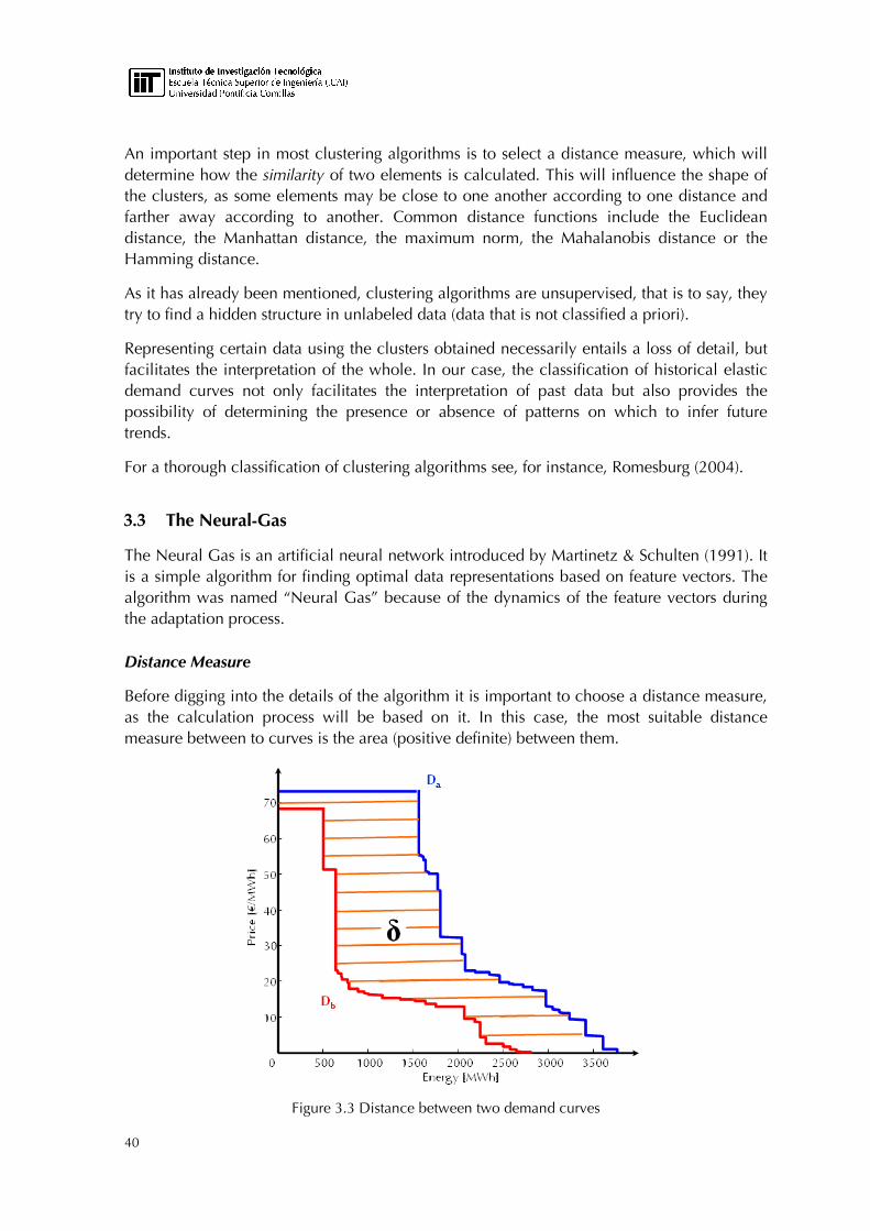
40
An important step in most clustering algorithms is to select a distance measure, which will determine how the similarity of two elements is calculated. This will influence the shape of the clusters, as some elements may be close to one another according to one distance and farther away according to another. Common distance functions include the Euclidean distance, the Manhattan distance, the maximum norm, the Mahalanobis distance or the Hamming distance.
As it has already been mentioned, clustering algorithms are unsupervised, that is to say, they try to find a hidden structure in unlabeled data (data that is not classified a priori).
Representing certain data using the clusters obtained necessarily entails a loss of detail, but facilitates the interpretation of the whole. In our case, the classification of historical elastic demand curves not only facilitates the interpretation of past data but also provides the possibility of determining the presence or absence of patterns on which to infer future trends.
For a thorough classification of clustering algorithms see, for instance, Romesburg (2004).
3.3 The Neural-Gas
The Neural Gas is an artificial neural network introduced by Martinetz & Schulten (1991). It is a simple algorithm for finding optimal data representations based on feature vectors. The algorithm was named “Neural Gas” because of the dynamics of the feature vectors during the adaptation process.
Distance Measure
Before digging into the details of the algorithm it is important to choose a distance measure, as the calculation process will be based on it. In this case, the most suitable distance measure between to curves is the area (positive definite) between them.
Figure 3.3 Distance between two demand curves
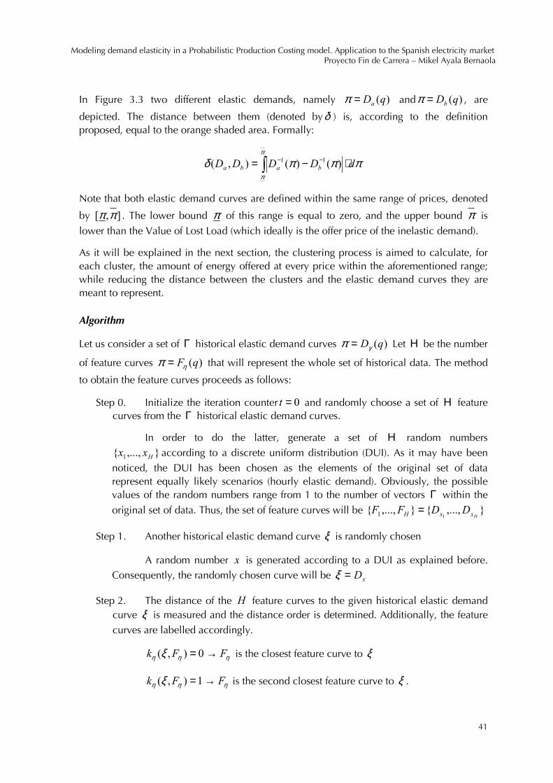
Modeling demand elasticity in a Probabilistic Production Costing model. Application to the Spanish electricity market Proyecto Fin de Carrera – Mikel Ayala Bernaola
41
In Figure 3.3 two different elastic demands, namely )(qDa=π and )(qDb=π , are
depicted. The distance between them (denoted byδ ) is, according to the definition proposed, equal to the orange shaded area. Formally:
πππδπ
π
dDDDD baba ⋅−= ∫−− )()(),( 11
Note that both elastic demand curves are defined within the same range of prices, denoted
by ],[ ππ . The lower bound π of this range is equal to zero, and the upper bound π is
lower than the Value of Lost Load (which ideally is the offer price of the inelastic demand).
As it will be explained in the next section, the clustering process is aimed to calculate, for each cluster, the amount of energy offered at every price within the aforementioned range; while reducing the distance between the clusters and the elastic demand curves they are meant to represent.
Algorithm
Let us consider a set of Γ historical elastic demand curves )(qDγπ = Let Η be the number
of feature curves )(qFηπ = that will represent the whole set of historical data. The method
to obtain the feature curves proceeds as follows:
Step 0. Initialize the iteration counter 0=t and randomly choose a set of Η feature curves from the Γ historical elastic demand curves.
In order to do the latter, generate a set of Η random numbers
,..., 1 Hxx according to a discrete uniform distribution (DUI). As it may have been
noticed, the DUI has been chosen as the elements of the original set of data represent equally likely scenarios (hourly elastic demand). Obviously, the possible values of the random numbers range from 1 to the number of vectors Γ within the
original set of data. Thus, the set of feature curves will be ,...,,...,11 HxxH DDFF =
Step 1. Another historical elastic demand curve ξ is randomly chosen
A random number x is generated according to a DUI as explained before. Consequently, the randomly chosen curve will be xD=ξ
Step 2. The distance of the H feature curves to the given historical elastic demand curve ξ is measured and the distance order is determined. Additionally, the feature
curves are labelled accordingly.
ηηη ξ FFk →= 0),( is the closest feature curve to ξ
ηηη ξ FFk →=1),( is the second closest feature curve to ξ .
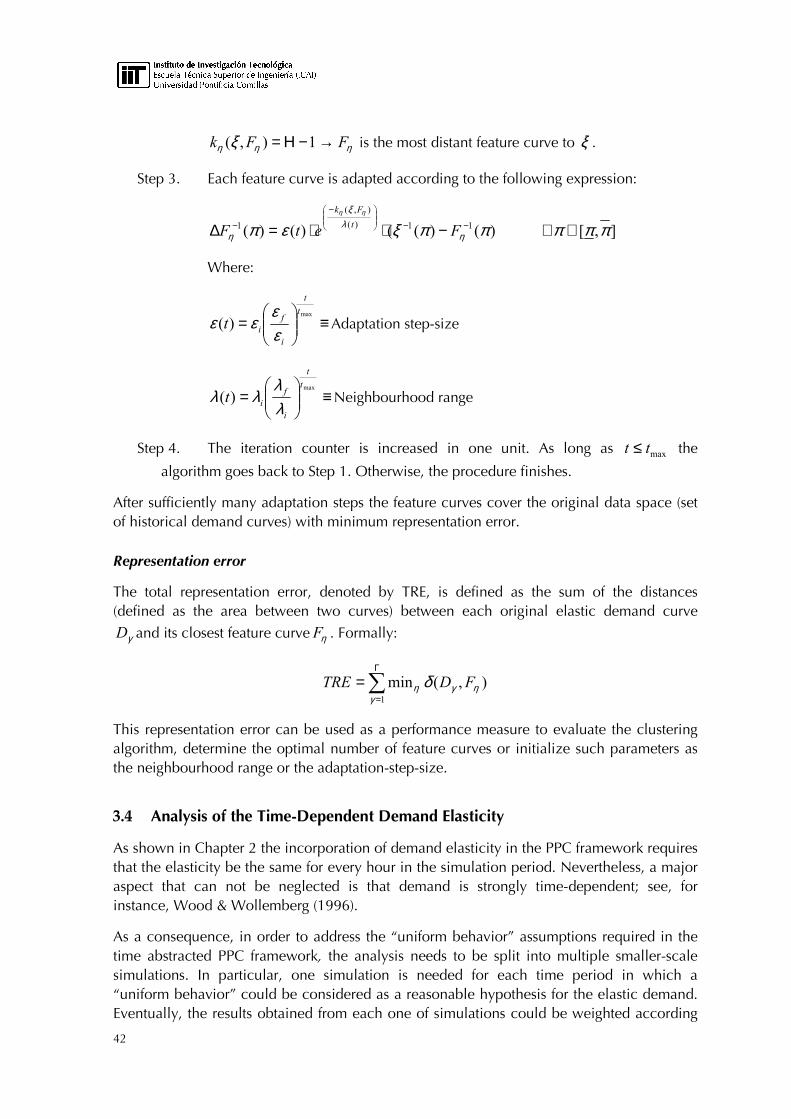
42
ηηη ξ FFk →−Η= 1),( is the most distant feature curve to ξ .
Step 3. Each feature curve is adapted according to the following expression:
)()(()()( 11)(
),(
1 ππξεπ ηλ
ξ
η
ηη
−−
−
− −⋅⋅=∆ FetFt
Fk
],[ πππ ∈∀
Where:
≡
=
max
)(t
t
i
f
itεε
εε Adaptation step-size
≡
=
max
)(t
t
i
f
itλλ
λλ Neighbourhood range
Step 4. The iteration counter is increased in one unit. As long as maxtt ≤ the
algorithm goes back to Step 1. Otherwise, the procedure finishes.
After sufficiently many adaptation steps the feature curves cover the original data space (set of historical demand curves) with minimum representation error.
Representation error
The total representation error, denoted by TRE, is defined as the sum of the distances (defined as the area between two curves) between each original elastic demand curve
γD and its closest feature curve ηF . Formally:
∑Γ
=
=1
),(minγ
ηγη δ FDTRE
This representation error can be used as a performance measure to evaluate the clustering algorithm, determine the optimal number of feature curves or initialize such parameters as the neighbourhood range or the adaptation-step-size.
3.4 Analysis of the Time-Dependent Demand Elasticity
As shown in Chapter 2 the incorporation of demand elasticity in the PPC framework requires that the elasticity be the same for every hour in the simulation period. Nevertheless, a major aspect that can not be neglected is that demand is strongly time-dependent; see, for instance, Wood & Wollemberg (1996).
As a consequence, in order to address the “uniform behavior” assumptions required in the time abstracted PPC framework, the analysis needs to be split into multiple smaller-scale simulations. In particular, one simulation is needed for each time period in which a “uniform behavior” could be considered as a reasonable hypothesis for the elastic demand. Eventually, the results obtained from each one of simulations could be weighted according

Modeling demand elasticity in a Probabilistic Production Costing model. Application to the Spanish electricity market Proyecto Fin de Carrera – Mikel Ayala Bernaola
43
to the number of hours they represented (i.e. the number of hours of the period in which a uniform behavior of elasticity is assumed).
In this Section we show how the clustering algorithm described in Section 3.3 is used to assess the number of time periods where the “uniform behavior” hypothesis can be considered as a reasonable assumption, how the optimal number of periods is determined and how the time scope of analysis is divided.
3.4.1 Determination of the Optimal Number of Clusters
As pointed out in Sugar & James (2003), the correct choice of the number of clusters is often ambiguous, with interpretations depending on the shape and scale of curves in the original data set and the desired clustering resolution.
However, increasing the number of clusters will tend to reduce the amount of representation error in the resulting clustering, to the extreme case of zero error if each original curve is considered its own cluster.
Intuitively then, the optimal choice of the number of clusters will strike a balance between maximum compression of the data using a single cluster, and maximum accuracy by assigning each data point to its own cluster.
Balancing Accuracy and Simplicity
By means of an example, we will show how to choose qualitatively a set of clusters that is comprehensive enough but not unnecessarily exhaustive. Figure 3.4.1-I shows a set of hourly elastic demand curves (in yellow), and a single cluster (in green) that intends to represent the whole set. As it can be recognized, although the cluster is close to the vast majority of the demand curves, there are some outliers in the left side that greatly differ from the cluster that is supposed to be proxy for them. Hence, using a single cluster in this case is obviously not accurate.
Figure 3.4.1-I Historical demand curves. #1 Cluster
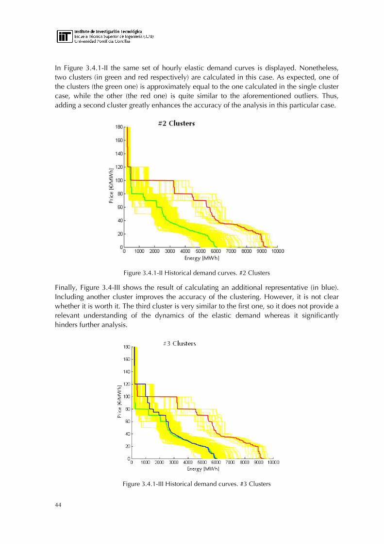
44
In Figure 3.4.1-II the same set of hourly elastic demand curves is displayed. Nonetheless, two clusters (in green and red respectively) are calculated in this case. As expected, one of the clusters (the green one) is approximately equal to the one calculated in the single cluster case, while the other (the red one) is quite similar to the aforementioned outliers. Thus, adding a second cluster greatly enhances the accuracy of the analysis in this particular case.
Figure 3.4.1-II Historical demand curves. #2 Clusters
Finally, Figure 3.4-III shows the result of calculating an additional representative (in blue). Including another cluster improves the accuracy of the clustering. However, it is not clear whether it is worth it. The third cluster is very similar to the first one, so it does not provide a relevant understanding of the dynamics of the elastic demand whereas it significantly hinders further analysis.
Figure 3.4.1-III Historical demand curves. #3 Clusters

Modeling demand elasticity in a Probabilistic Production Costing model. Application to the Spanish electricity market Proyecto Fin de Carrera – Mikel Ayala Bernaola
45
We can therefore conclude that the two-cluster approach is (qualitatively) the one that better combines both accuracy and simplicity.
The Elbow method
The analytical method used to deciding on the number of clusters is the so-called Elbow method, see Long et. al (2010). It looks at the total representation error as defined in Section 3.3 and is founded upon a rather intuitive idea: The number of clusters should be chosen so that adding another cluster does not give much better modelling of the data.
More precisely, if the total representation error is plotted against the number of clusters, the first clusters will add much information (reduce notably the error), but at some point the marginal gain will drop, giving an angle in the plot. The number of clusters is chosen at this point, hence the "elbow criterion"
The marginal reduction of the Total Representation Error is intuitively defined as follows:
1#
#1##
−
− −=∆Clusters
ClustersClustersClusters
TRE
TRETRETRE
Chart 3.4.1 shows the Total Representation Error (and its marginal reduction) committed when using different number of clusters to represent a given set of hourly curves (the hourly curves a whole month).
Chart 3.4.1 Total Representation Error
As it can be observed in the chart and even more clearly in Figure 3.4.1-IV, the marginal reduction of the error drops dramatically beyond two clusters. Thus, there is no sense in further complicating the analysis and two clusters should be chosen in this case.
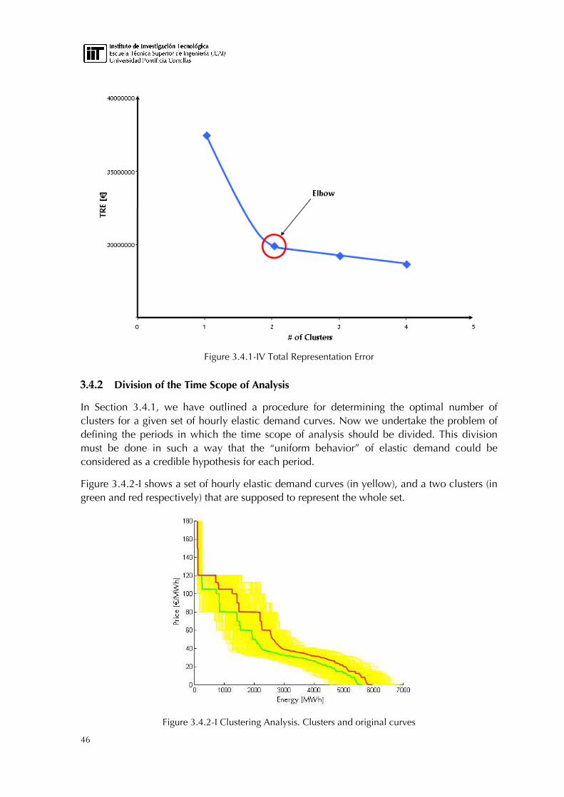
46
Figure 3.4.1-IV Total Representation Error
3.4.2 Division of the Time Scope of Analysis
In Section 3.4.1, we have outlined a procedure for determining the optimal number of clusters for a given set of hourly elastic demand curves. Now we undertake the problem of defining the periods in which the time scope of analysis should be divided. This division must be done in such a way that the “uniform behavior” of elastic demand could be considered as a credible hypothesis for each period.
Figure 3.4.2-I shows a set of hourly elastic demand curves (in yellow), and a two clusters (in green and red respectively) that are supposed to represent the whole set.
Figure 3.4.2-I Clustering Analysis. Clusters and original curves
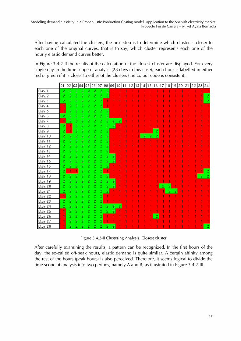
Modeling demand elasticity in a Probabilistic Production Costing model. Application to the Spanish electricity market Proyecto Fin de Carrera – Mikel Ayala Bernaola
47
After having calculated the clusters, the next step is to determine which cluster is closer to each one of the original curves, that is to say, which cluster represents each one of the hourly elastic demand curves better.
In Figure 3.4.2-II the results of the calculation of the closest cluster are displayed. For every single day in the time scope of analysis (28 days in this case), each hour is labelled in either red or green if it is closer to either of the clusters (the colour code is consistent).
Figure 3.4.2-II Clustering Analysis. Closest cluster
After carefully examining the results, a pattern can be recognized. In the first hours of the day, the so-called off-peak hours, elastic demand is quite similar. A certain affinity among the rest of the hours (peak hours) is also perceived. Therefore, it seems logical to divide the time scope of analysis into two periods, namely A and B, as illustrated in Figure 3.4.2-III.
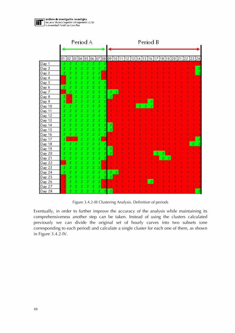
48
Figure 3.4.2-III Clustering Analysis. Definition of periods
Eventually, in order to further improve the accuracy of the analysis while maintaining its comprehensiveness another step can be taken. Instead of using the clusters calculated previously we can divide the original set of hourly curves into two subsets (one corresponding to each period) and calculate a single cluster for each one of them, as shown in Figure 3.4.2-IV.
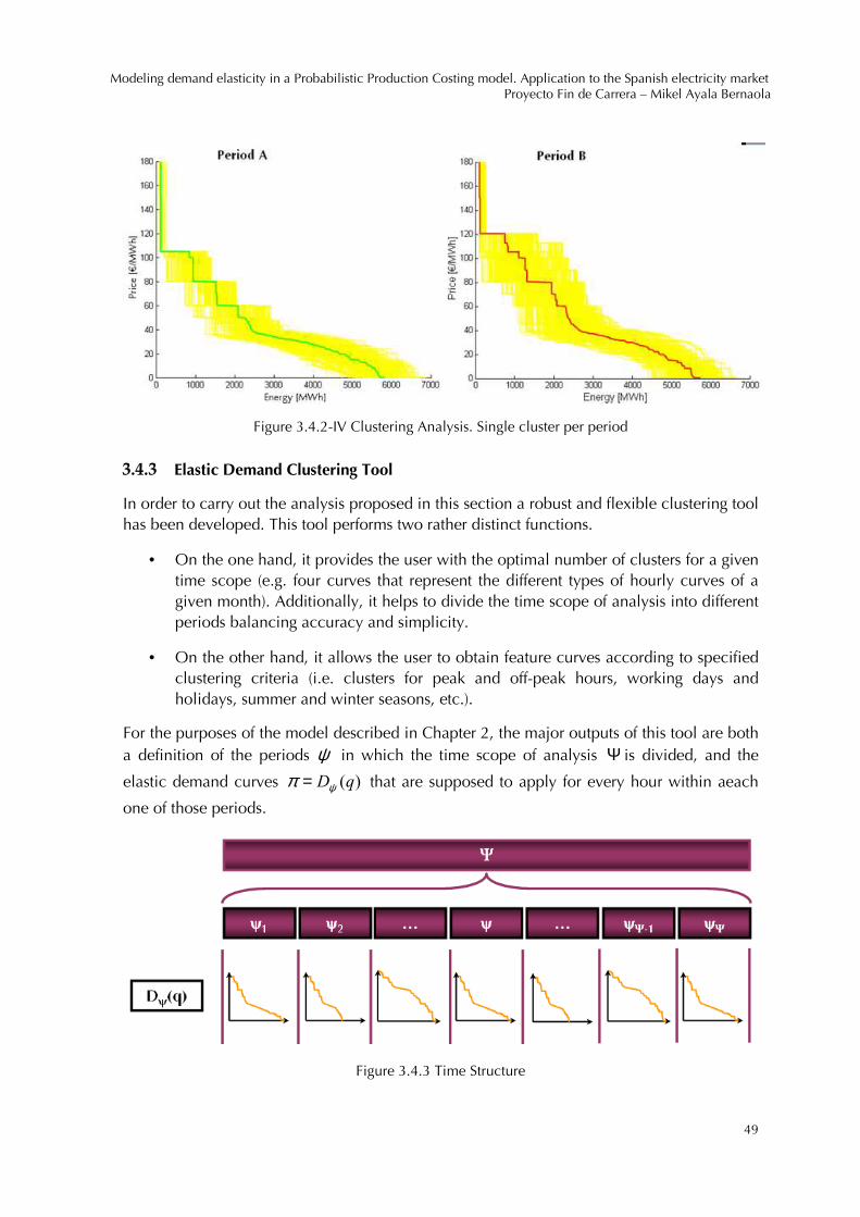
Modeling demand elasticity in a Probabilistic Production Costing model. Application to the Spanish electricity market Proyecto Fin de Carrera – Mikel Ayala Bernaola
49
Figure 3.4.2-IV Clustering Analysis. Single cluster per period
3.4.3 Elastic Demand Clustering Tool
In order to carry out the analysis proposed in this section a robust and flexible clustering tool has been developed. This tool performs two rather distinct functions.
• On the one hand, it provides the user with the optimal number of clusters for a given time scope (e.g. four curves that represent the different types of hourly curves of a given month). Additionally, it helps to divide the time scope of analysis into different periods balancing accuracy and simplicity.
• On the other hand, it allows the user to obtain feature curves according to specified clustering criteria (i.e. clusters for peak and off-peak hours, working days and holidays, summer and winter seasons, etc.).
For the purposes of the model described in Chapter 2, the major outputs of this tool are both a definition of the periods ψ in which the time scope of analysis Ψ is divided, and the
elastic demand curves )(qDψπ = that are supposed to apply for every hour within aeach
one of those periods.
Figure 3.4.3 Time Structure

50
3.5 Conclusions
In this Chapter, the challenge of developing a tool that captures the time-dependent nature of elastic demand has been met. The tool proposed allows for finding patterns and obtaining clusters to realistically describe the elastic demand while avoiding the inconvenience of taking into account too many hourly demand curves.
This clustering tool will be used in Chapter 4 to characterize the elastic demand of the Spanish electricity market. That is to say, it will be used to determine how many different elastic demand scenarios are necessary to fairly represent the whole Spanish elastic consumption.
3.6 References
Aldenderfer, M.S. & R.K. Blashfield (1984). “Cluster Analysis”. Sage Publications, Newbury Park (CA), 1984.
Long, B., Z. Zhang & P.S. Yu (2010). “Relational Data Clustering. Models, Algorithms and Applications, 1st Edition”. Chapman and Hall, CRC Data Mining and Knowledge Discovery Series, 2010.
Martinetz, T. & K. Schulten (1991). “A Neural Gas Network Learns Topologies”. Artificial Neural Networks, Elsevier Science Publishers, pp. 397-402, 1991.
Romesburg, H.C. (2004). “Cluster Analysis for Researchers”. Lulu Press, North Carolina, 2004.
Sugar, C. A. & G. M. James (2003). "Finding the number of clusters in a data set: An information theoretic approach". Journal of the American Statistical Association 98, pp. 750–763, January 2003
Wood, A.J. & B.F. Wollemberg (1996). “Power Generation, Operation and Control”. , 1996

Modeling demand elasticity in a Probabilistic Production Costing model. Application to the Spanish electricity market Proyecto Fin de Carrera – Mikel Ayala Bernaola
51
4. CASE EXAMPLE: APPLICATION TO THE SPANISH ELECTRICITY MARKET
4.1 Introduction
In Chapter 2 we formulated a Probabilistic Production Costing model to estimate the reliability of a power generation system. The model proposed is particularly suited for carrying out reliability assessments in electricity markets where elastic demand consumption is substantial. Notwithstanding, the model is also able to cope with a wide variety of peculiarities that arise in electricity wholesale markets.
Additionally, in Chapter 3, we developed a tool that captures the time-dependent nature of demand elasticity. The tool produced allows for finding patterns and obtaining clusters to realistically describe the elastic demand of a given electricity market.
In this Chapter, we proceed to face the analysis of a real-size electricity market. We will test the capabilities of the models described in this dissertation by carrying out a simulation of the Spanish electricity market for 2016. In this context, we will put a strong emphasis on taking into consideration demand elasticity. Furthermore, we will thoroughly evaluate how traditional reliability measures (as, for instance, the Loss of Load Probability or Expected Non-Served Energy) are affected when such non-negligible demand elasticity is considered.
4.1.1 Structure of the Chapter
The Chapter proceeds as follows. In Section 4.2 we describe the characteristics of the Spanish electricity market that is going to be analysed, the assumptions made and the data that is going to be used as an input for the PPC model. Section 4.3 presents the structure of the simulation. Section 4.4 reviews and discusses the results obtained. Section 4.5 concludes and comments some applications and extensions.
4.2 The Spanish Electricity System
This section is devoted to describe the way the Spanish electricity market has been modelled. The structure of the section mirrors that of Chapter 2. In this case however, instead of modelling each one of the elements of the power system within the PPC framework we present the data that is going to be used in the simulation, along with the assumptions and projections made.
4.2.1 Load Scenario
In order to obtain the hourly values of load that are going to be used as an input to the PPC model as described in Section 2.3.1 we take, as a starting point, the chronological load profile from 2009. This hourly load profile is scaled up according to an estimation of demand growth as depicted in Figure 4.2.1.
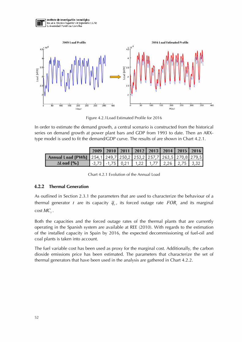
52
Figure 4.2.1Load Estimated Profile for 2016
In order to estimate the demand growth, a central scenario is constructed from the historical series on demand growth at power plant bars and GDP from 1993 to date. Then an ARX-type model is used to fit the demand/GDP curve. The results of are shown in Chart 4.2.1.
Chart 4.2.1 Evolution of the Annual Load
4.2.2 Thermal Generation
As outlined in Section 2.3.1 the parameters that are used to characterize the behaviour of a
thermal generator t are its capacity tq , its forced outage rate tFOR and its marginal
cost tMC .
Both the capacities and the forced outage rates of the thermal plants that are currently operating in the Spanish system are available at REE (2010). With regards to the estimation of the installed capacity in Spain by 2016, the expected decommissioning of fuel-oil and coal plants is taken into account.
The fuel variable cost has been used as proxy for the marginal cost. Additionally, the carbon dioxide emissions price has been estimated. The parameters that characterize the set of thermal generators that have been used in the analysis are gathered in Chart 4.2.2.

Modeling demand elasticity in a Probabilistic Production Costing model. Application to the Spanish electricity market Proyecto Fin de Carrera – Mikel Ayala Bernaola
53
Chart 4.2.2 Thermal Generation Data
Figure 4.2.2 shows the implied supply function when every single generator is available.
Figure 4.2.2 Thermal generation supply curve
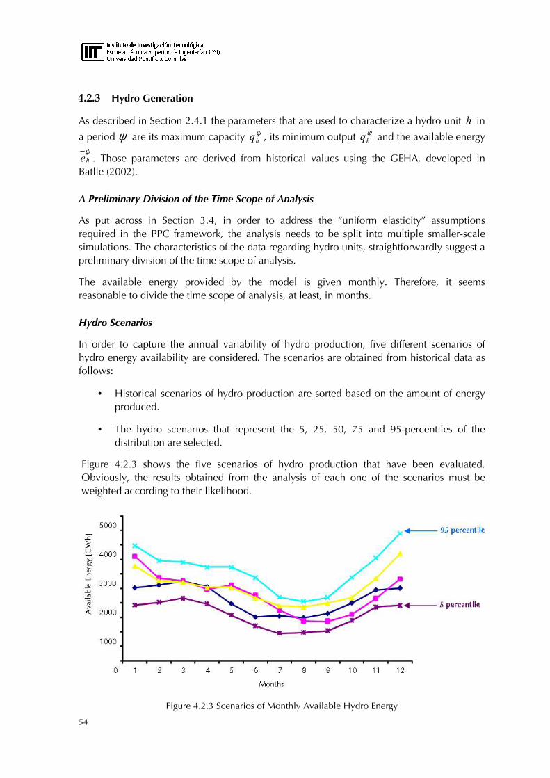
54
4.2.3 Hydro Generation
As described in Section 2.4.1 the parameters that are used to characterize a hydro unit h in
a period ψ are its maximum capacity ψhq , its minimum output ψ
hq and the available energy ψhe . Those parameters are derived from historical values using the GEHA, developed in
Batlle (2002).
A Preliminary Division of the Time Scope of Analysis
As put across in Section 3.4, in order to address the “uniform elasticity” assumptions required in the PPC framework, the analysis needs to be split into multiple smaller-scale simulations. The characteristics of the data regarding hydro units, straightforwardly suggest a preliminary division of the time scope of analysis.
The available energy provided by the model is given monthly. Therefore, it seems reasonable to divide the time scope of analysis, at least, in months.
Hydro Scenarios
In order to capture the annual variability of hydro production, five different scenarios of hydro energy availability are considered. The scenarios are obtained from historical data as follows:
• Historical scenarios of hydro production are sorted based on the amount of energy produced.
• The hydro scenarios that represent the 5, 25, 50, 75 and 95-percentiles of the distribution are selected.
Figure 4.2.3 shows the five scenarios of hydro production that have been evaluated. Obviously, the results obtained from the analysis of each one of the scenarios must be weighted according to their likelihood.
Figure 4.2.3 Scenarios of Monthly Available Hydro Energy

Modeling demand elasticity in a Probabilistic Production Costing model. Application to the Spanish electricity market Proyecto Fin de Carrera – Mikel Ayala Bernaola
55
4.2.4 RES Generation
In order to obtain the hourly values of production of Renewable Energy Sources that are going to be used as an input to the PPC model as described in Section 2.5 we take, as a starting point, the chronological production profile from 2009.This hourly production profile is scaled up in consonance with the estimated RES production increase for 2016 based on governmental planning (that is to say, ~40%) as shown in Figure 4.2.4.
Figure 4.2.4 RES Generation Estimated Profile for 2016
4.2.5 Elastic Demand
In this case example we consider two different sources of demand elasticity: On the one hand, the elasticity reflected and extracted from the bids made by participants in the Spanish power pool in the past years and, on the other hand, the interruptible load bilaterally contracted by the Transmission System Operator to the largest industrial consumers in the system.
Demand Bids from Market Participants. Price-Sensitive Demand
We have taken into account the bids made hourly by market participants in the day-ahead Spanish electricity market along 2010.
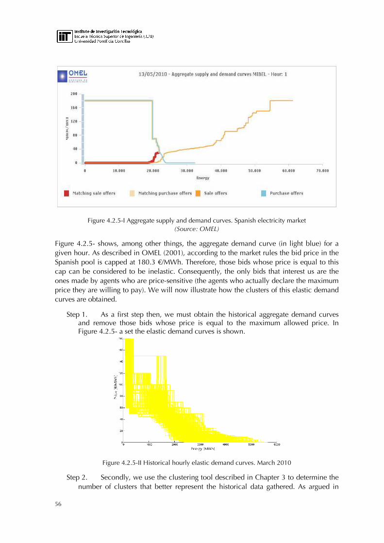
56
Figure 4.2.5-I Aggregate supply and demand curves. Spanish electricity market (Source: OMEL)
Figure 4.2.5- shows, among other things, the aggregate demand curve (in light blue) for a given hour. As described in OMEL (2001), according to the market rules the bid price in the Spanish pool is capped at 180.3 €/MWh. Therefore, those bids whose price is equal to this cap can be considered to be inelastic. Consequently, the only bids that interest us are the ones made by agents who are price-sensitive (the agents who actually declare the maximum price they are willing to pay). We will now illustrate how the clusters of this elastic demand curves are obtained.
Step 1. As a first step then, we must obtain the historical aggregate demand curves and remove those bids whose price is equal to the maximum allowed price. In Figure 4.2.5- a set the elastic demand curves is shown.
Figure 4.2.5-II Historical hourly elastic demand curves. March 2010
Step 2. Secondly, we use the clustering tool described in Chapter 3 to determine the number of clusters that better represent the historical data gathered. As argued in

Modeling demand elasticity in a Probabilistic Production Costing model. Application to the Spanish electricity market Proyecto Fin de Carrera – Mikel Ayala Bernaola
57
Section 4.2.3, the time scope of analysis will, at least, be divided in months. Accordingly, the clustering process will aim to determine the optimal number of clusters for each month.
Figure 4.2.5-III illustrates the result of calculating different numbers of clusters for the data presented in Figure 4.2.5-II Historical hourly elastic demand curves. March 2010.
Figure 4.2.5-I Different number of clusters. March 2011
As explained in Section 3.4.1, in order to determine the optimal number of clusters the total representation error committed has to be measured. Chart 4.2.5 shows the marginal reduction of the total representation error committed when using different numbers of clusters to represent the hourly curves of each month.

58
Chart 4.2.5 Marginal reduction of the representation error
As it can be noticed, the marginal reduction of the error does not decrease significantly when adding a third or a fourth cluster. Therefore, it does not make sense to further complicate the analysis and two clusters per month will be calculated. This decision is reinforced by merely having a look at Figure 4.2.5-III, in which the average Total Representation Error committed per month is depicted. The so-called “elbow” (see Section 3.4.1) is clearly in the neighbourhood of the point that represents the error committed when using two clusters.
Figure 4.2.5-III Average representation error per month
Step 3. Finally, the time scope of analysis must be divided appropriately. Each month will be split into two periods. In order to define those periods, we must calculate
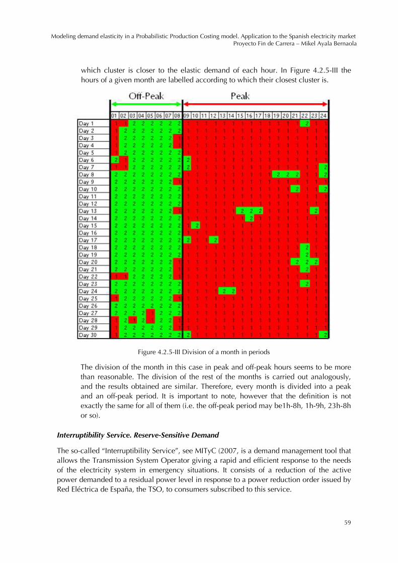
Modeling demand elasticity in a Probabilistic Production Costing model. Application to the Spanish electricity market Proyecto Fin de Carrera – Mikel Ayala Bernaola
59
which cluster is closer to the elastic demand of each hour. In Figure 4.2.5-III the hours of a given month are labelled according to which their closest cluster is.
Figure 4.2.5-III Division of a month in periods
The division of the month in this case in peak and off-peak hours seems to be more than reasonable. The division of the rest of the months is carried out analogously, and the results obtained are similar. Therefore, every month is divided into a peak and an off-peak period. It is important to note, however that the definition is not exactly the same for all of them (i.e. the off-peak period may be1h-8h, 1h-9h, 23h-8h or so).
Interruptibility Service. Reserve-Sensitive Demand
The so-called “Interruptibility Service”, see MITyC (2007, is a demand management tool that allows the Transmission System Operator giving a rapid and efficient response to the needs of the electricity system in emergency situations. It consists of a reduction of the active power demanded to a residual power level in response to a power reduction order issued by Red Eléctrica de España, the TSO, to consumers subscribed to this service.
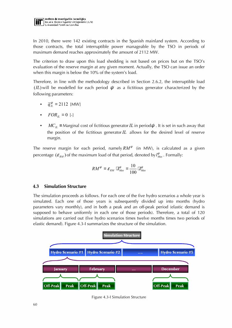
60
In 2010, there were 142 existing contracts in the Spanish mainland system. According to those contracts, the total interruptible power manageable by the TSO in periods of maximum demand reaches approximately the amount of 2112 MW.
The criterion to draw upon this load shedding is not based on prices but on the TSO’s evaluation of the reserve margin at any given moment. Actually, the TSO can issue an order when this margin is below the 10% of the system’s load.
Therefore, in line with the methodology described in Section 2.6.2, the interruptible load )(IL will be modelled for each period ψ as a fictitious generator characterized by the
following parameters:
• 2112=ψILq [MW]
• 0=ILFOR [-]
• ≡ILMC Marginal cost of fictitious generator IL in periodψ . It is set in such away that
the position of the fictitious generator IL allows for the desired level of reserve margin.
The reserve margin for each period, namely ψRM (in MW), is calculated as a given
percentage )( RMε of the maximum load of that period, denoted by ψMaxl . Formally:
ψψψ ε MaxMaxRM llRM ⋅=⋅=100
10
4.3 Simulation Structure
The simulation proceeds as follows. For each one of the five hydro scenarios a whole year is simulated. Each one of those years is subsequently divided up into months (hydro parameters vary monthly), and in both a peak and an off-peak period (elastic demand is supposed to behave uniformly in each one of those periods). Therefore, a total of 120 simulations are carried out (five hydro scenarios times twelve months times two periods of elastic demand). Figure 4.3-I summarizes the structure of the simulation.
Figure 4.3-I Simulation Structure
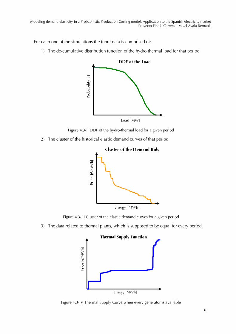
Modeling demand elasticity in a Probabilistic Production Costing model. Application to the Spanish electricity market Proyecto Fin de Carrera – Mikel Ayala Bernaola
61
For each one of the simulations the input data is comprised of:
1) The de-cumulative distribution function of the hydro thermal load for that period.
Figure 4.3-II DDF of the hydro-thermal load for a given period
2) The cluster of the historical elastic demand curves of that period.
Figure 4.3-III Cluster of the elastic demand curves for a given period
3) The data related to thermal plants, which is supposed to be equal for every period.
Figure 4.3-IV Thermal Supply Curve when every generator is available

62
4) The data related to the interruptible load, which is supposed to be equal for every period as well.
5) And the data related to hydro units. The disaggregation presented (by peak and off-peak hours) allows us to better represent the dispatch of hydro plants. The manageable production (which was termed as available energy over minimum in Section 2.3.1) is only used in peak hours while the run-of-the-river output is kept both in peak and off-peak hours.
Figure 4.3-V shows the equivalent supply curve for a given period. This curve is built upon the modeling assumptions described in Chapter 2. As it can be noted, elastic demand bids are modeled as equivalent thermal generators; hydro generation is split into the run-of-the-river output (offered at zero price) and the manageable production and the interruptible load is modeled as an equivalent generator that allows for a certain reserve margin.
Figure 4.3-V Equivalent Supply Curve for a given period
4.4 Case Example Results
In order to illustrate the discussion regarding the need for new reliability measures presented in Chapter 1, we ran two simulations:
• “Active Role of Demand” scenario. In this simulation demand elasticity was taken into account as described in Section 4.2.
• “Business As Usual” scenario. In this case, demand elasticity is neglected and all the load is supposed to be inelastic (as in conventional PPC models)
Figure 4.4-I shows the result of the probabilistic loading for a given period when demand elasticity is taken into consideration.

Modeling demand elasticity in a Probabilistic Production Costing model. Application to the Spanish electricity market Proyecto Fin de Carrera – Mikel Ayala Bernaola
63
Figure 4.4-I Successive Equivalent Load Curves. Active Role of Demand
Figure 4.4-II shows the result of the probabilistic loading for the same period when demand elasticity is left aside.
Figure 4.4-II Successive Equivalent Load Curves. Business As Usual

64
4.4.1 Classical Reliability Measures
We can compare the different values of the traditional reliability measures obtained in the two simulations.
Chart 4.4.1 Classical Reliability Measures. Results
Even in the case of the Spanish electricity system, characterized by a large overcapacity, the magnitude order of the difference is significant. As expected, there is a considerable difference in the values of the LOLP and the ENSE that depends on whether elastic demand is taken into account or not.
As anticipated in Rodilla & Batlle (2009) traditional reliability measures leave aside very meaningful information when used to assess the performance of a system where elastic demand plays an important role. In neither of the scenarios evaluated the information provided by those metrics is fully comprehensive, as they do not capture the total value of the bids that were not accepted.
In the case of the “Active Role of Demand” scenario, this value may be exorbitant but it would lie hidden behind a ridiculously low LOLP that only takes into account the fully inelastic demand. Alternatively, in the case of the “Business As Usual” scenario, the total value of the bids that were not accepted may be negligible but this fact would be concealed by a high LOLP that would lead to think that the system does not meet the minimum reliability requirements.
4.4.2 Value of Non-Purchased Energy
In order to attain a better understanding of the reliability of the system we evaluate the distribution function of the Value of Non-Purchased Energy (see Section 2.7). Figure 4.4.2 shows the distribution function calculated in the “Active Role of Demand” scenario (obviously, it does not make sense to evaluate it in the “Business As Usual” scenario as demand is assumed to be inelastic).
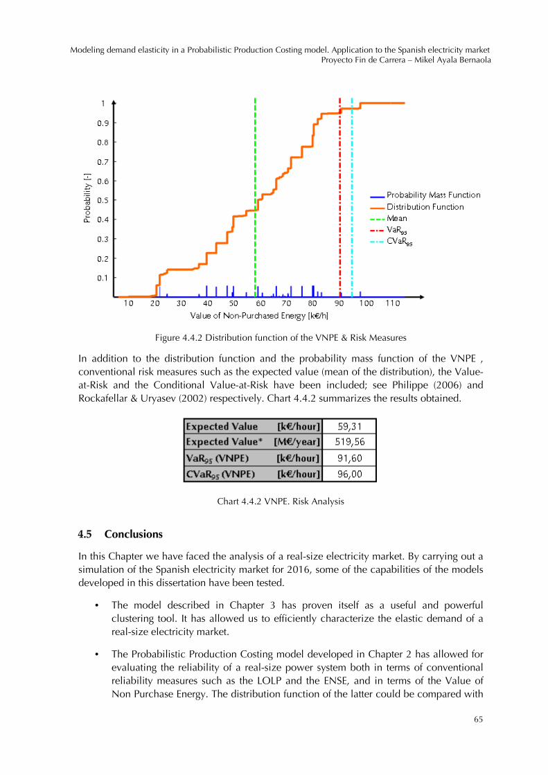
Modeling demand elasticity in a Probabilistic Production Costing model. Application to the Spanish electricity market Proyecto Fin de Carrera – Mikel Ayala Bernaola
65
Figure 4.4.2 Distribution function of the VNPE & Risk Measures
In addition to the distribution function and the probability mass function of the VNPE , conventional risk measures such as the expected value (mean of the distribution), the Value-at-Risk and the Conditional Value-at-Risk have been included; see Philippe (2006) and Rockafellar & Uryasev (2002) respectively. Chart 4.4.2 summarizes the results obtained.
Chart 4.4.2 VNPE. Risk Analysis
4.5 Conclusions
In this Chapter we have faced the analysis of a real-size electricity market. By carrying out a simulation of the Spanish electricity market for 2016, some of the capabilities of the models developed in this dissertation have been tested.
• The model described in Chapter 3 has proven itself as a useful and powerful clustering tool. It has allowed us to efficiently characterize the elastic demand of a real-size electricity market.
• The Probabilistic Production Costing model developed in Chapter 2 has allowed for evaluating the reliability of a real-size power system both in terms of conventional reliability measures such as the LOLP and the ENSE, and in terms of the Value of Non Purchase Energy. The distribution function of the latter could be compared with
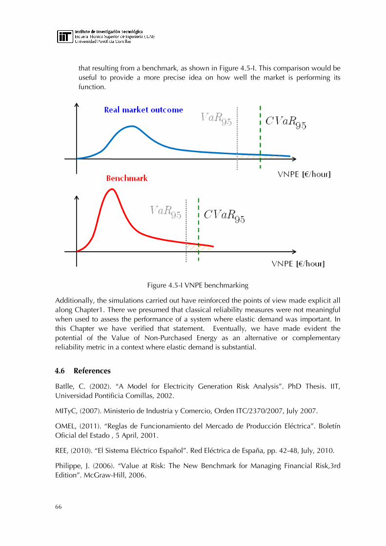
66
that resulting from a benchmark, as shown in Figure 4.5-I. This comparison would be useful to provide a more precise idea on how well the market is performing its function.
Figure 4.5-I VNPE benchmarking
Additionally, the simulations carried out have reinforced the points of view made explicit all along Chapter1. There we presumed that classical reliability measures were not meaningful when used to assess the performance of a system where elastic demand was important. In this Chapter we have verified that statement. Eventually, we have made evident the potential of the Value of Non-Purchased Energy as an alternative or complementary reliability metric in a context where elastic demand is substantial.
4.6 References
Batlle, C. (2002). “A Model for Electricity Generation Risk Analysis”. PhD Thesis. IIT, Universidad Pontificia Comillas, 2002.
MITyC, (2007). Ministerio de Industria y Comercio, Orden ITC/2370/2007, July 2007.
OMEL, (2011). “Reglas de Funcionamiento del Mercado de Producción Eléctrica”. Boletín Oficial del Estado , 5 April, 2001.
REE, (2010). “El Sistema Eléctrico Español”. Red Eléctrica de España, pp. 42-48, July, 2010.
Philippe, J. (2006). “Value at Risk: The New Benchmark for Managing Financial Risk,3rd Edition”. McGraw-Hill, 2006.

Modeling demand elasticity in a Probabilistic Production Costing model. Application to the Spanish electricity market Proyecto Fin de Carrera – Mikel Ayala Bernaola
67
Rockafellar, R.T. & S. Uryasev (2002). “Conditional Value-at-Risk for general loss distributions”. Journal of Banking and Finance, Elsevier, 2002.
Rodilla, P. and C. Batlle (2010). “Redesigning Probabilistic Production Costing Models and Reliability Measures in the Presence of Market Demand Elasticity”. IIT Working Paper IIT-10- 028A, June 2010. Submitted to IEEE Transactions on Power Systems. Available at www.iit.upcomillas.es/batlle.
68
5. CONCLUSIONS
This last chapter is dedicated to evaluating the conclusions that result from the research conducted in this dissertation. It includes a brief summary of the analysis, developments and findings that constitute the core of this work.
5.1 Summary
This dissertation has addressed the problem of developing an adequacy analysis model for electricity markets in which elastic demand plays a significant role. This issue is currently of the most relevance due to the reforms that have been introduced in the power industry worldwide and the upcoming technical and regulatory developments of smart grids and demand response tools that will allow for an increasingly active role of demand.
The following points summarize the analysis carried out and the results obtained in this dissertation.
Development of a PPC model
We have developed a PPC model that is able to cope with a wide variety of peculiarities of electricity wholesale markets. The proposed formulation meets the following modelling challenges:
• Firstly, the model allows for analysis in a conventional thermal generation system with fully inelastic load.
• Secondly, the conventional PPC model has been adapted for loading energy limited units.
• Thirdly, the conventional PPC model has been extended with regard to taking into account intermittent renewable generation.
• Fourthly, an equivalent load and generation model has been constructed to integrate price sensitive demand into the conventional PPC model.
• Fifthly, the PPC model has been adjusted to properly reflect the effect of the reserve-sensitive demand.
• Sixthly, an algorithm to compute the distribution function of the Value of the Non-Purchased Energy has been implemented within the PPC frame-work.
Addressing the Time-Dependent Nature of Demand Elasticity
We have developed as well a methodology that captures the time-dependent nature of demand elasticity. The tool produced allows for finding patterns and obtaining clusters to realistically describe the elastic demand. Additionally, the clustering process is aimed at being comprehensive enough but not unnecessarily exhaustive. The tool performs two rather distinct functions.

Modeling demand elasticity in a Probabilistic Production Costing model. Application to the Spanish electricity market Proyecto Fin de Carrera – Mikel Ayala Bernaola
69
• On the one hand, it provides with the optimal number of clusters for a time scope (e.g. four curves that represent the different types of hourly curves of a given month). Additionally, it helps to divide the time scope of analysis into different periods balancing accuracy and simplicity.
• On the other hand, it allows obtaining feature curves according to specified clustering criteria (i.e. clusters for peak and off-peak hours, working days and holidays, summer and winter seasons, etc.).
Power System Reliability Assessments
Two results regarding reliability assessments of power systems could be highlighted.
• We have verified, in a real-size case example, that traditional reliability measures are not fully comprehensive in a context where elastic demand consumption is substantial.
• We have made evident the potential of the Value of Non-Purchased Energy as a substitute or complementary reliability metric in a context where elastic demand plays an active role. The VNPE could help to reveal a scarcity situation that would otherwise lie hidden behind ridiculously low values of LOLP and ENSE that only take into account the fully inelastic demand.