State and Local Government Expenditures

131 Undergraduate Public Economics

Emmanuel Saez

UC Berkeley

1

FISCAL FEDERALISM

optimal fiscal federalism: The question of which activities

should take place at which level of government

The distribution of government spending has changed dramat-

ically over time in the United States

• Local state and spending have declined considerably.

• Much state and local spending now supported by intergov-

ernmental grants [transfers from the federal government]

2

5 of 35

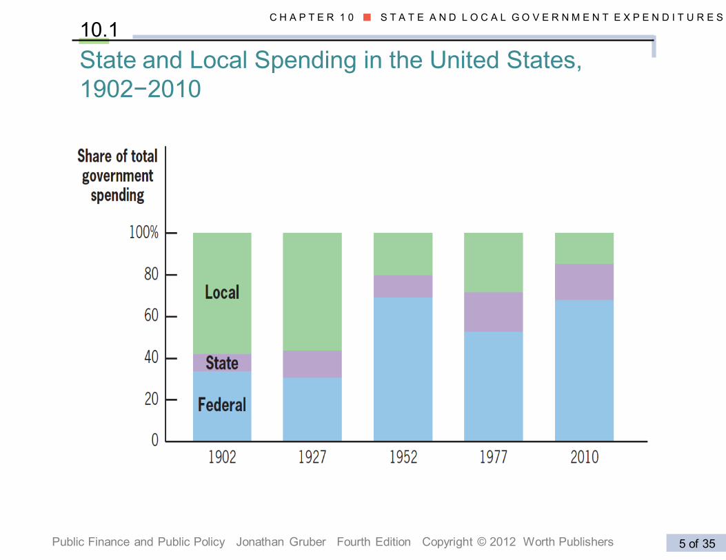
C H A P T E R 1 0 ■ S T A T E A N D L O C A L G O V E R N M E N T E X P E N D I T U R E S

Public Finance and Public Policy Jonathan Gruber Fourth Edition Copyright © 2012 Worth Publishers

10.1

State and Local Spending in the United States,

1902−2010

SPENDING AND REVENUE OF STATE AND

LOCAL GOVERNMENTS

Property tax: The tax on land and any buildings on it, such

as commercial businesses or residential homes.

Main source of revenue from local governments due to:

1) History: real estate property is visible and hence taxable

even in archaic economies with informal businesses

2) Immobile tax base: the real estate tax base cannot flee to

another jurisdiction (mobility of the tax base is an issue for

local governments)

Today, property tax is about 1/3 of revenue raised by state+local

government (rest is 1/3 income tax, 1/3 sales taxes)

4

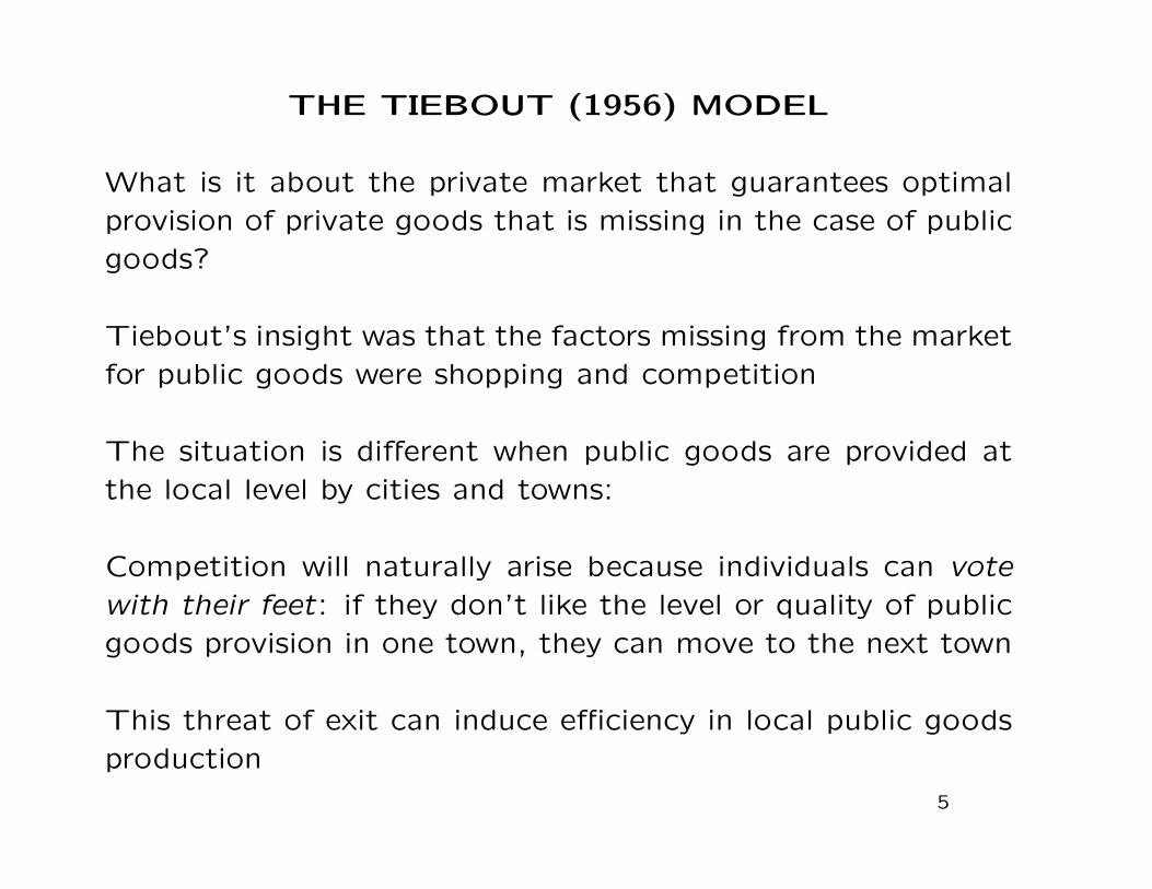
THE TIEBOUT (1956) MODEL

What is it about the private market that guarantees optimalprovision of private goods that is missing in the case of publicgoods?

Tiebout’s insight was that the factors missing from the marketfor public goods were shopping and competition

The situation is different when public goods are provided atthe local level by cities and towns:

Competition will naturally arise because individuals can votewith their feet: if they don’t like the level or quality of publicgoods provision in one town, they can move to the next town

This threat of exit can induce efficiency in local public goodsproduction

5

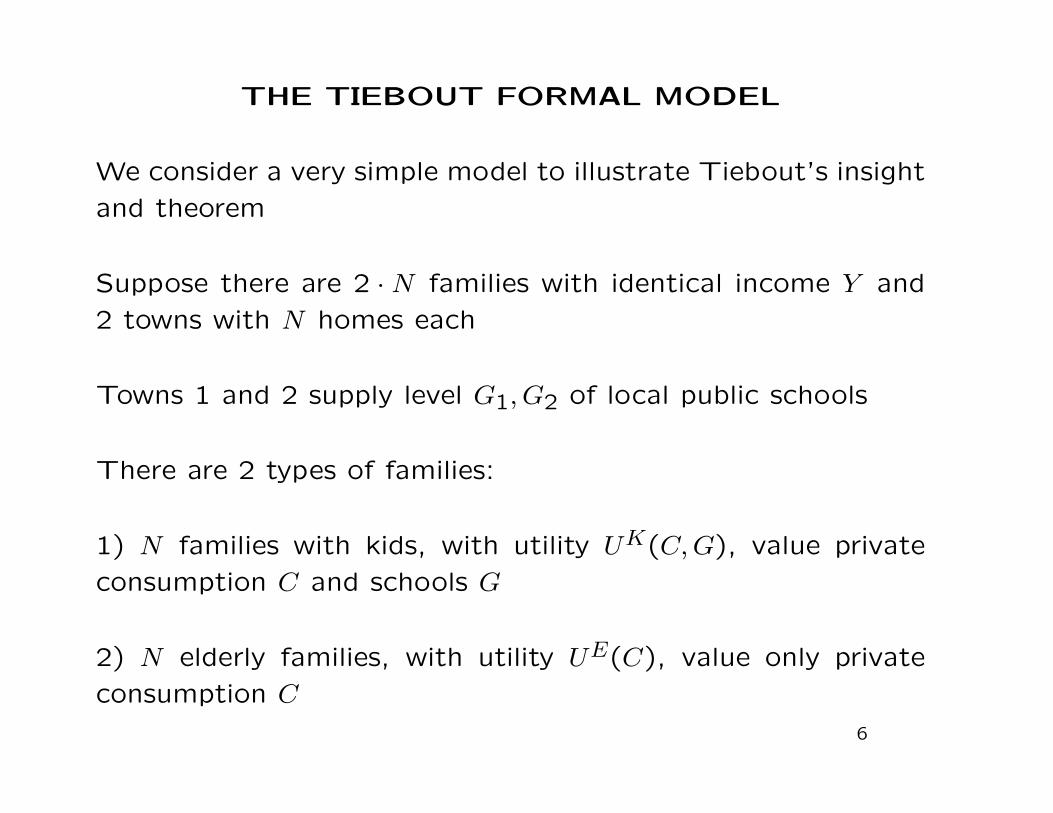
THE TIEBOUT FORMAL MODEL

We consider a very simple model to illustrate Tiebout’s insight

and theorem

Suppose there are 2 · N families with identical income Y and

2 towns with N homes each

Towns 1 and 2 supply level G1, G2 of local public schools

There are 2 types of families:

1) N families with kids, with utility UK(C,G), value private

consumption C and schools G

2) N elderly families, with utility UE(C), value only private

consumption C

6

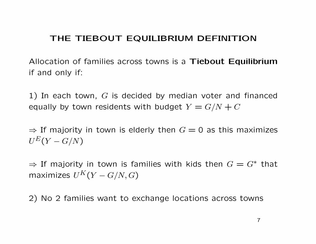
THE TIEBOUT EQUILIBRIUM DEFINITION

Allocation of families across towns is a Tiebout Equilibrium

if and only if:

1) In each town, G is decided by median voter and financed

equally by town residents with budget Y = G/N + C

⇒ If majority in town is elderly then G = 0 as this maximizes

UE(Y −G/N)

⇒ If majority in town is families with kids then G = G∗ that

maximizes UK(Y −G/N,G)

2) No 2 families want to exchange locations across towns

7

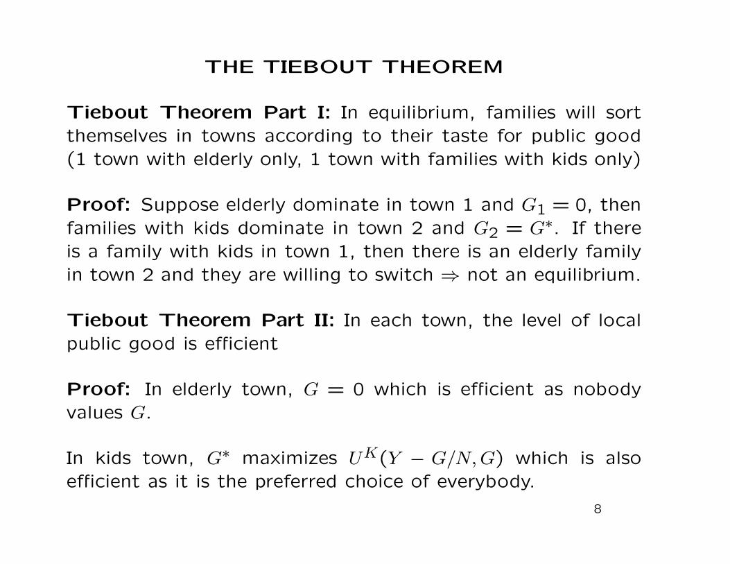
THE TIEBOUT THEOREM

Tiebout Theorem Part I: In equilibrium, families will sortthemselves in towns according to their taste for public good(1 town with elderly only, 1 town with families with kids only)

Proof: Suppose elderly dominate in town 1 and G1 = 0, thenfamilies with kids dominate in town 2 and G2 = G∗. If thereis a family with kids in town 1, then there is an elderly familyin town 2 and they are willing to switch ⇒ not an equilibrium.

Tiebout Theorem Part II: In each town, the level of localpublic good is efficient

Proof: In elderly town, G = 0 which is efficient as nobodyvalues G.

In kids town, G∗ maximizes UK(Y − G/N,G) which is alsoefficient as it is the preferred choice of everybody.

8

THE TIEBOUT MODEL

People can vote with their feet by choosing the locality that

best fits their tastes and provides the best public goods given

the tax

The main message of the model is that competition across

local jurisdictions puts competitive pressure on the provision

of local public goods:

1) Public goods need to reflect tastes of local residents

2) Public goods need to be efficiently provided (without waste)

9

Centralized vs. Decentralized Government

Conservatives/libertarian tend to like decentralized govern-

ments over centralized governments

Conservatives/libertarian dislike redistribution and like individ-

ual choice and competition. In Tiebout model:

1) local governments do not do any redistribution: individuals

receive in local public goods exactly what they are paying in

taxes (= benefit principle of taxation)

2) individuals can choose (through their location choice) their

preferred mix of public goods and taxes

3) competition between local govts forces them to provide

local public good efficiently

10

PROBLEMS WITH THE TIEBOUT MODEL

The Tiebout model is an idealized model that requires a num-ber of assumptions that may not hold perfectly in reality:

1) Individuals can move without any cost across towns

2) Individuals have perfect information on the benefits andtaxes paid in each town

3) There must be enough towns so that individuals can sortthemselves into groups with similar preferences for public goods

4) No externalities/spillovers of public goods across towns[with spillovers across towns, public goods will be under pro-vided in Tiebout model, e.g. parks, police]

5) Local govts can charge “poll” taxes (equal payments perperson) to residents. In reality, local taxes depend on propertyand consumption.

11

EVIDENCE ON THE TIEBOUT MODEL

Tiebout Sorting: Resident Similarity Across Areas

A testable implication of the Tiebout model is that when peo-

ple have more choice of local community, the tastes for public

goods will be more similar among residents than when people

do not have many choices

This fact is indeed pretty well established

More Efficiency when there is more Tiebout sorting

This fact is controversial

12

Evidence on the Tiebout Model: Hoxby (2000)

Hoxby (2000) considers public school districts in the US. Shecompares cities where:

A) There are few large school districts and hence little choicefor residents (such as Miami or LA)

B) There are many small school districts and hence a lot ofchoice for residents (such as Boston)

2 key findings:

I) Cities with few districts have less sorting across neighbor-hood (in terms of school quality) than cities with many dis-tricts (this result is well established)

II) Cities with many districts have higher test scores on aver-age: this result is controversial (see Rothstein, 2007 critique)

13

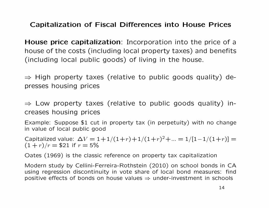
Capitalization of Fiscal Differences into House Prices

House price capitalization: Incorporation into the price of ahouse of the costs (including local property taxes) and benefits(including local public goods) of living in the house.

⇒ High property taxes (relative to public goods quality) de-presses housing prices

⇒ Low property taxes (relative to public goods quality) in-creases housing prices

Example: Suppose $1 cut in property tax (in perpetuity) with no changein value of local public good

Capitalized value: ∆V = 1+1/(1+r)+1/(1+r)2+... = 1/[1−1/(1+r)] =(1 + r)/r = $21 if r = 5%

Oates (1969) is the classic reference on property tax capitalization

Modern study by Cellini-Ferreira-Rothstein (2010) on school bonds in CAusing regression discontinuity in vote share of local bond measures: findpositive effects of bonds on house values ⇒ under-investment in schools

14

240 QUARTERLY JOURNAL OF ECONOMICS

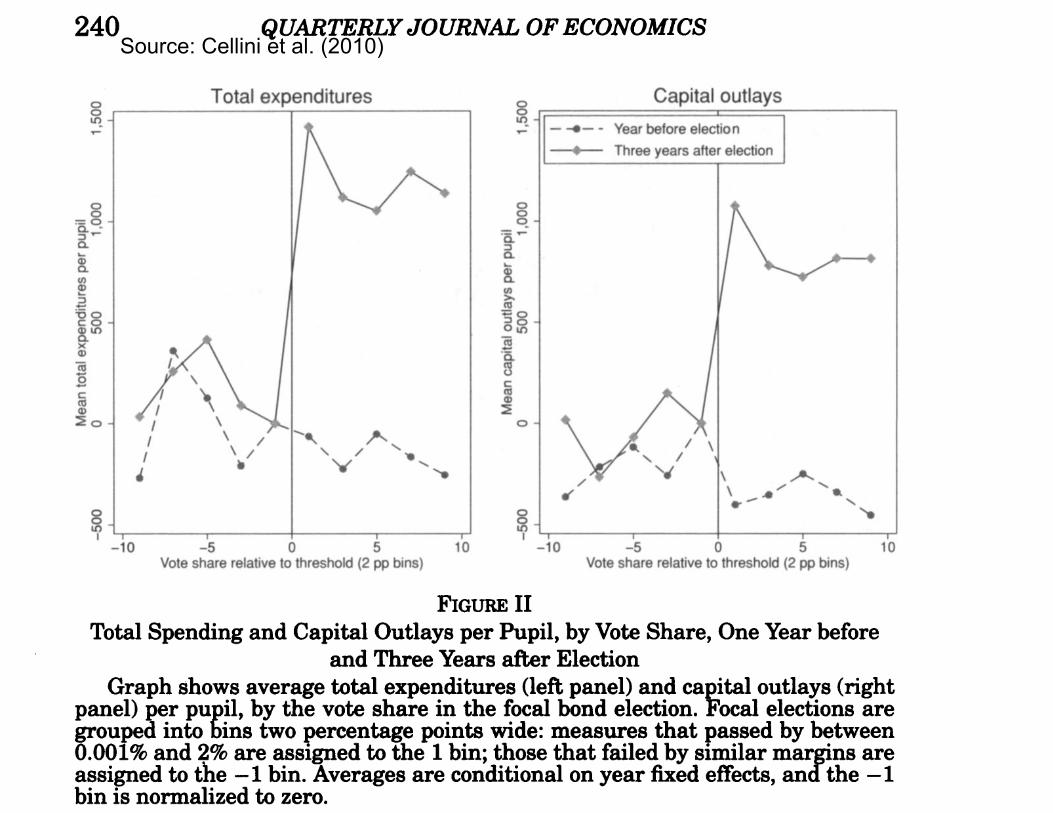
Figure II

Total Spending and Capital Outlays per Pupil, by Vote Share, One Year before and Three Years after Election

Graph shows average total expenditures (left panel) and capital outlays (right panel) per pupil, by the vote share in the focal bond election. Focal elections are grouped into bins two percentage points wide: measures that passed by between 0.001% and 2% are assigned to the 1 bin; those that failed by similar margins are assigned to the -1 bin. Averages are conditional on year fixed effects, and the -1 bin is normalized to zero.

after the election, districts where the measure just passed spend about $1,000 more per pupil, essentially all of it in the capital account.31

Panel A of Table IV presents estimates of the intent-to-treat effect of bond passage on district spending and on state and fed- eral transfers (all in per-pupil terms) over the six years following the election, using equation (7).32 Bond passage has no significant effect on any of the fiscal variables in the first year. We see large increases in capital expenditures in years 2, 3, and 4. These in- creases fade by the fifth year following the election. There is no indication of any effect on current spending in any year, and con- fidence intervals rule out effects amounting to more than about

31. It is possible that districts use bond revenues for operating expenses but report these expenditures in their capital accounts. The CCD data are not used for financial oversight, so districts have no obvious incentive to misreport.

32. We make one modification to equation (7): We constrain the r = 0 coeffi- cients to zero. It is not plausible that bond passage can have effects on that year's district budget, which will typically have been set well before the election. In any case, results are insensitive to removing this constraint.

This content downloaded from 169.229.128.52 on Sun, 17 Mar 2019 18:05:59 UTCAll use subject to https://about.jstor.org/terms

Source: Cellini et al. (2010)

THE VALUE OF SCHOOL FACILITY INVESTMENTS 245

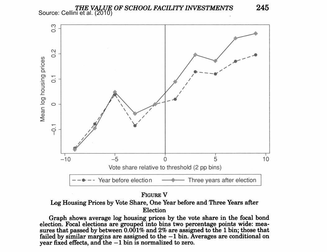
Figure V

Log Housing Prices by Vote Share, One Year before and Three Years after Election

Graph shows average log housing prices by the vote share in the focal bond election. Focal elections are grouped into bins two percentage points wide: mea- sures that passed by between 0.001% and 2% are assigned to the 1 bin; those that failed by similar margins are assigned to the -1 bin. Averages are conditional on year fixed effects, and the -1 bin is normalized to zero.

uniformly significant after year 0. The estimates indicate that the TOT effect of bond approval in year t is to increase average prices by 2.8%-3.0% that year, 3.6%-4.1% in year t + 1, 4.2%-8.6% in years t + 2 through t + 5, and 6.7%-10.1% in t + 6. Figure VI plots the coefficients and confidence intervals from the two dynamic specifications, showing estimates out to year 15. The recursive estimator shows growing effects through almost the entire period, whereas the one-step estimator yields a flatter profile. Confidence intervals are wide, particularly for the recursive estimator in later periods, and a zero effect is typically at or near the lower bound of these intervals.35

As discussed in Section IV, the TOT estimators assume that house prices are unaffected by the likelihood of a future bond

35. We have also estimated models that constrain the TOT to be constant over time. With our one-step estimator, we obtain a point estimate of 4.9% and a standard error of 1.7%.

This content downloaded from 169.229.128.52 on Sun, 17 Mar 2019 18:05:59 UTCAll use subject to https://about.jstor.org/terms

Source: Cellini et al. (2010)

KEY CONSEQUENCE OF TIEBOUT MODEL

It is hard for a local government to redistribute from rich topoor:

If local redistribution is high ⇒

1) Poor flock to the city which provides welfare benefits

2) Rich flee to other cities to avoid paying for redistribution⇒ Local redistribution program will break down

Redistribution programs work better if implemented at higherlevel: state or federal (harder to leave the state or country). Atlocal level, need to have tax-benefit linkage to avoid migration

tax-benefit linkages: The relationship between the taxespeople pay and the government goods and services they getin return.

16

REDISTRIBUTION ACROSS COMMUNITIES

There is currently enormous inequality in both the ability of

local communities to finance public goods and the extent to

which they do so.

Central government can redistribute across communities di-

rectly using taxes and spending but also indirectly by giving

grants to lower levels of government

Higher levels of government can redistribute across lower levels

of government through intergovernmental grants.

We assume in graphical analysis that local community chooses

public spending and private spending according the preferences

of Median voter in the community

17

24 of 35

C H A P T E R 1 0 ■ S T A T E A N D L O C A L G O V E R N M E N T E X P E N D I T U R E S

Public Finance and Public Policy Jonathan Gruber Fourth Edition Copyright © 2012 Worth Publishers

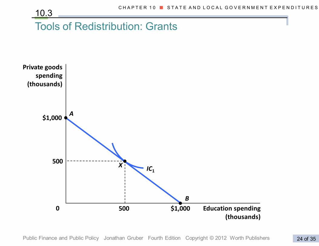
Private goods spending

(thousands)

Education spending (thousands)

0

Tools of Redistribution: Grants

10.3

$1,000

500

500 $1,000

A

B

X IC1

Intergovernmental Grants

Higher level government can provide grants to redistribute

across communities and incentivize communities to spend on

public goods

Three main forms of grants:

1) Matching grant: A grant, the amount of which is tied to

the amount of public good spending by the local community.

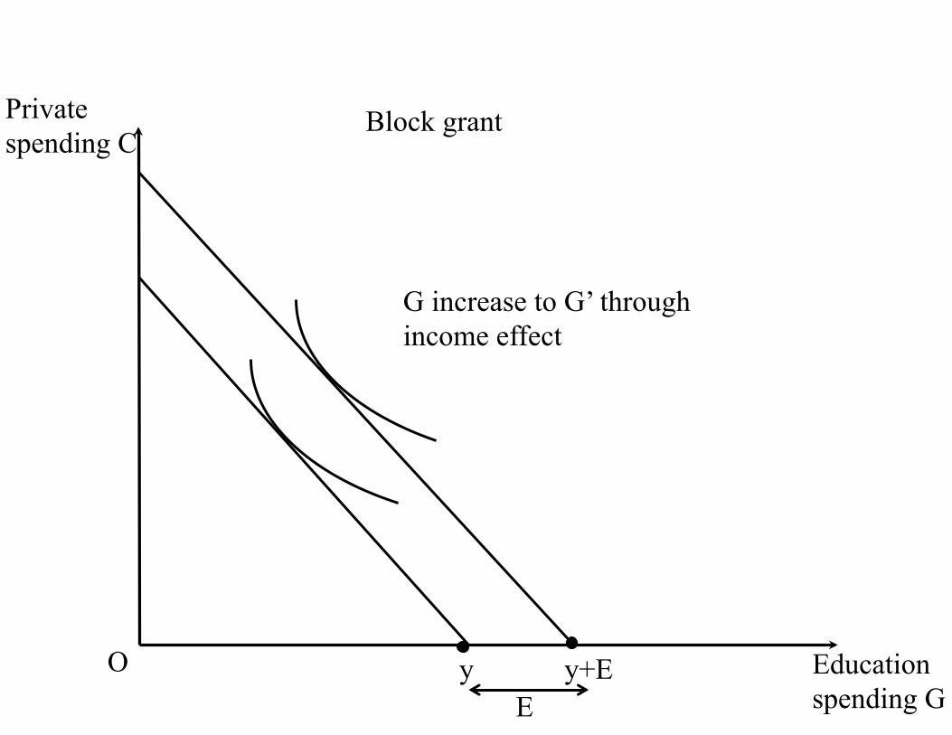
2) Block grant: A grant of some fixed amount with no man-

date on how it is to be spent.

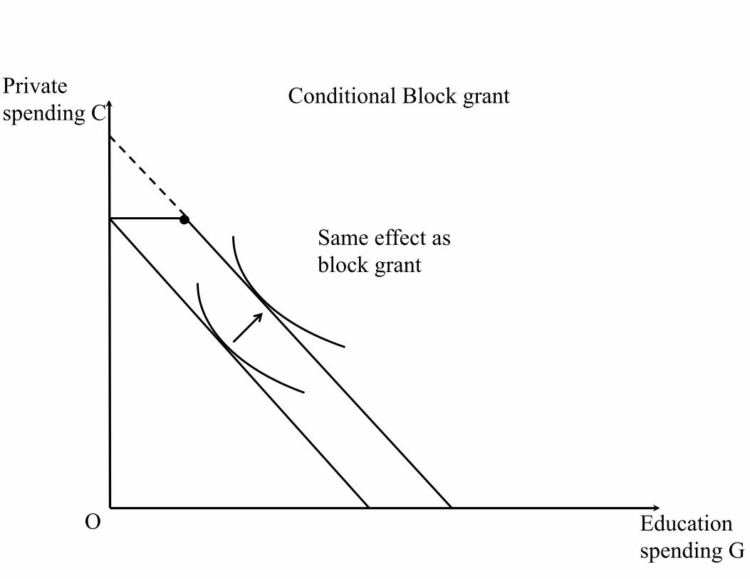
3) Conditional block grant: A grant of some fixed amount

with a mandate that the money be spent in a particular way.

19

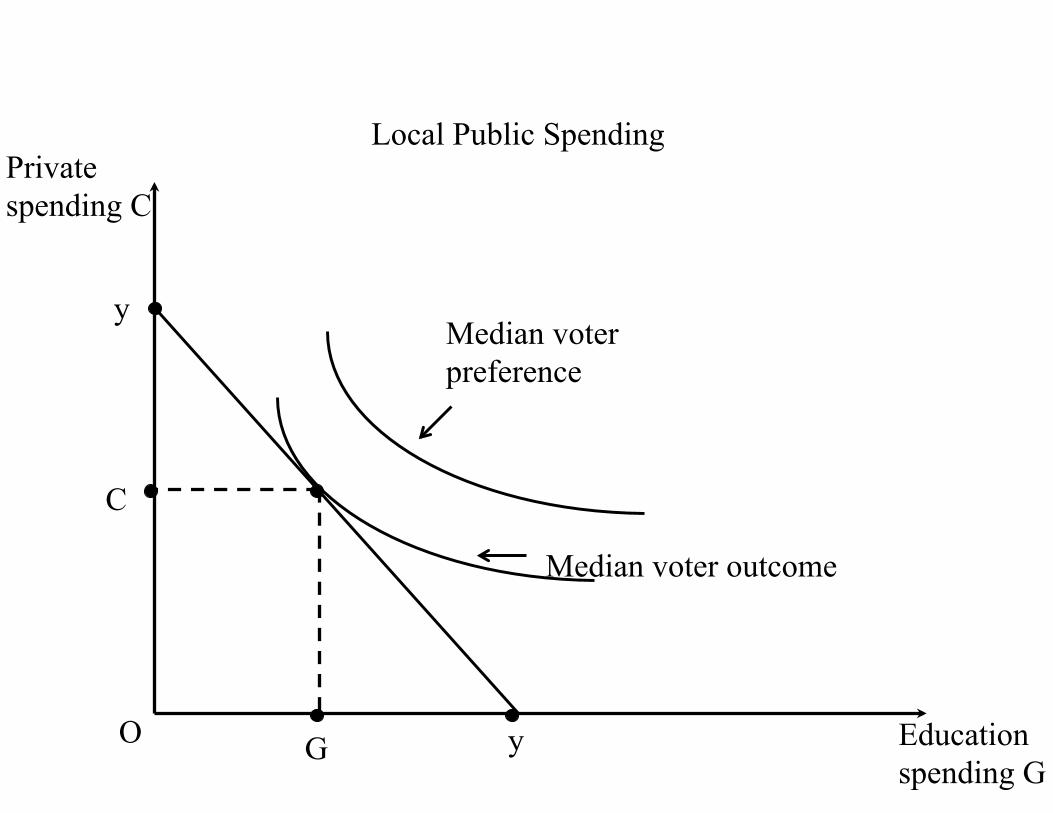
C

Private spending C

Local Public Spending

G

Median voter preference

Median voter outcome

y

y

Education spending G

O

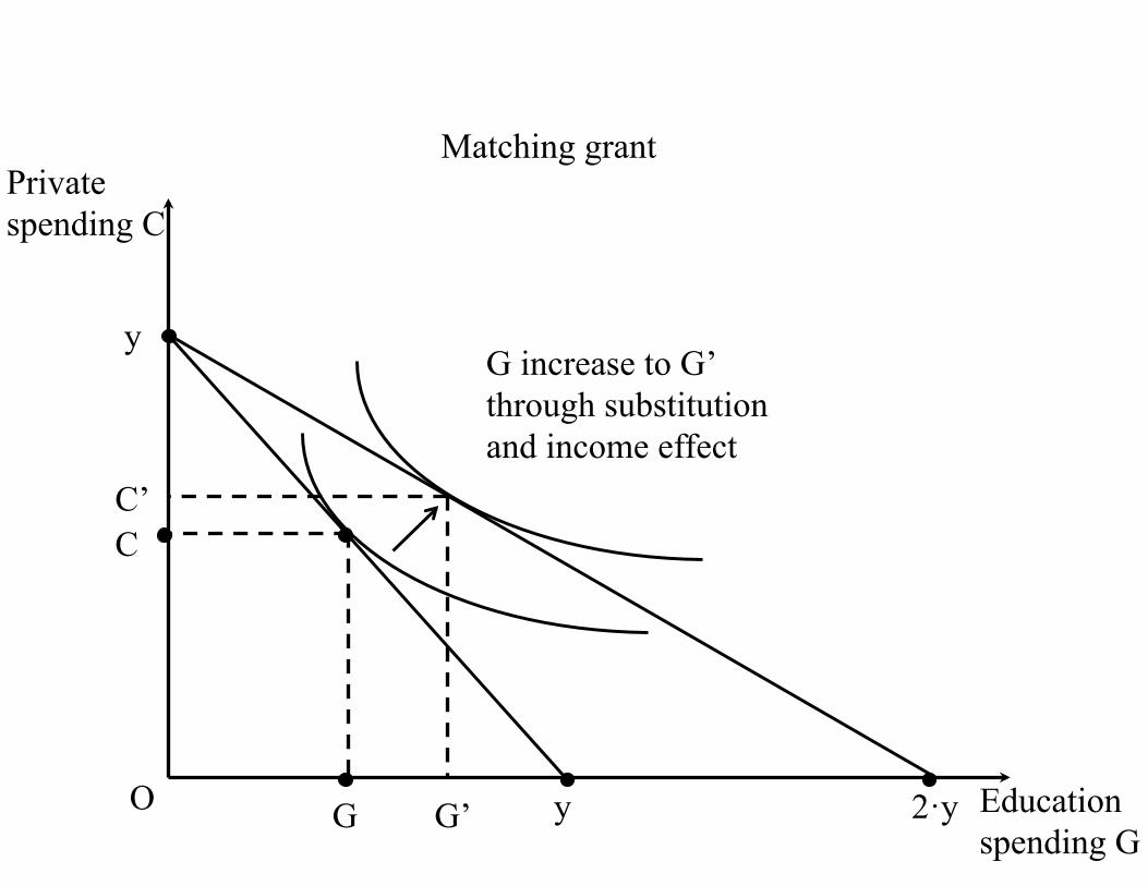
C

Private spending C

Education spending G

G

G increase to G’ through substitution and income effect

y

y

C’

G’ 2·y O

Matching grant

Education spending G

G increase to G’ through income effect

y y+E E

Private spending C

O

Block grant

Private spending C

Education spending G

Conditional Block grant

Same effect as block grant

O

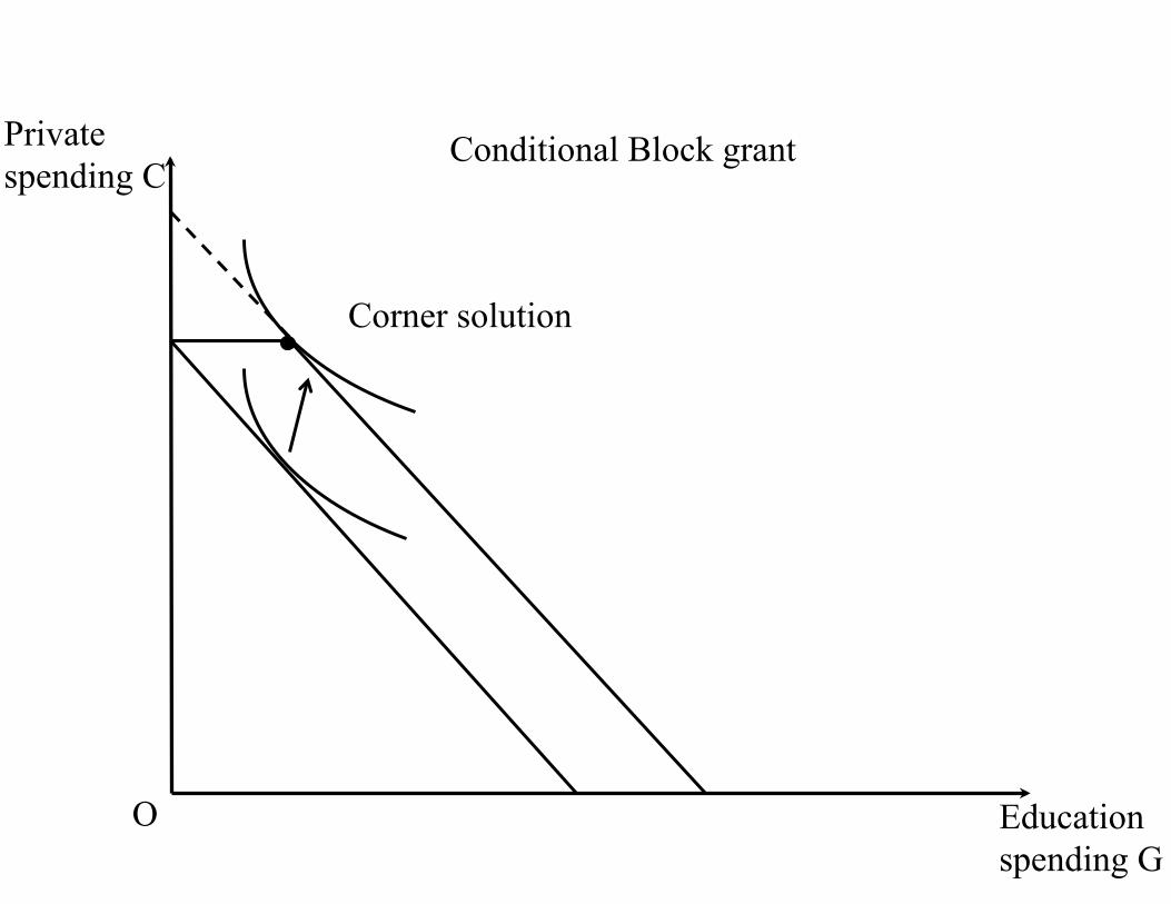
Private spending C

Education spending G

Conditional Block grant

Corner solution

O

KEY PREDICTION OF THEORY: CROWD-OUT

In the theory presented, a $1000 increase in private incomehas the same effect as a $1000 increase in Fed block grant:both shift the budget in the same way and lead to the sameoutcome

Example: $1000 private income increase leads to $800 more inprivate consumption and $200 more in local taxes and publicspending. $1000 extra fed grant leads to $200 extra in publicgood spending and $800 cut in local taxes and hence $800extra in private consumption

Similarly, with multiple public goods (e.g., schools and police),an extra $1000 Fed grant for school has the same effect onschools and police than a $1000 Fed grant for police

Money is fungible: only total resources matter for the alloca-tion across private good and public goods at the local level

21

THE FLYPAPER EFFECT

Hines and Thaler JEP’95 found that the crowd-out of state

spending by federal spending is low and often close to zero

Economist Arthur Okun described this as the flypaper effect

because “the money sticks where it lands” instead of replacing

state spending

But evidence is based on correlation [not necessarily causation

as states that get grants maybe the ones that like spending

the most]

Recent studies show that there is a flypaper effect in the short-

run but that there is substantial crowd-out from block grants

in the long-run

22

REDISTRIBUTION IN ACTION:

SCHOOL FINANCE EQUALIZATION

School finance equalization: Laws that mandate redistribu-

tion of funds across communities in a state to ensure more

equal financing of schools.

Without school finance equalization, huge disparity in property

tax base and hence school funding (per pupil) across areas

(example from Bay Area: Lafayette is very wealthy, Richmond

is poor)

Many states (including California) impose equalization: pool

local taxes at state level and redistribute them across districts

Equalization often imposed by courts without thinking care-

fully about economic consequences

23

REDISTRIBUTION IN ACTION:

SCHOOL FINANCE EQUALIZATION

Implicit tax on local government tax revenue: For school

equalization schemes, for $1 of extra local taxes, how much

the central govt takes away in reduced transfers to local govt

1) With no equalization, the tax rate is 0% (local govt keeps

all its revenue)

2) With perfect equalization, the tax rate is 100% (raising

local revenue has zero impact on local spending)

24

CALIFORNIA SCHOOL EQUALIZATION

In 1960s-1970s, California used to have one of the best K-12public school systems in the nation, now it has one of theworst

California used to have no school finance equalization andhence big disparities across areas

1976: Serrano vs. Priest case: California Supreme court ruledthat disparities above a threshold were unconstitutional

⇒ Wealthy districts forced to give all their tax revenue abovethe threshold to the common pool to fund poor districts

⇒ local government has no incentive to raise taxes ⇒ taxesand school funding fall in rich districts

⇒ Property taxes no longer able to fund schools adequately

25

CALIFORNIA PROPOSITION 13

In 1970s, discontent among the public about growing propertytaxes in CA due to (1) fast housing price increases and (2)local property taxes no longer funded local schools due toschool equalization (prop tax not capitalized into local prices)

Proposition 13 was voted in 1978 and imposed strong limitson property taxes (and required super majority 2/3 vote instate legislature to increase ANY tax):

Assessed value of real estate property can only grow at mostby 2% per year (instead of following price increases which arearound 4-5% on average)

⇒ Property owners no longer face big increases in prop tax (helps retireeson fixed income)

⇒ New owners end up paying much more than old owners (e.g., houseassessed at $200K that sells for $1m will see a 5-fold increase in propertytaxes). Creates a lock-in effect (Ferreira 2010)

26

REFERENCES

Jonathan Gruber, Public Finance and Public Policy, Fifth Edition, 2016Worth Publishers, Chapter 10

Cellini, Stephanie, Fernando Ferreira and Jesse Rothstein. 2010. “TheValue of School Facility Investments: Evidence from a Dynamic RegressionDiscontinuity Design”, Quarterly Journal of Economics, 125(1), 215-261.(web)

Ferreira, Fernando. 2010. “You can take it with you: Proposition 13 taxbenefits, residential mobility, and willingness to pay for housing amenities.”Journal of Public Economics 94(9-10), 661-673. (web)

Hines, James R., and Richard H. Thaler. “Anomalies: The flypaper ef-fect.” The Journal of Economic Perspectives 9.4 (1995): 217-226.(web)

Hoxby, Caroline M. “Does Competition among Public Schools Benefit Stu-dents and Taxpayers?.” The American Economic Review 90.5 (2000):1209-1238.(web)

Oates, Wallace E. 1969. “The Effects of Property Taxes and Local PublicSpending on Property Values: An Empirical Study of Tax Capitalizationand the Tiebout Hypothesis” Journal of Political Economy 77(6), 957-971.(web)

27

Rothstein, Jesse. ”Does Competition Among Public Schools Benefit Stu-dents and Taxpayers? Comment.” The American Economic Review 97.5(2007): 2026-2037.(web)

Tiebout, Charles M. “A pure theory of local expenditures.” The Journalof Political Economy 64.5 (1956): 416-424.(web)