11

Theory of Groundwater FlowTheory of Groundwater Flow

Topics1. Differential Equations of Groundwater

Flow2. Boundary conditions3. Initial Conditions for groundwater

problems4. FlowNet analysis5. Mathematical analysis of some simple

flow problems

22

5.1. Differential Equations5.1. Differential Equations

Examples of useful use of flow equations in solving Hydro Problems

(1) WL drop around a well after 10 years of pumping

(2) Contaminant concentration changes after 5 years of remediation (cleanup)

(3) Change in storage of aquifer after use of 50 years

33

Mathematical approach Mathematical approach

• Represent the GROUNDWATER process

by an equation

• Solving the equation

• Result is hydraulic head (space, time)

44

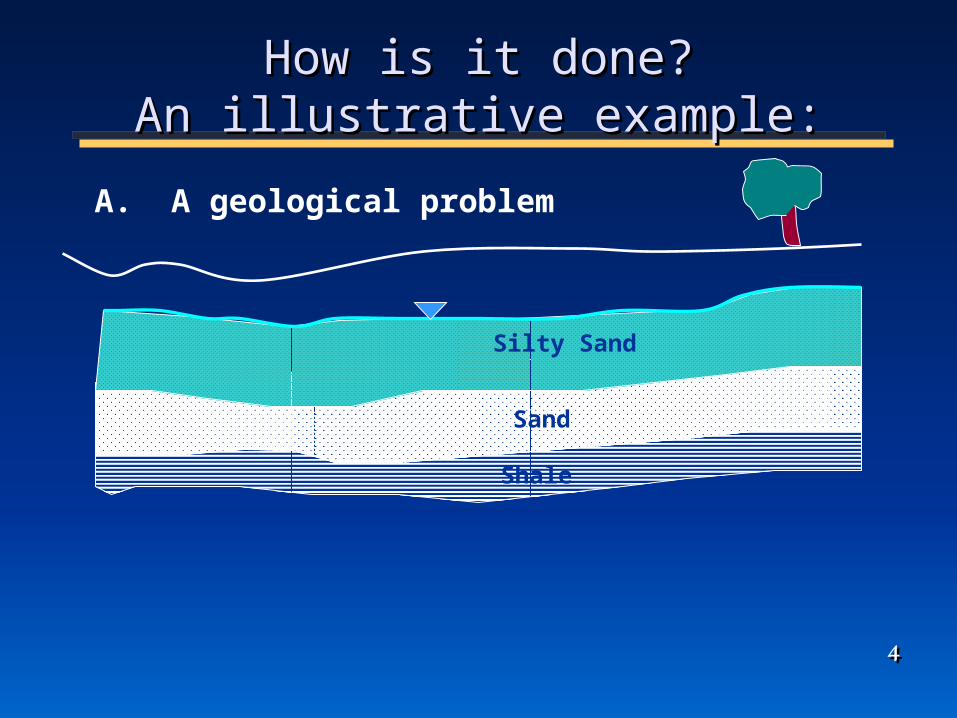
How is it done?How is it done?An illustrative example:An illustrative example:

Silty Sand

Sand

Shale

A. A geological problem

55

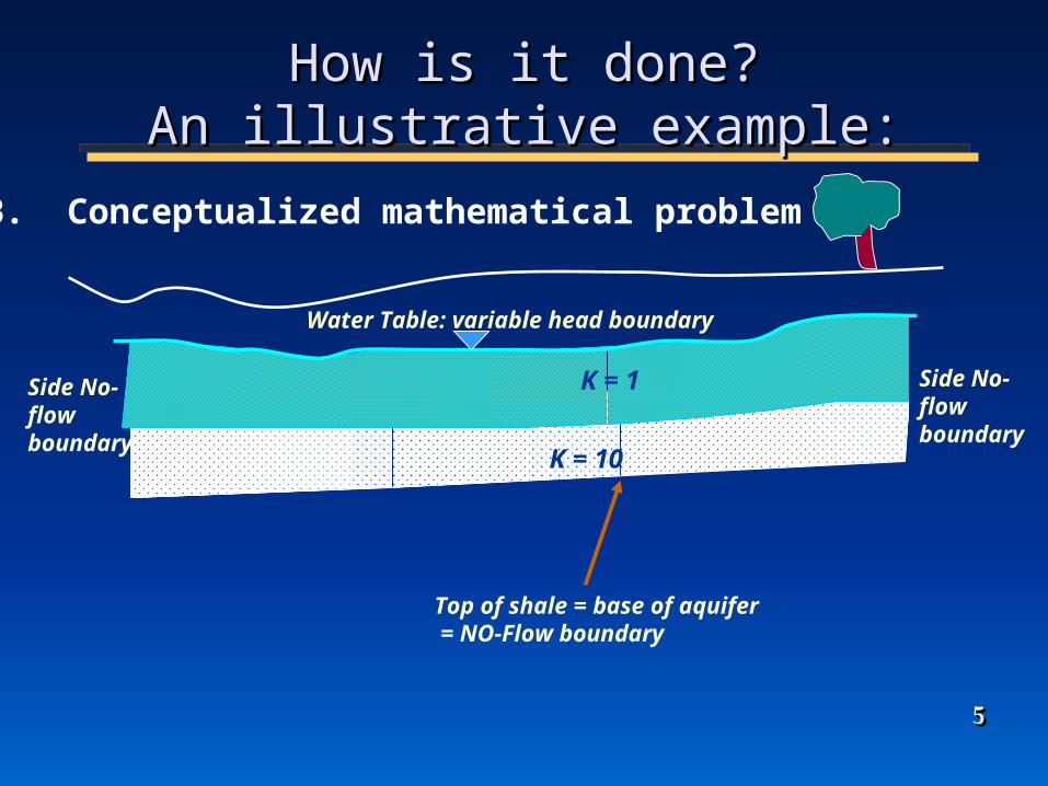
How is it done?How is it done?An illustrative example:An illustrative example:

K = 1

K = 10

B. Conceptualized mathematical problem

Water Table: variable head boundary

Top of shale = base of aquifer = NO-Flow boundary

Side No-flow boundary

Side No-flow boundary

66

How is it done?How is it done?An illustrative example:An illustrative example:

K = 1

K = 10

C. Calculating the hydraulic head distribution(governing equations)

h= 90888684828078

76

K = 1

K = 10

77

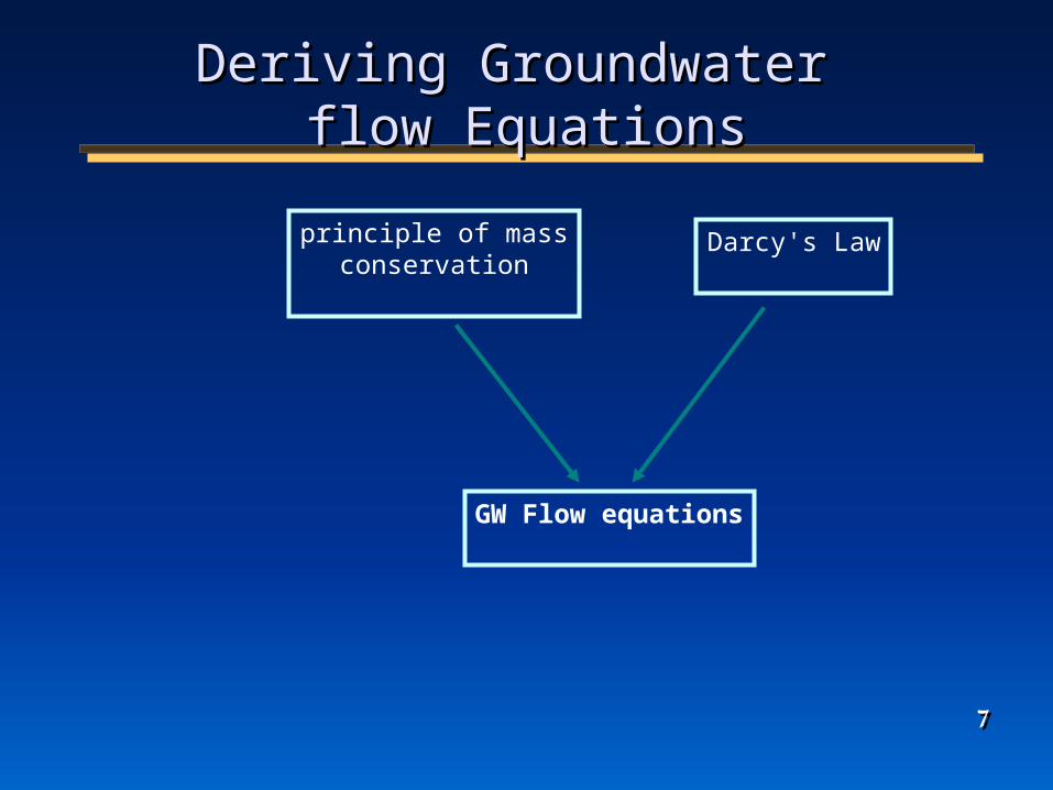
Deriving Groundwater Deriving Groundwater flow Equationsflow Equations

Darcy's Lawprinciple of mass conservation

GW Flow equations

88

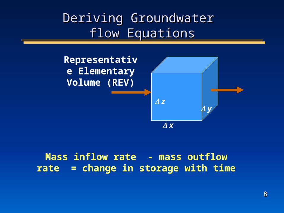
Representative Elementary

Volume (REV)

Mass inflow rate - mass outflow rate = change in storage with time

x

y z

Deriving Groundwater Deriving Groundwater flow Equationsflow Equations

99

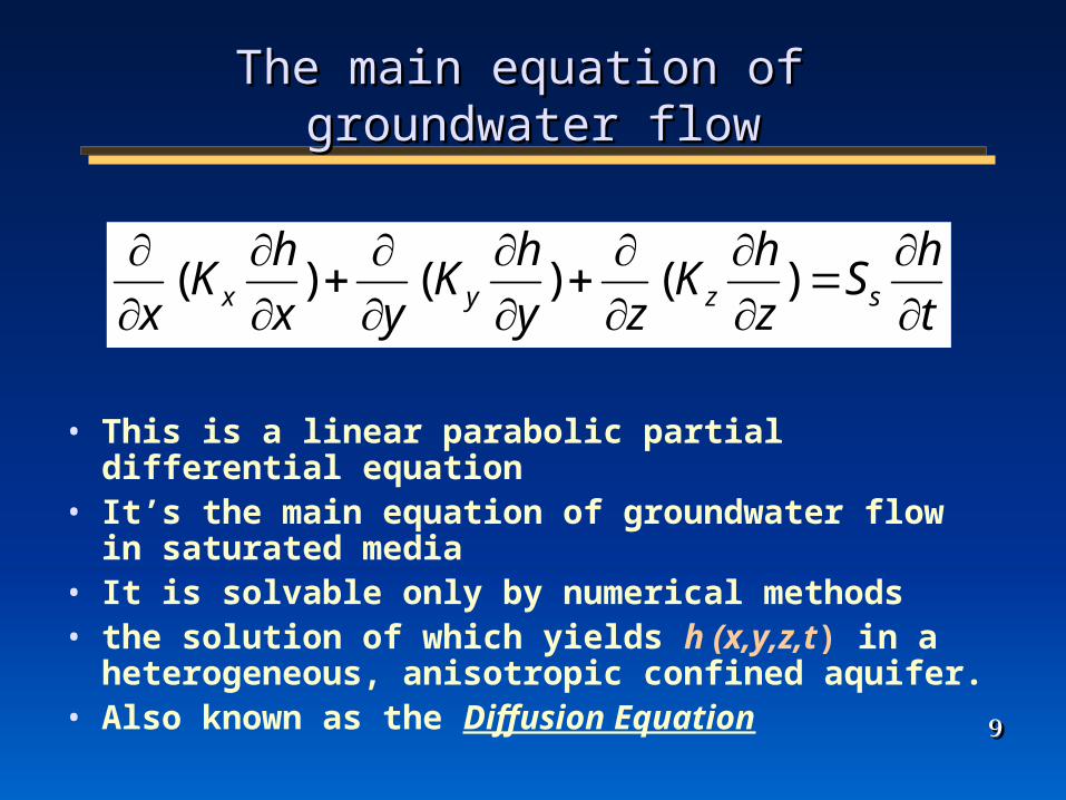
The main equation of The main equation of groundwater flowgroundwater flow

• This is a linear parabolic partial differential equation• It’s the main equation of groundwater flow in

saturated media• It is solvable only by numerical methods• the solution of which yields h (x,y,z,t) in a

heterogeneous, anisotropic confined aquifer.• Also known as the Diffusion Equation

x

Kh

x yK

h

y zK

h

zS

h

tx y z s( ) ( ) ( )

1010

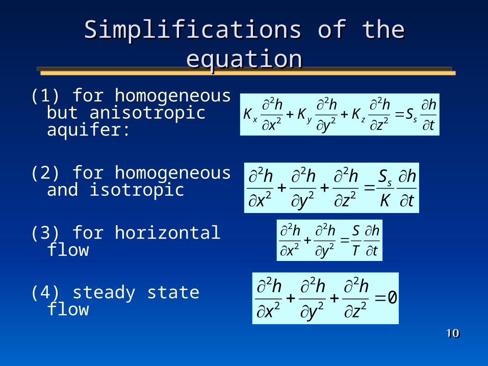
Simplifications of the equationSimplifications of the equation

(1) for homogeneous but anisotropic aquifer:

(2) for homogeneous and isotropic

(3) for horizontal flow

(4) steady state flow

Kh

xK

h

yK

h

zS

h

tx y z s

2

2

2

2

2

2

2

2

2

2

2

2

h

x

h

y

h

z

S

K

h

ts

2

2

2

2

h

x

h

y

S

T

h

t

2

2

2

2

2

20

h

x

h

y

h

z

1111

Laplace equationLaplace equation

• one of the most useful field equations employed in hydrogeology. The solution to this equation describes the value of the hydraulic head at any point in a 3-dimensional flow field

• Note: the mapped potentiometric surface represents "solution" to Laplace's equation for 2-dimensional flow field

2

2

2

2

2

20

h

x

h

y

h

z

1212

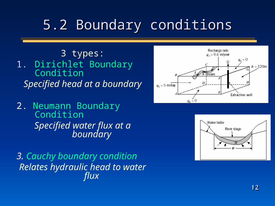
5.2 Boundary conditions5.2 Boundary conditions

3 types:1. Dirichlet Boundary

ConditionSpecified head at a boundary

2. Neumann Boundary ConditionSpecified water flux at a

boundary

3. Cauchy boundary conditionRelates hydraulic head to water

flux

1313

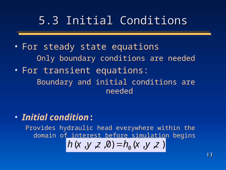
5.3 Initial Conditions5.3 Initial Conditions

• For steady state equationsOnly boundary conditions are needed

• For transient equations:Boundary and initial conditions are needed

• Initial condition:Provides hydraulic head everywhere within the domain of interest

before simulation begins

0( , , ,0) ( , , )h x y z h x y z

1414

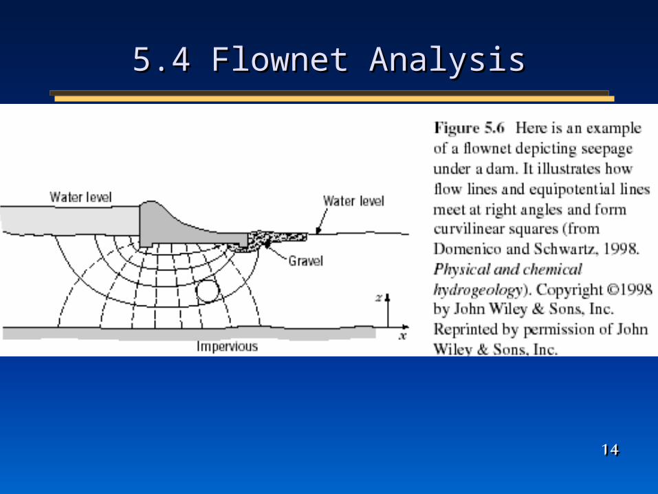
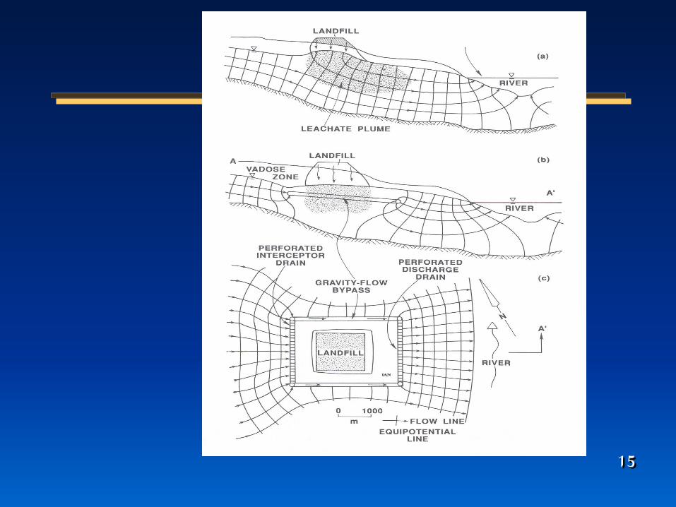
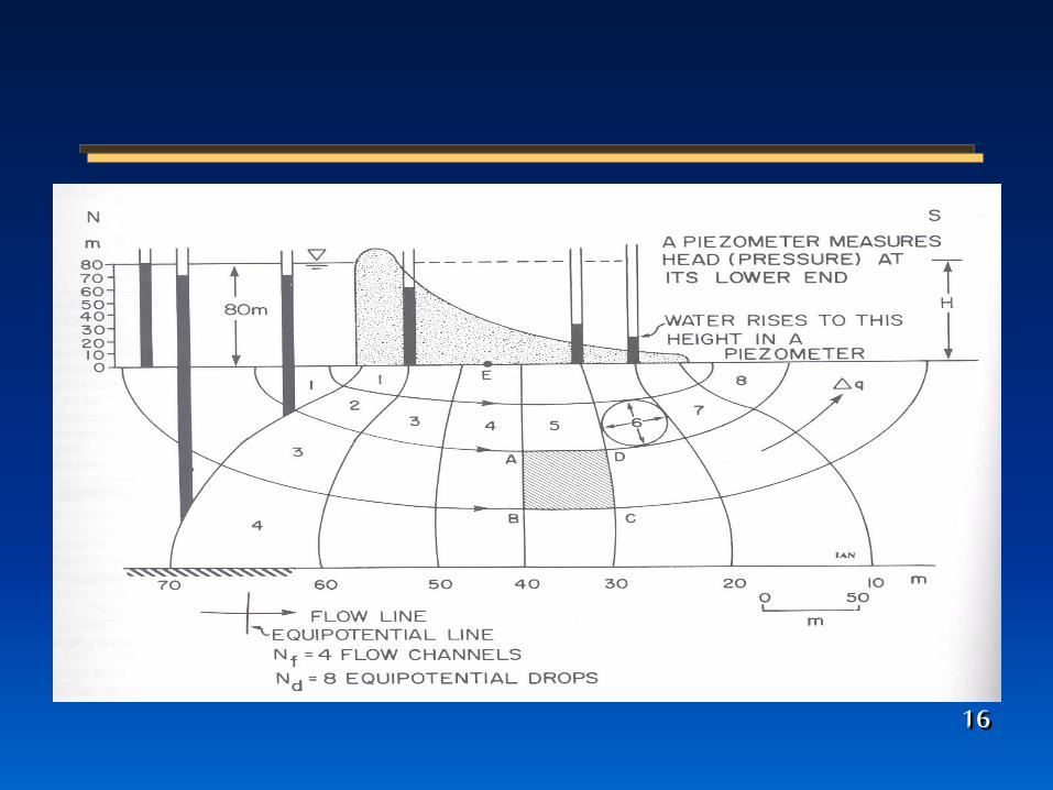
5.4 Flownet Analysis5.4 Flownet Analysis

1515

1616

1717

Flownets, general features in a 2-D flow domain Flownets, general features in a 2-D flow domain

• 1. Streamlines are perpendicular to equipotential lines. If the hydraulic-head drops between the equip. lines are the same, the streamlines and equip. lines form curvilinear squares.

• 2. The same quantity of ground water flows between adjacent pairs of flow lines, provided no flow enters or leaves the region in the internal part of the net. It follows, then that the number of flow channels (known as stream tubes) must remain constant throughout the net.

• 3. The hydraulic-head drop between two adjacent equipotential lines is the same.

1818

Flownets, strategies for constructionFlownets, strategies for construction

1. Study well-constructed flownets and try to duplicate them by independently reanalyzing the problems they represent

2. In a first attempt, use only four or five flow channels.3. Observe the appearance of the entire flownet; do not try to

adjust details until the entire net is approximately correct.4. Be aware that frequently parts of a flownet consist of straight

and parallel lines, result in uniformly sized squares. 5. In a flow system that has symmetry, only a section of the net

needs to be constructed because the other parts are images of that section.

6. During the sketching of the net, keep in mind that the size of the rectangle changes gradually; all transitions are smooth, and where the paths are curved they are of elliptical or parabolic shape.

1919

Flownets, RulesFlownets, Rules

1. A no-flow boundary is a streamline2. The water table is a streamline when there is no flow

across the water table, that is, no recharge or ET. When there is recharge, the water table is neither a flow line nor an equipotential line.

3. Streamlines end at extraction wells, drains, and gaining streams, and they start from injection wells and losing streams.

4. Lines dividing a flow system into two symmetric parts are streamlines.

5. In natural ground-water systems, streamlines often begin and end at the water table in areas of ground-water recharge and discharge, respectively.

2020

• From Darcy’s Eqn in one flow channel in 2-D:

• If we have squares:

5.4 Flownet Analysis5.4 Flownet Analysis

hQ T W

L

f

d

nQ T H

n

2121

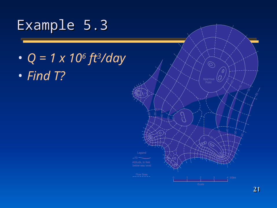
Example 5.3Example 5.3

• Q = 1 x 106 ft3/day

• Find T?

2222

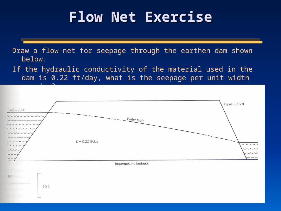
Flow Net ExerciseFlow Net Exercise

Draw a flow net for seepage through the earthen dam shown below.

If the hydraulic conductivity of the material used in the dam is 0.22 ft/day, what is the seepage per unit width per day?

2323

2424

2525

Flownets in Heterogeneous MediaFlownets in Heterogeneous Media

hQ T W

L

2

222

1

111 L

WhT

L

WhTQ

12

21

2

1

WL

WL

T

T

For same hydraulic drop, h1 = h2

2626

Example 5.4

2727

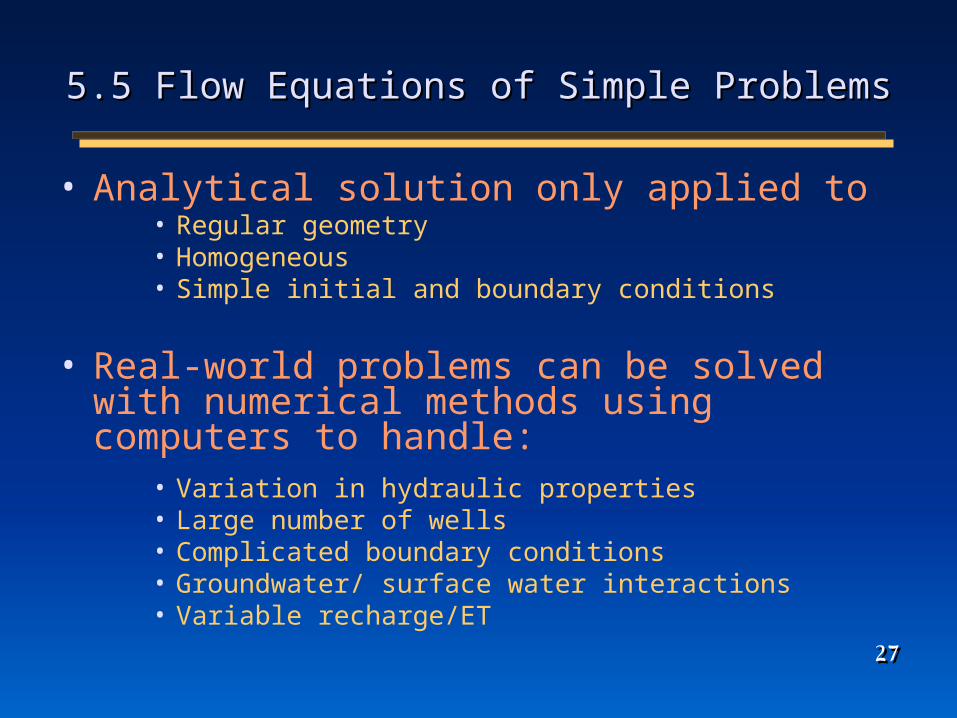
5.5 Flow Equations of Simple Problems5.5 Flow Equations of Simple Problems

• Analytical solution only applied to• Regular geometry• Homogeneous • Simple initial and boundary conditions

• Real-world problems can be solved with numerical methods using computers to handle:

• Variation in hydraulic properties• Large number of wells• Complicated boundary conditions• Groundwater/ surface water interactions• Variable recharge/ET

2828

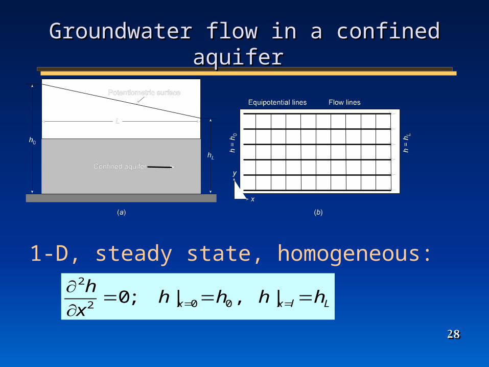
Groundwater flow in a confined aquifer Groundwater flow in a confined aquifer

1-D, steady state, homogeneous:

Llxx hhhhx

h

| ,| ;0 002

2

2929

Example 5.5

3030

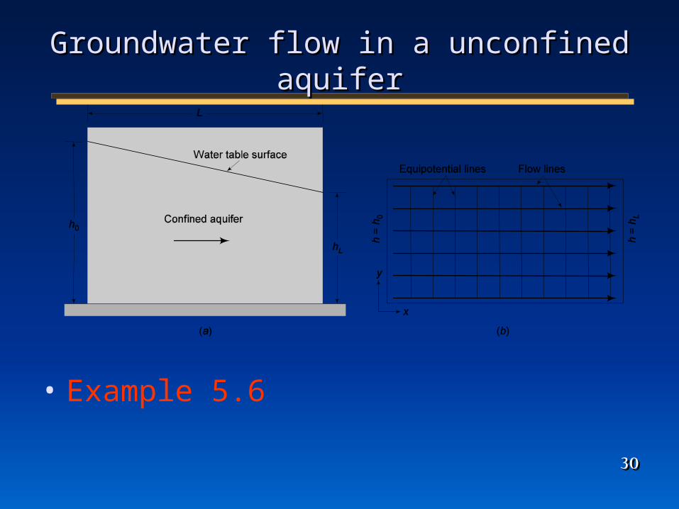
Groundwater flow in a unconfined aquiferGroundwater flow in a unconfined aquifer

• Example 5.6

3131

Chapter HighlightsChapter Highlights

1. Ground-water hydrologists rely on quantitative mathematical approaches in analyzing test data and in making predictions about how systems are likely to behave in the future. The mathematical approach involves representing the flow process by an equation and solving it. The solution within some domain or region of interest defines how the hydraulic head varies as a function of space and time.

2. The flow equations are complicated partial differential equations. Fortunately, at this introductory level, all one really needs to do is to identify the equation and extract a few details. In most applications, the solutions are available in simplified forms. To find the unknown in an equation, simply find the variable residing in the derivative term.

3. Equations of ground-water flow can be developed, starting with an appropriate conservation statement of this form

mass inflow rate, -mass outflow rate = change of mass storage with time The general approach is to apply this equation to a block of porous medium called a

representative elementary volume. It is possible to replace the words in this equation by mathematical expressions, transforming it to a form that can be developed to the main equation of ground-water flow in a porous medium

3232

Chapter HighlightsChapter Highlights

4. The solution of differential equations requires boundary conditions. In effect, the boundary conditions stand in for the conditions outside of the simulation domain and effectively let one concentrate the modeling on the simulation domain.

5. There are three types of common boundary conditions. The first type or Dirichlet condition involves providing known values of hydraulic head along the boundary. The second type or Neumann condition requires specification of water fluxes along a boundary. A no-flow boundary (water flux zero) is the most well-known second-type boundary condition. The third-type or Cauchy boundary condition relates hydraulic head to water flux. This boundary condition is commonly used to represent ground-water/surface-water interactions.

6. For transient equations, in which the hydraulic head can change as a function of time, it is necessary to define the initial condition. The initial condition provides the hydraulic head everywhere within the domain of interest before the simulation begins (that is, at time zero).

3333

Chapter HighlightsChapter Highlights

7. A variety of mathematical and graphical approaches are available to solve ground-water- flow equations. One approach that is emphasized in this chapter is called the flownet analysis. For relatively simple, two-dimensional, steady-state flow problems, you can determine the distribution of equipotential lines graphically. Starting with an outline of the simulation domain, one adds streamlines and equipotential lines following a set of rules. For example, streamlines and equipotential lines must intersect at right angles to form a set of curvilinear squares. If you are careful, you can develop the unique pattern (and reproducible pattern) that describes flow in the domain.

8. This chapter demonstrates how simple analytical solutions can be used to describe some simple steady-state problems of flow. We will return to analytical solutions again in Chapters 8-11 on well hydraulics and regional ground-water flow.