PseudosplinesAuthor(s): Trevor HastieReviewed work(s):Source: Journal of the Royal Statistical Society. Series B (Methodological), Vol. 58, No. 2(1996), pp. 379-396Published by: Blackwell Publishing for the Royal Statistical SocietyStable URL: http://www.jstor.org/stable/2345983 .Accessed: 18/07/2012 18:28

Your use of the JSTOR archive indicates your acceptance of the Terms & Conditions of Use, available at .http://www.jstor.org/page/info/about/policies/terms.jsp

.JSTOR is a not-for-profit service that helps scholars, researchers, and students discover, use, and build upon a wide range ofcontent in a trusted digital archive. We use information technology and tools to increase productivity and facilitate new formsof scholarship. For more information about JSTOR, please contact support@jstor.org.

.

Blackwell Publishing and Royal Statistical Society are collaborating with JSTOR to digitize, preserve andextend access to Journal of the Royal Statistical Society. Series B (Methodological).

http://www.jstor.org

J. R. Statist. Soc. B (1996) 58, No. 2, pp. 379-396

Pseudosplines

By TREVOR HASTIEt

Stanford University, USA

[Received February 1994. Revised March 1995]

SUMMARY We describe a method for constructing a family of low rank, penalized scatterplot smooth- ers. These pseudosplines have shrinking behaviour that is similar to that of smoothing splines. They require two ingredients: a basis and a penalty sequence. The smoother is then computed by a generalized ridge regression. The family can be used to approximate existing high rank smoothers in terms of their dominant eigenvectors. Our motivating example uses linear combinations of orthogonal polynomials to approximate smoothing splines, where the linear combination and the penalty sequence depend on the particular instance of the smoother being approximated. As a leading application, we demonstrate the use of these pseudosplines in additive model computations. Additive models are typically fitted by an iterative smoothing algorithm, and any features other than the fit itself are difficult to compute. These include standard error curves, degrees of freedom, generalized cross- validation and influence diagnostics. By using a low rank pseudospline approximation for each of the smoothers involved, the entire additive fit can be approximated by a corres- ponding low rank approximation. This can be computed exactly and efficiently, and opens the door to a variety of computations that were not feasible before.

Keywords: CUBIC SMOOTHING SPLINES; EIGENDECOMPOSITION; PENALIZED LEAST SQUARES; RIDGE REGRESSION

1. INTRODUCTION

Let x and y denote a set of n observations. A scatterplot smoother of y against x is a function of the data: s(xo) = S(xo Ix, y), which at each xo summarizes the dependence of y on x, usually in a flexible but smooth way. A smoother is linear if

n

S(xO Ix, y) = s(i, xO, x)yi i=l

for some weights s(i, xo, x) which do not depend on y. Popular linear smoothers are smoothing splines, kernel smoothers and local regression. If we concentrate on the computation of the fit only at the points in x, we can write a linear smoother as a linear map S: Rni-JRn defined by y = Sy. S is commonly referred to as a smoother matrix (Buja et al., 1989; Hastie and Tibshirani, 1990).

S is the smoothing analogue of the hat or projection matrix in regression. Although S typically has full rank (n), we shall see that most of its action is concentrated in a much lower dimensional subspace. Consequently we can approximate S by a lower

tAddress for correspondence: Department of Statistics, Sequoia Hall, Stanford University, Stanford, CA 94305, USA. E-mail: trevor@playfair.stanford.edu

? 1996 Royal Statistical Society 0035-9246/96/58379

380 HASTIE [No. 2,

dimensional operator. Although the techniques that we discuss are quite general, they are motivated by and focus on smoothing splines.

In this paper we describe a method for constructing a family of low rank, penalized scatterplot smoothers. These pseudosplines have shrinking behaviour that is similar to that of smoothing splines. They require two ingredients: a basis and a penalty sequence; the smoother is then computed by a generalized ridge regression. The family can be used to approximate existing high rank smoothers in terms of their dominant eigenvectors. Our leading example uses linear combinations of orthogonal polynomials to approximate smoothing splines, where the linear combination and the penalty sequence depend on the particular instance of the smoother being approximated, but to a negligible extent on the value of the smoothing parameter.

There are several reasons why such a representation is appealing.

(a) The family is simple and low dimensional, like polynomial regression. How- ever, instead of selecting the degree in integral steps, the ridge parameter allows us access to a continuum of models. Besides being a compelling application of ridge regression, this simple model offers much insight into penalized smoothers (see Fig. 2 later).

(b) The family provides a good low rank approximation to an existing smoother S. Although the matrix S is not explicitly required to compute the fit, it is needed for secondary characteristics of the smoother, such as standard errors, degrees of freedom and diagnostics.

(c) Smoothers are often used in a compound way, such as in generalized additive models (Hastie and Tibshirani, 1990), projection pursuit regression (Friedman and Stuetzle, 1981; Roosen and Hastie, 1994) and recently in non-linear auto- regression models (Chen and Tsay, 1993) and other time series applications (Green and Silverman, 1994). Simple approximations allow the fit to be computed directly without iteration. This is especially important in cases where iterative algorithms are inefficient or may fail; autoregressive and time series models with highly correlated predictors fall into this class. Again they also make available secondary characteristics which are even less accessible for these more complicated models.

2. SMOOTHING SPLINES In this section we give a brief review of smoothing splines, which motivate our

pseudosplines. A cubic smoothing spline minimizes the penalized least squares criterion

n +oo

Syi - g(Xi)}2 + A g"(Z)2 dz (1) 1 ~~~~~-00

over a suitable Sobolev space W2 of functions (Silverman, 1985; Wahba, 1990). The solution g(x) is a natural cubic spline with knots at each distinct xi, and for the moment we assume that all the xi in the sample are unique (in Section 7 we show how to deal with ties). The smoothing parameter A trades off smoothness of the curve with its closeness to the y-values. As A -* 0, the solution approaches an interpolating spline, whereas, as A -* oo, the solution approaches the least squares line.

1996] PSEUDOSPLINES 381

One can show that the cubic smoothing spline is a linear smoother and hence write down the smoother matrix for producing the fit at the sample points. Although the standard representation is in terms of the computationally attractive B-spline basis functions, for our purposes that given in Green and Yandell (1985) is more useful:

S =(I+AK-1.

This representation has the n fitted values as parameters. The criterion (1) reduces to Ily- fl + AfTKf, and the quadratic form in the penalty matrix K can be seen roughly to accumulate squared second differences.

Further insight is gained from the eigendecomposition of S or equivalently of K itself. Since S is symmetric, it has a decomposition

n

S= UDUT E iuiuTi (2) i=l

where the columns ui of U are orthonormal and Do is diagonal with elements qi E (0, 1] and decreasing in i. This Demmler and Reinsch (1975) basis has intuitive appeal. The eigenvalue qi shows us how much damping is done to the function ui when the smoother is applied, since Sui = qiui (this also shows that the ui themselves are natural splines). The columns of U are like the sequence of orthonormal polynomials defined on x, in that the number of zero crossings appears to increase with the order. Demmler and Reinsch indeed showed that for k > 3 the number of sign changes in the kth eigenvector of a cubic smoothing spline is k - 1. This decomposition suggests analogies with the traditional smoothing methods for time series (see Rice and Rosenblatt (1983)). UTy expresses y in terms of the basis defined by the columns of U (similar to a Fourier transform). The qi play the role of a taper.

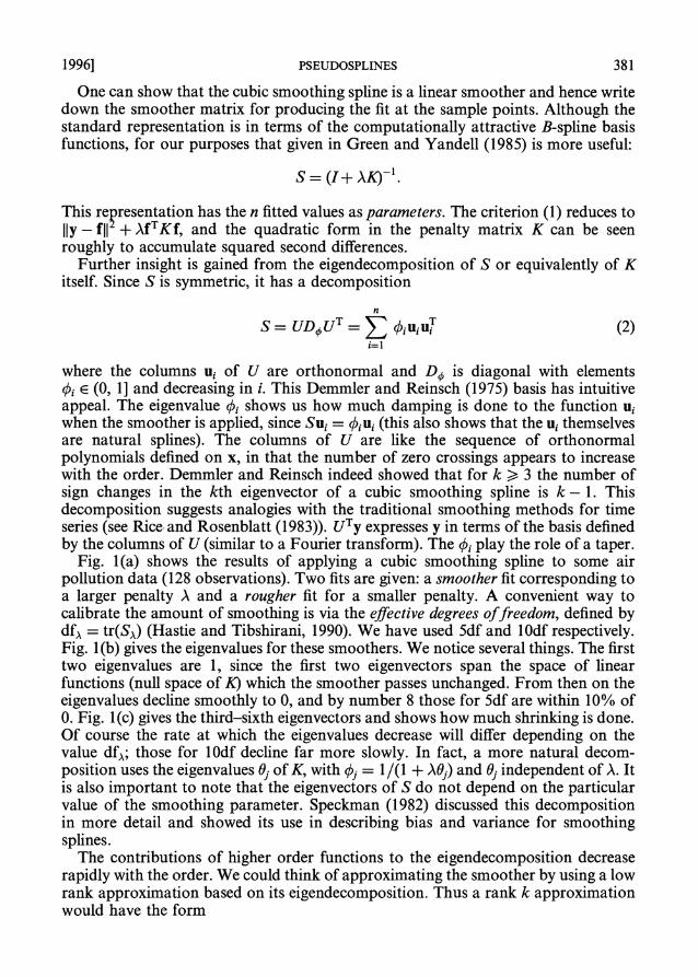
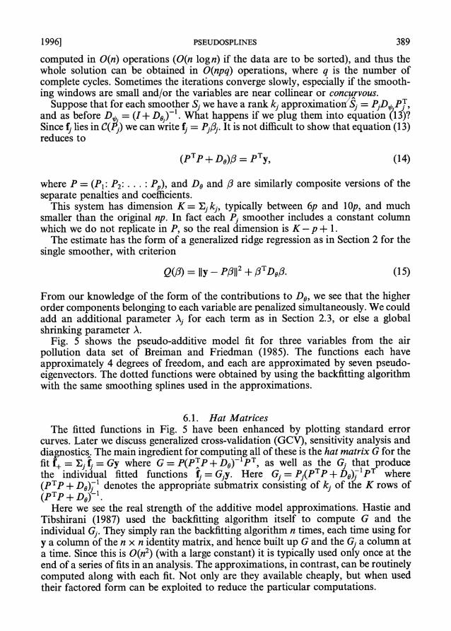
Fig. 1(a) shows the results of applying a cubic smoothing spline to some air pollution data (128 observations). Two fits are given: a smoother fit corresponding to a larger penalty A and a rougher fit for a smaller penalty. A convenient way to calibrate the amount of smoothing is via the effective degrees offreedom, defined by dfA = tr(SA) (Hastie and Tibshirani, 1990). We have used 5df and lOdf respectively. Fig. 1 (b) gives the eigenvalues for these smoothers. We notice several things. The first two eigenvalues are 1, since the first two eigenvectors span the space of linear functions (null space of K) which the smoother passes unchanged. From then on the eigenvalues decline smoothly to 0, and by number 8 those for 5df are within 10% of 0. Fig. 1 (c) gives the third-sixth eigenvectors and shows how much shrinking is done. Of course the rate at which the eigenvalues decrease will differ depending on the value dfA; those for lOdf decline far more slowly. In fact, a more natural decom- position uses the eigenvalues Oj of K, with Oj = 1 /(1 + AOj) and Oj independent of A. It is also important to note that the eigenvectors of S do not depend on the particular value of the smoothing parameter. Speckman (1982) discussed this decomposition in more detail and showed its use in describing bias and variance for smoothing splines.

The contributions of higher order functions to the eigendecomposition decrease rapidly with the order. We could think of approximating the smoother by using a low rank approximation based on its eigendecomposition. Thus a rank k approximation would have the form

382 HASTIE [No. 2,

0~~~~~~*

-50 0 50 100

Daggot Pressure Gradient (a)

0 C;

>

0,

.50 0 50 100 .50 0 so1 s 1 0 1 5 20 25

(b) (C

Fig. l. (a) Smoothing spline fit of ozone concentration versus Daggot pressure gradient (the two fits correspond to different value of the smoothing parameter, chosen to achieve 5 and 10 efective degrees of freedom, defined by df, = tr(S,\)); (b) first 25 eigenvalues for the tWo smoothing spline matrices (the first two are exactly l, and all are greater than or equal to 0); (c) third-sixth eigenvectors of the spline smoother matrices (in each case, uj is plotted against x and as such is. viewed as a function of x; the dots on the functions indicate the occurrence of data points; the damped functions represent the smoothed versions of these functions (using the Sdf smoother))

Sk=UDk uT (3)

0~~~~~~S

where Dk is a truncated version of Do with diagonal elements from k + I onwards set to 0. In fact, Sk is the best rank k approximation to S (Frobenius normn).

3. PSEUDOSPLINES

The smoothing spline suggests a way to parameterize a general class of smoothers. All we need are a sequence of orthonormal basis functions and a penalty sequence. For the analogy to be complete, the basis functions should be ordered in complexity. Let p(x) be a k-vector of such functions and Oj j = 1, . . ., k, the penalties. Then the coffesponding pseudosplinle with parameter A minimizes

1996] PSEUDOSPLINES 383

QA(/ y) = IIY- P_pll2 + A/3TD0/3 (4)

where P is the matrix of evaluations of p at the data and Do = diag(9l, . . . Sk). The solution has smoother matrix SA(P, 0) = p(pTp + AD0)-1PT. If in addition the bases are orthonormal with respect to the observed x (sample measure), then pTp = I and our smoother simplifies to SA(P, 0) = P(I+ ADO)- PT. This has the form of the truncated smoothing spline (3) with (I+ AD)-' corresponding to the non-zero block of D4 and P to the corresponding columns of U.

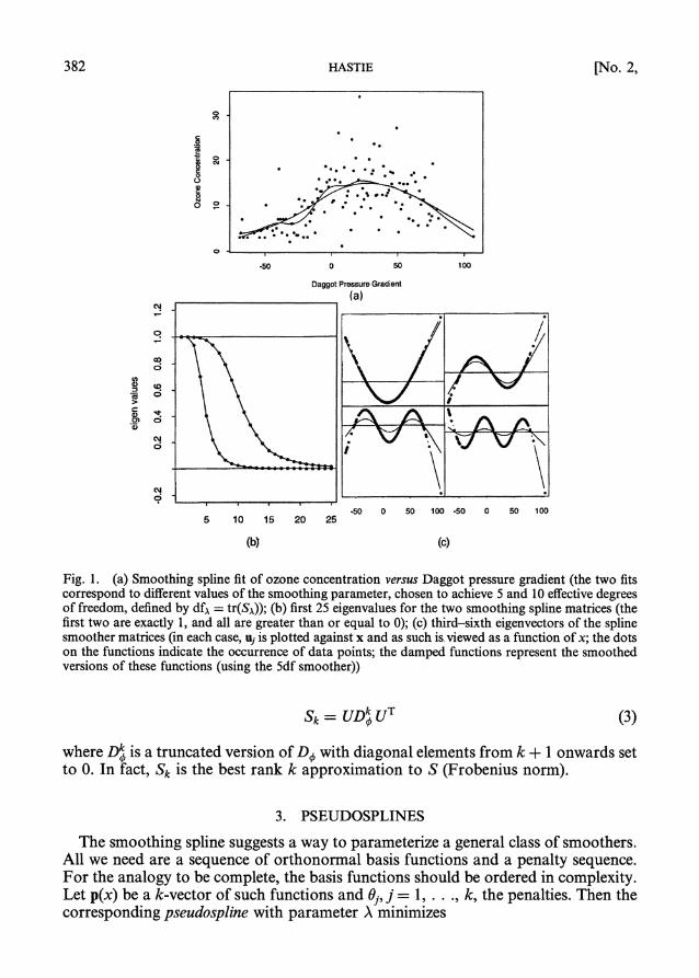
Fig. 2 illustrates the action of a pseudospline in terms of its eigenvalues. How do we choose the bases and penalty sequences? Some obvious choices are

orthogonal polynomials, cosinusoids (Rice and Rosenblatt, 1983) or Legendre or Chebyshev polynomials, where orthogonality is defined in terms of a continuous measure. Rice (1982) studied the rates of convergence of penalized polynomials using the last two systems.

All these candidates are naturally hierarchical they have a complexity ordering (for this reason the popular B-spline bases are not natural candidates). Often it is natural for some of the basis functions to remain unpenalized (their Ojs are 0). For example, we may want the first two basis functions to span the space of linear functions (or possibly a higher order polynomial subspace), and 91 = 02 = 0; this is a direct analogy with the null penalty space of cubic smoothing splines. Some applications may call for specially tailored basis functions and null spaces. Whatever the choice, we end up with a parameterized family that gives us access to a spectrum of models ranging from the fit on the null space at one extreme to the unpenalized fit on the full basis set at the other.

Recently Donoho and Johnstone (1994) have applied non-linear shrinkage schemes to bases of orthonormal wavelets; these are more adaptive schemes than the framework discussed here, but similar in spirit.

N CM~~~~~~~~~~~~~~~~~~~~~~~~~~~~~C

o - -..0..0-_------------------------------ ..... --,

oR 0 0

(? 100 15 2* 0 1 0s 1 S 2

0 ~~~~~~0

.9)(a (b)(c

w di of w

to 0 0

eightbasisfunctionsandshrinkigtheir.effec d ownto.5.effective degrees.of.freedom;)soot

5 10 15 20 5 10 15 20 5 10 15 20

Order Order Order

(a) (b) (c)

Fig. 2. Illustration of three different types of smoother based on a series of orthogonal basis functions (shown are the first 20 eigenvalues, and all smoothers have 5 effective degrees of freedom): (a) traditional series smoother, a projection using the first five basis functions; (b) pseudospline, here using eight basis functions and shrinking their effect down to 5 effective degrees of freedom; (c) smoothing spline-none of the eigenvalues are 0

384 HASTIE [No. 2,

For the remainder of this paper we shall focus on using these pseudosplines to approximate existing smoothers, in particular smoothing splines.

4. PSEUDO-EIGENDECOMPOSITION

To fix ideas suppose that we wish our pseudospline to approximate the action of the smoothing spline used in Fig. 1. Our approach is to estimate its truncated eigendecomposition (3). It does not matter which version (rough or smooth) we use, since the eigenvectors are the same, and the eigenvalues 4j give us 0j up to a constant; hence we simply refer to the smoother as S.

We could simply compute S itself and truncate its eigendecomposition. This is expensive (O(n3)), requires S explicitly and defeats the purpose of the approximation. Instead we supply a surrogate or pseudobasis P, which we use to define a pseudo- eigendecomposition of S:

S(P) = PD,,,P (5)

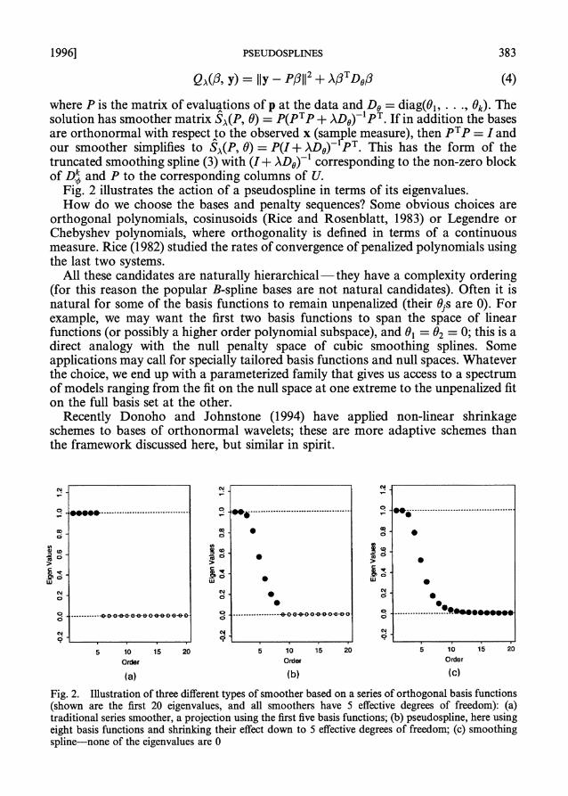
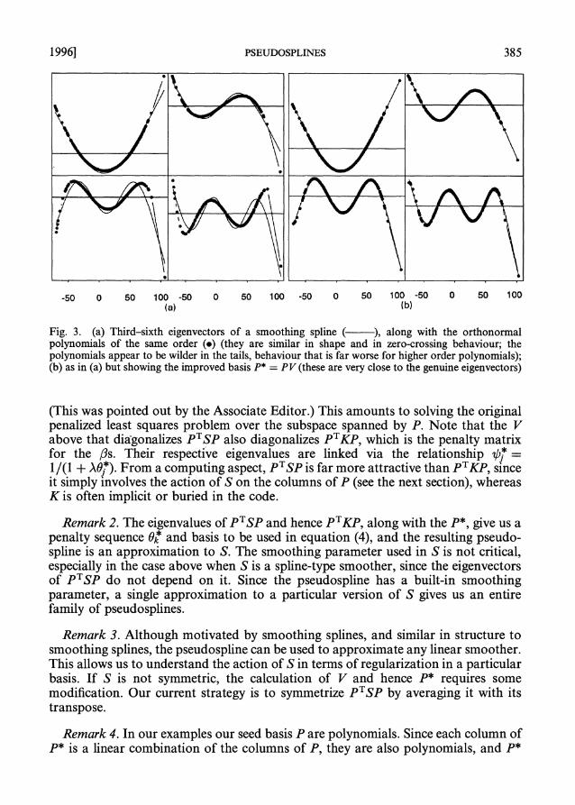
where Dl,, is a k x k diagonal matrix of pseudo-eigenvalues with elements 0i = p7TSp1 = pfT^, and pj is simply the result of smoothing pj (O(n) computations). Proposition f shows that this choice of D, is optimal in a least squares sense. Natural choices for P are the orthonormal polynomials in x. If P is Uk itself, then the V)j are the corresponding eigenvalues of S. Fig. 3(a) shows the third-sixth-order ortho- normal polynomials superimposed on the corresponding eigenvectors of S for our example.

It turns out that we can do better than equation (5) with very little extra work. Consider the k x k eigendecomposition PTSP = VD2* VT, and define P* = PV. Then S(P*) is a better'approximation to S than S(P) is.

Proposition 1. Let P be any n x k orthonormal basis, S a symmetric (smoother) matrix and P* be defined as above. Then

(a) JIS - S(P)IIF = min IS - PDPT IF, D diagonal

(b) IS - S(P*)IIF = min |IS- PMP IF5

(C) II S-S(P*)IIF II l- S(P)IIF-

Proof. Both IS - PMPT IIF and ipTSp - MIIF are minimized by the same matrix M. The results follow immediately by matching elements of M (or D) with the corresponding elements of pTSP. The inequality in (c) is immediate since the approximations minimize the norm subject to conditions of nested generality. El

The pseudo-eigenvalues are indistinguishable from the corresponding genuine components in Fig. 1. On the log-scale, we start to see differences in the very small eigenvalues (10-5). The pseudo-eigenvectors are also very close, especially for low order-see Fig. 3(b).

Remark 1. If S = (I+ AK)-1, then it is not difficult to show that S(P*) solves

mi II Y - PA3112 + A(P)3)TK(P)3). (6) '3

1996] PSEUDOSPLINES 385

-50 0 50 100 -50 0 50 100 -50 0 50 100 -50 0 50 100 (a) (b)

Fig. 3. (a) Third-sixth eigenvectors of a smoothing spline ( ), along with the orthonormal polynomials of the same order (o) (they are similar in shape and in zero-crossing behaviour; the polynomials appear to be wilder in the tails, behaviour that is far worse for higher order polynomials); (b) as in (a) but showing the improved basis P* = PV (these are very close to the genuine eigenvectors)

(This was pointed out by the Associate Editor.) This amounts to solving the original penalized least squares problem over the subspace spanned by P. Note that the V above that diagonalizes PTSP also diagonalizes PTKP, which is the penalty matrix for the ,Qs. Their respective eigenvalues are linked via the relationship i>b= l/(I + A0O). From a computing aspect, pTSp iS far more attractive than pTKP, since it simply involves the action of S on the columns of P (see the next section), whereas K is often implicit or buried in the code.

Remark 2. The eigenvalues of PTSP and hence PTKP, along with the P*, give us a penalty sequence Ok* and basis to be used in equation (4), and the resulting pseudo- spline is an approximation to S. The smoothing parameter used in S is not critical, especially in the case above when S is a spline-type smoother, since the eigenvectors of pT5p do not depend on it. Since the pseudospline has a built-in smoothing parameter, a single approximation to a particular version of S gives us an entire family of pseudosplines.

Remark 3. Although motivated by smoothing splines, and similar in structure to smoothing splines, the pseudospline can be used to approximate any linear smoother. This allows us to understand the action of S in terms of regularization in a particular basis. If S is not symmetric, the calculation of V and hence P* requires some modification. Our current strategy is to symmetrize pTSP by averaging it with its transpose.

Remark 4. In our examples our seed basis P are polynomials. Since each column of P* is a linear combination of the columns of P, they are also polynomials, and P*

386 HASTIE [No. 2,

spans the same space as P since S has full rank. The smoother S(P*) = P(PTSP)PT operates by projecting first onto C(P), smoothing using S, and then reprojecting onto C(P).

Remark 5. Notice that there will be equality in proposition 1 (c) under at least two conditions:

(a) if P = U, a subset of the eigenvectors of S, or (b) if P = P* (so iterating the improvement will not help).

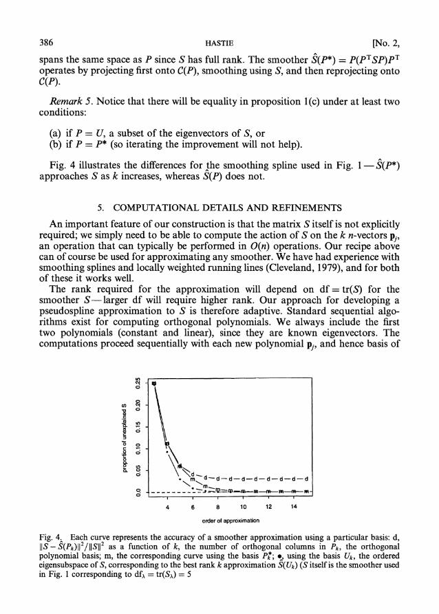
Fig. 4 illustrates the differences for the smoothing spline used in Fig. 1 S(P*) approaches S as k increases, whereas S(P) does not.

5. COMPUTATIONAL DETAILS AND REFINEMENTS

An important feature of our construction is that the matrix S itself is not explicitly required; we simply need to be able to compute the action of S on the k n-vectors pj, an operation that can typically be performed in 0(n) operations. Our recipe above can of course be used for approximating any smoother. We have had experience with smoothing splines and locally weighted running lines (Cleveland, 1979), and for both of these it works well.

The rank required for the approximation will depend on df = tr(S) for the smoother S-larger df will require higher rank. Our approach for developing a pseudospline approximation to S is therefore adaptive. Standard sequential algo- rithms exist for computing orthogonal polynomials. We always include the first two polynomials (constant and linear), since they are known eigenvectors. The computations proceed sequentially with each new polynomial pj, and hence basis of

o.xI o * mX d-d-d-d-d-d-d-d-d a~~~~~

4 6 8 10 12 14

order of approximation

Fig. 4. Each curve represents the accuracy of a smoother approximation using a particular basis: d, IS - S(Pk)J12/JJS112 as a function of k, the number of orthogonal columns in Pk, the orthogonal polynomial basis; m, the corresponding curve using the basis Pk*; .t, using the basis Uk, the ordered eigensubspace of S, corresponding to the best rank k approximation S(Uk) (S itself is the smoother used in Fig. 1 corresponding to dfA = tr(SA) = 5

1996] PSEUDOSPLINES 387

vectors Pj. Although we could compute Pj* sequentially each time, we only need to diagonalize PJTSp1 once the approximation has been found to be satisfactory.

We need to decide how many terms J are sufficient. Ideally, a criterion of the form

F2 IS-S(P )IIF(7) IISIIF

would be informative, but this is unavailable without S. For the present example we used J = 8 polynomials, and F2 was 3.3%. In practice we continue to add terms until

11S(P)- S(PJ-01)1F 211Pj1 SpjI2 + p7 P3 (8)

11 S(PJ*) IIF || P IISJ1F

is below some small threshold (0.001). Once the approximation is satisfactory, we diagonalize PJSPJ to form PJ as described earlier.

To compute the fit f at x when smoothing using S(P*), we use

f = S(P*)y = S p*?/ (P7, Y), (9) j=l

and, to compute the fit f(xo) at a value x0 not among the original xi, we use

A

f(Xo) = 5 p7(xo)''j (p,*, y) (10)

where

pj* (Xo) Pk (XO) Vki k=1

(remember that P* = PJ). We can include a smoothing parameter by replacing i/j by I/(I + AG1), where Oj = I/?pj -1.

Although S(P*) performs better than S(P), they both are based on polynomials and might be dangerous especially when a higher rank approximation is needed. It turns out that we can improve any basis P as an approximation to an eigensubspace of S by smoothing each of the columns using S, followed by an orthogonalization. In the matrix algebra literature this corresponds to an iteration of the Q-R algorithm for finding an eigensubspace of a symmetric matrix. The Q-R algorithm is a generalization of the power method for iteratively finding a single eigenvector. Let QR= SP, where Q is orthogonal and R is the upper triangular matrix that orthog- onalizes SP. ThAen ,(QTSQ)QT is a better approximation to S than is p(pTSp)pT, or, in terms of S, S(Q*) is better than S(P*).

We can be more precise about these improvements.

Proposition 2. Let P be any n x k orthonormal basis and let QR = SP define an improved orthonormal basis Q for approximating the symmetric smoother S with eigenvalues in [0, 1]. Then

388 HASTIE [No. 2,

||S -S(Q*)IIF <- IIS -S(P*)IIF (1

where S(P*) p(pTSp)pT and S(Q*) is defined similarly.

There is strict equality if the columns of P coincide with a subset of the columAns of U, the eigenvectors of S. Notice that the proposition is not stated for S(P) and S(Q); there are counter-examples. A proof of the proposition is given in Appendix A and depends on a lemma proved by Jeff Lagarias. Lagarias (1991) explored inequalities of this nature in a more general context.

Each iteration of this Q-R algorithm requires k - 2 additional applications of the smoother, and an order k eigendecomposition. The need for this added accuracy depends on the particular application. So far we have found that S(P*) is sufficiently accurate for our applications, which typically involve small df.

6. APPLICATION: ADDITIVE MODELS Our motivation for developing pseudosplines was to facilitate some of the difficult

computations required for analysing additive models - this section describes some of these. These are by no means the only applications. Any scenario where smoothing splines and other smoothers are used, especially in a compound, non-standard fashion, can benefit from the parsimonious representation.

The penalized least squares criterion (1) is easily generalized for fitting an additive model

p

Yi = a + E f/(xi) + ei j=l

(Buja et al., 1989):

min E Yi - a-E fj(xj)} + >, jy fj"t(t) 2dt. (12)

fj( )E W2 _ =

It can be shown that the solutions satisfy

I S, S, ... S, fS Sly S2 I S2 *- S2 f2 S2Y

kSP SP SP ... I > fp kspy,

where each of the Sj is the appropriate smoothing spline matrix (each Sj actually represents EjTSjEj where Ej orders x) and fj the vector of evaluations of the ]th function. This np x np system is prohibitively expensive to solve directly-O{(np)3} -although by taking into account the special structure of the smoothing spline matrices can be reduced to an n x n system and hence is 0(n3). Buja et al. (1989) described a backfitting or blockwise Gauss-Seidel algorithm for solving the system iteratively. It is particularly well suited for the job, since the operations Sjz can be

1996] PSEUDOSPLINES 389

computed in O(n) operations (O(n log n) if the data are to be sorted), and thus the whole solution can be obtained in 0(npq) operations, where q is the number of complete cycles. Sometimes the iterations converge slowly, especially if the smooth- ing windows are small and/or the variables are near collinear or conc rvous.

Suppose that for each smoother Sj we have a rank kj approximation = P7DSj and as before D,',. = (I+ DO')'. What happens if we plug them into equation (1 3)? Since fj lies in C(IP) we can write f= Pjp,j. It is not difficult to show that equation (13) reduces to

(pTp + DO)f = pTy (14)

where P = (P1: P2: .. .: Pp), and Do and 13 are similarly composite versions of the separate penalties and coefficients.

This system has dimension K = Ej kj, typically between 6p and lOp, and much smaller than the original np. In fact each Pj smoother includes a constant column which we do not replicate in P, so the real dimension is K - p + 1.

The estimate has the form of a generalized ridge regression as in Section 2 for the single smoother, with criterion

Q(O3) = IIY -_Pp3112 + fTTD9fl. (15)

From our knowledge of the form of the contributions to Do, we see that the higher order components belonging to each variable are penalized simultaneously. We could add an additional parameter Aj for each term as in Section 2.3, or else a global shrinking parameter A.

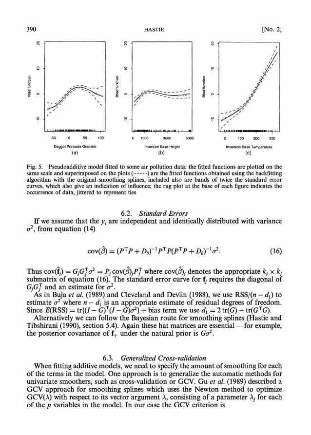
Fig. 5 shows the pseudo-additive model fit for three variables from the air pollution data set of Breiman and Friedman (1985). The functions each have approximately 4 degrees of freedom, and each are approximated by seven pseudo- eigenvectors. The dotted functions were obtained by using the backfitting algorithm with the same smoothing splines used in the approximations.

6.1. Hat Matrices The fitted functions in Fig. 5 have been enhanced by plotting standard error

curves. Later we discuss generalized cross-validation (GCV), sensitivity analysis and diagnostics. The main ingredient for computing all of these is the hat matrix G for the fitf Y 3fj = Gy where G = P(PP+ D)-1pT, as well as the GQ that produce the individual fitted functions f G1y. Here G. = j(pTP + D) 1pT where (pTp + Do)7-. denotes the appropnate submatrix consisting of k. of the K rows of (pTp + D I)1

Here we see the real strength of the additive model approximations. Hastie and Tibshirani (1987) used the backfitting algorithm itself to compute G and the individual Gj. They simply ran the backfitting algorithm n times, each time using for y a column of the n x n identity matrix, and'hence built up G and the Gj a column at a time. Since this is 0(n2) (with a large constant) it is typically used only once at the end of a series of fits in an analysis. The approximations, in contrast, can be routinely computed along with each fit. Not only are they available cheaply, but when used their factored form can be exploited to reduce the particular computations.

390 HASTIE [No. 2,

10 ~ ~ ~ /

a~~~~~~~~~~~~~~~~i Xl I aVI anII X V

-50 O 5s 1 0 10 3000 50X 0 1/0 20 30

Dagot Pressure GradSient Inversion ease Height Inversion Bass Temperature (a) (b) {c)

Fig. 5. Pseudoadditive model fitted to some air pollution data: the fitted functions are plotted on the same scale and superimposed on the plots (- ....... -) are the fitted functions obtained using the backfitting algorithm with the original smoothing splines; included also are bands of twice the standard error curves, which also give an indication of influence; the rug plot at the base of each figure indicates the occurrence of data, jittered to represent ties

6.2. Standard Errors If we assume that the yi are independent and identically distributed with variance

o-11 from equation (I140t)

cov(O (P P + Do)- PTP(PTP + Do)- o2 (16)

Thus co(=GGTa-2 = pj CV jPwhr ov(o)j denotes the appropriate kj x kj

'4 /

submatrix of equation (16). The standard error curve for f reurs the diagonal of GjGT and an estimate for o2 .

As in Buja et al. (1989) and Cleveland and Devlin (1988) we use RSS/(n-dl) to estimate a2where n - d is an appropriate estimate of residual degrees of freedom. Since E(RSS)-=tr{(I -G)T(I -G)o-2 + bias term we use d, = 2 tr(G) -tr(G TG).

Alternatively we can follow the Bayesian route for smoothing splines (Hastie and Tibshirani (I1990), section 5.4). Again these hat matrices are essential -for example, the posterior covariance of f+ under the natural prior is Go'.

6.3. Generalized Cross-validati'on When fitting additive models, we need to specify the amount of smoothing for each

of the terms in the model. One approach is to generalize the automatic methods for univariate smoothers, such as cross-validation or GCV. Gu et al. (1989) described a GCV approach for smoothing splines which uses the Newton method to optimize GCV(A) with respect to its vector argument A consisting of a parameter Aj for each of the p vagtables in the model. In our case the GCV ceBteraon is

1996] PSEUDOSPLINES 391

GCV(A) = n1lI- G(A)y12 (17) tr{I- G(A)}2

where G(A) P(PITP + DAO)-PT and DAB is block diagonal having AjD0. as the ith block. Gu et al. (1989) have a similar form for GCV and discuss several decom- positions for optimizing it efficiently. We shall not go into further details here but point out that all their algorithms are o(K3), where K is the rank of P. In their case, K= n and represents a significant computational cost; here we can use their same algorithms and trade off this computational cost with that incurred by using a rank K approximation to the system.

6.4. Concurvity We can use approximation (14) to gain insight into the nature and stability of the

solutions, exactly here and approximately for the system (13). Buja et al. (1989) introduced the concept of concurvity, which we illustrate here for the case p = 2. Equation (14) reduces to

{ (P2 P I) (O D2) } (2 ) (: PTY;) (18)

Suppose that a column of P1, say u, has correlation 1 with a column of P2, say v. This means that two columns of the left matrix pT P are identical. However, if there are corresponding non-zero entries in the penalty part Do = diag(DO,, Do2), this will not result in a degeneracy. The only cases where degeneracies can occur are where the two corresponding penalty columns are zero; this will happen if the linear functions are collinear. This is a simple demonstration (which carries over to the general p case as well) of the result in Buja et al. (1989) for general smoothers: the only exact concurvity that can exist is collinearity. Exact and approximate concurvities are defined as appropriately constrained low order eigenvectors of (pTp + DO); details are beyond the scope of this paper. Donnell et al. (1994) defined and discussed concurvity in general, and the related concept of additive principal components. They made use of the approximations developed here in some of their examples.

7. WEIGHTS There are several situations that call for weighted smoothers or additive model fits.

(a) Tied predictors: when there are tied values for a predictor, the correct approach for smoothing splines is (i) to collapse the responses to their averages at the unique values of the

predictors and (ii) to perform a weighted fit with weights proportional to the numbers of

duplicates. (b) Heteroscedasticity: if the responses are measured with different precision, or

known to have different variances, a weighted fit is more efficient. (c) Generalized additive models: the Newton-Raphson algorithm for fitting gener-

alized additive models (Hastie and Tibshirani, 1990) calls for a weighted additive model fit at each iteration.

392 HASTIE [No. 2,

We are now faced with a possible dilemma when approximating a weighted smoother Sw, since its eigenvectors will not be the same as those of S. This would seem to imply that each time we changed the weights (for example in the third item above) we would have to compute a new approximation.

Our approach is to use the same basis vectors and penalties derived for the unweighted case, and simply to compute a weighted ridge regression when the observation weights change. We can justify this when approximating smoothing splines. The eigenvectors of S = (I+ AK[1 are also those of K, and the eigenvalues of K are Ok. If we view our approximation in the unweighted case as a method for approximating K, then we can use it to construct the weighted version of S as well. This gives Sw = (W+ PDePT)i W, and since we confine f E C(P) this is equivalent to f = p(pT WP + D p)-iPT Wy a weighted ridge regression, which is what we wanted. See Appendix A for computing this estimate.

A point of possible confusion is when we use the pseudobases of several variables (each with a different number of ties) in an additive model fit. We simply replicate the bases vectors for the tied observations and deal with full size n-vectors for each covariate. Once again this is equivalent in the univariate case to performing the weighted generalized ridge regression.

8. DISCUSSION

Bates and Wahba (1983) discussed approximations for computing the GCV statistic for smoothing splines and similar problems. Their approximation involves a pivoted Q-R-decomposition of the B-spline or other cubic spline basis used to compute the smoothing spline, and thus intimate knowledge of the smoother used. Our approximation is similar but can be used for any smoother. Although we have used orthogonal polynomials to 'seed' our approximations, other more suitable candidates can be used. Recall that our preferred pseudospline 5(P*) relies only on the fact that C(P) - C(Uk), whereas the eigendecomposition of pTSp sorts out the order. Thus a system that is better behaved than polynomials, such as trigonometric series or fixed knot splines, may provide a good approximation with a gain in stability; we have not explored this area.

Regression splines are an alternative low rank method for smoothing and additive modelling (Stone and Koo, 1985; Friedman and Silverman, 1989). We need to select a regression basis for each variable, a popular choice being piecewise cubic polynomials. These in turn require the choice of knots, whose number determines the dimensiori of the basis, and whose position determines their nature. Given a basis for each variable, the regression is computed by projection onto the union of the bases. For reasonably low rank models, it becomes crucial where these one or two interior knots are placed on a variable.

Smoothing splines and similar 'shrinking' smoothers represent an alternative philosophy. They use a high dimensional basis for each variable, but then rather than compute the regression by projection they use penalized least squares; this dampens the influence of elements of the basis in a structured way. This in turn reduces the effective dimension of the fit but allows access to the richer class of functions.

Pseudosplines come somewhere in between; they use a 'medium' rank basis but also perform shrinking. In doing so they expose the structure of the class of shrinking smoothers in a parsimonious way (see Fig. 2). If the basis is chosen to estimate the

1996] PSEUDOSPLINES 393

important components of a smoothing spline basis, not much is lost. They provide an analytical tool for understanding the behaviour of a number of such smoothers operating jointly as in an additive model fit.

If too small a rank k is chosen, the family of pseudosplines will be limited to fits of total rank k which may not be sufficient. We have not pursued any systematic way of determining an 'optimal' value for k, since typically we intend to use the pseudospline as a building block. It seems reasonable to use a generous value for k and then to explore smoother submodels via the parameterized form (4), especially if this permits complicated compound fits such as in the additive model. In our applications we have found k = 10 to be reasonable.

We have only touched on some applications in this paper. Other important application areas are as follows:

(a) Hastie and Tibshirani (1990) derived diagnostic measures for additive models, which generalize the univariate versions developed for smoothing splines (Eubank, 1985), as well as those developed for ridge regression (e.g. Eubank and Gunst (1986) and Walker and Birch (1988))-typically the smoothing matrices Gj and G of Section 6.1, or at least their diagonals, are required; the approximations can be used instead;

(b) constructing influence measures based on the joint behaviour of the covariates as well as residuals, analogous to the influence diagnostics of linear regression;

(c) understanding the effect on the influence diagnostics when the amount of smoothing is changed, as well as the dimension of the pseudobases;

(d) understanding the effects of near concurvity, and the causes; (e) fitting additive models in complex scenarios where iterative algorithms are not

easily available (Cox model) or where they have convergence problems (autoregressive models);

(f) providing explicit solutions for more general penalized multivariate functional models, such as functional canonical correlation analysis and ACE (Breiman and Friedman, 1985).

ACKNOWLEDGEMENTS

This paper has benefited from many discussions with Andreas Buja, John Chambers, Jeff Lagarias, Colin Mallows, Vijay Nair, Daryl Pregibon and Rob Tibshirani, as well as the comments of the referees on earlier drafts. Section 9.3.6 of Hastie and Tibshirani (1990) was based on an earlier and longer version of this paper; the present version has been shortened to avoid overlap.

This research was done while the author was a member of the Statistics and Data Analysis Group, AT&T Bell Laboratories, Murray Hill, New Jersey.

APPENDIX A

A. 1. Iterating Pseudospline Approximation Proposition 2. Let P be any n x k orthonormal basis and let QR = SP define an improved

orthonormal basis Q for approximating the symmetric smoother S with eigenvalues in [0, 1]. Then

394 HASTIE [No. 2,

where S(P*) = P(PTSP)PT and S(Q*) is defined similarly.

Proof. Since QTQ = I, we have that RTR - pT52p. Let S = UDUT be the eigen- decomposition of S, and let V = UTP. Note that V is also n x k orthonormal. Expanding the squared norm on the left-hand side we obtain

IS - S(Q*)112 = tr{(S - QQ TSQQ T)T(S _ QQ TSQQ T)} (19)

= tr(STS) - tr{(QTSQ)21 (20)

and similarly for the norm on the right-hand side. We therefore need to show that tr(QTSQ)2 > tr(PTSP)2. Now

tr(QTSQ)2 = tr(R-TpTS PTR-lR TpTS pTR ) = tr(VTD3 )(VTD2 Jyl (VTD3 V)(VTD2 Vy-1 (21)

= tr{(VTD2 J IV/2(VTD3 J/(VTD2 ey-1/2}2 (22)

It is sufficient to show that

(VTD2 ey-1/2(VTD3 J)(VTD2 )1/2 V D V,

since then the trace inequality (for any positive power) follows. This is shown in lemma 1 below. Z

Lemma 1 (Lagarias, 1991). Define V and D as above. Then

(VT D3 > (VTD2 J)l/2(VTDV)(VTD2 V)1/2.

Since (VTD2 V/)12 is positive definite, this is equivalent to what is required in the proof of proposition 2.

Proof. By Ando (1979), corollary 4.2, part ii, VTA V > (VTAa V)l/a for a e E4( 1) and A positive definite. Taking A = D3 and a = 2 we obtain VTD3 V > (VTD2 V)3/2. Applying the Ando result again, we obtain VTD2 V '> (VTD V)2. Now if B > C > 0, B and C symmetric, then B3 >, C3 for ,3 E (0, 1) (e.g. Chan and Kwong (1985)). This gives (VTD2V)112 > (VTDJ), and thus

VTD3V (VTD2 V3/2

= (VTD2 J)l/2( VTD2 J1/2(VT D2 V)112

( VTD2 V)l/2(VTDJV)(VTD2 V) 1/2

A.2. Computational Details Even though the computational burden has been dramatically reduced, it can still be costly

to manipulate regressions with lOp predictors unless we are careful. We outline an approach for the unweighted case since it is slightly simpler and the ideas are the same as in the weighted case.

A well-known trick (for example see Golub and van Loan (1983)) reduces the generalized ridge regression problem (14) to an ordinary least squares problem. Define the augmented regression matrix and response variable

Pi= (jl)/2 and y* (O). (23)

1996] PSEUDOSPLINES 395

Then least squares regression of y* onto Pa gives the correct coefficients ,(. Let

pa=QR= (Q')R (24)

denote the Q-R-decomposition of Pa, where Q is (n + k) x k orthogonal and R is k x k upper triangular. Then P = Q1R, D"/2 = Q2R with QTQ = QTQi + QTQ2 = L The following are easily derived:

(a) S=R-1QTy; (b) under independent and identically distributed errors

cov(3) = oR-1 (I_ R-TDR)RT =

(c) G = QIQTand cov(f+) = GGT2 = Qi(I- QTQ2)Q1l2 = Qi(I-R TDeR')QTa2.

The Gj require a little more work, since we destroy the Q-R structure when we look at subsets. Nevertheless, G. = P (R-1) QT cov(f1) = Pj(Y)PJT, and we can exploit the upper triangular structure of R-1 and E (and their jth partitions) in the computations.

REFERENCES

Ando, T. (1979) Concavity of certain maps on positive definite matrices and applications to hadamard products. Lin. Alg. Applic., 26, 203-241.

Bates, D. and Wahba, G. (1983) A truncated singular value decomposition and other methods for generalized cross-validation. Technical Report 715. Department of Statistics, University of Wisconsin, Madison.

Breiman, L. and Friedman, J. (1985) Estimating optimal transformation for multiple regression and correlation (with discussion). J. Am. Statist. Ass., 80, 580-619.

Buja, A., Hastie, T. and Tibshirani, R. (1989) Linear smoothers and additive models (with discussion). Ann. Statist., 17, 453-555.

Chan, N. and Kwong, M. (1985) Hermitian matrix inequalities and a conjecture. Am. Math. Mnthly, 92, 533-541.

Chen, R. and Tsay, R. (1993) Nonlinear additive arx models. J. Am. Statist. Ass., 88, 955-967. Cleveland, W. S. (1979) Robust locally weighted regression and smoothing scatterplots. J. Am. Statist.

Ass., 74, 829-836. Cleveland, W. S. and Devlin, S. J. (1988) Locally weighted regression: an approach to regression

analysis by local fitting. J. Am. Statist. Ass., 83, 596-610. Demmler, A. and Reinsch, C. (1975) Oscillation matrices and spline smoothing. Numer. Math., 24, 375-

382. Donnell, J., Buja, A. and Stuetzle, W. (1994) Analysis of additive dependencies using smallest additive

principal components. Ann. Statist., 22, 1635-1673. Donoho, D. and Johnstone, I. (1994) Adapting to unknown smoothness via wavelet shrinking.

Technical Report. Stanford University, Stanford. Eubank, R. L. (1985) Diagnostics for smoothing splines. J. R. Statist. Soc. B, 47, 332-341. Eubank, R. L. and Gunst, R. F. (1986) Diagnostics for penalized least-squares estimators. Statist.

Probab. Lett., 4, 265-272. Friedman, J. and Silverman, B. (1989) Flexible parsimonious smoothing and additive modelling (with

discussion). Technometrics, 31, 3-39. Friedman, J. and Stuetzle, W. (1981) Projection pursuit regression. J. Am. Statist. Ass., 76, 817-823. Golub, G. and Van Loan, C. (1983) Matrix Computations. Baltimore: Johns Hopkins University Press. Green, P. and Silverman, B. (1994) Nonparametric Regression and Generalized Linear Models. London:

Chapman and Hall. Green, P. and Yandell, B. (1985) Semi-parametric generalized linear models. Lect. Notes Statist., 32,

44-55.

396 HASTIE [No. 2,

Gu, C., Bates, D., Chen, Z. and Wahba, G. (1989) The computation of GCV functions through householder tridiagonalization with application to the fitting of interaction spline models. SIAM J. Matrix Anal., 10, 457-480.

Hastie, T. and Tibshirani, R. (1987) Non-parametric logistic and proportional odds regression. Appl. Statist., 36, 260-276.

(1990) Generalized Additive Models. New York: Chapman and Hall. Lagarias, J. (1991) Monotonicity properties of the toda flow, the qr-flow, and subspace iteration. SIAM

J. Matrix Anal., 12, 449-462. Rice, J. (1982) Penalized orthogonal polynomial regression. Unpublished. Rice, J. and Rosenblatt, M. (1983) Smoothing splines: regression, derivatives and deconvolution. Ann.

Math. Statist., 11, 141-156. Roosen, C. and Hastie, T. (1994) Automatic smoothing spline projection pursuit. J. Comput. Graph.

Statist., 3, 235-248. Silverman B. (1985) Some aspects of the spline smoothing approach to non-parametric regression curve

fitting (with discussion). J. R. Statist. Soc. B, 47, 1-52. Speckman, P. (1982) Efficient nonparametric regression with cross-validated smoothing splines.

Unpublished. Stone, C. and Koo, C. (1985) Additive splines in statistics. Proc. Statist. Comput. Sect. Am. Statist. Ass.,

45-48. Wahba, G. (1990) Spline Models for Observational Data. Philadelphia: Society for Industrial and

Applied Mathematics. Walker, E. and Birch, J. B. (1988) Influence measures in ridge regression. Technometrics, 30, 221-227;

correction, 469-470.