1ProgrammeEV, Sept 2002

A omputer programme for single and binary stellar evolutionPeter P. EggletonLawren e Livermore National Laboratory, L-413, 7000 East Ave, CA 94550, USAand Institute of Astronomy, Madingley Rd, Cambridge CB3 0HA, UK

1.1 INTRODUCTION.There are a number of papers whi h des ribe in outline various aspe ts of the programme:Eggleton, P. P. MNRAS, 151, 351 (1971)Eggleton, P. P. MNRAS, 156, 361 (1972)Eggleton, P. P., Faulkner, J. & Flannery, B. P. A&A, 23, 325 (1973)Eggleton, P. P. MNRAS, 163, 279 (1973)Han, Zh., Podsiadlowski, Ph. & Eggleton, P. P. MNRAS, 270, 121 (1994)Pols, O., Tout, C. A., Eggleton, P. P & Han, Zh. MNRAS, 274, 964 (1995)Nelson, C. A. & Eggleton, P. P. ApJ, 552, 664 (2001)Eggleton, P. P. ASP Conf. 229, 157 (2001)Eggleton, P. P. & Kiseleva-Eggleton, L. G. ApJ, 575, 461 (2002)The �rst paper des ribes the treatment of thin shell sour es, and by extension the more generaltreatment of the automati positioning of the mesh points in the non-Lagrangian mesh whi h isused, the se ond des ribes the treatment of onve tive and semi onve tive mixing, and the thirdthe equation of state. The fourth paper omments brie y on the appli ability of the programmeto the evolution of a star of 4M� between the main sequen e and the onset of arbon ignition.The �fth is a re ent rather brief update on the pro edures used, and the sixth is an updateon the equation of state, opa ity and nu lear rea tion network. The seventh on entrates on onservative binary-star evolution; in parti ular it on entrates on the massive parallelisationof more-or-less the ode des ribed here. The eighth outlines a non- onservative model whi his (optionally) implemented in this programme, and the ninth implements it in the ontext ofRS CVn and Algol binaries. A referen e to one or more of these papers, as appropriate, would beappre iated, if you �nd the programme at all useful. The programme has been quite substantiallymodi�ed, usually for the better, sin e 1971, but this writeup (not intended for publi ation) is theonly re ord of the urrent version. You an referen e it as `private ommuni ation 20xx'.The programme is set up to evolve stellar models with just 199 meshpoints in them (althoughup to 499 are allowed by dimension statements), distributed between the photosphere (opti aldepth = 2/3) and the entre. During an iteration it solves not just the usual 4 stellar stru ture1

2 STARequations, but a larger set whi h in ludes in addition 5 omposition- hange equations and also2 equations governing the positioning of meshpoints within the star { hen e 11 simultaneousequations altogether. Re ent versions have in luded 16, 18 or 33 simultaneous equations. Ibelieve the extra equations ontribute substantially to numeri al stability, although not in all on eivable ir umstan es. It does mean that stars whi h develop thin burning shells as theyapproa h or limb the giant bran h an be evolved remarkably easily, in ontrast to more normalpro edures where the mesh is �xed (i.e. Lagrangian) during one time step, and the ompositionis updated after the time step. It also means that semi onve tive mixing an be taken are ofwithout any extra algorithm: the impli it solution of the di�usion equation governing omposition hanges in onve tive regions automati ally in ludes semi onve tive mixing where it is required.The simultaneous solution of the stru ture, mesh and omposition, allied to the fa t that thedi�eren e equations are di�erentiated numeri ally rather than analyti ally, allows the ode tobe relatively short (� 2900 lines); this further means that it is relatively easy to operate, andparti ularly to modify.The present version of the ode normally in ludes 5 omposition variables within the samesolution step, these variables being 1H, 4He, 12C, 16O and 20Ne. 14N is in luded indire tly,by appealing to onservation of CNO nu lei. There is also an optional se ond solution step inwhi h 6 omposition variables are solved simultaneously (1H, 3He, 4He, 12C, 14N, 16O), but thestru ture and mesh are kept �xed in this step in the interest of e onomy of omputer time. Thisoptional se ond step has not been updated for some time, and so is probably no longer ompatiblewith the other subroutines, but it shouldn't be diÆ ult to update and enlarge it if required. Itassumes, of ourse, that ertain further nu lear spe ies, su h as 13C, 15N, 17O and 18O (not tomention 2H, 7Be and 7Li) are in transient equilibrium. I am indebted to Drs B. P. Flannery andS. Ramadurai for writing portions of this.To start some evolution, you have to spe ify two masses and a binary period; then when the�rst star's radius rea hes its Ro he lobe radius, mass is lost at a rate proportional to the ubeof the fra tional ex ess of the star's radius over its lobe's radius. For evolution of a single star,just hoose an orbital period so large that there is no prospe t of Ro he lobe over ow. Note thatbe ause of the fa t that the mesh-spa ing is omputed along with the stru ture, the in lusion ofRLOF is almost trivial: it is only ne essary to hange one boundary ondition, from `m = given'to `dm=dt = - onst. � max (0, (log [rstar=rlobe℄)3)'. While following the evolution of a lobe-�lling,mass-losing star, we store its mass-loss history and use this as input for a subsequent al ulationof the ompanion's evolution as a gainer. If however you wish to follow the evolution througha possible onta t phase, then you would do best to solve both omponents simultaneously: seebelow.An important re ent hange is to the equation of state, by Dr O. R. Pols. This now in ludes anapproximation to oulomb intera tion between the ele trons and ions. The e�e t is to bring theEoS into mu h better agreement with sophisti ated omputations by Rogers & Iglesias (ApJS,79, 507, 1992) and Mihalas, D�appen & Hummer (ApJ, 331, 815, 1988), but at very little extra ost in pu time. The treatment of pressure disso iation has also been improved. Drs Pols andC. A. Tout have also updated the physi al input tables, as des ribed below.A re ent version (sin e � June 2000) has been developed to work on massively parallel ma- hines, by C. A. Nelson. However, the ode in luded in this pa kage is essentially the non-parallel ore of a potentially parallelisable system. It is set up in prin iple to do a 3D grid of binary runs,ea h element of the (equally log-spa ed) grid being de�ned by a primary mass, a mass ratio,and an initial period. Of ourse one an hoose to do only one grid point; and one an further hoose to do only one omponent, i.e. a single star, by putting the binary ompanion in a suitablylong-period orbit and not bothering to evolve it.The urrent version optionally in ludes models of mass loss (ML), magneti braking (MB) andtidal fri tion (TF), and allows for the possibility that the orbit starts out e entri , with unsyn-

THE SUBROUTINES. 3 hronised stellar spin, and then pseudo-syn hronises, ir ularises, and ultimately syn hronises.It requires that one solve a larger set of equations: 16 or 18 instead of the usual 11. This part ofthe ode is fairly novel, and by no means guaranteed (but nothing else is guaranteed either). It an be avoided by putting ertain input parameters to zero, and solving only the smaller set of11 equations. The e�e t of GR on the orbit (period and e entri ity) is always in luded, even inruns labeled ` onservative'.Note that in the regular version ML, MB and TF are assumed to o ur only in �1. This is sothat I an ontinue with the major simpli� ation that the evolution of �1 and its orbit an befollowed in its entirety before starting on the evolution of �2.Very re ently (� April 2002) I have developed what I all the `TWIN' ode, whi h solves thetwo stars simultaneously. It an therefore allow for ML, MB and TF in both omponents. Dr R.F. Webbink is working on a formulation of luminosity transfer within a onta t envelope, so withany lu k we shall be able to do onta t binaries as well.The following will be sent as separate pa kages, if required:(1) The Fortran programme, onsisting of a main routine and 34 subroutines. It is about 2900 lineslong. It is in double pre ision, and is liable to under ow interrupts on a ma hine whi h annottake produ ts under about 10�60. About 12 - �gure a ura y is what is a tually required;this is be ause the di�eren e equations whi h are set up are di�erentiated numeri ally ratherthan analyti ally. The advantage of numeri al di�erentiation is that it is possible to hangethe equations very easily, if one wishes to modify the programme. The pa kage also in ludesphysi al data for solar omposition, and a range of ZAMS models to start from: logM =�1:0 (0:025) 2:3.(2) Tables of physi al data, for various zero-age metalli ities. This is des ribed more fully inthe sixth paper listed. Crudely, ea h table ontains: opa ities for up to 10 ompositions atvarious stages of hydrogen, helium and arbon depletion; weak-intera tion neutrino loss ratesfrom Itoh et al. (ApJ, 339, 354, 1989, and ApJ, 395, 622, 1992, with errata); nu lear rea tionrates for 20 rea tions from Caughlan & Fowler (Atomi Data & Nu lear Data Tables, 40, 284,1988) and Caughlan et al. (1985, Atomi Data & Nu lear Data Tables, 35, 198, 1985). Theopa ities are from Rogers & Iglesias (ApJS, 79, 507, 1992), from Alexander & Ferguson (ApJ,437, 879, 1994) for temperatures below 103:8 where mole ules matter, and from Hubbard &Lampe (ApJ, 156, 795, 1969), modi�ed by Itoh et al. (ApJ, 273, 774, 1973) for relativisti ele trons, where degenera y is important. Some of these data tables were retabulated fairly�nely at equal in rements of 0.05 in log T (3.0 to 9.3) and 0.25 in log � (-12.0 to 10.25).The published data �ll only portions of this re tangle (by and large the areas of astrophysi alinterest), but we have padded out the rest of the re tangle with junk that �ts on smoothly.The retabulation, where ne essary, was by a quadrati interpolation in the a tual tables.Naturally the �ner retabulation that we use has no more information in it than the originaltables. The ode in orporates an eÆ ient spline-interpolation pro edure from C. A. Tout andL. Dray.(3) A test suite of 10 problems, with the input �les that set them up. These in lude onstru tionof a ZAMS, evolution of single stars, evolution ( onservative and non- onservative) of binaries,and onstru tion of ZAHB and ZAHeMS stars, He and C/O white dwarfs, and pre-MS stars.These tests are dis ussed a little more fully in the last Se tion of this writeup.1.2 THE SUBROUTINES.The purposes of the main routine and 34 subroutines an be summarised as follows. They aredivided into �ve groups for onvenien e.

4 STAR1: aamain.f ..........................................MAIN { This sets up a triple DO loop to step through a grid of binary-star parameters: primarymass, mass ratio and period. Only ertain masses and mass ratios are readily allowed:those where both masses are of the form 100:025n, with �40� n � 92. This is be auseit reads the ZAMS models from a �le storing those parti ular masses. With a little bitof trouble one an set up an alternative �le of ZAMS models. The period an be hosenmore arbitrarily, as any multiple > 1 (though safer to have >� 1.05) of the the periodat whi h the primary would �ll its Ro he lobe on the ZAMS. The last part of MAIN�rst evolves the primary, storing its mass-ex hange history, and then (optionally) these ondary using the stored history to determine its a retion rate. A single star is just aspe ial ase of a binary star that you an take to be rather wide (and you don't omputethe ompanion's evolution); and if you don't want a grid of models, but just one ase,you only have to make sure that the loop parameters allow only one ase, for ea h loop.SETSUP { Initialises some mathemati al and physi al onstants; reads in tables of opa ities, nu- lear rea tion rates, neutrino rates, atomi statisti al weights, ionisation energies, bolo-metri orre tion and B � V olour et .OPSPLN { reates spline oeÆ ients for opa ity interpolation; used only on e, at start of run.SPLINE { al ulates ubi spline oe�s for OPSPLNPRUNER { This reads the output �le of the primary and prunes it down to a shorter �le fromwhi h the se ondary an read its a retion history. It is also useful for plotting from. The�nal produ t of a binary run is a �le with the pruned output of the se ondary followingimmediately on from the pruned output of the primary.LT2UBV { Computes MV, B � V and U �B from given L; T , using tables.2: bbegin.f ..............................................STAR12 { The main evolutionary loop. At ea h of a spe i�ed number of time steps it alls thesolution algorithm, a Newton-Raphson pa kage whi h solves a large number of impli itsimultaneous di�eren e equations, to obtain the distribution of density, temperature, ra-dius, luminosity, mass, �ve major omposition variables, and (optionally) some quantitiesrelated to binarity: e entri ity, orbital angular momentum et . Then, also optionally, it an do a se ond Newton-Raphson solution of a further olle tion of di�eren e equationsfor a set of minor omposition variables. Evolution is terminated when one or other ofvarious onditions, set out in MAIN, is satis�ed.BEGINN { Mainly handles input of stellar models; it is alled twi e for a binary, on e for �1and on e for �2. In the latter ase it also reads ba k in data from the evolution of �1,su h as the ompanion mass and the orbital angular momentum, that provide boundary onditions for the evolution of �2.NEXTDT { In between timesteps, it hooses { not always very e�e tively { the length DT ofthe next time step. The algorithm assumes that one wants a roughly onstant mean-modulus (MM) hange in the independent variables, so that if the MM hange in reasesdt de reases, and vi e versa.UPDATE { In between timesteps, it updates the independent variables, storing the se ond-lastas well as the last onverged model.BACKUP { In ir umstan es where DT has to de rease rapidly, e.g. the end of the MS, or theonset of RLOF, NEXTDT usually doesn't work very well: DT is not ut ba k enough,and the model fails to onverge. In this ase the ode restarts from the se ond-last onverged model, with DT de reased. This may happen as mu h as 10 times, in thetransition from nu lear-times ale to thermal-times ale evolution.OUTPUT { Every so often (a ording to a given datum) the interior details of a model are stored.They an be used to restart the run, if required.3: fun s.f ................................................

THE SUBROUTINES. 5FUNCS1 { Evaluates, at ea h mesh point in turn, those fun tions of the independent variableswhi h are required in setting up the di�eren e equations.EQUNS1 { Sets up the di�eren e equations, whi h may be a mixture of �rst and se ond order.Its input is the set of fun tions whi h are output from FUNCS1.NAMES1 { For my TWIN model (both omponents simultaneously), this routine pla es the datafor FUNCS1, either for �1 or for �2 as required, in lo ations with re ognisable names.It also puts the output of FUNCS1 into lo ations for �1 or �2, as appropriate. Somelo ations are reserved for variables whi h depend jointly on both omponents.NAMES2 { As NAMES1, but for EQUNS1 rather than FUNCS1.PRINTB { Prints out stellar models, either in summary or in detail as required. It is also thepla e to evaluate integrals for, say, the gravitational/thermal binding energy, and the onve tive envelope turnover time of a model that has just been solved.REMESH { Before doing any evolution, this puts the mesh points at equal intervals of the mesh-spa ing fun tion, if they are not there already (e.g. be ause one has de ided to use adi�erent mesh-spa ing formula, say putting mesh points loser together near the entre,though onsequentially further apart elsewhere). It an also interpolate to give say a500 meshpoint model from a 200 meshpoint model. It further omputes an initial guessfor ertain independent variables, e.g. potential and moment of inertia, that are notin luded in the given initial grid of models (whi h are all non-rotating).POTENT { Works out the di�eren e in potential between the surfa es through L1 and L2.DJNVDH { Works out the mass-loss rate of luminous stars a oding to the formulation of deJager, Nieuwenhuizen & van der Hu ht (1988; A&AS, 72, 259 )STATEL { A storage bu�er between FUNCS1 and STATEF (see below), to save re omputingthe equation of state when only a variable that does not e�e t the state of the gas (e.g.radius) di�ers from the last all to STATEF.CHECKS { Prevents abundan es (also orbital e entri ity) from rea hing very small numbers(like 10�100), and also from going negative by small amounts. It sets them to zero if theyare smaller than 10�12.FUNCS2 { As FUNCS1, but for minor omposition variables only. However unlike FUNCS1 thevarious fun tions are di�erentiated analyti ally, thus saving omputer time but at theexpense of making alterations more diÆ ult.EQUNS2 { As EQUNS1, but relating to FUNCS2. Like FUNCS2, EQUNS2 involves analyti rather than numeri al integration. Neither FUNCS2 nor EQUNS2 has been updatedre ently to keep pa e with hanges in the other subroutines, so they probably need somerevision.4: dsolve.f ...........................................SOLVER { Along with the next three subroutines, this is a very general solution pa kage forsystems of simultaneous di�eren e equations, some �rst order and some se ond order,with appropriate boundary onditions at ea h end. It does not depend on the parti ular hara ter of the stellar stru ture equations. Its purpose is to a hieve, by Newton-Raphsoniteration, a solution to the equations evaluated in EQUNS1 (or EQUNS2).DIFRNS { This intera ts with either FUNCS1 and EQUNS1, or FUNCS2 and EQUNS2, toset up the parti ular di�eren e equations required. It evaluates the derivatives of theseequations numeri ally, by varying ea h independent variable in turn, and passes thederivatives to SOLVER so that it an implement its Newton-Raphson s heme for solvingthe di�eren e equations. But there is the option of evaluating the derivatives analyti ally:this saves omputer time (hardly at a premium these days) but requires more humantime in order to get these derivatives exa tly right.DIVIDE { Does the ne essary matrix inversion. This is a ustom-built matrix inverter, whi h Ibelieve is a good deal smarter the anything I was able to get o� the shelf.

6 STARELIMN8 { Does some matrix mulipli ation required for su essive elimination.PRINTS { If required, this prints out onsiderable detail of the matrix inversion pro ess duringthe Newton-Raphson iteration. It an be very useful for debugging, but you had betterbe sure that you know how the programme is supposed to work.PRINTC { As PRINTS, still more optional detail.5: estate.f ...........................................STATEF { Equation-of-state subroutine; omputes all the required quantities whi h are fun -tions only of the state of the gas, determined by ele tron degenera y, temperature and omposition.FDIRAC { Evaluates an approximation to the Fermi-Dira integrals.PRESSI { Used by STATEF to ompute a rather ad ho approximation to pressure disso iation.It also ontains an approximation to the Coulomb intera tion.NUCRAT { Evaluates the nu lear rea tion rates, both for the stru ture, mesh and major om-position pa kage (FUNCS1, EQUNS1) and the minor omposition pa kage (FUNCS2,EQUNS2).OPACTY { uses spline interpolation for opa ity from tables.There are also a ouple of plotting programs whi h I use after rather than during a run.1.3 THE INDEPENDENT VARIABLES.For a single star, or ea h omponent of a rudimentary binary, there are 11 independent variableswhi h have to be guessed, and then solved for, at ea h meshpoint. They are:(1) ln f - a dimensionless quantity losely related to ele tron degenera y: for the ase whereele trons are non-degenerate and non-relativisti , f � 108�=T 1:5(2) ln T - logarithmi temperature (Kelvins)(3) X16 - fra tional abundan e by mass of 16O(4) m - mass (1033 gm)(5) X1 - the abundan e of 1H(6) C - the gradient of mesh-spa ing fun tion Q(f; T;m; r) with respe t to meshpoint number K.C does not vary with K, the meshpoint number, although it varies with time. It is ine�e t an eigenvalue(7) ln r - logarithmi radius (1011 m)(8) L - luminosity (1033 erg/s. Not logged, be ause it may be negative(9) X4 - the abundan e of 4He(10) X12 - the abundan e of 12C(11) X20 - the abundan e of 20NeFor a more sophisti ated binary, in luding mass loss, magneti braking, rotation (uniform buttime-varying) and tidal fri tion, a further 7 variables are stored:(12) I - the moment of inertia of the interior material (1055 gm. m2)(13) Prot - the rotation period (days) of the star (here taken to be independent of depth, so thatit is an `eigenvalue', like C above)(14) � - the entrifugal-gravitational potential (ergs).(15) �s - the potential at the surfa e, minus the potential on the L1 surfa e (ergs); also an`eigenvalue'.(17) Horb - the orbital angular momentum (1050 gm. m2/se ); also an `eigenvalue'.(18) e - the e entri ity: also an `eigenvalue'.

THE DIFFERENCE EQUATIONS. 7(19) F - the ux of mass towards or away from the other star (1033 gm/se ); a fun tion of depth,but zero below the L1 surfa e.I have left (16) blank, available for some other fun tion. In my TWIN version, variables (25)to (40) are the same as (1) to (16), but for the ompanion star, while variables (17) to (24) arereserved for binary parameters, in luding a mass transfer ux between the omponents { whi hmight be in either dire tion in a onta t binary.These variables are stored in a matrix H(J,K), with J = 1, KVB and K = 1, KH. A similarmatrix DH(J,K) stores guesses for the in rements of these variables in the urrent timestep. Thesolution pa kage iterates to �nd the exa t values of the DH's to satisfy the di�eren e equationsand the boundary onditions outlined below.If the option of using the `minor' omposition variables, via FUNCS2 and EQUNS2, is used,there are a further seven variables whi h are X(1H), X(4He), X(12C), X(14N), X(16O), X(24Mg)and X(3He). These variables an be used, somewhat strangely, as a separate set from the major omposition variables X1; X4; X12; X16 and X20 above, although in one mode of operationthey an be related. The dimensions of H, DH are urrently 40 variables by 500 meshpoints. Atpresent, the FUNCS2/EQUNS2 pa kage is in ompatible with the normal use { it needs a bit ofwork.1.4 THE DIFFERENCE EQUATIONS.De�ne the following:A � �d lnP=dm = Gm=4�r4P ,r � d lnT=d lnP = r(L;m; r; �;ra; CF ), a fun tion given by either radiative transportor mixing length theory, as appropriate. �(� P�=T 4); ra(� adiabati gradient) andCF (� CP��Tp(CPraT )) are fun tions of state and omposition only._S � dS=dt at onstant meshpoint, i.e. non-Lagrangian time derivative_m � dm=dt at ........................_X � dX=dt at ........................� = �nu + �� � T DS=Dt (Lagrangian time derivative)= (�nu + �� � T _S)+(CPTd logP=dm)(r�ra) _m� (E1) + (E2) _m, say (de�ning E1; E2)Q � � 1m2=3 + 2 lnP (a tually a somewhat more ompli ated expression is used)Q0 = dQ=dm = �2 1=3m1=3 � 2Am0 = dm=dk = C=Q0, C being the eigenvalue quantity stored as independent variable (6) inthe previous se tionRnu = Lagrangian rate of onsumption of fuel = �nu divided by energy per unit mass from therelevant nu lear fuelros = small overshoot parameter� � [rr �ra +ros℄2=t m where t m is the times ale of onve tive mixingNB HERE AND THROUGHOUT, [X℄ MEANS X IF X IS POSITIVE, ZERO IF X ISNEGATIVE.Then the di�eren e equations whi h the program solves are (qualitatively):(1) �k+1=2(Xk+1 �Xk)� �k�1=2(Xk �Xk�1) = ( _Xk +Rnu ;k)m0k{ (Xk+1 �Xk)[ _mk℄ + (Xk �Xk�1)[� _mk+1℄(2) { (5) similar to (1), for di�erent omposition variables X4; X12; X16; X20.(6) logPk+1 � logPk = �(Am0)k+1=2(7) r2k+1 � r2k = (m0=2��r)k+1=2

8 STAR(8) log Tk+1 � log Tk = �(rAm0)k+1=2(9) Lk+1 � Lk = (m0E1)k+1=2+ (m0E2)k[ _mk℄ - (m0E2)k+1 [� _mk+1℄(10) m2=3k+1 �m2=3k = (2m0=3m1=3)k+1=2The additional equations asso iated with the ML/MB/TF additions are(11) Ik+1 � Ik = (2m0r2=3)k+1=2(12) �k+1 � �k = (Gmm0=4�r4�)k+1=2(17) Fk+1 � Fk = CMT.(p[2�s℄=r m0)k+1=2, if �> 0; = 0 otherwise.There are only 13 equations, be ause out of the 18 variables 5 are onstant through the star. Inthe TWIN version, the orresponding numbers are 25, 33 and 8.The square bra kets used above and below are the same as de�ned above in apitals after �.The suÆx k+1=2 means an arithmeti average, i.e. a entral-di�eren e s heme is used. Equations(6) { (9) are a fairly standard entrally-di�eren ed approximation to the usual stellar stru tureequations, ex ept that the Lagrangian heat time derivative is repla ed by a non-Lagrangianderivative along with an `upstream' approximation for the adve tion term. Equation (10) de-termines the mesh spa ing, su h that meshpoints are put at equal intervals of the mesh-spa ingfun tion Q. The a tual fun tional form of Q is a little more elaborate than the one given above.It is a sum of six terms, two of whi h depend on P only, two on T only, one on r only and oneon m only. The �rst to �fth equations are omposition- hange equations, with onve tive mixingmodeled by a di�usion approximation, and with another `upstream' adve tion term in the timederivative.The boundary onditions asso iated with the above equations are:At the next-to-surfa e and next-to- entre meshpoints (K = 2 and KH { 1), the se ond orderequations (1) to (5) ea h have a �rst order boundary ondition(1a, 2a, 3a, 4a, 5a, 1b, 2b, 3b, 4b, 5b) �k�1=2(Xk �Xk�1) = ( _Xk +Rnu ;k):(mk �mk�1)making 10 su h equations in all.At the surfa e (K = 1)(6a) dm=dt = �CML . j _mDDW(r;m;L; Prot)j - CMJ . j _mJNHj - CMR . 1:3�5Lm=jEBj- CMS . j _mRLOFj - CMT.F + CMI .m,giving a ombination of dynamo-driven wind, the luminous-star wind of de Jager et al (1988), aReimers-like wind/superwind on the AGB, two versions of Ro he-lobe over ow, and an arti� ialterm that an be used for running up or down the ZAMS; the terms are explained in a little moredetail below. Mostly the CM oeÆ ients are either 0, to ex lude the term, or 1, to in lude it;but CMS and CMI may need non-zero values other than 1.(7 ) L = �a r2T 4(8 ) P�=g = 2=3 { more or less(9 ) � = surfa e value of potential(10 ) d(I)=dt = : : :, the rate of hange of angular momentum of the star, arried away by stellarwind j _mDDWj or lost to the orbit by tidal fri tion ( � 2�=Prot)(11 ) �s = �(17 ) dHorb=dt = : : :, rate of hange of orbital angular momentum, in luding tidal fri tion whi hex hanges ang. mom. between spin and orbit(18 ) de=dt = : : :, rate of ir ularisation due to tidal fri tionAt the entre (K = KH), well a tually one notional meshpoint from the entre,

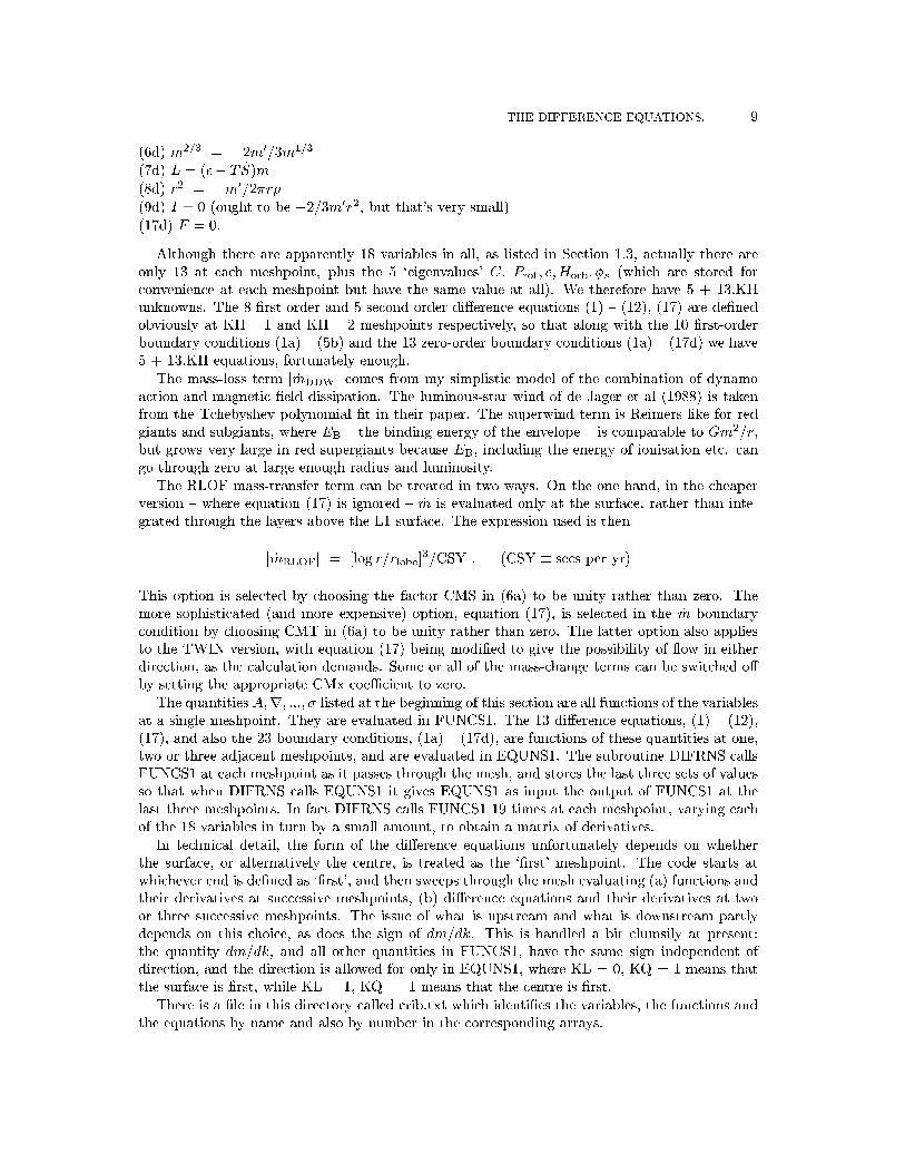
THE DIFFERENCE EQUATIONS. 9(6d) m2=3 = �2m0=3m1=3(7d) L = (�� T _S)m(8d) r2 = �m0=2�r�(9d) I = 0 (ought to be �2=3m0r2, but that's very small)(17d) F = 0.Although there are apparently 18 variables in all, as listed in Se tion 1.3, a tually there areonly 13 at ea h meshpoint, plus the 5 `eigenvalues' C, Prot; e;Horb; �s (whi h are stored for onvenien e at ea h meshpoint but have the same value at all). We therefore have 5 + 13.KHunknowns. The 8 �rst-order and 5 se ond-order di�eren e equations (1) { (12), (17) are de�nedobviously at KH { 1 and KH { 2 meshpoints respe tively, so that along with the 10 �rst-orderboundary onditions (1a) { (5b) and the 13 zero-order boundary onditions (1a) { (17d) we have5 + 13.KH equations, fortunately enough.The mass-loss term j _mDDWj omes from my simplisti model of the ombination of dynamoa tion and magneti �eld dissipation. The luminous-star wind of de Jager et al (1988) is takenfrom the T hebyshev polynomial �t in their paper. The superwind term is Reimers-like for redgiants and subgiants, where EB { the binding energy of the envelope { is omparable to Gm2=r,but grows very large in red supergiants be ause EB, in luding the energy of ionisation et . ango through zero at large enough radius and luminosity.The RLOF mass-transfer term an be treated in two ways. On the one hand, in the heaperversion { where equation (17) is ignored { _m is evaluated only at the surfa e, rather than inte-grated through the layers above the L1 surfa e. The expression used is thenj _mRLOFj = [log r=rlobe℄3=CSY : (CSY � se s per yr)This option is sele ted by hoosing the fa tor CMS in (6a) to be unity rather than zero. Themore sophisti ated (and more expensive) option, equation (17), is sele ted in the _m boundary ondition by hoosing CMT in (6a) to be unity rather than zero. The latter option also appliesto the TWIN version, with equation (17) being modi�ed to give the possibility of ow in eitherdire tion, as the al ulation demands. Some or all of the mass- hange terms an be swit hed o�by setting the appropriate CMx oeÆ ient to zero.The quantities A;r; :::; � listed at the beginning of this se tion are all fun tions of the variablesat a single meshpoint. They are evaluated in FUNCS1. The 13 di�eren e equations, (1) { (12),(17), and also the 23 boundary onditions, (1a) { (17d), are fun tions of these quantities at one,two or three adja ent meshpoints, and are evaluated in EQUNS1. The subroutine DIFRNS allsFUNCS1 at ea h meshpoint as it passes through the mesh, and stores the last three sets of valuesso that when DIFRNS alls EQUNS1 it gives EQUNS1 as input the output of FUNCS1 at thelast three meshpoints. In fa t DIFRNS alls FUNCS1 19 times at ea h meshpoint, varying ea hof the 18 variables in turn by a small amount, to obtain a matrix of derivatives.In te hni al detail, the form of the di�eren e equations unfortunately depends on whetherthe surfa e, or alternatively the entre, is treated as the `�rst' meshpoint. The ode starts atwhi hever end is de�ned as `�rst', and then sweeps through the mesh evaluating (a) fun tions andtheir derivatives at su essive meshpoints, (b) di�eren e equations and their derivatives at twoor three su essive meshpoints. The issue of what is upstream and what is downstream partlydepends on this hoi e, as does the sign of dm=dk. This is handled a bit lumsily at present:the quantity dm=dk, and all other quantities in FUNCS1, have the same sign independent ofdire tion, and the dire tion is allowed for only in EQUNS1, where KL = 0, KQ = 1 means thatthe surfa e is �rst, while KL = 1, KQ = -1 means that the entre is �rst.There is a �le in this dire tory alled rib.txt whi h identi�es the variables, the fun tions andthe equations by name and also by number in the orresponding arrays.

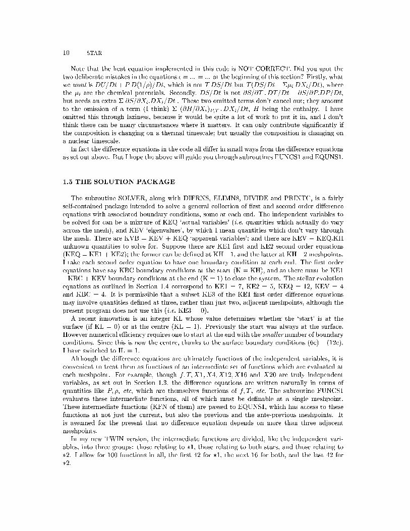
10 STARNote that the heat equation implemented in this ode is NOT CORRECT. Did you spot thetwo deliberate mistakes in the equations � = ... = ... at the beginning of this se tion? Firstly, whatwe want is DU=Dt+P D(1=�)=Dt, whi h is not T DS=Dt but T (DS=Dt+��iDXi=Dt), wherethe �i are the hemi al potentials. Se ondly, DS=Dt is not �S=�T :DT=Dt + �S=�P:DP=Dt,but needs an extra � �S=�Xi:DXi=Dt . These two omitted terms don't an el out; they amountto the omission of a term (I think) � (�H=�Xi)P;T :DXi=Dt, H being the enthalpy. I haveomitted this through laziness, be ause it would be quite a lot of work to put it in, and I don'tthink there an be many ir umstan es where it matters. It an only ontribute signi� antly ifthe omposition is hanging on a thermal times ale; but usually the omposition is hanging ona nu lear times ale.In fa t the di�eren e equations in the ode all di�er in small ways from the di�eren e equationsas set out above. But I hope the above will guide you through subroutines FUNCS1 and EQUNS1.1.5 THE SOLUTION PACKAGEThe subroutine SOLVER, along with DIFRNS, ELIMN8, DIVIDE and PRINTC, is a fairlyself- ontained pa kage intended to solve a general olle tion of �rst and se ond order di�eren eequations with asso iated boundary onditions, some at ea h end. The independent variables tobe solved for an be a mixture of KEQ `a tual variables' (i.e. quantities whi h a tually do varya ross the mesh), and KEV `eigenvalues', by whi h I mean quantities whi h don't vary throughthe mesh. There are KVB = KEV + KEQ `apparent variables'; and there are KEV + KEQ.KHunknown quantities to solve for. Suppose there are KE1 �rst and KE2 se ond order equations(KEQ = KE1 + KE2); the former an be de�ned at KH { 1, and the latter at KH { 2 meshpoints.I take ea h se ond order equation to have one boundary ondition at ea h end. The �rst orderequations have say KBC boundary onditions at the start (K = KH), and so there must be KE1{ KBC + KEV boundary onditions at the end (K = 1) to lose the system. The stellar evolutionequations as outlined in Se tion 1.4 orrespond to KE1 = 7, KE2 = 5, KEQ = 12, KEV = 4and KBC = 4. It is permissible that a subset KE3 of the KE1 �rst order di�eren e equationsmay involve quantities de�ned at three, rather than just two, adja ent meshpoints, although thepresent program does not use this (i.e. KE3 = 0).A re ent innovation is an integer KL whose value determines whether the `start' is at thesurfa e (if KL = 0) or at the entre (KL = 1). Previously the start was always at the surfa e.However numeri al eÆ ien y requires one to start at the end with the smaller number of boundary onditions. Sin e this is now the entre, thanks to the surfa e boundary onditions (6 ) { (12 ),I have swit hed to IL = 1.Although the di�eren e equations are ultimately fun tions of the independent variables, it is onvenient to treat them as fun tions of an intermediate set of fun tions whi h are evaluated atea h meshpoint. For example, though f; T;X1; X4; X12; X16 and X20 are truly independentvariables, as set out in Se tion 1.3, the di�eren e equations are written naturally in terms ofquantities like P; �, et , whi h are themselves fun tions of f; T , et . The subroutine FUNCS1evaluates these intermediate fun tions, all of whi h must be de�nable at a single meshpoint.These intermediate fun tions (KFN of them) are passed to EQUNS1, whi h has a ess to thesefun tions at not just the urrent, but also the previous and the ante-previous meshpoints. Itis assumed for the present that no di�eren e equation depends on more than three adja entmeshpoints.In my new TWIN version, the intermediate fun tions are divided, like the independent vari-ables, into three groups: those relating to �1, those relating to both stars, and those relating to�2. I allow for 100 fun tions in all, the �rst 42 for �1, the next 16 for both, and the last 42 for�2.

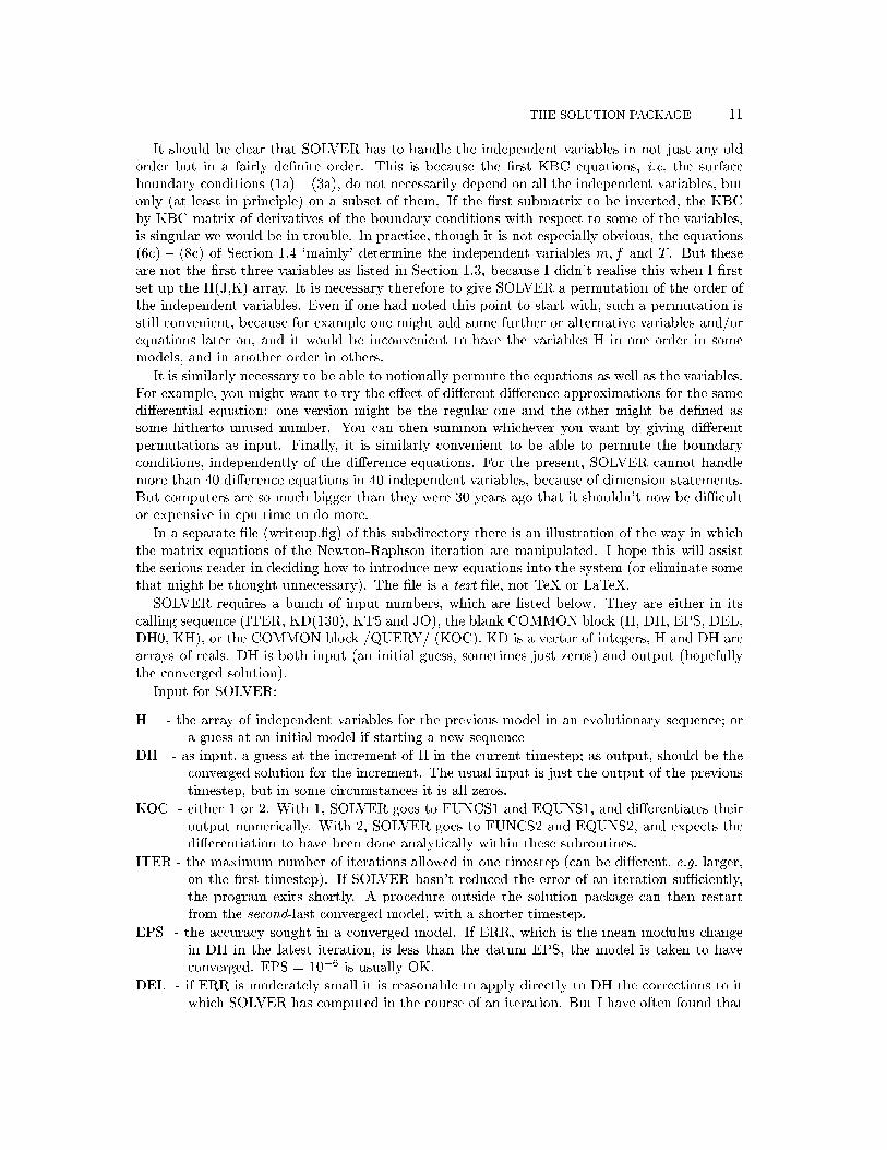
THE SOLUTION PACKAGE 11It should be lear that SOLVER has to handle the independent variables in not just any oldorder but in a fairly de�nite order. This is be ause the �rst KBC equations, i.e. the surfa eboundary onditions (1a) { (3a), do not ne essarily depend on all the independent variables, butonly (at least in prin iple) on a subset of them. If the �rst submatrix to be inverted, the KBCby KBC matrix of derivatives of the boundary onditions with respe t to some of the variables,is singular we would be in trouble. In pra ti e, though it is not espe ially obvious, the equations(6 ) { (8 ) of Se tion 1.4 `mainly' determine the independent variables m; f and T . But theseare not the �rst three variables as listed in Se tion 1.3, be ause I didn't realise this when I �rstset up the H(J,K) array. It is ne essary therefore to give SOLVER a permutation of the order ofthe independent variables. Even if one had noted this point to start with, su h a permutation isstill onvenient, be ause for example one might add some further or alternative variables and/orequations later on, and it would be in onvenient to have the variables H in one order in somemodels, and in another order in others.It is similarly ne essary to be able to notionally permute the equations as well as the variables.For example, you might want to try the e�e t of di�erent di�eren e approximations for the samedi�erential equation: one version might be the regular one and the other might be de�ned assome hitherto unused number. You an then summon whi hever you want by giving di�erentpermutations as input. Finally, it is similarly onvenient to be able to permute the boundary onditions, independently of the di�eren e equations. For the present, SOLVER annot handlemore than 40 di�eren e equations in 40 independent variables, be ause of dimension statements.But omputers are so mu h bigger than they were 30 years ago that it shouldn't now be diÆ ultor expensive in pu time to do more.In a separate �le (writeup.�g) of this subdire tory there is an illustration of the way in whi hthe matrix equations of the Newton-Raphson iteration are manipulated. I hope this will assistthe serious reader in de iding how to introdu e new equations into the system (or eliminate somethat might be thought unne essary). The �le is a text �le, not TeX or LaTeX.SOLVER requires a bun h of input numbers, whi h are listed below. They are either in its alling sequen e (ITER, KD(130), KT5 and JO), the blank COMMON blo k (H, DH, EPS, DEL,DH0, KH), or the COMMON blo k /QUERY/ (KOC). KD is a ve tor of integers, H and DH arearrays of reals. DH is both input (an initial guess, sometimes just zeros) and output (hopefullythe onverged solution).Input for SOLVER:H - the array of independent variables for the previous model in an evolutionary sequen e; ora guess at an initial model if starting a new sequen eDH - as input, a guess at the in rement of H in the urrent timestep; as output, should be the onverged solution for the in rement. The usual input is just the output of the previoustimestep, but in some ir umstan es it is all zeros.KOC - either 1 or 2. With 1, SOLVER goes to FUNCS1 and EQUNS1, and di�erentiates theiroutput numeri ally. With 2, SOLVER goes to FUNCS2 and EQUNS2, and expe ts thedi�erentiation to have been done analyti ally within these subroutines.ITER - the maximum number of iterations allowed in one timestep ( an be di�erent, e.g. larger,on the �rst timestep). If SOLVER hasn't redu ed the error of an iteration suÆ iently,the program exits shortly. A pro edure outside the solution pa kage an then restartfrom the se ond-last onverged model, with a shorter timestep.EPS - the a ura y sought in a onverged model. If ERR, whi h is the mean modulus hangein DH in the latest iteration, is less than the datum EPS, the model is taken to have onverged. EPS = 10�6 is usually OK.DEL - if ERR is moderately small it is reasonable to apply dire tly to DH the orre tions to itwhi h SOLVER has omputed in the ourse of an iteration. But I have often found that

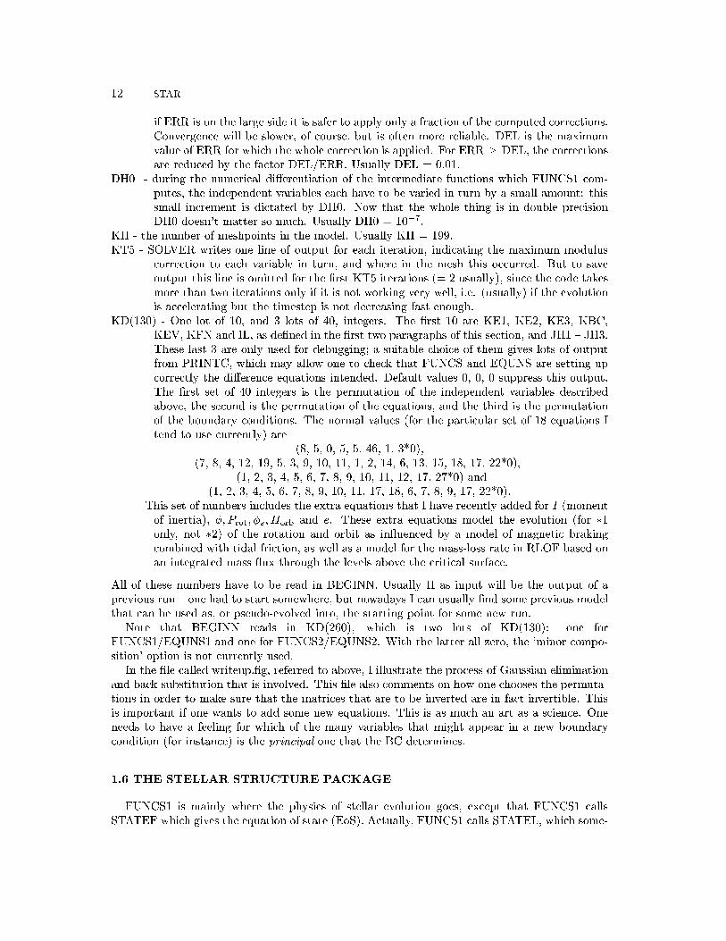
12 STARif ERR is on the large side it is safer to apply only a fra tion of the omputed orre tions.Convergen e will be slower, of ourse, but is often more reliable. DEL is the maximumvalue of ERR for whi h the whole orre tion is applied. For ERR > DEL, the orre tionsare redu ed by the fa tor DEL/ERR. Usually DEL = 0.01.DH0 - during the numeri al di�erentiation of the intermediate fun tions whi h FUNCS1 om-putes, the independent variables ea h have to be varied in turn by a small amount: thissmall in rement is di tated by DH0. Now that the whole thing is in double pre isionDH0 doesn't matter so mu h. Usually DH0 = 10�7.KH - the number of meshpoints in the model. Usually KH = 199.KT5 - SOLVER writes one line of output for ea h iteration, indi ating the maximum modulus orre tion to ea h variable in turn, and where in the mesh this o urred. But to saveoutput this line is omitted for the �rst KT5 iterations (= 2 usually), sin e the ode takesmore than two iterations only if it is not working very well, i.e. (usually) if the evolutionis a elerating but the timestep is not de reasing fast enough.KD(130) - One lot of 10, and 3 lots of 40, integers. The �rst 10 are KE1, KE2, KE3, KBC,KEV, KFN and IL, as de�ned in the �rst two paragraphs of this se tion, and JH1 { JH3.These last 3 are only used for debugging; a suitable hoi e of them gives lots of outputfrom PRINTC, whi h may allow one to he k that FUNCS and EQUNS are setting up orre tly the di�eren e equations intended. Default values 0, 0, 0 suppress this output.The �rst set of 40 integers is the permutation of the independent variables des ribedabove, the se ond is the permutation of the equations, and the third is the permutationof the boundary onditions. The normal values (for the parti ular set of 18 equations Itend to use urrently) are (8, 5, 0, 5, 5, 46, 1, 3*0),(7, 8, 4, 12, 19, 5, 3, 9, 10, 11, 1, 2, 14, 6, 13, 15, 18, 17, 22*0),(1, 2, 3, 4, 5, 6, 7, 8, 9, 10, 11, 12, 17, 27*0) and(1, 2, 3, 4, 5, 6, 7, 8, 9, 10, 11, 17, 18, 6, 7, 8, 9, 17, 22*0).This set of numbers in ludes the extra equations that I have re ently added for I (momentof inertia), �; Prot; �s; Horb and e. These extra equations model the evolution (for �1only, not �2) of the rotation and orbit as in uen ed by a model of magneti braking ombined with tidal fri tion, as well as a model for the mass-loss rate in RLOF based onan integrated mass ux through the levels above the riti al surfa e.All of these numbers have to be read in BEGINN. Usually H as input will be the output of aprevious run { one had to start somewhere, but nowadays I an usually �nd some previous modelthat an be used as, or pseudo-evolved into, the starting point for some new run.Note that BEGINN reads in KD(260), whi h is two lots of KD(130): one forFUNCS1/EQUNS1 and one for FUNCS2/EQUNS2. With the latter all zero, the `minor ompo-sition' option is not urrently used.In the �le alled writeup.�g, referred to above, I illustrate the pro ess of Gaussian eliminationand ba k-substitution that is involved. This �le also omments on how one hooses the permuta-tions in order to make sure that the matri es that are to be inverted are in fa t invertible. Thisis important if one wants to add some new equations. This is as mu h an art as a s ien e. Oneneeds to have a feeling for whi h of the many variables that might appear in a new boundary ondition (for instan e) is the prin ipal one that the BC determines.1.6 THE STELLAR STRUCTURE PACKAGEFUNCS1 is mainly where the physi s of stellar evolution goes, ex ept that FUNCS1 allsSTATEF whi h gives the equation of state (EoS). A tually, FUNCS1 alls STATEL, whi h some-

THE EQUATION-OF-STATE PACKAGE 13times alls STATEF. This is so that if you are in the pro ess of di�erentiating numeri ally wrtr, say, you don't have to reevaluate the EoS, whereas for log T , say, you do.FUNCS1 omputes the mixing-length approximation to the temperature gradient. It solves the ubi equation analyti ally, rather than approximately. FUNCS1 also sets up the minimal `rea -tion network', whi h only involves hydrogen burning via the pp hain and CNO bi- y le (with 3He,13C and 15N assumed in equilibrium, though not 14N and 16O), helium burning mainly by 3� and12C(�; )16O, and arbon, oxygen and neon burning just by 12C+12C, 16O+16O, 20Ne(�; )24Mgand a few related (�; ) and ( ; �) rea tions. This limited network results ultimately in a mixtureof 24Mg and 28Si (ex ept it doesn't often get there in pra ti e ....).Another of FUNCS1's ontributions is to evaluate the terms in the mesh-spa ing equation,i.e. in Q and Q0 (Se tion 1.4). Q is a tually a rather more sophisti ated fun tion than Se tion1.4 implies, but not vastly more. At the end of FUNCS1 the surfa e boundary onditions areevaluated (BC1 to BC7).FUNCS1 knows whether it is dealing with �1 or �2 of a binary by looking at JB, whi h is either1 or 2. For JB = 1 it omputes the evolution of rotation, e entri ity and orbital period a ordingto naive pres riptions for the ML rate of stellar wind, the AML rate be ause of magneti brakingin this wind, and the ex hange of angular momentum between the spin and the orbit be ause oftidal fri tion. The same pro esses in �2 are ignored. When JB = 2, FUNCS1 uses the alreadyknown mass-loss and mass-transfer history of �1 to provide a boundary ondition for �2.It would not be possible to determine the entire evolution of �1 before starting on that of �2unless we make the assumption that the only aspe t of �2 that in uen es �1 is �2's mass. It is notne essary that �1 evolve onservatively, sin e we an keep tra k separately of mass lost to in�nityby wind and mass lost to �2 by transfer. But we annot allow �2 to have its own wind-drivenmass loss, sin e that will depend, at the very least, on the luminosity, radius and rotation periodof �2 as well as its mass.The above has to be quali�ed if we are in the TWIN mode, solving both stars simultaneously.Then FUNCS1, at ea h meshpoint, does (a) things relating to �1 only, (b) things relating to �2only, and ( ) things that relate to both stars (e.g. heat transfer that depends on the di�eren ein enthalpies). This pro edure is rather omplex at the moment: I haven't had time to writesomething simple.1.7 THE EQUATION-OF-STATE PACKAGEThe EoS has an unusual form in that it gives su h quantities as P; �; CP; : : : as fun tions of thetwo independent variables f , a parameter related to ele tron degenera y, and T , the temperature.In addition. of ourse, the EoS depends on the abundan es of the various elements, whi h aregiven onstants for present purposes. The hoi e of f rather than say � or P as independentvariable is based on the fa t that several physi al pro esses, notably ele tron degenera y in oresand ionisation in envelopes, are expli it fun tions of f , but not of � or P . So also would be su hextra pro esses as pair produ tion and inverse �-de ay, although I have not a tually programmedthose. By using expli it formulae the omputation is rendered very eÆ ient; there is no needto invert a ompli ated highly non-linear relation � = �(f; T ) in order to determine the ele trondegenera y parameter f , whi h is needed in the Fermi-Dira integrals.Ele tron degenera y is normally represented as a quantity , whi h appears in su h Fermi-Dira integrals as Ne� = onst: Z 10 p2dpeEm 2=kT� + 1 :The quantities p;E are the dimensionless momentum and energy of an ele tron, related by E =p1 + p2�1; Ne is the number of free ele trons per a.m.u., whi h itself depends on via ionisation

14 STAR(see below). The quantity f gives expli itly, by de�nition, as = ln p1 + f � 1p1 + f + 1 + 2p1 + f ; so that d df = p1 + ff :

In terms of a further fun tion g(f; T ) de�ned by g = (kT=m 2)p1 + f , the Fermi-Dira integralabove an be approximated, to about 3 s.f. for all physi al f; T , byNe� = onst: f1 + f fg(1 + g)g3=2 P30P30 aijf igj(1 + f)3(1 + g)3 ;where the aij are a set of 16 onstant oeÆ ients found by least-squares. It is easy to see that infour limiting ir umstan es we have:f � 1 ; g� 1 : � lnf4 + 2 ; g � T ; Ne� = onst: 4a00T 3=2e �2

f � 1 ; g� 1 : � lnf4 + 2 ; g � T ; Ne� = onst: 4a03T 3e �2f � 1 ; g� 1 : � 2pf ; g � T2 ; Ne� = onst: a30( T )3=2f � 1 ; g� 1 : � 2pf ; g � T2 ; Ne� = onst: a33( T )3 :Similar approximations exist for the pressure and the internal energy U , or equivalently theentropy S, of the free ele trons. The oeÆ ients are to be found in the subroutine fdira .f.A se ond virtue of the above approximation is that, be ause it is losely based on the analyti expansions of the integral in its various limiting regimes, its partial derivatives, even up to thirdderivatives, are reasonably a urate, and an also be written down analyti ally. Sin e mu h ofthe physi s we need involves derivatives of P; S w.r.t. T; �, it is important that the derivativesare also a urate.Ionisation is expressed by a number of equations of the formNH+NH = !H+!H e +�H=kT ;where the !'s are statisti al weights and �H is the ionisation potential; this has to be solvedalong with NH+ +NH = X, where X is the given abundan e of hydrogen by mass. Obviouslythese two equations give both NH and NH+ simply and expli itly in terms of ; T or equivalentlyfor f; T . Similar equations (3 rather than 2) give the helium ionisation equilibrium. A slight ompli ation is that for hydrogen we also have to onsider the mole ular equilibrium, but it turnsout that this only means solving a quadrati rather than a linear equation for N(H).Two substantial problems remain, one of whi h is an artefa t of the hoi e f of independentvariable, and one of whi h is a problem however we hoose the independent variables. In order,(a) f or be omes indeterminate if the gas is fully non-ionised, so that there are no free ele trons,and (b) the ionisation equation above breaks down at high density (`pressure' ionisation), be ausethe atomi stru ture of ions is strongly modi�ed when the ions are so losely pa ked togetherthat their Bohr radii are less than their separation. I don't have an answer to (a), but mer ifullymost stellar material is hot enough, dense enough, or dilute enough, that at least some atoms

THE TIME-STEP PACKAGE 15are ionised. I help this along by approximating both Si and Fe as wholly ionised, even althoughthey are not.We deal with (b) approximately, by assuming that both the !'s and the �'s are dependenton Ne� and T , and only on these. Thus we add to the Helmholtz free enery a term of theform �F � NeF0(Ne�; T ). Then in the ionisation equation we have to add to the additional hemi al potential term (kT )�1(��F=�Ne)�;T . This works be ause (��F=�Ne)�;T , unlike �F , isa fun tion of Ne and � only through the ombination Ne�, and this in turn is a fun tion only of theinput variables f; T . We must also for thermodynami onsisten y add terms �2(��F=��)Ne;Tto the pressure and �(��F=�T )Ne;� to the entropy.1.8 THE TIME-STEP PACKAGEThe sele tion of the next timestep (in NEXTDT) is more of an art than a s ien e. This is atleast partly be ause all stellar models in assumed hydrostati equilibrium break down ultimately,approa hing either degenerate He ignition, degenerate C ignition, or a ore- ollapse supernova.But other less obvious pitfalls are ommonly en ountered before then. They ommonly requirethe timestep to be ut down drasti ally, but temporarily, and it is often diÆ ult to spot this inadvan e. Therefore the ode will sometimes fail to onverge; but it often re overs from this byretreating two timesteps and trying again with (say) half the timestep.Apart from a predi table breakdown at a late stage in evolution, one sometimes gets temporarybreakdowns at earlier stages. Mostly these are asso iated with one or other (or in tiresome asesmore than one) of the following:(i) Evolution a elerates rapidly at the end of ore-burning phases; sometimes DT isn't ut ba krapidly enough to ope.(ii) When a onve tive ore (or envelope) has a boundary moving into a formerly non- onve tiveregion, possibly with a omposition gradient, a omposition dis ontinuity is liable to buildup. This is physi ally OK, but may give the ode a problem. For the way a ompositiondis ontinuity propagates with an impli it di�usive treatment of onve tive mixing is by havingX (the abundan e) hange rapidly at one meshpoint while hardly hanging at all at bothadja ent meshpoints. Then when X has almost rea hed uniformity with the onve tive region,the same thing starts happening one point further out (or in). It is therefore diÆ ult toextrapolate reliably to the next model from the present and previous models, spe i� allywhen the rapid hange in X at one meshpoint is beginning to die out while that at the nextmeshpoint is beginning to pi k up. One might expe t that a short enough timestep would do it,and that is generally right; but the step has to shorten very rapidly at a rather unpredi tablepoint, and preferably also in rease again rather rapidly on e the diÆ ulty is (temporarily)over.(iii) On a line roughly oin iding with the blue edge of the Cepheid strip, the depth of the onve tive envelope is very sensitive to e�e tive temperature. The onve tive part of theenvelope may seek to expand or ontra t by 10 meshpoints in the ourse of a single timestep.The di�eren e equations are espe ially non-linear in this ir umstan e, and it is somewhatamazing that the Newton-Raphson te hnique (whi h assumes lo al near-linearity) works atall. In pra ti e it usually does, but sometimes it needs a temporarily shortened timestep.(iv) The onset of RLOF is similarly a very non-linear pro ess, on top of whi h the rate of evolution ommonly speeds up by a fa tor of � 100.The ode hooses the next DT on the basis of(a) ertain input numbers, viz. CDD, CT1, CT2(b) the DT you give it at the start of a run - normally the DT from the end of a previous run,but you an vary it

16 STAR( ) internally generated numbers: FAC � ��jDH(I;K)j/(KH*CDD), the ratio of the mean-modulus hange of the model in the timestep to a standard value (input CDD); and IHOLD(see below)(d) whether the model has onverged or not on its last timestep.Assuming onvergen e, for the moment, the ode tries to hoose DT su h that FAC is the same(unity) from one timestep to the next. So if the timestep DT just �nished gives a ertain FAC,the next timestep should be DT0 = DT/FAC. But to prevent DT from u tuating too rapidly(whi h often seems to ause numeri al problems), DT0/DT is restri ted to lie in the range (CT1,CT2), typi ally (0.9, 1.05), when things are running reasonably smoothly.When things are not running smoothly, the �rst symptom is that the number of iterationsneeded to rea h the required a ura y rises, from a typi al 2 to a permitted maximum of say12 (i.e. KTR2). Usually the timestep starts utting ba k, but often not fast enough. If even12 iterations fail to give onvergen e, the ode restarts from the anteprevious model, with DTde reased by a given fa tor CT3. Sometimes this is enough, and after 5 timesteps (determinedautomati ally by IHOLD), DT starts sele ting itself again. Sometimes the ode staggers on for afew timesteps, then fails again to onverge and restarts again, as above, with a further de reaseof DT. On o asion 5 su h restarts o ur before the ode pi ks up its usual rhythm. The worst ase is that the ode ontinues de reasing DT by further fa tors of CT3 without ever rea hing onvergen e, but DT is only allowed to de rease to 106 se s before the ode terminates.The following stratagem, to be done by hand rather than automati ally, an sometimes pushthe ode through some onvergen e failure (ex ept of ourse for the terminal diÆ ulties in the �rstparagraph of this Se tion). Retreat to the last stored model of the last run that went well, andevolve only so many timesteps that the ode terminates normally a few steps before the problem.Then halve (or quarter) DT manually, and prevent it from in reasing by putting CT1 = CT2 =1.0 (or maybe 0.95, 1.05). If it appears to be settling down after the diÆ ulty, remember to relaxCT1, CT2 a bit, or the al ulation may take forever.For �2 of a binary, the problem is ompounded. The same DT as �1 will seldom do, sin e atan early stage �2 may be evolving more slowly than �1 and at a later stage faster. Also, oneor other star may need to a elerate strongly, while the other does not. NEXTDT knows �1'stimestep history while trying to de ide on �2's next timestep. Mainly it operates in the sameway as for �1 (above), while looking for the timesteps in �1 that in lude the beginning and theend of �2's timestep; but if this would en ompass a large number of timesteps of �1 the timestepfor �2 is ut ba k a bit.The pro ess for �2 works least well early in RLOF, where the mass-transfer rate grows rapidlyfrom zero to the thermal times ale. The ode at present never quite redu es the timestep of �2to what I would like: typi ally there are half-a-dozen timesteps that are about twi e the size thatwould be desirable. Somewhat surprisingly the ode seems to onverge without diÆ ulty, but �2 hanges more in one timestep than one would wish on the grounds of a ura y. This seems tobe be ause (a) the thermal times ale of �2 at this point is usually quite a lot shorter than �1's,and (b) the rate of mass gain of �2 is obtained from linear interpolation in �1's history, and sois in e�e t onstant for a while and then in reases as a step-fun tion. Perhaps I need non-linearinterpolation, but sin e the variation of _m in �1 is itself a very rapid a eleration, non-linearinterpolation would seem even more problemati than linear.A further ompli ation, though apparently not a major one, is that in the interest of e onomythe ode ip- ops between �1 and �2, doing say 200 steps of the �rst and then enough steps ofthe se ond to at h up. Without this, �1 might be evolved to a pre-supernova, only to dis overthat �2 ame into onta t with �1 while �1 was still in the main-sequen e band.

THE INPUT AND OUTPUT DATA 171.9 THE INPUT AND OUTPUT DATAThe following data numbers all have to be assigned. Some are never, or very seldom, hanged;some are hanged in order to spe ify what kind of evolutionary run you want; and some haveto be hanged, or are hanged automati ally, in response to way the run is progressing. It isof ourse something of an art form to ome up with hanges that allow you to ope with someunpredi ted breakdown. There are a few numbers whose hoi e seems fairly deli ate for gettingthe thing to run smoothly. They mostly have to do with hoosing the best timestep, and theway that timestep should in rease or de rease in response to the evolution. Some rules of thumbwere given in the previous Se tion. The values whi h I usually assign are given below in bra kets(ex ept for long ve tors).I �nd it simplest to use the default names fort.n (on some omputers ftn0n) for the �le thatis read or written to unit n. Files 1 { 3, 8, 9, 13 { 15 are used as output, �les 16 { 21 are used as(relatively) �xed input, �le 22 is hanged o asionally, and only �le 23 is normally hanged fromjob to job, de�ning what parti ular masses and period are required. Starting with �les 13 { 21,in reverse order, and �nishing with �les 22 and 23:..............................Fort.21 ontains data for onverting from L; Te to MV; B � V; U �B, and some nu lear data(Q-values for nu lear rea tions and neutrinos, numbers for omputing s reening orre tions) andatomi data (ionisation potentials, statisti al weights, atomi masses and numbers)...............................Fort.20 ontains the OPAL opa ity data, ombined with mole ular opa ities, and it also on-tains nu lear rea tion rate data and neutrino loss rates:KCSX : The number of di�erent sub- ompositions tabulated, � 10, urrently 8 or 9CZS : the metalli ityCH : the initial hydrogen mass fra tion, whi h I usually take to orrelate with CZS, CH = 0.76{ 3*CZSCSX(10) : Numbers whi h des ribe indire tly the 8, 9 or 10 sub- ompositionsCS(90,127,10) : The opa ity tablesCHAT(8920) : Neutrino loss rate and nu lear rea tion rate tables..............................Fort.19 ontains just 4 numbers, MLO, DM, MHI, KDM, de�ning the masses of the modelsstored in fort.16 and fort.17 below. The present numbers say that the ZAMS models providedin fort.18 have log masses ranging from MLO = { 1.00 to MHI = 2.30 in lusive, in steps of� log10M = 0:025; and that the orresponding summary in fort.17 is KDM = 5 times more�nely spa ed. .............................Fort.18 ontains a short summary of every fourth model in a run (exe uted previously) wherethe mass in reases from 0.1 to 200M� in equal in rements of log10M . For every twentiethmodel there are also interior details like log �; log T; logP; : : :. The �le was output (on fort.1) ofa previous job. .............................Fort.17 ontains a `pruned' version of fort.18, with just 5 lines for every fourth model. Thepruning is done automati ally at the start of ea h job; so fort.17 is not a tually needed as data..............................Fort.16 ontains the interior details of every twentieth ZAMS model on fort.18, in the formneeded to start a new run (whi h is di�erent from the form to be seen in fort.18). These areouput from the same previous run, pseudo-evolving a star that gained mass yet didn't evolve(mu h), i.e. a ZAMS run. More on this later. But the output �le of one run is suitable to bethe input �le of another run. The 133 ZAMS models on fort.16 have to orrespond of ourse to

18 STARthe metalli ity of the opa ity table of fort.20. There is no marker between one model and thenext, but the �rst line of ea h model says how many following lines belong to it. In fa t they allhave 199 grid-points, and so 200 lines when we in lude the �rst line. The �rst line, whi h onesometimes edits by hand { but whi h one an also supersede by putting some repla ent numbersin fort.23 { ontains the following:SM : The stellar mass, in solar units. All of SM { ENC below an be re-initialised by data infort.23.DTY : The next time-step, in years.AGE : The age, in years.PER : The orbital period, in days. For a single star, take say 1.0d10BMS : The total mass of the binary. The star you are evolving is always in a binary, but you an make the binary so wide (using PER above) that it is e�e tively single. BMS may hange with time if stellar-wind mass loss from �1 is in luded.ECC : The orbital e entri ity; will go to zero if tidal fri tion is in luded, and if the binary is lose enough.P1 : The rotational period of the star, whi h approa hes syn hronism with the orbital period iftidal fri tion is in luded.ENC : A onstant (in spa e, but not in time) energy generation rate that an be added to theusual nu lear term, for onstru ting Hayashi-tra k pre-MS stars from ZAMS stars. SeeCEA, CET below (fort.22). ENC is the starting value for the run, and it is made toin rease, on a times ale 1/CET (yrs) towards an asymptoti value CEA (ergs/gm/se ).(0.0)KH : The number of mesh-points in the input model to be read in shortly.KP : The number of time-steps you want to take.JMOD : The number of time-steps it has already taken. If starting from the ZAMS, you anreset JMOD = 0, and in the �rst step nu lear and thermal evolution are ignored, whi h an be useful.JB : For JB = 1, the star is treated as the primary of a lose binary, and will lose mass whenit �lls its Ro he. For JB = 2, it is the se ondary. The ode runs the primary �rst,and then puts its output through a subsidiary (very simple) programme alled pruner.f,whi h produ es a �le ontaining mass as a funtion of time. With JB = 2, the se ondaryuses this �le to gain mass at the appropriate rate as a fun tion of time. What happenswhen the se ondary also �lls its Ro he lobe? If you �nd out, let me know. In the latest ode, the swit h from �1 to �2 is handled automati ally, and an happen every (say) 100timesteps of �1. Thus if �2 �lls its Ro he lobe fairly early on, we haven't wasted timeevolving �1 to a supernova.JIN : The number of independent variables of the H, DH arrays to be read in. This may bein reased early in the run by adding in some estimates for extra variables satisfying extraequations. I do this in REMESH, whi h is alled on e only, almost at the beginning ofa run. JIN may therefore be hanged in REMESH. (11, 16)H(40,500) : The details of an initial model, normally an output model of a previous run. You an use as many as 499 meshpoints (not 500, for some reason), but mostly I have stu kwith 199.Although the models in fort.16 have spe i� values of SM, ... JMOD, these an be supersededby values you sele t in fort.23 below.........................................Fort.13 { fort.15 optionally ontain similar models whi h an be read in as data (a ordingto what one puts in fort.23), and whi h were output from previous runs. As output, fort.15 ontains every NSV'th model (or pair of models, for a binary) omputed in a run; fort.13 andfort.14 ontain the last and the se ond last model that were stored. The ode alternates between

THE INPUT AND OUTPUT DATA 19them, overwriting anything previous, so it is not ne essarily lear whi h is the last and whi h these ond last without looking at their �rst lines..........................................Fort.22 and fort.23 are ` on�guration �les', determining the kind of job to be done. Fort.22 iso asionally hanged, and fort.23 usually hanged, from one run to another. The following areread from fort.22, in subroutine BEGINN. There are 25 rows, but doubled (for binaries) sin ethe �rst lot applies to �1 of a binary and the se ond, whi h may be di�erent, to �2.First row:KH2 : The number of mesh-points you want; if this di�ers from KH (above) the ode shouldinterpolate in the given model to produ e a new one; but you must also set JCH (below)to � 2 to implement this hange (199)KTR1 : The maximum number of iterations allowed on the �rst timestep (12)KTR2 : The maximum number of iterations allowed on later timesteps (12)JCH : If JCH = 2, 3 or 4, the ode (in REMESH) initialises the model in various ways, e.g.by using a new mesh-point distribution fun tion, so that the new model is to be got byinterpolation in an old model. For a ZAMS model, you an initialise to a given uniformX(1H), ... X(16H) by taking JCH = 4. You an also hange the mass, preferably by justa small amount, with JCH> 2. (1, 2, 3 or 4)KTH(1) { (4), alias KTH { KZ:KTH : �th = KTH � (T DS/Dt); so you an ignore T DS/Dt if you want (1 or 0)KX : DX(1H)/Dt = KX � (burning rate of 1H); so you an ignore the omposition hange whilekeeping the energy produ tion (1 or 0)KY : The same, for 4He (1 or 0)KZ : The same, for 12C and 16O (1 or 0)Se ond row:KCL(1) { (7), alias KCL, KION, KAM, KOP, KCC, KNUC, KCN:KCL : Default unity in ludes the Coulomb orre tion to pressure et . Zero suppresses it. (1)KION : EoS does the ionisation of the �rst KION elements in the list H, He, C, N, O, Ne, Mg,Si, Fe. No other elements are in luded. KION = 5 is about optimal. Don't try 9. (5)KAM : Not urrently usedKOP : If 1, ode should use spline interpolation in tables of opa ity; if 0, simple bilinearinterpolation (1)KCC : Not urrently usedKNUC : Not urrently usedKCN : If 0, gives standard nu lear network. If 1, gives a CNO equilibrium fudge for ZAMSmodels: see FUNCS1 (0)Third row:KT(1) { (4), alias KT1, KT2, KT3, KT4:KT1 : Print internal details of every KT1'th model (20 or n200)KT2 : Print internal details at every KT2'th meshpoint of the KT1'th model (1 or 2)KT3 : Print KT3 `pages' of details for every KT1'th model (1, 2 or 3)KT4 : Print a �ve-line summary of every KT4'th model (1, 2 or 4)KT5 : Print a one-line summary of ea h iteration of ea h model, ex ept for the �rst KT5 iterationsof ea h model (0 or 2)KSV: an output model is stored in fort.15 after every KSV'th timestep in a run, in the formneeded as input for a further run. The last model of a run is automati ally also stored,in fort.13 or fort.14. (5000)Fourth row:EP(1) { (3), alias EPS, DEL, DH0:

20 STAREPS : The a ura y to whi h SOLVER is expe ted to solve the equations (10�6)DEL : See se tion 1.5 (10�2)DH0 : See se tion 1.5 (10�7)CDD : The mean in rement, r.m.s.-wise, that you would like in one timestep (.01)Next 14 rows:KD(260) : See se tion 1.5Next 3 rows:KSX(45) : The �rst 15 integers identify the quantities, su h as log �; L;X(4He) ... , whi h areto be printed in olumns on the �rst `page' of stru ture details for every KT1'th model(see above). The next two lots of 15 relate to the optional further `pages'. The variablesare: 1 - , 2 - P, 3 - �, 4 - T, 5 - �, 6 - ra, 7 - r, 8 - rr �ra, 9 - m, 10 - H1, 11 - He4,12 - C12, 13 - N14, 14 - O16, 15 - Ne20, 16 - Mg24, 17 - r, 18 - L, 19 - �th, 20 - �nu ,21 - �� , 22 - Æm, 23 - not used, 24 - n=n + 1 = d log �=d log p, 25 - d log r=d logP , 26 -d logm=d logP , 27 - U (int. en.) , 28 - S, 29 L=LEdd, 30 - w onvl, 31 - �, 32 - wt, 33 - �e,34 - �e0, 35 - w onv, 36 - I, 37 - �, 38 - Fm, 39, 40, 41 - not used, 42 - �L, 43 - �(enth.),44 - v2, 45 - fa .Row 22:CT1 : The next timestep annot (normally) be less than CT1 times present timestep (0.8, 0.9or 1.0)CT2 : The next timestep annot be greater than CT2 times present timestep. If both CT1 andCT2 are 1.0, then the timestep is onstant, of ourse (whi h is useful for onstru ting aZAMS by arti� ial `mass-gain') { ex ept that if a model fails to onverge the timestepwill be multiplied by CT3 (next) (1.1, 1.05 or 1.0)CT3 : when the solution pa kage fails to onverge, the ode retreats to the se ond-last onvergedmodel, and ontinues with the timestep de reased by the fa tor CT3. (0.3 or 0.5)CT(1) { (10): oeÆ ients used in the mesh-spa ing fun tion QRow 23:CC, CN, CO, CNE, CMG, CSI, CFE : values for initialising X(12C), ... X(56Fe), as fra tions ofthe total metalli ity Z (= CZS, above); only used for ZAMS models, with JCH (above)= 4 (0.176, .052, 0.502, 0.092, 0.034, 0.072, 0.072)Row 24:CALP : The mixing-length ratio (2.0)CU : Along with COS and CPS (next), a ` onve tive overshoot' parameter; see CRD below (0.1)COS : A onve tive overshoot parameter for H-burning ores; see CRD below. Zero implies noovershoot. (0.12)CPS : as COS, but for He-burning ores: tri ky, COS(He) = COS(H) * CPS (1.0)CRD : The di�usion oeÆ ient � for onve tive mixing is taken to be CRD times the `legiti-mate' rate from mixing-length theory, ex ept that an approximate fa tor [rr �ra℄1=3is repla ed by [rr �ra +rOS℄2, whererOS � COS(2:5 + 20�� + 16�2�) (CU : � logm=� logP + 1) ; �� � PradPgas :The usual CRD is 10�2.CXB : De�nes the boundary of a ore to be at X(1H) or X(4He) = CXB (0.15)CGR : De�nes the boundary between a onve tion zone and a semi onve tion zone, for printoutpurposes only, to be at rr �ra = CGR (0.01)CEA : A onstant energy rate ENC (fort.18 above) an be added to �nu + �th� �� . An in reasingENC an push a star ba k from the ZAMS to the Hayashi tra k. CEA and CET (next)determine how ENC hanges with time (1.0E2)

THE INPUT AND OUTPUT DATA 21CET : See CEA above. The equation for the growth of ENC with time is dENC=dt =ENC.CET.(1 { ENC/CEA), so that ENC in reases exponentially on the assignedtimes ale 1/CET (yr), until saturating at ENC � CEA. (1.0E-6)Row 25 (last row):CMS : At the surfa e, _m = { CMS� [log r=rlobe)℄3 { CMT*F + CMI�m { CMR�1:3E � 5 � L �m=jEBEj { CMJ� _MJNH { CML��(L; r;m; Prot); so you an in lude if you like one of twoversions of mass transfer by RLOF (CMS, CMT), a onstant mass-gain/loss rate, mainlyfor running up or down the ZAMS (CMI), a Reimers-like mass-loss rate (CMR), a mass-loss rate for luminous stars (de Jager, Nieuwenhuizen & van der Hu ht 1988; CMJ), anda mass-loss rate as obtained from a simplisti dynamo theory (CML). Units are: CMT(M�=yr), CMI (yr�1), CMR, CMJ, CML (dimensionless). Remember what [: : :℄ means(p7). (0.0, or 1.0D4)CMT : See CMS above (0.0, or 1.0D-2)CMI : See CMS above (0.0, � 5.0D-9 or �1.0D-6)CMR : See CMS above (0.0 or 0.2 or 1.0)CMJ : See CMS above (0.0 or 1.0)CML : See CMS above (0.0 or 1.0)CHL : A fa tor multiplying the rate of ang. mom. loss asso iated with the rate of mass loss �,a ording to the same dynamo model. (0.0 or 1.0)CTF : A fa tor multiplying an expression for the rate of tidal fri tion. (0.0 or 0.01)CLT : A oeÆ ient used in the estimation of heat ux between omponents in onta t. It doesn'treally work yet.In Se tion 1.4 two options for mass transfer in binaries were des ribed. The above des riptionapplies only to the �rst of them. .........................................Fort.23 is eight rows with various ontrol numbers. You have to de ide on ea h of three options,ea h giving two alternatives. The options are(a) single stars or binary stars(b) new, ie starting from s rat h (ZAMS), or old, eg starting from the end model of a previousrun.( ) independent evolution, or simultaneous evolution, of the omponents.Not all 8 possibilities make sense: if you are doing simultaneous evolution, you won't want singlestars. The remaining possibilities should be viable.You also have to de ide whether you want a `one-shot' or `grid' run. A grid means severalruns, one after the other (but simultaneous using the massively parallel version, not des ribedhere), with the three parameters of primary mass, mass ratio and orbital period being y ledthrough. One-shot means what it says. On e again, some ombinations of this with the previous hoi es don't make sense, but most of them do.The �rst row is integers ISB, KTW, IOP1, IM1, IOP2, IM2, KPT, KP:ISB: single or binary. ISB = 1 implies only single stars to be omputed; ISB = 2 gives binaries.For single stars, you may still use the outer (�rst) y le for masses. The inner 2 y les shouldbe set to do only one ase ea h. The mass ratio and the period are of ourse virtually ignored,but have to be supplied. The period should be so large that there is no danger of RLOF (e.g.XL = 7.0, meaning a period of � 107 d).KTW: 1 for normal operation; 2 for TWIN mode, where both stars are solved simultaneously.IOP1: the number (13 { 16) of the �le (fort.13 { fort.16) where the initial model for �1 is to betaken from. ZAMS models are on fort.16.IM1: the sequential number of the model required on fort.IOP1. This is omputed automati ally,from later data, if the ZAMS �le fort.16 is used, so that if IOP1 is 16, it doesn't matter whatvalue you give for IM1, but you have to give a value.

22 STARIOP2: as IOP1, but for �2.IM2: as IM1, but for �2.KPT, KP: KPT is the maximum number of timesteps for ea h omponent (2000 to 4000 for fairly omplete evolution). Do approximately KP of �1, then enough of �2 to at h up with �1,then another � KP of �1, et , so that if �2 breaks down before �1 you don't waste a lot of al ulation on �1. You will seldom get exa tly the number of timesteps that you ask for. Forsingle stars, KP is set to KPT automati ally.The next 3 rows are parameters for 3 nested loops (mass, mass ratio, and initial period) to berun through: starting value; in rement; number of ases (1 more than the number of in rements).The �rst loop is: log10 (mass, solar units), starting at ML1, in reasing by steps of DML to ML1+ (KML { 1) . DMLThe se ond loop is: log10 (mass ratio in sense flarger/smallerg), starting at QL1, in reasing bysteps of DQL to QL1 + (KQL { 1) . DQLThe third loop is: X � log10(orbital period /period ne essary for *1 to �ll its Ro he lobe whenstill on the ZAMS), starting at XL1, in reasing by steps of DXL to XL1 + (KXL { 1) . DXL.Obviously you an arrange for only one model (single or binary) to be done, by taking KML =KQL = KXL = 1.The next (�fth) row isROT = rotational period of �1 / rotational breakup period.The sixth row is eight numbers AX(8), and an integer JMX. The AX's are optional repla e-ments for the values of SM, DTY, ... , ENC that the ode would normally pi k up in fort.IOP1from some previous run, or from the ZAMS library (fort.16 above). JMX similarly is an optionalrepla ement for JMOD. They are only applied if they are non-negative. Thus you an repla eonly one, or several.The obje t of the optional repla ement is this. Suppose you want to model a parti ular binary,and believe starting values (1:8 + 1:6M�; 3 d) will do. The nearest (log) masses in the libraryare 0.25 and 0.20, so set the M and Q loops a ordingly (ML1 = 0.25, QL1 = 0.05, with KML =KQL = 1). But then in the sixth row put SM = 1.8, BM = 3.4 (binary mass). You won't knowwhat X orresponds to 3 d, so also put PER = 3.0 in the sixth row. You an set the rotationalperiod also (P1): the same for both omponents, I'm afraid. There are omplexities here that Iprobably won't resolve till I retire; eg. in some operational modes one doesn't follow the rotationof the star, only the orbit; or you might follow the rotation of �1 but not �2. Don't give a short(<� 106 d) rotational period unless you are omputing the rotational evolution, sin e the star willkeep rotating at the same rate for all time and perhaps be ome rotationally unstable as a redsupergiant.The last two lines are a set of riteria to determine when the run is to be ended, eg. whenthe age is greater than 2 � 1010 yr. You'll have to read the end of printb.f to �gure them out.........................................Fort.13 and fort.14 are used by the ode for storage of intermediate or �nal models (in the sameformat as the input models of fort.16 above). This an be used for ontinuing a run with a furtherrun. The ma hine alternates between 13 and 14, overwriting previous models. You therefore havea ess only to the last two stored models. It may not be lear till you look inside them whi ha tually has the last model, although the one-line output on fort.8 ontains the relevant IOP, aswell as the termination ode (see below) and a few other numbers.In addition to getting the last model of a run on fort.13/14, the parameter KSV in fort.22 saysthat the ode stores every KSV'th timestep in fort.15. I usually don't bother, and take KSV =5000, whi h is more than most runs take.........................................The major useful output of a run omes out on fort.1, for �1 of a binary or for a single star,and on fort.2 as well if binary. This output has the same format as the input �le fort.17. After

MODES OF OPERATION, AND BREAKDOWN 23�1 has �nished, fort.1 is `pruned' down and put in fort.3, where it serves as input for the nextpart of the evolution of �2: �2 has to know the mass-loss and angular-momentum-loss history of�1 in order to a rete mass at the right rate.After a binary run is ompleted, the fort.2 output of �2 is also pruned down. Then fort.9 is reated whi h is �rst fort.3 (the pruned version of �1's run) and then the pruned-down versionof fort.2. Fort.9 is output whi h I often send to a plotting routine to look at.The ode reates a tiny fort.8, a single line (per run) with integers identifying how the �1 and�2 runs ended (impending SNEX, lifetime > 20Gyr, et ). These termination odes are listed inthe next Se tion (and also at the beginning of fort.8). If several runs are done in a loop, theya umulate in fort.8 and fort.9 (and fort.15, if used), but the other output �les are overwritten.1.10 MODES OF OPERATION, AND BREAKDOWNThe usual mode is `legitimate' evolution, say starting from the ZAMS and ontinuing till the ode �nally breaks down at the He ash, or degenerate C ignition, or a bit beyond non-degenerateC ignition. For binaries, there are some other ways to break down. A parameter JO indi atesroughly why a run stopped: for a binary there would be one value for ea h star. The JO valuesare:-1 { STAR12 { no timesteps required0 { STAR12 { �nished required tsteps OK1 { SOLVER { failed; ba kup, shorten tstep2 { BACKUP { tstep redu ed below limit; quit3 { NEXTDT { �2 evolving beyond last �1 model4 { PRINTB { �1 rstar ex eeds rlobe by limit5 { PRINTB { age greater than limit6 { PRINTB { C-burning ex eeds limit (i.e. lose to SNEX)7 { PRINTB { �2 rstar ex eeds rlobe by limit (i.e. onta t, or reverse RLOF)8 { PRINTB { lose to He ash9 { PRINTB { massive (> 1:2M�) degenerate C/O ore10 { PRINTB { j _M1j ex eeds limit11 { NEXTDT { impermissible FDT for �212, 22, 32 { as 2, but with non-zero entral H, zero entral H and non-zero entral He, and zero entral H and entral He, respe tively.JO = 32 is mu h the same as JO = 6, indi ating that a supernova explosion is imminent.If you want to evolve a star up to some parti ular point, say where entral H is 0.05, and thenstop, the simplest way is to put an extra JO ode in printb.f, along with the others there:IF ( DABS(DMT).GT.30.0D0*PX(9)/TKH) JO = 10 ! already thereif ( sx(10,1).lt.0.05d0 ) jo = 13 ! new line.I'm afraid it is not very transparent that sx(10,1) is the entral hydrogen abundan e. SX storesup to 45 variables at ea h meshpoint: a DATA statement near the start of printb.f identi�es them(not all are used).But as well as doing legitimate evolution, one an also do pseudo-evolution: moving the starup or down the main sequen e by adding or subtra ting mass while not allowing the ompositionto hange; generating a low-mass HB star from a high-mass one (thus avoiding the He ash) bylosing surfa e mass, but allowing the hydrogen shell to burn outwards while preventing entralhelium from burning; generating a pre-main sequen e Hayashi-tra k star from a ZAMS model byputting a uniform arti� ial energy sour e in the star; generating a white dwarf sequen e; et .The input data �le fort.22 above has entries that determine what kind of run is to be done.For example, you an move up or down the MS by setting CMI (� d lnm�=dt) in fort.22 to (say)

24 STAR�5:10�9 (yr�1) instead of zero. With DTY = 5:73992:105, this means that the mass is multipliedby 10 in the ourse of 800 timesteps. Prevent DTY from varying during evolution by puttingCT1 = CT2 = 1 in fort.22. Choose the right number of steps (KPT) to get you to where youwant. The �nal output model will be put in fort.13 (or 14), and intermediate models at everyKSV'th timestep are stored in fort.15. If you are `evolving' through the region � 1� 2M�, youmay need smaller timesteps, sin e the onve tive boundaries tend to move rather rapidly in thisregion. DTY, and also KPT, are fed in by fort.23 rather than fort.22.Note that we have two de�nitions of `ZAMS', both idiosyn rati . In one the star has anabsolutely uniform omposition in 1H, 4He, 12C, 14N, 16O, 20Ne, 24Mg, 28Si and 56Fe. Sin e 12Cburns very rapidly to 14N in moderate to high mass stars, evolution from this `ZAMS' modelstarts with a jerk (unless you use a very small timestep). A reasonable ploy is to begin by takinga single timestep of `normal' length, i.e. about 0.002 - 0.005 times the expe ted lifetime in theMS band. This will, if it works at all, relax the C/N into equilibrium, for those upper MS modelswhere pp is not the dominant energy sour e.In the se ond de�nition, 12C/14N equilibrium of a sort is obtained, with a uniform distributionof all the other spe ies, by solving for the C abundan e only. The best ZAMS is likely tobe obtained by (a) going down the MS with a ompletely uniform omposition and with the omposition hange (and the thermal energy term) suppressed, to get a star of say 0.08 or 0.1M�; and then (b) go up, allowing the C/N to equilibrate (KCN = 1) but otherwise suppressing omposition hanges. Throw away the (a) ZAMS, and keep the (b) one. The point about theparti ular values suggested for CMI and DTY is that one evolves through the region 1 � 2M�on something like a thermal times ale, whi h is also about the times ale on whi h a tual starsget there from the Hayashi tra k.From a ZAMS model with CN equilibrium one an generally evolve very easily to the He ash(in low-mass stars), degenerate C ignition (intermediate-mass stars), or the end of C burning(massive stars). One an let it run entirely automati ally, taking � 2000 � 3000 timesteps, orif one is prepared to intervene a bit one an do it in only 1000 timesteps. `Intervention' meansvarying CDD from one portion of run to the next. A value like 0.01 is OK on the MS, but maybeshould be less for entral He burning, and more for steady shell burning, whether single or doubleshell. The value of 0.01 seems to work all the way, with the ode having to ba ktra k and halvethe timestep, maybe more than on e, in some diÆ ult regions, and with somewhat unne essarilyslow progress in shell burning.The problem of the He ash is diÆ ult, be ause an impli it entrally di�eren ed s heme appearsto be unstable, generating saw-tooth os illations, on e a part of the star starts to evolve on amu h more rapid than thermal times ale. The problem is possibly ompounded by my adaptivemesh, although I have no eviden e that it is either worse or better than with a �xed mesh. Adi�erent form of di�eren ing is probably required if one wants to follow the ash in detail { andI suspe t one ought to do it in 3-D, not 1-D. I have not persevered with the He ash in 1-Dbe ause one an easily onstru t `post-He- ash' models by a roundabout route:(1) Evolve a ZAMS 2.5M� model till its entral He has just ignited (non-degenerately, by awhisker). Use KY = 0, so that although the He burns (ie. provides energy) it is not onsumed.(2) Subje t it to fairly rapid mass loss, using a negative CMI, but preventing this from ontribut-ing thermal energy (KTH = 0) till the surfa e mass is down to what you want.(3) Finally swit h o� the mass loss, and let the shell burn outwards till it rea hes the ore massyou want, while ontinuing to suppress the He evolution in the ore (KY = 0).With a bit of pra ti e one an produ e by similar stratagems(a) `ZAHeMS' stars(b) He, or C/O, white dwarfs( ) pre-MS fully onve tive (i.e. Hayashi tra k) stars.

MODES OF OPERATION, AND BREAKDOWN 25In some ases, one might edit the input model by hand, say moving the H-shell in or out by ameshpoint, or even removing it altogether if it is fairly near the surfa e and you don't want it.The parameter ENC an be used to onstru t pre-MS Hayashi tra k stars, from ZAMS ones.ENC is a onstant energy sour e ( onstant in spa e, not time), normally zero. Make it non-zeroand in rease it gradually (at rate CET), keeping KTH = KX = 0, so that the star swells up andits entre ools down. ENC an also be used to make luminous `zero-age' white dwarfs.It is possible to remove the omposition equations altogether from the solution step, so that the omposition remains �xed at ea h meshpoint even although the mass will vary at ea h meshpointbe ause of the adaptive grid. To do this you need di�erent values for the integers KD(1) -KD(130) in fort.22, viz. (grouping in 10 and 3 lots of 40): (5, 0, 0, 3, 1, 18, 0, 0, 0, 0), (1, 2,4, 8, 7, 6, 34*0), (6, 7, 8, 9, 10, 35*0), (6, 7, 8, 6, 7, 8, 34*0). This would allow you to redu ethe ore mass of an HB star while simultaneously redu ing its total mass, not ne essarily at thesame rate. I hope this also illustrates the intended exibility of the solution pa kage: you anadd in extra di�erential equations that you want solved along with the stru ture, but you analso easily ignore them in ir umstan es where you temporarily don't need them.The programme an handle semideta hed binaries rather easily, on the assumption that �1,the more massive star initially, �lls its Ro he lobe �rst, and that �2 never �lls its Ro he lobe.A tually, there is plenty of opportunity for �2 to �ll its own lobe. It is pretty well bound to, ata late stage when �1 has �nished its evolution and be omes an NS or WD. But it may well �llit before then, parti ularly while �1 still is semideta hed, so that the stars ome into onta t. Ihave developed a ode whi h will solve both stars simultaneously at this stage (i.e. 33 equationsinstead of 11 or 16 or 18; but possibly one an simplify by forgetting about the nu lear evolution).This ode has an algorithm for energy transfer in the outer layers of the two omponents, but itis very tentative so far. It doesn't give the answers I want.The �gures on the next two pages show some results for two binaries with initial parameters8 + 7M�; 3:5 d and 2 + 1:8M�; 3:5 d. The �rst binary was evolved onservatively, whi h impliesfor present purposes that both omponents were non-rotating, or at least rotating very slowly.The se ond was evolved non- onservatively, and started with a mild e entrity and with non- orotation, but it was suÆ iently lose that the orbit ir ularised and �1 syn hronised fairlyqui kly. For ea h binary, say (A) and (B), the 6 panels show the following:(a) The theoreti al HRD for both omponents. In (A), �1 be ame a helium star after its �rstepisode of RLOF, and then expanded ba k to the giant bran h (Case BB), but rea hed arbonignition, and presumably an SN explosion, at almost the same time as it re-rea hed its Ro helobe. In (B), �1 evolved to RLOF, but only after losing a onsiderable amount of mass(� 0:5M�) by stellar wind as a red subgiant. RLOF left it a He WD of 0:3M�. �2 evolvedto the giant bran h, and was just able to ignite He before it would have �lled its own Ro helobe. It shrank ba k, and did not in fa t �ll its Ro he lobe until it had started on the AGB.Presumably there would be a ommon-envelope episode, perhaps leaving a CO WD pairedwith a He WD.(b) The quantities log rstar and log rlobe as fun tions of mass, for ea h of �1 and �2. Both (A) and(B) terminated when �2 rea hed its Ro he lobe (reverse RLOF), following at a substantialinterval after forward RLOF from �1.( ) log rstar for ea h star, as fun tions of time.(d) The e entri ity, orbital period and rotational period of �1, as fun tions of time. In (B), theorbit ir ularised and the periods syn hronised in � 300Myr.(e) The internal stru ture of �1 as a fun tion of time. Curves show the lo ation of the surfa e,the onve tive and semi onve tive boundaries, and the shell where hydrogen or helium abun-dan e is 0.35. The time oordinate is logarithmi , measured from just beyond the end of theevolution.(f) The same for �2.

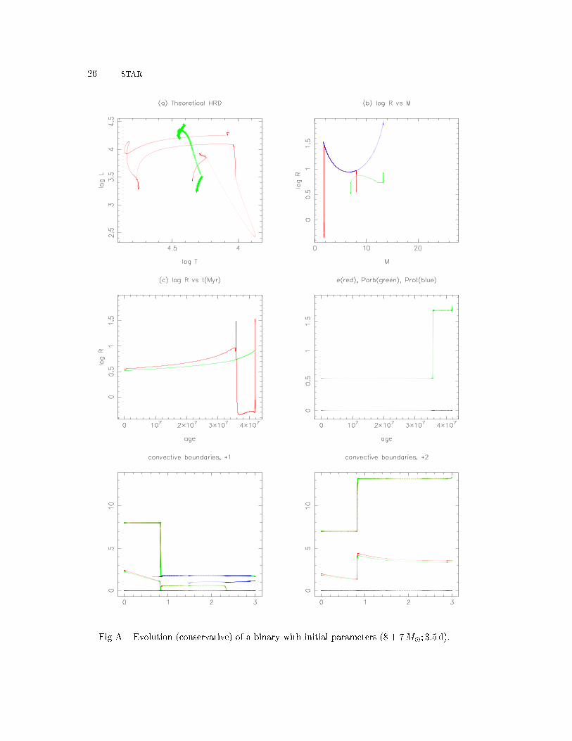
26 STAR

Fig A { Evolution ( onservative) of a binary with initial parameters (8 + 7M�; 3:5 d).

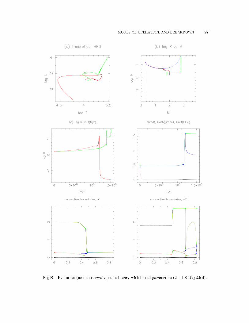
MODES OF OPERATION, AND BREAKDOWN 27

Fig B { Evolution (non- onservative) of a binary with initial parameters (2 + 1:8M�; 3:5 d).

28 STAR1.11 TEN TEST JOBSI have already mentioned that there are several di�erent kinds of job that one might wish todo with basi ally the same ode: onstru t a ZAMS, evolve a single star, evolve a binary, evolvea grid of single stars or of binaries, et . One philosophy is to have say 10 di�erent versions of the ode, to ope with 10 di�erent tasks; another is to put 10 di�erent options in the same ode. Ihave tried both philosophies at di�erent times, and I an only say I found the latter to be mu hthe simpler in the long term, though not in the short term.I am developing a suite of test jobs whi h is supposed to over most of the tasks that I have arried out at some time in the past. At present this omprises 10 tasks, whi h in a few wordsare:(i) Constru t a table of ZAMS models, at equal intervals of logM , possibly with di�erent metal-li ity than the `standard' solar Z: I sele ted � logM = 0:025, �1� logM � 2:3, somewhatarbitrarily. Higher masses are quite feasible, but I haven't often omputed them.(ii) Evolve a one-parameter grid of (e�e tively) single stars, with equally-spa ed logM sele tedexa tly from the ZAMS ompilation (i).(iii) Evolve non- onservatively a star with a mass somewhat di�erent from any in the Table in(i). It is a `pre-solar' star, starting on the ZAMS with slightly greater mass than the Sun,and with rapid rotation (3 d). Dynamo a tivity, mass loss and magneti braking bring it in� 4:6Gyr to solar mass and rotation rate.(iv) Evolve onservatively a (3-parameter) grid of 9 binaries where both masses ome from Table(i) { so that (log) mass-ratios are ne essarily 0.025, 0.05, ... ; 0.1 was used. Periods are alsoequally spa ed logarithmi ally. The �le also ontains the initial and output data for the runprodu ing Fig A.(v) As (iv), but only 4 of the 9 models, and non- onservative. The �le also ontains the initialand output data for the run produ ing Fig B.(vi) This is 7 sub-jobs. (a) Constru t a `Zero-Age Horizontal Bran h' model from a ZAMS model:evolve a 2:5M� star in whi h the omposition hange due to He burning is suppressed. (b)Constru t a ZAHB of stars with a given ore mass, starting from a late model of the previousrun and imposing a �xed mass-loss rate. An intermediate model has just under 2 M�, anda later model 0.76M�. These are the masses at the He ash of stars of initial mass 2 and1 M�, from run (ii). ( ) Regular evolution starting from model 25 of run (b). It gives thepost-He- ash evolution of an initial 2M� star. (d) Starting from model 117 of run (b), andas in run (a) allow the hydrogen to burn to helium but prevent the helium burning to arbon.The result is a 0:76M� star with a 0:47M� ore. (e) Regular evolution of the �nal model of(d), giving the post-He- ash evolution of a star of initial mass 1M�. (f) The same run as (b),but ontinuing until all the hydrogen envelope is gone so that the result is a 0:32M� ZAHeMSstar. (g) Starting from the end of (f), use arti� ial mass gain at a onstant (logarithmi ) rate,and with onstant timesteps, to onstru t a ZAHeMS from log M = -0.5 (0.05) 1.30. Run(vi) ontains a �le total.f9 whi h is the f9 �le of run (ii) augmented by the two post-He- ashruns ( ) and (e).(vii) Two runs that end with star 1 as a He WD and a CO WD respe tively, so you an havestarting models of su h stars for other purposes. (a) is a binary run, one of the 9 in (v), where�1 ends up as a He WD of 0:317M�; (b) starts from a ZAHeMS model of 0:531M�, and endswith a ooling sequen e of CO WD models.(viii) Constru t pre-main-sequen e, Hayashi-tra k, models with 0:5M� and in reasing luminosity.This is done by adding in an arti� ial energy-generation rate that is onstant throughout thestar and in reasing with time. Also follow the ontra tion of a pre-MS protostar. Startingfrom the last model of the previous run, let it ontra t thermally. Sin e deuterium is not

TEN TEST JOBS 29in luded, an important stage is missed out; but one ould no doubt add D to the 5 elementsnormally in luded.(ix) Use the TWINmodel to follow three binaries (BY Dra, RZ Eri, Z Her) where non- onservativepro esses in both stars are likely to be important.(x) Use the TWIN model to follow a very lose 4 + 2M� into RLOF, and then into onta t. Itdoesn't behave the way I think su h a onta t binary should behave, but it's my best shot sofar.The number of equations solved is the basi 11 in (i), (ii), (iv), (vi) and (vii), 17 in (iii), 18 in(v), 6 or 11 in (viii) and 33 in (ix), (x).All of these tasks an be done with the same omputational ` ore' ode, but with di�erent`shells' around it. In the ore we have to have some free parameters that multiply ertain bits ofphysi s: parameter zero means the bit of physi s (say, thermal energy generation, or RLOF, orstellar wind) is suppressed, and parameter unity means that it is in luded. We also have inputparameters that determine whi h kind of omputation the ore is to do. I'm afraid this hasturned out to be quite ompli ated for the TWIN mode. KTW = 1 means do the omponentssemi-independently, KTW = 2 means solve them simultaneously, often by doing (in e�e t) a loopDO II = 1, KTW. Although ea h shell separately might be supposed to be fairly simple, I haveopted for a single shell that tries to subsume all of the above tasks. If one ould be on�dent thatthe ore ode would never hange, it would make sense to have have 10 di�erent simple shells;but in pra ti e I have found that the ore is always developing, even if only in minor ways, andthat it is a lot of trouble to keep he king that a new version of the ore is ompatible with all10 shells: I �nd it slightly less trouble with a single more omplex shell.The set of �les that I will send on request, in luding the ode itself, an in lude 10 subdi-re tories alled run01, run02, ..., run10. Ea h subdire tory ontains the appropriate fort.22 andfort.23 (but renamed f22 and f23) to do an example from the list above. Some subdire tories ontain two or more sets. Some subdire tories also ontain the output �les that are obtained,typi ally fort.9 (abbreviated to f9). I wish I ould say that I did all ten runs with exa tly thesame ode (both ore and shell). In pra ti e I made a few modi� ations on the way, hoping thatI did this suÆ iently arefully that the new ode would still do the previous tasks in the samemanner.

30 STARSummaryA typi al Algol omprisesTwo stars of quite di�erent sizes.The one that is smallDoes nothing at all,But the other evolves to a risis.It expands, and ontinues to growTill it rea hes Ro he-lobe over ow.Then it transfers some massIn a thin stream of gasThat falls on the other below.The period starts to in rease,But the other star's not left in pea e.It starts to grow fast,Overtaking at last,And that's when the run has to ease.