Embed Size (px)
Citation preview
Developing a Soft Linkage between a detailed dynamic Input-Output macroeconomic model
and a MarkAl energy system model
François Briens [email protected]
and Nadia Maïzi nadia.maï[email protected]
Center for Applied Mathematics, Ecole des Mines Paristech (France)
19/11/2014

CONTENT
1. Current challenges to hybrid Energy-Economic modelling approaches
2. Our Input-Output Macroeconomic Model
3. Linking our Input-Output model to a MarkAl Model
4. Conclusion
2
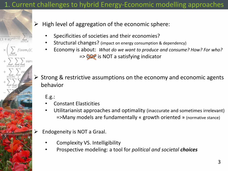
1. Current challenges to hybrid Energy-Economic modelling approaches
3
High level of aggregation of the economic sphere:
• Specificities of societies and their economies? • Structural changes? (impact on energy consumption & dependency)
• Economy is about: What do we want to produce and consume? How? For who?
=> GDP is NOT a satisfying indicator
Strong & restrictive assumptions on the economy and economic agents behavior
E.g.: • Constant Elasticities • Utilitarianist approaches and optimality (inaccurate and sometimes irrelevant)
=>Many models are fundamentally « growth oriented » (normative stance)
Endogeneity is NOT a Graal.
• Complexity VS. Intelligibility • Prospective modeling: a tool for political and societal choices
1. Current challenges to hybrid Energy-Economic modelling approaches
4
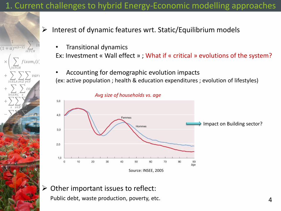
Interest of dynamic features wrt. Static/Equilibrium models
• Transitional dynamics Ex: Investment « Wall effect » ; What if « critical » evolutions of the system? • Accounting for demographic evolution impacts (ex: active population ; health & education expenditures ; evolution of lifestyles)
Other important issues to reflect: Public debt, waste production, poverty, etc.
Source: INSEE, 2005
Avg size of households vs. age
Impact on Building sector?
CONTENT
1. Current challenges to hybrid Energy-Economic modelling approaches
2. Our Input-Output Macroeconomic Model
3. Linking our Input-Output model to a MarkAl Model
4. Conclusion
5
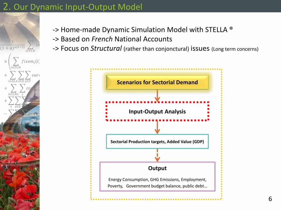
2. Our Dynamic Input-Output Model
6
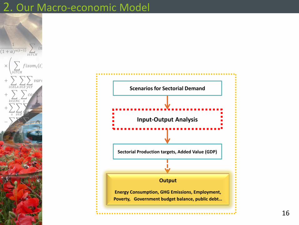
-> Home-made Dynamic Simulation Model with STELLA ® -> Based on French National Accounts -> Focus on Structural (rather than conjonctural) issues (Long term concerns)
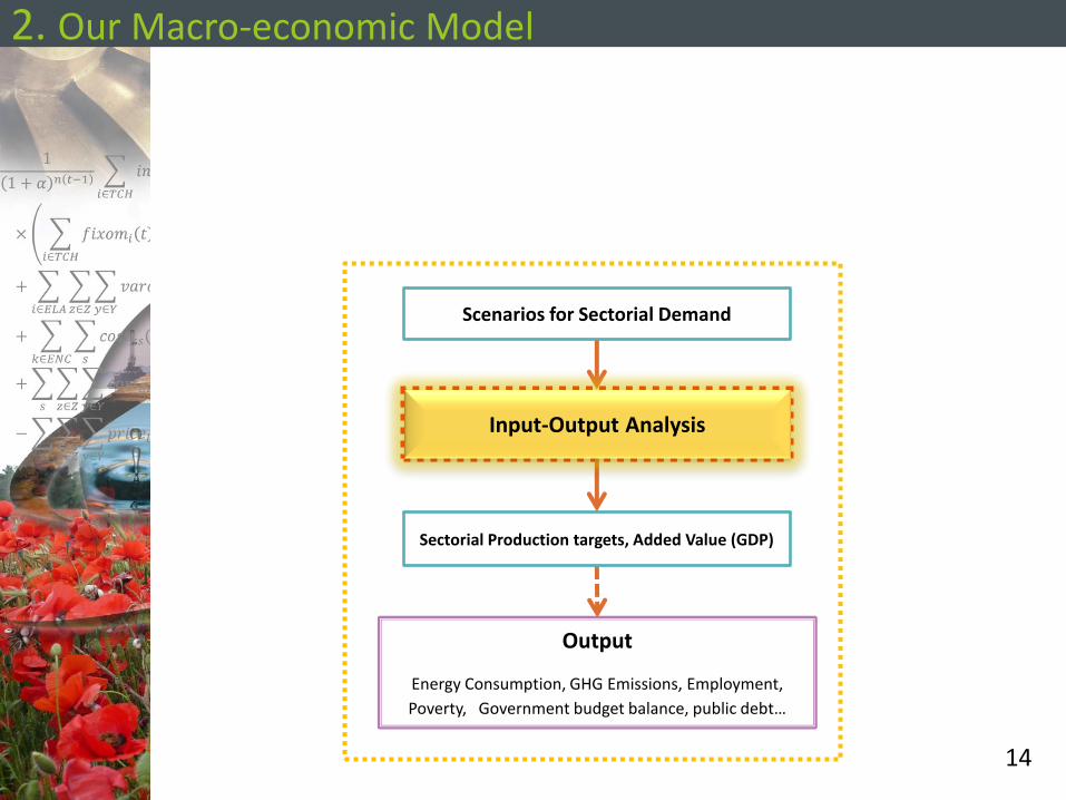
Sectorial Production targets, Added Value (GDP)
Input-Output Analysis
Output
Energy Consumption, GHG Emissions, Employment,
Poverty, Government budget balance, public debt…
Scenarios for Sectorial Demand Scenarios for Sectorial Demand
2. Our Macro-economic Model
7
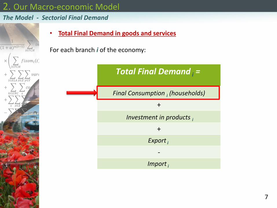
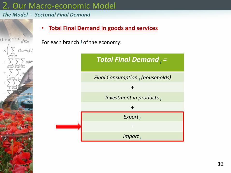
The Model - Sectorial Final Demand
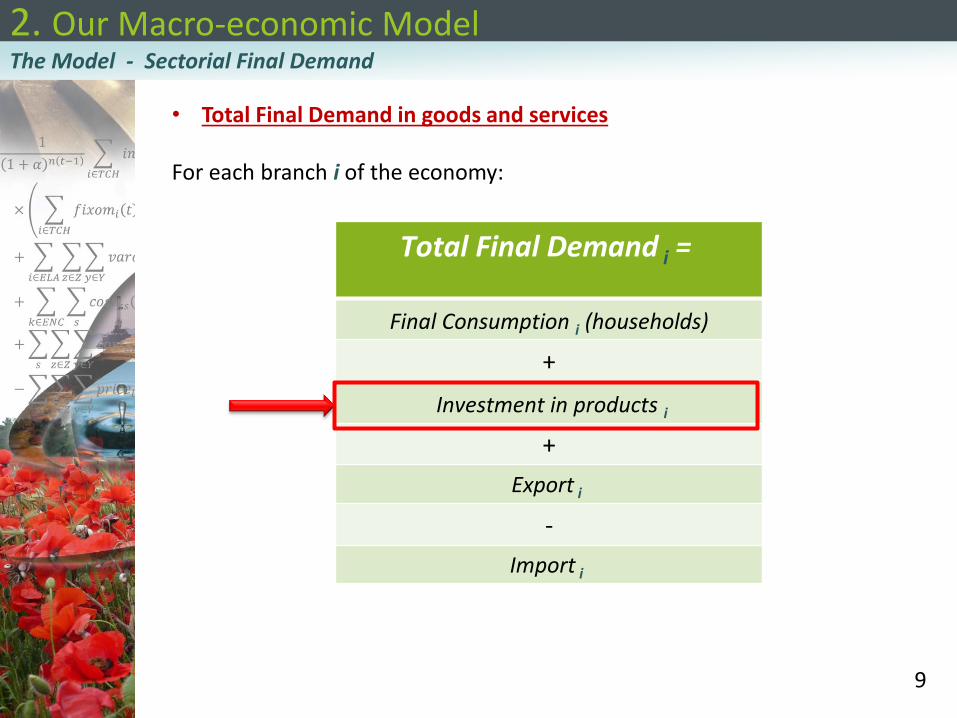
• Total Final Demand in goods and services
For each branch i of the economy:
Total Final Demand i =
Final Consumption i (households)
+
Investment in products i
+
Export i
-
Import i
2. Our Macro-economic Model
8
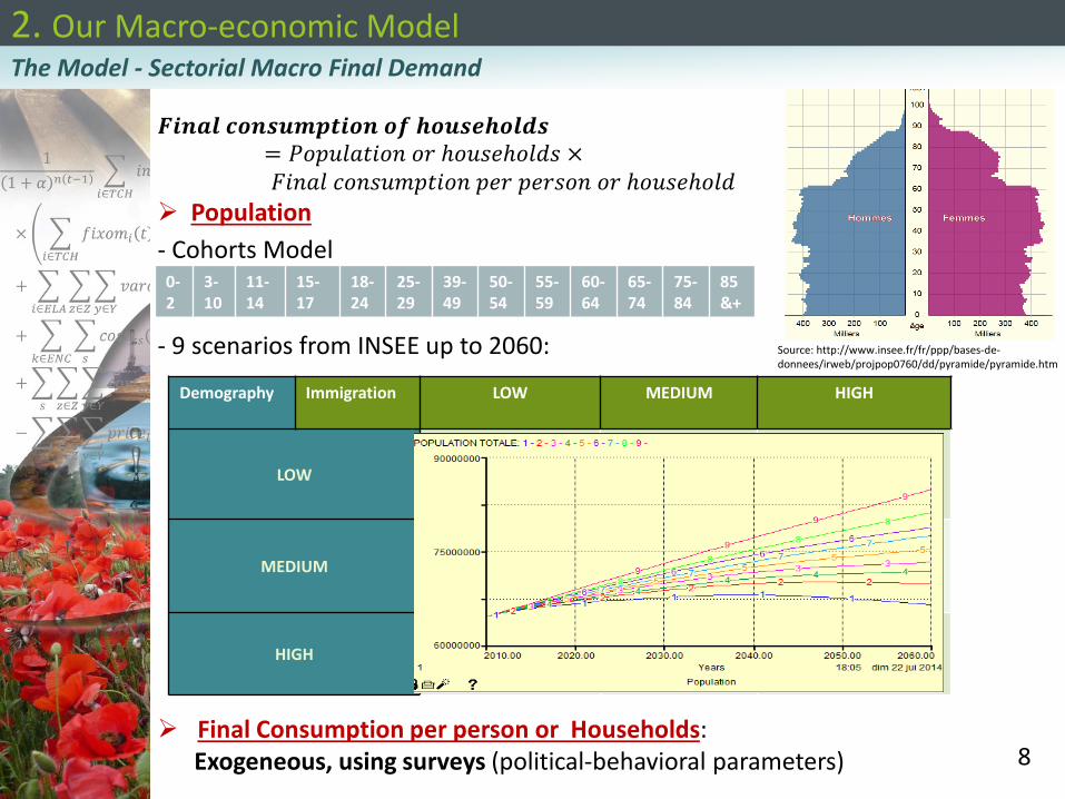
The Model - Sectorial Macro Final Demand
𝑭𝒊𝒏𝒂𝒍 𝒄𝒐𝒏𝒔𝒖𝒎𝒑𝒕𝒊𝒐𝒏 𝒐𝒇 𝒉𝒐𝒖𝒔𝒆𝒉𝒐𝒍𝒅𝒔= 𝑃𝑜𝑝𝑢𝑙𝑎𝑡𝑖𝑜𝑛 𝑜𝑟 ℎ𝑜𝑢𝑠𝑒ℎ𝑜𝑙𝑑𝑠 × 𝐹𝑖𝑛𝑎𝑙 𝑐𝑜𝑛𝑠𝑢𝑚𝑝𝑡𝑖𝑜𝑛 𝑝𝑒𝑟 𝑝𝑒𝑟𝑠𝑜𝑛 𝑜𝑟 ℎ𝑜𝑢𝑠𝑒ℎ𝑜𝑙𝑑
Population
- Cohorts Model - 9 scenarios from INSEE up to 2060:
Final Consumption per person or Households: Exogeneous, using surveys (political-behavioral parameters)
0-2
3-10
11-14
15-17
18-24
25-29
39-49
50-54
55-59
60-64
65-74
75-84
85 &+
Demography Immigration
LOW MEDIUM HIGH
LOW
MEDIUM
HIGH
Source: http://www.insee.fr/fr/ppp/bases-de-donnees/irweb/projpop0760/dd/pyramide/pyramide.htm
2. Our Macro-economic Model
9
The Model - Sectorial Final Demand
• Total Final Demand in goods and services
For each branch i of the economy:
Total Final Demand i =
Final Consumption i (households)
+
Investment in products i
+
Export i
-
Import i
2. Our Macro-economic Model
10
The Model - Sectorial Macro Final Demand
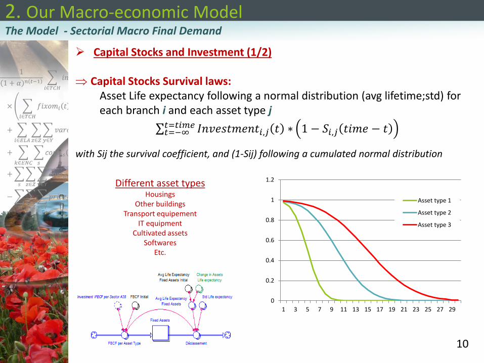
Capital Stocks and Investment (1/2) Capital Stocks Survival laws:
Asset Life expectancy following a normal distribution (avg lifetime;std) for each branch i and each asset type j
𝐼𝑛𝑣𝑒𝑠𝑡𝑚𝑒𝑛𝑡𝑖,𝑗 𝑡 ∗𝑡=𝑡𝑖𝑚𝑒𝑡=−∞ 1 − 𝑆𝑖,𝑗 𝑡𝑖𝑚𝑒 − 𝑡
with Sij the survival coefficient, and (1-Sij) following a cumulated normal distribution
Different asset types
Housings Other buildings
Transport equipement IT equipment
Cultivated assets Softwares
Etc.
0
0.2
0.4
0.6
0.8
1
1.2
1 3 5 7 9 11 13 15 17 19 21 23 25 27 29
Asset type 1
Asset type 2
Asset type 3
2. Our Macro-economic Model
11
The Model - Sectorial Macro Final Demand
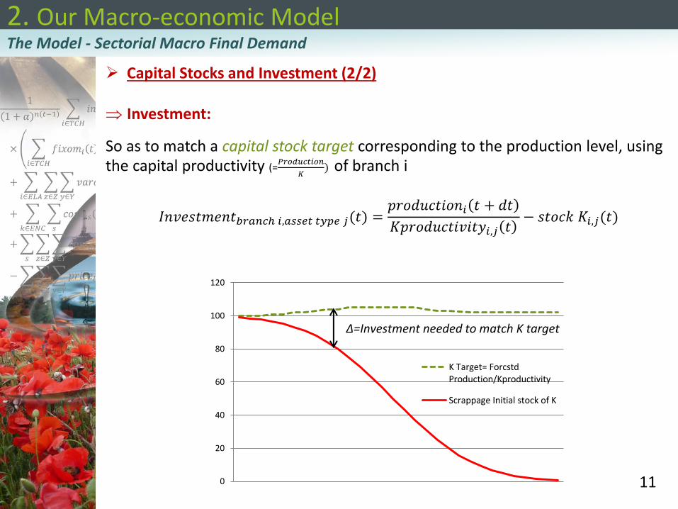
Capital Stocks and Investment (2/2) Investment:
So as to match a capital stock target corresponding to the production level, using the capital productivity (=𝑃𝑟𝑜𝑑𝑢𝑐𝑡𝑖𝑜𝑛
𝐾) of branch i
𝐼𝑛𝑣𝑒𝑠𝑡𝑚𝑒𝑛𝑡𝑏𝑟𝑎𝑛𝑐ℎ 𝑖,𝑎𝑠𝑠𝑒𝑡 𝑡𝑦𝑝𝑒 𝑗(𝑡) =𝑝𝑟𝑜𝑑𝑢𝑐𝑡𝑖𝑜𝑛𝑖 𝑡 + 𝑑𝑡
𝐾𝑝𝑟𝑜𝑑𝑢𝑐𝑡𝑖𝑣𝑖𝑡𝑦𝑖,𝑗 𝑡− 𝑠𝑡𝑜𝑐𝑘 𝐾𝑖,𝑗(𝑡)
0
20
40
60
80
100
120
K Target= ForcstdProduction/Kproductivity
Scrappage Initial stock of K
Δ=Investment needed to match K target
2. Our Macro-economic Model
12
The Model - Sectorial Final Demand
• Total Final Demand in goods and services
For each branch i of the economy:
Total Final Demand i =
Final Consumption i (households)
+
Investment in products i
+
Export i
-
Import i
2. Our Macro-economic Model
13
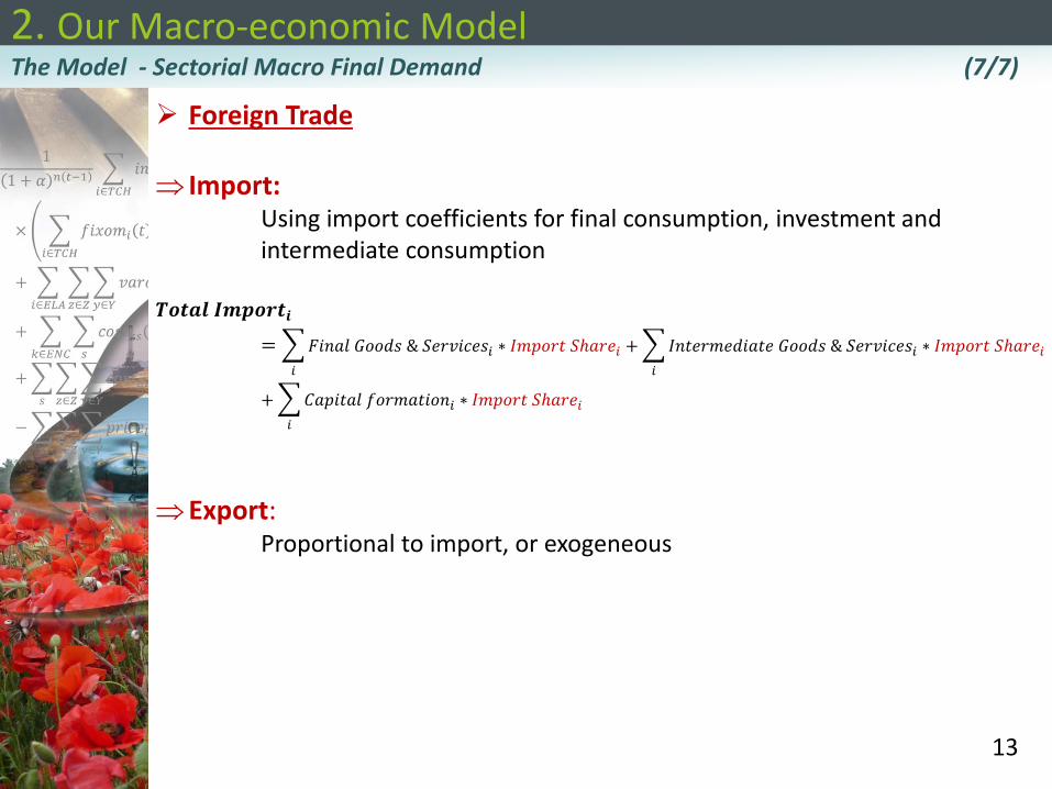
The Model - Sectorial Macro Final Demand (7/7)
Foreign Trade Import: Using import coefficients for final consumption, investment and intermediate consumption
𝑻𝒐𝒕𝒂𝒍 𝑰𝒎𝒑𝒐𝒓𝒕𝒊
= 𝐹𝑖𝑛𝑎𝑙 𝐺𝑜𝑜𝑑𝑠 & 𝑆𝑒𝑟𝑣𝑖𝑐𝑒𝑠𝑖𝑖
∗ 𝐼𝑚𝑝𝑜𝑟𝑡 𝑆ℎ𝑎𝑟𝑒𝑖 + 𝐼𝑛𝑡𝑒𝑟𝑚𝑒𝑑𝑖𝑎𝑡𝑒 𝐺𝑜𝑜𝑑𝑠 & 𝑆𝑒𝑟𝑣𝑖𝑐𝑒𝑠𝑖𝑖
∗ 𝐼𝑚𝑝𝑜𝑟𝑡 𝑆ℎ𝑎𝑟𝑒𝑖
+ 𝐶𝑎𝑝𝑖𝑡𝑎𝑙 𝑓𝑜𝑟𝑚𝑎𝑡𝑖𝑜𝑛𝑖𝑖
∗ 𝐼𝑚𝑝𝑜𝑟𝑡 𝑆ℎ𝑎𝑟𝑒𝑖
Export: Proportional to import, or exogeneous
2. Our Macro-economic Model
14
Sectorial Production targets, Added Value (GDP)
Input-Output Analysis
Output
Energy Consumption, GHG Emissions, Employment,
Poverty, Government budget balance, public debt…
Scenarios for Sectorial Demand
Input-Output Analysis
2. Our Macro-economic Model
15
The Model - Input-Output Analysis
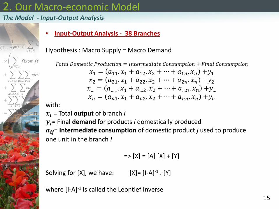
• Input-Output Analysis - 38 Branches
Hypothesis : Macro Supply = Macro Demand 𝑇𝑜𝑡𝑎𝑙 𝐷𝑜𝑚𝑒𝑠𝑡𝑖𝑐 𝑃𝑟𝑜𝑑𝑢𝑐𝑡𝑖𝑜𝑛 = 𝐼𝑛𝑡𝑒𝑟𝑚𝑒𝑑𝑖𝑎𝑡𝑒 𝐶𝑜𝑛𝑠𝑢𝑚𝑝𝑡𝑖𝑜𝑛 + 𝐹𝑖𝑛𝑎𝑙 𝐶𝑜𝑛𝑠𝑢𝑚𝑝𝑡𝑖𝑜𝑛
𝑥1 = 𝑎11. 𝑥1 + 𝑎12. 𝑥2 +⋯+ 𝑎1𝑛. 𝑥𝑛 +𝑦1 𝑥2 = 𝑎21. 𝑥1 + 𝑎22. 𝑥2 +⋯+ 𝑎2𝑛. 𝑥𝑛 +𝑦2 𝑥… = 𝑎…1. 𝑥1 + 𝑎…2. 𝑥2 +⋯+ 𝑎…𝑛. 𝑥𝑛 +𝑦… 𝑥𝑛 = 𝑎𝑛1. 𝑥1 + 𝑎𝑛2. 𝑥2 +⋯+ 𝑎𝑛𝑛. 𝑥𝑛 +𝑦𝑛
with: 𝒙𝒊 = Total output of branch i 𝒚𝒊= Final demand for products i domestically produced 𝒂𝒊𝒋= Intermediate consumption of domestic product j used to produce
one unit in the branch I
=> [X] = [A] [X] + [Y] Solving for [X], we have: [X]= [I-A]-1 . [Y] where [I-A]-1 is called the Leontief Inverse
2. Our Macro-economic Model
16
Sectorial Production targets, Added Value (GDP)
Input-Output Analysis
Output
Energy Consumption, GHG Emissions, Employment,
Poverty, Government budget balance, public debt…
Scenarios for Sectorial Demand
Output
Energy Consumption, GHG Emissions, Employment,
Poverty, Government budget balance, public debt…
2. Our Macro-economic Model
17
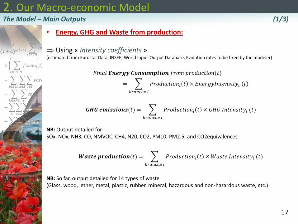
The Model – Main Outputs (1/3)
• Energy, GHG and Waste from production:
Using « Intensity coefficients » (estimated from Eurostat Data, INSEE, World Input-Output Database, Evolution rates to be fixed by the modeler)
𝐹𝑖𝑛𝑎𝑙 𝑬𝒏𝒆𝒓𝒈𝒚 𝑪𝒐𝒏𝒔𝒖𝒎𝒑𝒕𝒊𝒐𝒏 𝑓𝑟𝑜𝑚 𝑝𝑟𝑜𝑑𝑢𝑐𝑡𝑖𝑜𝑛(𝑡)
= 𝑃𝑟𝑜𝑑𝑢𝑐𝑡𝑖𝑜𝑛𝑖 𝑡 × 𝐸𝑛𝑒𝑟𝑔𝑦𝐼𝑛𝑡𝑒𝑛𝑠𝑖𝑡𝑦𝑖 (𝑡)
𝑏𝑟𝑎𝑛𝑐ℎ𝑒 𝑖
𝑮𝑯𝑮 𝒆𝒎𝒊𝒔𝒔𝒊𝒐𝒏𝒔(𝑡) = 𝑃𝑟𝑜𝑑𝑢𝑐𝑡𝑖𝑜𝑛𝑖 𝑡 × 𝐺𝐻𝐺 𝐼𝑛𝑡𝑒𝑛𝑠𝑖𝑡𝑦𝑖 (𝑡)
𝑏𝑟𝑎𝑛𝑐ℎ𝑒 𝑖
NB: Output detailed for: SOx, NOx, NH3, CO, NMVOC, CH4, N20, CO2, PM10, PM2.5, and CO2equivalences
𝑾𝒂𝒔𝒕𝒆 𝒑𝒓𝒐𝒅𝒖𝒄𝒕𝒊𝒐𝒏(𝑡) = 𝑃𝑟𝑜𝑑𝑢𝑐𝑡𝑖𝑜𝑛𝑖 𝑡 × 𝑊𝑎𝑠𝑡𝑒 𝐼𝑛𝑡𝑒𝑛𝑠𝑖𝑡𝑦𝑖 (𝑡)
𝑏𝑟𝑎𝑛𝑐ℎ𝑒 𝑖
NB: So far, output detailed for 14 types of waste (Glass, wood, lether, metal, plastic, rubber, mineral, hazardous and non-hazardous waste, etc.)
2. Our Macro-economic Model
18
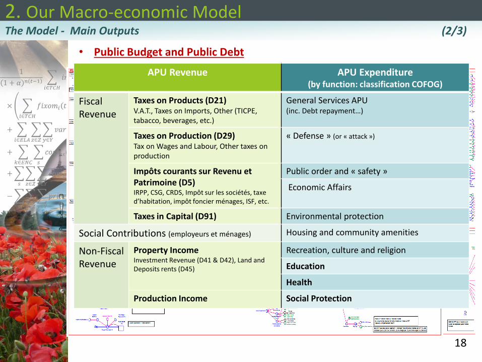
The Model - Main Outputs (2/3)
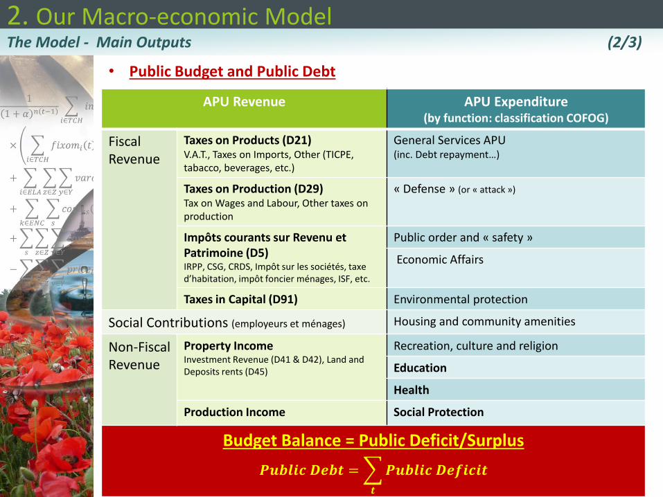
• Public Budget and Public Debt
APU Revenue APU Expenditure (by function: classification COFOG)
Fiscal Revenue
Taxes on Products (D21) V.A.T., Taxes on Imports, Other (TICPE, tabacco, beverages, etc.)
General Services APU (inc. Debt repayment…)
Taxes on Production (D29) Tax on Wages and Labour, Other taxes on production
« Defense » (or « attack »)
Impôts courants sur Revenu et Patrimoine (D5) IRPP, CSG, CRDS, Impôt sur les sociétés, taxe d’habitation, impôt foncier ménages, ISF, etc.
Public order and « safety »
Economic Affairs
Taxes in Capital (D91) Environmental protection
Social Contributions (employeurs et ménages) Housing and community amenities
Non-Fiscal Revenue
Property Income Investment Revenue (D41 & D42), Land and Deposits rents (D45)
Recreation, culture and religion
Education
Health
Production Income Social Protection
2. Our Macro-economic Model
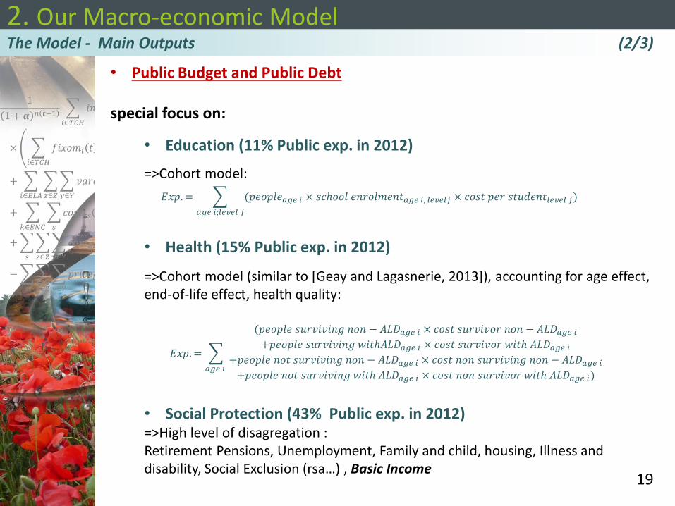
19
The Model - Main Outputs (2/3)
• Public Budget and Public Debt
special focus on:
• Education (11% Public exp. in 2012)
=>Cohort model:
𝐸𝑥𝑝. = (𝑝𝑒𝑜𝑝𝑙𝑒𝑎𝑔𝑒 𝑖 × 𝑠𝑐ℎ𝑜𝑜𝑙 𝑒𝑛𝑟𝑜𝑙𝑚𝑒𝑛𝑡𝑎𝑔𝑒 𝑖, 𝑙𝑒𝑣𝑒𝑙𝑗 × 𝑐𝑜𝑠𝑡 𝑝𝑒𝑟 𝑠𝑡𝑢𝑑𝑒𝑛𝑡𝑙𝑒𝑣𝑒𝑙 𝑗)
𝑎𝑔𝑒 𝑖;𝑙𝑒𝑣𝑒𝑙 𝑗
• Health (15% Public exp. in 2012)
=>Cohort model (similar to [Geay and Lagasnerie, 2013]), accounting for age effect, end-of-life effect, health quality:
𝐸𝑥𝑝. =
(𝑝𝑒𝑜𝑝𝑙𝑒 𝑠𝑢𝑟𝑣𝑖𝑣𝑖𝑛𝑔 𝑛𝑜𝑛 − 𝐴𝐿𝐷𝑎𝑔𝑒 𝑖 × 𝑐𝑜𝑠𝑡 𝑠𝑢𝑟𝑣𝑖𝑣𝑜𝑟 𝑛𝑜𝑛 − 𝐴𝐿𝐷𝑎𝑔𝑒 𝑖+𝑝𝑒𝑜𝑝𝑙𝑒 𝑠𝑢𝑟𝑣𝑖𝑣𝑖𝑛𝑔 𝑤𝑖𝑡ℎ𝐴𝐿𝐷𝑎𝑔𝑒 𝑖 × 𝑐𝑜𝑠𝑡 𝑠𝑢𝑟𝑣𝑖𝑣𝑜𝑟 𝑤𝑖𝑡ℎ 𝐴𝐿𝐷𝑎𝑔𝑒 𝑖
+𝑝𝑒𝑜𝑝𝑙𝑒 𝑛𝑜𝑡 𝑠𝑢𝑟𝑣𝑖𝑣𝑖𝑛𝑔 𝑛𝑜𝑛 − 𝐴𝐿𝐷𝑎𝑔𝑒 𝑖 × 𝑐𝑜𝑠𝑡 𝑛𝑜𝑛 𝑠𝑢𝑟𝑣𝑖𝑣𝑖𝑛𝑔 𝑛𝑜𝑛 − 𝐴𝐿𝐷𝑎𝑔𝑒 𝑖+𝑝𝑒𝑜𝑝𝑙𝑒 𝑛𝑜𝑡 𝑠𝑢𝑟𝑣𝑖𝑣𝑖𝑛𝑔 𝑤𝑖𝑡ℎ 𝐴𝐿𝐷𝑎𝑔𝑒 𝑖 × 𝑐𝑜𝑠𝑡 𝑛𝑜𝑛 𝑠𝑢𝑟𝑣𝑖𝑣𝑜𝑟 𝑤𝑖𝑡ℎ 𝐴𝐿𝐷𝑎𝑔𝑒 𝑖)
𝑎𝑔𝑒 𝑖
• Social Protection (43% Public exp. in 2012) =>High level of disagregation : Retirement Pensions, Unemployment, Family and child, housing, Illness and disability, Social Exclusion (rsa…) , Basic Income
2. Our Macro-economic Model
20
The Model - Main Outputs (2/3)
• Public Budget and Public Debt
APU Revenue APU Expenditure (by function: classification COFOG)
Fiscal Revenue
Taxes on Products (D21) V.A.T., Taxes on Imports, Other (TICPE, tabacco, beverages, etc.)
General Services APU (inc. Debt repayment…)
Taxes on Production (D29) Tax on Wages and Labour, Other taxes on production
« Defense » (or « attack »)
Impôts courants sur Revenu et Patrimoine (D5) IRPP, CSG, CRDS, Impôt sur les sociétés, taxe d’habitation, impôt foncier ménages, ISF, etc.
Public order and « safety »
Economic Affairs
Taxes in Capital (D91) Environmental protection
Social Contributions (employeurs et ménages) Housing and community amenities
Non-Fiscal Revenue
Property Income Investment Revenue (D41 & D42), Land and Deposits rents (D45)
Recreation, culture and religion
Education
Health
Production Income Social Protection
Budget Balance = Public Deficit/Surplus
𝑷𝒖𝒃𝒍𝒊𝒄 𝑫𝒆𝒃𝒕 = 𝑷𝒖𝒃𝒍𝒊𝒄 𝑫𝒆𝒇𝒊𝒄𝒊𝒕
𝒕
2. Our Macro-economic Model
21
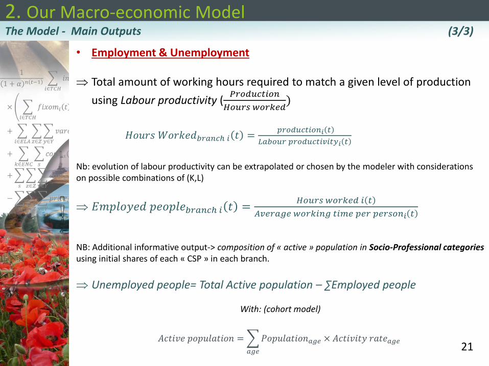
The Model - Main Outputs (3/3)
• Employment & Unemployment
Total amount of working hours required to match a given level of production
using Labour productivity (𝑃𝑟𝑜𝑑𝑢𝑐𝑡𝑖𝑜𝑛
𝐻𝑜𝑢𝑟𝑠 𝑤𝑜𝑟𝑘𝑒𝑑)
𝐻𝑜𝑢𝑟𝑠 𝑊𝑜𝑟𝑘𝑒𝑑𝑏𝑟𝑎𝑛𝑐ℎ 𝑖 𝑡 = 𝑝𝑟𝑜𝑑𝑢𝑐𝑡𝑖𝑜𝑛𝑖 𝑡
𝐿𝑎𝑏𝑜𝑢𝑟 𝑝𝑟𝑜𝑑𝑢𝑐𝑡𝑖𝑣𝑖𝑡𝑦𝑖 𝑡
Nb: evolution of labour productivity can be extrapolated or chosen by the modeler with considerations on possible combinations of (K,L)
𝐸𝑚𝑝𝑙𝑜𝑦𝑒𝑑 𝑝𝑒𝑜𝑝𝑙𝑒𝑏𝑟𝑎𝑛𝑐ℎ 𝑖 𝑡 =𝐻𝑜𝑢𝑟𝑠 𝑤𝑜𝑟𝑘𝑒𝑑 𝑖 𝑡
𝐴𝑣𝑒𝑟𝑎𝑔𝑒 𝑤𝑜𝑟𝑘𝑖𝑛𝑔 𝑡𝑖𝑚𝑒 𝑝𝑒𝑟 𝑝𝑒𝑟𝑠𝑜𝑛𝑖 𝑡
NB: Additional informative output-> composition of « active » population in Socio-Professional categories using initial shares of each « CSP » in each branch.
Unemployed people= Total Active population – ∑Employed people
With: (cohort model)
𝐴𝑐𝑡𝑖𝑣𝑒 𝑝𝑜𝑝𝑢𝑙𝑎𝑡𝑖𝑜𝑛 = 𝑃𝑜𝑝𝑢𝑙𝑎𝑡𝑖𝑜𝑛𝑎𝑔𝑒 × 𝐴𝑐𝑡𝑖𝑣𝑖𝑡𝑦 𝑟𝑎𝑡𝑒𝑎𝑔𝑒𝑎𝑔𝑒
2. Our Dynamic Input-Output Model
22
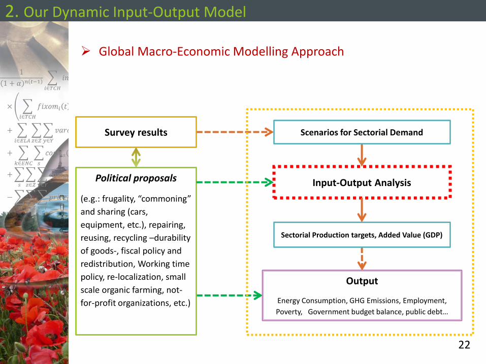
Global Macro-Economic Modelling Approach
Survey results
Sectorial Production targets, Added Value (GDP)
Input-Output Analysis
Output
Energy Consumption, GHG Emissions, Employment,
Poverty, Government budget balance, public debt…
Scenarios for Sectorial Demand
Political proposals
(e.g.: frugality, “commoning”
and sharing (cars,
equipment, etc.), repairing,
reusing, recycling –durability
of goods-, fiscal policy and
redistribution, Working time
policy, re-localization, small
scale organic farming, not-
for-profit organizations, etc.)

CONTENT
1. Current challenges to hybrid Energy-Economic modelling approaches
2. Our Input-Output Macroeconomic Model
3. Linking our Input-Output model to a MarkAl Model
4. Conclusion
23
3. Soft Linkage between dynamic Input-Output simulation model & MarkAl model
24
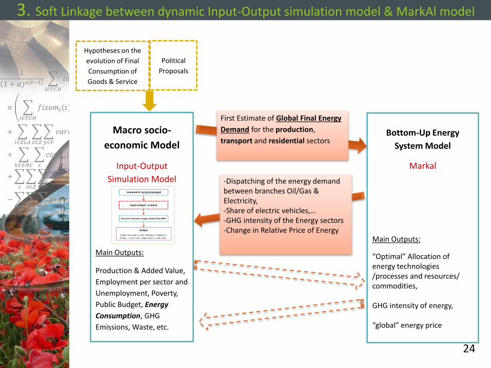
Macro socio-
economic Model
Input-Output
Simulation Model
Main Outputs:
Production & Added Value,
Employment per sector and
Unemployment, Poverty,
Public Budget, Energy
Consumption, GHG
Emissions, Waste, etc.
Hypotheses on the
evolution of Final
Consumption of
Goods & Service
Bottom-Up Energy
System Model
Markal
Main Outputs:
“Optimal” Allocation of energy technologies /processes and resources/ commodities, GHG intensity of energy, “global” energy price
First Estimate of Global Final Energy
Demand for the production,
transport and residential sectors
-Dispatching of the energy demand between branches Oil/Gas & Electricity, -Share of electric vehicles,… -GHG intensity of the Energy sectors -Change in Relative Price of Energy
Political
Proposals
CONTENT
1. Current challenges to hybrid Energy-Economic modelling approaches
2. Our Input-Output Macroeconomic Model
3. Linking our Input-Output model to a MarkAl Model
4. Conclusion
25
8. Conclusion (1/2)
26
Importance of dynamic features, disaggregation, flexibility of the economic sphere for the study of a diversity of contrasted scenarios of demand
About our macroeconomic model: a quite simple, accessible, powerful tool for common understanding and collective debate
Next steps: Surveys Scenario Building, Modeling, soft-linking and Analysis
Thank you for your attention
Q & A?
Éléments de bibliographie Assoumou, E. (2006). Modélisation MARKAL pour la planification énergétique long terme dans le ccontext français. PhD thesis, Ecole des Mines de Paris. Crassous, R. (2008). Modéliser le long terme dans un monde de 2nd rang: Application aux politiques climatiques. PhD thesis, Institut des Sciences et Industries du Vivant et de l’Environnement (Agro ParisTech). Duesenberry, J. S. (1949). Income, Saving and the Theory of Consumer Behavior. Cambrige (Mass.) Harvard University Press
Janssen, M. A. and Jager, W. (2001). Fashions, habits and changing preferences: Simulation of psychological factors affecting market dynamics. Journal of Economic Psychology, 22(6):745 – 772.
Latouche, S. (2009). Farewell to growth. Robert E. Lucas, J. (1976). Econometric policy evaluation: A critique. Carnegie-Rochester Conference Series on Public Policy, 1(1):19–46. O’Neill, D. W. (2012). Measuring progress in the degrowth transition to a steady state economy. Ecological Economics, 84(0):221 – 231. Victor, P. and Rosenbluth, G. (2007). Managing without growth. Ecological Economics, 61(2-3):492–504.
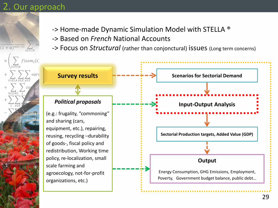
2. Our approach
29
-> Home-made Dynamic Simulation Model with STELLA ® -> Based on French National Accounts -> Focus on Structural (rather than conjonctural) issues (Long term concerns)
Survey results
Sectorial Production targets, Added Value (GDP)
Input-Output Analysis
Output
Energy Consumption, GHG Emissions, Employment,
Poverty, Government budget balance, public debt…
Scenarios for Sectorial Demand
Political proposals
(e.g.: frugality, “commoning”
and sharing (cars,
equipment, etc.), repairing,
reusing, recycling –durability
of goods-, fiscal policy and
redistribution, Working time
policy, re-localization, small
scale farming and
agroecology, not-for-profit
organizations, etc.)
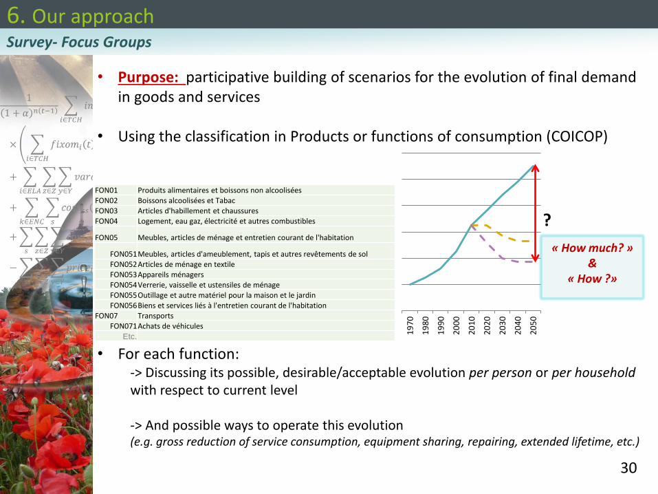
6. Our approach
30
Survey- Focus Groups
• Purpose: participative building of scenarios for the evolution of final demand in goods and services
• Using the classification in Products or functions of consumption (COICOP)
• For each function:
-> Discussing its possible, desirable/acceptable evolution per person or per household with respect to current level -> And possible ways to operate this evolution (e.g. gross reduction of service consumption, equipment sharing, repairing, extended lifetime, etc.)
FON01 Produits alimentaires et boissons non alcoolisées FON02 Boissons alcoolisées et Tabac
FON03 Articles d'habillement et chaussures FON04 Logement, eau gaz, électricité et autres combustibles
FON05 Meubles, articles de ménage et entretien courant de l'habitation
FON051 Meubles, articles d'ameublement, tapis et autres revêtements de sol FON052 Articles de ménage en textile
FON053 Appareils ménagers FON054 Verrerie, vaisselle et ustensiles de ménage
FON055 Outillage et autre matériel pour la maison et le jardin
FON056 Biens et services liés à l'entretien courant de l'habitation
FON07 Transports FON071 Achats de véhicules
Etc.
19
70
19
80
19
90
20
00
20
10
20
20
20
30
20
40
20
50
?
« How much? » &
« How ?»
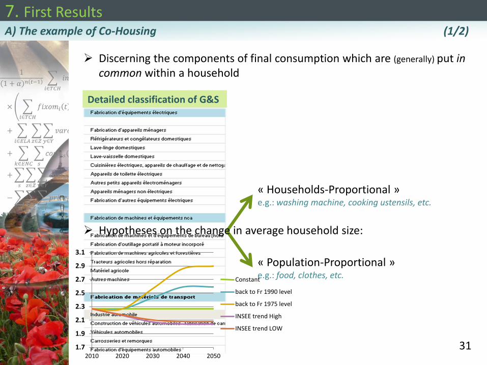
7. First Results
31
A) The example of Co-Housing (1/2)
Detailed classification of G&S
« Households-Proportional » e.g.: washing machine, cooking ustensils, etc.
« Population-Proportional » e.g.: food, clothes, etc.
Discerning the components of final consumption which are (generally) put in common within a household
Hypotheses on the change in average household size:
1.7
1.9
2.1
2.3
2.5
2.7
2.9
3.1
2010 2020 2030 2040 2050
Constant
back to Fr 1990 level
back to Fr 1975 level
INSEE trend High
INSEE trend LOW
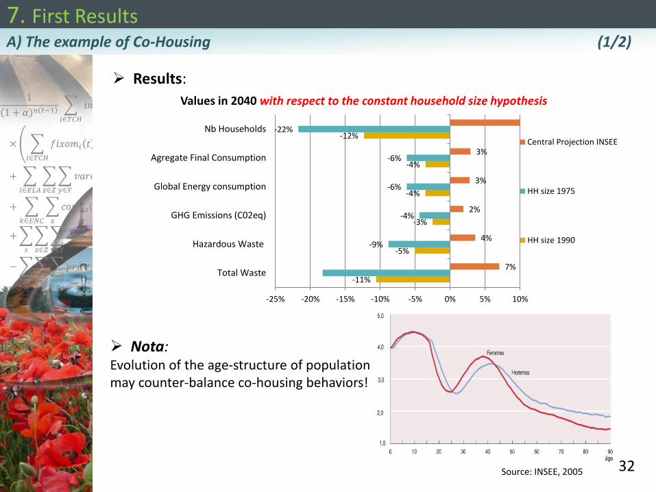
7. First Results
32
A) The example of Co-Housing (1/2)
Results:
Nota: Evolution of the age-structure of population may counter-balance co-housing behaviors!
Source: INSEE, 2005
-11%
-5%
-3%
-4%
-4%
-12%
-9%
-4%
-6%
-6%
-22%
7%
4%
2%
3%
3%
-25% -20% -15% -10% -5% 0% 5% 10%
Total Waste
Hazardous Waste
GHG Emissions (C02eq)
Global Energy consumption
Agregate Final Consumption
Nb Households
Values in 2040 with respect to the constant household size hypothesis
Central Projection INSEE
HH size 1975
HH size 1990
7. First Results
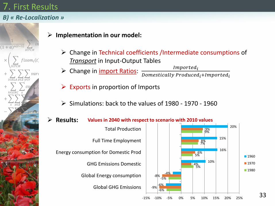
33
B) « Re-Localization »
Implementation in our model:
Change in Technical coefficients /Intermediate consumptions of
Transport in Input-Output Tables
Change in import Ratios: 𝐼𝑚𝑝𝑜𝑟𝑡𝑒𝑑𝑖
𝐷𝑜𝑚𝑒𝑠𝑡𝑖𝑐𝑎𝑙𝑙𝑦 𝑃𝑟𝑜𝑑𝑢𝑐𝑒𝑑𝑖+𝐼𝑚𝑝𝑜𝑟𝑡𝑒𝑑𝑖
Exports in proportion of Imports
Simulations: back to the values of 1980 - 1970 - 1960
Results:
-6%
-5%
5%
5%
7%
9%
-9%
-8%
4%
6%
8%
9%
-6%
-4%
10%
16%
15%
20%
-15% -10% -5% 0% 5% 10% 15% 20% 25%
Global GHG Emissions
Global Energy consumption
GHG Emissions Domestic
Energy consumption for Domestic Prod
Full Time Employment
Total Production
Values in 2040 with respect to scenario with 2010 values
1960
1970
1980


![Model-Based Decision Support in Energy Planningcore.ac.uk/download/pdf/33895947.pdf'The energy systems model MARKAL [24] is applied by IEA member countries for concerted analyses in](https://img.pdfslide.us/doc/110x75/5f8599ba8baab717cc5455ea/model-based-decision-support-in-energy-the-energy-systems-model-markal-24-is.jpg)