PALKANSAAJIEN TUTKIMUSLAITOS � TUTKIMUSSELOSTEITA

LABOUR INSTITUTE FOR ECONOMIC RESEARCH � DISCUSSION PAPERS

���

��-2%/(66�*52:7+

��,1�),1/$1'"

��(9,'(1&(�)520

��7+(�����V

���3HNND�6DXUDPR

$Q HDUOLHU YHUVLRQ RI WKLV SDSHU ZDV SUHVHQWHG DW WKH ��WK $QQXDO &RQIHUHQFH RI WKH (DVWHUQ (FRQRPLF$VVRFLDWLRQ� %RVWRQ 0$� 0DUFK ������ ����� , DP LQGHEWHG WR 0LND 0DOLUDQWD IRU XVHIXO FRPPHQWV� 7KLVSDSHU LV D SDUW RI WKH SURMHFW RQ MREV DQG JURZWK LQ )LQODQG LQ WKH ����V ILQDQFHG E\ WKH )LQQLVK 0LQLVWU\RI /DERXU DQG WKH (XURSHDQ 6RFLDO )XQG�

+HOVLQNL ����

,6%1 �������������

,661 ���������

3

Tiivistelmä

Tässä tutkimusselosteessa tarkastellaan talouskasvun ja työllisyyden välistä suhdetta Suomes-

sa 1990-luvulla. Lähtökohdaksi otetaan kaksi suomalaisessa keskustelussa esillä ollutta

tulkintaa. Toisen tulkinnan mukaan Suomessakin ollaan siirrytty uuteen aikakauteen, jota

luonnehtii aiempaa ripeämpi työn tuottavuuden kasvuvauhti ja jolloin kasvu ei enää työllistä niin

hyvin kuin joskus aikaisemmin (jobless growth -tulkinta). Tälle vastakkaisen toisen tulkinnan

mukaan kasvun ja työllisyyden välisessä suhteessa ei ole tapahtunut mitään muutosta. Työt-

tömyyden hidas lasku on kuvastanut ainoastaan kasvun laimeutta.

Tutkimusselosteessa esitetyn analyysin perusteella kumpikaan edellä esitetyistä tulkinnoista ei

kuvaa oikein kasvun ja työllisyyden välisen suhteen oleellisia piirteitä. Jobless growth -tulkinta

on virheellinen, koska työn tuottavuuden kasvuvauhti ei ole kiihtynyt 1990-luvulla pysyväisluon-

teisesti. Toisaalta näkemys, jonka mukaan kasvun ja työllisyyden välinen suhde on pysynyt

muuttumattomana, on myös harhaan johtava, koska erityisesti vuodet 1992%94 olivat poikkeuk-

sellisia. Tuolloin tuottavuuden kasvu oli poikkeuksellisen ripeätä, mikä johti tuottavuuden

kasvutrendin siirtymiseen ylöspäin. Myöhemmin kasvuvauhti on palautunut normaaliksi, mutta

trendin siirtymä on jäänyt pysyväksi.

Tutkimusselosteen aggregatiivinen analyysi perustuu yksinkertaisten rakenteellisten VAR-

mallien estimoimiseen. Estimointitulosten mukaan trendin siirtymän vuosina 1992%94 aiheutti-

vat positiiviset teknologishokit. Ehkä paras tulosten tulkintatapa on tulkita shokkien viime

kädessä kuvaavan vuosina 1992%94 toteutunutta voimakasta toimipaikkarakenteen muutosta

ja työvoiman siirtymistä keskimääräistä korkeamman tuotavuuden tason omaaviin toimipaikkoi-

hin. Tulkinta on sopusoinnussa olemassa olevien mikroaineistojen tarkasteluun perustuvien

analyysien kanssa.

4

Abstract

The purpose of the paper is to assess the validity of two interpretations which have been used

in the description of the relationship between employment growth and economic activity in

Finland during the 1990s. According to the New Era view the Finnish economy has moved into

a new era which, as a result of a faster-than-before rate of labour productivity growth, is

characterized by "jobless growth". According to the Cyclical Rebound view no change in the

rate of trend productivity growth has taken place. The productivity-led growth, which after the

very deep depression characterized the recovery of the economy, only reflected a normal

cyclical rebound.

The main result of my investigation is as follows. Neither the New Era view nor the Cyclical

Rebound view provides a telling interpretation about the developments of productivity and the

relationship between output and employment growth in the 1990s. Characterizing the years of

the recovery as reflecting a New Era which is associated with an increase in the rate of long-

run productivity growth is misleading, because that kind of change has not taken place. On the

other hand, the movements of productivity are hard to reconcile with the Cyclical Rebound view

because the years from 1992 to1994, especially, were exceptional. During the period

movements in productivity were not consistent with a pro-cyclical pattern, and, what is

important, the productivity trend shifted upwards. However, the shift was not associated with an

acceleration in the rate of trend productivity growth.

The upward shift was caused by a sequence of positive technology shocks, which were

identified by using a structural VAR model. The identifying restriction was rationalized by

utilizing a new Keynesian dynamic general equilibrium model. The positive technology shocks

which dominated the developments of aggregate productivity during the period from 1992 to

1994 mainly reflect micro-structural changes like business restructuring and labour reallocation

in manufacturing.

JEL Classification: E24, E32, J23, J24

Keywords: Jobless growth, technology shocks, business cycles

5

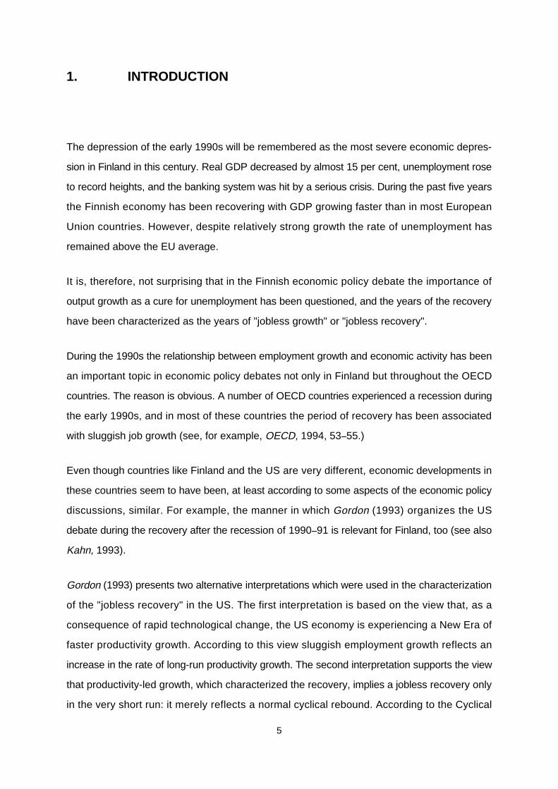
1. INTRODUCTION

The depression of the early 1990s will be remembered as the most severe economic depres-

sion in Finland in this century. Real GDP decreased by almost 15 per cent, unemployment rose

to record heights, and the banking system was hit by a serious crisis. During the past five years

the Finnish economy has been recovering with GDP growing faster than in most European

Union countries. However, despite relatively strong growth the rate of unemployment has

remained above the EU average.

It is, therefore, not surprising that in the Finnish economic policy debate the importance of

output growth as a cure for unemployment has been questioned, and the years of the recovery

have been characterized as the years of "jobless growth" or "jobless recovery".

During the 1990s the relationship between employment growth and economic activity has been

an important topic in economic policy debates not only in Finland but throughout the OECD

countries. The reason is obvious. A number of OECD countries experienced a recession during

the early 1990s, and in most of these countries the period of recovery has been associated

with sluggish job growth (see, for example, OECD, 1994, 53%55.)

Even though countries like Finland and the US are very different, economic developments in

these countries seem to have been, at least according to some aspects of the economic policy

discussions, similar. For example, the manner in which Gordon (1993) organizes the US

debate during the recovery after the recession of 1990%91 is relevant for Finland, too (see also

Kahn, 1993).

Gordon (1993) presents two alternative interpretations which were used in the characterization

of the "jobless recovery" in the US. The first interpretation is based on the view that, as a

consequence of rapid technological change, the US economy is experiencing a New Era of

faster productivity growth. According to this view sluggish employment growth reflects an

increase in the rate of long-run productivity growth. The second interpretation supports the view

that productivity-led growth, which characterized the recovery, implies a jobless recovery only

in the very short run: it merely reflects a normal cyclical rebound. According to the Cyclical

6

Rebound view no change in the rate of trend productivity growth has taken place. This also

means that the relationship between output growth and employment growth has remained

unchanged.

Both of these views have had their advocates in Finland, too. The purpose of this paper is to

analyse which one, if any, provides the best description of the connection between output

growth and employment growth in Finland during the 1990s. I will analyse not only the phase

of the recovery but also the years of the depression. Therefore I shall also analyse the period

when the rates of output and employment growth have been negative.

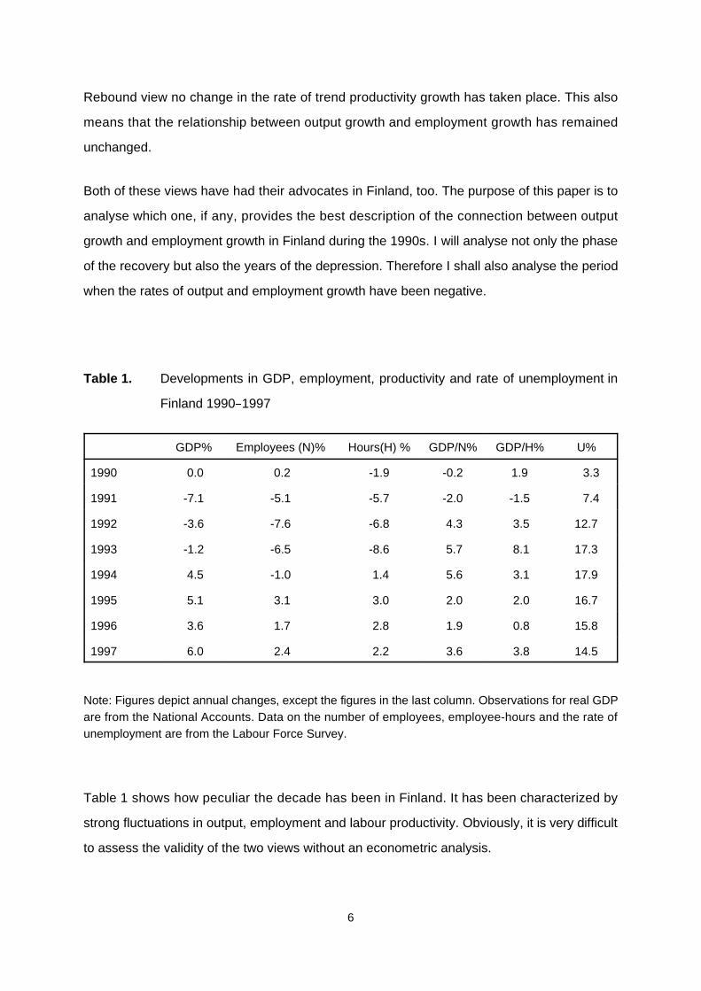
Table 1. Developments in GDP, employment, productivity and rate of unemployment in

Finland 1990%1997

GDP% Employees (N)% Hours(H) % GDP/N% GDP/H% U%

1990 0.0 0.2 -1.9 -0.2 1.9 3.3

1991 -7.1 -5.1 -5.7 -2.0 -1.5 7.4

1992 -3.6 -7.6 -6.8 4.3 3.5 12.7

1993 -1.2 -6.5 -8.6 5.7 8.1 17.3

1994 4.5 -1.0 1.4 5.6 3.1 17.9

1995 5.1 3.1 3.0 2.0 2.0 16.7

1996 3.6 1.7 2.8 1.9 0.8 15.8

1997 6.0 2.4 2.2 3.6 3.8 14.5

Note: Figures depict annual changes, except the figures in the last column. Observations for real GDPare from the National Accounts. Data on the number of employees, employee-hours and the rate ofunemployment are from the Labour Force Survey.

Table 1 shows how peculiar the decade has been in Finland. It has been characterized by

strong fluctuations in output, employment and labour productivity. Obviously, it is very difficult

to assess the validity of the two views without an econometric analysis.

7

In this paper I analyse developments in output, employment and productivity by estimating

simple structural VAR models. This is, of course, only one alternative. The basic difficulty in

assessing the relevance of the two interpretations is to unscramble the productivity trend from

cyclical movements. Gordon (1993), and many others, have conducted their investigations by

assuming that productivity trend can be modelled as a deterministic trend which, however, may

have breaks. The approach utilized in this paper allows the productivity trend to be stochastic.

When structural VAR models are used in modelling developments in output, employment and

productivity, the identification of the relevant shocks which drive the movements in these

variables becomes the crucial issue. In assessing the validity of the two interpretations the role

of technology or in the VAR context the role of technology shocks becomes important.

It is, however, not clear how a technology shock is defined. In this paper, technology shocks

are identified by assuming that unlike other shocks they have a permanent effect on the level

of labour productivity A broad class of theoretical models satisfies this restriction. This paper

draws mainly on Gali (1999), in which the main identifying restriction is rationalized by a new

Keynesian dynamic general equilibrium model.

Since I will only use data on GDP and aggregate labour input, the examination will be highly

aggregative. This is consistent with the utilization of representative agent models as a macro-

theoretical basis. It may, however, make the interpretation of results difficult. By employing only

aggregative data it is difficult, for example, to say anything about the role of industrial

restructuring as a determinant of aggregate labour productivity. In order to examine the impor-

tance of industrial restructuring the use of micro data is necessary. When interpreting the

results, I utilize some recent Finnish studies which are based on the use of micro data (see

Maliranta, 1997).

The main result of my investigation is as follows. Neither the New Era nor the Cyclical Rebound

view provides a telling interpretation about the developments of productivity and the relation-

ship between output and employment growth in the 1990s.

Characterizing the years of the recovery as reflecting a new era which is associated with an

increase in the rate of long-run productivity growth is misleading, because that kind of change

8

has not taken place. On the other hand, the movements of productivity are hard to reconcile

with the Cyclical Rebound view because the years from 1992 to1994, especially, were

exceptional. During that period movements in productivity were not consistent with a pro-

cyclical pattern.

I argue that those years comprise a special period during which productivity growth was

exceptionally high (see Table 1). Productivity growth evened out later, but as a result of the

period of strong growth the productivity trend shifted upwards. It is the shift that makes the

period unusual.

According to the New Era view the slope of the trend should have changed, whereas according

to the Cyclical Rebound view no change in the trend should have taken place. Both

interpretations give an incomplete description about the developments of productivity.

Within the aggregative framework the source of the shift was positive technology shocks. It will,

however, be seen that, when results from more disaggregative examinations are used in

interpreting the results, the positive technology shocks cannot easily be interpreted as

technological improvements at plant level. They may rather reflect the consequences of

business restructuring.

In OECD’s Jobs study (OECD, 1994, 55) the experiences from different countries are

summarized as follows: "On balance, while the recovery in employment has been slower in

some countries than in the past, this would appear to reflect an initially weaker rebound in

output rather than "jobless growth" as such. " As far as Finland is concerned, the results of this

paper do not support this kind of interpretation. In Finland productivity growth was "excessive"

both during the depression years from 1992 to 1993, when GDP decreased, and in 1994,

which was the first year of recovery (see Table 1). Because the period of "excessive" growth

lasted for only three years, speaking of a New Era of "jobless growth" is, however, misleading.

9

2. THE FRAMEWORK AND THE DATA

The econometric analysis will be based on the estimation of simple structural VAR models,

which, however, enables one to model dynamic interdependences between real output,

employment and labour productivity. Because the main source of fluctuations are (exogenous)

shocks which operate through a propagation mechanism, the identification of relevant shocks

becomes the crucial task.

The two views, the New Era and the Cyclical Rebound view, differ at least in one respect: the

first interpretation emphasizes the role of technological change as a factor which has altered

the relationship between employment and output growth, i.e. it has accelerated long-run

productivity growth. According to the second interpretation nothing like this has happened.

If one wants to explore these interpretations by utilizing structural VAR models, the identifi-

cation of technology shocks is therefore necessary. Of course, there does not exist a unique

way of estimating these shocks. One can, however, rationalize some specific identifying

restrictions by utilizing theoretical models which provide the relevant restrictions.

In this paper, the identification of technology shocks is based on the following identifying

assumption: only technology shocks have a permanent effect on the level of labour produc-

tivity. This also means that only technological shocks can cause permanent shifts in trend

productivity.

A wide class of theoretical models fulfills this restriction. It includes both real business cycle

(RBC) models and new Keynesian models. This paper rests mainly on Gali (1999), which

utilizes a new Keynesian dynamic general equilibrium model. It also discusses the relevant

literature. Essentially the same identifying assumption has also been used, for example, by

Dolado and Jimeno (1997). (See also Castillo, Dolado and Jimeno, 1998; Jacobson, Vredin

and Warne, 1997, 1998.)

Obviously, not every theoretical model, whether it belongs to the class of RBC, new Keynesian

or other models, is useful when, for example, the issue of "jobless growth" is discussed. The

10

model should have the property that positive technology shocks decrease the level of

employment at least in the short run. Gali’s (1999) model has this property. It is a simple

representative agent model with monopolistic competition, sticky prices and variable effort. The

basic feature of the model is best seen in the special case when the money supply is assumed

to be exogenous. In that case a constant money supply and predetermined prices imply that

real balances and, consequently, aggregate demand, and output remain unchanged during the

period when the technology shock occurs. If the technology shock is positive, the same output

can be produced by less input.

This kind of response is not consistent with predictions of the conventional RBC models. In

those models positive technology shocks, by shifting demand for labour schedules, have an

immediate positive effect on the level of employment.

Gali’s (1999) model is one alternative among various models which can be used when the

central identifying restriction is rationalized (for a discussion, see also Basu, Fernald and

Kimball, 1998). It is attractive because it enables one to identify technology shocks by using a

very simple two-variable VAR model. Simplicity is, of course, achieved by some strong

assumptions.

When a two-variable model is used, one can identify two types of shocks. The way technology

shocks are identified means that the other type of shocks, non-technology shocks, can have

only a transitory effect on the level of productivity. Non-technology shocks, which can be

aggregate demand shocks, can, however, have a permanent effect on the level of real output.

In their pioneering work Blanchard and Quah (1989) separated aggregate supply shocks from

aggregate demand shocks by assuming, in the spirit of the vertical long-run Phillips curve

paradigm, that only aggregate supply shocks can have a permanent influence on real output.

The assumption is stronger than the one used in this paper. (In Sauramo, 1998a, I examined

the causes of the Finnish depression by employing the vertical long-run Phillips curve

paradigm. The paper illustrates that, by utilizing Finnish data, it is difficult to identify reasonable

aggregate supply and aggregate demand shocks which would be consistent with that

paradigm.)

11

The identification of technology shocks can be based on the estimation of bivariate models

which utilize data on real output and labour input. For example, Gali (1999) estimates models

with labour productivity and labour input being the two variables. I will estimate bivariate

models which describe joint dependence between productivity and real output. By definition,

the models also describe joint dependence between productivity and labour input.

The use of data on labour productivity is perhaps the simplest way of identifying technology

shocks when VAR models are used. A relevant alternative is to utilize data on total factor

productivity, if that kind of data is available. For instance, Gali and Hammour (1991), Malley

and Muscatelli (1997) and Malley, Muscatelli and Woitek (1998) employ such data. The

identifying restrictions they utilized also differed from the long-run restriction to be used in this

paper.

The empirical exploration is based on the utilization of aggregative quarterly data. For real

output I use data on real GDP. For labour input I use quarterly data on the number of

employees. A relevant alternative would have been to use data on total hours worked by

employees. I have used it earlier (see Sauramo, 1998b). One reason for my choice is that the

use of the number of employees enables one to relate the investigation to the number of jobs,

and, correspondingly, to "jobless growth". Also, the quality of the quarterly data on the number

of employees is (according to my experience) most probably better than that of hours.

In the construction of quarterly data on productivity, the basic problem is that, unlike Annual

National Accounts, Quarterly National Accounts do not include data on labour input. Quarterly

series for labour input must be constructed by utilizing the Labour Force Survey.

The quarterly data, which is seasonally adjusted, covers the period 1975:1%1998:2. Even

though the period is relatively short, the series are not unbroken. (They contain a couple of

breaks.) For the years of depression and recovery the series , however, do not contain breaks.

The main results of the paper should therefore not be affected by them.

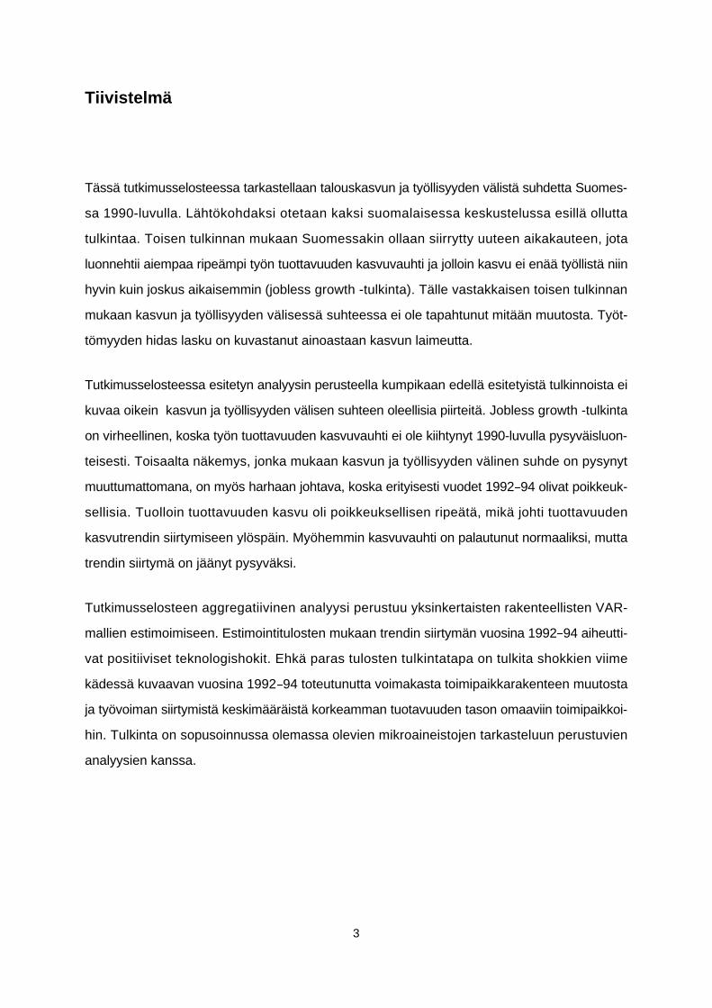
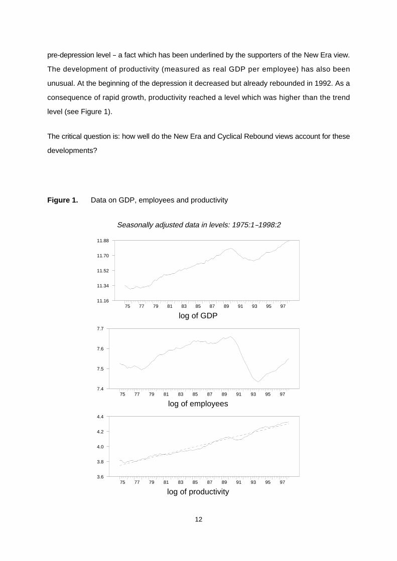
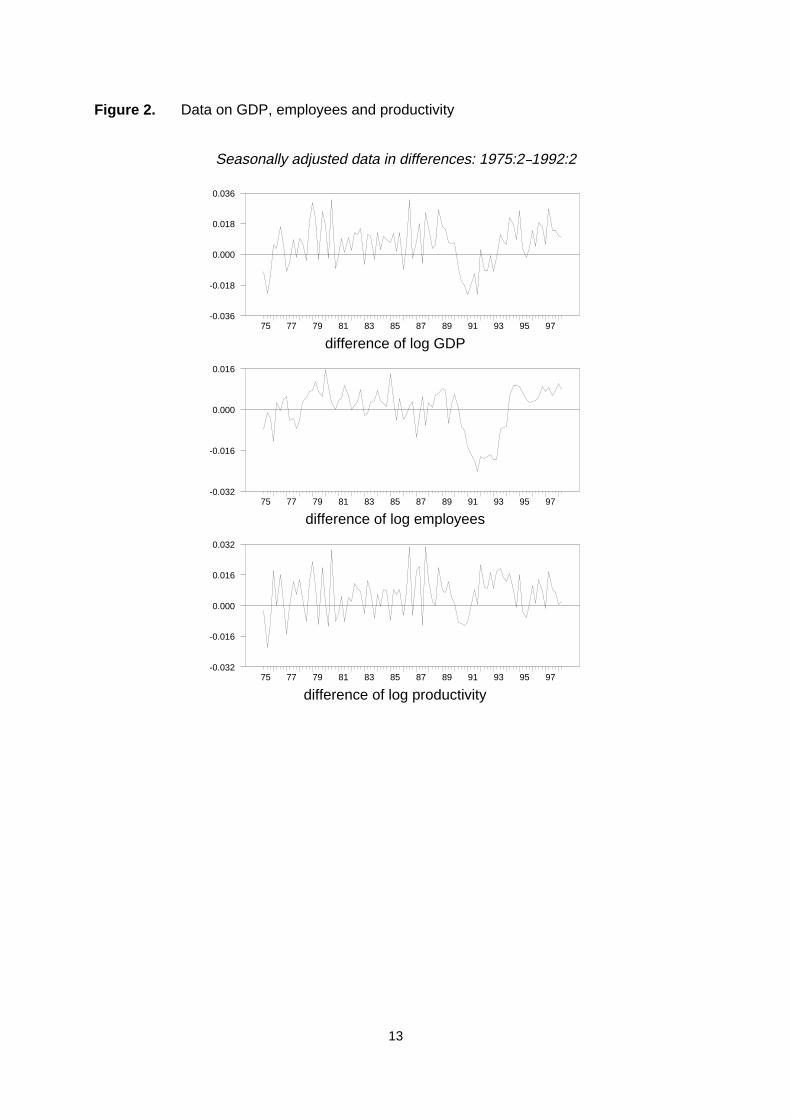
Figures 1 and 2 depict the data both in logs and log differences. The exceptionality of the early

1990s is seen in every panel of Figure 1. After the collapse of real GDP in 1991, it took five

years before the pre-depression level was reached. The number of employees is still below its

12

log of GDP75 77 79 81 83 85 87 89 91 93 95 97

11.16

11.34

11.52

11.70

11.88

log of employees75 77 79 81 83 85 87 89 91 93 95 97

7.4

7.5

7.6

7.7

log of productivity75 77 79 81 83 85 87 89 91 93 95 97

3.6

3.8

4.0

4.2

4.4

pre-depression level % a fact which has been underlined by the supporters of the New Era view.

The development of productivity (measured as real GDP per employee) has also been

unusual. At the beginning of the depression it decreased but already rebounded in 1992. As a

consequence of rapid growth, productivity reached a level which was higher than the trend

level (see Figure 1).

The critical question is: how well do the New Era and Cyclical Rebound views account for these

developments?

Figure 1. Data on GDP, employees and productivity

Seasonally adjusted data in levels: 1975:1%1998:2

13

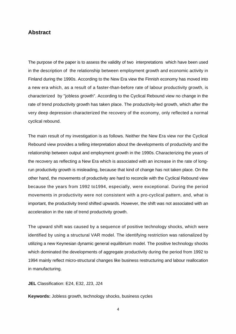
difference of log GDP75 77 79 81 83 85 87 89 91 93 95 97

-0.036

-0.018

0.000

0.018

0.036

difference of log employees75 77 79 81 83 85 87 89 91 93 95 97

-0.032

-0.016

0.000

0.016

difference of log productivity75 77 79 81 83 85 87 89 91 93 95 97

-0.032

-0.016

0.000

0.016

0.032

Figure 2. Data on GDP, employees and productivity

Seasonally adjusted data in differences: 1975:2%1992:2

14

3. NEW ERA VERSUS CYCLICAL REBOUND

The answer is based on the results from the estimation of a two-variable productivity-output

model. According to the standard Augmented Dickey-Fuller tests (log of) output (y) and (log of)

labour productivity (y-n) are integrated of order one. To achieve stationarity, first-differencing

is therefore necessary (see Figure 2).

The estimation of the unconstrained reduced form is based on the assumption that

xt = (�yt -�nt , �yt) is a covariance stationary process. The model is therefore estimated in the

first-difference form. Three lags are used, with Schwarz and Hannan-Quinn information criteria

being the main decision-making criteria. The estimation period is 1976:1%1998:2.

The identification of the two shocks takes place in a similar fashion to that in numerous studies

which utilize long-run identifying restrictions. In the two-variable case three constraints are

needed for just-identification.The two types of shocks, technology shocks and non-technology

shocks, are separated by the long-run restriction: only technology shocks have a permanent

influence on the level of productivity. Two additional constraints are given by the assumption

that shocks are mutually orthogonal and that their variances equal unity.

The manner in which technology shocks are defined implies that only technology shocks can

cause shifts in the (stochastic) productivity trend. (Since the equations of the unconstrained

reduced form contain constants, the productivity trend has a deterministic drift component.)

Even though the other shock, the non-technology shock, affects the level of productivity only

temporarily, it can have a permanent effect on the level of real output. In Gali’s (1999)

theoretical model the other shock was a monetary shock, i.e. an aggregate demand shock.

Within the empirical two-variable framework of this paper it is impossible to say in advance

whether the other shock is best regarded as an aggregate demand or aggregate supply shock.

The nature of the shocks will be illustrated by using impulse responses and forecast-error

variance decompositions. I also utilize evidence from a three-variable productivity-output-prices

-model by which one can examine how the relevant shocks affect prices.

1

1 I owe special thanks to Jordi Gali for kindly providing the RATS code for performing thecomputations.

15

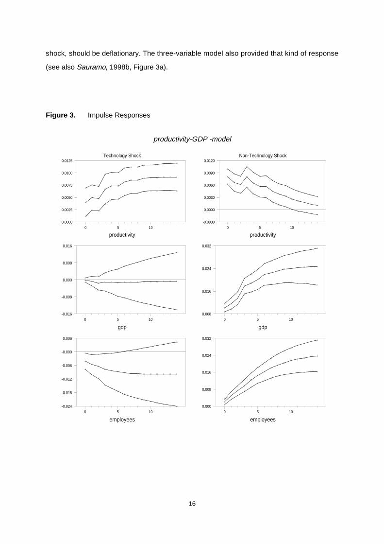
Figure 3 displays the impulse responses associated with the two shocks together with one-

standard error confidence bands.1 Variables are expressed in levels even though the model

was estimated in the difference form. The impulse responses for the number of employees are

easy to derive after computing impulse responses for productivity and output. Confidence

bands for impulse responses were computed by utilizing a Monte Carlo method which is based

on sampling from the estimated asymptotic distribution of the VAR coefficients and the

covariance matrix of the innovations. In each draw the sample size amounted to 500.

In the figure the left-hand panel depicts the responses to the shock which is supposed to be a

positive technology shock. They are consistent with that kind of interpretation. The positive

technology shock increases the level of productivity both in the short and longer run. Its effect

on the level of output is ambiguous, but it decreases employment at least in the short run. The

responses are in accordance with various sticky price models. Within the class of those

models, the short-run response of output to a positive technology shock may even be

contractionary (see Basu, Fernald and Kimball, 1998).

The right-hand panel of Figure 3 depicts impulse responses which are associated with the non-

technology shock. A positive non-technology shock is expansionary. It increases output and

employment both in the short and long run. It also has a positive effect on the level of

productivity in the short run. By definition, the shock does not affect the level of productivity in

the long run. The responses are consistent with the interpretation that the non-technology

shock is an aggregate demand shock.

The interpretation is confirmed by the results from the estimation of a three-variable

productivity-output-prices model. (In the model, the Consumer Price Index was used as the

price variable. The estimation results are available upon request. For an analogous estimation

see Sauramo, 1998b, in which employee hours were used as the labour input variable.)

According to the results, the positive non-technology shock is inflationary % a feature which a

positive aggregate demand shock should have within the standard aggregate demand

aggregate supply framework. On the other hand, a positive technology shock, i.e. a supply

16

Technology Shock

productivity0 5 10

0.0000

0.0025

0.0050

0.0075

0.0100

0.0125

gdp0 5 10

-0.016

-0.008

0.000

0.008

0.016

employees0 5 10

-0.024

-0.018

-0.012

-0.006

-0.000

0.006

Non-Technology Shock

productivity0 5 10

-0.0030

0.0000

0.0030

0.0060

0.0090

0.0120

gdp0 5 10

0.008

0.016

0.024

0.032

employees0 5 10

0.000

0.008

0.016

0.024

0.032

shock, should be deflationary. The three-variable model also provided that kind of response

(see also Sauramo, 1998b, Figure 3a).

Figure 3. Impulse Responses

productivity-GDP -model

17

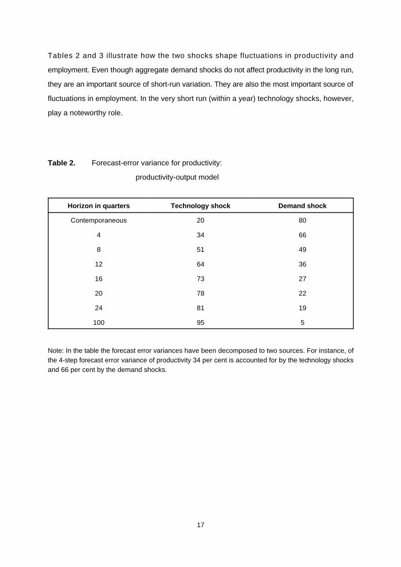
Tables 2 and 3 illustrate how the two shocks shape fluctuations in productivity and

employment. Even though aggregate demand shocks do not affect productivity in the long run,

they are an important source of short-run variation. They are also the most important source of

fluctuations in employment. In the very short run (within a year) technology shocks, however,

play a noteworthy role.

Table 2. Forecast-error variance for productivity:

productivity-output model

Horizon in quarters Technology shock Demand shock

Contemporaneous 20 80

4 34 66

8 51 49

12 64 36

16 73 27

20 78 22

24 81 19

100 95 5

Note: In the table the forecast error variances have been decomposed to two sources. For instance, ofthe 4-step forecast error variance of productivity 34 per cent is accounted for by the technology shocksand 66 per cent by the demand shocks.

18

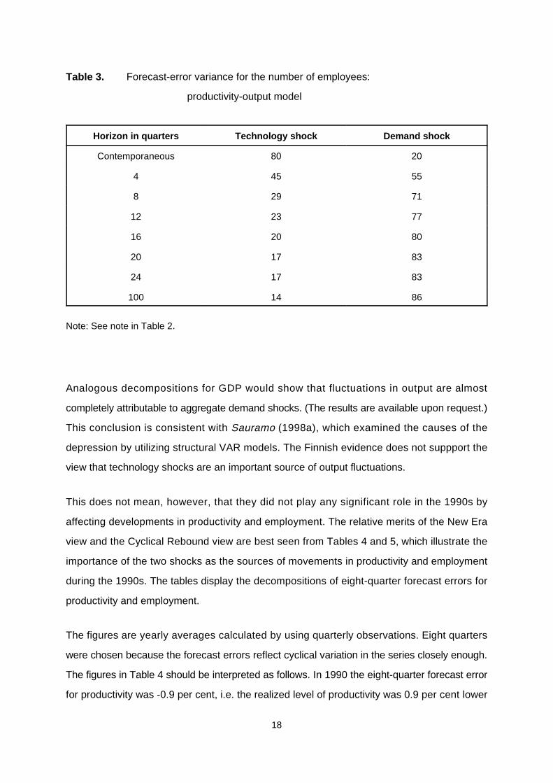
Table 3. Forecast-error variance for the number of employees:

productivity-output model

Horizon in quarters Technology shock Demand shock

Contemporaneous 80 20

4 45 55

8 29 71

12 23 77

16 20 80

20 17 83

24 17 83

100 14 86

Note: See note in Table 2.

Analogous decompositions for GDP would show that fluctuations in output are almost

completely attributable to aggregate demand shocks. (The results are available upon request.)

This conclusion is consistent with Sauramo (1998a), which examined the causes of the

depression by utilizing structural VAR models. The Finnish evidence does not suppport the

view that technology shocks are an important source of output fluctuations.

This does not mean, however, that they did not play any significant role in the 1990s by

affecting developments in productivity and employment. The relative merits of the New Era

view and the Cyclical Rebound view are best seen from Tables 4 and 5, which illustrate the

importance of the two shocks as the sources of movements in productivity and employment

during the 1990s. The tables display the decompositions of eight-quarter forecast errors for

productivity and employment.

The figures are yearly averages calculated by using quarterly observations. Eight quarters

were chosen because the forecast errors reflect cyclical variation in the series closely enough.

The figures in Table 4 should be interpreted as follows. In 1990 the eight-quarter forecast error

for productivity was -0.9 per cent, i.e. the realized level of productivity was 0.9 per cent lower

19

than the forecast by the model. (Owing to the way of computing the forecast errors, they are

not exactly the same as relative forecast errors. See the note in Table 4.) Of this error, +0.9

percentage points was due to the technology shock and -1.8 percentage points to the

aggregate demand shock.

Table 4 shows that at the start of the depression developments of productivity were largely

determined by negative shocks to aggregate demand. The negative figure for 1990 reflects the

effect which Gordon (1993) called "the end-of-expansion effect". The level of productivity

decreases because of overhiring by firms at the stage when output growth has slowed down.

In 1991 the collapse of real output was associated with a strong decline in productivity, which

was caused by a big negative shock to aggregate demand.

For the start of the depression, movements in productivity are largely explained by negative

aggregate demand shocks, whereas technology shocks do not have any role. Developments

at the beginning of the depression are, therefore, in accordance with the Cyclical Rebound

view.

20

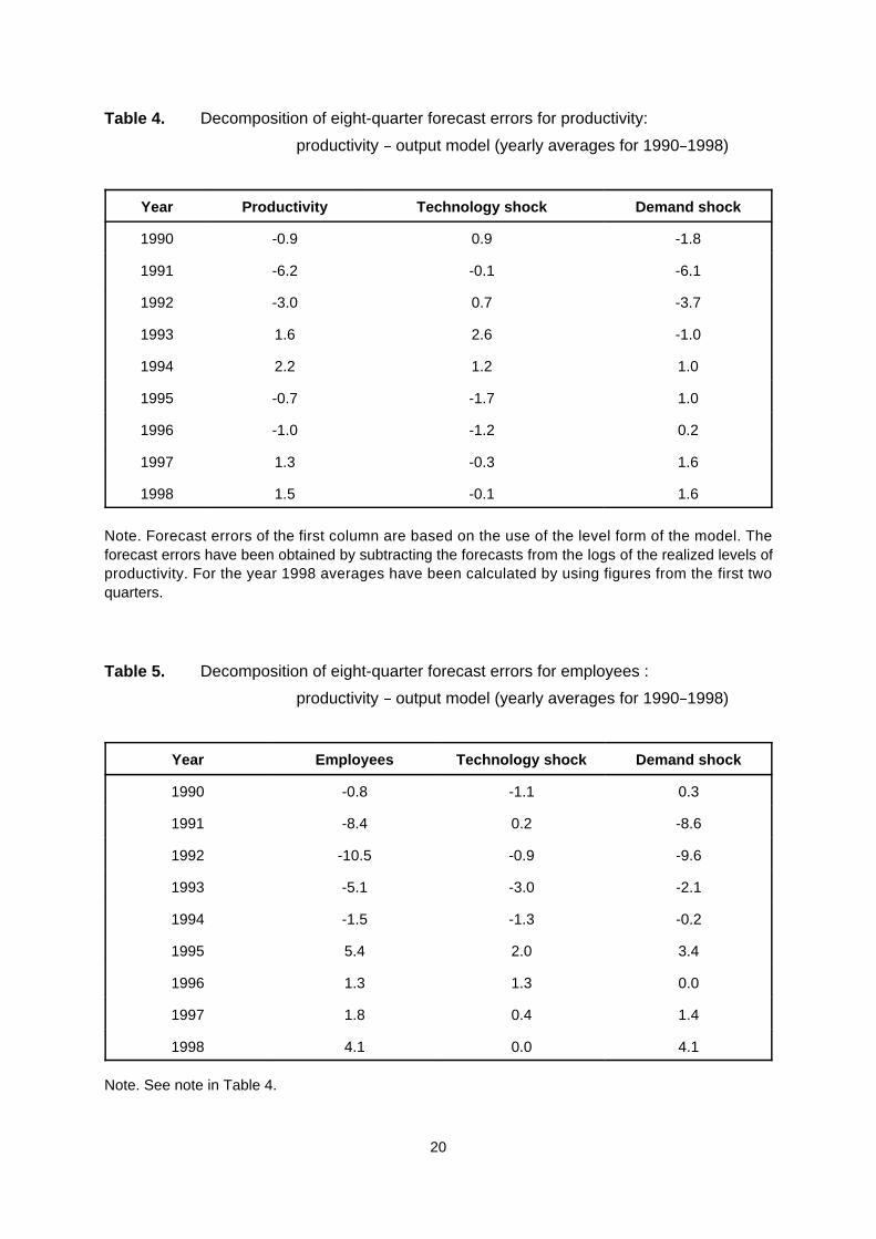
Table 4. Decomposition of eight-quarter forecast errors for productivity:

productivity % output model (yearly averages for 1990%1998)

Year Productivity Technology shock Demand shock

1990 -0.9 0.9 -1.8

1991 -6.2 -0.1 -6.1

1992 -3.0 0.7 -3.7

1993 1.6 2.6 -1.0

1994 2.2 1.2 1.0

1995 -0.7 -1.7 1.0

1996 -1.0 -1.2 0.2

1997 1.3 -0.3 1.6

1998 1.5 -0.1 1.6

Note. Forecast errors of the first column are based on the use of the level form of the model. Theforecast errors have been obtained by subtracting the forecasts from the logs of the realized levels ofproductivity. For the year 1998 averages have been calculated by using figures from the first twoquarters.

Table 5. Decomposition of eight-quarter forecast errors for employees :

productivity % output model (yearly averages for 1990%1998)

Year Employees Technology shock Demand shock

1990 -0.8 -1.1 0.3

1991 -8.4 0.2 -8.6

1992 -10.5 -0.9 -9.6

1993 -5.1 -3.0 -2.1

1994 -1.5 -1.3 -0.2

1995 5.4 2.0 3.4

1996 1.3 1.3 0.0

1997 1.8 0.4 1.4

1998 4.1 0.0 4.1

Note. See note in Table 4.

21

However, during the next stage of the depression the role of technology shocks becomes

important. Because of negative aggregate demand shocks, GDP continued to fall in 1992 and

1993. They also affected the level of productivity negatively, but this effect was neutralized by

positive technology shocks. Even though GDP fell in 1993, productivity increased strongly (see

Table 1). Because of the dominant role of the technological shocks, the pattern was not pro-

but counter-cyclical. Obviously, the developments in 1993 are hard to reconcile with the

Cyclical Rebound view. If any, they are consistent with the New Era view.

In 1994 the economy started to recover and GDP increased by 4.5 per cent. Strong GDP

growth was associated with rapid growth of productivity with both aggregate demand and

technology shocks contributing to the growth.

As a result of rapid growth during the period from 1992 till 1994, productivity reached a level

which was higher than the level predicted by the trend which is obtained by using observations

from the period 1975%1990 (see Figure 1).

The developments can, therefore, be summarized as follows. Because of positive technology

shocks, the productivity trend shifted upwards during the years from 1992 till 1994. However,

the subsequent developments indicate that the rate of productivity growth did not accelerate

permanently (see Figure 1). During the years 1995%1998 increases in productivity have been

consistent with the new trend. Negative technology shocks have, however, neutralized the

upward shift somewhat.

Obviously, neither the New Era view nor the Cyclical Rebound view can explain the

developments in productivity during the 1990s. Also, the developments of employment are hard

to explain by using either of the two views.

As Table 5 illustrates, the sharp fall in employment during the early stage of the depression

was due to adverse aggregate demand shocks. Consistent with Table 4, positive technology

shocks had a negative impact on employment during the years from 1992 till 1994. In 1994,

when GDP was already increasing, employment continued to fall and the rate of unemployment

was still rising (see Table 1). This was mainly due to positive technology shocks. Not

surprisingly, this was the time when the debate about "jobless growth" and "jobless recovery"

22

started. Although the decline in employment in 1994 is consistent with "jobless growth", it is,

however, difficult to connect the subsequent movements in employment with "jobless growth".

The evidence therefore suggests that both the New Era and Cyclical Rebound view provide an

incomplete interpretation about the developments of productivity and employment during the

1990s. Both explain only some specific parts of the developments.

For various interpretations, the years from 1992 till 1994 are the most critical, because during

that period the role of technology shocks was dominant. This means that the definition of a

technology shock becomes crucial. Moreover, because a technology shock is defined as the

only shock which has a permanent influence on the level of productivity, the measure of

productivity is also mirrored in the results.

The exploration was conducted by using a highly aggregative measure of productivity, and,

accordingly, the definition of a technology shock was rationalized by a theoretical model which

was a representative agent model. In the model, households and, what is important, firms were

assumed to be identical. Obviously, that kind of model is not of much use if one wants to

analyse how, for example, business restructuring affects an aggregative measure of

productivity.

In an aggregative analysis, the notion of "technology shock" can be misleading, because

permanent changes in the level of aggregate productivity can result from business restructuring

without including technological improvements at the plant level: the level of aggregate

productivity rises if, as a result of births and deaths, the share of firms with a high level of

productivity rises.

For the interpretation of the results, evidence from relevant studies which utilize plant level data

is therefore valuable. That kind of evidence is available for Finnish manufacturing. Maliranta

(1997) has examined the determinants of the average level of productivity in manufacturing by

employing micro data covering the period from 1975 till 1994. (He utilizes the approach which

Baily, Bartelsman and Haltiwanger, 1996, exploited in their study of the short-run sources of

US productivity.)

23

In Maliranta’s (1997) study, the aggregate labour productivity growth is decomposed into the

following four effects: the entry-exit effect, the share effect, the cross term, and the within plant

effect.

Productivity growth at the plant level seems to have followed the same (log-linear) trend for the

whole period from 1975 to 1994. Within-plant effects, therefore, do not explain changes in the

productivity trend. On the other hand, the results demonstrate that the other three components

have altered productivity growth in manufacturing since the mid-1980s. In particular, the effects

of the micro-structural changes were apparent during the depression.

The entry-exit effect, which describes how the births and deaths of plants affect average

productivity, did contribute to the acceleration of manufacturing productivity growth especially

in 1993 and 1994. This was mainly due to the exit effect, i.e. plants with less than an average

level of productivity disappeared. Also, the share effect, which describes the effects of labour

re-allocation between surviving plants, had a positive contribution notably in 1993. The plants

with an above-average level of productivity therefore increased their labour input share. On the

other hand, the cross-term had a negative contibution, which indicates that the plants with an

above-average rate of productivity growth accounted for a decreasing share of labour input.

Obviously, the positive technology shocks which dominated the developments of aggregate

productivity during the period from 1992 to 1994 also reflect micro-structural changes like

business restructuring and not technological changes at the plant level.

Because of significant entry-exit effects, it is not misleading to characterize the depression as

the period of creative destruction, a characterization Schumpeter (1942) used for recessions.

In Finland the period of creative destruction resulted in an upward shift in the path of trend

productivity. Neither the New Era view nor the Cyclical Rebound view captures this kind of

peculiarity. In contrast to what the New Era view suggests, the rate of trend productivity growth

has not accelerated permanently. However, the change in the development of productivity was

more profound than the Cyclical Rebound view suggests. Furthermore, during the critical years

1992%1993 movements in productivity were counter-cyclical.

24

4. CONCLUSIONS

I have tagged the period of the depression and the subsequent recovery as unusual in that it

resulted in an upward shift in the path of trend productivity. This shift took place during the

years from 1992 to 1994. During that period the relationship between employment growth and

GDP growth was exceptional. In the course of the depression years 1992 and 1993 the decline

in employment was sharper than one would have predicted by using some common rules of

thumb. Moreover, the first year of the recovery, 1994, when GDP grew by 4.5 per cent, was

associated with a further fall in employment.

Within the framework of the paper, the shift, and the unusual connection between employment

and GDP growth, was due to the positive technology shocks which dominated the develop-

ments of productivity and employment. Positive technology shocks lead to a decline in labour

input. The fall in employment as a result of a positive technology shock is consistent with

predictions by a broad class of sticky price models which served as the theoretical background

of the investigation.

According to the results it is not correct to say that the Finnish economy has moved into a New

Era which is characterized by a faster-than-before rate of productivity growth. In any case, it

experienced a period which was characterized by "jobless growth", the source of "joblessness"

being positive technology shocks. In the latter part of the 1990s, productivity growth has

evened out, however. Furthermore, during the period from 1992 to 1994 movements in

productivity did not obey the usual pro-cyclical pattern. The upward shift of the productivity

trend cannot, therefore, easily be interpreted as the usual Cyclical Rebound.

The examination was based on the use of a highly aggregative measure of productivity (real

GDP per employee), which, of course, makes the interpretation of the results less clearcut.

Rather than reflecting within-plant improvements in technology, the technology shocks may

reflect business restructuring. For Finnish manufacturing, there is evidence which supports that

kind of interpretation. Even though it may be a more adequate interpretation, it would not

weaken the main conclusion to be drawn from the results: the period from 1992 to 1994 was

25

exceptional, and, furthermore, exceptionality is hard to describe by utilizing either the New Era

or Cyclical Rebound view.

However, in order to refine the main conclusion, more work should be done. A natural way of

extending the exploration of this paper is to use more disaggregated data. (For that kind of

investigation, see Malley and Muscatelli, 1997 and Malley, Muscatelli and Woitek, 1998.) The

use of industry-level data should turn out to be useful, because movements in productivity have

varied considerably across industries. Even though the construction of reliable quarterly data

on productivity for various industries is not straightforward, such data can be constructed. The

use of such data enables one to study whether the upward shift in the trend path of aggregate

productivity only mirrors changes in manufacturing or whether it is apparent in other industries,

too.

Additional studies which are based on micro data would, of course, be invaluable. This study

illustrates the fact that relying solely on the use of aggregate data can lead to misinter-

pretations.

26

REFERENCES

Baily, M.N., E.J. Bartelsman and J. Haltiwanger (1996), Labor Productivity:Structural Change and Cyclical Factors, NBER Working Paper 5503.

Basu, S., J. Fernald and M. Kimball (1998), Are Technology ImprovementsContractionary? International Finance Discussion Papers No 625, Board of Governors of theFederal Reserve System, Washington DC.

Blanchard, O. J. and D. Quah (1989), The Dynamic Effects of Aggregate Demandand Supply Disturbances, American Economic Review, 79, 655%673.

Castillo, S., J. J. Dolado and J. F. Jimeno (1998), The tale of two neighboureconomies: labour market dynamics in Spain and Portugal, CEPR Discussion paper series No.1954, London.

Dolado, J. J. and J. F. Jimeno (1997), The causes of Spanish unemployment: Astructural VAR approach. European Economic Review, 41, 1281%1307.

Gali, J. (1999), Technology, Employment, and the Business Cycle: DoTechnology Shocks Explain Aggregate Fluctuations?, American Economic Review, 89,249%271.

Gali, J. and M. L. Hammour (1991), Long run effects of business cycles, mimeo,Columbia University, New York.

Gordon, R. J. (1993), The Jobless Recovery: Does It Signal a New Era ofProductivity-led Growth?, Brookings Papers on Economic Activity, 1:1993, 271%306.

Jacobson, T., A. Vredin, and A. Warne (1997), Common Trends and Hysteresisin Unemployment, European Economic Review, 41, 1781%1816.

Jacobson, T., A. Vredin and A. Warne (1998), Are Real Wages andUnemployment Related?, Economica, 65, 69-96.

Kahn, G. A. (1993), Sluggish Job Growth: Is Rising Productivity or an AnemicRecovery To Blame?, Federal Reserve Bank of Kansans City Economic Review Third Quarter5%25.

Maliranta, M. (1997), Plant Level Explanations for the Catch Up Process inFinnish Manufacturing: A Decomposition of Aggregate Labour Productivity Growth, inLaaksonen, S. (ed.), The Evolution of Firms and Industries, Research Reports 223, StatisticsFinland, Helsinki.

Malley, J. and V.A. Muscatelli (1997), Productivity shocks and employment:evidence from US industrial data, Economics Letters, 57, 97%105.

27

Malley, J.R., V.A. Muscatelli and U. Woitek (1998), The Interaction BetweenBusiness Cycles and Productivity Growth: Evidence from US Industrial Data, University ofGlasgow, Discussion Papers in Economics No 9805, Glasgow.

OECD (1994), The OECD Jobs Study: Evidence and Explanations, Part I %Labour Market Trends and Underlying Forces of Change, Paris.

Sauramo, P. (1998a), The Boom and the Depression: An Analysis within theAggregate-Demand % Aggregate-Supply Framework, Discussion papers 143, Labour Institutefor Economic Research, Helsinki.

Sauramo, P. (1998b), The Boom and the Depression: A Note on the Identificationof Aggregate Supply Shocks, Discussion papers 147, Labour Institute for Economic Research,Helsinki.

Schumpeter, J. A. (1942), Capitalism, Socialism and Democracy, New York.

28

Palkansaajien tutkimuslaitos / Labour Institute for Economic Research

Tutkimusselosteita / Discussion Papers (ISSN 1236 %7184)

123 Kaj Ilmonen, Työmarkkinajärjestelmä, talouden kansainvälistyminen ja ay-liike, 1995.

124 Jukka Pekkarinen, Keynes ja velkadeflaatio, 1995.

125 Juhana Vartiainen, Can Nordic social corporatism survive? Challenges to the LabourMarket, 1995.

126 Seppo Toivonen, Kiinteistöveron käyttö lähiöiden perusparannushankkeiden rahoituk-sessa, 1995.

127 Hannu Piekkola, Taxation under economic integration, 1996.

128 Petri Böckerman, Tanskan pitkäaikaistyöttömyys ja sen hoitokeinot, 1996.

129 Mari Kangasniemi, Työmarkkinoiden polarisoituminen: Kirjallisuuskatsaus, 1996.

130 Petri Böckerman, Ansiotyösidonnaisista tukijärjestelmistä saadut kansainvälisetkokemukset, 1996.

131 Petri Böckerman, Työsopimukset, organisaatiorakenne ja tuottavuus, 1996

132 Pekka Sauramo, The boom and the depression % A simple shock interpretation, 1996.

133 Seija Ilmakunnas, Child care costs in labour supply models, 1996.

134 Eero Lehto, Group versus piece-rate contract, 1996.

135 Eero Lehto, Two-wage schemes, frequently observed output and a team contract,1996.

136 Petri Böckerman, Ansiosidonnainen tukijärjestelmä Suomen kannalta, 1997.

137 Katri Kosonen, House price dynamics in Finland, 1997.

138 Pasi Holm, Jaakko Kiander & Pekka Tossavainen, Rahastot ja EMU, 1997.

139 Katri Kosonen, Investment in residential building: A time-series, 1997.

140 Jukka Pekkarinen, Markan kelluttaminen talouspoliittisena vaihtoehtona EMUntoteuduttua, 1997.

141 Pertti Haaparanta & Hannu Piekkola, Rent-Sharing Financial Pressures and FirmBehavior, 1997.

142 Petri Böckerman, Regional evolutions in Finland, 1998.

29

143 Pekka Sauramo, The Boom and the Depression: An Analysis within the AggregateDemand%Aggregate-Supply Framework, 1998.

144 Tuomas Pekkarinen, The Wage Curve: Finnish Evidence, 1998.

145 Petri Böckerman, Työn jakaminen ja työllisyys, 1998.

146 Petri Böckerman & Jaakko Kiander, Työllisyys Suomessa 1960%1996, 1998.

147 Pekka Sauramo, The Boom and the Depression: A Note on the Identification ofAggregate Supply Shocks, 1998.

148 Petri Böckerman & Jaakko Kiander, Has work-sharing worked in Finland?, 1998.

149 Petri Böckerman, Asuntomarkkinoiden toiminta ja työmarkkinoiden sopeutuminen,1998.

150 Petri Böckerman, Asuntokysyntä Suomessa. Poikkileikkaustarkastelu käyttäenvarallisuustutkimusta 1994, 1999.

151 Markus Jäntti & Sheldon Danziger, Income Poverty in Advanced Countries, 1999.

152 Jaakko Kiander, Työajan lyhentäminen ja työllisyys, 1999.

153 Petri Böckerman, Työn tarjonta ja työttömyys alue-ennusteessa, 1999.

154 Hannu Piekkola & Satu Hohti & Pekka Ilmakunnas, Experience and productivity inwage formation in Finnish industries, 1999.

155 Juhana Vartiainen, Job assignment and the general wage differential: Theory andevidence on Finnish metalworkers, 1999.

156 Juhana Vartiainen, Relative wages in monetary Union and floating, 1999.

157 Petri Böckerman & Jaakko Kiander, Determination of average working time inFinland, 1999.

158 Kimmo Kevätsalo & Kaj Ilmonen & Kari Jokivuori, Sopiminen, luottamus jatoimipaikkakoko, 1999.

159 Pekka Sauramo, Jobless growth in Finland? Evidence from the 1990s, 1999.