Liquidity Traps and Jobless Recoveries - Columbia Universitymu2166/Making_Contraction/paper.pdf · Liquidity Traps and Jobless Growth Recoveries in the United States, ... liquidity

American Economic Journal: Macroeconomics 2017, 9(1): 165–204 https://doi.org/10.1257/mac.20150220

165

Liquidity Traps and Jobless Recoveries†

By Stephanie Schmitt-Grohé and Martín Uribe*

This paper proposes a model that explains the joint occurrence of liquidity traps and jobless growth recoveries. Its key elements are downward nominal wage rigidity, a Taylor-type interest rate feedback rule, the zero lower bound on nominal interest rates, and a confidence shock. Absent a change in policy, the model predicts that low inflation and high unemployment become chronic. With capital accumulation, the model predicts, in addition, an investment slump. The paper identifies a New Fisherian effect, whereby raising the nominal interest rate to its intended target for an extended period of time can boost inflationary expectations and thereby foster employment. (JEL E24, E31, E32, E43, E52, F44, G01)

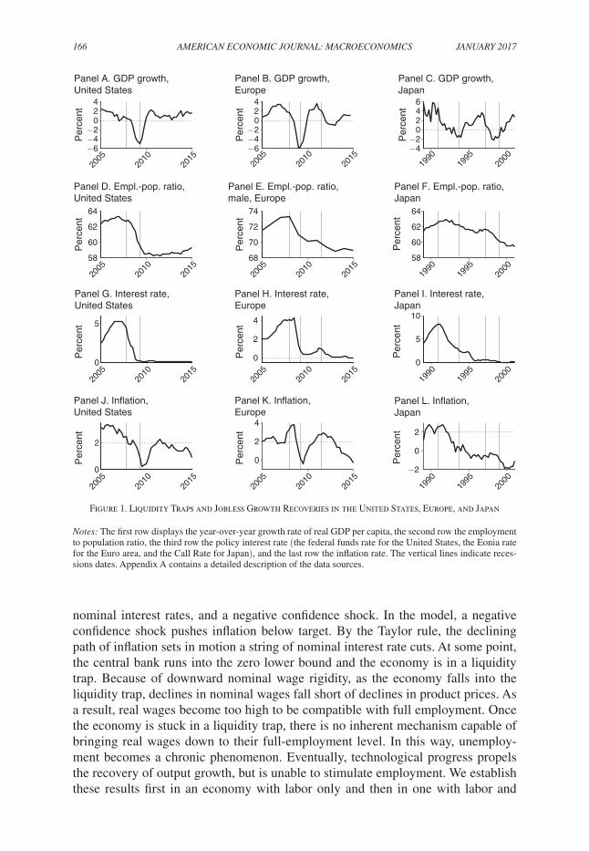
The Great Contractions in Europe and the United States in 2008 were accompa-nied by zero nominal interest rates and inflation below target. A further nota-

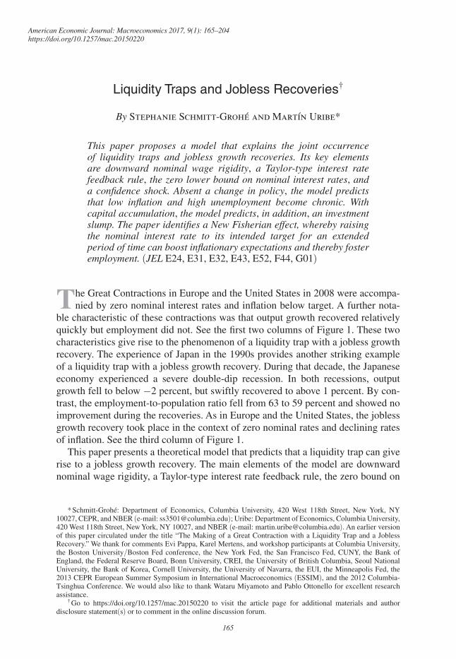
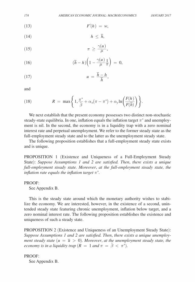
ble characteristic of these contractions was that output growth recovered relatively quickly but employment did not. See the first two columns of Figure 1. These two characteristics give rise to the phenomenon of a liquidity trap with a jobless growth recovery. The experience of Japan in the 1990s provides another striking example of a liquidity trap with a jobless growth recovery. During that decade, the Japanese economy experienced a severe double-dip recession. In both recessions, output growth fell to below −2 percent, but swiftly recovered to above 1 percent. By con-trast, the employment-to-population ratio fell from 63 to 59 percent and showed no improvement during the recoveries. As in Europe and the United States, the jobless growth recovery took place in the context of zero nominal rates and declining rates of inflation. See the third column of Figure 1.

This paper presents a theoretical model that predicts that a liquidity trap can give rise to a jobless growth recovery. The main elements of the model are downward nominal wage rigidity, a Taylor-type interest rate feedback rule, the zero bound on

* Schmitt-Grohé: Department of Economics, Columbia University, 420 West 118th Street, New York, NY10027, CEPR, and NBER (e-mail: [email protected]); Uribe: Department of Economics, Columbia University, 420 West 118th Street, New York, NY 10027, and NBER (e-mail: [email protected]). An earlier version of this paper circulated under the title “The Making of a Great Contraction with a Liquidity Trap and a Jobless Recovery.” We thank for comments Evi Pappa, Karel Mertens, and workshop participants at Columbia University, the Boston University/Boston Fed conference, the New York Fed, the San Francisco Fed, CUNY, the Bank ofEngland, the Federal Reserve Board, Bonn University, CREI, the University of British Columbia, Seoul National University, the Bank of Korea, Cornell University, the University of Navarra, the EUI, the Minneapolis Fed, the 2013 CEPR European Summer Symposium in International Macroeconomics (ESSIM), and the 2012 Columbia-Tsinghua Conference. We would also like to thank Wataru Miyamoto and Pablo Ottonello for excellent research assistance.

† Go to https://doi.org/10.1257/mac.20150220 to visit the article page for additional materials and author disclosure statement(s) or to comment in the online discussion forum.

166 AMErIcAN EcoNoMIc JourNAL: MAcroEcoNoMIcs JANuAry 2017

nominal interest rates, and a negative confidence shock. In the model, a negative confidence shock pushes inflation below target. By the Taylor rule, the declining path of inflation sets in motion a string of nominal interest rate cuts. At some point, the central bank runs into the zero lower bound and the economy is in a liquidity trap. Because of downward nominal wage rigidity, as the economy falls into the liquidity trap, declines in nominal wages fall short of declines in product prices. As a result, real wages become too high to be compatible with full employment. Once the economy is stuck in a liquidity trap, there is no inherent mechanism capable of bringing real wages down to their full-employment level. In this way, unemploy-ment becomes a chronic phenomenon. Eventually, technological progress propels the recovery of output growth, but is unable to stimulate employment. We establish these results first in an economy with labor only and then in one with labor and

Figure 1. Liquidity Traps and Jobless Growth Recoveries in the United States, Europe, and Japan

Notes: The first row displays the year-over-year growth rate of real GDP per capita, the second row the employment to population ratio, the third row the policy interest rate (the federal funds rate for the United States, the Eonia rate for the Euro area, and the Call Rate for Japan), and the last row the inflation rate. The vertical lines indicate reces-sions dates. Appendix A contains a detailed description of the data sources.

2005

2010

2015

2005

2010

2015

2005

2010

2015

2005

2010

2015

−6−4−2

024

−6−4−2

024

Per

cent

Per

cent

Per

cent

Per

cent

Per

cent

Per

cent

Per

cent

Per

cent

Per

cent

Per

cent

Per

cent

Per

cent

Panel A. GDP growth, United States

58

60

62

64

Panel D. Empl.-pop. ratio, United States

0

5

Panel G. Interest rate, United States

0

2

Panel J. Inflation, United States

2005

2010

2015

2005

2010

2015

2005

2010

2015

2005

2010

2015

Panel B. GDP growth, Europe

68

70

72

74

Panel E. Empl.-pop. ratio, male, Europe

0

2

4

Panel H. Interest rate, Europe

0

2

4

Panel K. Inflation, Europe

1990

1995

2000

1990

1995

2000

1990

1995

2000

1990

1995

2000

−4 −2

0246

Panel C. GDP growth, Japan

58

60

62

64

Panel F. Empl.-pop. ratio, Japan

0

5

10

Panel I. Interest rate, Japan

−2

0

2

Panel L. Inflation, Japan

VoL. 9 No. 1 167Schmitt-Grohé and Uribe: LiqUidity trapS and JobLeSS recoverieS

capital accumulation. In the economy with capital, the jobless growth recovery is accompanied by an investment slump.

Our emphasis on the role of a confidence shock to explain the joint occurrence of a liquidity trap and a jobless growth recovery appears to be supported by economet-ric studies of the Japanese case. Aruoba, Cuba-Borda, and Schorfheide (2014), for example, estimate a model with fundamental and non-fundamental shocks. Using data from Japan, they find that this country experienced a confidence-shock-driven switch to a deflation regime in 1999 and has remained there ever since.

The equilibrium dynamics implied by the model presented here are quite dif-ferent in response to fundamental shocks. When inflationary expectations are well anchored (i.e., in the absence of confidence shocks), inflationary expectations con-verge quickly to the central bank’s intended inflation target as the negative funda-mental shock fades away. As inflation converges to its target level, it erodes the real purchasing power of wages, fostering employment. Consequently, the recov-ery from a contraction driven by fundamental shocks is characterized by both an increase in output growth and, more importantly, job creation.

An important policy challenge is how to revive job creation in an economy that is stuck in a liquidity trap. Most academic and professional economists agree that an essential element to bring an economy out of a liquidity trap is to raise inflationary expectations (see, for example, Krugman 1998, Woodford 2012). However, what policy is able to raise inflationary expectations in a liquidity trap depends upon the nature of the shock that pushed the economy into the liquidity trap in the first place. Eggertsson and Woodford (2003) show that if the underlying shock is fundamental (in particular a fall in the natural rate), then inflationary expectations can be lifted by promising to keep nominal rates at zero for an extended period of time, even after the shock has dissipated. In the present paper, we establish that, while this prescription works well for fundamental shocks, it may not work equally well if the root cause of the slump is a non-fundamental confidence shock. In this situation, a promise of low interest rates for a prolonged period of time validates low inflation expectations and in this way perpetuates the slump. The reason a policy of low inter-est rates for an extended period of time cannot generate expected inflation when the liquidity trap is the result of a confidence shock is that in these circumstances the negative relationship between nominal interest rates and inflationary expectations ceases to be valid and might indeed reverse sign.

During normal times, that is, when inflationary expectations are well anchored around the intended target, the primary effect of an increase in nominal interest rates is a decline in inflation via a fall in aggregate demand. Similarly, under normal circumstances, a reduction of the nominal interest rate tends to boost short-run infla-tionary expectations through an elevated level of aggregate spending. In contrast, in a liquidity trap driven by lack of confidence, the sign is reversed. Low interest rates are not accompanied by high levels of inflation but rather by falling or even negative inflation. Moreover, because the economy is already inundated by liquidity, a fall in interest rates has no longer a stimulating effect on aggregate demand. An insight that emerges from the present paper is that the reversal of sign in the relationship between interest rates and expected inflation also operates in the upward direction. That is, that in a liquidity trap caused by a confidence shock, an increase in nominal


rates tends to raise inflationary expectations without further depressing aggregate spending. It follows from this insight that any policy that is to succeed in raising inflationary expectations during an expectations-driven liquidity trap must be asso-ciated with an increase in nominal rates.

Accordingly, the paper presents an interest-rate-based strategy for escaping liquidity traps. Specifically, this strategy stipulates that when inflation falls below a threshold, the central bank temporarily deviates from the traditional Taylor rule by pegging the nominal interest rate at the target level until inflation returns to its intended target level. The paper shows that this policy, rather than exacerbating the recession as conventional wisdom would have it, can boost inflationary expec-tations and thereby lift the economy out of the slump. The sustained increase in the nominal interest rate generates conditions for economic recovery because of a Fisherian effect positively linking expected inflation to the nominal interest rate and a Keynesian effect negatively linking inflation to real wage growth.

This paper is related to a body of work on liquidity traps. The theoretical frame-work extends the work of Benhabib, Schmitt-Grohé, and Uribe (2001) by incor-porating downward nominal wage rigidity and involuntary unemployment. Shimer (2012) shows that in a real search model with real wage rigidity, recoveries can be jobless. The present model differs from Shimer’s in two important aspects. First, the model assumes that nominal wages are downwardly rigid, but real wages are flexible. The assumption of nominal rather than real wage rigidity is motivated by an empirical literature suggesting that the former type of rigidity is pervasive (see, for instance, Gottschalk 2005; Barattieri, Basu, and Gottschalk 2014; and Daly, Hobijn, and Lucking 2012 for the United States; Holden and Wulfsberg 2008, and Schmitt-Grohé and Uribe 2016 for the euro area and Argentina; and Kuroda and Yamamoto 2003 for Japan). Second, in real models of jobless recoveries, monetary policy plays no role by construction. By contrast, a central prediction of the current formulation is that monetary policy plays a crucial role in determining whether a recovery is jobless or not. Indeed, there is empirical evidence showing that the stance of monetary policy does matter for labor market outcomes in recoveries (Calvo, Coricelli, and Ottonello 2012). Mertens and Ravn (2014) study the size of fiscal multipliers in a version of the Benhabib, Schmitt-Grohé, and Uribe (2001) model. They find that the size of the fiscal multiplier associated with a particu-lar fiscal instrument depends on the type of shock that pushed the economy into the liquidity trap. In particular, they show that when the liquidity trap is due to a non-fundamental shock, supply-side fiscal instruments have a large multiplier, and demand-side fiscal instruments have a small multiplier. The reverse is true when the liquidity trap is caused by a fundamental shock. Cochrane (2014) shows that an increase in the nominal interest rate can increase inflationary expectations in a policy regime characterized by passive monetary policy and active fiscal policy. This paper is also related to a recent literature on secular stagnation. In this class of models, long recessions are characterized by low or negative real interest rates, see in particular the formulations by Eggertsson and Mehrotra (2014) and Benigno and Fornaro (2015). In the former, low real interest rates are due to shocks that affect savings over the life cycle and in the latter to an endogenous fall in firms’ technological innovation.


The remainder of the paper is organized in seven sections. Section I presents the model. Section II shows that the model possesses two steady states, one with zero unemployment and inflation equal to its target level, and one with involuntary unemployment and zero nominal rates. Section III shows that a lack-of-confidence shock leads to a recession, a liquidity trap, and a jobless growth recovery. Section IV shows that in response to a fundamental decline in the natural rate, the recovery fea-tures job creation. Section V shows that raising nominal rates can lift the economy out of a confidence-shock-induced liquidity trap without much initial costs in terms of output or unemployment. Section VI shows that the results of the paper are robust to allowing for capital accumulation. Section VII concludes.

I. The Model

Consider an economy populated by a large number of infinitely lived households with preferences described by the utility function

(1) E 0 ∑ t=0

∞

e ξ t β t u( c t ),

where c t denotes consumption, ξ t is an exogenous taste shock with mean zero, β ∈ (0, 1 ) is a subjective discount factor, and E t is the expectations operator condi-tional on information available in period t . We assume that the period utility function takes the form

u(c ) = c 1−σ − 1 _ 1 − σ ,

with σ > 0 .Households are assumed to be endowed with a constant number of hours,

denoted h , which they supply inelastically to the labor market. Because of the pres-ence of nominal wage rigidity, households will in general be able to sell only h t ≤ h hours each period, where h t is endogenously determined in equilibrium, but taken as exogenous by the individual agent. Households pay nominal lump sum taxes in the amount T t , receive nominal profits from the ownership of firms in the amount Φ t , and trade in a nominally risk-free bond, denoted B t , that pays the gross nominal interest rate r t . The budget constraint of the household is then given by

(2) P t c t + B t = W t h t + r t−1 B t−1 + Φ t − T t ,

where P t and W t denote, respectively, the nominal price level and the nominal wage rate in period t .

In each period t ≥ 0 , the optimization problem of the household consists in choosing c t and B t to maximize (1), subject to the budget constraint (2), and to a no-Ponzi-game constraint of the form lim j→∞ E t ( ∏ s=0

j r t+s −1 ) B t+j+1 ≥ 0 . The


optimality conditions associated with this maximization problem are the budget constraint (2), the no-Ponzi-game constraint holding with equality, and

e ξ t u ′ ( c t ) = β r t E t [ e ξ t+1 u ′ ( c t+1 ) _ π t+1 ] ,

where π t ≡ P t / P t−1 denotes the gross rate of inflation in period t .Consumption goods are produced by competitive firms using labor as the sole

input via the technology

y t = X t F( h t ),

where y t denotes output, and X t denotes a deterministic trend in productivity that evolves according to

X t = μ X t−1 ,

where μ > 0 is a parameter. We assume that the production function takes the form

F(h) = h α ,

with α ∈ (0, 1) . Firm profits are given by

Φ t = P t X t F( h t ) − W t h t .

The firm chooses h t to maximize Φ t . The associated optimality condition is

X t F ′ ( h t ) = W t _ P t .

According to this expression, firms are always on their labor demand curve. As we will see shortly, this will not be the case for workers, who will sometimes be off their labor supply schedule and will experience involuntary unemployment.

A. Downward Nominal Wage rigidity

Nominal wages are assumed to be downwardly rigid. Specifically, in any given period, nominal wage growth is bounded below by γ( u t ) ,

W t _ W t−1 ≥ γ( u t ),

where the function γ ( u t ) is assumed to be positive and u t ≡ ( h − h t )/ h denotes the aggregate rate of unemployment. The variable u t is meant to capture involuntary unemployment above the natural rate. This setup nests the cases of


absolute downward wage rigidity, when γ ( u t ) ≥ 1 for all u t , and full wage flex-ibility when γ ( u t ) = 0 for all u t . We impose the following assumption on the function γ( · ) .

ASSUMPTION 1: The function γ ( u t ) satisfies

γ′( u t ) < 0,

and

γ (0) > β μ,

where β ≡ β μ −σ .

The first condition in Assumption 1 allows for nominal wages to become more flexible as unemployment increases. The second condition says that in periods of full employment, nominal wage growth cannot fall too much below the rate of labor productivity growth. We will see that this restriction is necessary to ensure the uniqueness of the full-employment steady state and the existence of a second steady state with involuntary unemployment. In the simulations reported below, we assume that γ (u) takes the form

γ (u) = γ 0 (1 − u ) γ 1 ,

with γ 0 , γ 1 > 0 .The presence of downwardly rigid nominal wages implies that the labor market

will in general not clear at the inelastically supplied level of hours h . Instead, invol-untary unemployment, given by h − h t , will be a regular feature of this economy. Actual employment must satisfy

h t ≤ h

at all times. Finally, we impose the following slackness condition on wages and employment:

( h − h t ) ( W t − γ ( u t ) W t−1 ) = 0.

This condition implies that whenever there is involuntary unemployment, the lower bound on nominal wages must be binding. It also says that whenever the lower bound on nominal wages does not bind, the economy must be operating at full employment.


B. The Government

The government is assumed to levy lump sum taxes and issue public debt. Public consumption is assumed to be nil. The sequential budget constraint of the govern-ment is then given by

B t + T t = r t−1 B t−1 .

We assume that lump sum taxes are chosen to ensure the government’s solvency at all times and for any path of the price level. One such fiscal policy would be, for instance, to set T t endogenously at a level such that B t = 0 for all t .

Monetary policy takes the form of a Taylor-type feedback rule, whereby the gross nominal interest rate is set as an increasing function of inflation and the output gap. Specifically, we assume that the interest rate rule is of the form

r t = max {1, r ∗ + α π ( π t − π ∗ ) + α y ln ( y t _ y t ∗

) } ,

where π ∗ denotes the gross inflation target, and r ∗ , α π , and α y are positive coeffi-cients. The variable y t ∗ denotes the flexible-wage level of output. That is,

y t ∗ = X t h α .

The interest rate rule is bounded below by unity to satisfy the zero bound on nominal interest rates. We introduce the following assumption involving the parameters of the Taylor rule.

ASSUMPTION 2: The parameters r ∗ , π ∗ , and α π satisfy

r ∗ ≡ π ∗ _ β > 1,

α π β > 1,

and

π ∗ > γ(0 ) _ μ .

The first two conditions are quite standard. The first one allows the inflation target, π ∗ , to be supported as a deterministic steady state equilibrium. The second one is known as the Taylor principle and guarantees local uniqueness of equilibrium in the neighborhood of a steady state with full employment and inflation at target (the intended steady state). The third condition is needed for the existence of a unique full-employment steady-state equilibrium.


C. Equilibrium

In equilibrium, the goods market must clear. That is, consumption must equal production:

c t = X t F( h t ).

To facilitate the characterization of equilibrium, we scale all real variables that dis-play long-run growth by the deterministic productivity trend X t . Specifically, let c t ≡ c t / X t and w t ≡ W t / ( P t X t ) . Then, the competitive equilibrium is defined as a set of processes { c t , h t , u t , w t , π t , r t } t=0 ∞ satisfying

(3) e ξ t c t −σ = β r t E t [ e ξ t+1 c t+1 −σ _ π t+1 ] ,

(4) c t = F( h t ) ,

(5) F ′ ( h t ) = w t ,

(6) h t ≤ h ,

(7) w t ≥ γ( u t ) _ μ w t−1 _ π t ,

(8) ( h − h t ) ( w t − γ( u t ) _ μ w t−1 _ π t ) = 0 ,

(9) u t = h − h t _ h ,

and

(10) r t = max {1, π ∗ _

β + α π ( π t − π ∗ ) + α y ln ( F( h t ) _

F( h ) ) } ,

given the exogenous process { ξ t } t=0 ∞ and the initial condition w −1 .

II. Non-stochastic Steady-State Equilibria

Non-stochastic steady-state equilibria are equilibria in which all endogenous and exogenous variables are constant over time. Formally, a non-stochastic steady state is a set of constant sequences ξ t = 0 , c t = c , h t = h , w t = w , r t = r , u t = u , and π t = π for all t satisfying

(11) r = π _ β ,

(12) c = F(h) ,


(13) F ′ (h ) = w ,

(14) h ≤ h ,

(15) π ≥ γ(u ) _ μ ,

(16) ( h − h ) (1 − γ(u ) _ μ 1 _ π ) = 0 ,

(17) u = h − h _ h ,

and

(18) r = max {1, π ∗ _

β + α π (π − π ∗ ) + α y ln ( F(h )

_ F( h )

) } .

We next establish that the present economy possesses two distinct non-stochastic steady-state equilibria. In one, inflation equals the inflation target π ∗ and unemploy-ment is nil. In the second, the economy is in a liquidity trap with a zero nominal interest rate and perpetual unemployment. We refer to the former steady state as the full-employment steady state and to the latter as the unemployment steady state.

The following proposition establishes that a full-employment steady state exists and is unique.

PROPOSITION 1 (Existence and Uniqueness of a Full-Employment Steady State): suppose Assumptions 1 and 2 are satisfied. Then, there exists a unique full-employment steady state. Moreover, at the full-employment steady state, the inflation rate equals the inflation target π ∗ .

PROOF:See Appendix B.

This is the steady state around which the monetary authority wishes to stabi-lize the economy. We are interested, however, in the existence of a second, unin-tended steady state featuring chronic unemployment, inflation below target, and a zero nominal interest rate. The following proposition establishes the existence and uniqueness of such a steady state.

PROPOSITION 2 (Existence and Uniqueness of an Unemployment Steady State): suppose Assumptions 1 and 2 are satisfied. Then, there exists a unique unemploy-ment steady state ( u = u > 0 ). Moreover, at the unemployment steady state, the economy is in a liquidity trap ( r = 1 and π = β < π ∗ ).



The existence of two non-stochastic steady states, one in which the inflation rate equals the inflation target and one in which the economy is in a liquidity trap is in line with Benhabib, Schmitt-Grohé, and Uribe (2001). However, a key difference is that in the present environment, the unintended steady state features involuntary unem-ployment, which potentially can make this steady state highly undesirable in terms of welfare. Suppose, for example, that the unemployment rate in the unintended steady state is 5 percent ( u = 0.05 ) higher than the natural rate, which, as we will argue later, is consistent with a plausible calibration of the model. Suppose further that the labor share, α , equals 0.75. Then, we have that consumption at the unintended steady state would be 3.75 percent lower than at the intended steady state. This represents a large decline in consumption in the sense that welfare costs of business cycles are often estimated to be less than one-tenth of 1 percent of consumption.

III. Great Contractions with Jobless Recoveries

Consider equilibria driven by revisions in inflationary expectations. We have in mind situations in which, because of a loss of confidence, the rate of inflation is below expectations. We will show that such a non-fundamental demand shock results in dynamics leading to inflation below target, unemployment, and falling nominal interest rates, and, eventually, the unintended steady state. More impor-tantly, these dynamics will be shown to display a jobless recovery in the sense that output growth returns to normal but unemployment lingers.

Suppose that prior to period 0, the economy was in a steady state with full employment, u −1 = 0 , and an inflation rate equal to the policy target, π −1 = π ∗ . Furthermore, assume that in period − 1 , agents expected π 0 to equal π ∗ . Suppose that in period 0, a negative revision in agents’ economic outlook causes the rate of inflation π 0 to fall below the expected level π ∗ . Assume that from period 0 on, infla-tionary expectations are always fulfilled and that there are no shocks to economic fundamentals. The following proposition establishes that inflation falls monotoni-cally below a threshold and then remains below this threshold forever.

PROPOSITION 3 (Inflation Dynamics under Lack of Confidence): suppose Assumptions 1 and 2 are satisfied, ξ t = 0 and deterministic for t ≥ 0 , and π 0 < π ∗ . Then, in any perfect foresight equilibrium,

π t+1 ⎧

⎪

⎨ ⎪

⎩ < π t < π ∗

if π t ≥ γ(0)

_ μ

< γ(0) _ μ < π ∗

if π t < γ(0)

_ μ , for all t ≥ 0.

Furthermore, there exists a finite date T ≥ 0 such that π T < γ(0 ) _ μ .


The significance of the inflation threshold γ (0)/μ is that once inflation falls below it, full employment becomes impossible. The reason is that because of the


downward rigidity of nominal wages, the ratio γ (0)/ π t represents a lower bound on real wage growth under full employment. If this ratio exceeds the growth rate of productivity, μ , then it must be that real wages are growing at a rate larger than μ . But under full employment, wages cannot grow at a rate exceeding μ , since X t F ′ ( h ) can grow at most at the rate μ . Therefore, if inflation falls below the thresh-old γ(0)/μ , the economy must experience involuntary unemployment. Because the Taylor rule is unable to bring the rate of inflation above the threshold γ (0)/μ , the presence of unemployment becomes chronic. We establish this result in the follow-ing proposition.

PROPOSITION 4 (Chronic Involuntary Unemployment under Lack of Confidence): suppose Assumptions 1 and 2 are satisfied, ξ t = 0 and deterministic for t ≥ 0 , and π 0 < π ∗ . Then, in any perfect foresight equilibrium u t > 0 for all t ≥ T , where T ≥ 0 is the finite integer defined in Proposition 3.


Given an initial rate of inflation π 0 < π ∗ , a perfect-foresight equilibrium can be shown to exist and to be unique. The following proposition formalizes this result.

PROPOSITION 5 (Existence and Uniqueness of Chronic Unemployment Equilibria): suppose Assumptions 1 and 2 are satisfied, ξ t = 0 and deterministic for t ≥ 0 , and w −1 = F ′ ( h ) . Then, given π 0 < π ∗ there exists a unique perfect foresight equilibrium.


The intuition for the existence of equilibria in which expectations of future increases in unemployment are self-fulfilling could be as follows. Suppose in period t agents expect unemployment in period t + 1 to be higher. This change in expec-tations represents a negative income shock to the household as future labor income is expected to decline. This decline in income lowers desired consumption in all periods. Lower demand in period t leads to lower prices in period t . In turn, a decline in current inflation, by the Taylor rule, reduces the current nominal interest rate. And a lower nominal interest rate, as long as expected inflation does not fall by as much as the current nominal rate, causes the real interest rate to decline. The fall in the real interest rate induces a declining path in consumption. In this way, demand next period is weaker than demand today, validating the initial expectation of higher future unemployment.

Importantly, if the dynamics triggered by the initial revision in inflationary expec-tations converge, the convergence point is the unemployment steady state, charac-terized in Proposition 2, featuring involuntary unemployment and a zero nominal interest rate. The following proposition states this result more formally.


PROPOSITION 6 (Convergence to a Liquidity Trap with Unemployment): suppose Assumptions 1 and 2 are satisfied, ξ t = 0 and deterministic for t ≥ 0 , and π 0 < π ∗ . Then, if inflation and unemployment converge, they converge to the unemploy-ment steady state (π, r, u ) = ( β , 1, u ) characterized in Proposition 2.


As the economy converges to the unemployment steady state, output converges to X t F( u ) , which implies that the growth rate of output converges to the growth rate of the productivity factor X t , given by μ . This is the same rate of growth as the one prevailing in the intended steady state. This means that output growth fully recovers, whereas employment does not. It follows that the present model predicts a jobless growth recovery.

To illustrate the dynamics set in motion by a lack of confidence shock, we sim-ulate a calibrated version of the model. The simulation also serves to confirm the possibility of convergence to the unemployment steady state. We assume that a time period is one quarter. We set σ = 2, which is a standard value in the business-cycle literature. We assume a labor share of 75 percent, which corresponds to setting α = 0.75 . We assign a value of 1. 015 1/4 to μ , to match the average growth rate of per capita output observed in developed countries. We set β = 1. 04 −1/4 , a value consistent with a long-run real interest rate of 4 percent per year. We normalize the time endowment to unity by setting h = 1 . Following standard parameterizations of Taylor rules in developed countries, we assume that the central bank has an infla-tion target of 2 percent per year ( π ∗ = 1. 02 1/4 ), and that the inflation and output coefficients of the interest-rate-feedback rule take on the values suggested in Taylor (1993), that is, α π = 1.5 and α y = 0.125 .

Two novel parameters of the present model are γ 0 and γ 1 governing the degree of downward nominal wage rigidity. We set γ 0 = π ∗ . This implies that when the economy is in full employment, nominal wages grow at a rate no lower than the inflation target, π ∗ . To calibrate the parameter γ 1 governing the elasticity of the wage-growth lower bound with respect to unemployment, we assume that at an unemployment rate of 5 percent, wage deflation cannot exceed 2 percent per year, that is, we impose the restriction 0. 98 1/4 = γ(0.05) . The implied value of γ 1 is 0.1942. This calibration restriction is conservative in the following sense. During the Great Contraction, the United States, an economy with relatively flexible wages compared to other developed economies, suffered an increase in unemployment of about 5 percentage points above the natural rate ( u = 0.05 ) but displayed no wage deflation. Thus, the calibration of γ 1 allows for more wage flexibility than suggested by these observations.

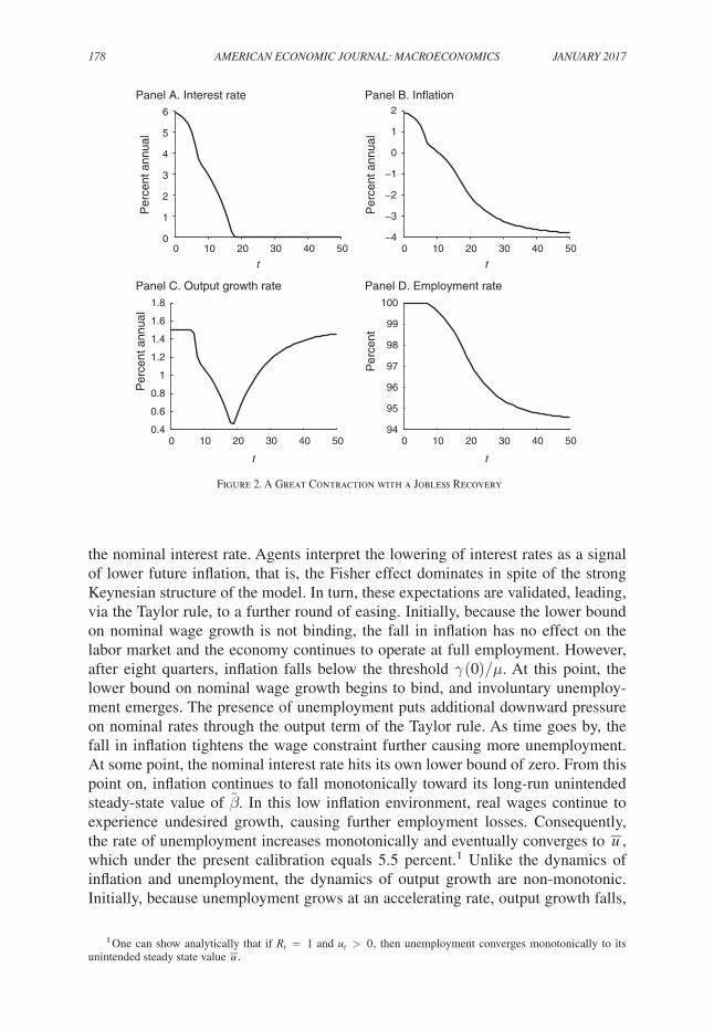
Figure 2 displays the equilibrium dynamics triggered by a period-0 revision in expectations that results in an initial inflation rate 10 annual basis points below the target rate π ∗ , that is π 0 = 1. 019 1/4 . We compute the exact nonlinear equilib-rium dynamics following the steps described in the proof of Proposition 5. Figure 2 shows that after the initial loss of confidence, inflation starts drifting down. As a response, the monetary authority, following the dictum of the Taylor rule, lowers


the nominal interest rate. Agents interpret the lowering of interest rates as a signal of lower future inflation, that is, the Fisher effect dominates in spite of the strong Keynesian structure of the model. In turn, these expectations are validated, leading, via the Taylor rule, to a further round of easing. Initially, because the lower bound on nominal wage growth is not binding, the fall in inflation has no effect on the labor market and the economy continues to operate at full employment. However, after eight quarters, inflation falls below the threshold γ (0)/μ . At this point, the lower bound on nominal wage growth begins to bind, and involuntary unemploy-ment emerges. The presence of unemployment puts additional downward pressure on nominal rates through the output term of the Taylor rule. As time goes by, the fall in inflation tightens the wage constraint further causing more unemployment. At some point, the nominal interest rate hits its own lower bound of zero. From this point on, inflation continues to fall monotonically toward its long-run unintended steady-state value of β . In this low inflation environment, real wages continue to experience undesired growth, causing further employment losses. Consequently, the rate of unemployment increases monotonically and eventually converges to _ u , which under the present calibration equals 5.5 percent.1 Unlike the dynamics of inflation and unemployment, the dynamics of output growth are non-monotonic. Initially, because unemployment grows at an accelerating rate, output growth falls,

1 One can show analytically that if r t = 1 and u t > 0 , then unemployment converges monotonically to its unintended steady state value _ u .

0 10 20 30 40 500.4

0.6

0.8

1

1.2

1.4

1.6

1.8

Panel C. Output growth rate

Per

cent

ann

ual

0 10 20 30 40 5094

95

96

97

98

99

100

Panel D. Employment rate

Per

cent

0 10 20 30 40 50−4

−3

−2

−1

0

1

2Panel B. Inflation

0 10 20 30 40 500

1

2

3

4

5

6

Panel A. Interest rate

Per

cent

ann

ual

Per

cent

ann

ual

t t

t t

Figure 2. A Great Contraction with a Jobless Recovery


reaching a trough in period 19, which coincides with the economy reaching the liquidity trap. As the rate of unemployment approaches its unintended steady-state level, output growth fully recovers to the rate of technological progress, μ , observed prior to the recession. However, this recovery is jobless, in the sense that unemploy-ment remains high, namely at 5.5 percent, the level consistent with the unintended steady state. To highlight the importance of non-fundamental loss of confidence shocks in generating jobless growth recoveries, we next analyze the dynamics trig-gered by fundamental shocks.

IV. Contractions with Job-Creating Recoveries

In this section, we characterize unemployment and inflation dynamics when inflationary expectations are well anchored. By well-anchored inflationary expec-tations, we mean environments in which agents expect inflation to converge toward its target level π ∗ . We show that when inflationary expectations are well anchored, a large negative fundamental demand shock, modeled as a decline in the natural rate of interest, causes deflation and unemployment on impact. More importantly, the key distinguishing characteristic of the adjustment when inflationary expectations are well anchored is that recoveries feature both output and employment growth. This is in sharp contrast to the dynamics triggered by a negative confidence shock, studied in Section III, which are characterized by a jobless growth recovery and the expectation that the economy will continue to be afflicted by low inflation and unemployment in the future.

As much of the recent related literature on liquidity traps (e.g., Eggertsson and Woodford 2003; Bilbiie, Monacelli, and Perotti 2014), we focus on disturbances to the natural rate of interest. As in the previous section, to preserve analytical trac-tability, we limit attention to perfect foresight equilibria. We first characterize the response of the model economy to purely temporary negative shocks to the natural real rate of interest and later consider the response to more persistent shocks. The natural rate of interest, defined as the real interest rate that would prevail in the absence of nominal rigidities, is given by β −1 e ξ t − ξ t+1 . A purely temporary negative natural rate shock is a situation in which at t = 0 , it is unexpectedly learned that ξ 0 − ξ 1 < 0 and that ξ t = ξ t+1 for all t ≥ 1 . Without loss of generality, we model a temporary decline in the natural rate of interest by setting ξ 0 < 0 and ξ t = 0 for all t ≥ 1 . The path of the natural rate of interest is then given by β −1 e ξ 0 < β −1 in period 0 , and β −1 for all t > 0 .

The following definition gives a precise meaning to the concept of perfect fore-sight equilibria with well-anchored inflationary expectations in the present context.

DEFINITION 1 (Equilibria with Well-Anchored Inflationary Expectations): suppose that ξ t is deterministic and that ξ t = 0 for all t ≥ T , for some T > 0 . Then, a perfect-foresight equilibrium with well-anchored inflationary expectations is a perfect-foresight equilibrium in which π t satisfies lim t→∞ π t = π ∗ .

The present model displays different responses to negative natural rate shocks depending on their magnitude. The interest-rate-feedback rule in place can preserve


full employment in response to small negative natural rate shocks by an appropriate easing of the nominal interest rate. But if the negative natural rate shock is large, the Taylor rule is unable to stabilize the economy and involuntary unemployment emerges.

The following proposition gives a lower bound for the set of natural rate shocks that can be fully neutralized, in the sense that they do not cause unemployment. We refer to natural rate shocks satisfying this bound as small. The proposition also shows that when inflationary expectations are well anchored, small negative natural rate shocks generate a temporary decline in inflation below its target level, π ∗ .

PROPOSITION 7 (Full Employment under Small Negative Natural Rate Shocks): suppose that Assumptions 1 and 2 hold, that w −1 = F ′ ( h ) , that

(19) 1 > e ξ 0 ≥ β _ π ∗ max {1, π ∗ _

β + α π ( γ (0)

_ μ − π ∗ ) } ,

and that ξ t = 0 for all t ≥ 1 . Then, there exists a unique perfect foresight equi-librium with well-anchored inflationary expectations. Furthermore, the equilibrium

features u t = 0 for all t ≥ 0 , γ(0 ) _ μ ≤ π 0 < π ∗ , and π t = π ∗ for all t > 0 .


The reason small negative shocks do not cause unemployment is that they can be fully accommodated by a downward adjustment in the nominal interest rate equal in size to the decline in the natural rate. Since the nominal interest rate cannot fall below zero, it follows immediately that one limit to accommodating negative shocks to the natural rate is the zero bound itself. But the present model delivers an addi-tional limit to the ability of a Taylor rule to stabilize natural rate shocks. Specifically, the model implies that inflation cannot fall below γ (0)/μ without causing unem-ployment. This threshold arises from the presence of downward nominal wage rigid-ity and may become binding before nominal interest rates hit the zero lower bound. If the inflation rate necessary to accommodate the exogenous decline in the natural rate is below γ (0)/μ , then the real wage will rise above its market clearing level causing involuntary unemployment.

The maximum natural rate shock that the monetary authority can fully offset by its interest rate policy depends on the characteristics of the interest rate feedback rule, especially the inflation coefficient α π and the inflation target π ∗ . If the mone-tary policy stance is aggressive, that is, if α π is sufficiently large, then the monetary authority can lower the nominal interest rate down to zero without pushing current inflation below γ (0)/μ , that is, without raising real wages in the current period. Under such monetary policy, the maximum natural rate shock the central bank can offset is one in which the natural rate is equal to the negative of the inflation target π ∗ . Hence, the larger is the inflation target, the larger is the range of negative shocks to the natural rate that the central bank can stabilize.


Consider now large negative shocks to the natural rate, that is, values of ξ 0 that violate condition (19). The following proposition shows that if the negative natural rate shock is large, the Taylor rule fails to preserve full employment.

PROPOSITION 8 (Unemployment Due to Large Negative Natural Rate Shocks): suppose that Assumptions 1 and 2 hold, that w −1 = F ′ ( h ) , that

(20) e ξ 0 < β _ π ∗ max {1, π ∗ _

β + α π ( γ (0)

_ μ − π ∗ ) } ,

and that ξ t = 0 for all t ≥ 1 . Then, in any perfect-foresight equilibrium with well-anchored inflationary expectations, the economy experiences unemployment in period 0, that is, u 0 > 0 .


To see why a large negative shock to the natural rate causes unemployment, it is of use to first understand how the optimal monetary policy (i.e., one that ensures full employment at all times) would react to such a shock. As in the case of small natural rate shocks, optimal policy calls for lowering the nominal interest rate in tan-dem with the decline in the natural rate. In this way, the real rate of interest can fall without igniting a future inflationary upward spiral. However, by the Taylor rule, the easing of current nominal rates must be accompanied by a fall in the current infla-tion rate. The latter in turn, if sufficiently large, drives up real wages in the current period, causing involuntary unemployment. A second impediment to preserving full employment in response to large negative shocks to the natural rate is the zero bound on nominal interest rates. This is because the required decline in the nominal interest rate that keeps the real interest rate equal to the natural rate without causing a rise in expected inflation may imply a negative nominal interest rate. If this is the case, then unemployment must necessarily emerge.

A central prediction of the present model is that when inflationary expectations are well anchored, the incidence of involuntary unemployment is transitory and that the recovery is accompanied by job creation. Specifically, after the shock, unemployment converges monotonically back to zero in finite time. In other words, the model predicts that jobless growth recoveries are impossible when inflationary expectations are well anchored. The following proposition formalizes this result.

PROPOSITION 9 (Recoveries with Job Creation): suppose that Assumptions 1 and 2 hold, that w −1 = F ′ ( h ) , that condition (20) holds, and that ξ t = 0 for all t ≥ 1 . Then, in any perfect-foresight equilibrium with well-anchored inflationary expec-tations, unemployment converges monotonically to zero in finite time. That is, 0 ≤ u t+1 ≤ u t for all t ≥ 0 , and there exists a date T > 0 , such that u T+j = 0 for all j ≥ 0 .



Furthermore, one can show that the nominal interest rate is either zero or close to zero in the period of the shock. However, the model does not predict the economy to remain in a liquidity trap during the recovery, that is, beyond period 0. In fact, already in period 1 the monetary authority raises the interest rate back to or above the

target level r ∗ (≡ π ∗ _ β ) . Similarly, inflation is at or above target starting in period 1.

If T = 1 , then not only employment but also inflation and the nominal interest rate return to the target steady state in period 1. If T > 1 , that is, when unemployment lasts longer than the shock itself, then interest rates and inflation are above target so that the economy is far from a liquidity trap during the recovery. Remarkably, in this case, tightening of policy occurs in an environment in which the economy has not yet fully recovered from the negative natural rate shock. During the transition, involuntary unemployment persists because the real wage is still above the level consistent with full employment. Because of downward nominal wage rigidity, the only way to reduce real wages quickly is to engineer temporarily higher price infla-tion. To this end, the central bank raises nominal rates to induce, through the Fisher effect, an elevation in the expected rate of inflation. The following proposition estab-lishes these results.

PROPOSITION 10 (Inflation and Interest Rate Dynamics Following a Large Temporary Natural Rate Shock): suppose that Assumptions 1 and 2 hold, that w −1 = F ′ ( h ) , that condition (20) holds, and that ξ t = 0 for all t ≥ 1 . Then, in any perfect-foresight equilibrium with well-anchored inflationary expectations, π 0 < π ∗ , π t > π ∗ for 0 < t < T , and π t = π ∗ for all t ≥ T , where T is defined in Propo-sition 9. Further, r 0 < r ∗ , r t > r ∗ for 0 < t < T , and r t = r ∗ for t ≥ T .

PROOF: See Appendix B.

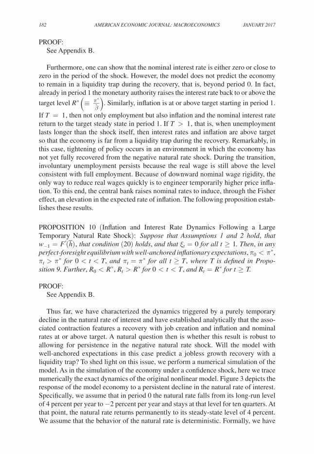
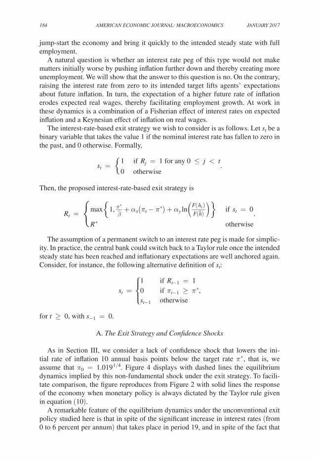
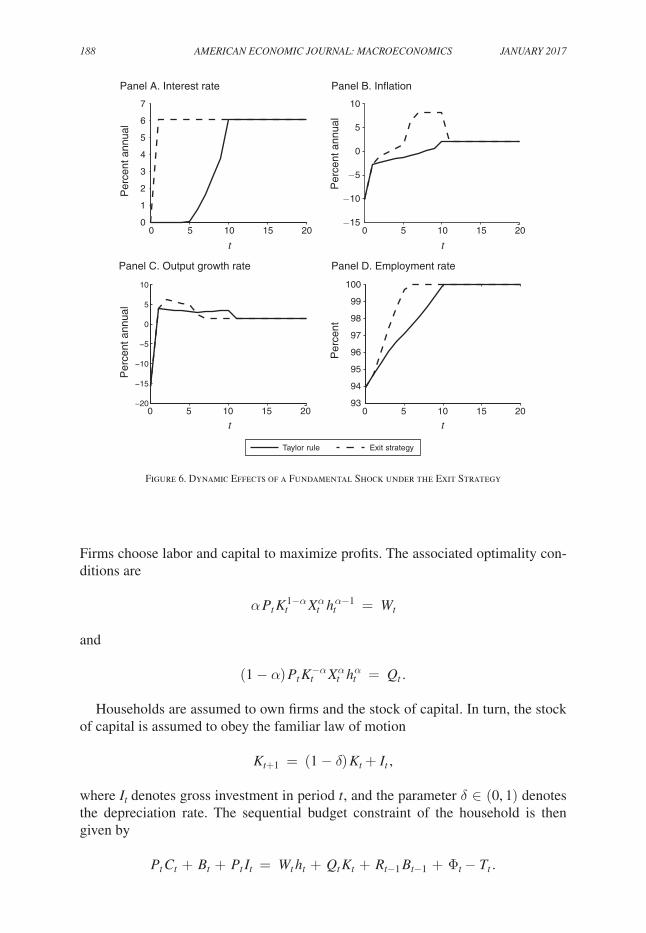
Thus far, we have characterized the dynamics triggered by a purely temporary decline in the natural rate of interest and have established analytically that the asso-ciated contraction features a recovery with job creation and inflation and nominal rates at or above target. A natural question then is whether this result is robust to allowing for persistence in the negative natural rate shock. Will the model with well-anchored expectations in this case predict a jobless growth recovery with a liquidity trap? To shed light on this issue, we perform a numerical simulation of the model. As in the simulation of the economy under a confidence shock, here we trace numerically the exact dynamics of the original nonlinear model. Figure 3 depicts the response of the model economy to a persistent decline in the natural rate of interest. Specifically, we assume that in period 0 the natural rate falls from its long-run level of 4 percent per year to −2 percent per year and stays at that level for ten quarters. At that point, the natural rate returns permanently to its steady-state level of 4 percent. We assume that the behavior of the natural rate is deterministic. Formally, we have


that ξ t − ξ t+1 = ln (0. 98 1/4 β ) for t = 0, … , 9 and ξ t − ξ t+1 = 0 for t ≥ 10 . We pick the size and duration of the natural rate shock following Eggertsson and Woodford (2003).2 All structural parameters of the model are as in the calibration presented in Section III.

The persistent natural rate shock produces an initial reduction in output growth, involuntary unemployment, deflation, and interest rates up against the zero bound. However, contrary to what happens under a confidence shock, the recovery from the negative natural rate shock features growth in both employment and output. That is, the recovery is characterized by job creation. Further, both output and employment begin to recover immediately after period zero. By contrast, the non-fundamental confidence shock generates a protracted slump.

V. Exiting the Slump: An Interest Rate Peg

In this section, we consider a monetary policy that succeeds in re-anchoring inflationary expectations when the economy finds itself in a liquidity trap with ele-vated unemployment due to lack of confidence. Specifically, we argue that an inter-est rate peg that raises the interest rate from zero to its intended target level can

2 These authors assume that the natural rate shock is stochastic and has an average duration of ten quarters and an absorbent state of 4 percent.

−15

−10

−5

0

5

Panel B. Inflation

Per

cent

ann

ual

93

94

95

96

97

98

99

100


Per

cent

0 5 10 15 200

1

2

3

4

5

6

7


Per

cent

ann

ual

t

0 5 10 15 20

t

0 5 10 15 20

t

0 5 10 15 20

t

−20

−15

−10

−5

0

5


Per

cent

ann

ual

Figure 3. A Contraction with a Job-Creating Recovery: Response to a Persistent Decline in the Natural Rate


jump-start the economy and bring it quickly to the intended steady state with full employment.

A natural question is whether an interest rate peg of this type would not make matters initially worse by pushing inflation further down and thereby creating more unemployment. We will show that the answer to this question is no. On the contrary, raising the interest rate from zero to its intended target lifts agents’ expectations about future inflation. In turn, the expectation of a higher future rate of inflation erodes expected real wages, thereby facilitating employment growth. At work in these dynamics is a combination of a Fisherian effect of interest rates on expected inflation and a Keynesian effect of inflation on real wages.

The interest-rate-based exit strategy we wish to consider is as follows. Let s t be a binary variable that takes the value 1 if the nominal interest rate has fallen to zero in the past, and 0 otherwise. Formally,

s t = { 1 if r j = 1 for any 0 ≤ j < t 0

otherwise .

Then, the proposed interest-rate-based exit strategy is

r t = {

max {1, π ∗ _ β + α π ( π t − π ∗ ) + α y ln ( F( h t ) _

F( h ) ) } if s t = 0

r ∗

otherwise

.

The assumption of a permanent switch to an interest rate peg is made for simplic-ity. In practice, the central bank could switch back to a Taylor rule once the intended steady state has been reached and inflationary expectations are well anchored again. Consider, for instance, the following alternative definition of s t :

s t = ⎧

⎪

⎨ ⎪

⎩ 1

if r t−1 = 1 0 if π t−1 ≥ π ∗

s t−1

otherwise ,

for t ≥ 0, with s −1 = 0 .

A. The Exit strategy and confidence shocks

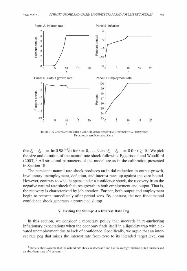
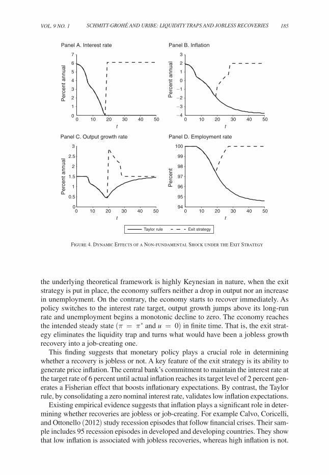
As in Section III, we consider a lack of confidence shock that lowers the ini-tial rate of inflation 10 annual basis points below the target rate π ∗ , that is, we assume that π 0 = 1. 019 1/4 . Figure 4 displays with dashed lines the equilibrium dynamics implied by this non-fundamental shock under the exit strategy. To facili-tate comparison, the figure reproduces from Figure 2 with solid lines the response of the economy when monetary policy is always dictated by the Taylor rule given in equation (10).

A remarkable feature of the equilibrium dynamics under the unconventional exit policy studied here is that in spite of the significant increase in interest rates (from 0 to 6 percent per annum) that takes place in period 19, and in spite of the fact that


the underlying theoretical framework is highly Keynesian in nature, when the exit strategy is put in place, the economy suffers neither a drop in output nor an increase in unemployment. On the contrary, the economy starts to recover immediately. As policy switches to the interest rate target, output growth jumps above its long-run rate and unemployment begins a monotonic decline to zero. The economy reaches the intended steady state ( π = π ∗ and u = 0 ) in finite time. That is, the exit strat-egy eliminates the liquidity trap and turns what would have been a jobless growth recovery into a job-creating one.

This finding suggests that monetary policy plays a crucial role in determining whether a recovery is jobless or not. A key feature of the exit strategy is its ability to generate price inflation. The central bank’s commitment to maintain the interest rate at the target rate of 6 percent until actual inflation reaches its target level of 2 percent gen-erates a Fisherian effect that boosts inflationary expectations. By contrast, the Taylor rule, by consolidating a zero nominal interest rate, validates low inflation expectations.

Existing empirical evidence suggests that inflation plays a significant role in deter-mining whether recoveries are jobless or job-creating. For example Calvo, Coricelli, and Ottonello (2012) study recession episodes that follow financial crises. Their sam-ple includes 95 recession episodes in developed and developing countries. They show that low inflation is associated with jobless recoveries, whereas high inflation is not.

0 10 20 30 40 50−4

−3

−2

−1

0

1

2

3

0 10 20 30 40 5094

95

96

97

98

99

100

0 10 20 30 40 500

1

2

3

4

5

6

7

0 10 20 30 40 500

0.5

1

1.5

2

2.5

3

Taylor rule

Panel B. Inflation




Per

cent

ann

ual

Per

cent

Per

cent

ann

ual

Per

cent

ann

ual

t

t

t

t

Exit strategy

Figure 4. Dynamic Effects of a Non-fundamental Shock under the Exit Strategy


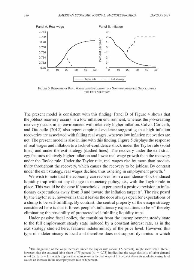
The present model is consistent with this finding. Panel B of Figure 4 shows that the jobless recovery occurs in a low inflation environment, whereas the job-creating recovery occurs in an environment with relatively higher inflation. Calvo, Coricelli, and Ottonello (2012) also report empirical evidence suggesting that high inflation recoveries are associated with falling real wages, whereas low inflation recoveries are not. The present model is also in line with this finding. Figure 5 displays the response of real wages and inflation to a lack-of-confidence shock under the Taylor rule (solid lines) and under the exit strategy (dashed lines). The recovery under the exit strat-egy features relatively higher inflation and lower real wage growth than the recovery under the Taylor rule. Under the Taylor rule, real wages rise by more than produc-tivity throughout the recovery, which causes the recovery to be jobless. By contrast under the exit strategy, real wages decline, thus ushering in employment growth.3

We wish to note that the economy can recover from a confidence-shock-induced liquidity trap without any change in monetary policy, i.e., with the Taylor rule in place. This would be the case if households’ experienced a positive revision in infla-tionary expectations away from β and toward the inflation target π ∗ . The risk posed by the Taylor rule, however, is that it leaves the door always open for expectations of a slump to be self-fulfilling. By contrast, the central property of the escape strategy considered here is that it forces people’s inflationary expectations to be π ∗ thereby eliminating the possibility of protracted self-fulfilling liquidity traps.

Under passive fiscal policy, the transition from the unemployment steady state to the full employment steady state induced by a constant interest rate, as in the exit strategy studied here, features indeterminacy of the price level. However, this type of indeterminacy is local and therefore does not support dynamics in which

3 The magnitude of the wage increases under the Taylor rule (about 1.5 percent), might seem small. Recall, however, that the assumed labor share of 75 percent ( α = 0.75 ) implies that the wage elasticity of labor demand is −4 (or 1/(α − 1) ), which implies that an increase in the real wage of 1.5 percent above its market-clearing level causes an increase in the unemployment rate of 6 percent.

0 10 20 30 40 500.75

0.752

0.754

0.756

0.758

0.76

0.762

0.764

Panel A. Real wage

0 10 20 30 40 50−4

−3

−2

−1

0

1

2

3

Panel B. Inflation

Per

cent

per

yea

r

Taylor rule Exit strategy

Figure 5. Response of Real Wages and Inflation to a Non-fundamental Shock under the Exit Strategy


the economy converges to the unemployment steady state. A coordinated switch of fiscal policy to an active stance would eliminate the local indeterminacy of the price level (Cochrane 2014).

B. The Exit strategy and Natural rate shocks

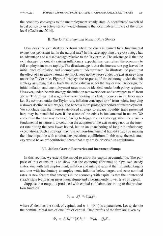
How does the exit strategy perform when the crisis is caused by a fundamental exogenous persistent fall in the natural rate? In this case, applying the exit strategy has an advantage and a disadvantage relative to the Taylor rule. The advantage is that the exit strategy, by quickly raising inflationary expectations, can return the economy to full employment more rapidly. The disadvantage is that the interest rate peg leaves the initial rates of inflation and unemployment indeterminate. To illustrate the point that the effect of a negative natural rate shock need not be worse under the exit strategy than under the Taylor rule, Figure 6 displays the response of the economy under the exit strategy assuming that π 0 takes the same value as under the Taylor rule. By design, the initial inflation and unemployment rates must be identical under both policy regimes. However, under the exit strategy, the inflation rate overshoots and converges to π ∗ from above. This brings real wages down contributing to a faster recovery in the labor mar-ket. By contrast, under the Taylor rule, inflation converges to π ∗ from below, implying a slower decline in real wages, and hence a more prolonged period of unemployment. We conclude that the interest-rate-based strategy to escape liquidity traps presented here may be beneficial even if the cause of the crisis is fundamental in nature. We conjecture that one way to avoid having to trigger the exit strategy when the crisis is fundamental in nature is to condition the adoption of the exit strategy not on the inter-est rate hitting the zero lower bound, but on an unanchoring of long-run inflationary expectations. Such a strategy may rule out non-fundamental liquidity traps by making them incompatible with a rational expectations equilibrium. In this case, the exit strat-egy would be an off-equilibrium threat that may not be observed in equilibrium.

VI. Jobless Growth Recoveries and Investment Slumps

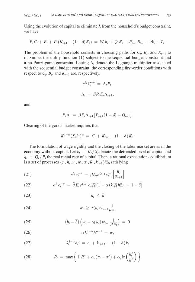
In this section, we extend the model to allow for capital accumulation. The pur-pose of this extension is to show that the economy continues to have two steady states, one with full employment, inflation and interest rates at their intended targets and one with involuntary unemployment, inflation below target, and zero nominal rates. A new feature that emerges in the economy with capital is that the unintended steady state features an investment slump and a permanently lower level of capital.

Suppose that output is produced with capital and labor, according to the produc-tion function

y t = K t 1−α ( X t h t ) α ,

where K t denotes the stock of capital, and α ∈ (0, 1) is a parameter. Let Q t denote the nominal rental rate of one unit of capital. Then profits of the firm are given by

Φ t = P t K t 1−α ( X t h t ) α − W t h t − Q t K t .


Firms choose labor and capital to maximize profits. The associated optimality con-ditions are

α P t K t 1−α X t α h t α−1 = W t

and

(1 − α) P t K t −α X t α h t α = Q t .

Households are assumed to own firms and the stock of capital. In turn, the stock of capital is assumed to obey the familiar law of motion

K t+1 = (1 − δ) K t + I t ,

where I t denotes gross investment in period t , and the parameter δ ∈ (0, 1) denotes the depreciation rate. The sequential budget constraint of the household is then given by

P t c t + B t + P t I t = W t h t + Q t K t + r t−1 B t−1 + Φ t − T t .

0 5 10 15 20−15

−10

−5

0

5

10

0 5 10 15 2093

94

95

96

97

98

99

100

0 5 10 15 200

1

2

3

4

5

6

7

0 5 10 15 20−20

−15

−10

−5

0

5

10

Panel B. Inflation

Per

cent

ann

ual


Per

cent


Per

cent

ann

ual


Per

cent

ann

ual

t

t

t

t


Figure 6. Dynamic Effects of a Fundamental Shock under the Exit Strategy


Using the evolution of capital to eliminate I t from the household’s budget constraint, we have

P t c t + B t + P t ( K t+1 − (1 − δ) K t ) = W t h t + Q t K t + r t−1 B t−1 + Φ t − T t .

The problem of the household consists in choosing paths for c t , B t , and K t+1 to maximize the utility function (1) subject to the sequential budget constraint and a no-Ponzi-game constraint. Letting Λ t denote the Lagrange multiplier associated with the sequential budget constraint, the corresponding first-order conditions with respect to c t , B t , and K t+1 are, respectively,

e ξ t c t −σ = Λ t P t ,

Λ t = β r t E t Λ t+1 ,

and

P t Λ t = β E t Λ t+1 [ P t+1 (1 − δ) + Q t+1 ].

Clearing of the goods market requires that

K t 1−α ( X t h t ) α = c t + K t+1 − (1 − δ ) K t .

The formulation of wage rigidity and the closing of the labor market are as in the economy without capital. Let k t ≡ K t / X t denote the detrended level of capital and q t ≡ Q t / P t the real rental rate of capital. Then, a rational expectations equilibrium is a set of processes { c t , h t , u t , w t , π t , r t , k t+1 } t=0 ∞ satisfying

(21) e ξ t c t −σ = β E t e ξ t+1 c t+1 −σ [ r t _ π t+1 ]

(22) e ξ t c t −σ = β E t e ξ t+1 c t+1 −σ [(1 − α) k t+1 −α h t+1 α + 1 − δ]

(23) h t ≤ h

(24) w t ≥ γ( u t ) w t−1 1 _ μ π t

(25) ( h t − h ) ( w t − γ( u t ) w t−1 1 _ μ π t ) = 0

(26) α k t 1−α h t α−1 = w t

(27) k t 1−α h t α = c t + k t+1 μ − (1 − δ ) k t

(28) r t = max {1, r ∗ + α π ( π t − π ∗ ) + α y ln ( h t α _

h α ) }


(29) u t = h − h t _ h .

Consider now steady-state equilibria. Suppose that ξ t = 0 for all t and that the set of sequences { c t , h t , u t , w t , π t , r t , k t+1 } t=0 ∞ is constant and equal to the vector { c, h, u, w, π, r, k} . Then, a steady-state equilibrium is given by

(30) π = β r

(31) 1 = β [(1 − α) k −α h α + 1 − δ]

(32) h ≤ h

(33) 1 ≥ γ(u ) 1 _ μπ

(34) (h − h ) (1 − γ(u ) w 1 _ μπ ) = 0

(35) α k 1−α h α−1 = w

(36) k 1−α h α = c + k [ μ − (1 − δ ) ]

(37) r = max {1, r ∗ + α π (π − π ∗ ) + α y ln ( h α _

h α ) }

(38) u = h − h _ h .

Steady-state conditions (30), (32)–(34), (37), and (38) are identical to the steady-state conditions of the economy without capital, and therefore admit two solutions, namely, (u, h, π, r) = (0, h , π ∗ , π ∗ / β ) and (u, h, π, r) = ( u , h L , β , 1) where, as before, u solves

γ( u ) = μ β .

It follows that Propositions 1 and 2 apply to the present economy with capital accumulation.

To obtain the steady-state levels of k , w , and c , note that steady-state condition (31) implies a unique steady-state value for the capital-labor ratio, denoted κ ,

κ ≡ k _ h = [ β −1 − 1 + δ _

1 − α ] −1/α

.

This implies the existence of two steady-state levels of the capital stock k ∗ ≡ κ h and k L ≡ κ h L . Thus, the unemployment steady state is characterized by a lower level of physical capital than in the intended steady state. Also, since the steady-state level of investment is proportional to the capital stock, we have that the unemployment


steady state also features a lower level of investment. From steady-state condition (35) we have that the steady-state real wage is unique and given by

w = α κ 1−α .

This result represents a difference from the economy without capital, where the steady-state real wage was higher in the liquidity trap than in the intended steady- state. Finally, equation (36) yields the following expression for the steady-state level of consumption:

c = [ κ 1−α − κ [ μ − (1 − δ ) ]] h,

which implies lower consumption in the liquidity trap than in the intended steady state.

A. A self-Fulfilling Investment slump

Here, we provide a constructive derivation of a self-fulfilling recession with a jobless growth recovery, an investment slump, low inflation, and zero nominal inter-est rates.

Consider the case of no fundamental shocks, that is, ξ t = 0 for all t ≥ 0 with probability one. Prior to period 0, the economy is assumed to have been at the intended steady state. Assume that in period 0, a confidence shock causes agents to expect that the economy will fall into a liquidity trap. Accordingly, let π 0 < π ∗ be given. Also given are the initial capital stock k 0 = k ∗ and the past real wage w −1 = α κ 1−α . Unlike the economy without capital, the presence of capital intro-duces the need to use a shooting-style algorithm to find the initial value of capital, k 1 , consistent with the economy converging to the liquidity trap. This feature of the construction of the equilibrium dynamics is typical of any rational expectations optimizing model with capital accumulation. Thus, the algorithm begins by guess-ing a value of k 1 and then tracing the perfect-foresight dynamics of the model. If the stock of capital fails to converge to the steady-state value k L , the guess of k 1 must be adjusted until convergence is achieved.

Given a guess for k 1 , the perfect-foresight equilibrium path is constructed as follows. For any t ≥ 0 , given the quadruplet { w t−1 , k t , k t+1 , π t } , the value of { w t , k t+1 , k t+2 , π t+1 } satisfying the equilibrium conditions (21)–(29) can be found as follows. Try h t = h and evaluate the labor demand (26). This yields a value for the real wage, w t . Now check if this value satisfies the wage lower bound (24). If so, then h t and w t have been determined. Otherwise, h t and w t are the solution to the system of two equations consisting of (24) holding with equality and (26). Use the Taylor rule (28) to obtain r t . Use the resource constraint (27) to obtain c t . Now guess that h t+1 = h . Then, the Euler equation for capital (22) can be solved for c t+1 and the Euler equation for bond holdings (21) for π t+1 . Solve (26) for w t+1 . Check whether this value satisfies the wage lower bound (24). If so, then π t+1 has been found. Otherwise, solve the system of four equations consisting of (21), (22), (24) holding with equality, and (26) for h t+1 , w t+1 , π t+1 , and c t+1 . This system can


be reduced to one equation in one unknown, h t+1 . In general, this equation does not admit a closed-form solution, but can be readily handled numerically. (In the special case of full depreciation, δ = 1 , a closed-form solution exists.) Finally, solve the resource constraint (27) for k t+2 . This completes the construction of the quadruplet { w t , k t+1 , k t+2 , π t+1 } , which serves as the initial condition for the next iteration. The result of this algorithm is a sequence for all endogenous variables that satisfies equi-librium conditions (21)–(29) as a function of k 1 . The equilibrium value of k 1 is the one that ensures that k t → k L .

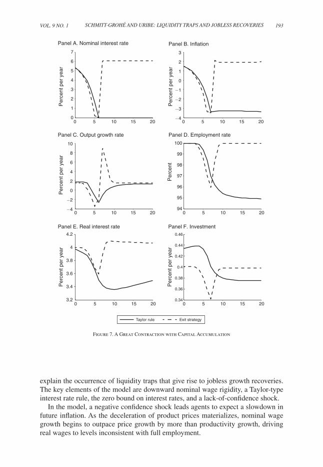
Figure 7 displays with solid lines the dynamics of the model with capital to a negative confidence shock that puts the economy in a downward path toward the liquidity trap. The parameter values used to construct the figure are the same as those used in Section III. In addition, the depreciation rate, δ , is set at 0.025. As in the economy without capital, the negative confidence shock causes a deceleration of price growth, a fall in the nominal interest rate, and a fall in employment and output growth. As the economy approaches the liquidity trap, output growth recovers, but the level of employment does not. Thus, the model with capital predicts a jobless growth recovery. Along the transition to the liquidity trap, the detrended level of investment falls and does not recover as long as the economy is trapped at the zero bound. Notably, the investment slump takes place in the context of low real interest rates. The reason why firms find it optimal to reduce investment is that the decline in employment reduces the rate of return of capital.

Figure 7 displays with broken lines the equilibrium dynamics under the exit strat-egy of raising the interest rate to the intended target r ∗ as soon as the economy hits the zero lower bound. This policy switch is successful at quickly raising inflationary expectations from below the target to the intended target of 2 percent per year. As a consequence, price growth begins to outpace wage growth, and the resulting erosion of real wages fosters employment.

In the absence of the exit strategy, the confidence shock results in a boom-bust cycle in investment, which ends in a chronic slump. The exit strategy eliminates both the initial boom and the chronic slump. Note that once the exit strategy is in place (i.e., once the interest rate is raised from 0 to its intended target of 6 percent per year), investment increases in spite of a rising real interest rate. The reason for this behavior is that along the recovery employment is growing, which causes, all other things equal, the marginal product of capital to rise incentivizing firms to invest in physical capital. We therefore have that, intuitively, the increase in the nominal interest rate that takes place as the exit strategy kicks in results in an increase in the real interest rate. However, the increase in the real interest rate is not associated with depressed investment. It follows that in the context of the present model, the stan-dard argument against raising interest rates, namely that it would make things worse by further weakening investment spending, does not apply.

VII. Conclusion

Jobless growth recoveries are situations in which after a contraction the rate of output growth returns to its pre-recession value while the level of output and employ-ment do not. The contribution of the present paper is to develop a model that can


explain the occurrence of liquidity traps that give rise to jobless growth recoveries. The key elements of the model are downward nominal wage rigidity, a Taylor-type interest rate rule, the zero bound on interest rates, and a lack-of-confidence shock.

In the model, a negative confidence shock leads agents to expect a slowdown in future inflation. As the deceleration of product prices materializes, nominal wage growth begins to outpace price growth by more than productivity growth, driving real wages to levels inconsistent with full employment.

0 5 10 15 200

1

2

3

4

5

6

7

Panel A. Nominal interest rate

Per

cent

per

yea

rP

erce

nt p

er y

ear

Per

cent

per

yea

r

Per

cent

per

yea

rP

erce

nt p

er y

ear

Per

cent

0 5 10 15 20−4

−3

−2

−1

0

1

2

3

Panel B. Inflation

0 5 10 15 20−4

−2

0

2

4

6

8

10


0 5 10 15 2094

95

96

97

98

99

100


0 5 10 15 203.2

3.4

3.6

3.8

4

4.2

Panel E. Real interest rate

0 5 10 15 200.34

0.36

0.38

0.4

0.42

0.44

0.46

Panel F. Investment


Figure 7. A Great Contraction with Capital Accumulation


The decline in employment along this transition causes a reduction in output growth. Eventually, the economy converges to an equilibrium featuring zero inter-est rates, low inflation, and persistent involuntary unemployment. In an environ-ment with capital accumulation, the economy experiences in addition an investment slump. However, due to secular technological progress, the growth rates of output, investment, and real wages return to their precrisis levels. Thus, the liquidity trap displays a jobless growth recovery.

Absent a change in policy or a revision of expectations, the state of matters described above becomes chronic. A successful policy intervention must spur inflation expectations, as a means to lower real wages to levels compatible with the restoration of full employment. The present paper proposes an interest-rate-based strategy for achieving this goal. It consists in pegging the nominal interest rate at its intended target level. The rationale for this strategy is the recognition that in a confidence-shock-induced liquidity trap, the effects of an increase in the nom-inal interest rate are quite different from what conventional wisdom would dic-tate. In particular, unlike what happens in normal times, in an expectations-driven liquidity trap, the nominal interest rate moves in tandem with expected infla-tion. Therefore, in the liquidity trap, an increase in the nominal interest rate is essentially a signal of higher future inflation. In turn, by its effect on real wages, future inflation stimulates employment, thereby lifting the economy out of the slump.

Appendix A: Data Sources

1. United States. Recession dates from the NBER.

2. United States. Real gross domestic product. Quarterly data, seasonally adjusted annual rates, GDP in billions of chained 2009 dollars. www.bea.gov/national/xls/gdplev.xls.

3. United States. Civilian noninstitutional population, 16 years and over, Labor Force Statistics from the Current Population Survey, BLS Series LNU00000000Q.

4. United States. Employment-population ratio, individuals age 16 years and over, BLS Data Series LNS12300000, Labor Force Statistics from the Current Population Survey, Seasonally Adjusted, quarterly average of monthly data.

5. United States. Effective Federal Funds Rate. Board of Governors of the Federal Reserve System. Table H.15 Selected Interest Rates. Quarterly aver-age of monthly data. Unique identifier H15/H15/RIFSPFF_N.M.

6. United States. GDP Deflator. Quarterly data, seasonally adjusted, year-over-year changes. www.bea.gov/national/xls/gdplev.xls.

www.bea.gov/national/xls/gdplev.xls


7. Japan. Recession dates. Economic and Social Research Institute (ESRI), Cabinet Office, Government of Japan, http://www.esri.cao.go.jp/en/stat/di/di2e.html.

8. Japan. Real GDP per capita and GDP deflator. SNA (National Accounts of Japan), Economic and Social Research Institute (ESRI), Cabinet Office, Government of Japan. http://www.esri.cao.go.jp/en/sna/data/sokuhou/files/2011/qe113/gdemenuea.html. The GDP deflator is at market prices and thus reflects consumption taxes. Following the BOJ Report “Price Developments in Japan, A Review Focusing on the 1990s,” Research and Statistics Department, Bank of Japan, October 6, 2000. Available online at http://www.boj.or.jp/en/research/brp/ron_2000/ron0010a.htm/, notes to Chart 6, we adjust the GDP deflator for the effects of the increase in the consumption tax in April 1997 from 3 to 5 percent by using a level-shift dummy.

9. Japan. Employed persons, labor force, not in labor force data is taken from the Labor Force Survey, Statistics Bureau, Ministry of Internal Affairs and Communications, http://www.stat.go/jp/english/data/roudou/lngindex.htm.

10. Japan. Call rate is taken from the Bank of Japan.

11. Europe. Recession dates are from CEPR.

12. Europe. Real GDP, dataset name: Eurostat ESA2010 TP, table 1; Frequency: quarterly; adjustment indicator: working day and seasonally adjusted; ref-erence area: euro area 19 (fixed composition); series name: MNA.Q.Y.I8.W2.S1.S1.B.B1GQ._Z._Z._Z.IX.LR.N; downloaded from ECB statistical warehouse.

13. Europe. Total Population. Euro area 19. Total population 15 to 64 years, quar-terly data, series name: lfsi_act_q. Downloaded from Eurostat.

14. Europe. Employment to population ratio, males. Source: Eurostat. Euro Area 19. Males, age 15 to 64. Quarterly data. Series name for male employment, lfsq_egan; series name for male population, lfsi_act_q.

15. Europe. Nominal Interest Rate. Eonia rate. Percent per year. Quarterly aver-age of monthly rate. Series ID: FM.M.U2.EUR.4F.MM.EONIA.HSTA. Downloaded from ECB statistical warehouse.

16. Europe. Inflation rate. Consumer price inflation. HICP–Overall index; Quarterly average of monthly observations, reference area: euro area, nei-ther seasonally nor working day adjusted, downloaded from Eurostat. Series name: ICP.M.U2.N.000000.4.ANR.

http://www.esri.cao.go.jp/en/stat/di/di2e.html

http://www.esri.cao.go.jp/en/sna/data/sokuhou/files/2011/qe113/gdemenuea.html

http://www.stat.go.jp/english/data/roudou/


Appendix B: Proofs of Propositions

PROOF OF PROPOSITION 1 (Existence and Uniqueness of the Full-Employment Steady State):

Set u = 0 . Then, h = h , c = F( h ) , and w = F ′ ( h ) are the unique solutions to (12), (13), and (17). Also, conditions (14) and (16) are satisfied. Combining (11) and (18), we have that π solves either

π _ β = π ∗ _

β + α π (π − π ∗ )

or

π _ β = 1.

By Assumption 2, the first expression admits a unique solution given by π = π ∗ . The second expression also admits a unique solution given by π = β . By equa-

tion (15), π must satisfy π ≥ γ (0) _ μ . According to assumptions 1 and 2, π = π ∗

satisfies this condition but π = β does not. When π = π ∗ , by Assumption 2, max {1, π ∗ / β + α π (π − π ∗ )} = π ∗ / β , which implies that π = π ∗ and r = π ∗ / β solve conditions (11) and (18). ∎

PROOF OF PROPOSITION 2 (Uniqueness of the Unemployment Steady State):Set u = u , where u > 0 is a constant to be determined. From (17), we have that

h < h . Combining (11) and (18), we have that the rate of inflation is determined by the solution to either

π _ β = π ∗ _

β + α π (π − π ∗ ) + α y ln ( F(h )

_ F( h )

)

or

π _ β = 1.

The solution to the first expression must satisfy π > π ∗ . This follows directly from

the assumption that α π β > 1 and the fact that α y ln ( F(h ) _

F( h ) ) is negative. But π > π ∗

cannot be the inflation rate at the unemployment steady state. To see this, note that by the slackness condition (16), condition (15) must hold with equality. That is, π = γ( u )/μ < γ(0)/μ < π ∗ . The last inequality follows from Assumption 2. Therefore, π cannot exceed π ∗ . This implies that if an unemployment steady state exists, it must be a liquidity trap, r = π / β = 1 . The unemployment rate in this steady state is determined by condition (15) holding with equality and evaluated at


π = β . That is, u is given by the solution to β = γ( u ) / μ . The fact that u > 0 fol-lows from the assumptions that β < γ(0) / μ and that γ is decreasing in u . Finally, it remains to show that equation (18) holds when π = β . That is, it remains to show

that max {1, π ∗ _ β + α π ( β − π ∗ ) + α y ln ( F(h )

_ F( h )

) } = 1 . To see this, note that

π ∗ _ β + α π ( β − π ∗ ) + α y ln ( F(h )

_ F( h )

) < π ∗ _ β + α π ( β − π ∗ )

= (

π ∗ _ β − 1

) (1 − α π β ) + 1

< 1.

This completes the proof. ∎

PROOF OF PROPOSITION 3 (Inflation Dynamics under Lack of Confidence):In any period t ≥ 0 , the economy can be in one of the following five situations:

(i) u t+1 = 0 and r t = 1 ; (ii) u t+1 = 0 and r t > 1 ; (iii) u t+1 > 0 and u t+1 ≥ u t ; (iv) u t > u t+1 > 0 and r t = 1 ; or (v) u t > u t+1 > 0 and r t > 1. The proof proceeds by establishing that for each of these situations, if the conditions of the proposition are satisfied, then π t+1 < π ∗ . Hence, in period t + 1 the conditions of the proposi-tion are again satisfied. This implies that π t+j < π ∗ for all j > 0 .

Situation (i), u t+1 = 0 and r t = 1 : because u t+1 = 0 , it follows from condi-tions (6) and (9) that h t+1 ≥ h t and by the assumed concavity of the utility function, we have that u ′ (F( h t+1 ))/ u ′ (F( h t )) ≤ 1 . Using (3) we have that π t+1 must satisfy π t+1 = β r t u ′ (F( h t+1 ))/ u ′ (F( h t )) ≤ β < γ (0)

_ μ < π ∗ , where the penultimate inequality follows from Assumption 1 and the last one from Assumption 2.

Situation (ii), u t+1 = 0 and r t > 1 : because r t > 1 , by (10), β r t − π t = ( α π β − 1)( π t − π ∗ ) − α y u t < 0 . By (3), it then follows that π t+1 = β r t u ′ (F( h t+1 ))/ u ′ (F( h t )) < π t u ′ (F( h t+1 ))/ u ′ (F( h t )) ≤ π t < π ∗ , where the penultimate inequality follows from the fact that h t+1 ≥ h t , and the last inequality follows from the assumption that π t < π ∗ .

Situation (iii), u t+1 > 0 and u t+1 ≥ u t : the assumptions of situation (iii) imply that h t+1 ≤ h t and by the concavity of the production function that F ′ ( h t )/ F ′ ( h t+1 ) ≤ 1 . Because u t+1 > 0 , condition (7) must hold with equality so

that π t+1 = γ( u t+1 ) _ μ F ′ ( h t ) _ F ′ ( h t+1 ) < γ(0 )

_ μ < π ∗ , where the last inequality is implied by Assumption 1.

Situation (iv), u t > u t+1 > 0 and r t = 1 : in this situation, h t < h t+1 , and hence

F( h t ) < F( h t+1 ) . This implies that u ′ (F( h t+1 )) _ u ′ (F( h t )) < 1 . From equilibrium condition (3)

we then have that π t+1 = β r t u ′ (F( h t+1 )) _ u ′ (F( h t ))

< β < γ(0 ) _ μ < π ∗ , where the penulti-

mate inequality follows from Assumption 1 and the last one from Assumption 2.


Situation (v), u t > u t+1 > 0 and r t > 1 : as in situation (iv), we have that h t <

h t+1 , and hence u ′ (F( h t+1 )) _ u ′ (F( h t )) < 1 . And as in situation (ii), we have r t > 1, and thus

(10) implies that β r t < π t . We then use (3) to obtain π t+1 = β r t u ′ (F( h t+1 )) _ u ′ (F( h t ))

< β r t < π t < π ∗ .

It remains to show that there exists a finite T such that π T < γ(0)/μ . Suppose that for some t ≥ 0 , u t = 0 and u t+1 > 0 . Then, (7) implies that

π t+1 = γ( u t+1 ) _ μ F ′ ( h ) _ F ′ ( h t+1 )

< γ( u t+1 ) _ μ < γ(0 ) _ μ . This shows the existence of a T such that

π T < γ (0)/ μ for the case of a switch from full employment to unemployment. Suppose now that u t = 0 for all t . Then, by (3), r t = π t+1 / β . Using this expres-sion to eliminate r t from (10) yields π t+1 = max { β , π ∗ + α π β ( π t − π ∗ )} . Because π t < π ∗ and because α π β > 1 , we have that π t reaches β < γ (0)/μ in finite time. This shows the existence of a T such that π T < γ (0)/μ . Finally, we must con-sider the case that u t > 0 for all t . In this case, we prove the existence of a period T such that π T < γ (0)/μ by contradiction. Suppose that π t ≥ γ (0)/μ for all t . We have already shown that under the assumptions of the proposition π t+1 < max { π t , γ(0)/μ} . This means that as long as π t ≥ γ(0)/μ , π t must be mono-tonically decreasing over time. Since, by assumption π t is bounded below by γ (0)/μ , we have that π t must converge. Let lim t→∞ π t ≡ π _ ≥ γ(0)/ μ . Since, by assumption, u t > 0 for all t , (7) must hold with equality at all times, that is, π t = γ( u t ) _ μ F ′ ( h t−1 ) _ F ′ ( h t )

. Because π t ≥ γ(0)/μ > γ ( u t ) / μ , we have that F ′ ( h t−1 ) > F ′ ( h t ) . This means, by the fact that u t = ( h − h t )/ h and by the concavity of F , that u t is decreasing in t . Since u t is bounded below by 0, we have that u t must converge. Let u _ ≡ lim t→∞ u t . Clearly, 0 ≤ u _ < 1. The fact that u _ < 1 implies that lim t→∞ F ′ ( h t ) exists and is finite. Taking limits of (7) we obtain

π _ = lim t→∞ γ( u t ) _ μ F ′ ( h t−1 ) _ F ′ ( h t ) = γ( u _ ) ___ μ lim t→∞ F ′ ( h t−1 ) _ F ′ ( h t )

= γ ( u _ ) ___ μ . Since π _ ≥ γ(0)/μ and

since γ ( · ) is strictly decreasing in u t , we have that u _ = 0 . Using (10), we have that lim t→∞ β r t = max { β , π ∗ + α π β ( π _ − π ∗ )} . Now by (3), we have that

β lim t→∞ r t = π _ lim t→∞ u ′ (F( h t ) ) _ u ′ (F( h t+1 ) ) = π _ . Combining these two expressions, we

obtain π _ = max { β , π ∗ + α π β ( π _ − π ∗ )} . This expression has two solutions for π _ , namely, β and π ∗ . Because β < γ(0)/μ and because we have already shown that π t < π ∗ for all t , both of these solutions yield a contradiction. ∎

PROOF OF PROPOSITION 4 (Chronic Involuntary Unemployment under Lack of Confidence):

The proof is by contradiction. Suppose that for some t ≥ T , u t = 0 . Then,

by condition (7), π t ≥ γ(0 ) _ μ F ′ ( h t−1 ) _

F ′ ( h ) ≥ γ(0 )

_ μ . This is a contradiction, because, by

Proposition 3, π t < γ (0)/μ . ∎


PROOF OF PROPOSITION 5 (Existence and Uniqueness of Chronic Unemployment Equilibria):

Consider the equilibrium conditions (3)–(10). Set ξ t = 0 for all t . Use (4) to eliminate c t from (3), and (5) to eliminate w t from (8) and (7). Then the set of perfect-foresight equilibrium conditions involves only deterministic sequences for { π t+1 , h t , u t , r t } t=0 ∞ given π 0 and h −1 = h . The proof is by construction. Suppose first that the initial value for π 0 satisfies γ (0)/μ ≤ π 0 < π ∗ . First, we show that in this case u 0 = 0 . Suppose the contrary, that is, u 0 > 0 . Then, by (9), h 0 < h , and

by (7), π 0 = γ( u 0 ) _ μ F ′ ( h ) _ F ′ ( h 0 ) < γ ( u 0 ) _ μ < γ (0 )

_ μ , where the penultimate inequality fol-

lows from the concavity of the function F( · ) and from h 0 < h , and the last inequal-ity follows from Assumption 1. But this is a contradiction. It follows that u 0 = 0 and h 0 = h . Then r 0 is uniquely determined by (10). We have therefore shown that there are unique values for h 0 , u 0 , and r 0 if γ (0)/μ ≤ π 0 < π ∗ .

To find π 1 , proceed as follows. Note that by (3), π 1 = β r 0 u ′ (F( h 1 )) _ u ′ (F( h ))

≥ β r 0 . Now

distinguish two cases: (i) β r 0 ≥ γ (0)/μ and (ii) β r 0 < γ (0)/μ . In case (i), we have π 1 ≥ γ (0)/μ . And as we just have shown if in any period t we have h t−1 = h and π t ≥ γ(0)/μ , then the period t perfect foresight solution is unique and fea-tures u t = 0 . In case (ii), β r 0 < γ (0)/μ . To rule out u 1 = 0 , note that if u 1 were 0, then by (3), π 1 = β r 0 < γ (0)/μ . At the same time, by (7), π 1 ≥ γ(0)/μ . This results in a contradiction, and it follows if a perfect foresight equilibrium exists, it must feature u 1 > 0 . Next, we show that in this case there exists a unique u 1 > 0 .

Combining (3) and (7) holding with equality yields γ( u 1 ) _ μ = β r 0 u ′ (F( h 1 )) F ′ ( h 1 ) _ u ′ (F( h 0 )) F ′ ( h 0 )

.

Notice that the left-hand side of this expression is monotonically decreasing in u 1 and that at u 1 = 0 , it takes the value γ (0)/μ . The right-hand side is monotonically increasing in u 1 , and at u 1 = 0 it takes the value β r 0 < γ (0)/μ . Hence, at u 1 = 0 the left-hand side exceeds the right-hand side. Further, as u 1 approaches 1, the right-hand side approaches infinity, so that as u 1 approaches 1, the left-hand side is smaller than the right-hand side. It follows that there is a single crossing, and there-fore there exists a single value u 1 that solves this expression. Given u 1 , use (9) to find h 1 , (3) to find π 1 , and use (10) to find r 1 . This shows that also in case (ii), there exist unique values for π 1 , r 0 , u 0 , h 0 that satisfy conditions (3)–(10), given γ (0)/μ ≤ π 0 < π ∗ and h −1 = h .

To find values for π t+1 , r t , u t , h t given h t−1 , and π t for t ≥ 1 , note that if h t−1 = h and if γ (0)/μ ≤ π t < π ∗ , then we can use the same arguments as those used above to construct the perfect foresight equilibrium for period t . It follows that for t = 1 , because we have already shown that h 0 = h and u 0 = 0 , we only need to check whether π 1 ≥ γ (0)/μ . If so, then we can proceed with the construction of the equi-librium as above, that is, we obtain u 1 = 0 , h 1 = h , and r 1 and π 2 in the same fashion as described above.

If however, π t < γ (0)/μ , construct the perfect-foresight equilibrium as follows. By Proposition 4, in this case u t > 0 . Given π t , use (7) holding with equality to find a unique value for u t . To see that this condition has a unique solution write it as: π t F ′ ( h t )/ F ′ ( h t−1 ) = γ ( u t ) / μ . The left-hand side is increasing in u t and converges


to infinity as u t approaches unity. At u t = 0 , it is less than or equal to π t , and hence less than γ (0) /μ . The right-hand side is monotonically decreasing. At u t = 0, it is equal to γ (0)/μ . Thus, at u t = 0 the left-hand side is smaller than the right-hand side. Consequently, we must have a single crossing implying a unique value for u t . With u t in hand and π t given, use (10) to find r t . From Proposition 3, we have that π t+1 < γ(0)/μ , and from Proposition 4, we have that u t+1 > 0 . Combine (3) and (7) holding with equality to obtain γ( u t+1 ) _ μ = β r t

u ′ (F( h t+1 ) ) F ′ ( h t+1 ) ___________ u ′ (F( h t ) ) F ′ ( h t ) . Use this

expression to find u t+1 . The left-hand side of this expression is decreasing and at u t+1 = 0 equal to γ (0)/μ . The right-hand side is monotonically increasing in u t+1 . At u t+1 = u t > 0, it is equal to β r t . Notice that β r t ≤ max { β , π t } < γ (0)/μ . Therefore, at u t+1 = 0 , the right-hand side must be less than the left-hand side. As u t+1 approaches unity, the right-hand side becomes infinity. Therefore, there exists a single crossing. This shows that u t+1 is unique. With u t+1 in hand, use (3) to find π t+1 . We have therefore shown how to construct values for u t , h t , r t , π t+1 in the case that π t < γ (0)/μ for an arbitrary h t−1 and that the so constructed values are unique. We can proceed in this fashion to obtain { h t , u t , r t , π t+1 } t=0 ∞ . ∎

PROOF OF PROPOSITION 6 (Convergence to a Liquidity Trap with Unemployment):

By Proposition 3, inflation is always strictly below its target level π ∗ . This means that the economy cannot converge to the full-employment steady state (π, r, u ) = ( π ∗ , r ∗ , 0) . Since the only remaining steady state is the unemployment steady state, the claim of the proposition must hold. ∎

PROOF OF PROPOSITION 7 (Full Employment under Small Negative Taste Shocks):

First, we show that if condition (19) is satisfied, then an equilibrium with u t = 0 for all t ≥ 0 , π 0 < π ∗ , and π t = π ∗ for t > 0 exists. The proof proceeds by showing that the proposed equilibrium path satisfies the complete set of equilib-rium conditions, given by expressions (3)–(10) for all t ≥ 0 . Setting h t = h for all t ≥ 0 ensures that (6), (8), and (9) hold for all t . Then, setting c t = F( h ) for all t ≥ 0 and w t = F ′ ( h ) ensures the satisfaction of (4) and (5) for all t ≥ 0 . Setting r 0 = e ξ 0 π ∗ _

β and r t = π ∗ _

β for all t > 0 implies that (3) holds for all t ≥ 0 .

Condition (19) guarantees that r 0 ≥ 1 . To ensure that (10) holds in period 0 , set π 0 at a value satisfying e ξ 0 π ∗ / β ≥ π ∗ / β + α π ( π 0 − π ∗ ) . That is, pick π 0 such that

π 0 ≤ π ∗ + ( e ξ 0 − 1) π ∗ _ β α π

. Clearly, π 0 < π ∗ . At the same time, for (7) to be satisfied

at t = 0 , π 0 must take values in the range π 0 ≥ γ(0)/ μ . Combining the above two

inequalities, we obtain that π ∗ + ( e ξ 0 − 1) π ∗ _ β α π

≥ π 0 ≥ γ(0)/μ . Condition (19) guarantees that this interval is nonempty. Finally, Assumption 2 guarantees that the proposed equilibrium satisfies (7) and (10) for all t > 0 . This completes the proof of existence of an equilibrium with well-anchored inflationary expectations.

The proof of uniqueness proceeds by first establishing that any equilibrium with well-anchored expectations must feature π t ≥ π ∗ for any t > 0 . This result is a


direct implication of Proposition 3, which shows that if for any t > 0 , π t < π ∗ , then π t+j < π ∗ for all j > 0 . By definition, an equilibrium with such a path for inflation is not one with well-anchored inflationary expectations. The next step is to show that under the conditions given in the proposition u 0 = 0 . This result is implied by Lemma 1 in Appendix C. It also follows that h 0 = h and that w 0 = F ′ ( h ) . Then Lemmas 2 and 3 in Appendix C show that in any equilib-rium with well-anchored inflationary expectations u t = 0 for all t > 0 and that π t = π ∗ for all t > 0 , respectively. It remains to be shown that π 0 is unique. Evaluating (3) at t = 0 yields a unique value of r 0 , given by r 0 = e ξ 0 π ∗ / β . Since the event e ξ 0 π ∗ / β = 1 is of measure zero, we have, by condition (19), that r 0 > 1 in general. Then we use this expression to eliminate r 0 from (10) to obtain e ξ 0 π ∗ / β = π ∗ / β + α π ( π 0 − π ∗ ) , which uniquely determines π 0 .4 ∎

PROOF OF PROPOSITION 8 (Unemployment Due to Large Negative Taste Shocks):

The proposition follows directly from Lemmas 3 and 4 in Appendix C. Lemma 4 establishes that if u 0 = 0 , then π 1 must be greater than π ∗ . Lemma 3 establishes that no equilibrium with well-anchored inflationary expectations exists if u 0 = 0 and π 1 > π ∗ ∎.

PROOF OF PROPOSITION 9 (Recoveries with Job Creation):We first show that u t+1 ≤ u t for all t ≥ 0 . If u t+1 = 0 , then this condition is

satisfied. If u t+1 > 0 , then (7) states that π t+1 = γ( u t+1 ) _ μ F ′ ( h t ) _ F ′ ( h t+1 ) < π ∗ F ′ ( h t ) _ F ′ ( h t+1 )

. Because, Proposition 3, π t+1 ≥ π ∗ , the above expression implies that h t+1 > h t or that u t+1 < u t . To show that unemployment disappears in finite time, note that

if u t+1 > 0 , then the above analysis yields F ′ ( h t ) _ F ′ ( h t+1 ) ≥ π ∗ _

( γ( u t+1 ) _ μ ) . Since γ( u t+1 ) _ μ is

bounded above by γ(0 ) _ μ < π ∗ , we have that F ′ ( h t ) _ F ′ ( h t+1 )

is bounded below by the con-

stant π ∗ _ ( γ(0 )

_ μ ) > 1 . This means that u t+1 − u t is negative and bounded away from

zero. Thus, u t+1 must reach zero in finite time. ∎

PROOF OF PROPOSITION 10 (Inflation and Interest Rate Dynamics):It follows directly from Proposition 3 that π t ≥ π ∗ for t > 0 in any equilib-

rium with well-anchored inflationary expectations and under the assumptions of the proposition. To see that π 0 < π ∗ notice that because, by Proposition 8, u 0 > 0 , condition (7) must hold with equality in period 0, that is,

π 0 = γ( u 0 ) _ μ F ′ ( h ) _ F ′ ( h 0 ) < γ( u 0 ) _ μ < γ(0 )

_ μ < π ∗ . The first inequality follows from

the fact that h 0 < h and the concavity of F ; the second inequality follows from Assumption 1; the third follows from Assumption 2. Because u 0 > 0 and

4 Even in the event that e ξ 0 π ∗ / β = 1 , this last expression would uniquely determine π 0 provided the parameter

configuration is such that π ∗ _ β + α π ( γ(0 )

_ μ − π ∗ ) ≥ 1 .


π 0 < π ∗ , equation (10) implies that r 0 < π ∗ / β ≡ r ∗ . The result that π t ≥ π ∗ for t > 0 together with Lemma 4 in Appendix C implies that π t = π ∗ for all t > T . To see that π T = π ∗ , note that, by condition (3) and the facts that u T = u T+1 = 0 and that π T+1 = π ∗ , r T = π ∗ / β > 1 . Using this expression to eliminate r T from (10) and taking into account that u T = 0 , yields π T = π ∗ . It remains to establish that π t > π ∗ for 0 < t < T . By (3), we have that for

0 < t < T , r t = π t+1 _ β u ′ (F( h t ) ) _ u ′ (F( h t+1 ) )

> π t+1 _ β ≥ π ∗ _

β > 1 . The first inequality follows

from the result that h t+1 > h t established in Proposition 9. The second inequality follows from the result that π t ≥ π ∗ . Using this expression to eliminate r t from (10) and taking into account that u t is positive for 0 < t < T , we obtain π t > π ∗ for 0 < t < T . ∎

Appendix C: Lemmas

LEMMA 1: suppose that Assumptions 1 and 2 hold, that w −1 = F ′ ( h ) , that con-dition (19) holds, and that ξ 1 = 0 with probability 1. Then u 0 > 0 implies that π 1 < π ∗ .

PROOF:If u 0 > 0 , then h 0 < h and (7) must hold with equality, so that π 0 is given

by π 0 = γ( u 0 ) _ μ F ′ ( h ) _ F ′ ( h 0 ) < γ(0 )

_ μ . Use (10) to obtain that the nominal interest rate in

period 0 is given by r 0 = max {1, π ∗ _ β + α π ( γ( u 0 ) _ μ F ′ ( h )

_ F ′ ( h 0 ) − π ∗ ) − α γ u 0 } . Consider

first the case that r 0 > 1 . It follows that 1 < r 0 < π ∗ _ β + α π ( γ(0 )

_ μ − π ∗ ) . This

expression together with condition (19) implies that e ξ 0 > β _ π ∗ r 0 . Solve (3) for e ξ 0

to obtain e ξ 0 = β r 0 u ′ ( c 1 ) _ u ′ ( c 0 ) π 1

. Combining this expression with the above inequality

yields β r 0 u ′ ( c 1 ) _ u ′ ( c 0 ) π 1

> β _ π ∗ r 0 . Rearrange to obtain u ′ ( c 1 ) _ u ′ ( c 0 ) > π 1 _ π ∗ . Suppose, contrary

to the claim of the lemma, that π 1 ≥ π ∗ . This and the previous inequality imply that u ′ ( c 1 ) > u ′ ( c 0 ) , or equivalently, that c 1 < c 0 . In turn, c 1 < c 0 implies that u 1 > u 0 > 0 and that h 1 < h 0 . Hence, in period 1, (7) must hold with equality and π 1 = γ( u 1 ) _ μ F ′ ( h 0 ) _ F ′ ( h 1 )

< γ( u 1 ) _ μ < γ(0 ) _ μ < π ∗ , which is a contradiction. We have there-

fore established that the statement of the lemma holds in the case in which r 0 > 1 .

Suppose now that r 0 = 1 . Then, one can rewrite equation (3) as e ξ 0 π ∗ _ β π 1 _ π ∗ = u ′ (F( h 1 )) _ F ′ ( h 0 )

.

Suppose that, contrary to the statement of the lemma, π 1 ≥ π ∗ . Then, by, condi-tion (19), the left-hand side of the above expression must be greater than or equal

to unity. This implies that so must be the right-hand side, that is, u ′ (F( h 1 )) _ F ′ ( h 0 ) ≥ 1 , or

h 1 ≤ h 0 . This means that u 1 ≥ u 0 > 0 . This means that (7) must hold with

equality in period 1. That is, π 1 = γ( u 1 ) _ μ F ′ ( h 0 ) _ F ′ ( h 1 ) ≤ γ( u 1 ) _ μ < γ(0 )

_ μ < π ∗ . But this


is a contradiction. Therefore, it must be the case that π 1 < π ∗ as claimed by the lemma. ∎

LEMMA 2: suppose Assumptions 1 and 2 hold and w t−1 = F ′ ( h ) . Assume further that ξ t = 0 for all t with probability 1. Then, any equilibrium in which π t ≥ π ∗ must feature u t = 0 .

PROOF:The proof is by contradiction. Suppose π t ≥ π ∗ and u t > 0 . Then, by (9) h t < h .

Equations (8) and (7) together then imply that π t = γ( u t ) _ μ F ′ ( h ) _ F ′ ( h t ) < γ(0 )

_ μ < π ∗ , which contradicts the maintained assumption that π t ≥ π ∗ . The first inequality fol-lows from the assumption that F( · ) is strictly concave and from Assumption 1, and the second inequality follows from Assumption 2. ∎

LEMMA 3: suppose Assumptions 1 and 2 hold and w t−1 = F ′ ( h ) . Assume further that ξ t = 0 for all t with probability 1. Then, any equilibrium in which π t > π ∗ features lim j→∞ π t+j = ∞ .

PROOF:Suppose π t > π ∗ . Given the conditions stated in the current lemma, it fol-

lows from Lemma 2 that u t = 0 . Condition (10) then yields that r t = π ∗ _ β +

α π ( π t − π ∗ ) > π ∗ _ β > 1 . Solve (3) for π t+1 to obtain π t+1 = β r t

u ′ (F( h t+1 ) ) _ u ′ (F( h ) )

. Because u( · ) and F( · ) are concave and because, by (6), h t+1 ≤ h , we have that π t+1 ≥ β r t . Use the above expression to eliminate r t . This yields: ( π t+1 − π ∗ ) ≥ β α π ( π t − π ∗ ) . Because, by Assumption 2, β α π > 1 , we have that π t+1 > π t . Since w t = F ′ ( h ) and π t+1 > π ∗ , the conditions of the lemma are also sat-isfied for period t + 1 , which means that by the above arguments π t+2 − π ∗ ≥ β α π ( π t+1 − π ∗ ) . Continuing with this argument yields that lim j→∞ π t+j = ∞ . ∎

LEMMA 4: If the taste shock is such that condition (19) is not satisfied and Assumptions 1 and 2 hold and w −1 = F ′ ( h ) , any equilibrium featuring u 0 = 0 must also feature π 1 > π ∗ .

PROOF:The proof is in two steps, one corresponding to the case in which condition (19)

is violated because its left-hand side is less than the first argument on the right-hand side, and the other corresponding to the case in which the left-hand side is less than the second argument on the right-hand side.

Step 1: Suppose e ξ 0 < β / π ∗ . Then, (3) implies that r 0 = u ′ (F( h )) _ u ′ (F( h 1 )) e

ξ 0 π ∗ _ β π 1 _ π ∗ .

Because u ′ (F( h ) ) _ u ′ (F( h 1 ) ) ≤ 1 , e

ξ 0 π ∗ _ β < 1 , and r 0 ≥ 1 , we have that π 1 > π ∗ as claimed

by the lemma.


Step 2: Suppose e ξ 0 < γ(0) α π β _ μ π ∗ + 1 − α π β . By (3), r 0 = u ′ (F( h )) _ u ′ (F( h 1 )) e

ξ 0 π ∗ _ β π 1 _ π ∗ . From

(10), r 0 ≥ π ∗ _ β + α π ( π 0 − π ∗ ) . Combine these two expressions and solve for π 0 to

obtain π 0 ≤ [ u ′ (F( h )) _ u ′ (F( h 1 )) e

ξ 0 π ∗ _ β π 1 _ π ∗ − π ∗ _

β ] α π −1 + π ∗ . From (7), π 0 ≥ γ(0)

_ μ . Combining

these two inequalities, we obtain u ′ (F( h )) _ u ′ (F( h 1 )) e

ξ 0 π 1 _ π ∗ ≥ γ(0) _ μ α π β _ π ∗ > e ξ 0 . The last inequal-

ity follows from the assumption that the left-hand side of (19) is less than the second argument of its right-hand side. The above condition implies that π 1 > π ∗ . ∎

REFERENCES

Aruoba, S. Boragan, Pablo Cuba-Borda, and Frank Schorfheide. 2014. “Macroeconomic Dynam-ics Near the ZLB: A Tale of Two Countries.” http://www.cepr.org/sites/default/files/events/1835_SCHORFHEIDE%20-%20Macroeconomic%20Dynamics%20Near%20the%20ZLB.pdf.

Barattieri, Alessandro, Susanto Basu, and Peter Gottschalk. 2014. “Some Evidence on the Importance of Sticky Wages.” American Economic Journal: Macroeconomics 6 (1): 70–101.

Benhabib, Jess, Stephanie Schmitt-Grohé, and Martín Uribe. 2001. “The Perils of Taylor Rules.” Jour-nal of Economic Theory 96 (1–2): 40–69.

Benigno, Gianluca, and Luca Fornaro. 2015. “Stagnation Traps.” https://www.imf.org/external/np/seminars/eng/2015/secularstag/pdf/Benigno.pdf.

Bilbiie, Florin O., Tommaso Monacelli, Roberto Perotti. 2014. “Is Government Spending at the Zero Lower Bound Desirable?” National Bureau of Economic Research (NBER) Working Paper 20687.

Calvo, Guillermo A., Fabrizio Coricelli, and Pablo Ottonello. 2012. “Labor Market, Financial Crises and Inflation: Jobless and Wageless Recoveries.” National Bureau of Economic Research (NBER) Working Paper 18480.

Cochrane, John H. 2014. “Monetary Policy with Interest on Reserves.” https://faculty.chicagobooth.edu/john.cochrane/research/papers/cochrane_policy.pdf.

Daly, Mary, Bart Hobijn, and Brian Lucking. 2012. “Why Has Wage Growth Stayed Strong?” FrBsF Economic Letter, April 2. http://www.frbsf.org/economic-research/publications/economic-letter/2012/april/strong-wage-growth/.

Eggertsson, Gauti B., and Neil R. Mehrotra. 2014. “A Model of Secular Stagnation.” National Bureau of Economic Research (NBER) Working Paper 20574.

Eggertsson, Gauti B., and Michael Woodford. 2003. “The Zero Bound on Interest Rates and Optimal Monetary Policy.” Brookings Papers on Economic Activity 33 (1): 139–211.

Gottschalk, Peter. 2005. “Downward Nominal-Wage Flexibility: Real or Measurement Error?” review of Economics and statistics 87 (3): 556–68.

Holden, Steinar, and Fredrik Wulfsberg. 2008. “Downward Nominal Wage Rigidity in the OECD.” B. E. Journal of Macroeconomics 8 (1): Article 30.

Krugman, Paul R. 1998. “Its Baaack! Japan’s Slump and the Return of the Liquidity Trap.” Brookings Papers on Economic Activity 28 (2): 137–205.

Kuroda, Sachiko, and Isamu Yamamoto. 2003. “Are Japanese Nominal Wages Downwardly Rigid? (Part I): Examinations of Nominal Wage Change Distributions.” Monetary and Economic studies 21 (2): 1–29.

Mertens, Karel R. S. M., and Morten O. Ravn. 2014. “Fiscal Policy in an Expectations Driven Liquid-ity Trap.” review of Economic studies 81 (4): 1637–67.

Schmitt-Grohé, Stephanie, and Martín Uribe. 2016. “Downward Nominal Wage Rigidity, Currency Pegs, and Involuntary Unemployment.” Journal of Political Economy 124 (5): 1466–1514.

Schmitt-Grohé, Stephanie, and Martín Uribe. 2017. “Liquidity Traps and Jobless Recoveries: Data-set.” American Economic Journal: Macroeconomics. https://doi.org/10.1257/mac.20150220.

Shimer, Robert. 2012. “Wage rigidity and jobless recoveries.” Journal of Monetary Economics 59 (Supplement): S65–77.

Taylor, John B. 1993. “Discretion versus policy rules in practice.” carnegie-rochester conference series on Public Policy 39: 195–214.

Woodford, Michael. 2012. “Methods of Policy Accommodation at the Interest-Rate Lower Bound.” https://www.kansascityfed.org/publicat/sympos/2012/mw.pdf.

http://www.cepr.org/sites/default/files/events/1835_SCHORFHEIDE%20-%20Macroeconomic%20Dynamics%20Near%20the%20ZLB.pdf

https://www.imf.org/external/np/seminars/eng/2015/secularstag/pdf/Benigno.pdf

https://faculty.chicagobooth.edu/john.cochrane/research/papers/cochrane_policy.pdf

http://pubs.aeaweb.org/action/showLinks?system=10.1257%2Fmac.6.1.70

http://pubs.aeaweb.org/action/showLinks?crossref=10.1016%2Fj.jmoneco.2012.10.024

http://pubs.aeaweb.org/action/showLinks?crossref=10.2307%2F2534694

http://pubs.aeaweb.org/action/showLinks?crossref=10.1093%2Frestud%2Frdu016

http://pubs.aeaweb.org/action/showLinks?crossref=10.1353%2Feca.2003.0010

http://pubs.aeaweb.org/action/showLinks?crossref=10.2202%2F1935-1690.1651

http://pubs.aeaweb.org/action/showLinks?crossref=10.1006%2Fjeth.1999.2585

http://pubs.aeaweb.org/action/showLinks?crossref=10.1086%2F688175

Documents

Liquidity Traps and Jobless Recoveries - Columbia Universitymu2166/Making_Contraction/paper.pdf · Liquidity Traps and Jobless Growth Recoveries in the United States, ... liquidity