Modeling Great Depressions: The Depression in Finland in the 1990s*

Juan Carlos Conesa

Universitat Autònoma de Barcelona, 08193 Bellaterra, Cerdanyola del Vallès, Spain juancarlos.conesa@uab.es

Timothy J. Kehoe

Department of Economics, University of Minnesota, Minneapolis, Minnesota 55455, Research Department, Federal Reserve Bank of Minneapolis, Minneapolis,

Minnesota 55480, and National Bureau of Economic Research, Cambridge, Massachusetts 02138

tkehoe@umn.edu

and

Kim J. Ruhl Stern School of Business, New York University, New York, New York 10012

kruhl@stern.nyu.edu

November 2007

* Conesa gratefully acknowledges the support of the Barcelona Economics Program of CREA, the Ministerio de Educación y Ciencia under grant SEJ2006-03879, and the Generalitat de Catalunya under grant 2005SGR00447. Kehoe and Ruhl gratefully acknowledge the support of the National Science Foundation under grant SES-0536970. We thank Mark Gibson, John Dalton, and Kevin Wiseman for excellent research assistance. The data and computer programs used in the analysis presented here are available on line at www.greatdepressionsbook.com. The data used in this paper are also available at http://www.econ.umn.edu/~tkehoe/. The views expressed herein are those of the authors and not necessarily those of the Federal Reserve Bank of Minneapolis or the Federal Reserve System.

Abstract This paper is a primer on the great depressions methodology developed by Cole and Ohanian (1999, 2007) and Kehoe and Prescott (2002, 2007). We use growth accounting and simple dynamic general equilibrium models to study the depression that occurred in Finland in the early 1990s. We find that the sharp drop in real GDP over the period 1990–93 was driven by a combination of a drop in total factor productivity (TFP) during 1990–92 and of increases in taxes on labor and consumption and increases in government consumption during 1989–94, which drove down hours worked in Finland. We attempt to endogenize the drop in TFP in variants of the model with an investment sector and with terms-of-trade shocks but are unsuccessful. Journal of Economic Literature Classification Codes: E13, E32, F41. Key Words: Finland, great depression, total factor productivity, growth accounting, applied general equilibrium, terms of trade.

1

The general equilibrium growth model is the workhorse of modern economics. It is the

accepted paradigm for studying most macroeconomic phenomena, including business cycles, tax

policy, monetary policy, and growth. The collection of papers edited by Kehoe and Prescott

(2002, 2007) and earlier work by Cole and Ohanian (1999) break the taboo against using the

general equilibrium growth model to study great depressions like that in the United States in the

1930s. This paper is intended as a primer on the great depressions methodology.

If output is significantly above trend, the economy is in a boom. If it is significantly

below trend, the economy is in a depression. Trend is defined relative to the average growth rate

of the industrial leader. We use a trend growth rate of 2 percent per year because this rate is the

secular growth rate of the U.S. economy in the twentieth century. In the twenty-first century, it

is possible that the European Union or China will become the industrial leader, and it will be

appropriate to define the trend growth rate relative to that economy rather than to the U.S.

economy.

A great depression, according to Kehoe and Prescott (2002, 2007), is a particular episode

of a negative deviation from trend satisfying the following three conditions:

1. It must be a sufficiently large deviation. Kehoe and Prescott require that the deviation must

be at least 20 percent below trend.

2. The deviation must occur rapidly. Kehoe and Prescott require that detrended output per

working-age person must fall at least 15 percent within the first decade of the depression.

3. The deviation must be sustained. Kehoe and Prescott require that output per working-age

person should not grow at the trend growth rate of 2 percent during any decade during the

depression.

Figure 1 displays the evolution of output per working-age person in the United States for

more than a hundred years, relative to a 2 percent trend. The U.S. Great Depression of the 1930s

can easily be identified from this figure. Great depressions are not a relic of the past, however,

and, unless we understand their causes, we cannot rule out their happening again. Argentina,

Brazil, Chile, and Mexico had depressions during the 1980s that were comparable in magnitude

2

to those in Canada, France, Germany, and the United States in the interwar period. In recent

times, New Zealand and Switzerland—rich, democratic countries with market economies—have

experienced great depressions. In the 1990s, two countries, Finland and Japan, experienced not-

quite-great depressions. The case of Japan has been analyzed in Hayashi and Prescott (2002,

2007). In this paper, we analyze the experience of Finland.

We rely on growth accounting to decompose changes in output into three portions: the

first due to changes in inputs of labor, the second due to changes in inputs of capital, and the

third due to the changes in efficiency with which these factors are used, measured as total factor

productivity (TFP). We then use simple applied dynamic general equilibrium models to identify

and quantify the sources of these movements. We analyze the standard neoclassical growth

model and then provide three extensions: a model with distortionary taxes and government

consumption, a two-sector model with investment specific technological change, and an open

economy model with terms-of-trade changes.

An important feature of our analysis is that, given that we provide a battery of models for

analysis, we have to provide explicit ways of making the data and the model outcomes

comparable. The theory used will guide the measurement in the data, and the discussion of how

to do that in a consistent way is a useful contribution on its own.

The Finnish Experience in the 1990s

Finland has experienced spectacular growth during the past century. Figure 2 displays

data on real GDP per working-age person (15–64 years) over the period 1900–2005. Notice how

growth in Finland, which has averaged 2.4 percent per year, has consistently outstripped the

trend growth of 2 percent per year of the United States during most of the century depicted in

Figure 1. The major interruptions to this growth in Finland have been the First World War

during 1914–18, the two wars with the Soviet Union 1940–45, and two economic depressions—

one in the 1930s and the other in the 1990s. Figure 3 provides a comparison of the depression

that began in 1929 with the one that began in 1990. Neither episode meets the Kehoe-Prescott

criteria for a great depression because real GDP per working-age person detrended by 2 percent

per year did not fall by 20 percent.

Finnish economists like Kiander and Vartia (1996) refer to both episodes as great

depressions, however, and note that the episode in the 1990s was the more severe of the two. In

3

Figure 3, it is clear that Finnish economic performance, measured in terms of real GDP per

working-age person, was worse in the 1990s than it was in the 1930s: By 1993, the trough of the

depression of the 1990s, detrended real GDP per working-age person had fallen by 18.5 percent,

compared with a fall of only 14.3 percent by 1932, the trough of the depression of the 1930s.

Although the Finnish depression of the 1990s is not a great depression according to the Kehoe-

Prescott criteria, it comes close, and this paper uses it as a case study for the great depressions

methodology of Kehoe and Prescott (2002, 2007).

Our analysis shows that the sharp drop in real GDP over the period 1990–93 was driven

by a combination of a drop in TFP during 1990–92 and of an increase in taxes on labor income

and on consumption during 1989–94, which drove down hours worked in Finland.

Our results are in accord with those of Böckerman and Kiander (2002b) and Kiander and

Vartia (1996), who characterize the causes of the Finnish depression as a combination of “bad

luck, bad banking, and bad policy.” The bad luck refers to the 1989–91 collapse of the Soviet

Union, Finland’s principal trading partner in 1989; the bad banking refers to the banking crisis in

Finland in 1991–94; and the bad policy refers to Finnish labor market policies, in particular, the

sharp increase in labor income taxes. Gorodnichenko, Mendoza, and Tesar (2007) also focus on

the banking crisis and decline in trade with the Soviet Union as the shocks that generated the

depression in Finland. Other references for economic developments in Finland in the 1990s

include Böckerman and Kiander (2002a), Kiander (2004), and Koskela and Uusitalo (2004).

Our conclusion that the drop in TFP and the increases in taxes and government

consumption, when introduced into the model, can account for the Finnish depression of the

1990s leaves much room for future research. The base case model that we present takes the

fluctuations in TFP as exogenous. A more successful analysis would model TFP fluctuations as

endogenous. In such an analysis, the banking crisis and the collapse in trade with the Soviet

Union—the bad luck and bad banking of Kiander and Vartia (1996)—would probably play

crucial roles.

In the analysis presented here, in both the model with investment and the model with

trade, a portion of the fluctuations in TFP is endogenous. These models are not successful in

capturing the TFP fluctuations observed in the data, however. In fact, we show that in each

model the endogenous portion of TFP moves in the wrong direction—that is, it actually increases

during the depression. In a more successful model in which TFP fluctuations are endogenous,

4

the crucial elements that drive the fall in TFP 1990–92 may involve the fluctuations in the

relative price of investment and the terms of trade, but these two features alone are not enough.

The analysis in this paper indicates some of the difficulties that a more successful analysis will

have to overcome.

The Dynamic General Equilibrium Model

This section presents the simple dynamic general equilibrium model that serves as the

base case in our analysis of the Finnish economy. The model features a representative household

that chooses paths of consumption, leisure, and investment in order to maximize utility. The

household maximizes the utility function

(1) ( )0

log (1 ) log( )tt t tt T

C hN Lβ γ γ∞

=+ − −∑

subject to a sequence of budget constraints,

(2) 1 (1 )t t t t t tC K w L r Kδ++ = + − + ,

nonnegativity constraints on tC and 1 (1 )t t tI K Kδ+= − − , and a constraint on the initial stock of

capital, 0TK . In the utility function, the parameter β , 0 1β< < , is the discount factor and the

parameter γ , 0 1γ< < , is the consumption share. Both need to be calibrated. tC is

consumption, tK is the capital stock, tL is hours worked, tw is the wage rate, tr is the rental

rate, and δ , 0 1δ< < , is the depreciation rate. The total number of hours available for work is

thN , where tN is the working-age population and h is the number of hours available for market

work. We specify h as 100 hours per week. One period of time is one year.

Firms operate in a perfectly competitive market, using a constant returns to scale

technology, which we assume to be Cobb-Douglas:

(3) 1t t t tY A K Lα α−= ,

where tY denotes total output, tA is total factor productivity (TFP), and α , 0 1α< < , is the

capital share. The conditions that firms earn zero profits and minimize costs provide expressions

for the factor prices:

(4) (1 )t t t tw A K Lα αα −= −

5

(5) 1 1t t t tr A K Lα αα − −= .

The current period’s output is divided between consumption and investment. The

feasibility constraint is

(6) ( ) 11 1t t t t t tC K K A K Lα αδ −++ − − = .

The Data

To perform the growth accounting, we use national accounts data and labor force

surveys. For Finland, we use national accounts data constructed using the United Nations’

System of National Accounts (SNA93), downloaded from SourceOECD, and data on hours

worked per worker, employment rates, and working-age population from the corresponding

Labor Force Surveys, also available in the Groningen Growth and Development Center database.

The standard growth accounting is done by the use of an aggregate production function,

which is of the Cobb-Douglas form (3). In terms of data, we need measures of output and the

capital stock at constant prices and of hours worked. We need to take a stand on what data

categories we should be including as investment. We consider the raw measurement of hours

worked we use in our analysis as less problematic, although alternatively we could choose to

weigh hours by some measurement of efficiency units of labor. We also need to calibrate the

capital share, α .

In the base case model, we assume a closed economy without a government or a foreign

sector, and hence the feasibility condition is given by equation (6), which can be written as

(7) t t tC I Y+ = .

There are several alternative strategies for matching up objects in the model with those in the

data. One strategy is to ignore the government and the foreign sector. When following that

strategy, tC corresponds to Private Consumption in the national accounts, and tI corresponds to

Private Gross Capital Formation. Output is then the sum of these two categories. Notice that

this strategy leaves a sizeable fraction of GDP out of the analysis. Another set of strategies—

which are followed by the papers in Kehoe and Prescott (2002, 2007)—start by defining tY to be

GDP, and then allocate the categories that are not explicitly considered in the analysis,

Government Consumption and Net Exports, to either consumption or investment. The most

6

frequently followed strategy in Kehoe and Prescott (2002, 2007) is to allocate both categories to

consumption. Hayashi and Prescott (2002, 2007) follow an alternative strategy of allocating

Government Consumption to consumption but Net Exports to investment, since net exports

result in the accumulation of capital abroad. Consistent with this strategy, Hayashi and Prescott

define tY to be gross national product (GNP), rather than GDP. Recall that GNP adds the foreign

income of domestic residents to GDP and subtracts the income within the country of foreign

residents.

At this point, these alternative strategies for matching up objects in the model with those

in the data seem somewhat arbitrary. In practice, if one of the strategies produces very different

results from another one, it is probably best to develop a model, along with a corresponding

accounting procedure, that explicitly takes into account government consumption and/or net

exports. We do this later in the paper. Even though we do not do so in this paper, it is worth

mentioning that some researchers have found it convenient to consider durable goods

consumption as investment. Such an alternative strategy requires us to impute services from

durable goods as output. (See, for example, Hansen and Prescott 1995.)

The variables in the feasibility constraint (6) are interpreted as physical units of a

homogeneous good, with units measured in values at base period prices. Consequently, we want

to measure output and investment at constant prices. The most straightforward procedure is to

deflate both consumption and investment with the same deflator, the GDP deflator. It is

important to understand that, in the national accounts, this is not the way constant price measures

are constructed. There, investment at constant prices is deflated with a different price deflator

than is consumption. In fact, Finnish data show a declining trend in the price of investment

relative to consumption. In our base case, this declining relative price shows up as capital

augmenting technological progress that translates into higher TFP, while the capital stock is

measured in units of forgone consumption. It is also worth noting that increases in the quality of

labor, human capital accumulation, and so on would also show up here as increasing TFP. Later,

we explore an alternative model in which capital goods are different from consumption goods

and can have different prices.

In our analysis, we treat the real variables from the national accounts as though all are

measured in prices of the same base period. We later discuss the case where they are chain-

weighted quantity indexes.

7

Standard national accounts, such as those of Finland, do not report a series for the capital

stock, so we have to construct such a series using the data on investment. We construct this

series using the law of motion for capital in the model,

(8) 1 (1 )t t tK K Iδ+ = − + .

This commonly used procedure for calculating a capital stock is referred to as the

perpetual inventory method. The inputs necessary to construct the capital stock series are a

capital stock at the beginning of the investment series and a value for the constant depreciation

rate, δ . The value of δ is chosen to be consistent with the average ratio of depreciation to

GDP observed in the data over the data period used for calibration purposes. For Finland, we

find that the ratio of depreciation to GDP over the period 1980–2005 is

(9) 2005

1980

1 0.169326

tt

t

KYδ

==∑ .

Without explicit data on the capital stock at the beginning of the investment series, we

have to adopt a more or less arbitrary rule. One rule—the one that we use in this paper—is that

the capital-output ratio of the initial period should match the average capital-output ratio over

some reference period. Here we choose the capital stock so that the capital-output ratio in 1960

matches its average over 1961–70:

(10) 197019601961

1960

110

tt

t

K KY Y=

= ∑ .

The system of equations (8)–(10) allows us to use data on investment, tI , to solve for the

sequence of capital stocks and for the depreciation rate, δ . There are 27 unknowns: 1980K , δ ,

and 1981 1982 2005, ,...,K K K , in 27 equations: 25 equations (8), where 1980, 1981,..., 2004t = , (9),

and (10). Solving this system of equations, we obtain the sequence of capital stocks and a

calibrated value for depreciation, 0.0556δ = .

An alternative rule to (10) is to choose the initial capital stock so that, when we compute

the capital stock in the subsequent period using equation (8), its growth rate matches the average

growth rate of some number of subsequent periods. If the initial date for the investment series is

far removed from the period of time in which we are interested, these different rules have little

perceptible effect on our results. In our case, we start our model in 1980, 20 years after the

8

beginning of our capital stock series. With the depreciation rate that we calibrate, this implies

that almost 70 percent of the 1960 capital stock has depreciated away by the time the model

starts in 1980, 200.6815 1 (1 0.0556)= − − . By 1989, the year before the start of the depression,

this number rises to more than 80 percent.

The last ingredient we need to perform our growth accounting decomposition is to assign

a value for the capital share, α . We can directly measure α from the data, but we need to make

some adjustments. If we are using national accounting data under SNA93, as we are in the case

of Finland, the income definition of GDP is the sum of three categories: Compensation of

Employees, Net Taxes on Production and Imports, and Gross Operating Surplus and Mixed

Income. The last category is a residual category. As Gollin (2002) argues, defining the labor

income share as the ratio of wages and salaries to GDP at factor prices (excluding indirect taxes)

is a bad idea. The problem is that some payments to labor are to self-employed workers and to

unremunerated family workers. Furthermore, the fraction of GDP that goes to such workers

varies widely from country to country. Consequently, a definition of labor income based

exclusively on the wages and salaries included in Compensation of Employees will necessarily

be misleading. Correcting the bias in the measurement of factor shares requires constructing

some measure of mixed income of the household sector. The Detailed Tables of the National

Accounts under SNA93 provide national accounts disaggregated by institutional sectors. Using

the Household Sector accounts, we measure nonwage income of the household sector as Gross

Operating Surplus and Mixed Income, minus Consumption of Fixed Capital.

We define the labor income share as unambiguous labor income divided by GDP net of

the ambiguous categories (household net mixed income and indirect taxes):

(11) Compensation of EmployeesLabor ShareGDP Household Net Mixed Income Net Indirect Taxes

=− −

.

This procedure is equivalent to splitting the ambiguous categories between labor income and

capital income in the same proportions as in the rest of the economy. Our calculations produce

an average value of the labor income share of 0.6410 over the period 1980–2005, so that 0.3590α = .

Growth Accounting

Once we have obtained measures for output, investment, and hours worked, have

9

constructed a capital stock series, and have calibrated a capital share parameter, we compute

TFP:

(12) 1t

tt t

YAK Lα α−= .

The growth accounting that we employ is based on that of Hayashi and Prescott (2002,

2007). To motivate this procedure, suppose that TFP and the working-age population grow at

constant rates,

(13) 11t tA g Aα−+ =

(14) 1t tN nN+ = ,

where 1 1g α− − is the growth rate of TFP and 1n − is the growth rate of population. Then there is

a balanced-growth path in which output per working-age person, /t tY N , grows at the rate 1g −

and the capital-output ratio, /t tK Y , and hours worked per working-age person, /t tL N , are

constant. That such a path is feasible follows from plugging 11t tA g Aα−+ = and

1 1/ /t t t tK N gK N+ + = into the production function (3),

(15) 1 1

1 1 11

1 1 1

t t t t t tt t

t t t t t t

Y K L K L YA gA gN N N N N N

α α α α− −

+ + ++

+ + +

⎛ ⎞ ⎛ ⎞ ⎛ ⎞ ⎛ ⎞= = =⎜ ⎟ ⎜ ⎟ ⎜ ⎟ ⎜ ⎟

⎝ ⎠ ⎝ ⎠ ⎝ ⎠ ⎝ ⎠.

Later, we show that there is a unique such path that satisfies the first-order conditions for the

representative household’s utility maximization problem, and the marginal cost pricing

conditions (4) and (5).

We rewrite the production function as

(16) 1 1

1t t tt

t t t

Y K LAN Y N

αα

α−

−⎛ ⎞ ⎛ ⎞

= ⎜ ⎟ ⎜ ⎟⎝ ⎠ ⎝ ⎠

.

Notice that, in a balanced-growth path, /(1 )( / )t tK Y α α− and /t tL N are constant, and growth in

/t tY N is driven by growth in 1/(1 )tA α− . To appreciate the usefulness of this decomposition,

consider the data for the United States over the period 1970–2005 graphed in Figure 4. The U.S.

growth path is close to balanced: the growth in /t tY N is close to that in 1/(1 )tA α− , and

10

( ) /(1 )/t tK Y α α− and /t tL N are close to constant. To be sure, there are deviations from balanced-

growth behavior. Over the period 1983–99, output per working-age person /t tY N rises faster

than does the productivity factor 1/(1 )tA α− , for example, because hours worked per working-age

person, /t tL N , steadily increase.

Figure 5 depicts the growth accounting for Finland over the same period, 1970–2005. At

least three features are worth noting. First, growth in real GDP per working-age person in

Finland has been rapid over this period, averaging 2.4 percent per year, compared to 1.7 percent

in the United States. Second, the sharp drop in /t tY N from 1989 to 1992 was driven by both a

fall in the productivity factor 1/(1 )tA α− and a fall in the labor factor /t tL N , but productivity

recovered sharply in 1993, and by 1993 it was the fall in labor that accounted for all of the drop

in output. Over the entire period 1989–93, the fall in hours worked per working-age person of

21.2 percent was far larger than the drop in real GDP per working-age person, 11.8 percent in

raw terms and 18.5 percent detrended by 2 percent per year. Third, although output recovered

rapidly starting in 1994, labor recovered only partially, and hours worked per working-age

person in 2005 were still 12.5 percent below their value in 1989. These are the features of the

Finnish data that we test our model against, both qualitatively and quantitatively.

Computation of Equilibrium

In this section, we explain how to solve for the model’s equilibrium. As we have

discussed under “The Dynamic General Equilibrium Model,” the model features a representative

household that chooses paths of consumption, leisure, and investment to maximize utility. The

paths of TFP and population are exogenously given, and the agent has perfect foresight over their

values. We start the model at date 0 1980T = and let time run out to infinity.

Definition. Given sequences of productivity, tA , and working-age population, tN ,

0 0, 1,...t T T= + , and the initial capital stock, 0TK , an equilibrium is sequences of wages, tw ,

interest rates, tr , consumption, tC , labor, tL , and capital stocks, tK , such that

11

1. given the wages and interest rates, the representative household chooses consumption, labor,

and capital to maximize the utility function (1) subject to the budget constraints (2),

appropriate nonnegativity constraints, and the constraint on 0TK ;

2. the wages and interest rates, together with the firms’ choices of labor and capital, satisfy the

cost minimization and zero profit conditions, (4) and (5); and

3. consumption, labor, and capital satisfy the feasibility condition (6).

We turn these equilibrium conditions into a system of equations that can be solved to find

the equilibrium of the model. We begin by taking first-order conditions of the household’s

problem of maximizing the utility function (1) subject to the budget constraint (2) to obtain

(17) ( ) 1t t t tw hN L Cγ

γ−

− =

(18) 11(1 )t

tt

C rC

β δ++= − + .

Combining the household’s optimality conditions (17) and (18), the firm optimality

conditions (4) and (5), and the feasibility condition (6), we can specify a system of equations that

can be solved to find the equilibrium of the model.

Before explaining how to calculate the whole equilibrium path, let us explain how to

calculate a balanced-growth path for this model.

Definition. Suppose that productivity, tA , grows at the constant rate 1 1g α− − and that working-

age population grows at the constant rate 1n − , then a balanced-growth path is levels of the

wage, w , the interest rate, r , consumption, C , labor, L , the capital stock, K , and output, Y ,

such that 0 ˆt Ttw g w−= , ˆtr r= , 0 ˆ( )t T

tC gn C−= , 0 ˆt TtL n L−= , 0 ˆ( )t T

tK gn K−= , 0 ˆ( )t TtY gn Y−= satisfy

the conditions for an equilibrium when the initial capital stock is 0

ˆTK K= .

To solve for the balanced-growth path, we use (5) and (18) to solve for the capital-output

ratio ˆ ˆ/K Y ,

12

(19) ˆ

1 ˆYgK

β α δ⎛ ⎞

= + −⎜ ⎟⎝ ⎠

.

We then use (4) and (6) to rewrite (17) as

(20) ( ) 0ˆ11 1 1 ( 1 )ˆ ˆ

TN Kh gnL Y

γα δγ

⎛ ⎞⎛ ⎞ −− − = − − +⎜ ⎟⎜ ⎟

⎝ ⎠ ⎝ ⎠

and use this equation to calculate labor, L . We can then use the production function (3) to solve

for K and Y . Using the feasibility condition (6), we can then solve for C , and, using the firm

optimality conditions (4) and (5), we can solve for w and r .

We now return to the calculation of the equilibrium path. Plugging the prices (4) and (5)

into the household’s optimality conditions (17) and (18), and using the feasibility condition (6),

we obtain the system of equations

(21) ( ) ( ) 11 t t t t t tA K L hN L Cα α γαγ

− −− − =

(22) ( )1 111 1 11t

t t tt

C A K LC

α αβ δ α − −++ + += − +

(23) ( ) 11 1t t t t t tC K K A K Lα αδ −++ − − = .

Solving for an equilibrium involves choosing sequences of consumption, capital stocks, and

hours worked such that these equations are satisfied, given the initial condition 0TK and final

condition, the transversality condition,

(24) 1lim 0tt t

t

KCγβ→∞ + = .

In principle, the system of equations that characterize the equilibrium, (21)–(23), involves

an infinite number of equations and unknowns. To make the computation of an equilibrium

tractable, we assume that the economy converges to the balanced-growth path at some date 1T ,

which allows us to truncate the system of equations. Using the feasibility condition (6) to solve

for tC , we can write these equations as

13

(25) ( ) ( ) ( )( )11

11 1t t t t t t t t t tA K L hN L A K L K Kα α α αγα δγ

− −+

−− − = − + − , 0 0 1, 1,...,t T T T= +

(26) ( )( ) ( )

11 1 1 2 1 1 1

1 1 111

11

1t t t t t

t t tt t t t t

A K L K KA K L

A K L K K

α αα α

α α

δβ δ α

δ

−+ + + + + − −

+ + +−+

− + −= − +

− + −, 0 0 1, 1,..., 1t T T T= + − ,

where 1 11T TK gnK+ = .

We choose 1T so that 1 0T T− is large, say 60, so that we are solving the model over the

period 1980–2040. We then construct the exogenous variables. The exogenous variables tA , tN

for 1980–2005 are as they are in the data. For 2006–40, we assume that TFP grows at a constant

rate equal to the average growth rate of TFP over the period 1980–2005 and that the working-age

population grows at the same rate as in 2004–5. These are the growth rates 1g α− and n in the

specification of the balanced-growth path.

Solving the model now consists of choosing 0 0 11 2, ,...,T T TK K K+ + , and

0 0 11, ,...,T T TL L L+ to

solve the system of equations (25) and (26). This system of 1 02( ) 1T T− − nonlinear equations in

1 02( ) 1T T− − unknowns can be solved relatively quickly using numerical methods. A set of

MATLAB programs for solving this model are available at www.greatdepressionsbook.com.

The details of the programs are available in Appendix A.

The solution of the system of equations (25) and (26) may involve a negative value of

investment in some periods. If this is the case, we guess the periods in which investment is 0 and

replace the corresponding equation (26) with the equation

(27) 1 (1 )t tK Kδ+ = − .

We follow a guess and verify approach. For our guess that investment in period t be 0 to be

correct, the condition corresponding to (18) and (26),

(28) ( )( ) ( )

11 1 1 2 1 1 1

1 1 111

11

1t t t t t

t t tt t t t t

A K L K KA K L

A K L K K

α αα α

α α

δβ δ α

δ

−+ + + + + − −

+ + +−+

− + −≥ − +

− + −,

must hold with inequality.

14

Calibration and Results for the Base Case Model

In addition to the exogenous paths for productivity and population, we need to specify the

parameters β , γ , δ , and α . We continue to use the values for α and δ that we calibrated

under “The Data.” To calibrate a value for β , we use (22) to write

(29) ( )

1

1 11t

t t t

CC Y K

βδ α

+

+ +

=− +

With values for α and δ , and data on capital, output, and consumption, we compute β for each

period and take the average over 1970–80. That is, we calibrate household behavior to a period

outside that in which we are interested. We find 0.9752β = .

The procedure for calibrating γ is similar. We use (21) to write

(30) ( )( )1

t t

t t t t t

C LY hN L C L

γα

=− − +

.

Using data on consumption, hours worked, population, and output and the value for α , we find

that the average value over 1970–80 is 0.2846γ = .

We plot the results for the base case model in Figures 6–8. Table 1 compares the growth

accounting in the model with that in the data. Here we take natural logarithms of equation (16)

so that output per working-age person decomposes into three additive factors:

(31) 1log log log log1 1

t t tt

t t t

Y K LAN Y N

αα α

= + +− −

.

The numbers reported in Table 1 are average annual changes multiplied by 100, which can be

interpreted as growth rates. Notice that the model only partially accounts for the fall in output

during the depression. From 1989 to 1993, real GDP per working-age person in Finland fell by

11.8 percent, 18.5 percent when detrended by 2 percent per year. In contrast, in the model it falls

by only 1.9 percent, 9.4 when detrended. Furthermore, the timing is off. Output was still falling

in 1993 in the data, whereas it is rising in the model. Notice too that the model is able to account

for only about one-third of the fall in hours worked in the data.

The base case numerical experiment is nonstochastic in that we assume that households

in 1980 have perfect foresight on the evolution of TFP over the next 25 years. In the numerical

15

experiment that we call myopic expectations, we assume that households expect TFP in the

future to grow at the same rate that it grew over the previous 10 years. We impose these same

conditions on expectations after 2005. We assume that households have perfect foresight over

the evolution of working-age population, however, because they can observe birth rates and

project them into the future. This numerical experiment requires us to solve the model 26 times,

once for each year from 1980 to 2005. In 1989, for example, households expect TFP to grow

forever at the same rate that it grew over the period 1979–89. We compute a perfect foresight

equilibrium for these expectations. In 1990, households are surprised by a sudden fall in TFP,

and they modify their expectations of TFP growth to be that over the period 1980–90.

Notice in Figures 6–8 and Table 1 how similar the results of the numerical experiment

with myopic expectations are to those of the base case, where there is perfect foresight,

especially with respect to real GDP per working-age person. Where there are deviations between

the results with perfect foresight and those with myopic expectations, the results with myopic

expectations move the results of the model further from the data. Notice especially in Figure 7

that the model with myopic expectations fails to capture the fall in hours worked during the

depression. This is because of the general equilibrium structure of the model. The downturn in

Finland 1989–93 was so short that households did not have time to adjust their expectations of

TFP downward and kept up levels of investment. Consequently, because the level of the capital

stock is higher during the depression in the model with myopic expectations than it is in the base

case model with perfect foresight, real wages, and therefore employment, are also higher. In

experiments with this sort of model for countries that experience longer depressions, we have

found that the myopic expectations model does better in capturing the fall in investment and

hours worked.

Taxes and the Role of the Government Sector

In this section, we introduce distortionary taxes and government spending into our model.

We find that increases in distortionary taxes generate large declines in hours worked in Finland.

The conclusion agrees with that of Böckerman and Kiander (2002a, 2002b) for Finland and is in

accord with the results obtained by Conesa and Kehoe (2007), Ohanian, Raffo, and Rogerson

(2006), and Prescott (2002, 2007) for a number of other countries.

16

Consider an environment where the government levies distortionary taxes and uses the

proceeds to finance transfers to the household sector and government consumption. The

representative household’s problem is to maximize utility (1) subject to the sequence of budget

constraints

(32) ( )1(1 ) (1 ) 1 (1 )( )c kt t t t t t t t t tC K w L r K Tτ τ τ δ++ + = − + + − − +l ,

appropriate nonnegativity constraints, and a constraint on the initial stock of capital, 0TK . Here

ctτ is the tax rate on consumption; tτ

l is the marginal tax rate on labor income; ktτ is the

marginal tax rate on capital income; and tT is a lump-sum transfer, which may be positive or

negative, received from the government. Notice that the introduction of taxes requires us to

modify the first-order conditions (17) and (18) of the representative household:

(33) ( )11 11

t tt t tc

t t t

C A K LhN L

α ατγ αγ τ

−−−= −

− +

l

(34) ( )( )( )1 111 1 1 1

1

1 1 11

ckt tt t t tc

t t

C A K LC

α ατ β τ α δτ

− −++ + + +

+

+= + − −

+.

The sequence of government budget constraints is

(35) ( )c kt t t t t t t t t tC w L r K G Tτ τ τ δ+ + − = +l ,

where the government finances government consumption, tG , and transfers to the household

sector tT .

We modify the feasibility constraint (6) to include government consumption:

(36) 11 (1 )t t t t t t tC K K G A K Lα αδ −++ − − + = .

Definition. Given sequences of productivity, tA , and working-age population, tN , consumption

taxes, ctτ , labor taxes, tτ

l , capital taxes, ktτ , and government consumption, tG , 0 0, 1,...t T T= + ,

and the initial capital stock, 0TK , an equilibrium with taxes and government consumption is

sequences of wages, tw , interest rates, tr , consumption, tC , labor, tL , capital stocks, tK , and

transfers, tT , such that

17

1. given the wages and interest rates, the representative household chooses consumption, labor,

and capital to maximize the utility function (1) subject to the budget constraint (32),

appropriate nonnegativity constraints, and the constraint on initial capital 0TK ;

2. the wages and interest rates, together with the firms’ choices of labor and capital, satisfy the

cost minimization and zero profit conditions, (4) and (5);

3. government consumption and transfers satisfy the government budget constraints (35); and

4. consumption, labor, and capital satisfy the feasibility condition (36).

It is worth pointing out that there is an equivalence between this specification and one in

which government transfers are exogenously given and the government balances its budget by

selling bonds. In this case, the representative household faces the sequence of budget constraints

(37) ( )( )1 1(1 ) (1 ) 1 (1 )( )c kt t t t t t t t t t t tC K B w L r K B Tτ τ τ δ+ ++ + + = − + + − − + +l ,

initial conditions on capital, 0TK , and bonds,

0TB , and a constraint of the form ttB g B≥ − , where

the constant 0B > is chosen large enough so that the constraint never binds in equilibrium

except to prevent the household from running Ponzi schemes. The government faces the

sequence of government budget constraints

(38) ( ) 1( ) (1 )c kt t t t t t t t t t t t t tC w L r K B B G T r Bτ τ τ δ δ++ + − + + = + + + −l

and a constraint that says that debt cannot get too large,

(39) 1lim 0tt t

t

BCγβ→∞ + ≤ ,

which is the transversality condition from the representative household’s problem.

To be precise about the equivalence: For any equilibrium in the model with exogenous

transfers and government bonds, tT and tB , in which 0

0TB = , there is an equilibrium in the

model with endogenous transfers, tT , and no bonds in which

(40) 1ˆ (1 ) ( )kt t t t t t t tT T r B r B Bδ τ δ += + + − − − − .

18

Conversely, for any equilibrium in the model with endogenous transfers, tT , and no bonds, there

is an equilibrium in the model with exogenous transfers and government bonds, tT and ˆtB , in

which t tT T= and ˆ 0tB = . Notice that there are actually infinitely many combinations of

transfers and bonds that have the same values of all of the other variables in equilibrium as the

model with endogenous transfers and no bonds. Unless there is some reason to model

government debt or to fix transfers, we therefore use the specification with endogenous transfers

and no bonds.

If utility is separable between the consumption-leisure bundle and public goods and

services, the distinction between public goods and services and government consumption that is

not valued by the household is inconsequential except for welfare measurement. The distinction

between government consumption and transfers is more involved, however. We explore the

importance of this distinction in the next section.

Calibration and Results for the Model with Taxes and Government Spending

To obtain estimates of the sequences of effective tax rates ctτ , tτ

l , and ktτ , we use data on

aggregate tax collections from its main sources—individual and household income taxes,

corporate income taxes, sales and excise taxes, payroll taxes, and so on—and classify them

according to the tax categories we have in our analysis: consumption tax, labor income tax, and

capital income tax. We follow the methodology of Mendoza, Razin, and Tesar (1994), with two

major differences. First, since we attribute a fraction of households’ nonwage income to labor

income, we take that into account when defining the relevant tax base in the data. Second, we

set the income tax rates, tτl , and k

tτ , equal to their effective marginal rates, as opposed to

effective average rates.

We focus on marginal rather than average effective tax rates because, given our

theoretical framework, the relevant household decisions are taken at the margin as in (33) and

(34). Notice that, with our specification of transfers, if the marginal tax rate is higher than the

corresponding average rate, then we are specifying a progressive income tax with a constant

marginal tax rate. In principle, we need to adjust our income tax estimates using estimated

effective income tax functions with disaggregated data, as in Conesa and Kehoe (2007). In this

paper, we simply follow Prescott (2002, 2007) for the U.S. case in multiplying average income

19

taxes by a factor of 1.6 to obtain marginal tax rates. An explicit procedure for calculating the tax

rates for Finland is presented in Appendix B. These tax rates are graphed in Figure 9.

We are still left with the nontrivial issue of allocating government revenues between

government consumption and transfers. We run numerical experiments of the model under two

different specifications, following Conesa and Kehoe (2007). In the first specification, we

assume that all government revenues are given as a lump-sum rebate to households. In other

words, we set 0tG = in (35) and (36). This specification implies that all government revenues

go to transfers to the households, such as pensions or unemployment subsidies, or to purchases

of goods and services that would otherwise be provided privately, such as education or health

care. Our alternative specification goes to the other extreme and assumes that government

consumption in the national accounts is wasted or that it produced a public good that enters the

households’ utility function separably. For example, we could specify utility as

(41) ( )0

log (1 ) log( ) logtt t t tt T

C hN L Gβ γ γ η∞

=+ − − +∑ .

Figure 10 shows the data for the evolution of government consumption in Finland.

In the numerical experiments, we assume that government spending grows by the factor

gn over the period 2006–40 so that we can assume the equilibrium converges to a balanced-

growth path. In the data, government consumption grows faster than this over the period 1980–

2005. If we project government consumption as growing at this faster rate into the future,

however, it eventually becomes larger than the economy can feasibly supply. The reason for this

is easily seen in Figure 10. If we extrapolate the growth in government consumption as a

percentage of GDP, government consumption eventually becomes more than 100 percent of

GDP.

To exogenously set the productivity series, we modify equation (12),

(42) 1t t

tt t

C IAK Lα α−

+= ,

where t tC I+ is real GDP at factor prices in the data. When we report the contribution of TFP to

growth, however, we calculate TFP as conventionally measured,

(43) 1

ˆˆ tt

t t

YAK Lα α−=

20

where

(44) ˆ (1 )ct t tTY C Iτ= + +

is real GDP at market prices of the base year T . For the Finnish data that we use, 2000T = .

We run three numerical experiments with taxes: one for each of the two alternative

specifications of government spending and a third in which we maintain tax rates constant at

their average 1970–80 and all government revenues are transferred to the household. The

presence of distortionary taxes requires us to recalibrate the household utility function

parameters β and γ . In the experiment with constant tax rates and all government revenue

transferred, we calibrate 1.0031β = and 0.4638γ = ; in the model with taxes and all government

revenue transferred, 1.0049β = and 0.4649γ = ; and, in the model with taxes and government

consumption, 0.9948β = and 0.3856γ = . Notice that the calibrated values of β in the first

two experiments are greater than 1, which makes the representative household’s objective

function (1) infinite in an economy in which consumption and leisure do not converge to 0

sufficiently rapidly. To avoid this problem in these two numerical experiments, we set, more or

less arbitrarily, 0.9990β = .

There are a number of reasons for the high calibrated value of β in a model in with taxes

where all of government revenues are transferred to consumers. The tax on capital lowers the

after-tax interest rate in the first-order condition (34), but the growth rate of consumption stays

the same as in the model without taxes. Notice that, in the experiment where we do not transfer

all tax revenues to households and we take government consumption out of tC in (34), the

growth rate of consumption falls sufficiently for the calibrated value of β to be less than 1.

Notice that the contribution of TFP in the growth accounting differs between the model

and the data because of the difference between the productivity factor that we exogenously fix,

tA , and TFP, ˆtA , which depends on endogenously determined consumption, tC .

Figures 11–13 and Table 2 present the results of the three numerical experiments with

taxes and government spending. It is worth mentioning that investment is equal to 0 and the

inequality constraint (28) holds in 1994 in both the model with taxes and all government revenue

transferred and in the model with taxes and government consumption. As we have seen under

“Calibration and Results for the Base Case Model,” the base case model does not account for the

21

sharp fall in hours worked 1989–94. As Figure 12 shows, the introduction of distortionary taxes

in our analysis helps in accounting for this feature of the data. If anything, the model

overestimates the fall in hours worked. Conesa and Kehoe (2007) show that alternative utility

functions with lower corresponding labor supply elasticities can produce a lower response of

hours worked to changes in labor and consumption taxes in this sort of model. Ljunge and

Ragan (2004) argue that the responses of labor supply to changes in taxes like those in Finland in

the early 1990s—they focus on similar changes that occurred in Sweden at the same time—were

large, but not as large as those predicted by our logarithmic utility function (1). Furthermore,

Ragan (2005) and Rogerson (2007) argue that much of the revenues from taxes on labor in

Scandinavia are used to finance subsidies and transfers to workers, which lower the effective tax

rate on labor. This is a topic that deserves more research.

Figure 11 shows that the model with taxes also does a better job than the base case model

in accounting for the continued fall through 1993 in detrended real GDP per working-age person

in the data. Notice that the specification in which government consumption is wasted or enters

the utility function separably significantly improves the performance of the model relative to the

specification where tax revenues are lump-sum rebated. In this specification, increases in taxes

generate negative income effects that induce households to provide more labor in the market than

they would have done if the tax revenues were rebated.

Finally, notice that the model with constant taxes does not perform better than the base

case model in accounting for the fall in hours or the length of the crisis. It is the evolution of

distortionary taxes that improves these features of the model’s performance, not their mere

presence in the model. This is because we have calibrated the parameters β and γ so that the

model is consistent with observed behavior over the period 1970–80. To induce households to

supply as much work and to invest as much as they did during 1970–80, we have to set β and γ

to higher values when there are taxes than when there are no taxes.

Two Sectors: Consumption and Investment

We have defined investment in our growth accounting and base case model to be

investment in current prices deflated by the GDP deflator. In this section, we develop an

alternative model in which investment is investment in current prices deflated by the investment

deflator. In this model, there is an intratemporal relative price that plays a major role, the

22

relative price of investment to consumption. Figure 14 depicts the evolution of this relative price

over the period 1980–2005. As an aside, it is worth noting that some researchers argue that the

national accounts do not fully capture the improvements in quality experienced by investment

goods. (See, for example, Gordon 1990 and, for a more recent contribution, Cummins and

Violante 2002.)

We model the investment sector in the simplest possible way. Let tq be the relative price

of investment goods to consumption goods. We assume that

(45) 1 (1 ) tt t t

t

XI K Kq

δ+= − − = .

That is, there is a production technology that transforms tq units of consumption goods into one

unit of the investment good. This specification is similar to that of Greenwood, Hercowitz, and

Krusell (2000) and Rebelo (1991). The feasibility condition for the consumption good sector is

(46) 1t t t t tC X A K Lα α−+ = .

Combining (45) and (46), we obtain

(47) 1t t t t t tC q I A K Lα α−+ = ,

where

(48) 1 (1 )t t tI K Kδ+= − − ,

and the budget constraint of the representative household becomes

(49) t t t t t t tC q I w L r K+ = + .

The first-order condition that characterizes households’ consumption and savings behavior, (18),

becomes

(50) ( )1 111 1 1 1

1 (1 )tt t t t

t t

C A K L qC q

α αβ α δ− −++ + + += + − .

The condition that characterizes households’ labor and leisure behavior, (17), stays the same.

23

Definition. Given sequences of productivity, tA , relative prices of the investment good, tq , and

working-age population, tN , 0 0, 1,...t T T= + , and the initial capital stock, 0TK , an equilibrium

with a consumption sector and an investment sector is sequences of wages, tw , interest rates, tr ,

consumption, tC , labor, tL , investment, tI , and capital stocks, tK , such that

1. given the wages and interest rates, the representative household chooses consumption, labor,

and capital to maximize the utility function (1) subject to the budget constraints (49),

appropriate nonnegativity constraints, and the constraint on 0TK ;

2. the wages and interest rates, together with the firms’ choices of labor and capital, satisfy the

cost minimization and zero profit conditions, (4) and (5); and

3. consumption, investment, labor, and capital satisfy the feasibility conditions (46), (47), and

(48).

Calibration and Results for the Two-Sector Model with Consumption and Investment

The introduction of the investment sector, and the consequent introduction of the relative

price of the investment good, requires that we make significant adjustments to the manner in

which we match the model with the data. First, the numeraire is the consumption good. As a

result, GDP in the data must be deflated by the consumption deflator, rather than the GDP

deflator as in the one-sector environment. Second, we have to recompute a consistent measure of

the capital stock using

(51) 1 (1 ) tt t

t

XK Kq

δ+ = − + ,

where tX is investment deflated by the consumption deflator. Since the relative price of

investment changes every period, there is no method that is exactly equivalent to equations (8)–

(10) for choosing the initial capital stock and the depreciation rate δ . Some methods would take

seriously the vintage nature of our capital stock and country-specific depreciation rules. Here we

simply set

(52) 2005

1980

1 0.169326

t tt

t

q KY

δ=

=∑ %

24

(53) 19701960 19601961

1960

110

t tt

t

q K q KY Y=

= ∑% %,

where

(54) t t t tY C q I= +%

is GDP in current prices deflated by the consumption good deflator.

As in the model with taxes, we have to modify our calculation of the exogenous

productivity sequence,

(55) 1t

tt t

YAK Lα α−=

%.

Once again, however, we report TFP as conventionally measured, (43), in Table 3, where now

(56) t t t t tTY C q I C I= + = +

is real GDP at prices of the base year T , where 1Tq = .

The change in the capital stock series changes the series for /t t tr Y Kα= in the first-order

condition (18). Recalibrating β , we obtain 0.9792β = and 0.2846γ = . When we introduce

taxes and government consumption model into our two-sector model, we recalibrate 0.9901β =

and 0.4026γ = .

The results for the two-sector model discussed above are presented in the first two

columns of Table 3 and in Figures 15–17. The third column of Table 3 reports the results of a

numerical experiment in which we introduce taxes and government consumption into the two-

sector model. Once again, investment is equal to 0 and the inequality constraint (28) holds in

1994 in this model with taxes and government consumption. The results for the base case model

with two sectors in the second column of Table 3 are not very different from those for the base

case model with one sector in the second column of Table 1. The two-sector model does a worse

job of accounting for the depression, however, with output and hours worked falling even less

than in the one-sector model, as can be seen comparing Figures 6 and 15. This is because the

sharp fall in investment prices during the period 1990–93, seen in Figure 14, induces households

in the two-sector model to invest more than in the one-sector model. The larger capital stock

leads to higher wages and higher hours worked.

25

These general equilibrium effects are also present, but to a lesser extent, in the results for

the two-sector model with taxes and government consumption presented in the last column of

Table 3 and in Figures 15–17. In this case, however, the introduction of two sectors results in a

modest improvement of the match of the model with the data over the results for the one-sector

model with taxes and government consumption presented in the fourth column of Table 2. In the

one-sector model with taxes and government consumption, as seen in Figure 12, hours worked

fall too much during the crisis 1989–93 compared with the data. Overall, however, the

introduction of two sectors into the model does not produce much of an improvement in the

model’s ability to account for Finnish macroeconomic performance during the crisis and

recovery.

Terms of Trade

In this section, we open the model to foreign trade and subject it to terms-of-trade shocks.

As can be seen in Figure 18, the price of Finland’s imports relative to its exports—the terms of

trade—increased by almost 10 percent during the crisis period. Does this change in relative

prices help us explain the evolution of GDP during this period? We modify the baseline model

to incorporate trade with the rest of the world and to include three goods: a domestically

produced good, an imported good, and a nontraded investment good. We model Finland as a

small open economy. The price of Finnish imports, and thus the terms of trade, is exogenously

given.

The representative household chooses consumption of the domestic good, consumption

of the imported good, and leisure to maximize

(57) ( ) ( )( )0

, ,log ( , ) 1 log( )td t m t t tt T

v C C hN Lβ γ γ∞

=+ − −∑

subject to the sequence of budget constraints

(58) , , , , 1( (1 ) )d t d t m t m t t t t t t t tp C p C q K K w L r Kδ++ + − − = + ,

appropriate nonnegativity constraints, and a constraint on the initial stock of capital, 0TK . In

what follows, we choose the domestic good as numeraire, setting , 1d tp = . The price of the

investment good, relative to the domestically produced good, is tq . The relative price of the

26

imported good is ,m tp . Since we assume that the export good is the same as the domestic good,

,m tp is also the terms of trade.

The production of the domestic good, (3), and the corresponding profit maximization

conditions are the same as in the base case model, (4) and (5). The investment good is made by

combining the domestic good and the imported good using a constant elasticity of substitution

production function, which is usually referred to as the Armington aggregator,

(59) ( )( )1

1 , ,(1 ) 1t t t t d t m tI K K D I Iρ ρ ρδ ω ω+= − − = + − ,

where ,d tI and ,m tI are, respectively, the use of domestic goods and imports in the production of

the investment good. The elasticity of substitution between imports and domestic goods in the

production of the investment good, the Armington elasticity, is 1 (1 )σ ρ= − . The parameter ω

governs the proportion in which domestic and imported goods are used in production. The

parameter tD determines the amounts of imports and domestically produced goods needed to

produce one unit of the investment good. tD evolves over time to account for the relative price

of the investment good relative to exports.

The firms that produce the investment good choose ,d tI and ,m tI to solve

(60) , , ,min d t m t m tI p I+

( )( )1

, ,s.t. 1t d t m t tD I I Iρ ρ ρω ω+ − ≥

where tI is some target production level.

Solving this minimization problem, together with the zero profit condition

(61) ( )( )1

, , , , ,1t t d t m t d t m t m tq D I I I p Iρ ρ ρω ω+ − = + ,

results in the first-order conditions

(62) ( )( )1

1, , ,1 1t d t t d t m tq I D I I

ρρ ρ ρ ρω ω ω

−−= + −

(63) ( ) ( )( )1

1, , , ,1 1m t t m t t d t m tp q I D I I

ρρ ρ ρ ρω ω ω

−−= − + − .

27

The feasibility constraints for the domestic good and the imported good are

(64) 1, ,d t d t t t t tC I X A K Lα α−+ + =

(65) , ,m t m t tC I M+ = ,

where tM is imports and tX is exports. The trade balance condition is

(66) ,t m t tX p M= .

We later experiment with an alternative specification in which the trade balance is specified

exogenously.

In choosing a functional form for the household’s utility over imports and domestic

goods, ( , )d mv C C , we assume that the household’s preferences over the two goods are identical

to the production technology for producing the investment good,

(67) ( )( )1

, , , ,( , ) 1d t m t t d t m tv C C D C Cρ ρ ρω ω= + − .

This assumption is commonly used, not because it is justified by data on the use of imports, but

because it simplifies the analysis of the model. It would be worth investigating if modifying this

assumption has significant effects on the quantitative models of trade in which it is employed.

Defining

(68) ( )( )1

, ,1t t d t m tC D C Cρ ρ ρω ω= + − ,

we can rewrite the household’s problem as one of maximizing the utility function (1) subject to

the sequence of budget constraints

(69) 1( (1 ) )t t t t t t t tq C K K w L r Kδ++ − − = + ,

appropriate nonnegativity constraints, and a constraint on the initial stock of capital, 0TK . Notice

that this formulation of the household’s problem closely resembles the one in the base case

model. Our assumption about household preferences in (67) implies that households demand

imports and domestic goods in the same proportions as investment good firms. This feature is

very convenient since now, adding up condition (68) and (59), we obtain

28

(70) ( )( )1

1 (1 ) 1t t t t t tC K K D Z Mρ ρ ρδ ω ω++ − − = + − .

We can also rewrite (64) as

(71) 1t t t t tZ X A K Lα α−+ = .

Conditions (70) and (71) are the new feasibility conditions. Rather than have

consumption good producing firms and investment good producing firms, we can model a single

type of firm that uses all of the imports, tM , and all of the domestically produced good that is

not exported, tZ , to produce a consumption-investment aggregate. Solving the problem of this

single type of firm generates first-order conditions very similar to (62) and (63):

(72) ( )( )1

11 1t t t t tq Z D Z Mρ

ρ ρ ρ ρω ω ω−

−= + −

(73) ( ) ( )1

1, 1m t t t t t tp q M D Z M

ρρ ρ ρ ρω ω

−−= − + .

Definition. Given sequences of productivity, tA , the terms of trade, ,m tp , shocks to the

investment-consumption good production function, tD , working-age population, tN ,

0 0, 1,...t T T= + , and the initial capital stock, 0TK , an equilibrium with trade and terms-of-trade

shocks is sequences of wages, tw , interest rates, tr , consumption-investment prices, tq ,

consumption, tC , labor, tL , capital, tK , output, tY , imports, tM , exports, tX , and domestic

goods used in production, tZ , such that

1. given wages, interest rates, and prices, the representative household’s choices over

consumption, labor, and capital solve the problem of maximizing the utility function (57)

subject to the budget constraint (69), appropriate nonnegativity constraints, and the constraint

on initial capital 0TK ;

2. the wages and interest rates, together with the domestic good producing firms’ choices of

labor and capital, satisfy the cost minimization and zero profit conditions, (4) and (5);

29

3. the terms of trade and the price of the consumption-investment good, together with the

consumption-investment good firm’s choices of imports and inputs of the domestic good,

satisfy the cost minimization and zero profit conditions, (72) and (73);

4. consumption, labor, capital, inputs of the domestic good, imports, and exports satisfy the

feasibility conditions (70) and (71);

5. trade is balanced, (66).

We characterize the equilibrium of this model as we have in the previous sections, with

some slight modifications. First, given the terms of trade, we can solve a static problem that

determines the demand for domestic goods and imports and, most importantly, the price of the

investment and consumption goods. Second, we can incorporate this information into the

household’s optimality conditions.

The first-order conditions from (72) and (73) can be combined to yield

(74)

11

,

1m t

t t

pZ M

ρωω

−⎛ ⎞= ⎜ ⎟−⎝ ⎠

.

Substituting (74) into the profit function, and using the fact that profits must be zero, we

can solve for the price of the consumption-investment good,

(75) ( )1

1 11 1 11

,1t t m tq D p

ρρ ρ

ρ ρρω ω

−− −

− − −−⎛ ⎞

= + −⎜ ⎟⎜ ⎟⎝ ⎠

.

Solving (66) and (71) for tZ and substituting it into (74) yields the demand function for imports

and domestic goods used in production,

(76) ( ) ( )11

1 11 1,1t t t t m t t tM A K L p q D

ρα α ρρ ρω − −− −= −

(77) ( )1

11 1t t t t t tZ A K L q D

ρα αρ ρω −− −=

Combining the household’s optimality conditions with factor pricing equations from (4) and (5)

yields a system of equations that is very similar to those in the base case model, (21) and (22),

30

(78) ( ) ( )1 1t t tt t t

t

A K LhN L C

q

α αα γγ

−− −− = , 0 0 1, 1,...,t T T T= +

(79) 1

1 1 1 1

1

1t t t t

t t

C A K LC q

α ααβ δ−

+ + + +

+

⎛ ⎞= − +⎜ ⎟

⎝ ⎠, 0 0 1, 1,..., 1t T T T= + − .

As in the base case model, we use the feasibility constraint to solve out tC in (78) and (79). We

use (76) and (74) to substitute out for tM and tZ . Setting 1 11T TK gnK+ = , we again have a system

of ( )1 02 1T T− − nonlinear equations in ( )1 02 1T T− − unknowns.

Calibration and Results for the Model with Terms-of-Trade Shocks

The calibration of the initial capital stock and the depreciation rate is done in a similar

way as in the “Calibration and Results for the Two-Sector Model with Consumption and

Investment” section. We choose δ and 1960K so that the following conditions are satisfied:

(80) 2005

1980

1 0.169326 ( )

t tt

t t t

q Kq C Iδ

==

+∑

(81) 19701960 19601961

1960 1960 1960

1( ) 10 ( )

t tt

t t t

q K q Kq C I q C I=

=+ +∑ .

We calibrate 0.0543δ = . Using the first-order conditions of the representative household’s

problem, (78) and (79), we calibrate 0.9736β = and 0.2842γ = .

The investment-consumption good production function adds two new production

function parameters, ω and ρ , and two new sequences of exogenous parameters, tD and ,m tp .

The parameter ρ is typically not calibrated but is chosen based on empirical estimates of the

elasticity of substitution between domestic goods and imports. There is considerable debate over

the value of this parameter (see, for example, Ruhl 2004), but a common value is 0.5ρ = ,

corresponding to an Armington elasticity 2σ = . We can rewrite (74) as

(82) 1

,,1

tm t

m t t

Z pp M

ρ

ρωω

−

−⎛ ⎞= ⎜ ⎟⎜ ⎟− ⎝ ⎠

31

and use data on the terms of trade, output, imports, and exports to calibrate ω . We use (82) to

calculate ω over 1980–2005 and take the average; 0.6207ω = . With this value for ω , we can

compute

(83) ( )1

1 11 11

,1t t m tD q p

ρρ ρ

ρ ρρω ω

−− −

− −−⎛ ⎞

= + −⎜ ⎟⎜ ⎟⎝ ⎠

and use this to find values for tD . From the data we compute the deflator for consumption plus

investment and divide it through by the deflator for exports to produce tq . Dividing the

expression for t tD q in (83) by tq yields the series tD .

We next turn to the construction of the capital stock, the depreciation rate δ , and the

productivity parameters tA . We start by deflating the components of GDP in current prices by

the export price deflator. Deflating GDP minus exports plus imports produces

(84) ( ),

t t tt t t

x t

Y X M q C Ip

− += +

% % %;

deflating exports produces

(85) ,

tt

x t

X Xp

=%

;

and deflating imports produces

(86) ,,

tm t t

x t

M p Mp

=%

.

We calculate the capital stock and the depreciation rate using the analogs of equations (52) and

(53) where

(87) ,( )t t t t t m t tY q C I X p M= + + −%

is GDP in current prices deflated by the export good deflator.

32

Using the terms of trade ,m tp and the price of consumption-investment tq , we recover

the quantities t tC I+ , tX , and tM . To relate the quantities from the national accounts to the

productivity parameter tA , we substitute (64) into (70),

(88) ( )( )1

1( ) 1t t t t t t t tC I D A K L X Mα α ρ ρ ρω ω−+ = − + − ,

and solve to obtain

(89) ( ) ( )( )

11

1

1t t t t t

tt t

C I D M XA

K L

ρ ρ ρ ρρ

α α

ω ω−

−

−

+ − − += .

Notice that tA is no longer a simple function of real GDP, capital, and labor. In the

growth accounting reported in Table 4, we calculate TFP using the conventional measure, (43),

where

(90) ( ) ( ),t t t t t t t t tT m TY q C I X p M C I X M= + + − = + + −

is real GDP at prices in the base year T . Notice that, even though the trade balance in current

prices is always zero, the real trade balance is only zero when the terms of trade are equal to

those in the base period.

The results from our open economy model are presented in the second column of Table 4

and in Figures 19–21. The model does not fully capture the levels of hours and capital stock.

Hours in the model are smaller than in the data before the crisis and larger after the crisis. Capital

is below its empirical counterpart for most of the period of analysis. Remember that the

preference parameters are calibrated to match average observed behavior over the 1970s. During

the crisis period, the model performs a little better than the base case model, with output falling

by about half as much as in the data. As in the base case model, the capital-output ratio grows

and hours worked falls, but not by as much as in the data. The model does most poorly in

generating a large response in hours worked. The decrease in the model is only 45 percent of

that in the data. We conclude that including the terms-of-trade reversal that Finland suffered

during the depression does not significantly improve the model.

In the model with terms-of-trade shocks, we have assumed that trade is balanced every

period. In the data, as seen in Figure 22, Finland ran a small positive trade balance prior to the

33

crisis and a large positive trade balance following the crisis. In 1998, net exports peaked at

almost 11 percent of current GDP. We incorporate the trade balance into this framework in a

very simple way. We assume that the real trade balance is exogenously given and perfectly

foreseen. Denoting real net exports as tB , we rewrite the feasibility constraint, (71), as

(91) 1t t t t t tZ X B A K Lα α−+ + = ,

so that when the trade balance is positive, there is less output to devote to producing

consumption and investment goods. The model is calibrated and computed in the same way as

before, with the addition of an extra exogenous variable, real net exports. In this calibration,

0.9751β = , 0.2879γ = , and 0.6152ω = . It is also possible to model the real net trade balance

as corresponding to exogenously fixed net lending abroad in the household’s budget constraint.

In the current specification, the real net trade balance is just a net use of domestic resources.

The results of the experiment with an exogenous trade balance are reported in the third

column of Table 4, as well as in Figures 19–21. The results of this model are very similar to

those of the model with balanced trade except during the crisis period. During the crisis, net

exports are growing, driving down income left over for households. In our model, as in that of

Chari, Kehoe, and McGrattan (2005), this induces households to supply more labor than they

would have done otherwise, which leads to GDP falling less than it would have done otherwise.

This effect is visible in Table 4, where hours worked during the crisis fall by 2.35 percent per

year in the model with the exogenous trade balance as compared to 3.13 percent per year in the

model with balanced trade. As Chakraborty (2006) has argued, this impact depends crucially on

the specification of the utility function. With a utility function of the sort used by Greenwood,

Hercowitz, and Huffman (1988) and Correia, Neves, and Rebelo (1995), for example,

(92) 0

logt

t ttt T

g LCν

β γν

∞

=

⎛ ⎞−⎜ ⎟

⎝ ⎠∑ ,

in which consumption enters in a quasi-linear manner, this income effect disappears, and hours

worked fall roughly as much in the specification with the exogenous trade balance as they do in

the specification with balanced trade.

34

Chain-Weighted Quantity Indexes

Currently, the U.S. Bureau of Economic Analysis in its National Income and Product

Accounts (NIPA) and the U.N. Statistics Division in its System of National Accounts (SNA)

recommend the use of chain-weighted price indexes to deflate GDP. In this section, we explain

how the analysis of the model with taxes, the model with investment, and the model with trade

would be altered if the underlying data were chain weighted. In 2006, Finland changed the real

variables in its national income accounts to Laspeyres chain-weighted quantity indexes. It

provides chain-weighted quantity indexes starting in 2000. Real variables for 1975–2000 are

measured in prices of the base year 2000, and those for earlier years are measured in prices of the

earlier based years spliced with the data of the base year 2000.

Before discussing chain weighting, it is worth making a couple of points. First, the

distinction between chain-weighted data and data in base period prices is only relevant in the

analysis of a model in which there is some component of GDP whose relative price can vary

with respect to the other components. This is not the case in the base case model. It is the case,

however, in the three other models analyzed in this paper. In the model with taxes, the price of

consumption relative to investment is 1 ctτ+ ; in the model with investment, the price of

investment relative to consumption is tq ; and, in the model with trade, the price of consumption-

investment relative to exports is tq while the price of imports relative to exports is ,m tp . Second,

there are different methodologies for chain weighting. The United States’ NIPA accounting uses

Fisher chain weights. So does Statistics Canada. Most countries that follow U.N. SNA national

income accounting currently use Laspeyres chain weighting, although both Fisher weighting and

Paasche weighting are allowed. When the United States switched to chain weighting, it

recalculated real GDP and its components, going back to 1929, as chain-weighted quantity

indexes. In contrast, when Finland switched to chain weighing, it spliced the chain-weighted

data that started in 2000 with earlier data measured in base period prices.

We discuss the decomposition of real GDP into its components that is relevant for the

model with investment when the data use Laspeyres chain weighting. Recall that in that model,

we choose consumption to be the numeraire, where consumption corresponds to all components

of GDP that are not included in investment. Here is our problem: We are given data on real

GDP and real investment, tY and tI , GDP and investment in current prices, tY% and tI% . We

35

know that t t tC Y I= −% % % is consumption in current prices. We want to calculate real consumption

ˆtC . With real data measured in base period prices, there is no problem in calculating

(93) ˆ ˆ ˆt t tC Y I= − .

The price deflator for consumption is then simply found as

(94) , ˆt

c tt

CpC

=%

.

With chain-weighted variables, a problem arises because the decomposition of real GDP

into its components is not additive. That is, equation (93) does not hold. Instead,

(95) ,

,

ˆ ˆˆ c t t t tt

y t

p C q IY

p+

= ,

where

(96) ,,

, 1 1

ˆ ˆˆ ˆ

c t t t ty t

c t t t t

p C q Ip

p C q I− −

+=

+,

which implies that

(97) , 1 11

, 1 1 1 1

ˆ ˆˆ ˆ

ˆ ˆc t t t t

t tc t t t t

p C q IY Y

p C q I− −

−− − − −

+=

+,

where T TY Y= % is the reference year. When working with data in base year prices, the term base

year identifies the year whose relative prices are used in each period of the data series, that is, the

fixed prices. In chain-weighted data, the base year is always changing. In equation (97), the

prices from the previous year are used to weight the current year’s real quantities, which is why

this procedure is referred to as Laspeyres chain weighting. We rewrite (97) as

(98)

1 1

111

1

ˆ ˆˆ ˆˆ ˆ

t tt t

ttt t

t

C IC IICY Y

Y

− −

−−−

−

+=

% %

%

and calculate

36

(99) 1 1 1

1 1 1

ˆˆ ˆ ˆˆ ˆ

t t tt t

t t t

C Y IC Y IC Y I

− − −

− − −

⎛ ⎞= −⎜ ⎟

⎝ ⎠

% %

%,

which is a first-order difference equation that we can use to calculate a series for ˆtC to use in the

model. The initial condition is ˆT TC C= % , where T is the reference year used by the statistical

agency in computing the real data, which for Finland is 2000.

After performing numerical experiments with the model, we can transform our results

into a chain-weighted quantity index for GDP using the analog of (97),

(100) 11

1 1 1

ˆ ˆt t tt t

t t t

C q IY YC q I

−−

− − −

+=

+,

where T T TY C I= + .

Working with Fisher chain weights is slightly more complicated, but the same ideas

apply. Real GDP is still computed using (95), but the GDP deflator, ,y tp , is now of the form

(101)

1 12 2

, 1 1 ,,

, 1 1 1 1 , 1 1

ˆ ˆˆ ˆˆ ˆˆ ˆ

c t t t t c t t t ty t

c t t t t c t t t t

p C q I p C q Ip

p C q I p C q I− −

− − − − − −

⎛ ⎞ ⎛ ⎞+ += ⎜ ⎟ ⎜ ⎟⎜ ⎟ ⎜ ⎟+ +⎝ ⎠ ⎝ ⎠

,

which is the geometric average of a Laspeyres price index and a Paasche price index. An

advantage of using a Fisher price index is that the quantity index is also of the Fisher form

(102)

1 12 2

, 1 1 ,1

, 1 1 1 1 , 1 1

ˆ ˆˆ ˆˆ ˆ

ˆ ˆˆ ˆc t t t t c t t t t

t tc t t t t c t t t t

p C q I p C q IY Y

p C q I p C q I− −

−− − − − − −

⎛ ⎞ ⎛ ⎞+ += ⎜ ⎟ ⎜ ⎟⎜ ⎟ ⎜ ⎟+ +⎝ ⎠ ⎝ ⎠

.

After substituting out the consumption prices, we have

(103) 2 2

21 1 11 1 12 2

1 11

ˆ ˆˆ ˆ ˆˆ ˆ 0ˆ ˆ ˆt t t t t

t t t t t t t tt tt tt

C Y Y Y YC C q I q I C CY YY YC

− − −− − −

− −−

⎛ ⎞+ − − =⎜ ⎟

⎝ ⎠

% % %%

% %

which is a quadratic first-order difference equation in ˆtC , where again the initial condition is

ˆT TC C= % .

As we have explained, the data on real GDP and its components in Finland for the period

2000–2005 are Laspeyres chain-weighted quantity indexes. This implies that the data for

37

2002–5 differ from real data measured in prices of the base year 2000. The reference year for

the chain-weighted data is the same as the base year for the fixed base year data, 2000.

Furthermore, for Laspeyres chain-weighted data constructed as in (97), the data for the year after

the reference year are the same as the real data measured in prices of the reference year. We have

redone the numerical experiments for the model with taxes, the two-sector model with

consumption and investment, and the model with terms-of-trade shocks taking into account that

the data for Finland 2002–5 are chain-weighted data, using equations like (99) to disaggregate

real GDP into the components relevant for the model and using equations like (97) to construct

real GDP in the results of our numerical experiments. These recalculations have no noticeable

impact on our results because so little of our data is chain weighted. As we move further from

the reference year, however, chain-weighted data can look very different from real data

measured in prices of a fixed base year. Suppose, for example, that we were to analyze the Great

Depression of the 1930s in the United States employing a model in which relative price changes

play a role. Using the Fisher chain-weighted data with reference year 2000 now published by the

U.S. Bureau of Economic Analysis would produce significant differences from an analysis that

uses real data with fixed base year price weights.

Endogenous Productivity

In each of the three variants of the model that we have studied—the model with taxes and

government consumption, the model with a consumption sector and an investment sector, and

the open economy model with terms-of trade shocks—the exogenous productivity sequence that

enters into the model differs from conventionally measured TFP. In this section, we ask whether

any of these variants of our model help explain the TFP drop in 1989–92.

Figure 23 compares the sequence for TFP in the base case model, (12), with the

productivity sequences for each of the three variants of the model: (42) for the model with taxes

and government, (55) for the model with consumption and investment, and (89) for the model

with terms-of-trade shocks. In Figure 23, each productivity sequence is reported as 1/(1 )tA α−

detrended by a growth rate of 2 percent per year. One view of what a successful model of

endogenous TFP would be is that it should generate a horizontal line for this series. Of course,

even that would leave the 2 percent growth trend unexplained.

38

In addition to the productivity sequence 1/(1 )tA α− for the model with terms-of-trade shocks,

Figure 23 includes the sequence ( )1/(1 )/t tA q α− , where tq is the price of consumption-investment

relative to exports, (75). The parameter 1/(1 )tA α− based on (89) is a measure of productivity in

producing exports. It increases rapidly, going from 62.0 in 1980 to 167.3 in 2005 even after

being detrended by 2 percent per year, and is very volatile, falling by 8.7 percent between 1990

and 1993. Dividing by tq makes ( )1/(1 )/t tA q α− into a measure of productivity in producing the

consumption-investment aggregate, which is more comparable with the productivity measures

for the other variants of the model.

Notice how poorly the three variants of the model fare as theories of TFP during the

crisis. In each of these models, the exogenous productivity falls even more during the period

1989–92 than does base case TFP. This probably comes as no surprise for the model with taxes

and government consumption because we do not expect GDP at factor prices to have a

systematic countercyclical relation with GDP at market prices. It also comes as no surprise for

the model with consumption and investment because Figure 14 indicates that the relative price of

investment fell sharply during the depression, making it even more difficult to explain the drop

in TFP. Perhaps, it is surprising to some that the model with the terms-of-trade shocks does so

poorly. As Kehoe and Ruhl (2007) explain, however, adverse terms-of-trade shocks do not

translate into TFP shocks because conventional national income accounting strips them out of

measures of real GDP.

To say that the models do poorly in explaining the TFP drop during the depression is not

to say that they do poorly everywhere. Figure 23 indicates that much of the spectacular growth

in Finland over the period 1993–2005 is due to declines in the relative price of investment.

Nonetheless, the major question left open by our analysis is: Why did TFP fall so sharply in

1989–92?

Conclusions

Our analysis of the 1989–93 depression in Finland is an example of how the application

of a methodology can guide research. A good methodology provides discipline to the researcher;

in the depressions methodology developed by Cole and Ohanian (1999, 2007) and Kehoe and

Prescott (2007), this discipline is provided by growth accounting. The candidate explanation not

39

only must replicate the behavior of GDP, but also must manifest itself in the behavior of

investment, labor, and total factor productivity. The numerical experiments with the base case

model presented under “Calibration and Results for the Base Case Model” indicate that the

depression in Finland is only partially accounted for by TFP, with the remainder due to a

decrease in hours worked. Considering different variants of the base case model, we find that

incorporating the observed changes in tax policies substantially improves the model’s ability to

replicate the data.

We have devoted a large fraction of our analysis—much more than that found in a typical

journal article—to a discussion of the mapping between models and data. The key aspect of

quantitative theory, such as the depressions methodology, is the careful comparison of models

and data. To make these comparisons meaningful, we have used our models to determine how to

measure variables, such as productivity, from the data, and we have used national accounting

definitions to determine how to construct variables, such as GDP, from the models in ways that

are comparable to the data. Although our exposition of the four models above may be useful in

other circumstances, the map between a model and data is intrinsically model specific.

40

Appendix A: Computational Algorithm

This appendix describes the MATLAB programs “depressions.m” and “solveModel.m”

that solve for the model’s equilibrium by finding the solution to the system of equations derived

under “Computation of Equilibrium.” These programs, the necessary input files, and the

calibration data can be found at www.greatdepressionsbook.com.

Program Inputs

The user must provide two files to the program. The first file should be named

“param.txt” and consist of a single column vector of the parameters β , γ , δ , α , g , and 0TK .

The second file should be named “data.txt” and contain a ( )1 0 6T T− × matrix of values: levels of

TFP, tA , working-age population (in thousands), tN , available hours, tN h , consumption tax

rates, labor tax rates, and capital tax rates. These files must be in a form that can be interpreted

by MATLAB. One method is to enter the data into a Microsoft Excel spreadsheet and save the

file as a tab delimited file.

Program Output

Upon successful completion, the program will save a ( )1 0 6T T− × matrix of values to the

file “output.xls,” which is a tab delimited file. This file can be opened in Excel for inspection or

to create plots. The data can also be directly manipulated in MATLAB. The variables in the file

are t tY N , t tX Y , ( )t tL hN , t tC Y , t tK Y , and tr δ− .

Solution Method

Choosing 0 0 11 2, ,...,T T TK K K+ + and

0 0 11, ,...,T T TL L L+ to satisfy (25) for 0 0 1, 1,...,t T T T= + , and

(26) for 0 0 1, 1,..., 1t T T T= + − requires solving ( )1 02 1T T− − equations in ( )1 02 1T T− −

unknowns. The accompanying MATLAB program uses Newton’s method to solve the system of

equations. Define the stacked vector of variables 0 0 1 0 0 11 2 1[ , ,..., , , ,..., ]T T T T T Tx K K K L L L+ + +

′= and

arrange the system of equations so that they are of the form ( ) 0f x = , where 0 is a

( )1 02 1T T− − vector of zeros. The algorithm involves making an initial guess at the variables,

41

0x , and updating the guess by 1 1( ) ( )i i i ix x Df x f x+ −= − , where ( )iDf x is the matrix of partial

derivatives of ( )f x evaluated at ix . The system of equations does not have closed-form

expressions for the partial derivatives needed to compute ( )iDf x , and so the derivatives have to

be evaluated numerically. A solution is obtained when the function, evaluated at the new iterate

of x , has a maximum error less than some value ε , where ε is a small number. Although this

method of solving a system of nonlinear equations can converge to a solution quickly, this

method is not globally convergent and can become stuck away from a zero of ( )f x or may not

converge at all. The initial guess, 0x , is important. Further details on the implementation of

Newton’s method can be found in Press, Flannery, Teukolsky, and Vetterling (2002).

To increase the probability of the algorithm converging to the correct answer, we solve a

sequence of models, beginning with a simple version of the model, which we know how to solve,

and progressing to the model that we would like to solve. The first model we solve is the one in

which TFP, population, and available hours are constant and equal to their average values from

1980 to 2005, and the tax rates are all zero. The solution to this problem is relatively easy to

find. The next model takes TFP, population, available hours, and tax rates to be convex

combinations of the constant values used in the initial model and the actual values of TFP,

population, available hours, and tax rates from the data. Let λ be the weight on the constant

values, so that ( )1 λ− is the weight on the values from the data. The algorithm requires

repeatedly decrementing λ and solving the resulting model, each time using the solution to the

model before it as the initial guess. The algorithm proceeds until it solves the case in which

0λ = , which corresponds to the model whose solution we desire.

If the value of investment becomes negative in some period t , we replace the

corresponding equation (26) with equation (27). As we change λ , we check that the inequality

(28) holds. If it does not, we replace the corresponding (27) with (26).

42

Appendix B: Construction of Tax Rates

Computing each tax rate requires data on the revenues collected from the tax and the tax

base. The data on the tax bases—consumption, income, and investment—are from the national

income accounts, and the data on the tax revenues collected are from the OECD’s tax revenue

database. A complete description of the data and further details of the tax construction are

provided in the data appendix at www.greatdepressionsbook.com.

Effective Consumption Tax Rates

,con tR = revenue from general taxes on goods and services plus excise taxes

tC = consumption of household and nonprofit institutions serving households

,

,

con tct

t con t

RC R

τ =−

.

Taxes on Household Income

Taxes on labor and capital are computed in two steps: First, we compute the aggregate

marginal tax rate on household income, htτ . Second, we compute the labor and capital tax rates.

Effective Income Tax Rates

,inc tR = revenue from taxes on income, profits, and capital gains of individuals

tCE = compensation of employees

tSSE = employers’ contribution to social security

tM = households’ gross operating surplus and mixed income

HtKδ = households’ consumption of fixed capital

,inc tht H

t t t t

RCE SSE M K

τ µδ

=− + −

.

The progressivity of the income tax system implies that marginal tax rates are larger than

the average tax rates we are computing. The term µ is an adjustment factor that transforms

average tax rates to marginal tax rates. Following Prescott (2002, 2007), we set 1.6µ = .

43

Effective Labor Tax Rate

To compute labor and capital income taxes, we must assign the income categories in the

data to either capital income or labor income. The problem lies in the category Household Gross

Operating Surplus and Mixed Income. Some of this income is earned by capital and some by

labor. We make the assumption that capital’s share of this income is α , as it is in the aggregate

production function.

,soc tR = total social security contributions

,pay tR = taxes on payroll and workforce

tCE = compensation of employees

tSSE = employers’ contribution to social security

tM = household gross operating surplus and mixed income

HtKδ = households’ consumption of fixed capital

tT = taxes less subsidies, as measured in the national accounts

tY = gross domestic product

( )( )( )( )

, ,1

1 ( )

h Ht t t t t soc t pay t

tt t

CE SSE M K R R

Y T

τ α δτ

α

− + − − + +=

− −l .

Effective Capital Tax Rates

tKδ = total consumption of fixed capital

HtKδ = households’ consumption of fixed capital

,corp tR = taxes on income, profits, and capital gains of corporations

,prop tR = recurrent taxes on immovable property

,fin tR = taxes on financial and capital transactions

, , ,( )( )

h Ht t t corp t prop t fin tk

tt t t

M K R R RY T K

τ α δτ

α δ− + + +

=− −

.

44

References Böckerman, Petri, and Jaakko Kiander. 2002a. Determination of average working time in Finland. Labour 16 (September): 557–68. Böckerman, Petri, and Jaakko Kiander. 2002b. Labour markets in Finland during the great depressions of the twentieth century. Scandinavian Economic History Review 50 (2): 55–70. Chakraborty, Suparna. 2006. Modeling sudden stops: The role of preferences. Manuscript. Baruch College, City University of New York. Chari, V.V., Patrick J. Kehoe, and Ellen R. McGrattan. 2005. Sudden stops and output drops. American Economic Review, Papers and Proceedings, 95 (May): 381–87. Cole, Harold L., and Lee E. Ohanian. 1999. The Great Depression in the United States from a neoclassical perspective. Federal Reserve Bank of Minneapolis Quarterly Review 23 (Winter): 2–24. Cole, Harold L., and Lee E. Ohanian. 2007. A second look at the U.S. Great Depression from a neoclassical perspective. In Timothy J. Kehoe and Edward C. Prescott, editors, Great depressions of the twentieth century. Federal Reserve Bank of Minneapolis, 21–58. Conesa, Juan Carlos, and Timothy J. Kehoe. 2007. Productivity, taxes, and hours worked in Spain, 1970–2005. Manuscript. University of Minnesota. Correia, Isabel, João Neves, and Sergio Rebelo. 1995. Business cycles in a small open economy. European Economic Review 39 (June): 1089–113. Cummins, Jason G., and Giovanni L. Violante. 2002. Investment-specific technical change in the US (1947–2000): Measurement and macroeconomic consequences. Review of Economic Dynamics 5 (April): 243–84. Gollin, Douglas. 2002. Getting income shares right. Journal of Political Economy 110 (April): 458–74. Gordon, Robert J. 1990. The measurement of durable goods prices. University of Chicago Press. Gorodnichenko, Yuriy, Enrique Mendoza, and Linda L. Tesar. 2007. Trade and transition dynamics in the Finnish depression. Manuscript. University of Michigan. Greenwood, Jeremy, Zvi Hercowitz, and Gregory W. Huffman. 1988. Investment, capacity utilization, and the real business cycles. American Economic Review 78 (June): 402–17. Greenwood, Jeremy, Zvi Hercowitz, and Per Krusell. 2000. The role of investment-specific technological change in the business cycle. European Economic Review 44 (January): 91–115.

45

Hansen, Gary D., and Edward C. Prescott. 1995. Recursive methods for computing equilibria in business cycle models. In Thomas F. Cooley, editor, Frontiers of business cycle research. Princeton University Press, 39–64. Hayashi, Fumio, and Edward C. Prescott. 2002. The 1990s in Japan: A lost decade. Review of Economic Dynamics 5 (January): 206–35. Hayashi, Fumio, and Edward C. Prescott. 2007. The 1990s in Japan: A lost decade. In Timothy J. Kehoe and Edward C. Prescott, editors, Great depressions of the twentieth century. Federal Reserve Bank of Minneapolis, 257–86. Kehoe, Timothy J., and Edward C. Prescott. 2002. Great depressions of the twentieth century. Review of Economic Dynamics 5 (January): 1–18. Kehoe, Timothy J., and Edward C. Prescott, editors. 2007. Great depressions of the twentieth century. Federal Reserve Bank of Minneapolis. Kehoe, Timothy J., and Kim J. Ruhl. 2007. Are shocks to the terms of trade shocks to productivity? Federal Reserve Bank of Minneapolis Staff Report 391. Kiander, Jaakko. 2004. The evolution of the Finnish model in the 1990s: From depression to high-tech boom. Government Institute for Economic Research (VATT) Discussion Paper 344. Kiander, Jaakko, and Pentti Vartia. 1996. The great depression of the 1990s in Finland. Finnish Economic Papers, 9 (Spring): 72–88. Koskela, Erkki, and Roope Uusitalo. 2004. Unintended convergence: How Finnish unemployment reached the European level. Labour Institute for Economic Research, Discussion Paper 188. Ljunge, Martin, and Kelly S. Ragan. 2004. Who responded to the tax reform of the century? Manuscript. University of Chicago. Mendoza, Enrique G., Assaf Razin, and Linda Tesar. 1994. Effective tax rates in macroeconomics: Cross-country estimates of tax rates on factor incomes and consumption. Journal of Monetary Economics 34 (December): 297–323. Ohanian, Lee, Andrea Raffo, and Richard Rogerson. 2006. Long-term changes in labor supply and taxes: Evidence from OECD countries, 1956–2004. National Bureau of Economics Research Working Paper 12786. Prescott, Edward C. 2002. Richard T. Ely lecture: Prosperity and depression. American Economic Review 92 (May): 1–15.

46

Prescott, Edward C. 2007. Prosperity and depression. In Timothy J. Kehoe and Edward C. Prescott, editors, Great depressions of the twentieth century. Federal Reserve Bank of Minneapolis, 403–26. Press, William H., Brian P. Flannery, Saul A. Teukolsky, and William T. Vetterling. 2002. Numerical recipes in C++: The art of scientific computing. Cambridge University Press. Ragan, Kelly S. 2005. Taxes, transfers, and time use: Fiscal policy in a household production model. Manuscript. University of Chicago. Rebelo, Sergio. 1991. Long-run policy analysis and long-run growth. Journal of Political Economy 99 (June): 500–521. Rogerson, Richard. 2007. Taxation and market work: Is Scandinavia an outlier? National Bureau of Economic Research Working Paper 12890. Ruhl, Kim J. 2004. The elasticity puzzle in international economics. Manuscript. University of Texas at Austin.

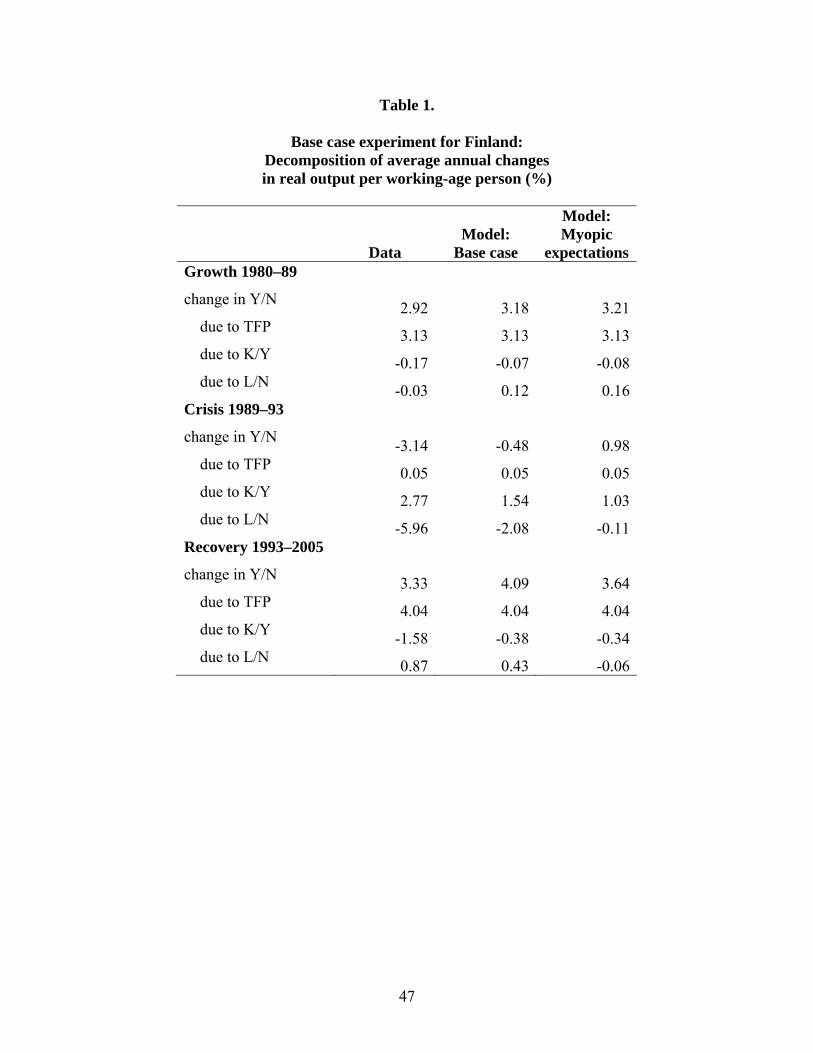
47

Table 1.

Base case experiment for Finland: Decomposition of average annual changes in real output per working-age person (%)

Data Model:

Base case

Model: Myopic

expectations Growth 1980–89

change in Y/N 2.92 3.18 3.21 due to TFP 3.13 3.13 3.13 due to K/Y -0.17 -0.07 -0.08 due to L/N -0.03 0.12 0.16 Crisis 1989–93 change in Y/N -3.14 -0.48 0.98 due to TFP 0.05 0.05 0.05 due to K/Y 2.77 1.54 1.03 due to L/N -5.96 -2.08 -0.11 Recovery 1993–2005 change in Y/N 3.33 4.09 3.64 due to TFP 4.04 4.04 4.04 due to K/Y -1.58 -0.38 -0.34 due to L/N 0.87 0.43 -0.06

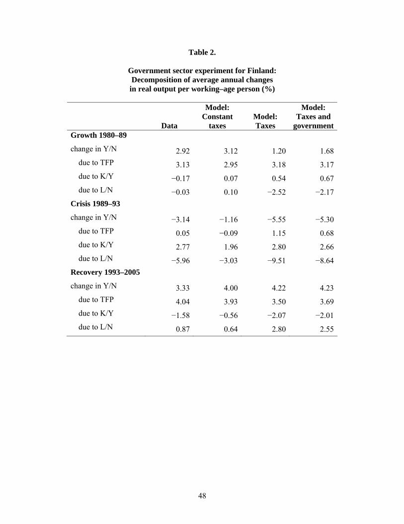
48

Table 2.

Government sector experiment for Finland: Decomposition of average annual changes in real output per working–age person (%)

Data

Model: Constant

taxes Model: Taxes

Model: Taxes and

governmentGrowth 1980–89

change in Y/N 2.92 3.12 1.20 1.68 due to TFP 3.13 2.95 3.18 3.17 due to K/Y −0.17 0.07 0.54 0.67 due to L/N −0.03 0.10 −2.52 −2.17Crisis 1989–93 change in Y/N −3.14 −1.16 −5.55 −5.30 due to TFP 0.05 −0.09 1.15 0.68 due to K/Y 2.77 1.96 2.80 2.66 due to L/N −5.96 −3.03 −9.51 −8.64Recovery 1993–2005 change in Y/N 3.33 4.00 4.22 4.23 due to TFP 4.04 3.93 3.50 3.69 due to K/Y −1.58 −0.56 −2.07 −2.01 due to L/N 0.87 0.64 2.80 2.55

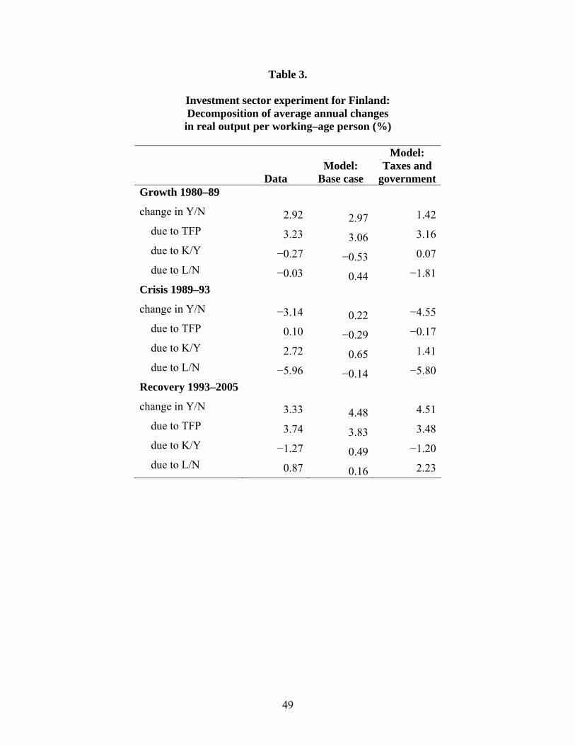
49

Table 3.

Investment sector experiment for Finland: Decomposition of average annual changes in real output per working–age person (%)

Data

Model: Base case

Model: Taxes and

government Growth 1980–89

change in Y/N 2.92 2.97 1.42 due to TFP 3.23 3.06 3.16 due to K/Y −0.27 −0.53 0.07 due to L/N −0.03 0.44 −1.81 Crisis 1989–93 change in Y/N −3.14 0.22 −4.55 due to TFP 0.10 −0.29 −0.17 due to K/Y 2.72 0.65 1.41 due to L/N −5.96 −0.14 −5.80 Recovery 1993–2005 change in Y/N 3.33 4.48 4.51 due to TFP 3.74 3.83 3.48 due to K/Y −1.27 0.49 −1.20 due to L/N 0.87 0.16 2.23

50

Table 4.

Foreign sector experiment for Finland: Decomposition of average annual changes in real output per working-age person (%)

Data

Model: Base case

Model: Exogenous

trade balance Growth 1980–89 change in Y/N 2.92 3.36 3.55 due to TFP 3.15 3.16 3.23 due to K/Y -0.19 -0.34 -0.19 due to L/N -0.03 0.54 0.51 Crisis 1989–93

change in Y/N -3.14 -1.60 -0.79 due to TFP 0.07 -0.47 -0.82 due to K/Y 2.75 2.00 2.38 due to L/N -5.96 -3.13 -2.35 Recovery 1993–2005

change in Y/N 3.33 3.97 3.81 due to TFP 4.06 4.31 4.47 due to K/Y -1.59 -0.62 -0.76 due to L/N 0.87 0.27 0.10

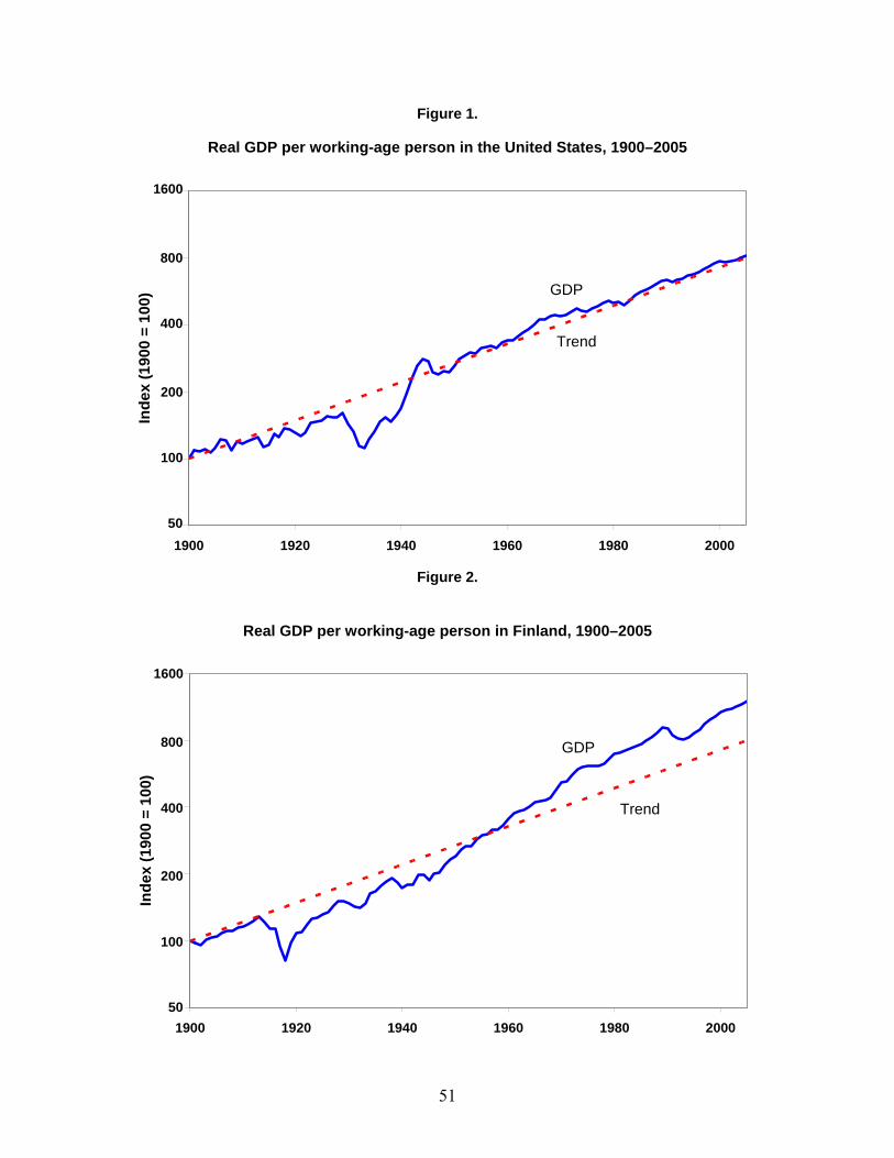
51

Figure 1.

Real GDP per working-age person in the United States, 1900–2005

-1

0

1

2

3

4

1900 1920 1940 1960 1980 2000

Inde

x (1

900

= 10

0)

50

100

200

400

800

1600

Trend

GDP

Figure 2.

Real GDP per working-age person in Finland, 1900–2005

-1

0

1

2

3

4

1900 1920 1940 1960 1980 2000

Inde

x (1

900

= 10

0)

50

100

200

400

800

1600

Trend

GDP

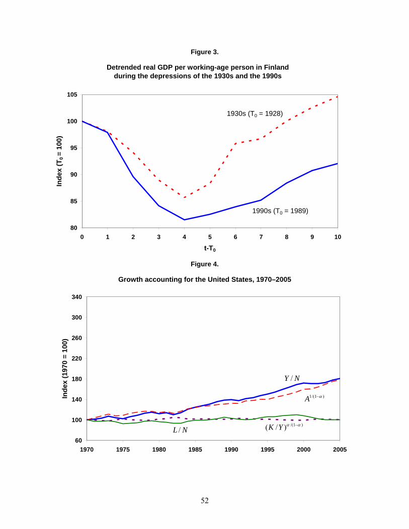
52

Figure 3.

Detrended real GDP per working-age person in Finland during the depressions of the 1930s and the 1990s

80

85

90

95

100

105

0 1 2 3 4 5 6 7 8 9 10

t-T0

Inde

x (T

0 =

100)

1930s (T0 = 1928)

1990s (T0 = 1989)

Figure 4.

Growth accounting for the United States, 1970–2005

60

100

140

180

220

260

300

340

1970 1975 1980 1985 1990 1995 2000 2005

Inde

x (1

970

= 10

0)

/L N/(1 )( / )K Y α α−

1/(1 )A α−

/Y N

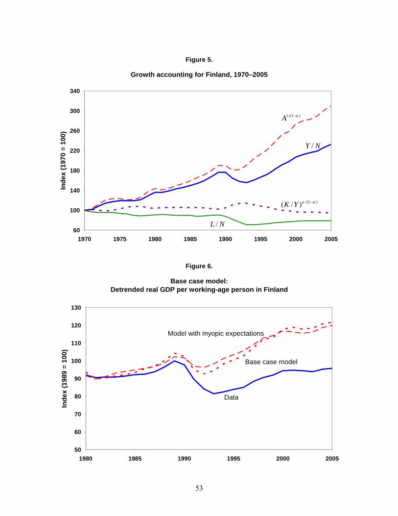
53

Figure 5.

Growth accounting for Finland, 1970–2005

60

100

140

180

220

260

300

340

1970 1975 1980 1985 1990 1995 2000 2005

Inde

x (1

970

= 10

0)

/L N

/(1 )( / )K Y α α−

1/(1 )A α−

/Y N

Figure 6.

Base case model: Detrended real GDP per working-age person in Finland

50

60

70

80

90

100

110

120

130

1980 1985 1990 1995 2000 2005

Inde

x (1

989

= 10

0)

Data

Base case model

Model with myopic expectations

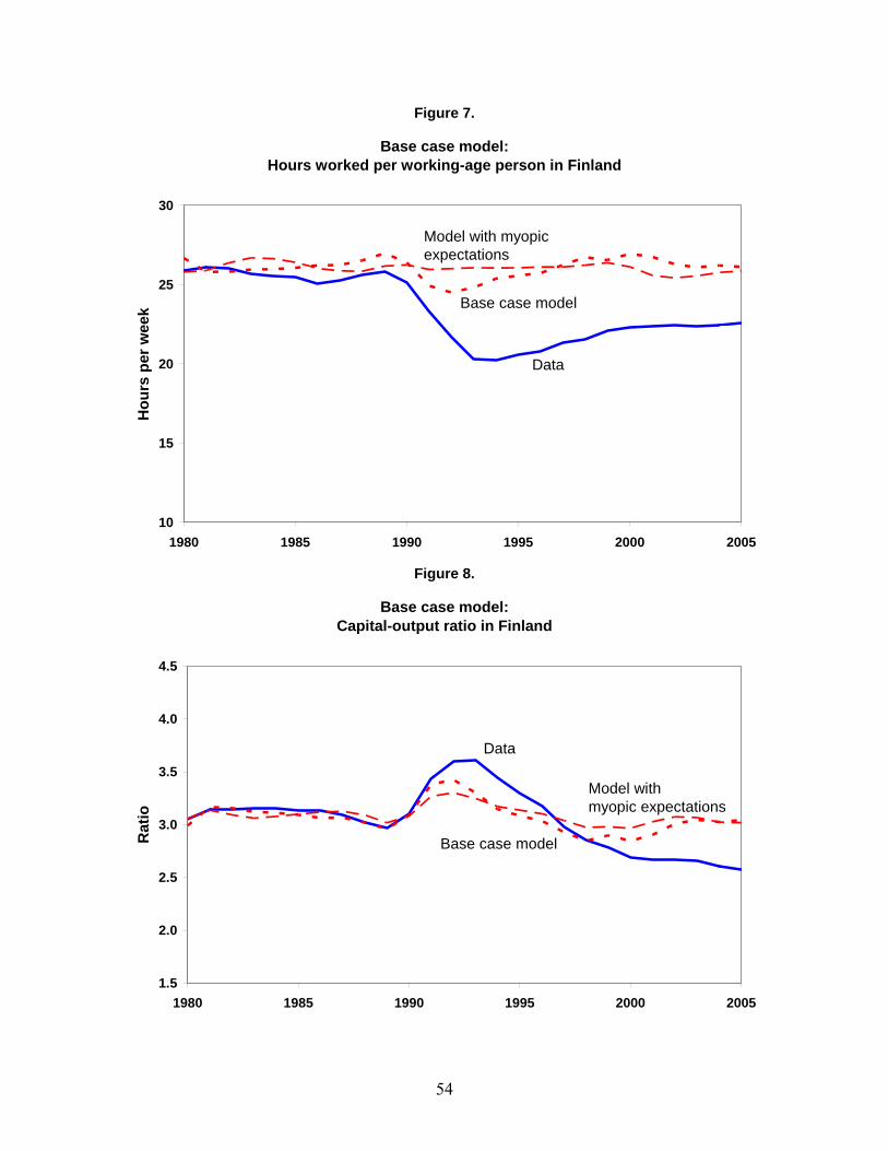
54

Figure 7.

Base case model: Hours worked per working-age person in Finland

10

15

20

25

30

1980 1985 1990 1995 2000 2005

Hou

rs p

er w

eek

Data

Model with myopic expectations

Base case model

Figure 8.

Base case model: Capital-output ratio in Finland

1.5

2.0

2.5

3.0

3.5

4.0

4.5

1980 1985 1990 1995 2000 2005

Rat

io

Data

Base case model

Model with myopic expectations

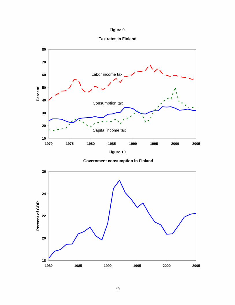
55

Figure 9.

Tax rates in Finland

10

20

30

40

50

60

70

80

1970 1975 1980 1985 1990 1995 2000 2005

Perc

ent

Labor income tax

Capital income tax

Consumption tax

Figure 10.

Government consumption in Finland

18

20

22

24

26

1980 1985 1990 1995 2000 2005

Perc

ent o

f GD

P

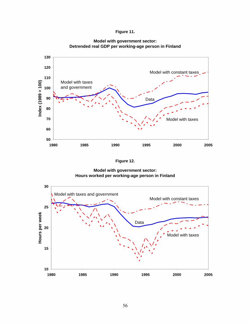
56

Figure 11.

Model with government sector: Detrended real GDP per working-age person in Finland

50

60

70

80

90

100

110

120

130

1980 1985 1990 1995 2000 2005

Inde

x (1

989

= 10

0)

Data

Model with taxes and government

Model with taxes

Model with constant taxes

Figure 12.

Model with government sector: Hours worked per working-age person in Finland

10

15

20

25

30

1980 1985 1990 1995 2000 2005

Hou

rs p

er w

eek

Data

Model with taxes and government

Model with taxes

Model with constant taxes

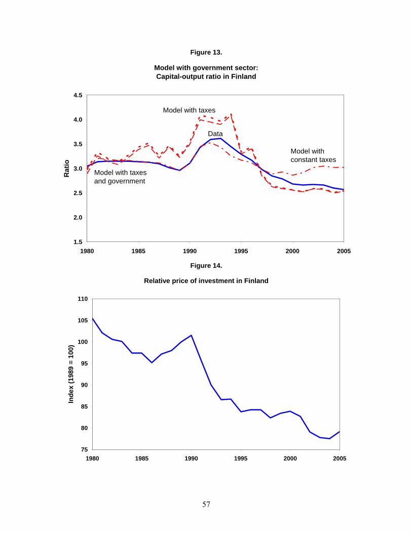
57

Figure 13.

Model with government sector: Capital-output ratio in Finland

1.5

2.0

2.5

3.0

3.5

4.0

4.5

1980 1985 1990 1995 2000 2005

Rat

io

Data

Model with taxes and government

Model with taxes

Model with constant taxes

Figure 14.

Relative price of investment in Finland

75

80

85

90

95

100

105

110

1980 1985 1990 1995 2000 2005

Inde

x (1

989

= 10

0)

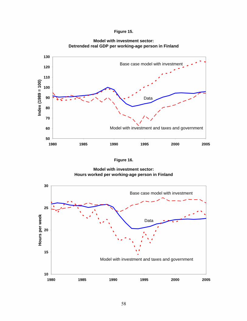
58

Figure 15.

Model with investment sector: Detrended real GDP per working-age person in Finland

50

60

70

80

90

100

110

120

130

1980 1985 1990 1995 2000 2005

Inde

x (1

989

= 10

0)

Data

Model with investment and taxes and government

Base case model with investment

Figure 16.

Model with investment sector: Hours worked per working-age person in Finland

10

15

20

25

30

1980 1985 1990 1995 2000 2005

Hou

rs p

er w

eek

Data

Base case model with investment

Model with investment and taxes and government

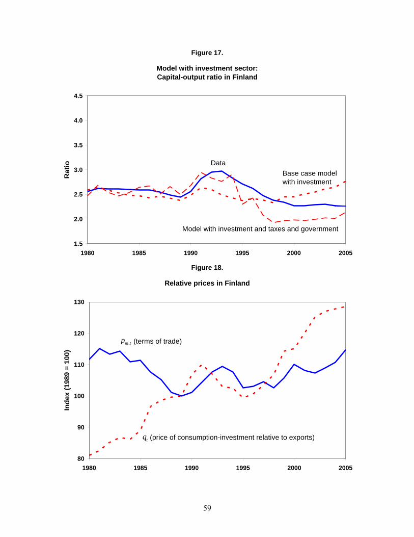
59

Figure 17.

Model with investment sector: Capital-output ratio in Finland

1.5

2.0

2.5

3.0

3.5

4.0

4.5

1980 1985 1990 1995 2000 2005

Rat

io Data

Model with investment and taxes and government

Base case modelwith investment

Figure 18.

Relative prices in Finland

80

90

100

110

120

130

1980 1985 1990 1995 2000 2005

Inde

x (1

989

= 10

0)

(terms of trade),m tp

(price of consumption-investment relative to exports)tq

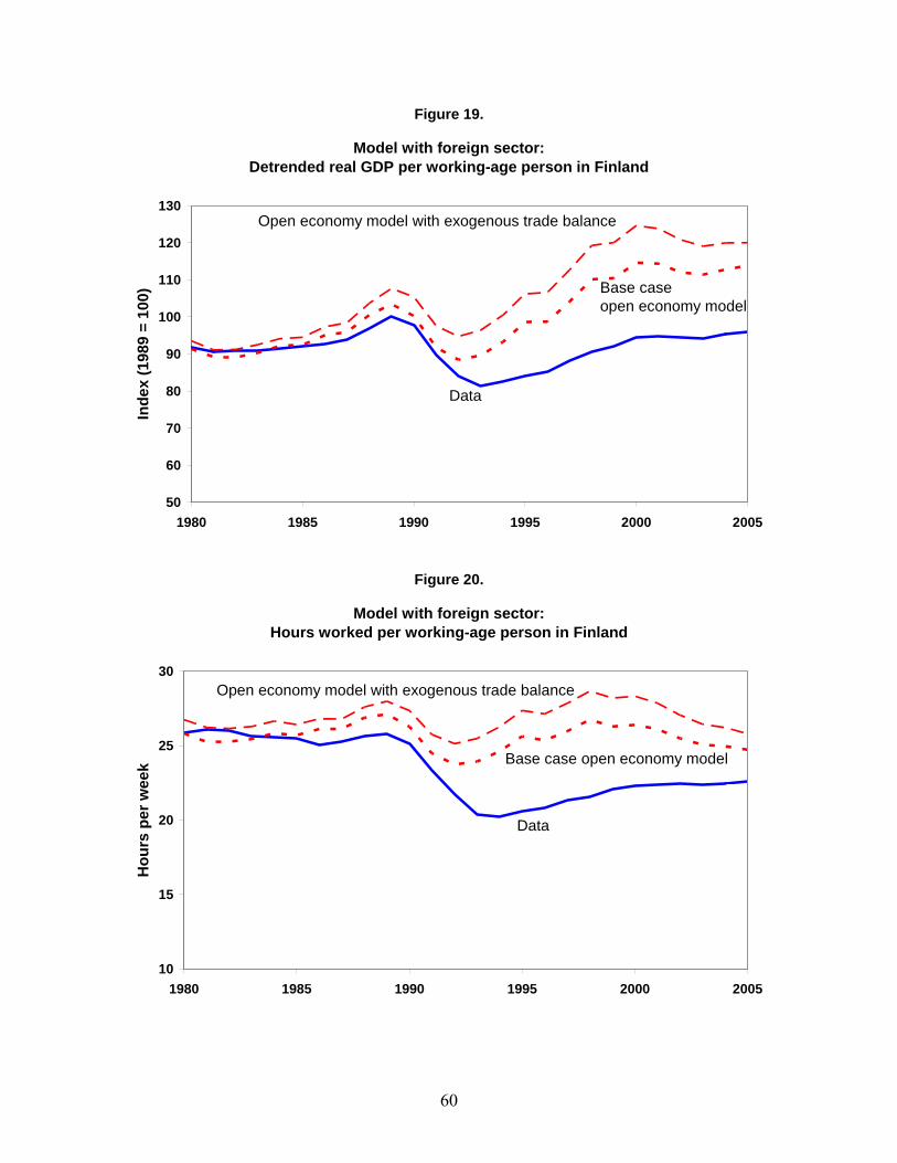
60

Figure 19.

Model with foreign sector: Detrended real GDP per working-age person in Finland

50

60

70

80

90

100

110

120

130

1980 1985 1990 1995 2000 2005

Inde

x (1

989

= 10

0)

Data

Open economy model with exogenous trade balance

Base case open economy model

Figure 20.

Model with foreign sector: Hours worked per working-age person in Finland

10

15

20

25

30

1980 1985 1990 1995 2000 2005

Hou

rs p

er w

eek

Data

Open economy model with exogenous trade balance

Base case open economy model

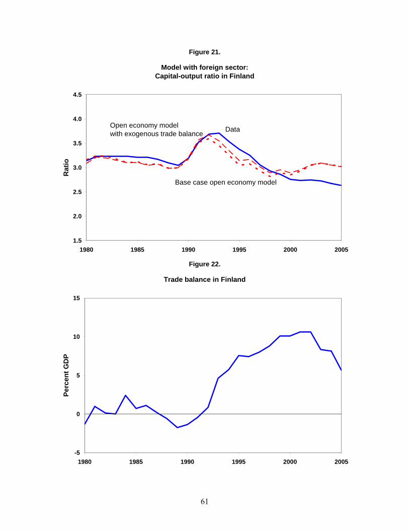
61

Figure 21.

Model with foreign sector: Capital-output ratio in Finland

1.5

2.0

2.5

3.0

3.5

4.0

4.5

1980 1985 1990 1995 2000 2005

Rat

io

Data

Base case open economy model

Open economy model with exogenous trade balance

Figure 22.

Trade balance in Finland

-5

0

5

10

15

1980 1985 1990 1995 2000 2005

Perc

ent G

DP

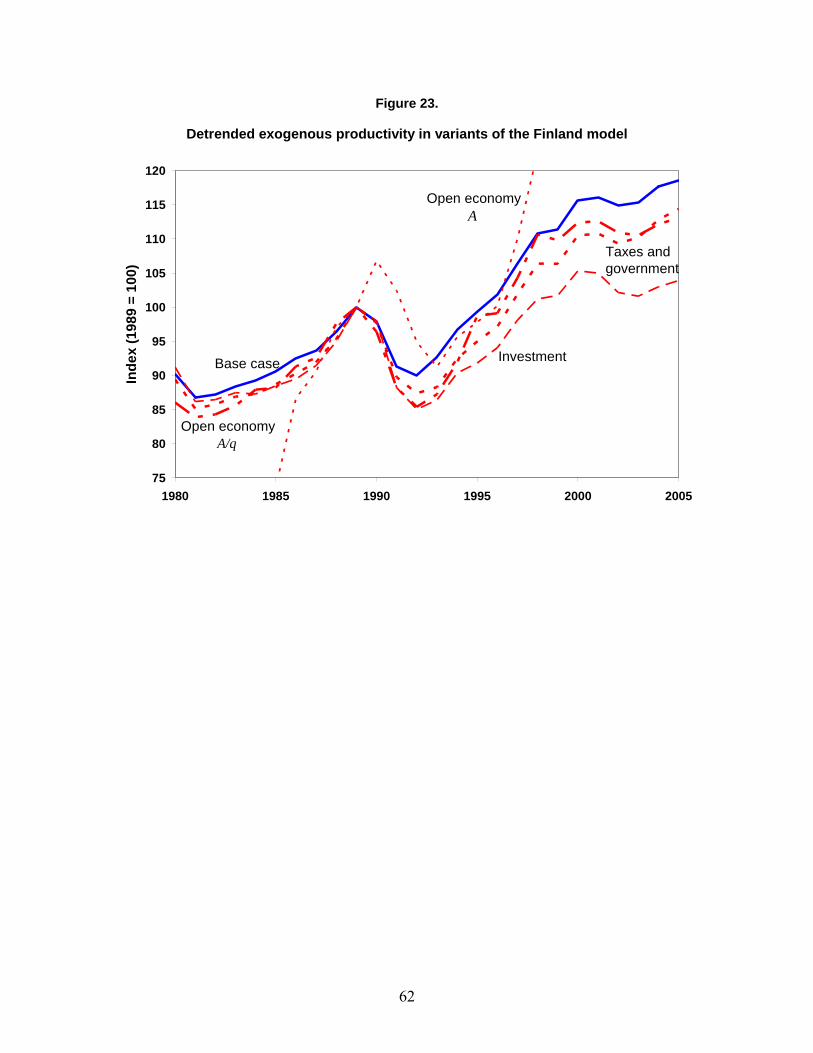
62

Figure 23.

Detrended exogenous productivity in variants of the Finland model

75

80

85

90

95

100

105

110

115

120

1980 1985 1990 1995 2000 2005

Inde

x (1

989

= 10

0)

InvestmentBase case

Taxes and government

Open economy A/q

Open economy A