Getting started-with-lotus-vehicle-simulation

GETTING STARTED USING LOTUS VEHICLE SIMULATION

V E R S I O N 3 .11

The information in this document is furnished for informational use only, may be revised from time to time, and should not be construed as a commitment by Lotus Cars Ltd or any associated or subsidiary company. Lotus Cars Ltd assumes no responsibility or liability for any errors or inaccuracies that may appear in this document. This document contains proprietary and copyrighted information. Lotus Cars Ltd permits licensees of Lotus Cars Ltd software products to print out or copy this document or portions thereof solely for internal use in connection with the licensed software. No part of this document may be copied for any other purpose or distributed or translated into any other language without the prior written permission of Lotus Cars Ltd. ©2001 by Lotus Cars Ltd. All rights reserved.

Getting Started Using Lotus Vehicle Simulation Contents

i

Contents About This Guide iii Welcome to Lotus Vehicle Simulation iii What you Need to Know iii Chapter 1. Introducing Lotus Vehicle Simulation 1 Overview 1 What is Lotus Vehicle Simulation? 2 Lotus Vehicle Simulation Structure 3 Getting Help Using Lotus Vehicle Simulation 5 Chapter 2. Tutorial 1, ‘Building a Lotus Vehicle Simulation Model’ 7 Overview 7 Starting Lotus Vehicle Simulation 8 Familiarising yourself with Lotus Vehicle simulation 9 Inputting Values into the Data Modules 10 Data Checking 22 Running an Acceleration Simulation 24 Displaying the Simulation Results 27 Chapter 3. Tutorial 2, ‘Steady Speed Solver Application’ 31 Overview 31 Opening an example *.car file 32 View Selected Data Modules 33 Running the Steady Speed Solve 38 Displaying the Simulation Results 39 Analysing the Simulation Results 40 An Alternative analysis Method – Batch Analysis 41 Chapter 4. Tutorial 3, ‘Acceleration Solver Application’ 43 Overview 43 Opening an example *.car file 44 Running the Acceleration Solver 45 Calculation Set-Up 45 Displaying the Simulation Results 46 An Extension to the Batch Analysis Approach 48 Chapter 5. Tutorial 4, ‘Emissions Cycle Solver Application’ 51 Overview 51 Opening an example *.car file 52 Running the Emissions Cycle Solver 54 Calculation Set-Up 54 Displaying the Simulation Results 55 X-Y Results Plotting 56 Use of the Parametric Analysis Tool 58

Getting Started Using Lotus Vehicle Simulation Contents

ii

Chapter 6. Tutorial 5, ‘Track Solver Application’ 61 Overview 61 Opening an example *.car file 62 Running the Track Solver 63 Calculation Set-Up 64 Displaying the Simulation Results 64 3D Viewing of the Results 65 Use of the DataBase Tool 66 Use of the Parametric Analysis Tool for Multi-Variant analysis 68

Getting Started Using Lotus Vehicle Simulation About This Guide

iii

About This Guide Welcome to Lotus Vehicle Simulation Welcome to Lotus Vehicle Simulation. Using Lotus Vehicle Simulation, you can build virtual vehicle models and analyses their performance over a range of different simulation cycle types, from simple fixed speed runs to accelerations and emissions cycles.

What You Need to Know This guide assumes the following: n Lotus Vehicle Simulation is installed on your computer or network and

you have permission to execute Lotus Vehicle Simulation module.

n The necessary password files are installed to allow you to run the necessary modules.

n You have a basic understanding of vehicle motion, and the relevance and limitations of the required component data variables.

Getting Started Using Lotus Vehicle Simulation About this Guide

iv

Introducing Lotus Vehicle Simulation

1

Overview This chapter introduces you to Lotus Vehicle Simulation and explains the benefits of the code. It also explains how you can learn more about Lotus Vehicle Simulation and introduces tutorials that will help you to get started. This chapter contains the following sections:

n What is Lotus Vehicle Simulation?, 2

n Lotus Vehicle Simulation Structure, 3

n Getting Help Using Lotus Vehicle Simulation, 5

Getting Started Using Lotus Vehicle Simulation Introducing Lotus Vehicle Simulation

2

What is LOTUS VEHICLE SIMULATION? LOTUS VEHICLE SIMULATION is a simulation program capable of predicting the complete performance of a vehicle system. The program can be used to calculate,

• Straight line acceleration and top speed • Fuel economy and emissions (both in steady state or across any drive-cycle) • Track or course performance

Lotus Vehicle Simulation is designed to run on a desktop PC with Windows NT/98 but offers the speed of a UNIX based simulation. The user interface is based on the standard Lotus software ‘look-and-feel’ and offers the same intuitive approach as other popular Windows applications, assisting learning and speed of use. Using the simulation program typically follows the procedure below,

• The user constructs a simulation model by entering the vehicle specification. This includes data for :

Ø Vehicle mass and centre of gravity Ø Vehicle dimensions, and aerodynamics Ø Tyre performance Ø Final drive system Ø Gearbox or transmission system and shifting strategies Ø Prime mover details eg. I.C. engine or hybrid powertrain Ø Performance (torque/power capabilities) Ø Fuel economy Ø System-out Emissions Ø Emissions after-treatment systems Ø Driver performance

• The user selects the appropriate test for analysis. For instance, this often involves

predicting the performance of the vehicle in terms of emissions and fuel economy over a government legislated drive-cycle.

• The calculation cycle is carried out. The user can display the key information on the

vehicle and powertrain operating condition during the cycle using the calculation screen.

• Calculation results are available to the user both in the form of a report quality

summary sheet and through a quick-to-use graph plotting system. Lotus Vehicle Simulation has been applied extensively by world-wide clients and validated thoroughly at Lotus over a wide range of vehicle types and conditions. The program is capable of simulating all existing and projected vehicle systems and is continually updated by Lotus in co-operation with it’s partners.


3

Lotus Vehicle Simulation structure Lotus Vehicle Simulation is split into three sub-sections:

• Data module - data-entry and model generation • Solve module - solution of desired analysis • Results module - analysis of calculated results

The three sections are only notionally split and all three modules run together as a single application.

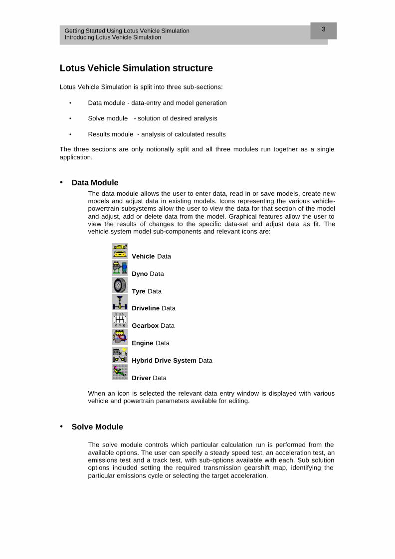
• Data Module The data module allows the user to enter data, read in or save models, create new models and adjust data in existing models. Icons representing the various vehicle-powertrain subsystems allow the user to view the data for that section of the model and adjust, add or delete data from the model. Graphical features allow the user to view the results of changes to the specific data-set and adjust data as fit. The vehicle system model sub-components and relevant icons are:

Vehicle Data

Dyno Data

Tyre Data

Driveline Data

Gearbox Data

Engine Data

Hybrid Drive System Data

Driver Data

When an icon is selected the relevant data entry window is displayed with various vehicle and powertrain parameters available for editing.

• Solve Module

The solve module controls which particular calculation run is performed from the available options. The user can specify a steady speed test, an acceleration test, an emissions test and a track test, with sub-options available with each. Sub solution options included setting the required transmission gearshift map, identifying the particular emissions cycle or selecting the target acceleration.


4

• Results Module

The results module is used to perform all post-processing of calculated data. It provides the following features:

• Plotting of data sets - Up to five runs simultaneously • Plotting of multiple data-channels e.g. Vehicle fuel consumption and

forward speed vs. time - up to 4 sets • Cross plotting of data sets and channels on a single multi-axis graph • Zoom and pick functions

The Windows environment also allows frame grabbing of graphs as bitmaps for pasting into other Windows applications.


5

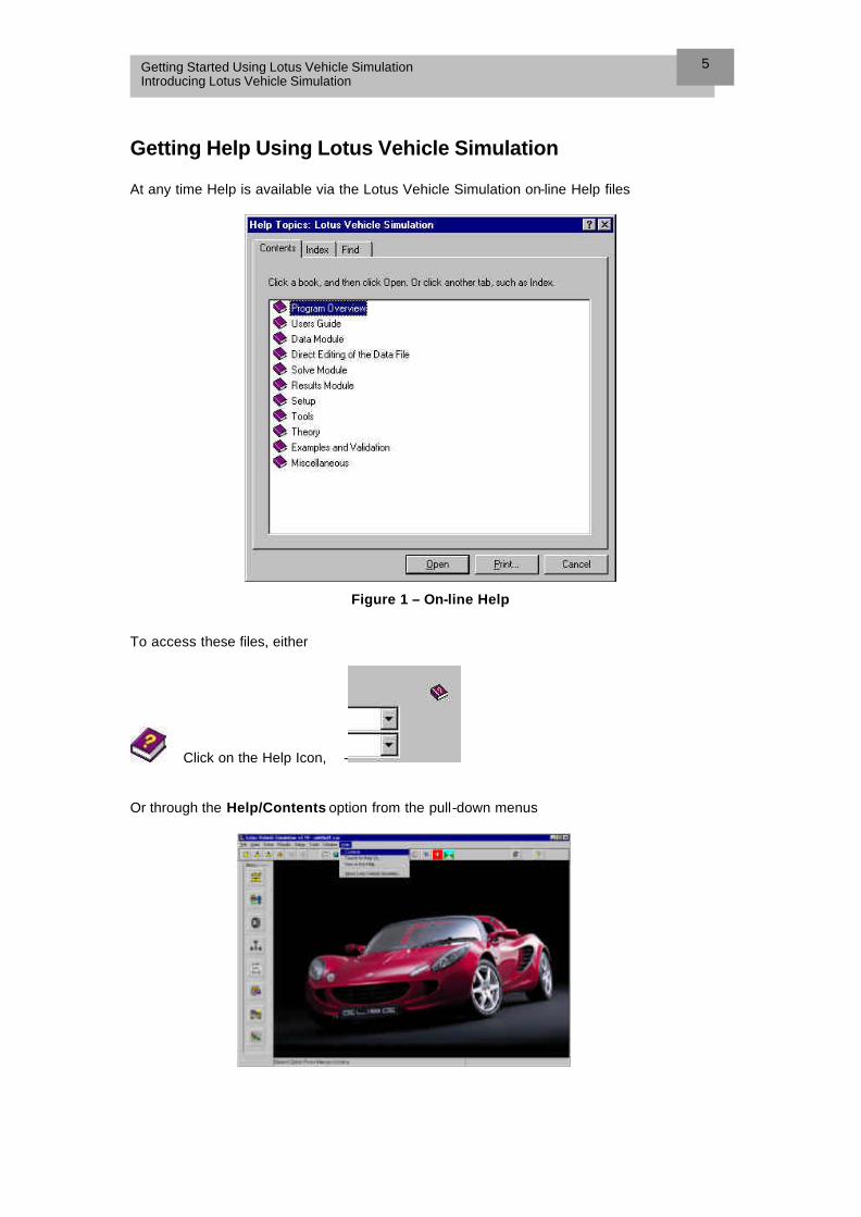
Getting Help Using Lotus Vehicle Simulation At any time Help is available via the Lotus Vehicle Simulation on-line Help files

Figure 1 – On-line Help

To access these files, either

Click on the Help Icon, - Or through the Help/Contents option from the pull-down menus


6

Tutorial 1 - Building a Lotus Vehicle Simulation Model 2

Overview The following chapter provides a new user with all the information required to open, build and simulate a new Lotus Vehicle Simulation model. This chapter includes the following sections: n Starting Lotus Vehicle Simulation, 8

n Familiarising yourself with Lotus Vehicle Simulation, 9

n Inputting Values into the Data Modules, 10

n Data Checking, 22

n Running an Acceleration Simulation, 24

n Displaying the simulation results via:, 27

- Results Text File Viewer

This Tutorial takes approximately 1½ hour to complete

Getting Started Using Lotus Vehicle Simulation Tutorial 1 – Building a Lotus Vehicle Simulation model

8

Starting LOTUS VEHICLE SIMULATION To start LOTUS VEHICLE SIMULATION in the windows environment

• From the Desktop Icon

During the program install, a LOTUS VEHICLE SIMULATION icon will be added to the Windows desktop Double click on the LOTUS VEHICLE SIMULATION icon to display the Startup Wizard dialog box as shown below

• From the Start Menu

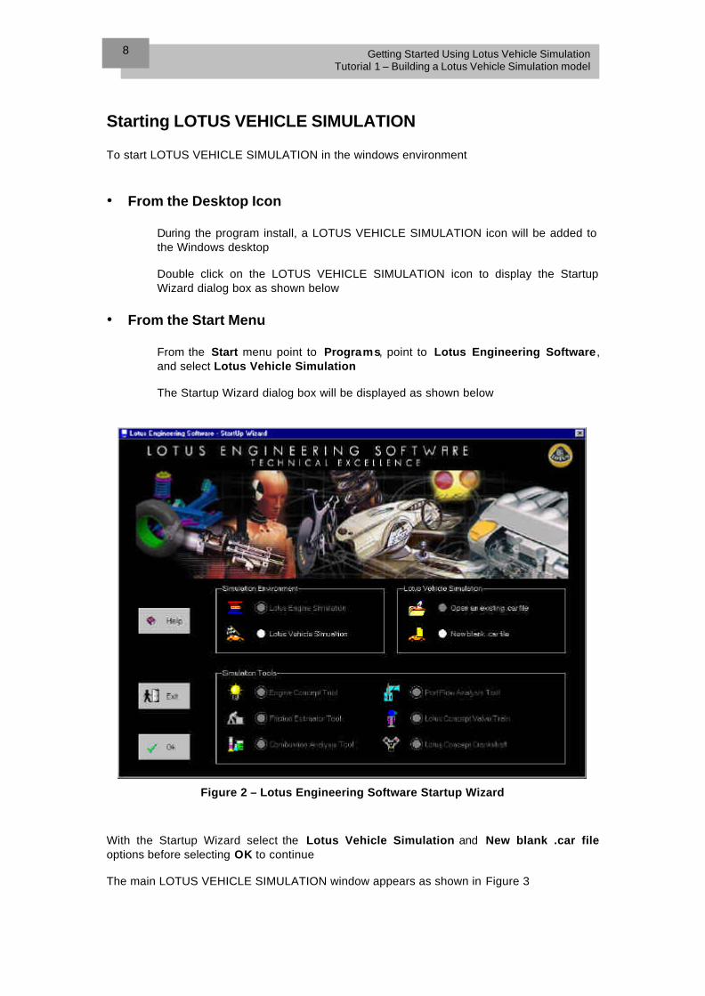
From the Start menu point to Programs, point to Lotus Engineering Software , and select Lotus Vehicle Simulation The Startup Wizard dialog box will be displayed as shown below

Figure 2 – Lotus Engineering Software Startup Wizard

With the Startup Wizard select the Lotus Vehicle Simulation and New blank .car file options before selecting OK to continue The main LOTUS VEHICLE SIMULATION window appears as shown in Figure 3


9

Familiarising yourself with LOTUS VEHICLE SIMULATION Before continuing any further, take some time to familiarise yourself with the LOTUS VEHICLE SIMULATION main window

Figure 3 – Lotus Engineering Software Main Window

In particular note the following

♦ The data module icons on the left hand side of the main window. These icons representing the various vehicle-powertrain subsystems, which allow the user to view the data for that section of the model and adjust, add or delete data from the model.

♦

The file management icons on the top left of the toolbar. These icons are used to generate new model file and open and save existing files

♦

The solve module icons in the middle of the toolbar. These icons allow the user to select which particular calculation run is performed from the available options

♦

The results module icons on the top right of the toolbar. These icons allow the user to select the type of simulation results viewer


10

Inputting Values into the Data Modules This section will describe the step by step process of entering data into a new LOTUS VEHICLE SIMULATION model. With all the data modules described below the following options are available to assist the user.

Where relevant a graphical representation of the data can be displayed by clicking on the graphics icon in the top right of the data window

On-line help can be displayed by clicking on the help icon in the top right of the data window

We will now input some example vehicle data into the individual data modules

1 Vehicle Data

Select the Vehicle data input window. This window is accessed using the Vehicle icon on the tool bar or through the Data/Vehicle option from the pull-down menus or press F1.

The vehicle data windows will appear as shown below

Figure 4 – Vehicle Data Window

Populate the vehicle data window by inputting the following examples into the appropriate text boxes. All the input variables may not be required for a basic simulation, where this is the case a * symbol is used in the example data table and the text box can be left blank (see the LOTUS VEHICLE SIMULATION User’s manual for more information)

i


11

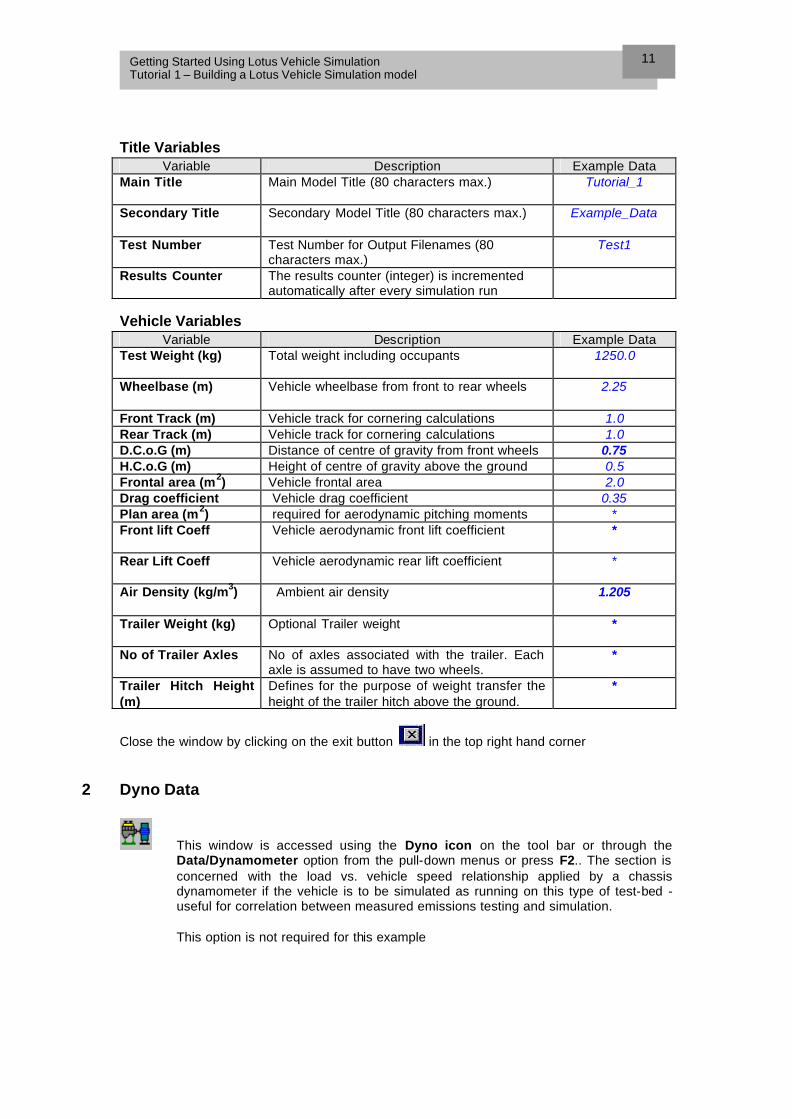
Title Variables

Variable Description Example Data Main Title

Main Model Title (80 characters max.) Tutorial_1

Secondary Title

Secondary Model Title (80 characters max.) Example_Data

Test Number Test Number for Output Filenames (80 characters max.)

Test1

Results Counter The results counter (integer) is incremented automatically after every simulation run

Vehicle Variables

Variable Description Example Data Test Weight (kg)

Total weight including occupants 1250.0

Wheelbase (m)

Vehicle wheelbase from front to rear wheels 2.25

Front Track (m) Vehicle track for cornering calculations 1.0 Rear Track (m) Vehicle track for cornering calculations 1.0 D.C.o.G (m) Distance of centre of gravity from front wheels 0.75 H.C.o.G (m) Height of centre of gravity above the ground 0.5 Frontal area (m2) Vehicle frontal area 2.0 Drag coefficient Vehicle drag coefficient 0.35 Plan area (m2) required for aerodynamic pitching moments * Front lift Coeff

Vehicle aerodynamic front lift coefficient *

Rear Lift Coeff

Vehicle aerodynamic rear lift coefficient *

Air Density (kg/m3)

Ambient air density 1.205

Trailer Weight (kg)

Optional Trailer weight *

No of Trailer Axles No of axles associated with the trailer. Each axle is assumed to have two wheels.

*

Trailer Hitch Height (m)

Defines for the purpose of weight transfer the height of the trailer hitch above the ground.

*

Close the window by clicking on the exit button in the top right hand corner

2 Dyno Data

This window is accessed using the Dyno icon on the tool bar or through the Data/Dynamometer option from the pull-down menus or press F2.. The section is concerned with the load vs. vehicle speed relationship applied by a chassis dynamometer if the vehicle is to be simulated as running on this type of test-bed - useful for correlation between measured emissions testing and simulation.

This option is not required for this example


12

Save the model for the first time.

To save the select model use File/Save As from the menu-bar or the file save as icon from the main window tool-bar. This will automatically bring up the browser and prompt the user to enter a new filename

Figure 5 – Save As Window

Save the model as tutorial1.car

3 Tyre Data

Select the Tyre data input window. This window is accessed using the Tyre icon on the tool bar or through the Data/Tyre option from the pull-down menus or press F3.. The tyre window is concerned with the load vs. vehicle speed relationship for tyre rolling resistance and the definition of tyre rolling radius and efficiency.

The tyre data windows will appear as shown below

Figure 6 – Vehicle Data Window

i


13

The tyre model is a pre-requisite of the simulation and hence cannot be switched off. To select default Lotus values for the tyre rolling resistance curve coefficients select from the tyre data menubar the CopyData / Set Rolling Resistance to Default Values.

Figure 7 – Vehicle Data Window – Set Rolling Resistance to Default Values

The tyre data can be defined for both front, rear and trailer tyres separately or as a common tyre. Select the common tyre option from the drop down list box

Figure 8 – Vehicle Data Window – Selecting Common Tyre Option

Populate the tyre data window by inputting the following example data into the appropriate text boxes. Tyre Variables

Variable Description Example Data Rolling Radius (m)

The tyre rolling radius Note: using the tyre unloaded radius is an approximation

0.284

Drive Efficiency (0-1)

Tyre transmission efficiency - typically ~ 0.95 0.95

Coeff of Slip (u)

Coefficient of friction between the tyre and the road. Typically in the range 0.8 - 1.15.

1.0



14

Save the model.

To save a model, select the file save iconfrom the main window tool-bar or the menu-bar option File/Save. If no change has been made to the model, this automatically brings up the browser to add a new file-name. Otherwise the file is overwritten.

4 Driveline Data

Select the Driveline data input window. This window is accessed using the Driveline icon on the tool bar or through the Data/Driveline option from the pull-down menus or press F4. This action will call into view the driveline sub-menu which provides access to the various driveline data-windows as listed below:

Torque Converter/Clutch - Options for torque converters and clutches Torque Converter Lock-up - Definition of torque converter lock-up characteristics Torque Converter Idle - Definition of torque converter idle strategy Final Drive - Specification of final drive system, system inertia’s, transmission efficiencies and drive ratio.

4.1

Select TC/Clutch from the Driveline sub-menu, this will display the Drivetrain couple window shown in Figure 9 The example model we are building is fitted with a clutch, so select the clutch model from the ‘Options’ drop down list box.

Figure 9 – Drivetrain Couple Window – Clutch or Torque Converter Option

i


15

Populate the clutch data window by inputting the following example data into the appropriate text boxes. Clutch Variables

Variable Description Example Data Declutch Speed’ (km/h

Speed below which the clutch is decoupled from the engine

5.0


4.2 The Torque Converter Lock-up and Torque Converter Idle options from the Driveline sub-menu are not required as we have chosen a clutch model

4.3

Selected Final Drive from the Driveline sub-menu, this will display the final drive data window shown below in Figure 10

The example model we are building is a rear wheel drive vehicle so select the Rear -WD option from the ‘Drive Type’ drop down list box.

Figure 10 – Drivetrain Couple Window – Final Drive Data

Populate the final drive data window by inputting the following example data into the appropriate text boxes. Final Drive Variables

Variable Description Example Data Front Wheel Inertia (kg.m2)

The combined inertia of the wheel, tyre and rotating brakes etc. These are for a single wheel. Two wheels are assumed to be fitted.

0.6

Rear Wheel Inertia The combined inertia of the wheel, tyre and 0.6


16

(kg.m2)

rotating brakes etc. These are for a single wheel. Two wheels are assumed to be fitted.

Drive Shaft Inertia (kg.m2)

The rotary inertia of the axle/drive shaft. This is the total inertia if two drive shafts are fitted

0.01

Prop Shaft Inertia (kg.m2) :

Total rotary inertia of the prop shaft. If not fitted, set to zero.

0.05

Final Drive Ratio

Final Drive Gear Ratio 3.55

Final Drive Efficiency (0-1)

Maximum efficiency of the final drive used by transmission efficiency calculations

0.95

Final Drive Efficiency Mode

The user may choose between two different efficiency models : 1. Efficiency fixed to maximum 2. Efficiency modelled as a function of speed

and load

Fixed

Close the window and the Driveline sub-menu by clicking on the exit button in the top right hand corner

Save the model.

5 Gearbox Data

Select the Gearbox menu. To enter or review data for the gearbox, select the Gearbox Icon from the icon panel. Alternatively, select Data / Gearbox from the main window menu bar or press F5.

This brings up the gearbox menu from which the user can select from the following sub-window options:

Specification: where gearbox transmission type and ratios are entered Gear Losses: to enter detailed information on the system efficiency Shift Strategy: to enter information on the system operating strategy Cascade: to display a graphical representation of the drive force vs. Vehicle speed and road load Gradability: A calculation tool to assess the vehicle’s capabilities on inclines. Max. Speed: A similar tool to assess the Vehicle system’s maximum Speed

5.1

i


17

Select Specification from the Gearbox sub-menu, this will display the gearbox specification window shown below. This window allows the user to review the gearbox ratios, efficiencies and inertia’s

Figure 11 – Gearbox Specification Window

Populate the final drive data window by inputting the following example data into the appropriate text boxes. Final Drive Variables

Variable Description Example Data Number of Ratios

This specifies the number of ratios in the transmission. To initially set the number change the number from zero to the required number of ratios. This activates the spreadsheet and allows entry of data for each ratio.

5

Maximum Gearbox Input Torque (Nm)

This sets the maximum gearbox input torque. This is used by the gearbox efficiency calculations. If 0.0 is used, the calculation uses engine maximum torque

0.0

Maximum Gearbox Input Speed (rpm)

This sets the gearbox maximum input speed. This is used by the gearbox efficiency calculations. If 0.0 is used, the calculation uses engine maximum speed.

0.0

Gearbox Efficiency Model

The user may choose between two different efficiency models : 1. Efficiency fixed to maximum (entered

value) 2. Efficiency modelled as a function of speed

and load using Lotus developed models.

Fixed

System Data Spreadsheets The spreadsheet on the right hand side of the gear specification window is used to enter data for the characteristics of each gear ratio. The number of ratios in the model is set using the gearbox ‘number of ratios’ data box.


18

• Using Spreadsheets To manipulate data in a spreadsheet, for instance in the gear specification window, first ensure that a spreadsheet is available. If not, then go to the number of ratios text box and enter the required gear ratios To copy a section of data, drag the pointer across the section and with the area highlighted, press the right button. This calls a pointer pop-down menu to access the copy option. Then moving to the desired cell, select it and repeat the menu selection procedure choosing paste.

Figure 12 – Gearbox Specification Window

Populate the spreadsheet with the following example data, as shown in Figure 13 below: The three variables for each gear are as follows: Ratio: Specifies the ratio of input to output speed for each ratio. Efficiency: Specifies the efficiency of each ratio as a fraction of 1.0. Inertia: Specifies the rotational inertia of each ratio (kg.m2) Overall Ratio: This is the automatically calculated product of gear and final drive ratios

Figure 13 – Gearbox Specification Example Data When you have finished entering this data close the gearbox specification window by clicking

on the exit button in the top right hand corner

5.2

The Gear Losses, Shift Strategy, Cascade, Gradability and Max.Speed options from the Gearbox sub-menu are not required for this model application. For more information on these options consult the Data Modules section of the LOTUS VEHICLE SIMULATION User’s Manual

i


19

Close the Gearbox sub-menu by clicking on the exit button in the top right hand corner

Save the model.

6 Engine Data

Select the Engine data -menu. To enter or review data for the engine, select the Engine Icon from the icon panel. Alternatively, select Data / Engine from the main window menu bar or press F6.

The engine data section forms the primary data screens for data entry to define the central powertrain unit. The following sub-window options are available

Engine : Data for the I.C. Engine specification, inertia and full-load performance. Engine Scaling : Advanced tool to adjust engine specification via scaling functions. Engine Maps : Data window for full and part load fuel economy, emissions and engine operating condition. Optimum: Tool to calculate optimum load-speed profile to minimise any selected map parameter - can then be used to drive shift strategy. Catalyst: Data window for catalyst light-off characteristics and emissions after-treatment efficiency. Warm-up: Data window for engine-out emissions and fuel economy during warm-up phase and engine acceleration. Auxiliaries: Data window for specification and load characteristics of powertrain mounted auxiliary devices. Grid Analysis: Data window for creation of a zone system for cumulative analysis of vehicle system operation across powertrain load-speed range. Primary Drive : Data window for specification of engine primary drive, inertia and efficiency. Units: Window for selection of preferred displayed units

6.1

Select Engine from the Engine sub-menu, this will display the engine data window, as shown in Figure 14, which is used to review or adjust engine data

i


20

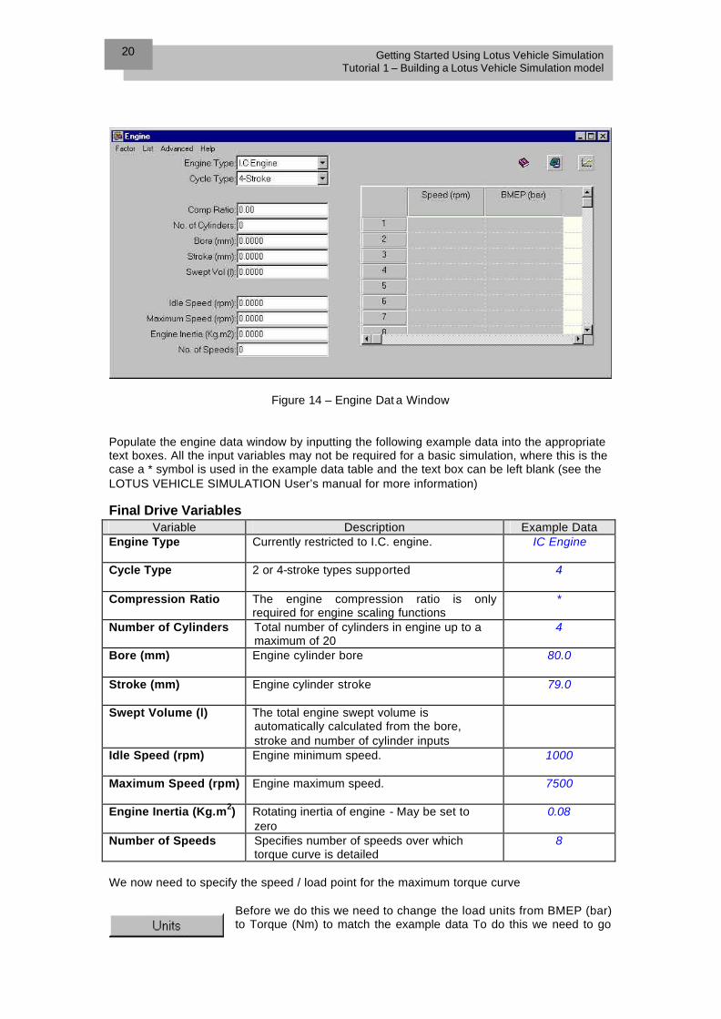
Figure 14 – Engine Dat a Window

Populate the engine data window by inputting the following example data into the appropriate text boxes. All the input variables may not be required for a basic simulation, where this is the case a * symbol is used in the example data table and the text box can be left blank (see the LOTUS VEHICLE SIMULATION User’s manual for more information) Final Drive Variables

Variable Description Example Data Engine Type

Currently restricted to I.C. engine. IC Engine

Cycle Type

2 or 4-stroke types supported 4

Compression Ratio The engine compression ratio is only required for engine scaling functions

*

Number of Cylinders

Total number of cylinders in engine up to a maximum of 20

4

Bore (mm)

Engine cylinder bore 80.0

Stroke (mm)

Engine cylinder stroke 79.0

Swept Volume (l) The total engine swept volume is automatically calculated from the bore, stroke and number of cylinder inputs

Idle Speed (rpm) Engine minimum speed.

1000

Maximum Speed (rpm) Engine maximum speed.

7500

Engine Inertia (Kg.m2) Rotating inertia of engine - May be set to zero

0.08

Number of Speeds Specifies number of speeds over which torque curve is detailed

8

We now need to specify the speed / load point for the maximum torque curve

Before we do this we need to change the load units from BMEP (bar) to Torque (Nm) to match the example data To do this we need to go


21

back to the engine menu and select the Units option, This will display the Units windows shown below:

Figure 15 – Units Window

Select the TORQUE (NM) option from the Load Units drop down menu. This will change the units in the input spreadsheet on the engine data window (Figure 14). Close the Units window

by clicking on the exit button in the top right hand corner Return to the engine data window, notice that the load units have now changed We can now populate the engine data spreadsheet with the following example data, as shown in Figure 16 below. The three variables for each gear are as follows: Speed (rpm): Specifies the engine rotational speed Torque (Nm): Specifies the maximum torque a the specified engine speed

Figure 16 – Engine Maximum Torque Curve Example Data

• Displaying the torque curve graphically The torque curve can be displayed graphically using the graph icon at the top right of the window. Try the zoom, autoscaling, data pick and printing features accessed from the pull-down menu at the top left of the graphic window.

i


22

Close the Engine Window by clicking on the exit button in the top right hand corner

6.2 The remaining options from the engine menu are not required for this model application. For more information on these options consult the Data Modules section of the LOTUS VEHICLE SIMULATION User’s Manual

Close the Engine-menu by clicking on the exit button in the top right hand corner

You have now complete inputting information for the example model.

7/8 Hybrid Drive System Data and Driver Data

The remaining data modules Hybrid Drive System Data and Driver Data are not used for this example. Information on these modules can be found using the Online Help or consult the Data Modules section of the LOTUS VEHICLE SIMULATION User’s Manua

l Save the model.

9 Data Checking The previous sections have stepped you through each of the data modules, inputting example data. We must now check that this data has been inputted correctly and all the values are within the calibrated limits. We do this via the Data Checking Wizard

Select the Data Checking Wizard by clicking on the data checking wizard in the title toolbar or directly through the menu item Tools / Data-check Wizard. This displays the window shown in Figure 17 The data checking wizard provides a check on the validity the current data. A large number of checks are performed and a list is given for each data section, of the number of

Errors, Warnings Comments Or if the data is OK

i


23

For our example file the Data Checking Wizard identified 3 Warnings, these relate to incomplete data input, but will not influence our model simulation

Figure 17 – Data Checking Wizard Window

• Jumping to the Data Windows The data icons down the side of the data checking wizard can be used to open the data window for that data module, by simply selecting the required icon.

Close the Data Checking Wizard Window by clicking on the exit button in the top right hand corner You are now ready to run a simulation

i


24

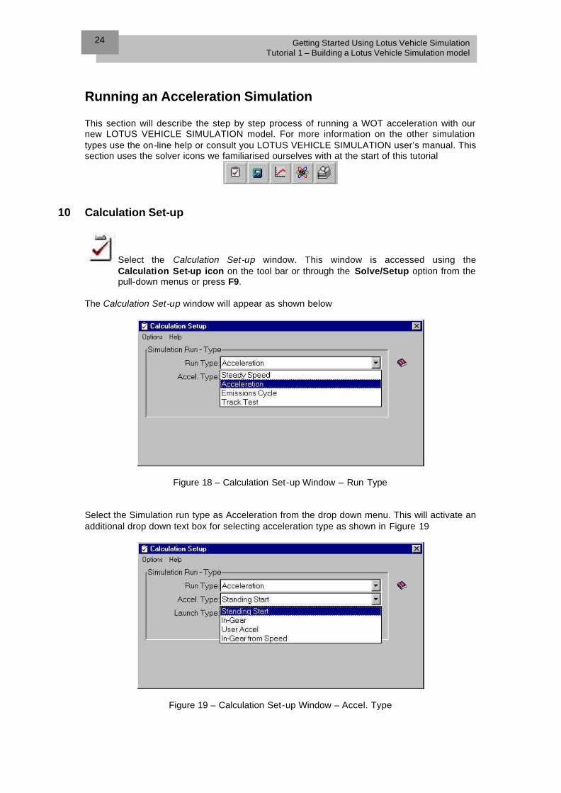
Running an Acceleration Simulation This section will describe the step by step process of running a WOT acceleration with our new LOTUS VEHICLE SIMULATION model. For more information on the other simulation types use the on-line help or consult you LOTUS VEHICLE SIMULATION user’s manual. This section uses the solver icons we familiarised ourselves with at the start of this tutorial

10 Calculation Set-up

Select the Calculation Set-up window. This window is accessed using the Calculation Set-up icon on the tool bar or through the Solve/Setup option from the pull-down menus or press F9.

The Calculation Set-up window will appear as shown below

Figure 18 – Calculation Set-up Window – Run Type

Select the Simulation run type as Acceleration from the drop down menu. This will activate an additional drop down text box for selecting acceleration type as shown in Figure 19

Figure 19 – Calculation Set-up Window – Accel. Type


25

Select the Acceleration type as Standing Start from the drop down menu. This will activate an additional drop down text box for selecting acceleration launch type as shown in Figure 20

Figure 20 – Calculation Set-up Window – Launch Type

Select the Launch type as Slip Start from the drop down menu.

The shift schedule panel at the bottom of the Calculation Set-up Window is used to scroll through the gear shift schedules using the arrow buttons. As no shift schedule was defined in the Gearbox data module for this example, the default shift schedule will be used

• Default Shift Scedule The default shift map is purely based on engine rpm and tractive effort, in that gear shift points are based on either the rpm limits of the engine, or the ability of a particular gear to give the greatest acceleration level. You have now defined the Simulation Run and its time to run the calculations.

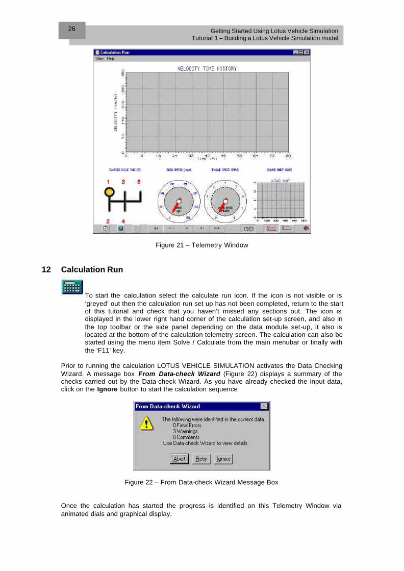
11 Telemetry Window

Select the Telemetry window. This window is accessed using the Solve Display icon on the tool bar or through the Solve/Display option from the pull-down menus or press F11.This will open the Telemetry window as shown in Figure 21. The Telemetry window is used to graphically show, engine speed, gear, vehicle speed, the test cycle and the engine load map via animation, as they vary throughout the simulation run

i


26

Figure 21 – Telemetry Window

12 Calculation Run

To start the calculation select the calculate run icon. If the icon is not visible or is ‘greyed’ out then the calculation run set up has not been completed, return to the start of this tutorial and check that you haven’t missed any sections out. The icon is displayed in the lower right hand corner of the calculation set-up screen, and also in the top toolbar or the side panel depending on the data module set-up, it also is located at the bottom of the calculation telemetry screen. The calculation can also be started using the menu item Solve / Calculate from the main menubar or finally with the ‘F11’ key.

Prior to running the calculation LOTUS VEHICLE SIMULATION activates the Data Checking Wizard. A message box From Data-check Wizard (Figure 22) displays a summary of the checks carried out by the Data-check Wizard. As you have already checked the input data, click on the Ignore button to start the calculation sequence

Figure 22 – From Data-check Wizard Message Box

Once the calculation has started the progress is identified on this Telemetry Window via animated dials and graphical display.


27

Displaying the Simulation Results This section will describe a method of displaying our simulation results. For more information on the other type of result interrogation use the on-line help or consult you LOTUS VEHICLE SIMULATION user’s manual. This section uses the results module icons we familiarised ourselves with at the start of this tutorial

When Lotus Vehicle Simulation calculations are performed it creates a number of results files, the extensions of which identify the type of results file it is.

Text results files have the form *_n.crs Graphical results files have the form *_n.grs Time history results files have the form *_n.vrs Where; n is the Plot File Counter number which is incremented for each calculation, and the ‘*’ is the Test No. string which you entered in the Vehicle Data window at the start of this tutorial.

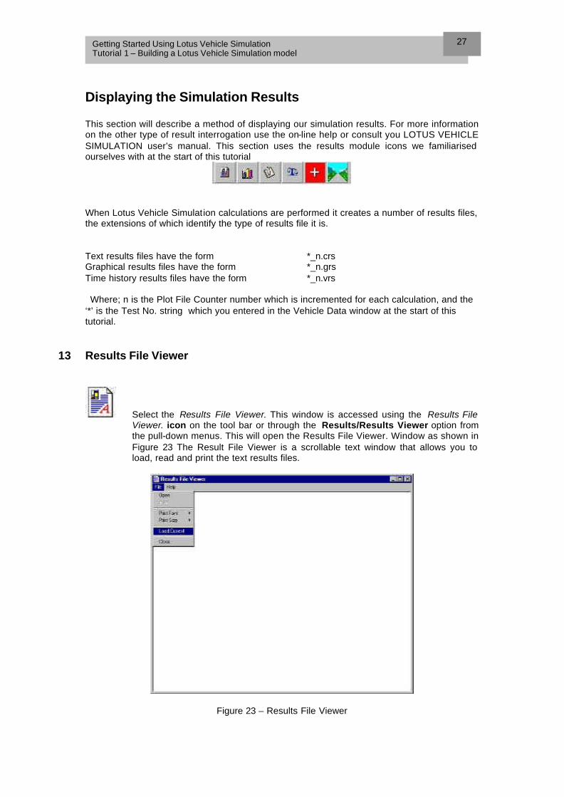
13 Results File Viewer

Select the Results File Viewer. This window is accessed using the Results File Viewer. icon on the tool bar or through the Results/Results Viewer option from the pull-down menus. This will open the Results File Viewer. Window as shown in Figure 23 The Result File Viewer is a scrollable text window that allows you to load, read and print the text results files.

Figure 23 – Results File Viewer


28

When a LOTUS VEHICLE SIMULATION solution is performed the result files are automatically written but they are not loaded into the viewer. To view the text results select the file option from Results File Viewer menu and select Load Current, as shown in Figure 23

Figure 24 – Results File Viewer – Load Current

Use this file to identify the 0-60 mph acceleration time of out example file (9.76 seconds)


29

To summaries what you have learnt from this tutorial • You have learnt how to start LOTUS VEHICLE SIMULATION

• You have familiarised yourself with LOTUS VEHICLE

SIMULATION

• You have inputted an example vehicle into LOTUS VEHICLE SIMULATION using the Data Modules

• You have used the Data Checking Wizard to check the validity of this input data

• You have run a Wide Open Throttle Acceleration simulation for this example vehicle

• You have loaded the simulation results into the Results file viewer and identified the 0-60 time for the example vehicle

This completes Tutorial 1 - Building a LOTUS VEHICLE SIMULATION Model


30

Tutorial 2 – Steady Speed Solver Application 3

Overview This tutorial takes you through an example model file and uses the steady speed solver option to evaluate the fuel economy impact of an engine coupled air conditioning unit This chapter includes the following sections: n Opening an example *.car file, 32

n View Selected Data Modules, 33

n Running the steady speed solver, 38

n Displaying the simulation results via:, 39

- Results Text File Viewer

n Analysing the simulation results, 40

n An Alternative analysis Method – Batch Analysis, 41

This Tutorial takes approximately ½ hour to complete

Getting Started Using Lotus Vehicle Simulation Tutorial 2 – Steady Speed Solver Application

32

Opening an example *.car file For this tutorial we will be using a predefined *.car file for a 1.5 litre 4 door saloon fitted with an automatic transmission, [filename: tutorial2.car ] Start LOTUS VEHICLE SIMULATION in the windows environment as previously described in Tutorial 1. Within the Startup Wizard select the Lotus Vehicle Simulation and Open an Existing .car file options before selecting OK to continue This displays the Open Existing file window as shown in Figure 25

Figure 25 – Open Existing File Window

Select the tutorial2.car option from the \\lesoft\examples directory and click OK. This opens the main Lotus Vehicle Simulation window,

Figure 26 – Lotus Vehicle Simulation Main Window


33

View Selected Data Modules The data module icons on the left hand side of the main window now contain all the information on the example vehicle. Click on these in turn to view this data

The following Data Module options contain data that is particularly interesting

Dyno Data

This window is accessed using the Dyno icon on the tool bar or through the Data/Dynamometer option from the pull-down menus. The section is concerned with the load vs. vehicle speed relationship applied by a chassis dynamometer for a vehicle running on this type of test-bed. Selecting Dyno data displays the Dyno Data window as shown in Figure 27

Figure 27 – Dyno Data Window

Driveline Data

This window is accessed using the Driveline icon on the tool bar or through the Data/Driveline option from the pull-down menus or press F4. This action will call into view the driveline sub-menu, which provides access to the various driveline data-windows.

Selecting TC/Clutch from the Driveline sub-menu, this will display the Drivetrain couple window shown in Figure 28


34

Figure 28 – Driveline Couple Window We have already investigated this window in Tutorial 1, but this time the option drop down list box shows that the torque converter option has been selected. This option activates the spreadsheet on the right hand side of the window, which contains the data required to model the torque converter.

For more information on the format of the torque converter data, use the on-line help . For the theory associated with this data module investigate the theory section of the on-line help

Selecting TC Lock-up from the Driveline sub-menu, will display the Torque Converter Lock-up window shown in Figure 29

Figure 29 – Torque Converter Lock-up Window Modern automatic transmission typically employ some form of torque converter lock-up strategy to improve efficiency.The lock-up strategy is defined as a set of lock-on and lock-off points defined in terms of any map variable vs. speed (Various speed variables are available) for a range or load fractions (up to 10). This data is shown in the spreadsheet on the right hand side of the Torque Converter Lock-up Window,


35

Selecting TC Idle from the Driveline sub-menu, will display the Torque Converter Idle window shown in Figure 30.

Figure 30 – Torque Converter Idle Speed Window The Torque Converter Idle Speed window is used to set the torque idle strategy. This is concerned with the operation of the Torque Converter during periods of zero power transmission. There are three options accessed using the ‘Idle Mode’ pop-down menu in the window. For the example file being used in this tutorial Normal Idle has been selected. In Normal idle mode the gearbox remains in drive and the window shows the attributed engine parameters for this condition.

Gearbox Data

Select the Gearbox menu. To enter or review data for the gearbox, select the Gearbox Icon from the icon panel. Alternatively, select Data / Gearbox from the main window menu bar or press F5.

Select Shift Strategy from the Gearbox sub-menu, this will display the gearbox shift strategy window shown below.

Figure 31 – Gear Shift Strategy Window


36

In tutorial 1 a default shift strategy was used. To mimic gearbox shift operations a shift strategy map is entered as an array of change up and change down data for each gear ratio across a 2-D map of a speed variable vs. a load variable.

• Displaying the Shift Strategy graphically The shift strategy can be displayed graphically using the graph icon at the top right of the window. Try the zoom, autoscaling, data pick and printing features accessed from the pull-down menu at the top left of the graphics window.

Figure 32 – Gear Shift Strategy Graphics Window

Engine Data


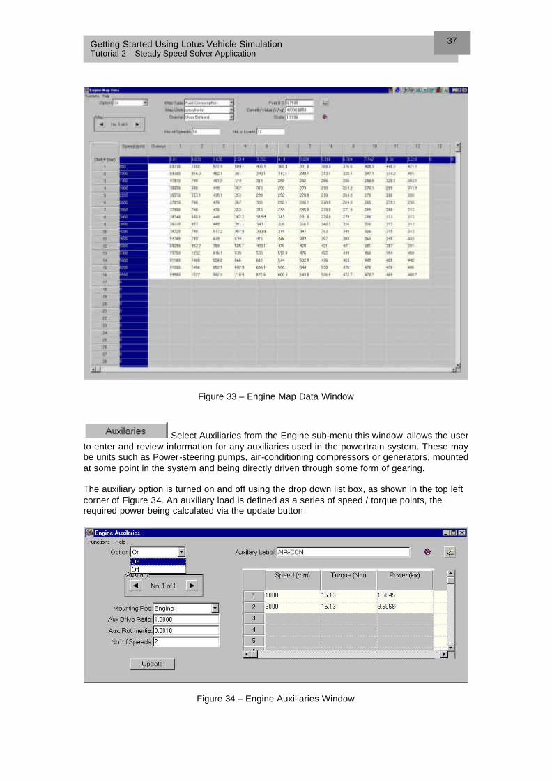
Select Map Data from the Engine sub-menu, this will display the engine map data window shown in Figure 33 This window is designed to permit easy entry of data for the engine fuel economy, emissions and operating characteristics over the load-speed range. The data shown in Figure 33 is a engine speed / BMEP map of fuel consumption data, with units of grams/kWhr. For more information on engine maps consult the on-line help, via the Help icon or using the relevant menu option

i


37

Figure 33 – Engine Map Data Window

Select Auxiliaries from the Engine sub-menu this window allows the user to enter and review information for any auxiliaries used in the powertrain system. These may be units such as Power-steering pumps, air-conditioning compressors or generators, mounted at some point in the system and being directly driven through some form of gearing. The auxiliary option is turned on and off using the drop down list box, as shown in the top left corner of Figure 34. An auxiliary load is defined as a series of speed / torque points, the required power being calculated via the update button

Figure 34 – Engine Auxiliaries Window


38

Running the Steady Speed Solve This tutorial has been designed to demonstrate the influence of an auxiliary load on engine fuel consumption. This influence is quantified using the steady speed solver option and the Auxiliaries Engine sub-menu option Generate the required data using the following 12 point test matrix Vehicle Speed 10, 40, 60, 80, 100, 140 km/hr Air Conditioning Auxiliary unit ON Vehicle Speed 10, 40, 60, 80, 100, 140 km/hr Air Conditioning Auxiliary unit OFF

Calculation Set-up


The Calculation Set-up window will appear as shown in Figure 35 select the steady speed solver, with a shift option of Set Shift Schedule and Speed. Then select speed units of km/hr and enter the first speed value of 10 km/hr

Figure 35 – Calculation Set-up Window The shift schedule panel at the bottom of the Calculation Set-up Window is used to scroll through the gear shift schedules using the arrow buttons. The shift schedule defined in the Gearbox data module for this example, is Econ-Map. Ensure the AIR_CON auxiliary is switched on in the Auxiliaries - Engine sub-menu

To start the calculation select the calculate run icon, ignoring any data checking comments or warnings. Unlike tutorial 1, the telemetry screen is not opened so as to increase simulation speed

• This is run 1 of 12


39

Displaying the Simulation Results To obtain the fuel consumption data for this simulation run use the Results File Viewer as in Tutorial 1

Results File Viewer

Select the Results File Viewer. This window is accessed using the Results File Viewer. icon on the tool bar or through the Results/Results Viewer option from the pull-down menus. This will open the Results File Viewer. Window as shown in Figure 36. Load the current results and scroll down to the bottom of the file

Figure 36 – Results File Viewer Window Read off the Fuel Consumption from Map… 1, Litres per 100km value

17.399 l/100km


40

Analysing the simulation results Repeat this simulation for all 12 point of the test matrix – completing the tables below. The Air CON auxiliary is turned off via the Auxiliaries - Engine sub-menu

Fuel Consumption [litres/100km]

Vehicle Speed

Air Con ON Air Con OFF

10 km/hr

40 km/hr

60 km/hr

80 km/hr

100 km/hr

140 km/hr

Plotting these values, shows a 20% increase in fuel consumption, across the vehicle speed range for operation with air conditioning on.


41

An Alternative Analysis Method – Batch Analysis To solve the 12 point test matrix requires 12 individual steady speed simulation runs. The following approach uses one of the built-in LOTUS VEHICLE SIMULATION tools to produce a BATCH Simulation, to speed up analysis time

The batch analysis option allows the user to define a series of different tests that can be run in one go without the need to redefine the test settings between tests. The results can be selected from either the '.crs' file variables or the '.grs' file variables. The grs results can further be requested at either the end of the cycle, at a user selected time, a user selected distance or a user selected velocity during the cycle. A number of different results can also be defined for each test case. The results are listed into a scrollable text widget, the contents of which can be printed or saved to a file. The solution settings for each batch test are defined using the normal style calculation setting buttons, the displayed settings being updated for each test as you step through the tests.

Using the Batch Analysis tool requires only two batch simulations to complete the test matrix, one with the air conditioning turned ON and another with the air conditioning turned ON

i


42

To summaries what you have learnt from this tutorial n You have investigated some additional data modules

within the example *.car file

n You have run a test matrix of steady speed solver runs, viewing the results via the Results Text Viewer.

n You have analysed these results to access the impact of an air conditioning unit power requirements on fuel economy

n You have used an alternative analysis method – Batch Analysis

This completes Tutorial 2 – Steady Speed Solver Application

Tutorial 3 – Acceleration Solver Application

4

Overview This tutorial takes you through two example model files and uses the acceleration solver option to evaluate the improvement in acceleration performance when turbo-charging an example naturally aspirated vehicle. This chapter includes the following sections: n Opening an example *.car file, 43

n Running the Acceleration Solver, 45

n Calculation Set-up, 45

n Display the Simulation Results, 46

n An Extension to the Batch Analysis Approach, 48

This Tutorial takes approximately ½ hour to complete

Getting Started Using Lotus Vehicle Simulation Tutorial 3 – Acceleration Solver Application

44

Opening an example *.car file For this tutorial we will be using a predefined *.car file for a 1.6 litre 2 door sports car fitted with a manual transmission, [filename: tutorial3a.car ].We will also later use the turbo-charged variant of the same vehicle, [filename: tutorial3t.car ]. Start Lotus Vehicle Simulation in the windows environment as previously described in Tutorial 1. Within the Startup Wizard select the Lotus Vehicle Simulation and Open an Existing .car file options before selecting OK to continue This displays the Open Existing file window as shown in 37

Figure 37 – Open Existing File Window

Select the tutorial3a.car option from the \lesoft\examples directory and click OK. This opens the main Lotus Vehicle Simulation window. As in the previous tutorial the individual data icons can be used to view the data associated with each Data Module. For this tutorial the data we are most interested in is the engine data.

Engine Data


Select Engine from the Engine sub-menu, this will display the engine data window, as shown in Figure 38, which is used to review or adjust engine data.

This shows for the N.A. version a peak BMEP value of 10.75 bar at 4600 rpm.

The notepad editor icon on this display can be used to view the engine data in a number of different units. This can be useful for entering engine performance data in units other BMEP or Torque. If this approach is taken then the ‘file / close save changes’ option should be used.


45

Figure 38 Engine Data – N.A. derivative

Running the Acceleration Solver This tutorial has been designed to demonstrate the influence of engine power on overall vehicle performance. In a similar way to the previous tutorial we will run a number of simulations to complete a matrix of results for the two engine variants. The required results are; 0-60 mph, 0-100 mph, 0-100 kmh, Vmax (at tolerance), time to ¼ mile , 40-50 mph in 3rd gear and 90-100 mph in 4th gear.

Calculation Set-up


The Calculation Set -up window will appear as shown below select the acceleration speed solver, with an Accel. Type of ‘Standing start’ and a Launch Type of ‘Slip Start’. Set the Shift Schedule option to ‘Default Shift Schedule’.


46

Start the calculation using the ‘calculate run icon’, this run will provide us the answers to the first five results.

Displaying the Simulation Results To obtain the acceleration data for this simulation run use the Results File Viewer as in Tutorial 1

Results File Viewer

Select the Results File Viewer. This window is accessed using the Results File Viewer. icon on the tool bar or through the Results/Results Viewer option from the pull-down menus. This will open the Results File Viewer. Window as shown in Figure 39. Load the current results and scroll down to the bottom of the file.

Figure 39 – Acceleration Results, NA variant Read off the acceleration times;

0-60 mph 8.354 s 0-100 mph 25.959 s 0-100 kmh 8.842 s

¼ mile 16.556 s Vmax (at tol) 118.37 mph


47

Go back to the Calculation Set -up window and change the acceleration type to be ‘In-Gear’, Select gear number 3 and re-run the analysis. In the same way as above extract the required result for 40 – 50 mph in 3rd gear, in this case 2.8206 s. Repeat the previous in-gear analysis for 4th gear and extract the required result, 90 – 100 mph in 4th gear. The results can now be entered into the table below for the NA variant.

Acceleration Time (s) or Speed (mph)

Acceleration

Result N.A.

(tutorial3a.car)

Turbo

(tutorial3t.car)

0 – 60 mph

0 – 100 mph

0 – 100 kmh

¼ mile

Vmax (at tol) (mph)

40 – 50 mph in 3rd gear

90 – 100 mph in 4th Gear

Now load the turbocharged model variant, tutorial3t.car. Use the data Icons to review the engine data. Note that this model has a peak BMEP figure of 15.77 bar and a maximum power of 165 bhp compared to the peak power of 121 bhp for the NA variant. You will also notice a number of other changes between the two models, the most relevant of which is the maximum engine speed was dropped to 7000 rpm for the turbocharged engine. You will have noticed that the Vmax results are given for both the end of the run and at the acceleration tolerance point. This was introduced for two reasons, firstly it clearly identifies whether a vehicle has achieved its maximum velocity within the defined cycle time, (default length 80 seconds for an acceleration run but can be reset via the calculation set-up window under the menu option ‘Options / Settings’), and secondly it allows a method of defining time to Vmax. The tolerance used for identifying Vmax can be changed by the user in the same way as identified for the run time above.


48

Repeat the three analysis runs previously performed for the NA variant with the new turbocharged model, record the answers and complete the table. The chart below summarises the results, and highlights the reductions in acceleration times of up to 33% achieved with the increased engine performance.

An Extension to the Batch Analysis Approach Again as identified in the previous tutorial the Batch analysis approach could be used to perform the required analysis in one job submission per vehicle. Users need to be aware that the setup for batch runs are stored in the users ini file, thus next time the application is started the previous settings for the batch runs are restored. Hence the ini file can be used as a means of storing/retrieving different batch set-ups by using the menu options ‘file / save ini file’ and ‘file / load ini file’.

0

5

10

15

20

25

30

$1.00 $2.00 $3.00 $4.00 $5.00 $6.00

Run Type

Tim

e (s

)

N.A. Turbo

0-600 mph 0-100 mph 0-100 kmh ¼ mile 40-50 mph 3rd 90-100 mph 4th

i


49

To summaries what you have learnt from this tutorial n You have investigated some of the alternative

acceleration solver options

n You have run a test matrix of acceleration solver runs, viewing the results via the Results Text Viewer.

n You have analysed these results to access the impact of engine performance on overall vehicle performance.

This completes Tutorial 3 – Acceleration Solver Application


50

Tutorial 4 – Emissions Cycle Solver Application 5

Overview This tutorial takes you through an example model file and uses the cycle solver option to evaluate the improvement in tail pipe emissions achieved with the addition of a chosen catalyst. This chapter includes the following sections: n Opening an example *.car file, 52

n Running the Emissions Cycle Solver, 54



n X-Y Results Plotting, 56

n Use of the Parametric Analysis Tool, 58

This Tutorial takes approximately 3/4 hour to complete

Getting Started Using Lotus Vehicle Simulation Tutorial 4 – Emissions Cycle Solver Application

52

Opening an example *.car file For this tutorial we will be using a predefined *.car file for a 1.6 litre low emissions example vehicle fitted with a manual transmission, [filename: lev.car ]. Start Lotus Vehicle Simulation in the windows environment as previously described in Tutorial 1. Within the Startup Wizard select the Lotus Vehicle Simulation and Open an Existing .car file options before selecting OK to continue This displays the Open Existing file window as shown below

Select the tutorial4.car option with the \\lesoft directory and click OK. This opens the main Lotus Vehicle Simulation window. As in the previous tutorial the individual data icons can be used to view the data associated with each Data Module. For this tutorial the data we are most interested in is the engine data.

Engine Data


Select Map Data from the Engine sub-menu, this will display the engine map data window, as shown below, which is used to review or adjust the map data.


53

Screen Shot of Map Data

The data can also be viewed as a series of contour plots using the graph icon.

Example HC Emissions Map

This model already has a catalyst included in it. You should review the data associated with this component and the technique employed to define the individual overall efficiencies for HC Nox and CO as well as the warm-up characteristics for each.


54

Catalyst Modelling Data

Running the Emission Cycle Solver This tutorial has been designed to demonstrate the influence of a catalyst on overall vehicle emissions, with particular reference to the warm-up portion of an emissions cycle. We will run two basic vehicle specifications to assess the reductiyon in emissions levels due to the addition of a catalyst and then additional runs to review the impact of changing the catalyst warm-up properties on total emissions. The required results are; Hydrocarbon Emissions (g), Nox Emissions (g), CO Emissions (g). Both with and without the catalyst.

Calculation Set-up


The Calculation Set-up window will appear as shown below, set the run type as ‘Emissions Cycle’, with an Origin. Type of ‘USA’ and a Test Name of ‘Federal FTP 75 Drive Cycle’. Users who are not familiar with the nature of this cycle should run the program with the telemetry screen displayed to see the nature of the cycles velocity time history.


55

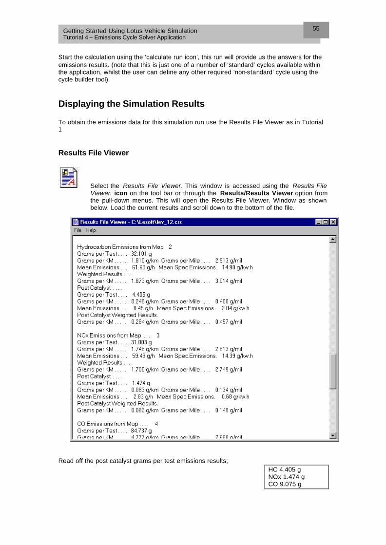
Start the calculation using the ‘calculate run icon’, this run will provide us the answers for the emissions results. (note that this is just one of a number of ‘standard’ cycles available within the application, whilst the user can define any other required ‘non-standard’ cycle using the cycle builder tool).

Displaying the Simulation Results To obtain the emissions data for this simulation run use the Results File Viewer as in Tutorial 1

Results File Viewer

Select the Results File Viewer. This window is accessed using the Results File Viewer. icon on the tool bar or through the Results/Results Viewer option from the pull-down menus. This will open the Results File Viewer. Window as shown below. Load the current results and scroll down to the bottom of the file.

Read off the post catalyst grams per test emissions results;

HC 4.405 g NOx 1.474 g CO 9.075 g


56

To get the results for a model without a catalyst we could either go to the ‘Catalyst’ data section under the engine module and set the option to ‘off’. Alternatively if we examine our existing results listed above the post catalyst results are the pre-catalyst values. Thus we can simply extract the results from the same file; Read off the pre catalyst grams per test emissions results;

HC 32.101 g NOx 31.003 g CO 84.737 g

X-Y Results Plotting Before reviewing the impact of catalyst properties on post catalyst emissions we will look at ways of cross plotting cycle varying properties. These values are stored in the ‘grs’ file created during each run, this file is different to the ‘crs’ file that is displayed in the text viewer which contains cycle averaged values.

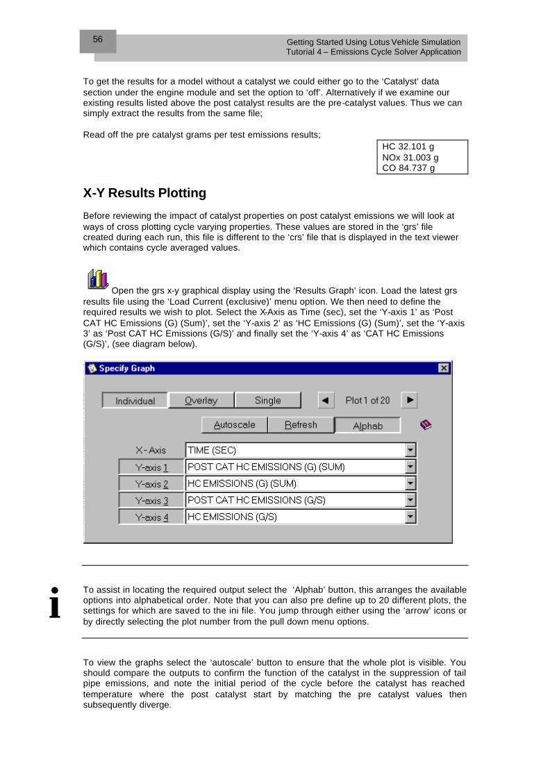
Open the grs x-y graphical display using the ‘Results Graph’ icon. Load the latest grs results file using the ‘Load Current (exclusive)’ menu option. We then need to define the required results we wish to plot. Select the X-Axis as Time (sec), set the ‘Y-axis 1’ as ‘Post CAT HC Emissions (G) (Sum)’, set the ‘Y-axis 2’ as ‘HC Emissions (G) (Sum)’, set the ‘Y-axis 3’ as ‘Post CAT HC Emissions (G/S)’ and finally set the ‘Y-axis 4’ as ‘CAT HC Emissions (G/S)’, (see diagram below).

To assist in locating the required output select the ‘Alphab’ button, this arranges the available options into alphabetical order. Note that you can also pre define up to 20 different plots, the settings for which are saved to the ini file. You jump through either using the ‘arrow’ icons or by directly selecting the plot number from the pull down menu options.

To view the graphs select the ‘autoscale’ button to ensure that the whole plot is visible. You should compare the outputs to confirm the function of the catalyst in the suppression of tail pipe emissions, and note the initial period of the cycle before the catalyst has reached temperature where the post catalyst start by matching the pre catalyst values then subsequently diverge.

i


57

Results Graph for HC Emissions To assess the impact of the catalyst properties on the overall emissions performance complete the table below, re-running the analysis with different properties as identified in the table.

Parameter HC Emissions g/test No/Pre Catalyst 32.101 Std Data 4.405 HC Max Effy = 0.90 HC Max Effy = 0.85 HC Max Effy = 0.80 HC Max Effy = 0.75 Revert to Std Data 4.405 HC Time to Max Effy (s) = 160 HC Time to Max Effy (s) = 140 HC Time to Max Effy (s) = 120 HC Time to Max Effy (s) = 80 Revert to Std Data 4.405 HC Warming Time (s) = 30 HC Warming Time (s) = 35 HC Warming Time (s) = 40


58

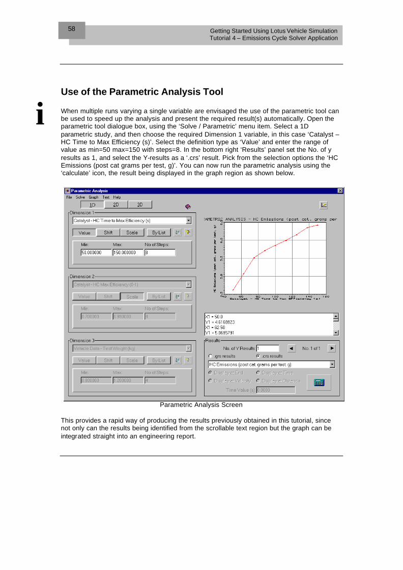
Use of the Parametric Analysis Tool When multiple runs varying a single variable are envisaged the use of the parametric tool can be used to speed up the analysis and present the required result(s) automatically. Open the parametric tool dialogue box, using the ‘Solve / Parametric’ menu item. Select a 1D parametric study, and then choose the required Dimension 1 variable, in this case ‘Catalyst – HC Time to Max Efficiency (s)’. Select the definition type as ‘Value’ and enter the range of value as min=50 max=150 with steps=8. In the bottom right ‘Results’ panel set the No. of y results as 1, and select the Y-results as a ‘.crs’ result. Pick from the selection options the ‘HC Emissions (post cat grams per test, g)’. You can now run the parametric analysis using the ‘calculate’ icon, the result being displayed in the graph region as shown below.

Parametric Analysis Screen This provides a rapid way of producing the results previously obtained in this tutorial, since not only can the results being identified from the scrollable text region but the graph can be integrated straight into an engineering report.

i


59

To summaries what you have learnt from this tutorial n You have investigated how to perform an emission

cycle analysis

n You have reviewed the impact of catalyst properties on solution output.

n You have used the parametric analysis tool to rapidly

review data variable change.

This completes Tutorial 4 – Emission Cycle Solver Application


60

Tutorial 5 – Track Solver Application

6

Overview This tutorial takes you through an example model file and uses the track solver option to evaluate the effect on lap times of varying the final drive ratio. This chapter includes the following sections: n Opening an example *.car file, 62

n Running the Track Solver, 63



n 3D Viewing of the Results, 65

n Use of the DataBase Tool, 66

n Use of the Parametric Analysis Tool for Multi-Variant

analysis, 68

This Tutorial takes approximately 1/2 hour to complete

Getting Started Using Lotus Vehicle Simulation Tutorial 5 – Track Solver Application

62

Opening an example *.car file For this tutorial we will be using a predefined *.car file for a 2.2 litre turbocharged high performance sports car, fitted with a manual transmission, [filename: tutorial5.car ]. Start Lotus Vehicle Simulation in the Windows environment as previously described in Tutorial 1. Within the Startup Wizard select the Lotus Vehicle Simulation and Open an Existing .car file options before selecting OK to continue This displays the Open Existing file window as shown below

Select the tutorial5.car option with the \\lesoft directory and click OK. This opens the main Lotus Vehicle Simulation window. As in the previous tutorial the individual data icons can be used to view the data associated with each Data Module. For this tutorial the data we are most interested in is the driveline data.

Final Drive Data

Select the Driveline data -menu. To enter or review data for the driveline, select the

Driveline Icon from the icon panel. Alternatively, select Data / Driveline from the main window menu bar or press F4.

Select Final Drive from the Driveline sub-menu, this will display the final drive data window, as shown below, which is used to review or adjust the final drive data.


63

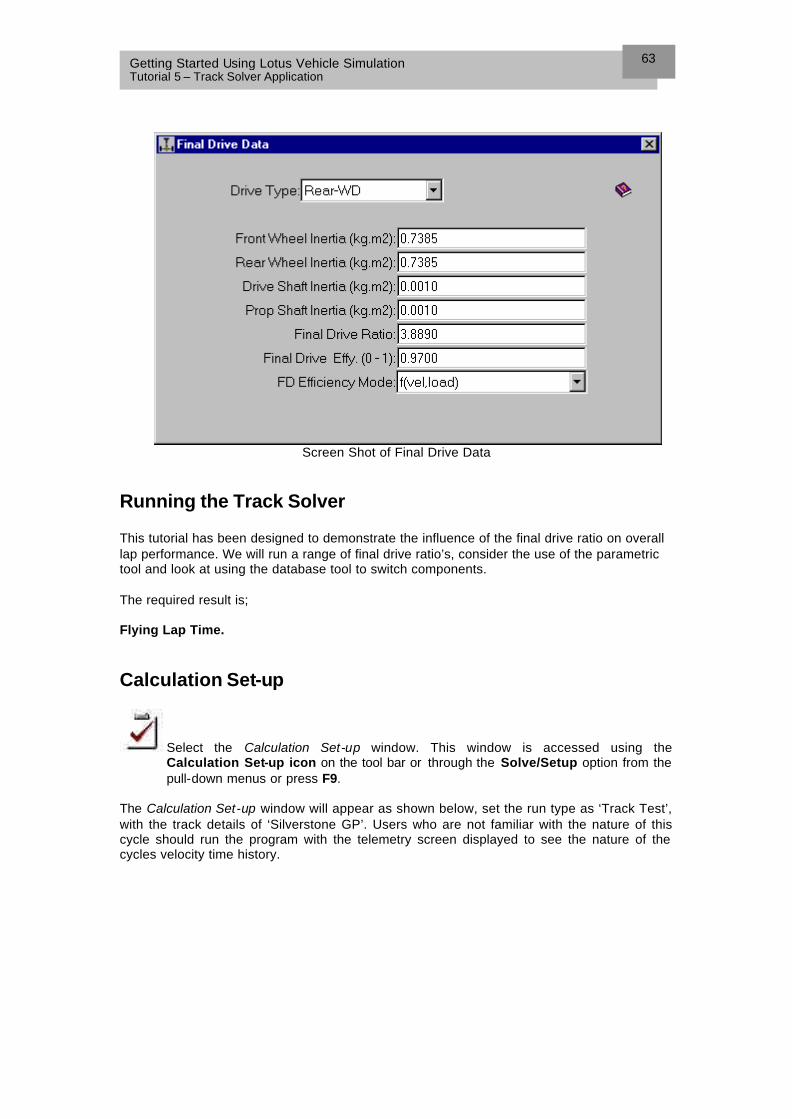
Screen Shot of Final Drive Data

Running the Track Solver This tutorial has been designed to demonstrate the influence of the final drive ratio on overall lap performance. We will run a range of final drive ratio’s, consider the use of the parametric tool and look at using the database tool to switch components. The required result is; Flying Lap Time.

Calculation Set-up


The Calculation Set-up window will appear as shown below, set the run type as ‘Track Test’, with the track details of ‘Silverstone GP’. Users who are not familiar with the nature of this cycle should run the program with the telemetry screen displayed to see the nature of the cycles velocity time history.


64

Track Solver Set-up Start the calculation using the ‘calculate run icon’, this run will provide us the answer for the lap times. (note that this is just one of a number of ‘standard’ tracks available within the application, whilst the user can define any other required ‘non-standard’ tracks using the track builder tool).

Displaying the Simulation Results To obtain the flying lap time data for this simulation run use the Results File Viewer as in the previous tutorials.

Results File Viewer

Select the Results File Viewer. This window is accessed using the Results File Viewer. icon on the tool bar or through the Results/Results Viewer option from the pull-down menus. This will open the Results File Viewer. Window as shown below. Load the current results and scroll down to the bottom of the file.

Results Viewer


65

Read off the flying lap time result;

Lap Time (flying lap) 168.233 s Now modify the final drive ratio and rerun the analysis to complete the Table below.

Final Drive Ratio Lap Time 3.889 168.233

4.5 4.4 4.3 4.2 4.1 4.0 3.8 3.7 3.6 3.5

3D Viewing of the Results The track analysis results can be viewed through the 3D display. This shows not only an image of the driving event, but also a number of key simulation results such as speed, gear, lateral/longitudinal acceleration and time.

Open the 3D viewer using the ‘3D Viewer’ icon. Load the latest grs results file using the ‘Load Current (exclusive)’ menu option. You can then set the visibility of the various display elements via the visibility menu, (see example below).

3D Track Results Viewer


66

Use of the DataBase Tool One way of reviewing model changes is to change the data in a model by editing a single value. This tutorial is an example of that where we have incrementally changed the final drive ratio between analysis runs. An alternative approach is to think in terms of complete components. A final drive component has a collection of properties, not just the final drive ratio, such that when considering changes to final drive ratio we could replace the properties for the complete component. The DataBase tool is a mechanism that can be used to switch component data around, to demonstrate the use of the DataBase tool we will swap the existing Final Drive with one stored in the example DataBase provided with the install. Open the DataBase tool using the menu ‘Tools / DataBase Wizard’. Open the example database using the menu option ‘DataBase / Open (exclusive)’, and browse for ‘example.dbs’. The database tool list data by component. The components are grouped under ‘compulsory’, ‘optional’ and ‘controllers’. In the compulsory group select the final drive ratio icon (shown below)

Selected Final Drive Icon

Once the final drive ratio icon is selected, the two entries stored will be shown in the Component List, (see display below)

DataBase Tool display Select the top entry ‘Example final drive’ and press ‘Add’, the display will change to show the ‘Drive’ icon on the display without the coloured bar, this indicates that data has been loaded for this component. To view the component properties, either select the ‘properties’ button or use the right mouse button menu on the ‘Drive’ icon. The properties dialogue box is shown below.


67

Properties Display

To get this new final drive component copied into the model select the ‘File / Make Current’ option. This will copy over to your existing model any selected component changes, (in our case just the final drive changes). Now select the ‘File / Close’ option, (ignore the warning message). Selecting the driveline data box will now show for the final drive component the properties of the new component.

New Component Properties With this new component the flying lap time is now; Read off the flying lap time result;

Lap Time (flying lap) 167.902 s


68

Use of the Parametric Analysis Tool for Multi-Variant Analysis The parametric tool could have been used again in this tutorial to run the final drive ratio analysis as a 1D parametric run. We could extend the parametric tool use to 2 or 3 data variant analysis tasks. We could review the impact on lap times of variations in 3rd 4th and 5th gear ratios. Select a 3D parametric option and select the variables to be ‘Gearbox Data –Ratio Gear 5’, ‘Gearbox Data –Ratio Gear 4’ and ‘Gearbox Data –Ratio Gear 3’. Select the one required Y-result to be ‘Lap Time – Flying lap (s)’. Set all parameters to be ‘By Scale’ and set values as min=0.8, max=1.2 with 5 steps.

Parametric Analysis Screen

This provides a rapid way of assessing the overall impact on lap times for the three interrelated gear ratio’s. The scrolled display can be used to find the quickest lap time. The quickest flying lap time was;

Lap Time (flying lap) 167.887s

i


69

To summaries what you have learnt from this tutorial n You have investigated how to perform a track analysis

n You have used the database tool to exchange

complete component data, rather than editing a single value.

n You have used the parametric analysis tool to rapidly

review multi-variant data change.

This completes Tutorial 5 – Track Solver Application