Embed Size (px)
Citation preview
G E T T I N G S T A R T E D US ING L O T U S C O N C E P T V A L V E T R A I N
V E R S I O N 2 . 0 5

The information in this document is furnished for informational use only, may be revised from time to time, and should not be construed as a commitment by Lotus Cars Ltd or any associated or subsidiary company. Lotus Cars Ltd assumes no responsibility or liability for any errors or inaccuracies that may appear in this document. This document contains proprietary and copyrighted information. Lotus Cars Ltd permits licensees of Lotus Cars Ltd software products to print out or copy this document or portions thereof solely for internal use in connection with the licensed software. No part of this document may be copied for any other purpose or distributed or translated into any other language without the prior written permission of Lotus Cars Ltd. ©2001 by Lotus Cars Ltd. All rights reserved.
Getting Started Using Lotus Concept Valve Train Contents
i
Contents About This Guide v Welcome to Lotus Concept Valve Train v What you Need to Know v Chapter 1. Introducing Lotus Concept Valve Train 1 Overview 1 What is Lotus Concept Valve Train? 2 Normal Uses of Lotus Concept Valve Train 3 Overall Concepts 4 About the Tutorials 5 Getting Help Online 6 Chapter 2. Tutorial 1, ‘Getting Started’ 9 Overview 9 Starting Lotus Concept Valve Train 10 Familiarising Yourself with Lotus Concept Valve Train 11 Opening a Saved File 12 Direct Editing of Model Data 12 Viewing the Results Panel 13 Listing the Profile Incremental Results 13 The use of Report Warnings 14 Closing the Application 14 Chapter 3. Tutorial 2, ‘Reviewing Model Template Types’ 15 Overview 15 Selecting a New Template Type 16 Changing the Motion Type 17 Viewing the Profile Segments 17 Closing the Application 18 Chapter 4. Tutorial 3, ‘Modifying the Cam Profile’ 19 Overview 19 Direct Editing of Profile Points 20 The Concepts of ‘fix’ and ‘un-fix’ 21 Modifying a Profile Using Joggle 21 Chapter 5. Tutorial 4, ‘Modifying the Mechanism’ 23 Overview 23 Displaying the Mechanism Graphics 24 Direct Editing of the Mechanism 24 Editing of the Mechanism Through the Display 25 Application of Joggle to the Mechanism Geometry 26 Design Exercise 26
Getting Started Using Lotus Concept Valve Train Contents
ii
Chapter 6. Tutorial 5, ‘A Real Example’ 27 Overview 27 Reviewing supplied geometry, 28 Opening the application and loading required template, 28 Modifying the template geometry, 29 Assessing the lift limitations, 32 Chapter 7. Tutorial 6, ‘Reviewing Static’s Data’ 33 Overview 33 Static’s Data Variables 34 Spring cover 34 Hertzian Contact Stress 35 Design Exercise 35 Design Exercise Results 36 Chapter 8. Tutorial 7, ‘A Look at Valve to Piston Clearance’ 37 Overview 37 Piston Clearance Valve Lift Data Variables 38 Piston Clearance, Engine Geometry Data Variables 39 Piston Clearance, Valve Geometry Data Variables 39 Design Exercise 40 Design Exercise Result 41 Chapter 9. Tutorial 8, ‘Spring Design’ 43 Overview 43
Screen Layout 44 Graphical Options 44 Spring Design Data 45 Spring Design Options 46 Design Exercise 46 Application to Valve Train Static’s 47 Chapter 10. Tutorial 9, ‘Export of Data’ 49 Overview 49 Preparing for Export 50 Exporting the Cam Profile 50 Exporting the Sub-System Model 52 Exporting Directly from the Preview 52 Preparing to Run ADAMS/Engine 53 Running ADAMS/Engine 54 Chapter 11. Tutorial 10, ‘Import of Profile Data’ 55 Overview 55 Producing Profile Lift Data Files 56 Importing Lift Data 57 Using Smoothing and Clipping 58 Importing Full Profile Data 59 Uses of Profile Import 59
Getting Started Using Lotus Concept Valve Train About This Guide
iii
Chapter 12. Tutorial 11, ‘Migration Within Lotus Simulation Tools’ 61 Overview 61 Opening the Engine Simulation Component 62 Loading an Existing Engine Simulation File 63 Switching to Lotus Concept Valve Train 63 Making the Valve Lift Profile Current 64 Viewing the Changes 65 Further Data Exchange Opportunities 66 Chapter 13. Tutorial 12, ‘Using Bezier Acceleration Curves’ 67 Overview 67 Bezier Curves, an Overview 68 Generating a Symmetrical Bezier Based Cam Profile 69 Producing a Valid Symmetrical Bezier Cam Profile 71 Editing and Manipulating Bezier Points 73 Adding and Deleting Bezier Control Points 74 Generating an Asymmetric Bezier Profile 75 Producing a Valid Asymmetric Bezier Cam Profile 76 Chapter 14. Tutorial 13, ‘The Dynamic Spring Module’ 79 Overview 79 Dynamic Analysis, an Overview 80 Changing to the Dynamics Module 81 Dynamic Model Types 82 Auto-Creating the Complete Model 82 Auto-Updating Model Parts 83 Selecting and Editing Mass Properties 84 Selecting and Editing Link Properties 85 ‘Special’ Element Properties 86 Defining the Profile 87 Defining Gas Loads 87 Running the Analysis 88 Controlling the Results Screen Display 90 Listing Overall Results 92 Chapter 15. Tutorial 14, ‘The Concavity Tool’ 95 Overview 95 The Concavity Tool, an Overview 96 Opening the Concavity Tool 97 Loading the Cam Surface Data 98 Analysing the Cam Lobe 99 The ‘General Settings’ 100 Running the Auto Correction 101 Applying the Changes 101

Getting Started Using Lotus Concept Valve Train Contents
iv
Getting Started Using Lotus Concept Valve Train About This Guide
v
About This Guide Welcome to Lotus Concept Valve Train Welcome to Lotus Concept Valve Train. Using Lotus Concept Valve Train, you can design and review camshaft profiles, apply them to mechanism templates and analyse their quasi-static kinematic performance. Lotus Concept Valve Train also provides tools for valve spring design, valve to piston clearance studies and valve overlap calculations. What You Need to Know This guide assumes the following: n Lotus Concept Valve Train is installed on your computer or network and you have
permission to execute Lotus Concept Valve Train module.
n The necessary password files are installed to allow you to run the necessary modules.
n You have a basic understanding of valve train mechanisms and the relevance and limitations of camshaft profile properties.

Getting Started Using Lotus Concept Valve Train About This Guide
vi
Overview This chapter introduces you to Lotus Concept Valve Train and explains the normal uses for it. It also introduces the tutorials that we’ve included in this guide to get you started working with Lotus Concept Valve Train. This chapter contains the following sections:
n What is Lotus Concept Valve Train?, 2
n Normal Uses of Lotus Concept Valve Train, 3
n Overall Concepts, 4
n About the Tutorials, 5
n Getting Help Online, 6
1 Introducing Lotus Concept Valve Train
Getting Started Using Lotus Concept Valve Train Introducing Lotus Concept Valve Train
2
What is Lotus Concept Valve Train Lotus Concept Valve Train is an individual component in the Lotus Engineering simulation software environment. This component covers the design and analysis of valve train systems with particular reference to camshaft profiles, (often referred to as cam synthesis). It deals specifically with the concept phase using rigid body quasi-static analysis techniques. File export facilities are included to create models to use within the ADAMS/EngineTM simulation environment for in-depth dynamic analysis and virtual prototyping. Lotus Concept Valve Train has seven sections:
n Profile – Lets you define the camshaft profile mathematical function, using
segmented polynomials, the end and mid points of which you can define the values for in lift or any of the first three derivatives.
n Mechanism – Lets you define and graphically review the geometry for the
mechanism template currently selected. Includes x-y pivot co-ordinates, lengths and radii.
n Static’s – Lets you define the model data related to static analysis, and review
results graphs of the major calculated variables.
n Valve to Piston Clearance – Lets you study the effect on valve to piston clearance for the currently designed cam profile of valve timing and other related parameters.
n Spring Design – A tool to assist in the design and analysis of conventional round
wire valve springs of either linear of progressive rate. The designed spring loads can be applied directly to your cam design ‘static’s’ data section.
n Overlap – A tool to calculate the overlap area between two cam profiles given
the timing for the inlet and exhaust profiles.
n Dynamic Spring – A module for the analysis of a lumped mass multi-body representation of the valve train. The interactive display of the equivalent system animates the forced damped response during the analysis run.
Getting Started Using Lotus Concept Valve Train Introducing Lotus Concept Valve Train
3
Normal Uses of Lotus Concept Valve Train Lotus Concept Valve Train is used to assist in the design and analysis of camshaft profiles, valve springs and valve to piston clearance. In addition to the design of the cam lift function, the quasi-static analysis predicts forces, contact stress and float speeds for the defined system. As well as being applied to produce new cam profiles designs, the program can assess changes to an existing arrangement, review the suitability of an alternative existing camshaft profile with current system, design a new valve spring to suit a revised operating range and perform benchmarking of competitor camshafts.
Getting Started Using Lotus Concept Valve Train Introducing Lotus Concept Valve Train
4
Overall Concepts The structure of Lotus Concept Valve Train is based on a number of key concepts:
n Templates - A template approach is used in that cam mechanism types are provided as four basic types, Direct acting, centre-pivot rocker, finger follower and push rod rocker. Most conventional valve trains can be fitted into one of these broad classifications.
n Motion - The defined motion can be applied to either the valve end of the system
or the cam end of the system. n Polynomial - The motion function utilises segmented polynomials. Three default
polynomial types are provided to suit ‘standard applications’, ‘velocity limited’ and ‘acceleration limited’ cases. Within these polynomial ‘templates’ the user is then free to drag definition points around on lift and the first three derivatives or set polynomial exponents directly.
n Kinematic – The rigid body behaviour of the system under a prescribed motion at
a defined speed. Kinematic displacement and forces take no account of the elastic nature of the parts.
n Dynamic – The forced damped analysis of the equivalent lumped mass
representation of the system. The elastic behaviour of component parts allows separation of parts to be predicted.
Getting Started Using Lotus Concept Valve Train Introducing Lotus Concept Valve Train
5
About the Tutorials The remainder of this guide is structured around a series of tutorials that introduce you to the features of Lotus Concept Valve Train. Each tutorial builds on what was learnt in those before it and are thus linked such that the user should work through them in the order presented.
n Getting Started – Introduces the layout of the application, teaches you how to load existing files, perform the analysis and review the results and list the incremental profile values.
n Reviewing Model Template Types – Takes you through opening a new model, selecting the required model template, the options of defining either cam or valve motion and the alternative profile definition methods.
n Modifying the Cam Profile – Takes you through the steps of manipulating the data points used to define the profile polynomial for a direct acting system. The concepts of ‘edit’, ‘joggle’ and ‘un-fix’ are covered.
n Modifying the Mechanism – Teaches you how to manipulate the data points used to define the mechanism geometry for a default push rod system. The concepts of ‘edit’ and ‘joggle’ as they pertain to mechanisms are covered.
n A Real Example – Uses typical ‘real’ geometry for a pushrod system to illustrate the process of creating a model from supplied geometry.
n Reviewing Static’s Data – Looks at the data requirements of the static’s section. The influence of data variables on the ability to achieve design targets is examined.
n A Look at Valve to Piston Clearance – The use of the valve to piston clearance section is assessed by means of a worked example.
n Spring Design – Teaches you how to use the spring design section to produce a progressive rate valve spring and review the influence on a cam design of the changes in spring properties.
n Export of Data – Looks at the process of exporting model data to various available data forms including those supported for ADAMS/Engine.
n Import of Profile Data – Teaches you how to use previously defined lift data to perform a cam profile evaluation. The use of smoothing and clipping are covered.
n Migration within Lotus Simulation Tools- For users who are licensed on other Lotus Engineering Simulation components the migration of cam profile data between the concept valve train component and the engine simulation component will be discussed.
Note: To run through the ‘Migration within Lotus Simulation Tools’, you must have
a license to run Lotus Engine Simulation.
Getting Started Using Lotus Concept Valve Train Introducing Lotus Concept Valve Train
6
Getting Help Online When working in Lotus Concept Valve Train, you can get help in several ways, as follows:
n Displaying Bubble Help
n Using Status Bar Messages
n Accessing the Online Documentation
n Displaying Information About Lotus Concept Valve Train Displaying Bubble Help The bubble help gives a brief description of a particular icon or buttons use. Rest the cursor over the required widget to view the bubble help message. To turn bubble help ‘off’, from the Help menu select Display Bubble Help. Changes in the visibility of the bubble help only take effect the next time the program is run. Using status Bar Messages The bubble help messages are also displayed in the first status bar pane at the lower left of the screen. They are displayed irrespective of the visibility setting of the bubble help. The other panes in the status bar are used for displaying data values at relevant times.
Getting Started Using Lotus Concept Valve Train Introducing Lotus Concept Valve Train
7
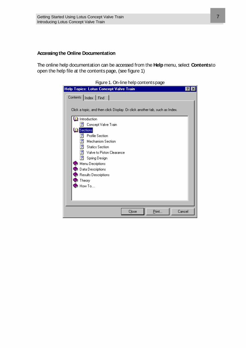
Accessing the Online Documentation The online help documentation can be accessed from the Help menu, select Contents to open the help file at the contents page, (see figure 1)
Figure 1. On-line help contents page
Getting Started Using Lotus Concept Valve Train Introducing Lotus Concept Valve Train
8
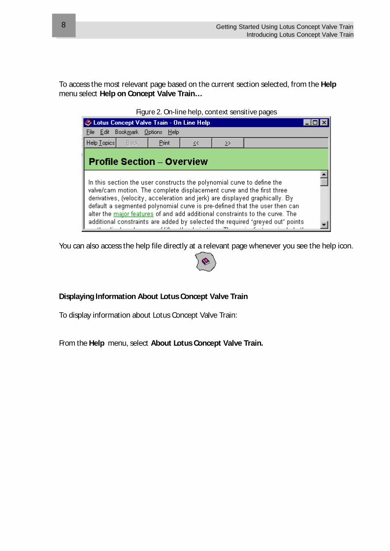
To access the most relevant page based on the current section selected, from the Help menu select Help on Concept Valve Train…
Figure 2. On-line help, context sensitive pages
You can also access the help file directly at a relevant page whenever you see the help icon.
Displaying Information About Lotus Concept Valve Train To display information about Lotus Concept Valve Train: From the Help menu, select About Lotus Concept Valve Train.
Overview This tutorial takes you through opening the application, introduces you to the menu structure, load an existing example model file and review the results. This tutorial includes the following sections:
n Starting Lotus Concept Valve Train, 10
n Familiarising Yourself with Lotus Concept Valve Train, 11
n Opening a Saved File, 12
n Direct Editing of Model Data, 12
n Viewing the Results Panel, 13
n Listing the Profile Incremental Results, 13
n The Use of Report Warnings, 14
n Closing the Application, 14
2 Tutorial 1. Getting Started
Getting Started Using Lotus Concept Valve Train Tutorial 1 ‘Getting Started’
10
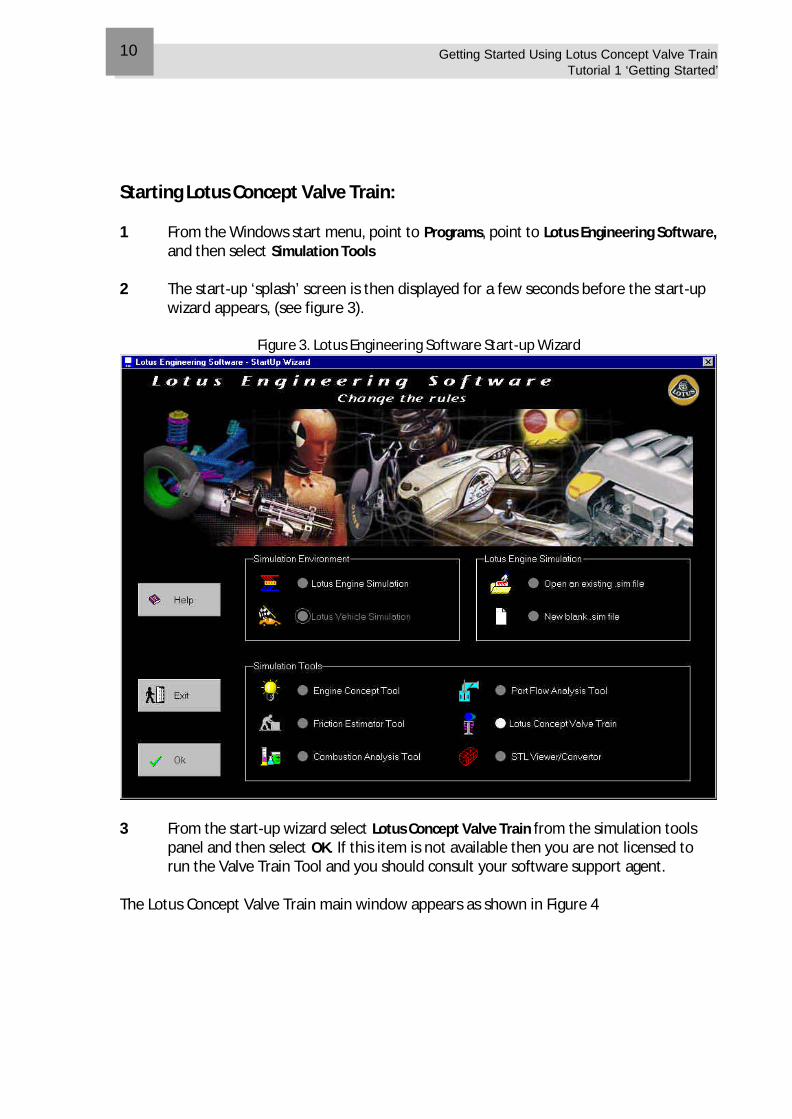
Starting Lotus Concept Valve Train: 1 From the Windows start menu, point to Programs, point to Lotus Engineering Software,
and then select Simulation Tools 2 The start-up ‘splash’ screen is then displayed for a few seconds before the start-up
wizard appears, (see figure 3).
Figure 3. Lotus Engineering Software Start-up Wizard
3 From the start-up wizard select Lotus Concept Valve Train from the simulation tools
panel and then select OK. If this item is not available then you are not licensed to run the Valve Train Tool and you should consult your software support agent.
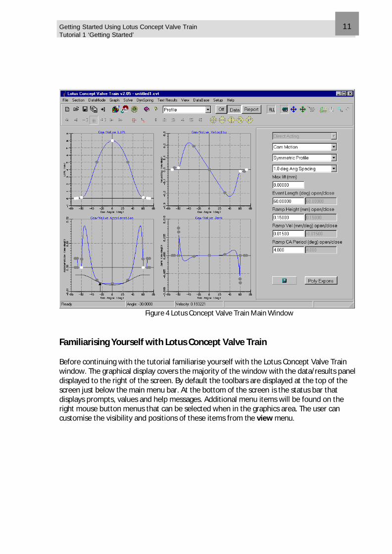
The Lotus Concept Valve Train main window appears as shown in Figure 4
Getting Started Using Lotus Concept Valve Train Tutorial 1 ‘Getting Started’
11
Figure 4 Lotus Concept Valve Train Main Window Familiarising Yourself with Lotus Concept Valve Train Before continuing with the tutorial familiarise yourself with the Lotus Concept Valve Train window. The graphical display covers the majority of the window with the data/results panel displayed to the right of the screen. By default the toolbars are displayed at the top of the screen just below the main menu bar. At the bottom of the screen is the status bar that displays prompts, values and help messages. Additional menu items will be found on the right mouse button menus that can be selected when in the graphics area. The user can customise the visibility and positions of these items from the view menu.
Getting Started Using Lotus Concept Valve Train Tutorial 1 ‘Getting Started’
12
Opening a Saved File Form the main menu File select Open, browse for the supplied example file Tutorial1.cvt, this should be located in the installation ‘examples’ sub-folder. Select ‘Ok’ to confirm the file open warning of data loss, (it should be noted that by default on opening the application is filled with default data for a direct acting system). When a file is loaded the calculations are automatically updated to refresh the displayed graphs and results. The standard ‘windows’ file browser dialog box is used to load the data file. The model data is arranged under six separate headings, ‘Profile’, ‘Mechanism’, ‘Statics’, ‘Valve/Piston clr’, ‘Spring Design’ and ‘Overlap’. Go through each of these main options using the selection box located in the toolbar to review the data associated with each section.
A number of the sections have additional data values accessed through the supplementary buttons normally labelled as ‘advanced’. Via these buttons, data values that are only seldom used can be edited.
Direct Editing of Model Data
We will now edit some of the default data to illustrate the process of data modifying and re-solving.
Pick the ‘Mechanism’ menu item and fit the graphical display to the available window, from the Graph menu, select Autoscale. The short cut key combination of Ctrl+A will also autoscale the display.
In the Valve Angle (deg) box enter 5.0.
In the Base Circle Radius box change the value to 18.0.
Getting Started Using Lotus Concept Valve Train Tutorial 1 ‘Getting Started’
13
Update the profile using the calculate button,
The solution can also be updated by using the Solve menu, select Update. The display will change to reflect the revised data.
Change the displayed section to ‘Statics’. In the System Effective Mass box enter 0.15 and update the profile.
Change the displayed section to ‘Valve/Piston Clr’. In the valve angle box enter 5.0. In the Perp Distance to Piston enter 2.2 and update the profile.
Now save the update data file. From the File menu, select Save_as and enter Tutorial1b in the filename box. Select Save.
Change the displayed section to ‘Profile’.
Viewing the Results Panel Change the side panel display to results, from the View menu, point to side panel, and then select Report.
The side panel ‘report’ displays a summary list of the current profiles main features. The use of a ‘red’ highlight is to indicate ‘at a glance’ items that do not meet the current analysis targets. All items should currently appear in grids having standard white backgrounds, (note depending on screen size you may need to scroll down to see all of the items in this list). See figure 5
Listing the Profile Incremental Results From the Text Results menu, select Display Valve Values. This will open a spread sheet displaying the incremental values for lift, velocity, acceleration and jerk for the valve end of the system. The displayed data can be copied into other applications using ‘cut and paste’, or saved to a text file using the local menu option File and select Save to File. For a direct acting system with a flat faced follower, the lift numbers can be used directly, to pass to the cam grinder.
Getting Started Using Lotus Concept Valve Train Tutorial 1 ‘Getting Started’
14
Figure 5. Side Panel changed to Report
The Use of Report Warnings The use of the report warnings is now reviewed. Change the side panel display to data, by using the View menu, point to side panel, and then select Data. Change the displayed section to ‘Mechanism’. In the Base Circle Radius box enter 16.0. Update the calculation. Change the side panel view back to Report. The grid background colour for maximum stress value will be shown in red.
The limits used for the report warnings can be set by the user to reflect your own specific requirements. From the Solve / Limit Settings menu select Edit cam limit settings… for the cam limits, select Edit valve limit settings… for the valve limits and select Edit statics limit settings or Edit statics(2) limit settings for the static analysis limits.
Closing the Application Now close the Lotus Concept Valve Train main window, from the File menu select Exit.
Overview This tutorial takes you through opening a new model, selecting the required model template, the options of defining either cam or valve motion and the alternative profile definition methods. This tutorial includes the following sections:
n Selecting a New Template Type, 16
n Changing the Motion Type, 17
n Viewing the Profile Segments, 17
n Closing the Application, 18
3 Tutorial 2. Reviewing Model Template Types
Getting Started Using Lotus Concept Valve Train Tutorial 2 ‘Reviewing Model Template Types’
16
Selecting a New Template Type Open the application as per tutorial 1 to get to the main Lotus Concept Valve Train Window, (Figure 4).
From the File menu, select New (all). Select ‘Ok’ to confirm the file new warning of data loss. This will display the new file dialog box, (see figure 6).
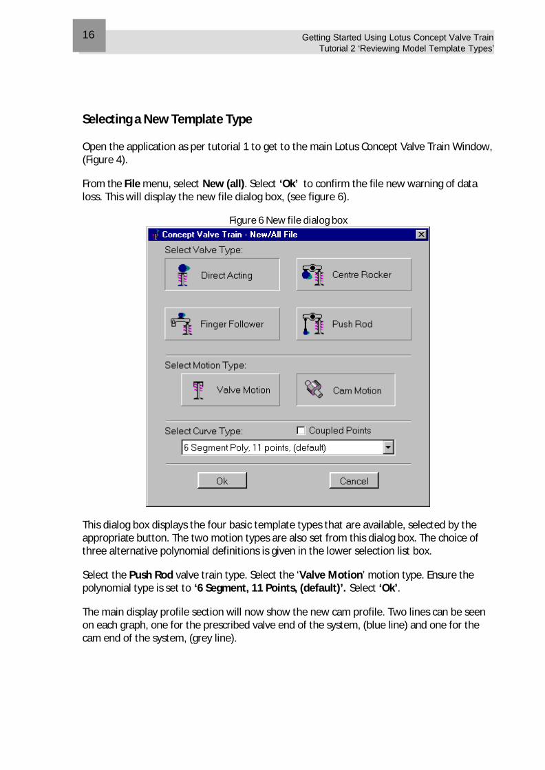
Figure 6 New file dialog box
This dialog box displays the four basic template types that are available, selected by the appropriate button. The two motion types are also set from this dialog box. The choice of three alternative polynomial definitions is given in the lower selection list box.
Select the Push Rod valve train type. Select the ‘Valve Motion’ motion type. Ensure the polynomial type is set to ‘6 Segment, 11 Points, (default)’. Select ‘Ok’.
The main display profile section will now show the new cam profile. Two lines can be seen on each graph, one for the prescribed valve end of the system, (blue line) and one for the cam end of the system, (grey line).
Getting Started Using Lotus Concept Valve Train Tutorial 2 ‘Reviewing Model Template Types’
17
Changing the Motion Type Repeat the steps above except this time select ‘Cam Motion’ as the motion type. Note that the main display now has the cam line draw in blue and the valve line draw in grey.
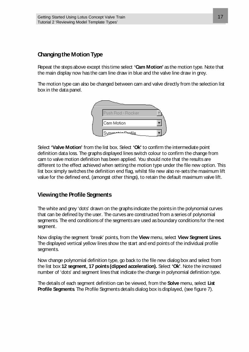
The motion type can also be changed between cam and valve directly from the selection list box in the data panel.
Select ‘Valve Motion’ from the list box. Select ‘Ok’ to confirm the intermediate point definition data loss. The graphs displayed lines switch colour to confirm the change from cam to valve motion definition has been applied. You should note that the results are different to the effect achieved when setting the motion type under the file new option. This list box simply switches the definition end flag, whilst file new also re-sets the maximum lift value for the defined end, (amongst other things), to retain the default maximum valve lift.
Viewing the Profile Segments The white and grey ‘dots’ drawn on the graphs indicate the points in the polynomial curves that can be defined by the user. The curves are constructed from a series of polynomial segments. The end conditions of the segments are used as boundary conditions for the next segment.
Now display the segment ‘break’ points, from the View menu, select View Segment Lines. The displayed vertical yellow lines show the start and end points of the individual profile segments.
Now change polynomial definition type, go back to the file new dialog box and select from the list box 12 segment, 17 points (clipped acceleration). Select ‘Ok’. Note the increased number of ‘dots’ and segment lines that indicate the change in polynomial definition type.
The details of each segment definition can be viewed, from the Solve menu, select List Profile Segments. The Profile Segments details dialog box is displayed, (see figure 7).
Getting Started Using Lotus Concept Valve Train Tutorial 2 ‘Reviewing Model Template Types’
18
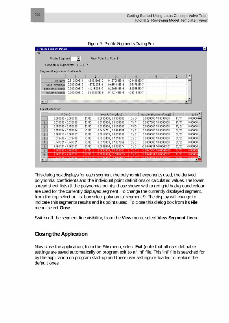
Figure 7. Profile Segments Dialog Box
This dialog box displays for each segment the polynomial exponents used, the derived polynomial coefficients and the individual point definitions or calculated values. The lower spread sheet lists all the polynomial points, those shown with a red grid background colour are used for the currently displayed segment. To change the currently displayed segment, from the top selection list box select polynomial segment 9. The display will change to indicate this segments results and its points used. To close this dialog box from its File menu, select Close.
Switch off the segment line visibility, from the View menu, select View Segment Lines.
Closing the Application Now close the application, from the File menu, select Exit (note that all user definable settings are saved automatically on program exit to a ‘.ini’ file. This ‘ini’ file is searched for by the application on program start-up and these user settings re-loaded to replace the default ones.
Overview This tutorial takes you through the steps of manipulating the data points used to define the profile polynomial for a direct acting system. The concepts of ‘edit’, ‘joggle’, ‘fix’ and ‘un-fix’ will be covered. The user will then manipulate the default profile to achieve target design values. This tutorial includes the following sections:
n Direct Editing of Profile Points, 20
n The Concepts of ‘fix’ and ‘un-fix’, 21
n Modifying a Profile Using Joggle, 21
4 Tutorial 3. Modifying the Cam Profile
Getting Started Using Lotus Concept Valve Train Tutorial 3 ‘Modifying the Cam Profile’
20
Direct Editing of Profile Points Open the Lotus Concept Valve Train program and load the previously saved file Tutorial1b.cvt
Ensure that the profile modify mode is set to edit, by selecting the edit button from the toolbar as indicated below.
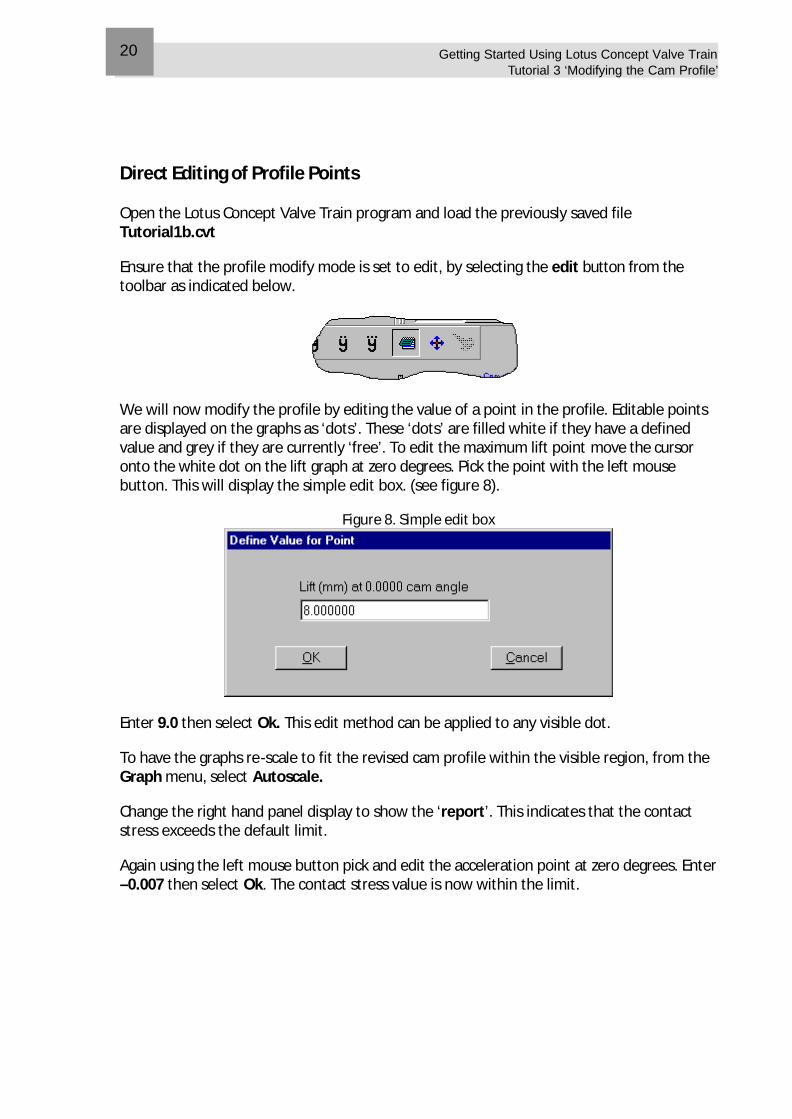
We will now modify the profile by editing the value of a point in the profile. Editable points are displayed on the graphs as ‘dots’. These ‘dots’ are filled white if they have a defined value and grey if they are currently ‘free’. To edit the maximum lift point move the cursor onto the white dot on the lift graph at zero degrees. Pick the point with the left mouse button. This will display the simple edit box. (see figure 8).
Figure 8. Simple edit box
Enter 9.0 then select Ok. This edit method can be applied to any visible dot.
To have the graphs re-scale to fit the revised cam profile within the visible region, from the Graph menu, select Autoscale.
Change the right hand panel display to show the ‘report’. This indicates that the contact stress exceeds the default limit.
Again using the left mouse button pick and edit the acceleration point at zero degrees. Enter –0.007 then select Ok. The contact stress value is now within the limit.
Getting Started Using Lotus Concept Valve Train Tutorial 3 ‘Modifying the Cam Profile’
21
The Concepts of ‘fix’ and ‘un-fix’ Points that have been edited (or fixed) by the user that are normally free can be unfixed by selecting the point with the right mouse button and pointing to UnFix Point. Unfix the previously defined acceleration value at zero degrees. This will return you to the profile with the high contact stress seen previously. (note all edit and unfix type actions automatically perform a solve update event)
Modifying a Profile Using Joggle
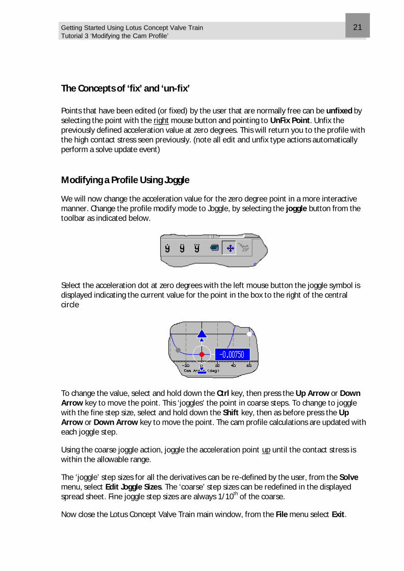
We will now change the acceleration value for the zero degree point in a more interactive manner. Change the profile modify mode to Joggle, by selecting the joggle button from the toolbar as indicated below.
Select the acceleration dot at zero degrees with the left mouse button the joggle symbol is displayed indicating the current value for the point in the box to the right of the central circle
To change the value, select and hold down the Ctrl key, then press the Up Arrow or Down Arrow key to move the point. This ‘joggles’ the point in coarse steps. To change to joggle with the fine step size, select and hold down the Shift key, then as before press the Up Arrow or Down Arrow key to move the point. The cam profile calculations are updated with each joggle step.
Using the coarse joggle action, joggle the acceleration point up until the contact stress is within the allowable range.
The ‘joggle’ step sizes for all the derivatives can be re-defined by the user, from the Solve menu, select Edit Joggle Sizes. The ‘coarse’ step sizes can be redefined in the displayed spread sheet. Fine joggle step sizes are always 1/10th of the coarse.
Now close the Lotus Concept Valve Train main window, from the File menu select Exit.

Getting Started Using Lotus Concept Valve Train Tutorial 3 ‘Modifying the Cam Profile’
22
Overview This tutorial takes you through the steps of manipulating the data points used to define the mechanism geometry for a default push rod system. The concepts of ‘edit’ and ‘joggle’ will be covered. The user will then manipulate the default geometry to achieve target design values. This tutorial includes the following sections:
n Displaying the Mechanism Graphics, 24
n Direct Editing of the Mechanism, 24
n Editing of the Mechanism Through the Display, 25
n Application of Joggle to the Mechanism Geometry, 26
n Design Exercise, 26
5 Tutorial 4. Modifying the Mechanism
Getting Started Using Lotus Concept Valve Train Tutorial 4 ‘Modifying the Mechanism’
24
Displaying the Mechanism Graphics Open the Lotus Concept Valve Train program. From the File menu select new (all). Select ‘Ok’ to confirm the file new warning of data loss. This will display the new file dialog box, (see figure 6).
Set the valve train type to Push Rod and the motion type to Cam Motion. Ensure the polynomial type is set to the default 6 segment, 11 Points.
Change the displayed section to Mechanism and set the modify mode to edit by selecting the Edit icon from the toolbar as indicated below.
Autoscale the graphical display of the mechanism by selecting the keys Ctrl+A. Direct Editing of the Mechanism We will now review the number of ways that the geometry can be manipulated. Firstly by direct editing in the data panel….
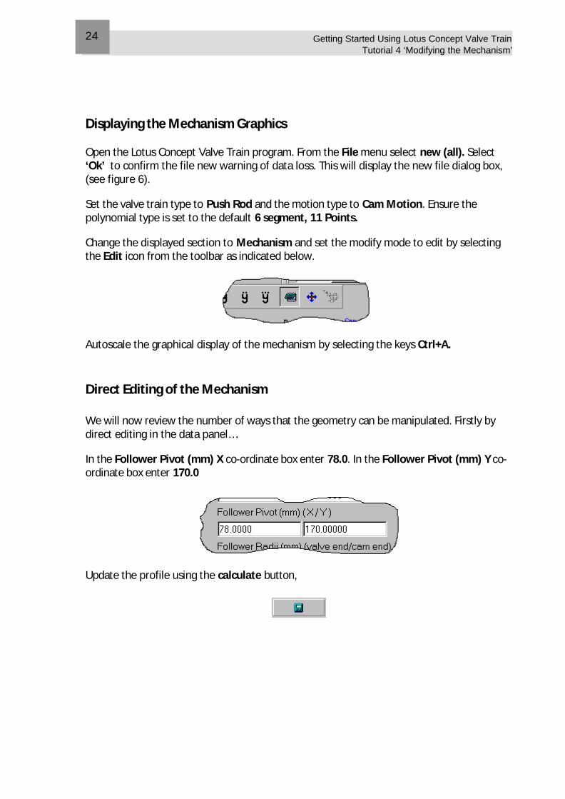
In the Follower Pivot (mm) X co-ordinate box enter 78.0. In the Follower Pivot (mm) Y co-ordinate box enter 170.0
Update the profile using the calculate button,
Getting Started Using Lotus Concept Valve Train Tutorial 4 ‘Modifying the Mechanism’
25
Editing of the Mechanism Through the Display Now we will edit the geometry using the graphical display….
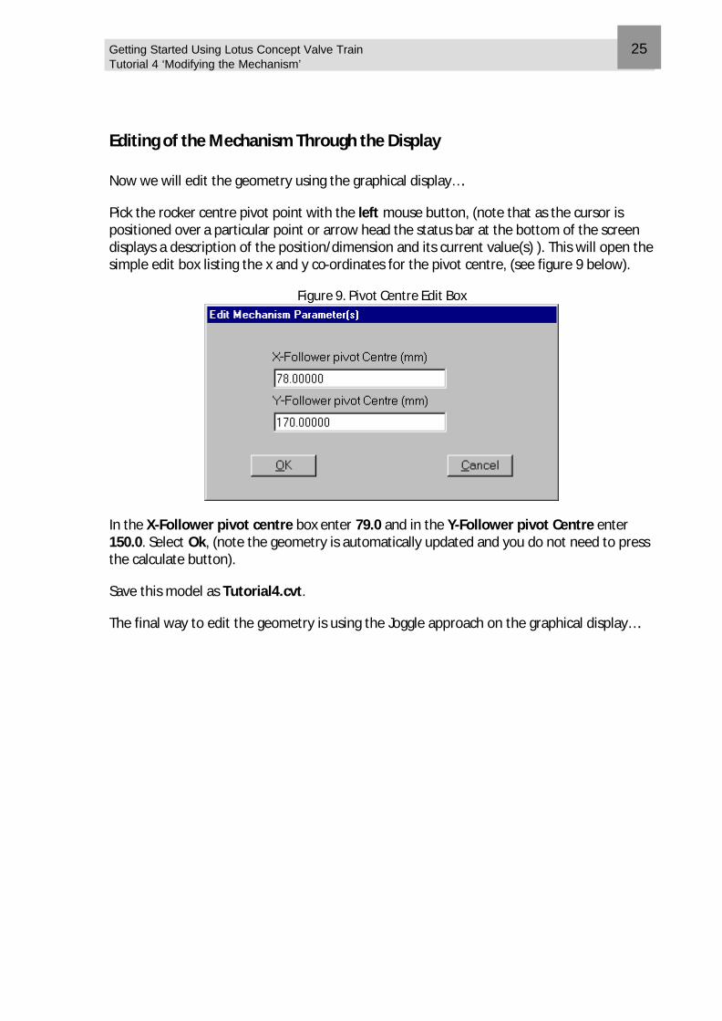
Pick the rocker centre pivot point with the left mouse button, (note that as the cursor is positioned over a particular point or arrow head the status bar at the bottom of the screen displays a description of the position/dimension and its current value(s) ). This will open the simple edit box listing the x and y co-ordinates for the pivot centre, (see figure 9 below).
Figure 9. Pivot Centre Edit Box
In the X-Follower pivot centre box enter 79.0 and in the Y-Follower pivot Centre enter 150.0. Select Ok, (note the geometry is automatically updated and you do not need to press the calculate button).
Save this model as Tutorial4.cvt.
The final way to edit the geometry is using the Joggle approach on the graphical display….
Getting Started Using Lotus Concept Valve Train Tutorial 4 ‘Modifying the Mechanism’
26
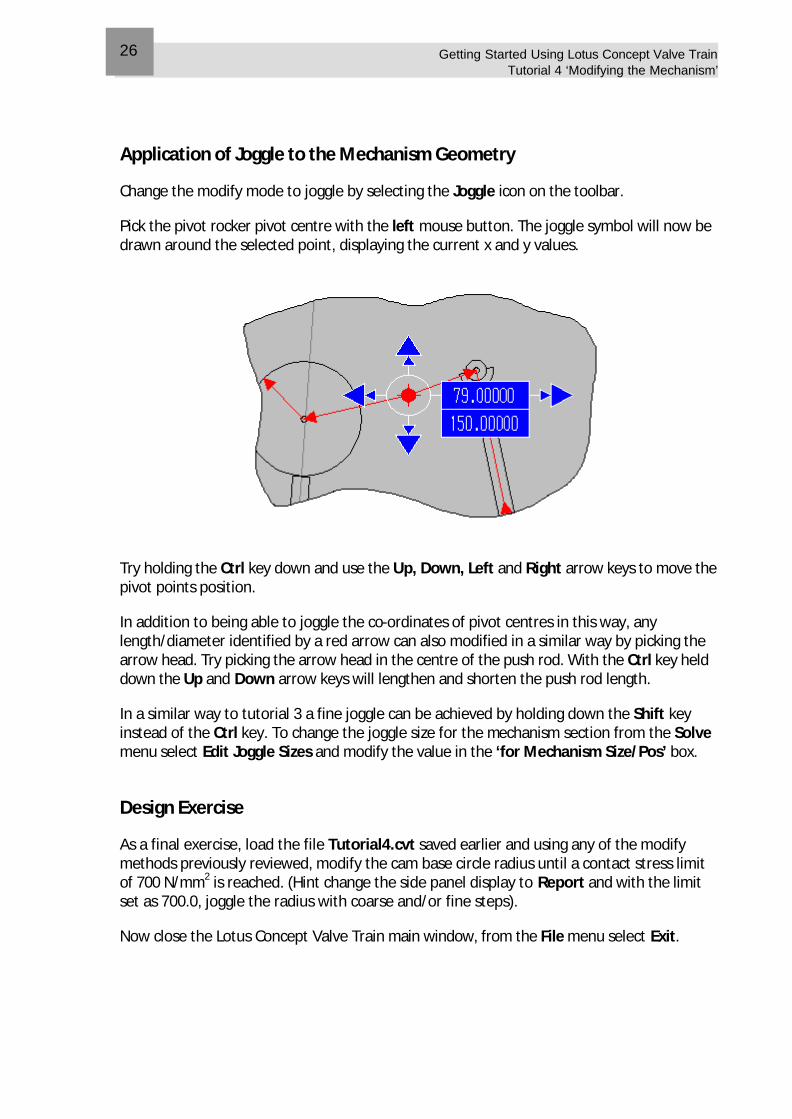
Application of Joggle to the Mechanism Geometry
Change the modify mode to joggle by selecting the Joggle icon on the toolbar.
Pick the pivot rocker pivot centre with the left mouse button. The joggle symbol will now be drawn around the selected point, displaying the current x and y values.
Try holding the Ctrl key down and use the Up, Down, Left and Right arrow keys to move the pivot points position.
In addition to being able to joggle the co-ordinates of pivot centres in this way, any length/diameter identified by a red arrow can also modified in a similar way by picking the arrow head. Try picking the arrow head in the centre of the push rod. With the Ctrl key held down the Up and Down arrow keys will lengthen and shorten the push rod length.
In a similar way to tutorial 3 a fine joggle can be achieved by holding down the Shift key instead of the Ctrl key. To change the joggle size for the mechanism section from the Solve menu select Edit Joggle Sizes and modify the value in the ‘for Mechanism Size/Pos’ box.
Design Exercise
As a final exercise, load the file Tutorial4.cvt saved earlier and using any of the modify methods previously reviewed, modify the cam base circle radius until a contact stress limit of 700 N/mm2 is reached. (Hint change the side panel display to Report and with the limit set as 700.0, joggle the radius with coarse and/or fine steps).
Now close the Lotus Concept Valve Train main window, from the File menu select Exit.
Overview This tutorial aims to help you understand how to turn typical ‘real world’ geometry into an equivalent Lotus Concept Valve Train analytical model. Simple steps are used to take the information from a dimensioned scheme and modify the appropriate default template data. This tutorial includes the following sections:
n Reviewing supplied geometry, 28
n Opening the application and loading required template, 28
n Modifying the template geometry, 29
n Assessing the lift limitations, 32
Tutorial 5. A Real Example 6
Getting Started Using Lotus Concept Valve Train Tutorial 5 ‘A Real Example’
28
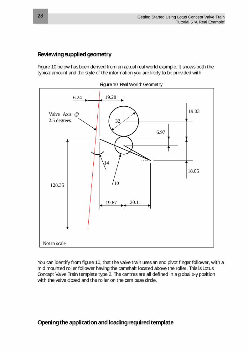
Reviewing supplied geometry Figure 10 below has been derived from an actual real world example. It shows both the typical amount and the style of the information you are likely to be provided with.
Figure 10 ‘Real World’ Geometry
You can identify from figure 10, that the valve train uses an end pivot finger follower, with a mid mounted roller follower having the camshaft located above the roller. This is Lotus Concept Valve Train template type 2. The centres are all defined in a global x-y position with the valve closed and the roller on the cam base circle. Opening the application and loading required template
19.67 20.11
6.97
18.06
128.35
19.28 6.24
19.03
32
10
14
Valve Axis @ 2.5 degrees
Not to scale
Getting Started Using Lotus Concept Valve Train Tutorial 5 ‘A Real Example’
29
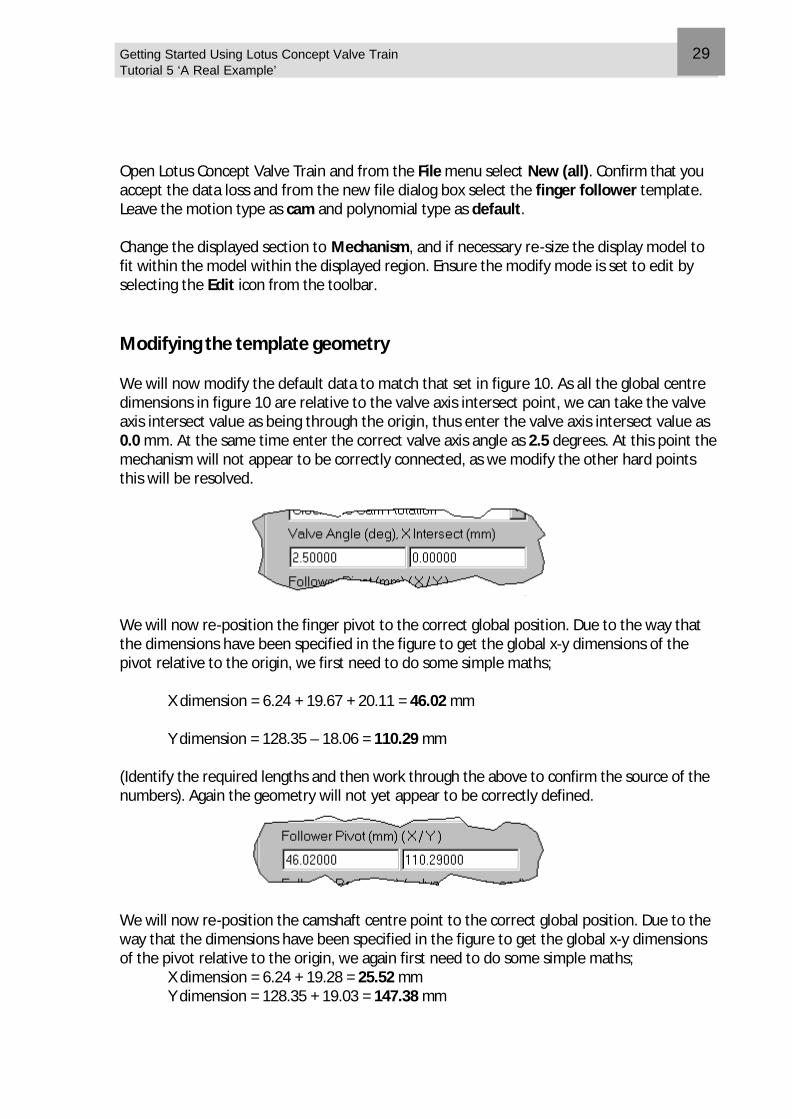
Open Lotus Concept Valve Train and from the File menu select New (all). Confirm that you accept the data loss and from the new file dialog box select the finger follower template. Leave the motion type as cam and polynomial type as default. Change the displayed section to Mechanism, and if necessary re-size the display model to fit within the model within the displayed region. Ensure the modify mode is set to edit by selecting the Edit icon from the toolbar. Modifying the template geometry We will now modify the default data to match that set in figure 10. As all the global centre dimensions in figure 10 are relative to the valve axis intersect point, we can take the valve axis intersect value as being through the origin, thus enter the valve axis intersect value as 0.0 mm. At the same time enter the correct valve axis angle as 2.5 degrees. At this point the mechanism will not appear to be correctly connected, as we modify the other hard points this will be resolved.
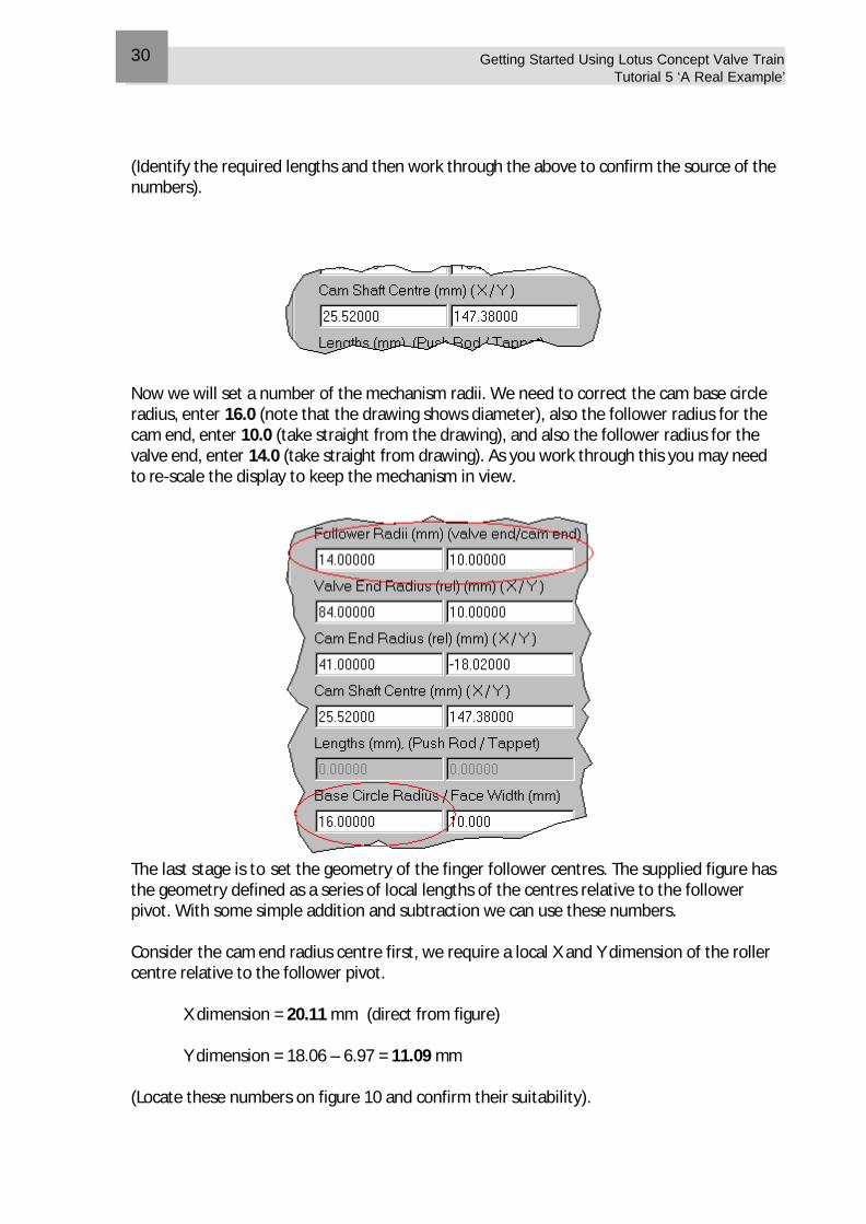
We will now re-position the finger pivot to the correct global position. Due to the way that the dimensions have been specified in the figure to get the global x-y dimensions of the pivot relative to the origin, we first need to do some simple maths; X dimension = 6.24 + 19.67 + 20.11 = 46.02 mm Y dimension = 128.35 – 18.06 = 110.29 mm (Identify the required lengths and then work through the above to confirm the source of the numbers). Again the geometry will not yet appear to be correctly defined.
We will now re-position the camshaft centre point to the correct global position. Due to the way that the dimensions have been specified in the figure to get the global x-y dimensions of the pivot relative to the origin, we again first need to do some simple maths; X dimension = 6.24 + 19.28 = 25.52 mm Y dimension = 128.35 + 19.03 = 147.38 mm
Getting Started Using Lotus Concept Valve Train Tutorial 5 ‘A Real Example’
30
(Identify the required lengths and then work through the above to confirm the source of the numbers).
Now we will set a number of the mechanism radii. We need to correct the cam base circle radius, enter 16.0 (note that the drawing shows diameter), also the follower radius for the cam end, enter 10.0 (take straight from the drawing), and also the follower radius for the valve end, enter 14.0 (take straight from drawing). As you work through this you may need to re-scale the display to keep the mechanism in view.
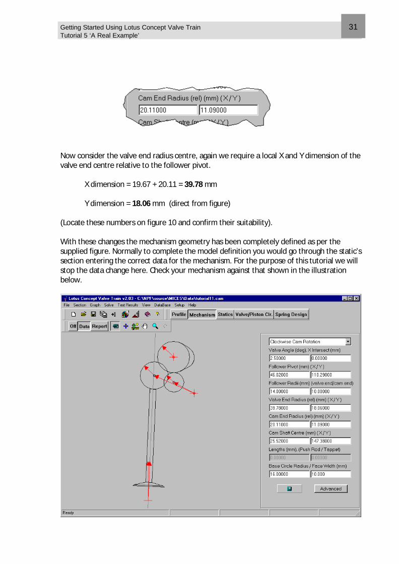
The last stage is to set the geometry of the finger follower centres. The supplied figure has the geometry defined as a series of local lengths of the centres relative to the follower pivot. With some simple addition and subtraction we can use these numbers. Consider the cam end radius centre first, we require a local X and Y dimension of the roller centre relative to the follower pivot. X dimension = 20.11 mm (direct from figure) Y dimension = 18.06 – 6.97 = 11.09 mm (Locate these numbers on figure 10 and confirm their suitability).
Getting Started Using Lotus Concept Valve Train Tutorial 5 ‘A Real Example’
31
Now consider the valve end radius centre, again we require a local X and Y dimension of the valve end centre relative to the follower pivot. X dimension = 19.67 + 20.11 = 39.78 mm Y dimension = 18.06 mm (direct from figure) (Locate these numbers on figure 10 and confirm their suitability). With these changes the mechanism geometry has been completely defined as per the supplied figure. Normally to complete the model definition you would go through the static’s section entering the correct data for the mechanism. For the purpose of this tutorial we will stop the data change here. Check your mechanism against that shown in the illustration below.
Getting Started Using Lotus Concept Valve Train Tutorial 5 ‘A Real Example’
32
Assessing the lift limitations This example typifies the profile concavity problems seen on valve train systems with small radius followers. Change the display to Report, note that the minimum –ve radius is –81.3 mm, (-ve implies concave). With the simple polynomial definition method the cam lift has to be reduced down to 4.0 mm before the camshaft becomes convex. Exercise; Try repeating this tutorial but use the clipped acceleration polynomial definition instead of the default. This polynomial type is specifically for coping with concave cams. See what maximum lift you can achieve this time.
Overview This tutorial looks at the data requirements of the static’s section. The influence of data variables on the ability to achieve design targets is examined. The user will modify spring data to achieve target design values. This tutorial includes the following sections:
n Static’s Data Variables, 34
n Spring Cover, 34
n Hertzian Contact Stress, 35
n Design Exercise, 35
n Design Exercise Results, 36
7 Tutorial 6. Reviewing Static’s Data
Getting Started Using Lotus Concept Valve Train Tutorial 6 ‘Reviewing Static’s Data’
34
Static’s Data Variables Open the Lotus Concept Valve Train program. From the File menu select new (all). Select ‘Ok’ to confirm the file new warning of data loss. This will display the new file dialog box, (see figure 6). Select the Finger Follower type, select motion type as Cam Motion. Ensure the polynomial type is set to 6 Points, 11 Segments (default). Select the Static’s button, and ensure the side panel display is set to Data. To fit the graphs to the available space, from the Graph menu select Autoscale. Choose to display a single graph only. Use the right mouse menu and select Graph View / Position 2 from the popup menu. This will change the graphs displayed to show only the one graph. To revert back to all six graphs select Graph View / All. Spring Cover The Spring cover graph shows the spring and inertia load lines for the cam and valve ends of the system. In the Design Speed (rpm) box enter 4500.0. Update the static analysis using the calculate button. (Note the change to the inertia load curve) In the Spring Preload (N) box enter 110.0 for the outer spring. (Note that there are two boxes, one for the outer spring and one for the inner spring, if the valve train has only one spring leave one as zero.). In the Spring Rate (N/mm) box enter 20.0 for the outer spring. (Note as for preload above there are two boxes, leave the inner as zero). Update the static analysis using the calculate button. (Note the change to the spring load curve).
Getting Started Using Lotus Concept Valve Train Tutorial 6 ‘Reviewing Static’s Data’
35
Hertzian Contact Stress Change the graph display to the contact stress plot, by selecting the relevant position/menu from the right mouse menu. This will change the graph displayed to show only the graph of contact stress between the cam and the follower. The two lines show the calculated stress for the ‘zero speed’ and the ‘design speed’ conditions. In the Cam Face Width (mm) box enter 12.0. Update the calculation. (Note that the stress values drop for both speed conditions). In the System Effective mass (kg) box enter 0.18. Update the calculation. (Note that only the stress values for the ‘design speed’ condition change. Increasing at the flank conditions due to the addition of spring and inertia, decreasing over the nose, due to the subtraction of spring and inertia). Design Exercise To put what we have learned to the test, we will now identify a design specification that meets two simple targets. Starting from the modified data values that we have, you can only change the spring preload, spring rate and cam face width to achieve a float speed 6500 rpm and a maximum contact stress of 700 N/mm2. Hint 1: Change the graph display to ALL. Remember to switch between Data and Report to show latest results and to Update the calculation after data changes. Hint 2: In the Design speed box enter 6500.0. Hint 3: Start by achieving the target float speed then increase the cam face width to bring the contact stress down to the required value. Hint 4: Start from a spring preload value of 250.0 N and ramp up the spring rate to achieve the target float speed.
Getting Started Using Lotus Concept Valve Train Tutorial 6 ‘Reviewing Static’s Data’
36
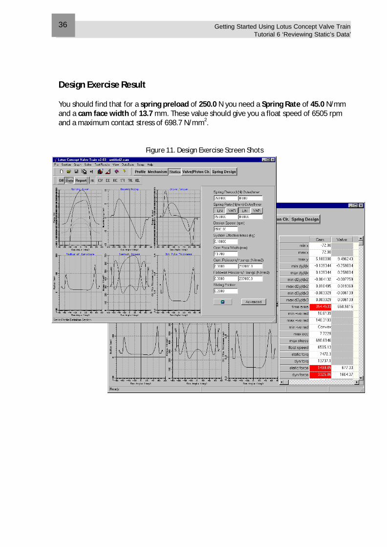
Design Exercise Result You should find that for a spring preload of 250.0 N you need a Spring Rate of 45.0 N/mm and a cam face width of 13.7 mm. These value should give you a float speed of 6505 rpm and a maximum contact stress of 698.7 N/mm2.
Figure 11. Design Exercise Screen Shots
Overview This tutorial covers the valve to piston clearance section. The user will identify the limiting valve timing for adequate valve clearance. This tutorial includes the following sections:
n Piston Clearance Valve Lift Data Variables, 38
n Piston Clearance, Engine Geometry Data Variables, 39
n Piston Clearance, Valve Geometry Data Variables, 39
n Design Exercise, 40
n Design Exercise Result, 41
8 Tutorial 7. A Look at Valve to Piston clearance
Getting Started Using Lotus Concept Valve Train Tutorial 7 ‘A Look at Valve to Piston Clearance’
38
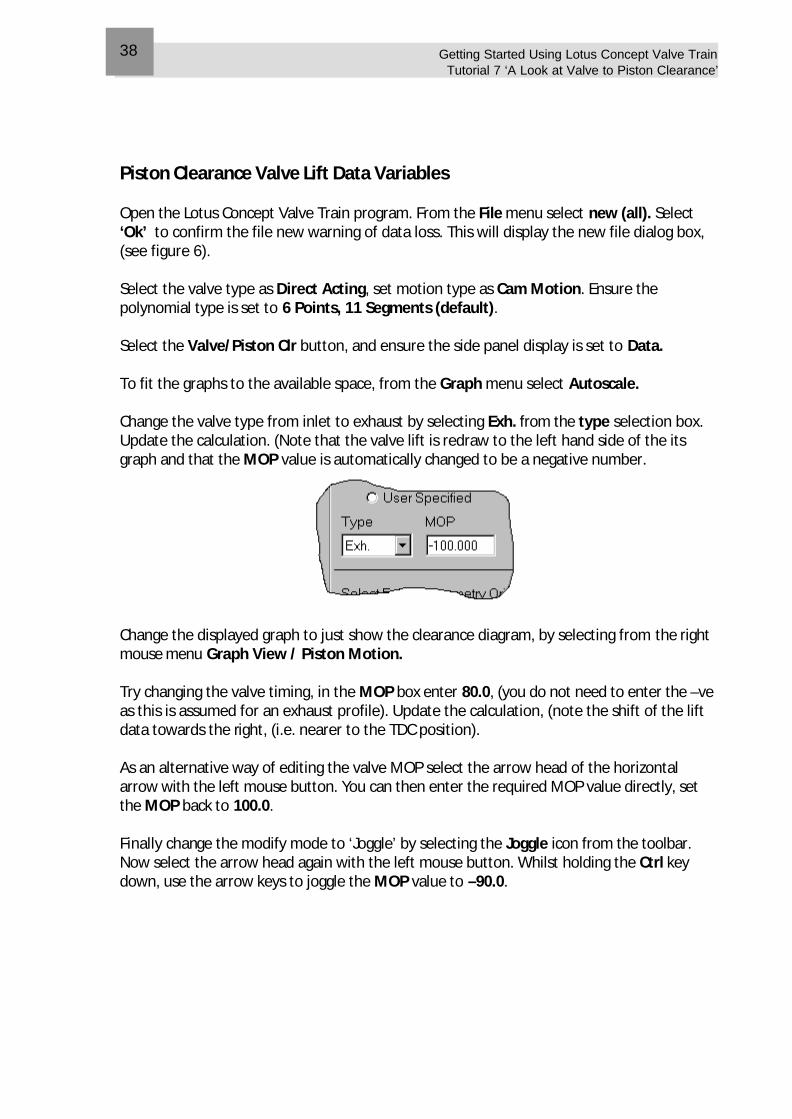
Piston Clearance Valve Lift Data Variables Open the Lotus Concept Valve Train program. From the File menu select new (all). Select ‘Ok’ to confirm the file new warning of data loss. This will display the new file dialog box, (see figure 6). Select the valve type as Direct Acting, set motion type as Cam Motion. Ensure the polynomial type is set to 6 Points, 11 Segments (default). Select the Valve/Piston Clr button, and ensure the side panel display is set to Data. To fit the graphs to the available space, from the Graph menu select Autoscale. Change the valve type from inlet to exhaust by selecting Exh. from the type selection box. Update the calculation. (Note that the valve lift is redraw to the left hand side of the its graph and that the MOP value is automatically changed to be a negative number.
Change the displayed graph to just show the clearance diagram, by selecting from the right mouse menu Graph View / Piston Motion. Try changing the valve timing, in the MOP box enter 80.0, (you do not need to enter the –ve as this is assumed for an exhaust profile). Update the calculation, (note the shift of the lift data towards the right, (i.e. nearer to the TDC position). As an alternative way of editing the valve MOP select the arrow head of the horizontal arrow with the left mouse button. You can then enter the required MOP value directly, set the MOP back to 100.0. Finally change the modify mode to ‘Joggle’ by selecting the Joggle icon from the toolbar. Now select the arrow head again with the left mouse button. Whilst holding the Ctrl key down, use the arrow keys to joggle the MOP value to –90.0.
Getting Started Using Lotus Concept Valve Train Tutorial 7 ‘A Look at Valve to Piston Clearance’
39
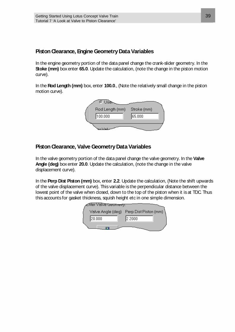
Piston Clearance, Engine Geometry Data Variables In the engine geometry portion of the data panel change the crank-slider geometry. In the Stoke (mm) box enter 65.0. Update the calculation, (note the change in the piston motion curve). In the Rod Length (mm) box, enter 100.0., (Note the relatively small change in the piston motion curve).
Piston Clearance, Valve Geometry Data Variables In the valve geometry portion of the data panel change the valve geometry. In the Valve Angle (deg) box enter 20.0. Update the calculation, (note the change in the valve displacement curve). In the Perp Dist Piston (mm) box, enter 2.2. Update the calculation, (Note the shift upwards of the valve displacement curve). This variable is the perpendicular distance between the lowest point of the valve when closed, down to the top of the piston when it is at TDC. Thus this accounts for gasket thickness, squish height etc in one simple dimension.

Getting Started Using Lotus Concept Valve Train Tutorial 7 ‘A Look at Valve to Piston Clearance’
40
Design Exercise From the currently defined data identify the limiting valve timing (MOP’s) for both an inlet and exhaust camshaft, if the target minimum valve clearance is based on 10% of maximum lift. Hint 1: Change the side panel display to Report, (you may need to scroll down the report listing to display min valve clear). Hint 2: Change the modify mode to Joggle and use joggle on the horizontal MOP arrow head. Hint 3: For the peak valve lift of 8.0 mm, the minimum clearance required is 0.8mm (i.e. 10% of maximum lift).
Getting Started Using Lotus Concept Valve Train Tutorial 7 ‘A Look at Valve to Piston Clearance’
41
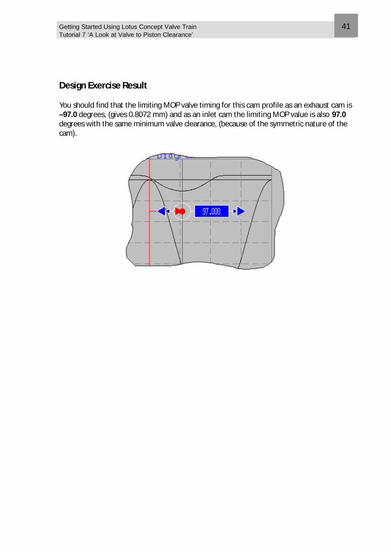
Design Exercise Result You should find that the limiting MOP valve timing for this cam profile as an exhaust cam is –97.0 degrees, (gives 0.8072 mm) and as an inlet cam the limiting MOP value is also 97.0 degrees with the same minimum valve clearance, (because of the symmetric nature of the cam).

Getting Started Using Lotus Concept Valve Train Tutorial 7 ‘A Look at Valve to Piston Clearance’
42
Overview This tutorial reviews the data associated with the spring section. You will then produce a progressive rate valve spring design that is applied to an existing valve train model to look at the influence of the spring design on the valve train static’s. This tutorial includes the following sections:
n Screen Layout, 44
n Graphical Options, 44
n Spring Design Data, 45
n Spring Design Options, 46
n Design Exercise, 46
n Application to Valve Train Static’s, 47
9 Tutorial 8. Spring Design
Getting Started Using Lotus Concept Valve Train Tutorial 8 ‘Spring Design’
44
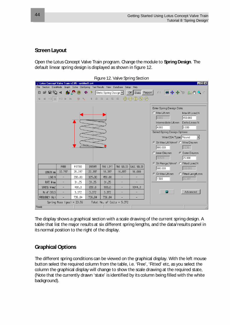
Screen Layout Open the Lotus Concept Valve Train program. Change the module to Spring Design. The default linear spring design is displayed as shown in figure 12.
Figure 12. Valve Spring Section
The display shows a graphical section with a scale drawing of the current spring design. A table that list the major results at six different spring lengths, and the data/results panel in its normal position to the right of the display. Graphical Options The different spring conditions can be viewed on the graphical display. With the left mouse button select the required column from the table, i.e. ‘Free’, ‘Fitted’ etc, as you select the column the graphical display will change to show the scale drawing at the required state, (Note that the currently drawn ‘state’ is identified by its column being filled with the white background).
Getting Started Using Lotus Concept Valve Train Tutorial 8 ‘Spring Design’
45
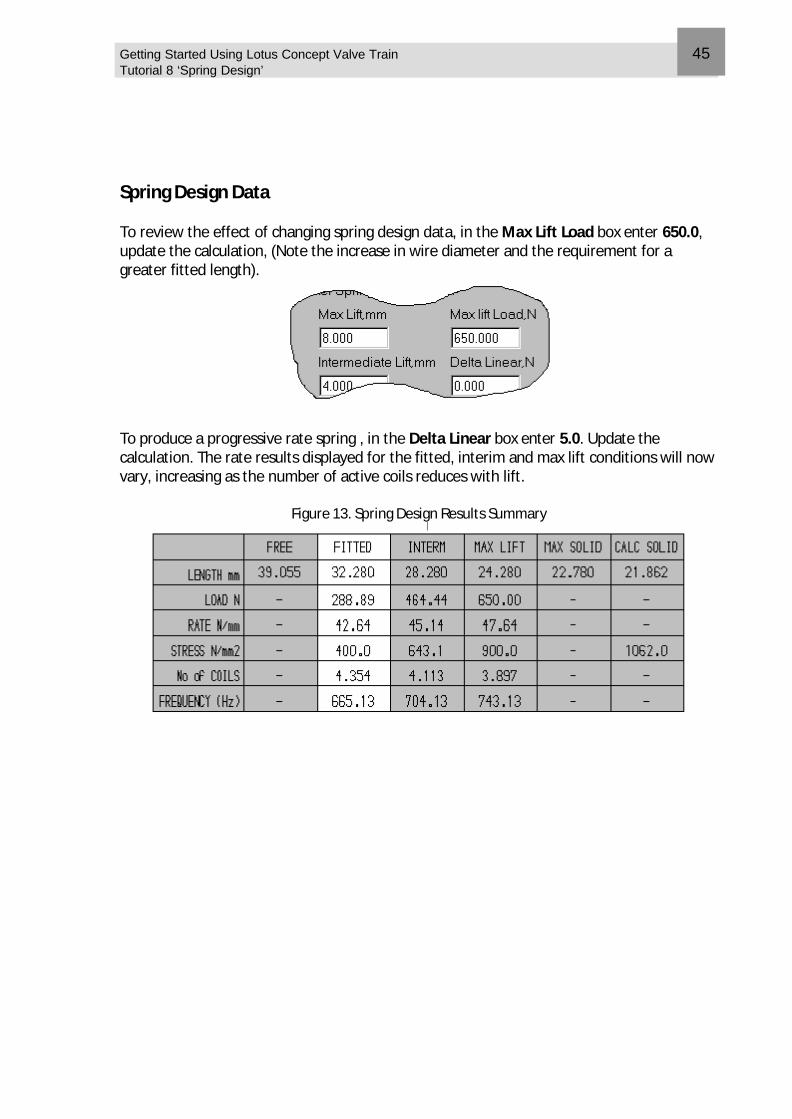
Spring Design Data To review the effect of changing spring design data, in the Max Lift Load box enter 650.0, update the calculation, (Note the increase in wire diameter and the requirement for a greater fitted length).
To produce a progressive rate spring , in the Delta Linear box enter 5.0. Update the calculation. The rate results displayed for the fitted, interim and max lift conditions will now vary, increasing as the number of active coils reduces with lift.
Figure 13. Spring Design Results Summary
Getting Started Using Lotus Concept Valve Train Tutorial 8 ‘Spring Design’
46
Spring Design Options A number of choices are provided in the definition of the spring design. These are presented as toggle selections in the Spring Design Options section of the data panel. They require four selections to be made: n Define wire diameter by stress at maximum lift, or define the wire diameter directly. n Set the overall spring diameter by either the outer diameter or the inner diameter of
the coils. n Set the spring load condition either by stress range between the fitted and the fully
open points, or set the fitted load directly. n Set the fitted length either by the clearance to the solid condition at maximum lift or
set the fitted length directly. As an example of how this is implemented. Check the toggle box next to the Fitted Length option. This will initially make no change to the display other than to grey out the edit box for ‘clr max lift’ and enable the edit box for ‘Fitted Length’. In the Fitted Length box, enter 35.0. Update the calculation, (Note the change in fitted length). Design Exercise We will now design a simple progressive rate spring and load the designed spring curve into the valve train static’s data section as an additional inner spring to the existing outer spring.
1 In the Max Lift Load box, enter 250.0. 2 In the Delta Linear box, enter 2.0. 3 Ensure the Str Max Lift toggle is checked and set to 900.0. 4 Ensure the Outer Dia toggle is checked and enter 16.0 in the Outer Dia box.
5 Ensure the Str Range toggle is checked and set to 500.0.
6 Ensure the Clr Max Lift toggle is checked and set to 1.5.
7 Update the calculation.
Getting Started Using Lotus Concept Valve Train Tutorial 8 ‘Spring Design’
47
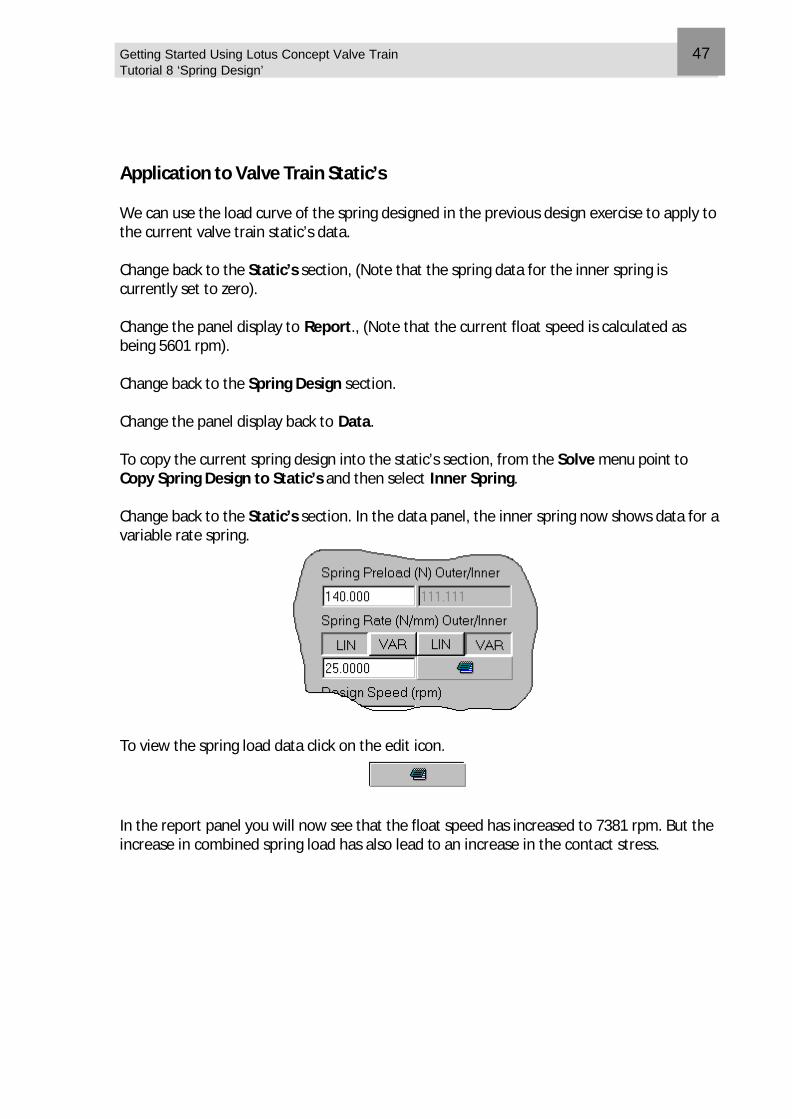
Application to Valve Train Static’s We can use the load curve of the spring designed in the previous design exercise to apply to the current valve train static’s data. Change back to the Static’s section, (Note that the spring data for the inner spring is currently set to zero). Change the panel display to Report., (Note that the current float speed is calculated as being 5601 rpm). Change back to the Spring Design section. Change the panel display back to Data. To copy the current spring design into the static’s section, from the Solve menu point to Copy Spring Design to Static’s and then select Inner Spring. Change back to the Static’s section. In the data panel, the inner spring now shows data for a variable rate spring.
To view the spring load data click on the edit icon.
In the report panel you will now see that the float speed has increased to 7381 rpm. But the increase in combined spring load has also lead to an increase in the contact stress.

Getting Started Using Lotus Concept Valve Train Tutorial 8 ‘Spring Design’
48
Overview You will export a previously created model out to an Adams Engine model file. The concepts of Templates, subsystems and component files will be covered as they pertain to Lotus Concept Valve Train. If available Adams Engine will be started from within Lotus Concept Valve Train and this saved model loaded into Adams Engine. This tutorial includes the following sections:
n Preparing for Export, 50
n Exporting the Cam Profile, 50
n Exporting the Sub-System Model, 52
n Exporting Directly from the Preview, 52
n Preparing to Run ADAMS/Engine, 53
n Running ADAMS/Engine, 54 Note: To be able to fully complete this tutorial you will need to be licensed on ADAMS/EngineTM Valve Train Module.
10 Tutorial 9. Export of Data
Getting Started Using Lotus Concept Valve Train Tutorial 9 ‘Export of Data’
50
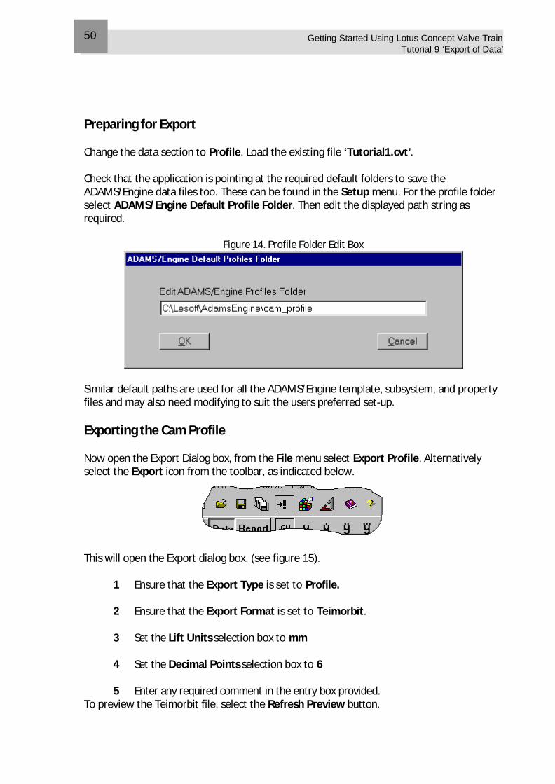
Preparing for Export Change the data section to Profile. Load the existing file ‘Tutorial1.cvt’. Check that the application is pointing at the required default folders to save the ADAMS/Engine data files too. These can be found in the Setup menu. For the profile folder select ADAMS/Engine Default Profile Folder. Then edit the displayed path string as required.
Figure 14. Profile Folder Edit Box
Similar default paths are used for all the ADAMS/Engine template, subsystem, and property files and may also need modifying to suit the users preferred set-up. Exporting the Cam Profile Now open the Export Dialog box, from the File menu select Export Profile. Alternatively select the Export icon from the toolbar, as indicated below.
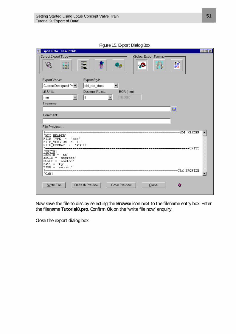
This will open the Export dialog box, (see figure 15).
1 Ensure that the Export Type is set to Profile. 2 Ensure that the Export Format is set to Teimorbit. 3 Set the Lift Units selection box to mm 4 Set the Decimal Points selection box to 6
5 Enter any required comment in the entry box provided.
To preview the Teimorbit file, select the Refresh Preview button.
Getting Started Using Lotus Concept Valve Train Tutorial 9 ‘Export of Data’
51
Figure 15. Export Dialog Box
Now save the file to disc by selecting the Browse icon next to the filename entry box. Enter the filename Tutorial8.pro. Confirm Ok on the ‘write file now’ enquiry. Close the export dialog box.
Getting Started Using Lotus Concept Valve Train Tutorial 9 ‘Export of Data’
52
Exporting the Sub-System Model Open the export dialog box, from the File menu select Export SubSystem. From the Tappet Type selection box, select Hydraulic Tappet. Ensure the Profile Filename box has the previously saved Tutorial8.pro name displayed. To preview the Sub-System Teimorbit file, select the Subsystem button above the file preview area, then pick the Refresh Preview button. Now save the file to disc by selecting the Browse icon next to the filename entry box. Enter the filename Tutorial8.sub. Confirm Ok on the ‘write file now’ enquiry. This will export not only the sub-system file, but also the six UDE property files that the sub-system file references. Exporting Directly from the Preview The previous export action wrote out all the individual property files in one go. The File preview display can be used to either export property files individually or also modify the previewed file and then save it. Select the Cam button above the file preview area. The preview display will change to list the cam UDE property file. Scroll down the display until you can see an entry for Width. Change the displayed value to 12.0. Clear the Subsystem Filename box. Then select the Save Preview button to store the modified file. Browse to find the existing cam file. Select Ok to confirm the overwrite of the existing file. Close the export dialog box..
Getting Started Using Lotus Concept Valve Train Tutorial 9 ‘Export of Data’
53
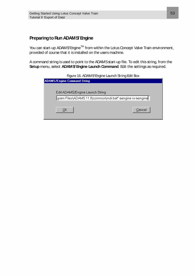
Preparing to Run ADAMS/Engine You can start-up ADAMS/EngineTM from within the Lotus Concept Valve Train environment, provided of course that it is installed on the users machine. A command string is used to point to the ADAMS start-up file. To edit this string, from the Setup menu, select ADAMS/Engine Launch Command. Edit the settings as required.
Figure 16. ADAMS/Engine Launch String Edit Box
Getting Started Using Lotus Concept Valve Train Tutorial 9 ‘Export of Data’
54
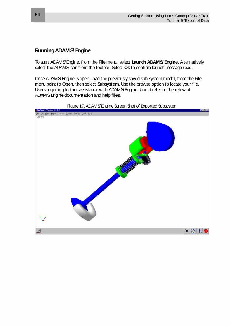
Running ADAMS/Engine To start ADAMS/Engine, from the File menu, select Launch ADAMS/Engine. Alternatively select the ADAMS icon from the toolbar. Select Ok to confirm launch message read. Once ADAMS/Engine is open, load the previously saved sub-system model, from the File menu point to Open, then select Subsystem. Use the browse option to locate your file. Users requiring further assistance with ADAMS/Engine should refer to the relevant ADAMS/Engine documentation and help files.
Figure 17. ADAMS/Engine Screen Shot of Exported Subsystem
Overview This tutorial takes you through importing a previously saved lift curve that will be used to analyses its suitability within a defined valve train geometry. Consideration of the effects of smoothing and clipping will be reviewed. This tutorial includes the following sections:
n Producing Profile Lift Data Files, 56
n Importing Lift Data, 57
n Using Smoothing and Clipping, 58
n Importing Full Profile Data, 59
n Uses of Profile Import, 59
11 Tutorial 10. Import of Profile Data
Getting Started Using Lotus Concept Valve Train Tutorial 10 ‘Import of Profile Data’
56
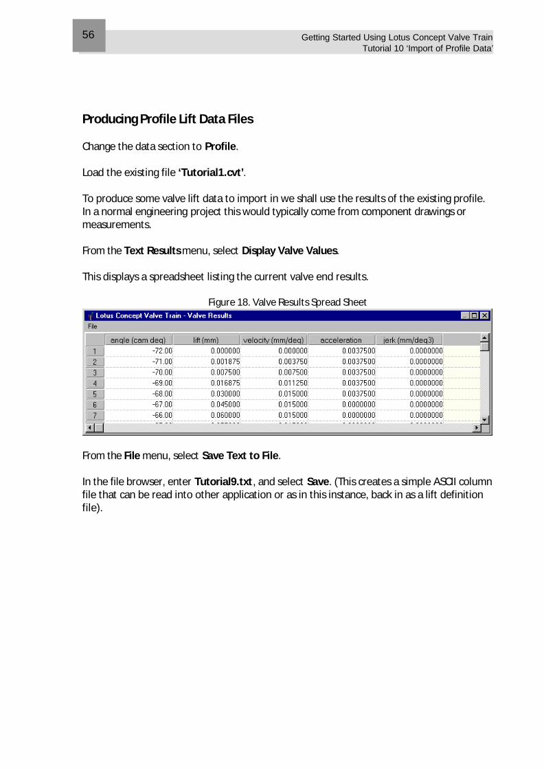
Producing Profile Lift Data Files Change the data section to Profile. Load the existing file ‘Tutorial1.cvt’. To produce some valve lift data to import in we shall use the results of the existing profile. In a normal engineering project this would typically come from component drawings or measurements. From the Text Results menu, select Display Valve Values. This displays a spreadsheet listing the current valve end results.
Figure 18. Valve Results Spread Sheet
From the File menu, select Save Text to File. In the file browser, enter Tutorial9.txt, and select Save. (This creates a simple ASCII column file that can be read into other application or as in this instance, back in as a lift definition file).
Getting Started Using Lotus Concept Valve Train Tutorial 10 ‘Import of Profile Data’
57
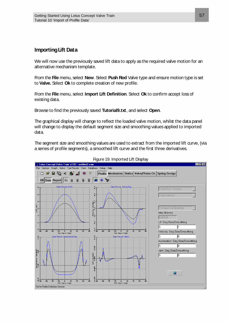
Importing Lift Data We will now use the previously saved lift data to apply as the required valve motion for an alternative mechanism template. From the File menu, select New. Select Push Rod Valve type and ensure motion type is set to Valve. Select Ok to complete creation of new profile. From the File menu, select Import Lift Definition. Select Ok to confirm accept loss of existing data. Browse to find the previously saved Tutorial9.txt, and select Open. The graphical display will change to reflect the loaded valve motion, whilst the data panel will change to display the default segment size and smoothing values applied to imported data. The segment size and smoothing values are used to extract from the imported lift curve, (via a series of profile segments), a smoothed lift curve and the first three derivatives.
Figure 19. Imported Lift Display
Getting Started Using Lotus Concept Valve Train Tutorial 10 ‘Import of Profile Data’
58
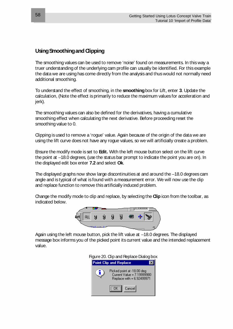
Using Smoothing and Clipping The smoothing values can be used to remove ‘noise’ found on measurements. In this way a truer understanding of the underlying cam profile can usually be identified. For this example the data we are using has come directly from the analysis and thus would not normally need additional smoothing. To understand the effect of smoothing, in the smoothing box for Lift, enter 3. Update the calculation, (Note the effect is primarily to reduce the maximum values for acceleration and jerk). The smoothing values can also be defined for the derivatives, having a cumulative smoothing effect when calculating the next derivative. Before proceeding reset the smoothing value to 0. Clipping is used to remove a ‘rogue’ value. Again because of the origin of the data we are using the lift curve does not have any rogue values, so we will artificially create a problem. Ensure the modify mode is set to Edit. With the left mouse button select on the lift curve the point at –18.0 degrees, (use the status bar prompt to indicate the point you are on). In the displayed edit box enter 7.2 and select Ok. The displayed graphs now show large discontinuities at and around the –18.0 degrees cam angle and is typical of what is found with a measurement error. We will now use the clip and replace function to remove this artificially induced problem. Change the modify mode to clip and replace, by selecting the Clip icon from the toolbar, as indicated below.
Again using the left mouse button, pick the lift value at –18.0 degrees. The displayed message box informs you of the picked point its current value and the intended replacement value.
Figure 20. Clip and Replace Dialog box
Getting Started Using Lotus Concept Valve Train Tutorial 10 ‘Import of Profile Data’
59
Select Ok and the curves will again be smooth, the rogue value having been replaced. Importing Full Profile Data We will now repeat the previous import of the saved lift data, his time we will use not just the lift data but also the velocity, acceleration and jerk values. In this way the program does not need to perform any smoothing or differentiation to obtain the derivatives. From the File menu, select Import Full Profile. Select Ok to confirm accept loss of existing data. Browse to find the previously saved Tutorial9.txt, and select Open. The graphical display will change to reflect the loaded valve motion, whilst the data panel will change to display the default segment size and smoothing values applied to imported full profile data. (Note that the smoothing values are all set to 0 since no smoothing is assumed to be required for a fully defined profile). Uses of Profile Import These sort of techniques are useful for benchmarking existing cam profiles, and for producing the required cam lobe shape for a fully prescribed valve motion, when that valve motion is put through an alternative mechanism geometry. Before moving on to the next tutorial, close the Lotus Concept Valve Train main window, from the File menu select Exit.

Getting Started Using Lotus Concept Valve Train Tutorial 10 ‘Import of Profile Data’
60
Overview To understand the interaction between Lotus Concept Valve Train and other Lotus simulation tools, this tutorial will export a designed cam profile into an existing engine simulation model. This tutorial includes the following sections:
n Opening the Engine Simulation Component, 62
n Loading an Existing Engine Simulation File, 63
n Switching to Lotus Concept Valve Train, 63
n Making the Valve Lift Profile Current, 64
n Viewing the Changes, 65
n Further Data Exchange Opportunities, 66 Note: To complete this tutorial you will need to be licensed to run Lotus Engine Simulation.
12 Tutorial 11. Migration Within Lotus Tools
Getting Started Using Lotus Concept Valve Train Tutorial 11 ‘Migration within Lotus Simulation Tools’
62
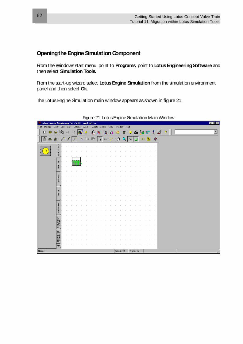
Opening the Engine Simulation Component From the Windows start menu, point to Programs, point to Lotus Engineering Software and then select Simulation Tools. From the start-up wizard select Lotus Engine Simulation from the simulation environment panel and then select Ok. The Lotus Engine Simulation main window appears as shown in figure 21.
Figure 21. Lotus Engine Simulation Main Window
Getting Started Using Lotus Concept Valve Train Tutorial 11 ‘Migration within Lotus Simulation Tools’
63
Loading an Existing Engine Simulation File We will now load one of the default engine simulation models to assist in reviewing the relationship between the software components. From the File menu, select Open. Use the browser to locate tutorial1.sim. Select Open to load the data file. This example file is a very simple single cylinder engine model, having only a cylinder, two valve elements, two port elements and two boundaries, (one inlet one exit). We will use Lotus Concept Valve Train to replace the current valve lift definitions with new valve lift profiles. The current valve lift properties can be examined by selecting the valve element with the left mouse. The property sheet on the right of the display now details the current maximum lift and cam timings for the selected element. Switching to Lotus Concept Valve Train We will now change to the Lotus Concept Valve Train window, From the Tools menu select Lotus Concept Valve Train. As for direct opening of Lotus Concept Valve Train used in the previous tutorials, the application is populated with the default direct acting system, having 8.0 mm maximum lift. Change the maximum valve lift to 10.0 mm, and update the calculation.
Getting Started Using Lotus Concept Valve Train Tutorial 11 ‘Migration within Lotus Simulation Tools’
64
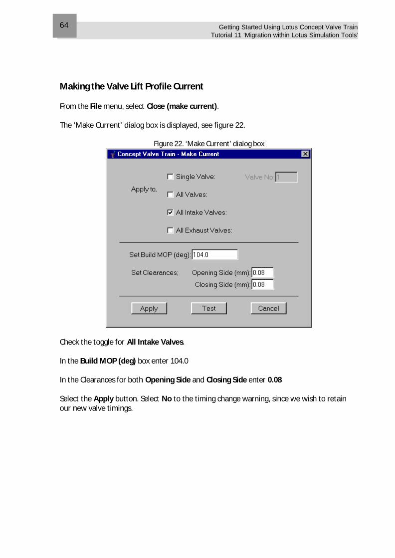
Making the Valve Lift Profile Current From the File menu, select Close (make current). The ‘Make Current’ dialog box is displayed, see figure 22.
Figure 22. ‘Make Current’ dialog box
Check the toggle for All Intake Valves. In the Build MOP (deg) box enter 104.0 In the Clearances for both Opening Side and Closing Side enter 0.08 Select the Apply button. Select No to the timing change warning, since we wish to retain our new valve timings.
Getting Started Using Lotus Concept Valve Train Tutorial 11 ‘Migration within Lotus Simulation Tools’
65
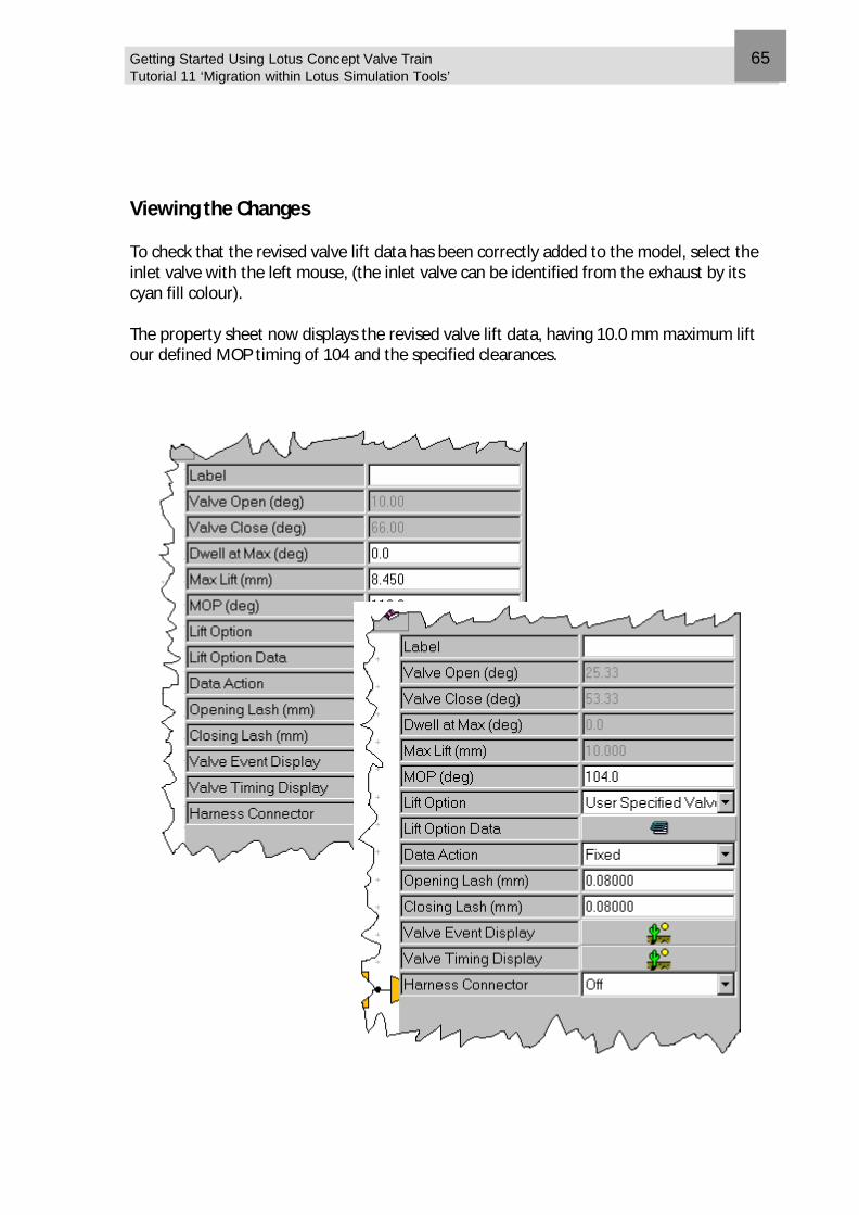
Viewing the Changes To check that the revised valve lift data has been correctly added to the model, select the inlet valve with the left mouse, (the inlet valve can be identified from the exhaust by its cyan fill colour). The property sheet now displays the revised valve lift data, having 10.0 mm maximum lift our defined MOP timing of 104 and the specified clearances.
Getting Started Using Lotus Concept Valve Train Tutorial 11 ‘Migration Within Lotus Simulation Tools’
66
Further Data Exchange Opportunities The method described above is the most likely data exchange route between these two software components. However a number of other routes exist to cover other analysis requirements. Valve to Piston Clearance Select the Inlet Valve component with the right mouse button. From the displayed pop-up menu select Check Valve/Piston Clearance. The valve lift data, (and associated cylinder data) is copied into the Concept Valve Train tool. Only the valve angle and Perpendicular height values now still need to be defined before the valve to piston clearance can be checked. Copy a Valve Elements Lift data into the Valve Train Tool Select the Inlet Valve component with the right mouse button. From the displayed pop-up menu select Load Lift into Concept Valve Train. The valve lift data is copied into the Concept Valve Train tool in exactly the same way as seen in tutorial 9 for an external file.
Overview To assist in identify the differences in designing a cam profile in Lotus Concept Valve Train between the new Bezier Acceleration option and the original polynomial approach, this tutorial will take you through producing both a symmetrical asymmetrical profile. This tutorial includes the following sections:
n Bezier Curves, an overview, 68
n Generating a Symmetrical Bezier Based Cam Profile, 69
n Producing a Valid Symmetrical Bezier Cam Profile, 71
n Editing and Manipulating Bezier Points, 73
n Adding and Deleting Bezier Control Points, 74
n Generating an Asymmetric Bezier Profile, 75
n Producing a Valid Asymmetric Bezier Cam Profile, 76
13 Tutorial 12. Using Bezier Acceleration Curves
Getting Started Using Lotus Concept Valve Train Tutorial 12 ‘Using Bezier Acceleration Curves’
68
Bezier Curves, an Overview The Bezier curve approach to cam profile design is a recognition of the need to provide a fully flexible approach to the shaping of the acceleration curve of a cam profile. Also that this ‘shaping’ is not necessarily a fully quantifiable process in terms of providing direct numerical inputs to achieve the final cam profile. The key difference with Bezier is that the values of the defined points are not actual points on the profile but are control points that shape the curve. The exception to this is the curve end points, which do form points on the profile. The Bezier approach works by defining the profile only in terms of acceleration. The curves for Lift and velocity being calculated via repeated integration and the jerk curve being obtained through differentiation of the Acceleration curve. The acceleration curve is made up of a number of individual Bezier curves, these curves being joined a key points in the profile. This initial version employs six Bezier curves, although other permutations could be possible for future versions. The standard opening and closing ramps are attached to the ends of the first and last Bezier curve to produce the complete cam profile. A Bezier Curve has a minimum of four points, the two end points and an associated control point for each end. The slope of the curve at its end points is set by the angle to its relevant control point, but significant also is the distance between the control point and the end as this controls the ‘strength’ of this directionality. At each Bezier curve junction certain constraints are applied. The first is that they share the same x and y values, secondly that the control points have the same distance from the common end point and that they have the same slope, (albiet mirrored). The shape of a particular Bezier curve can be manipulated by not only moving the two end control points but also by adding additional control points. As with the end control points these points are not actual curve positions but merely points to ‘drag’ and ‘distort’ the actual curve.
Getting Started Using Lotus Concept Valve Train Tutorial 12 ‘Using Bezier Acceleration Curves’
69
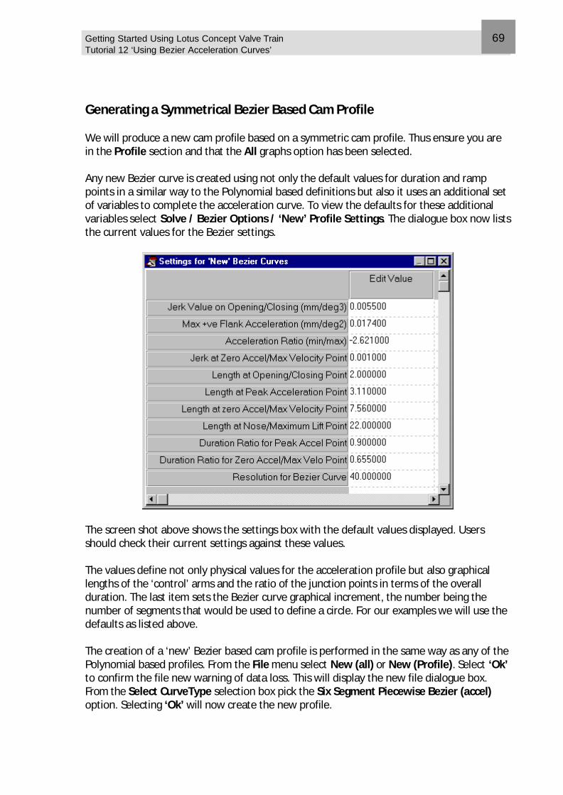
Generating a Symmetrical Bezier Based Cam Profile We will produce a new cam profile based on a symmetric cam profile. Thus ensure you are in the Profile section and that the All graphs option has been selected. Any new Bezier curve is created using not only the default values for duration and ramp points in a similar way to the Polynomial based definitions but also it uses an additional set of variables to complete the acceleration curve. To view the defaults for these additional variables select Solve / Bezier Options / ‘New’ Profile Settings. The dialogue box now lists the current values for the Bezier settings.
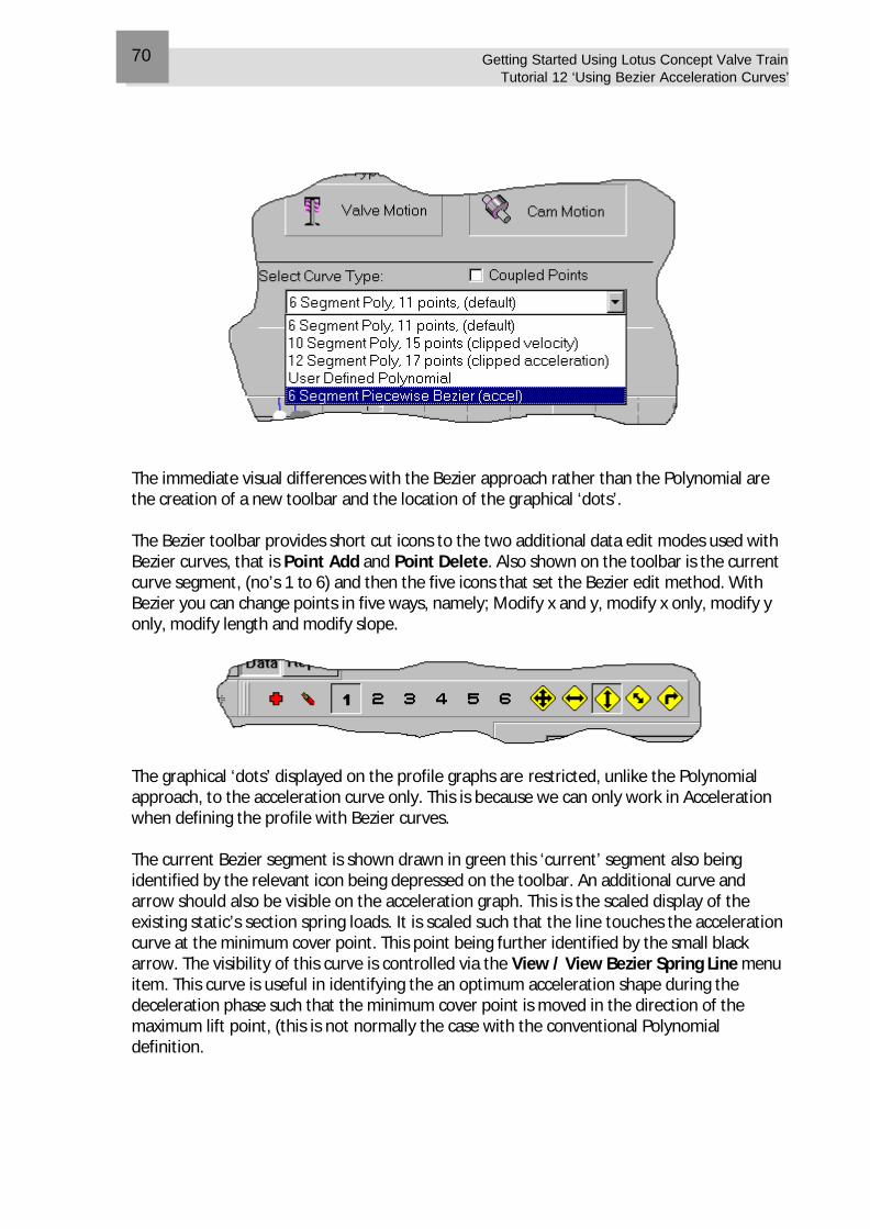
The screen shot above shows the settings box with the default values displayed. Users should check their current settings against these values. The values define not only physical values for the acceleration profile but also graphical lengths of the ‘control’ arms and the ratio of the junction points in terms of the overall duration. The last item sets the Bezier curve graphical increment, the number being the number of segments that would be used to define a circle. For our examples we will use the defaults as listed above. The creation of a ‘new’ Bezier based cam profile is performed in the same way as any of the Polynomial based profiles. From the File menu select New (all) or New (Profile). Select ‘Ok’ to confirm the file new warning of data loss. This will display the new file dialogue box. From the Select CurveType selection box pick the Six Segment Piecewise Bezier (accel) option. Selecting ‘Ok’ will now create the new profile.
Getting Started Using Lotus Concept Valve Train Tutorial 12 ‘Using Bezier Acceleration Curves’
70
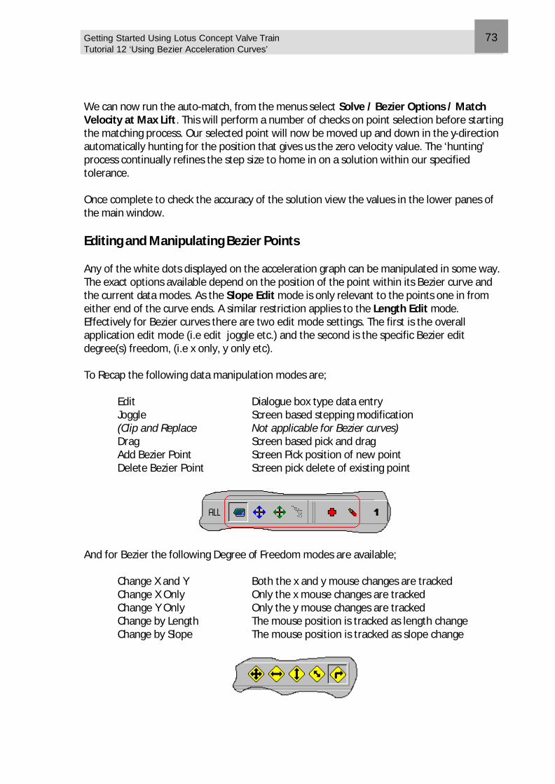
The immediate visual differences with the Bezier approach rather than the Polynomial are the creation of a new toolbar and the location of the graphical ‘dots’. The Bezier toolbar provides short cut icons to the two additional data edit modes used with Bezier curves, that is Point Add and Point Delete. Also shown on the toolbar is the current curve segment, (no’s 1 to 6) and then the five icons that set the Bezier edit method. With Bezier you can change points in five ways, namely; Modify x and y, modify x only, modify y only, modify length and modify slope.
The graphical ‘dots’ displayed on the profile graphs are restricted, unlike the Polynomial approach, to the acceleration curve only. This is because we can only work in Acceleration when defining the profile with Bezier curves. The current Bezier segment is shown drawn in green this ‘current’ segment also being identified by the relevant icon being depressed on the toolbar. An additional curve and arrow should also be visible on the acceleration graph. This is the scaled display of the existing static’s section spring loads. It is scaled such that the line touches the acceleration curve at the minimum cover point. This point being further identified by the small black arrow. The visibility of this curve is controlled via the View / View Bezier Spring Line menu item. This curve is useful in identifying the an optimum acceleration shape during the deceleration phase such that the minimum cover point is moved in the direction of the maximum lift point, (this is not normally the case with the conventional Polynomial definition.
Getting Started Using Lotus Concept Valve Train Tutorial 12 ‘Using Bezier Acceleration Curves’
71
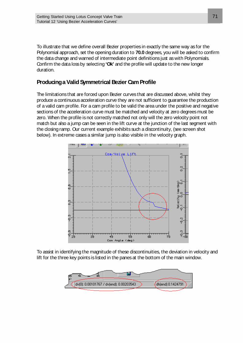
To illustrate that we define overall Bezier properties in exactly the same way as for the Polynomial approach, set the opening duration to 70.0 degrees, you will be asked to confirm the data change and warned of intermediate point definitions just as with Polynomials. Confirm the data loss by selecting ‘Ok’ and the profile will update to the new longer duration. Producing a Valid Symmetrical Bezier Cam Profile The limitations that are forced upon Bezier curves that are discussed above, whilst they produce a continuous acceleration curve they are not sufficient to guarantee the production of a valid cam profile. For a cam profile to be valid the area under the positive and negative sections of the acceleration curve must be matched and velocity at zero degrees must be zero. When the profile is not correctly matched not only will the zero velocity point not match but also a jump can be seen in the lift curve at the junction of the last segment with the closing ramp. Our current example exhibits such a discontinuity, (see screen shot below). In extreme cases a similar jump is also visible in the velocity graph.
To assist in identifying the magnitude of these discontinuities, the deviation in velocity and lift for the three key points is listed in the panes at the bottom of the main window.
Getting Started Using Lotus Concept Valve Train Tutorial 12 ‘Using Bezier Acceleration Curves’
72
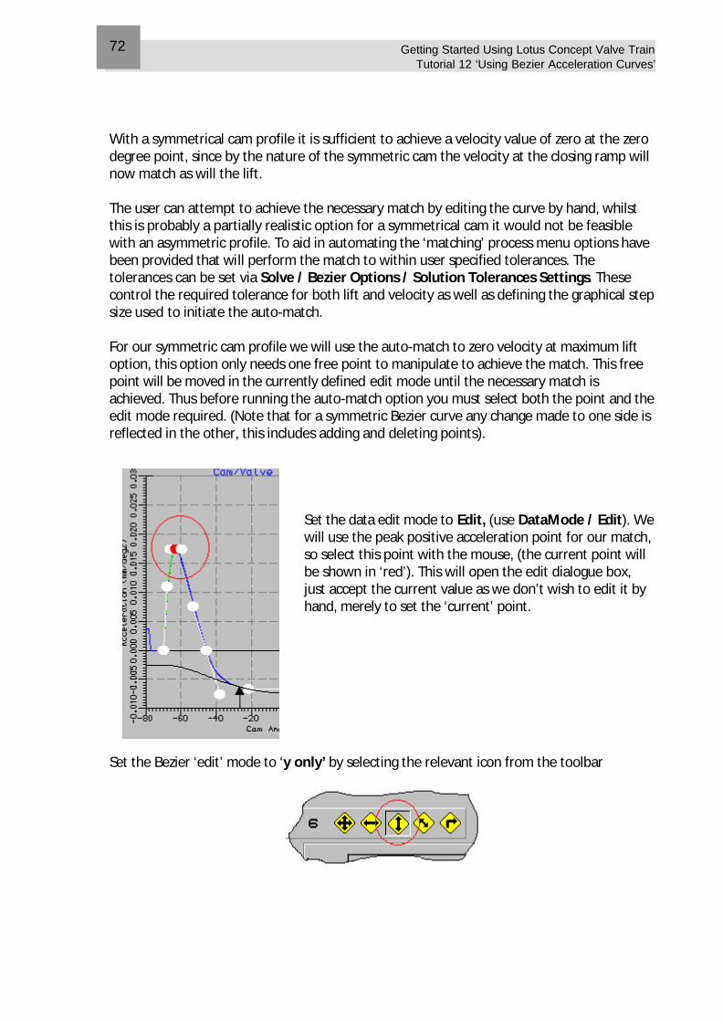
With a symmetrical cam profile it is sufficient to achieve a velocity value of zero at the zero degree point, since by the nature of the symmetric cam the velocity at the closing ramp will now match as will the lift. The user can attempt to achieve the necessary match by editing the curve by hand, whilst this is probably a partially realistic option for a symmetrical cam it would not be feasible with an asymmetric profile. To aid in automating the ‘matching’ process menu options have been provided that will perform the match to within user specified tolerances. The tolerances can be set via Solve / Bezier Options / Solution Tolerances Settings. These control the required tolerance for both lift and velocity as well as defining the graphical step size used to initiate the auto-match. For our symmetric cam profile we will use the auto-match to zero velocity at maximum lift option, this option only needs one free point to manipulate to achieve the match. This free point will be moved in the currently defined edit mode until the necessary match is achieved. Thus before running the auto-match option you must select both the point and the edit mode required. (Note that for a symmetric Bezier curve any change made to one side is reflected in the other, this includes adding and deleting points).
Set the data edit mode to Edit, (use DataMode / Edit). We will use the peak positive acceleration point for our match, so select this point with the mouse, (the current point will be shown in ‘red’). This will open the edit dialogue box, just accept the current value as we don’t wish to edit it by hand, merely to set the ‘current’ point.
Set the Bezier ‘edit’ mode to ‘y only’ by selecting the relevant icon from the toolbar
Getting Started Using Lotus Concept Valve Train Tutorial 12 ‘Using Bezier Acceleration Curves’
73
We can now run the auto-match, from the menus select Solve / Bezier Options / Match Velocity at Max Lift. This will perform a number of checks on point selection before starting the matching process. Our selected point will now be moved up and down in the y-direction automatically hunting for the position that gives us the zero velocity value. The ‘hunting’ process continually refines the step size to home in on a solution within our specified tolerance. Once complete to check the accuracy of the solution view the values in the lower panes of the main window. Editing and Manipulating Bezier Points Any of the white dots displayed on the acceleration graph can be manipulated in some way. The exact options available depend on the position of the point within its Bezier curve and the current data modes. As the Slope Edit mode is only relevant to the points one in from either end of the curve ends. A similar restriction applies to the Length Edit mode. Effectively for Bezier curves there are two edit mode settings. The first is the overall application edit mode (i.e edit joggle etc.) and the second is the specific Bezier edit degree(s) freedom, (i.e x only, y only etc). To Recap the following data manipulation modes are; Edit Dialogue box type data entry Joggle Screen based stepping modification (Clip and Replace Not applicable for Bezier curves) Drag Screen based pick and drag Add Bezier Point Screen Pick position of new point Delete Bezier Point Screen pick delete of existing point
And for Bezier the following Degree of Freedom modes are available; Change X and Y Both the x and y mouse changes are tracked Change X Only Only the x mouse changes are tracked Change Y Only Only the y mouse changes are tracked Change by Length The mouse position is tracked as length change Change by Slope The mouse position is tracked as slope change
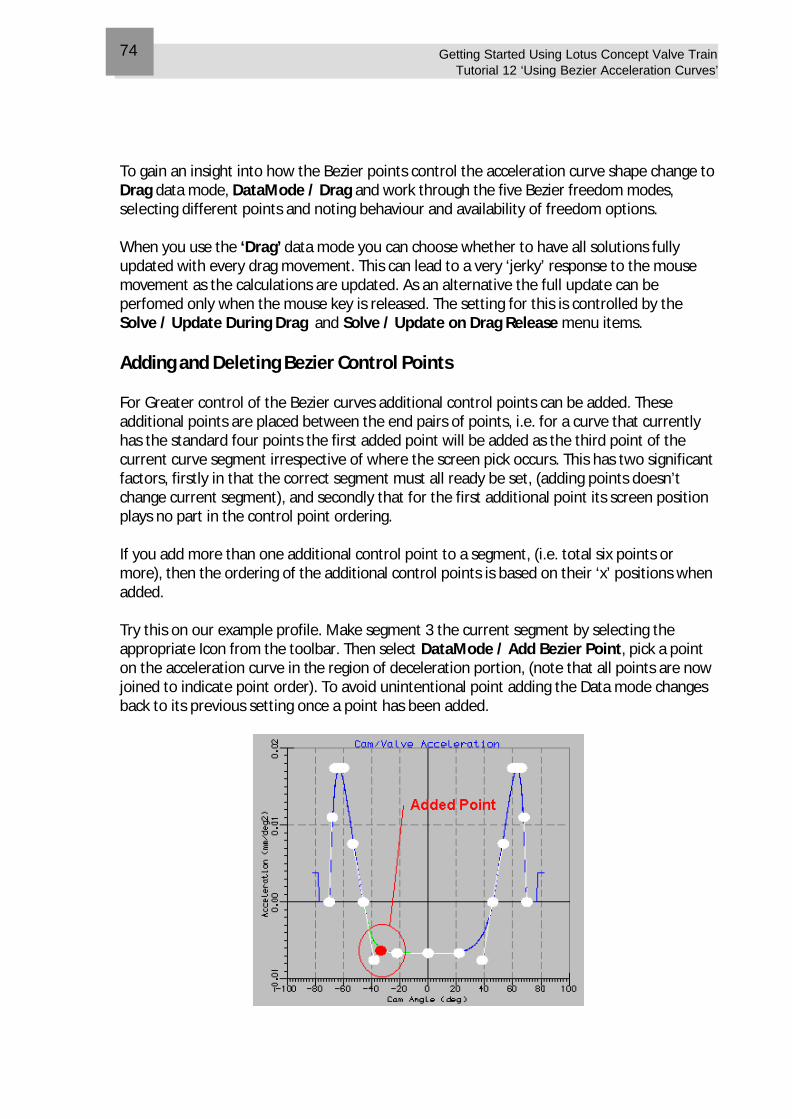
Getting Started Using Lotus Concept Valve Train Tutorial 12 ‘Using Bezier Acceleration Curves’
74
To gain an insight into how the Bezier points control the acceleration curve shape change to Drag data mode, DataMode / Drag and work through the five Bezier freedom modes, selecting different points and noting behaviour and availability of freedom options. When you use the ‘Drag’ data mode you can choose whether to have all solutions fully updated with every drag movement. This can lead to a very ‘jerky’ response to the mouse movement as the calculations are updated. As an alternative the full update can be perfomed only when the mouse key is released. The setting for this is controlled by the Solve / Update During Drag and Solve / Update on Drag Release menu items. Adding and Deleting Bezier Control Points For Greater control of the Bezier curves additional control points can be added. These additional points are placed between the end pairs of points, i.e. for a curve that currently has the standard four points the first added point will be added as the third point of the current curve segment irrespective of where the screen pick occurs. This has two significant factors, firstly in that the correct segment must all ready be set, (adding points doesn’t change current segment), and secondly that for the first additional point its screen position plays no part in the control point ordering. If you add more than one additional control point to a segment, (i.e. total six points or more), then the ordering of the additional control points is based on their ‘x’ positions when added. Try this on our example profile. Make segment 3 the current segment by selecting the appropriate Icon from the toolbar. Then select DataMode / Add Bezier Point, pick a point on the acceleration curve in the region of deceleration portion, (note that all points are now joined to indicate point order). To avoid unintentional point adding the Data mode changes back to its previous setting once a point has been added.
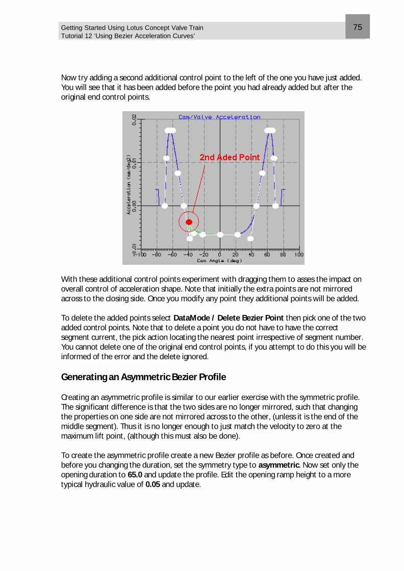
Getting Started Using Lotus Concept Valve Train Tutorial 12 ‘Using Bezier Acceleration Curves’
75
Now try adding a second additional control point to the left of the one you have just added. You will see that it has been added before the point you had already added but after the original end control points.
With these additional control points experiment with dragging them to asses the impact on overall control of acceleration shape. Note that initially the extra points are not mirrored across to the closing side. Once you modify any point they additional points will be added. To delete the added points select DataMode / Delete Bezier Point then pick one of the two added control points. Note that to delete a point you do not have to have the correct segment current, the pick action locating the nearest point irrespective of segment number. You cannot delete one of the original end control points, if you attempt to do this you will be informed of the error and the delete ignored. Generating an Asymmetric Bezier Profile Creating an asymmetric profile is similar to our earlier exercise with the symmetric profile. The significant difference is that the two sides are no longer mirrored, such that changing the properties on one side are not mirrored across to the other, (unless it is the end of the middle segment). Thus it is no longer enough to just match the velocity to zero at the maximum lift point, (although this must also be done). To create the asymmetric profile create a new Bezier profile as before. Once created and before you changing the duration, set the symmetry type to asymmetric. Now set only the opening duration to 65.0 and update the profile. Edit the opening ramp height to a more typical hydraulic value of 0.05 and update.
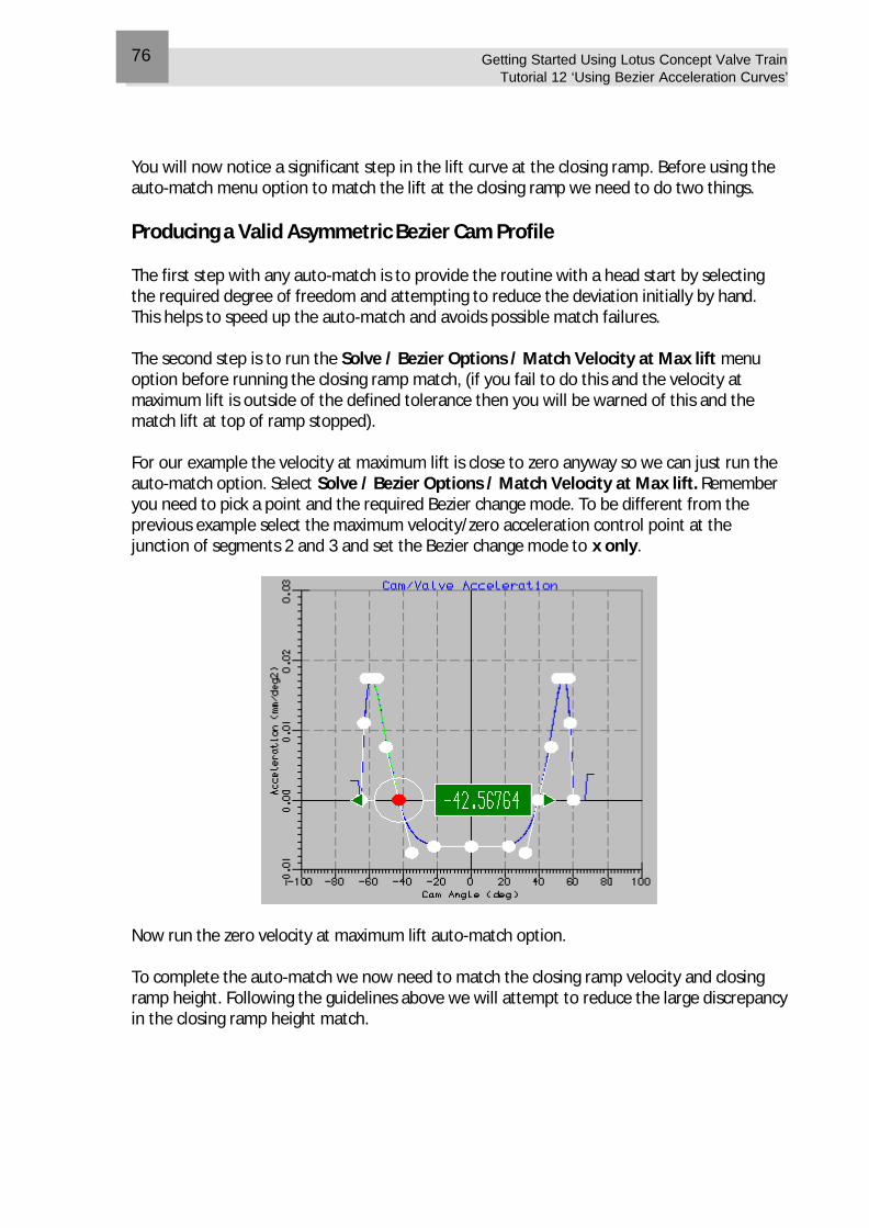
Getting Started Using Lotus Concept Valve Train Tutorial 12 ‘Using Bezier Acceleration Curves’
76
You will now notice a significant step in the lift curve at the closing ramp. Before using the auto-match menu option to match the lift at the closing ramp we need to do two things. Producing a Valid Asymmetric Bezier Cam Profile The first step with any auto-match is to provide the routine with a head start by selecting the required degree of freedom and attempting to reduce the deviation initially by hand. This helps to speed up the auto-match and avoids possible match failures. The second step is to run the Solve / Bezier Options / Match Velocity at Max lift menu option before running the closing ramp match, (if you fail to do this and the velocity at maximum lift is outside of the defined tolerance then you will be warned of this and the match lift at top of ramp stopped). For our example the velocity at maximum lift is close to zero anyway so we can just run the auto-match option. Select Solve / Bezier Options / Match Velocity at Max lift. Remember you need to pick a point and the required Bezier change mode. To be different from the previous example select the maximum velocity/zero acceleration control point at the junction of segments 2 and 3 and set the Bezier change mode to x only.
Now run the zero velocity at maximum lift auto-match option. To complete the auto-match we now need to match the closing ramp velocity and closing ramp height. Following the guidelines above we will attempt to reduce the large discrepancy in the closing ramp height match.
Getting Started Using Lotus Concept Valve Train Tutorial 12 ‘Using Bezier Acceleration Curves’
77
To assist the ramp height match we will drag the height of the peak acceleration control point at the junction between segments 5 and 6. Remember that once you have matched the velocity at maximum lift you must avoid changing control points on the opening side or indeed, on the closing side at the junction between segment 3 and 4, since this also effects the opening side. We will also drag the zero acceleration point at the junction of segments 4 and 5. Try to reduce the deviations as much as possible. You should find that you need to drag the peak acceleration point up to around 0.037 and the zero acceleration point to about 46.0
You are now in a position to run the auto-match, select Solve / Bezier Options / Match Lift at Closing Ramp. This will open a dialogue box through which you define the two points you wish to move to match and the freedom degree for each.
Getting Started Using Lotus Concept Valve Train Tutorial 12 ‘Using Bezier Acceleration Curves’
78
For our example we will select the first point to be Point No 1 on Curve 5 and to allow the change mode to be X only. The second point set as Point No. 1 on Curve 6 and o allow the change mode to be Y only. Once set select ‘Ok’ and this will start the auto match process. The final matched profile is shown below.
The highly asymmetric nature of this profile would not be typical but is intended to illustrate the process of matching highly unequal profile halves. As with all cam profile designs, irrespective of their maths origins, the profile should be checked for overall acceptable results. This particular example would almost certainly not be due to its high acceleration and jerk values.
Overview This tutorial introduces the dynamic spring module. The dynamic spring module auto-generates a multi-mass equivalent model of the currently defined kinematic system. Dynamic analysis of this lumped mass model provides insight into the dynamic behaviour of the valve spring and valve train components. This tutorial includes the following sections:
n Dynamic Analysis, an overview, 80
n Changing to the Dynamics Module, 81
n Dynamic Model Types, 82
n Auto-Creating the Complete Model, 82
n Auto-Updating Model Parts, 83
n Selecting and Editing Mass Properties, 84
n Selecting and Editing Link Properties, 85
n ‘Special’ Element Properties, 86
n Defining the Profile, 87
n Defining Gas Loads, 87
n Running the Analysis, 88
n Controlling the Results Screen Display, 90
n Listing Overall Results, 92
14 Tutorial 13. The Dynamic Spring Module
Getting Started Using Lotus Concept Valve Train Tutorial 13 ‘The Dynamic Spring Module’
80
Dynamic Analysis, an Overview The Dynamic analysis module allows the dynamic behaviour of the valve spring and associated valve train parts to be analysed. The analysis uses an equivalent lumped mass representation of the valve and valve train system. The spring is defined as a series of masses and springs. Whilst additional masses are used to represent the retainer, valve head, and tappet parts. Currently rockers and finger based systems use the tappet mass to represent a single effective mass of the valve train system. The creation of the dynamics model can be performed in a semi-automatic manner using the data values in the kinematic module and the defaults in the Adams/Engine data section. This can be used to create both mechanical, hydraulic and cam profile switching (CPS) tappet models and single springs, double springs or gas springs models. Individual model elements can be selected and their properties listed for display and editing. The cam profile definition can be the current profile or a saved list. The model can include external gas forces that vary as a function of crank angle applied to the valve head from the cylinder side and the port side. The model can also be solved directly with the engine simulation program as a ‘co-simulation’ to link dynamic valve motion and calculated gas forces. The model can be run at a constant speed or a series of speed steps or a steadily increasing speed run. The model solution is animated on screen during the analysis to indicate forces and displacements in the system. Post analysis overall summary results such as peak seating force, spring surge and maximum valve bounce can be displayed both numerically and graphically. We will start this tutorial using the default direct acting profile and mechanism data. Select File / New (all) and select Direct Acting and Cam Motion and 6 Segment Poly.
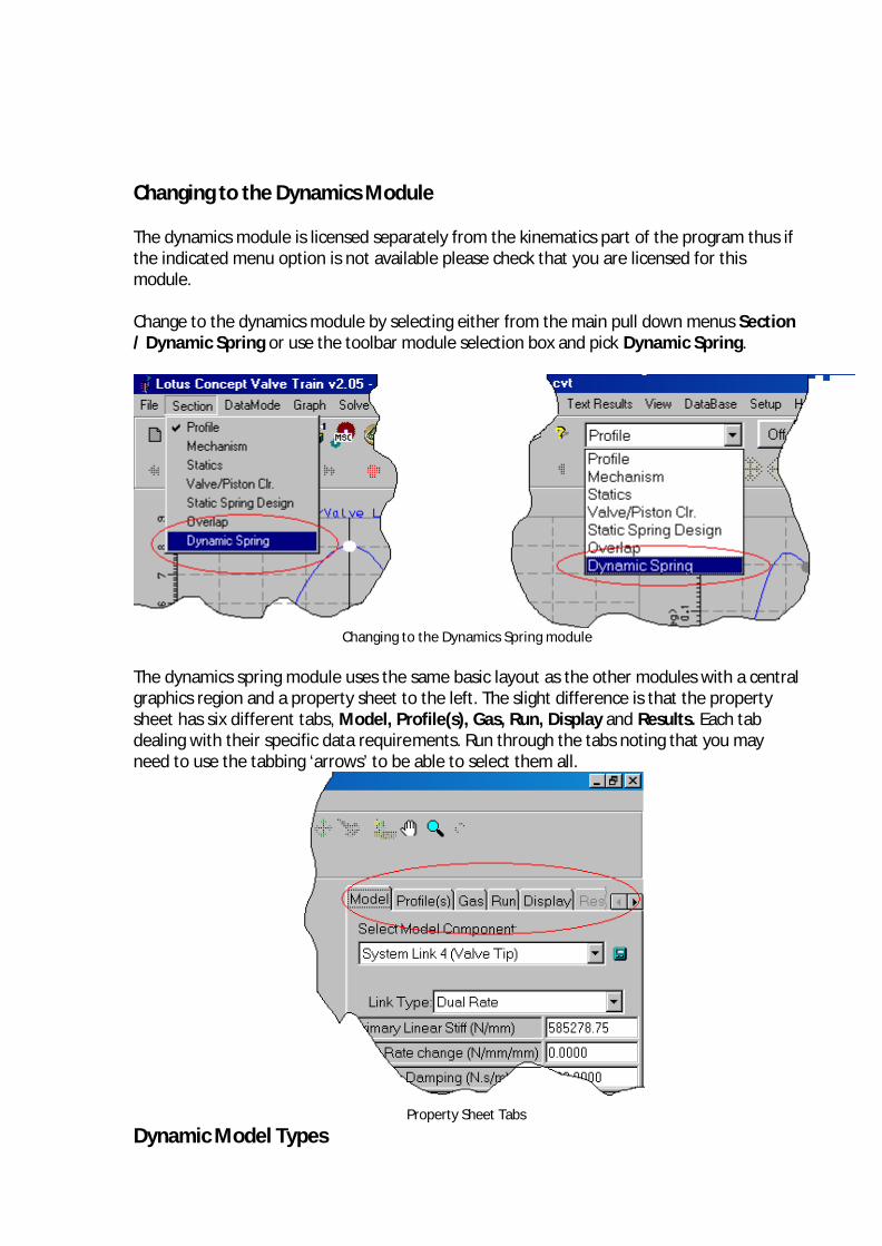
Changing to the Dynamics Module The dynamics module is licensed separately from the kinematics part of the program thus if the indicated menu option is not available please check that you are licensed for this module. Change to the dynamics module by selecting either from the main pull down menus Section / Dynamic Spring or use the toolbar module selection box and pick Dynamic Spring.
Changing to the Dynamics Spring module The dynamics spring module uses the same basic layout as the other modules with a central graphics region and a property sheet to the left. The slight difference is that the property sheet has six different tabs, Model, Profile(s), Gas, Run, Display and Results. Each tab dealing with their specific data requirements. Run through the tabs noting that you may need to use the tabbing ‘arrows’ to be able to select them all.
Property Sheet Tabs
Dynamic Model Types
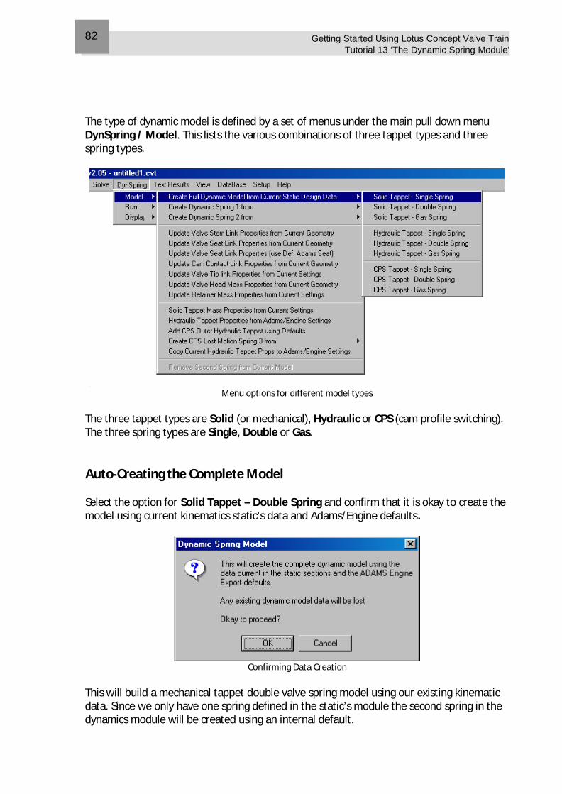
Getting Started Using Lotus Concept Valve Train Tutorial 13 ‘The Dynamic Spring Module’
82
The type of dynamic model is defined by a set of menus under the main pull down menu DynSpring / Model. This lists the various combinations of three tappet types and three spring types.
Menu options for different model types
The three tappet types are Solid (or mechanical), Hydraulic or CPS (cam profile switching). The three spring types are Single, Double or Gas. Auto-Creating the Complete Model Select the option for Solid Tappet – Double Spring and confirm that it is okay to create the model using current kinematics static’s data and Adams/Engine defaults.
Confirming Data Creation
This will build a mechanical tappet double valve spring model using our existing kinematic data. Since we only have one spring defined in the static’s module the second spring in the dynamics module will be created using an internal default.
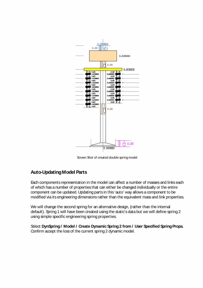
Screen Shot of created double spring model
Auto-Updating Model Parts Each components representation in the model can affect a number of masses and links each of which has a number of properties that can either be changed individually or the entire component can be updated. Updating parts in this ‘auto’ way allows a component to be modified via its engineering dimensions rather than the equivalent mass and link properties. We will change the second spring for an alternative design, (rather than the internal default). Spring 1 will have been created using the static’s data but we will define spring 2 using simple specific engineering spring properties. Select DynSpring / Model / Create Dynamic Spring 2 from / User Specified Spring Props. Confirm accept the loss of the current spring 2 dynamic model.
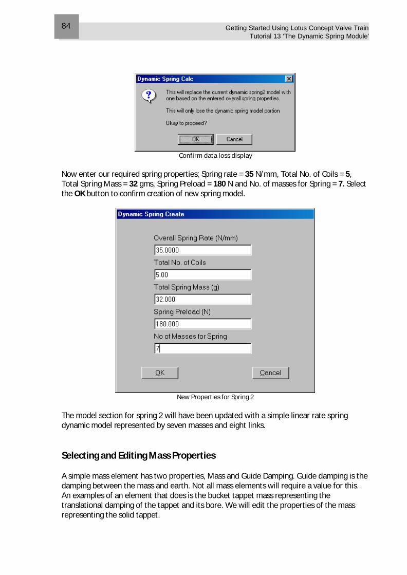
Getting Started Using Lotus Concept Valve Train Tutorial 13 ‘The Dynamic Spring Module’
84
Confirm data loss display
Now enter our required spring properties; Spring rate = 35 N/mm, Total No. of Coils = 5, Total Spring Mass = 32 gms, Spring Preload = 180 N and No. of masses for Spring = 7. Select the OK button to confirm creation of new spring model.
New Properties for Spring 2
The model section for spring 2 will have been updated with a simple linear rate spring dynamic model represented by seven masses and eight links. Selecting and Editing Mass Properties A simple mass element has two properties, Mass and Guide Damping. Guide damping is the damping between the mass and earth. Not all mass elements will require a value for this. An examples of an element that does is the bucket tappet mass representing the translational damping of the tappet and its bore. We will edit the properties of the mass representing the solid tappet.
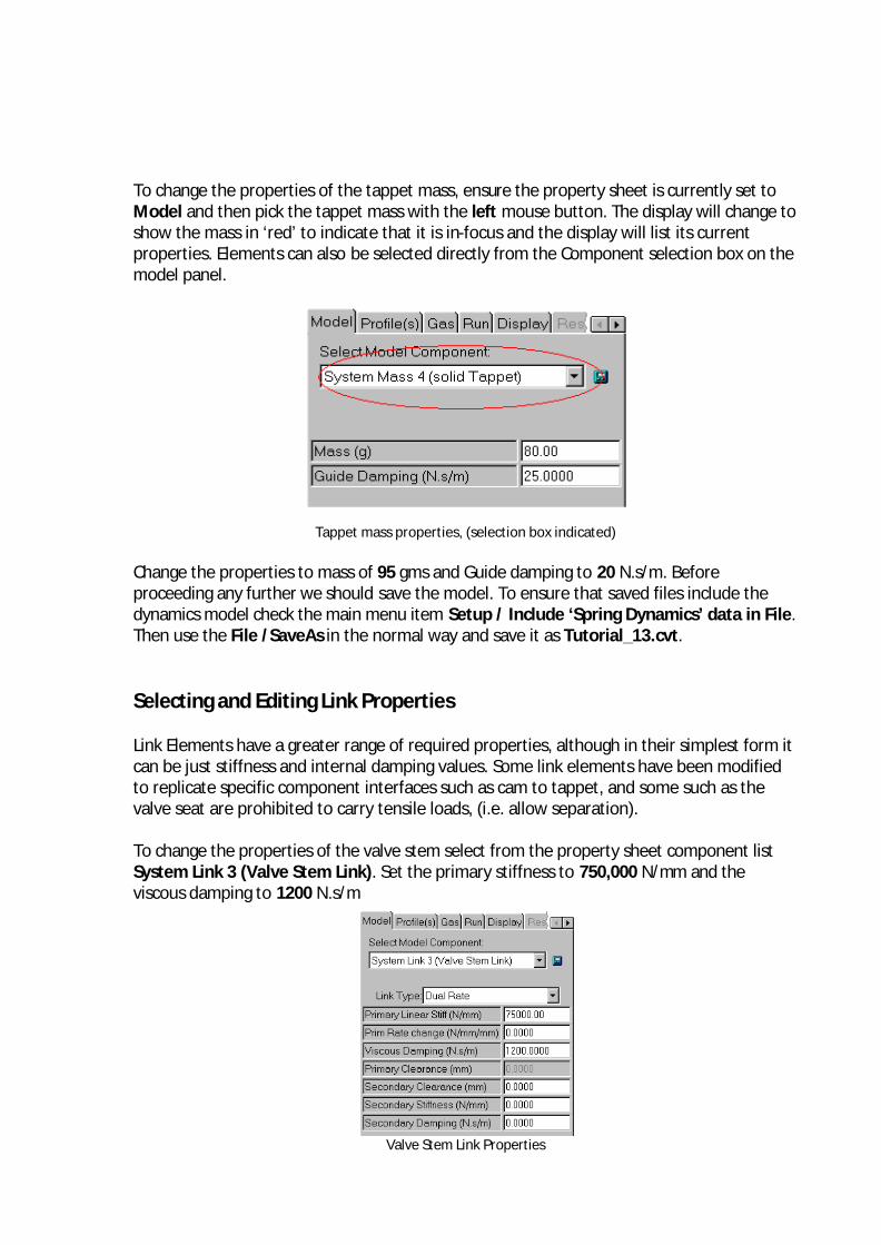
To change the properties of the tappet mass, ensure the property sheet is currently set to Model and then pick the tappet mass with the left mouse button. The display will change to show the mass in ‘red’ to indicate that it is in-focus and the display will list its current properties. Elements can also be selected directly from the Component selection box on the model panel.
Tappet mass properties, (selection box indicated)
Change the properties to mass of 95 gms and Guide damping to 20 N.s/m. Before proceeding any further we should save the model. To ensure that saved files include the dynamics model check the main menu item Setup / Include ‘Spring Dynamics’ data in File. Then use the File /SaveAs in the normal way and save it as Tutorial_13.cvt. Selecting and Editing Link Properties Link Elements have a greater range of required properties, although in their simplest form it can be just stiffness and internal damping values. Some link elements have been modified to replicate specific component interfaces such as cam to tappet, and some such as the valve seat are prohibited to carry tensile loads, (i.e. allow separation). To change the properties of the valve stem select from the property sheet component list System Link 3 (Valve Stem Link). Set the primary stiffness to 750,000 N/mm and the viscous damping to 1200 N.s/m
Valve Stem Link Properties
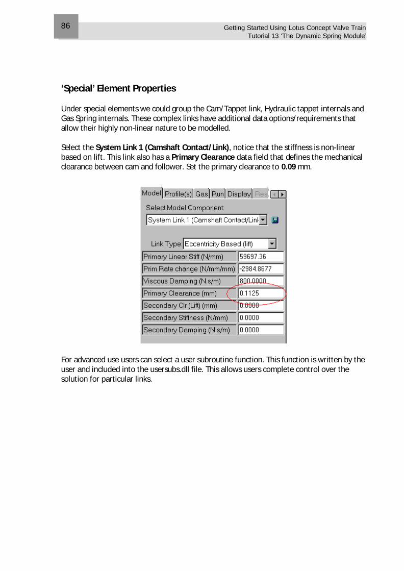
Getting Started Using Lotus Concept Valve Train Tutorial 13 ‘The Dynamic Spring Module’
86
‘Special’ Element Properties Under special elements we could group the Cam/Tappet link, Hydraulic tappet internals and Gas Spring internals. These complex links have additional data options/requirements that allow their highly non-linear nature to be modelled. Select the System Link 1 (Camshaft Contact/Link), notice that the stiffness is non-linear based on lift. This link also has a Primary Clearance data field that defines the mechanical clearance between cam and follower. Set the primary clearance to 0.09 mm.
For advanced use users can select a user subroutine function. This function is written by the user and included into the usersubs.dll file. This allows users complete control over the solution for particular links.
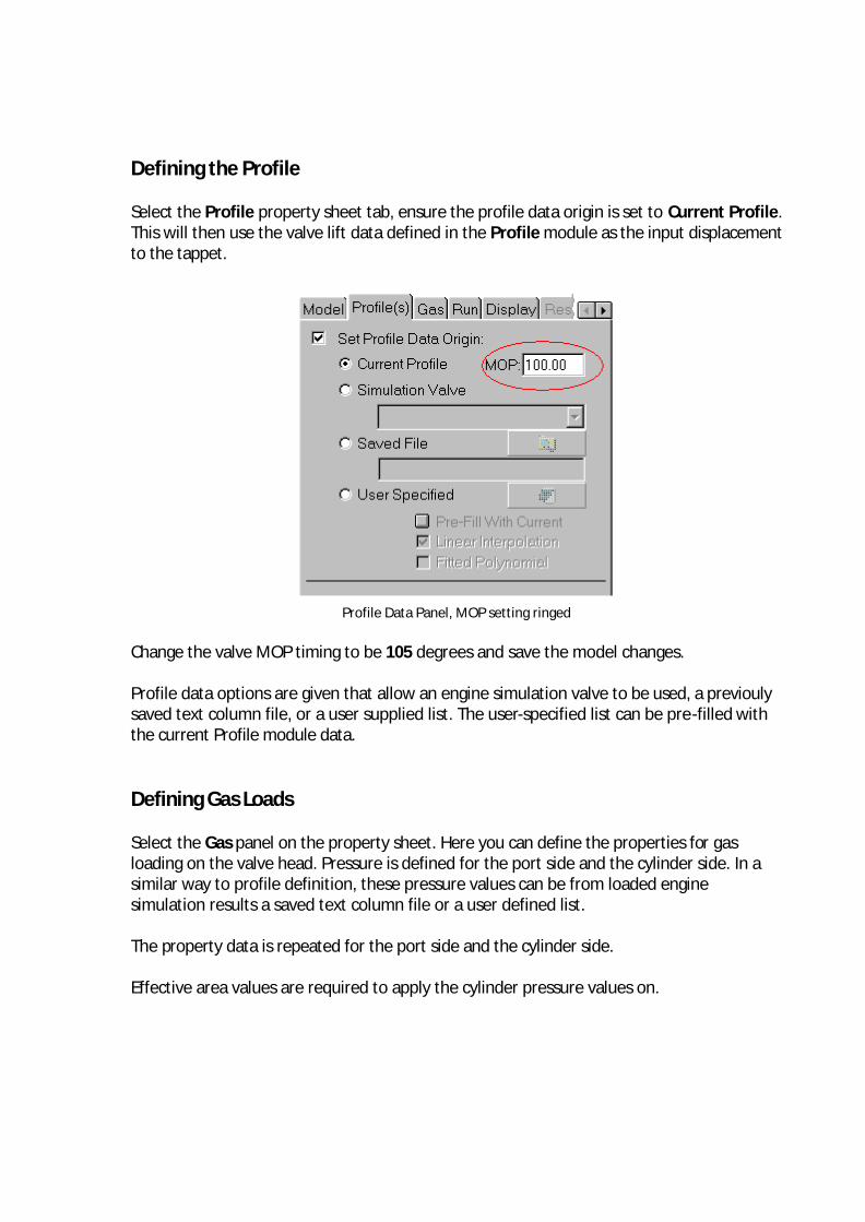
Defining the Profile Select the Profile property sheet tab, ensure the profile data origin is set to Current Profile. This will then use the valve lift data defined in the Profile module as the input displacement to the tappet.
Profile Data Panel, MOP setting ringed
Change the valve MOP timing to be 105 degrees and save the model changes. Profile data options are given that allow an engine simulation valve to be used, a previouly saved text column file, or a user supplied list. The user-specified list can be pre-filled with the current Profile module data. Defining Gas Loads Select the Gas panel on the property sheet. Here you can define the properties for gas loading on the valve head. Pressure is defined for the port side and the cylinder side. In a similar way to profile definition, these pressure values can be from loaded engine simulation results a saved text column file or a user defined list. The property data is repeated for the port side and the cylinder side. Effective area values are required to apply the cylinder pressure values on.
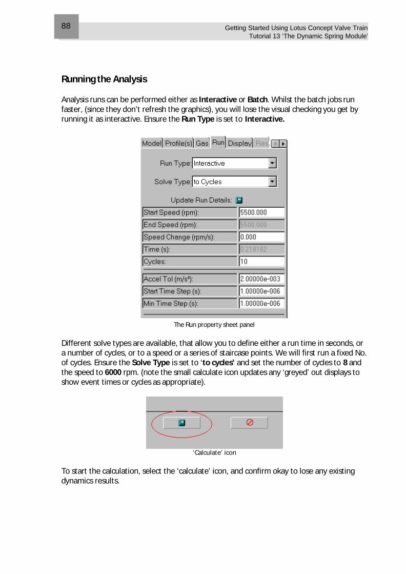
Getting Started Using Lotus Concept Valve Train Tutorial 13 ‘The Dynamic Spring Module’
88
Running the Analysis Analysis runs can be performed either as Interactive or Batch. Whilst the batch jobs run faster, (since they don’t refresh the graphics), you will lose the visual checking you get by running it as interactive. Ensure the Run Type is set to Interactive.
The Run property sheet panel
Different solve types are available, that allow you to define either a run time in seconds, or a number of cycles, or to a speed or a series of staircase points. We will first run a fixed No. of cycles. Ensure the Solve Type is set to ‘to cycles’ and set the number of cycles to 8 and the speed to 6000 rpm. (note the small calculate icon updates any ‘greyed’ out displays to show event times or cycles as appropriate).
‘Calculate’ icon
To start the calculation, select the ‘calculate’ icon, and confirm okay to lose any existing dynamics results.
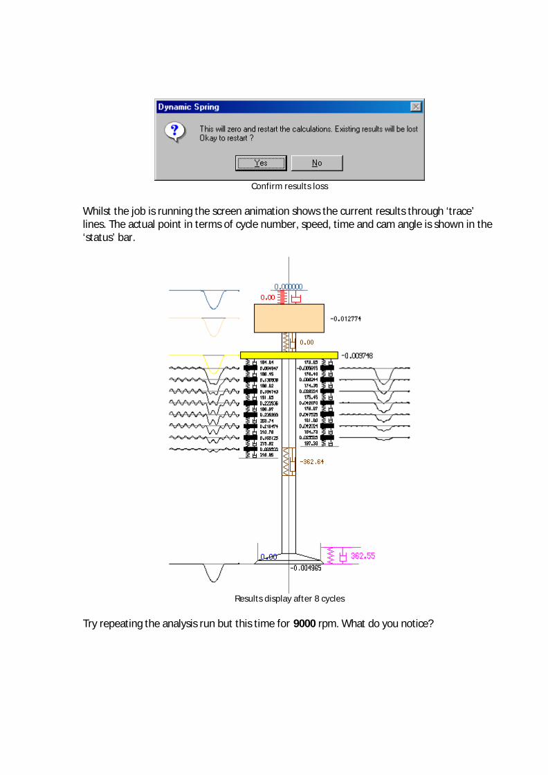
Confirm results loss
Whilst the job is running the screen animation shows the current results through ‘trace’ lines. The actual point in terms of cycle number, speed, time and cam angle is shown in the ‘status’ bar.
Results display after 8 cycles
Try repeating the analysis run but this time for 9000 rpm. What do you notice?
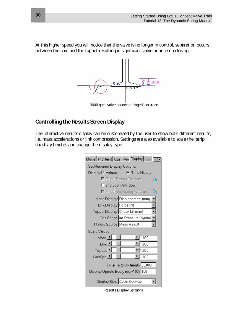
Getting Started Using Lotus Concept Valve Train Tutorial 13 ‘The Dynamic Spring Module’
90
At this higher speed you will notice that the valve is no longer in control, separation occurs between the cam and the tappet resulting in significant valve bounce on closing.
9000 rpm, valve bounced ‘ringed’ on trace
Controlling the Results Screen Display The interactive results display can be customised by the user to show both different results, i.e. mass accelerations or link compression. Settings are also available to scale the ‘strip charts’ y-heights and change the display type.
Results Display Settings
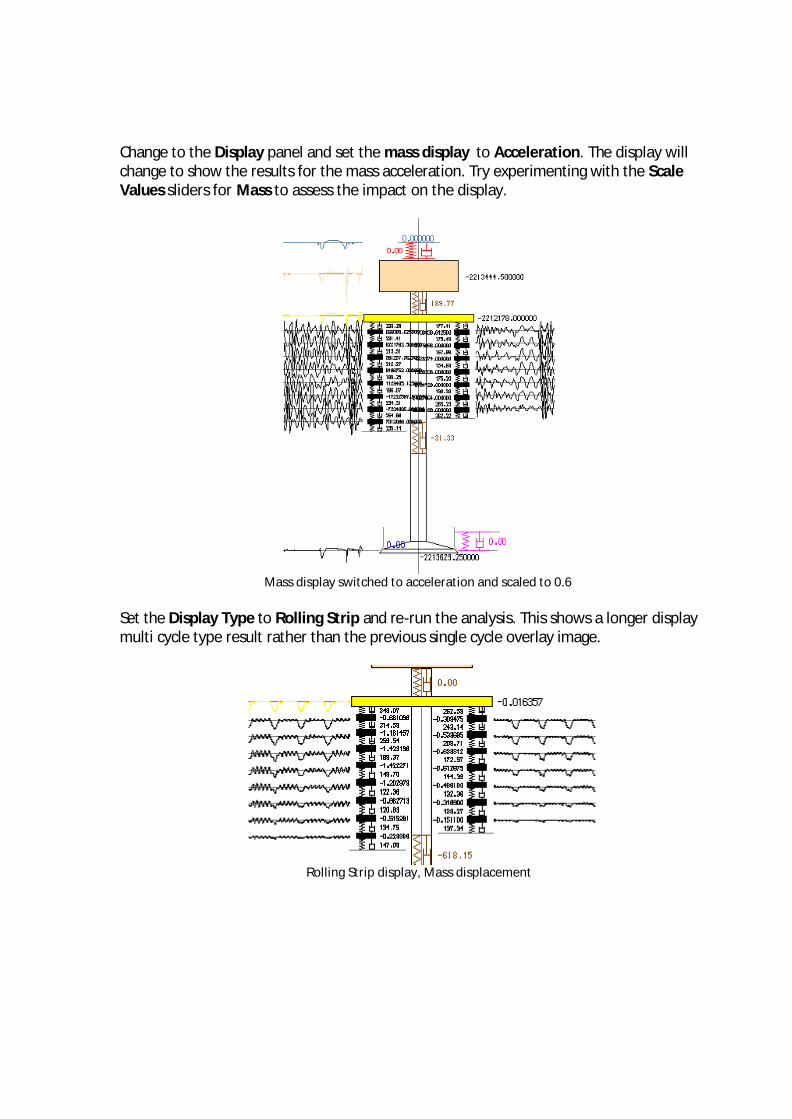
Change to the Display panel and set the mass display to Acceleration. The display will change to show the results for the mass acceleration. Try experimenting with the Scale Values sliders for Mass to assess the impact on the display.
Mass display switched to acceleration and scaled to 0.6
Set the Display Type to Rolling Strip and re-run the analysis. This shows a longer display multi cycle type result rather than the previous single cycle overlay image.
Rolling Strip display, Mass displacement
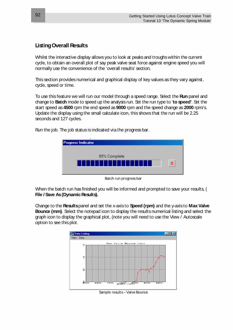
Getting Started Using Lotus Concept Valve Train Tutorial 13 ‘The Dynamic Spring Module’
92
Listing Overall Results Whilst the interactive display allows you to look at peaks and troughs within the current cycle, to obtain an overall plot of say peak valve seat force against engine speed you will normally use the convenience of the ‘overall results’ section. This section provides numerical and graphical display of key values as they vary against, cycle, speed or time. To use this feature we will run our model through a speed range. Select the Run panel and change to Batch mode to speed up the analysis run. Set the run type to ‘to speed’. Set the start speed as 4500 rpm the end speed as 9000 rpm and the speed change as 2000 rpm/s. Update the display using the small calculate icon, this shows that the run will be 2.25 seconds and 127 cycles. Run the job. The job status is indicated via the progress bar.
Batch run progress bar
When the batch run has finished you will be informed and prompted to save your results, ( File /Save As (Dynamic Results). Change to the Results panel and set the x-axis to Speed (rpm) and the y-axis to Max Valve Bounce (mm). Select the notepad icon to display the results numerical listing and select the graph icon to display the graphical plot, (note you will need to use the View / Autoscale option to see this plot.
Sample results – Valve Bounce
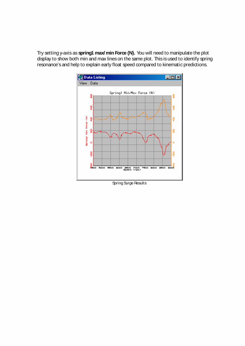
Try setting y-axis as spring1 max/min Force (N). You will need to manipulate the plot display to show both min and max lines on the same plot. This is used to identify spring resonance’s and help to explain early float speed compared to kinematic predictions.
Spring Surge Results

Getting Started Using Lotus Concept Valve Train Tutorial 13 ‘The Dynamic Spring Module’
94
Overview This tutorial introduces the concavity tool. This utility function provides an automatic method for the removal of a concave region(s) of a camshaft lobe to be replaced with a convex region. The radius of curvature at the ends of the replaced section is blended into the new convex section up to a user defined maximum positive radius. An iterative approach is used to search for the best match to the specified end conditions of gradient and radius. The iteration involves modifying the function that defines the variation of the radius of curvature between the end points and the mid point, which is in the form y=ax^n + bx + c. This tutorial includes the following sections:
n The Concavity Tool, an overview, 96
n Opening the Concavity Tool, 97
n Loading the Cam Lobe Surface Data, 98
n Analysing the Cam Lobe, 99
n The ‘General Settings’, 99
n Running the Auto Correction, 100
n Running a Manual Correction, 101
n Applying the Changes, 101
15 Tutorial 14. The Concavity Tool
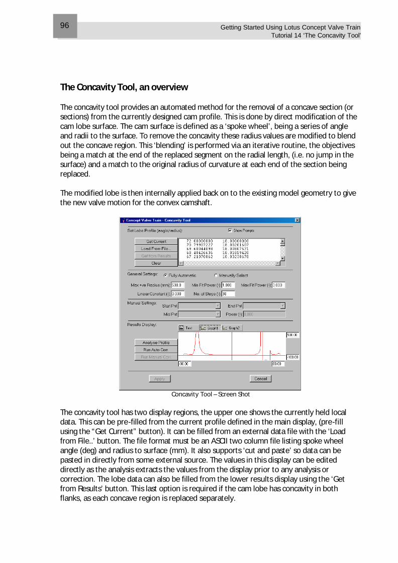
Getting Started Using Lotus Concept Valve Train Tutorial 14 ‘The Concavity Tool’
96
The Concavity Tool, an overview The concavity tool provides an automated method for the removal of a concave section (or sections) from the currently designed cam profile. This is done by direct modification of the cam lobe surface. The cam surface is defined as a ‘spoke wheel’, being a series of angle and radii to the surface. To remove the concavity these radius values are modified to blend out the concave region. This ‘blending’ is performed via an iterative routine, the objectives being a match at the end of the replaced segment on the radial length, (i.e. no jump in the surface) and a match to the original radius of curvature at each end of the section being replaced. The modified lobe is then internally applied back on to the existing model geometry to give the new valve motion for the convex camshaft.
Concavity Tool – Screen Shot
The concavity tool has two display regions, the upper one shows the currently held local data. This can be pre-filled from the current profile defined in the main display, (pre-fill using the “Get Current” button). It can be filled from an external data file with the ‘Load from File..’ button. The file format must be an ASCII two column file listing spoke wheel angle (deg) and radius to surface (mm). It also supports ‘cut and paste’ so data can be pasted in directly from some external source. The values in this display can be edited directly as the analysis extracts the values from the display prior to any analysis or correction. The lobe data can also be filled from the lower results display using the ‘Get from Results’ button. This last option is required if the cam lobe has concavity in both flanks, as each concave region is replaced separately.
Getting Started Using Lotus Concept Valve Train Tutorial 14 ‘The Concavity Tool’
97
The lower display region shows the results from either an analysis of the currently held local surface data, or the results after a concavity removal has been performed. The results’ display can be either a text listing of the angle, surface radius and radius of curvature, or a graph plot of the radius of curvature against surface angle (graph1) or a graph plot of the radius to the surface against surface angle (graph2). The iterative process employed in the concavity replacement involves changing the coefficients used to define the relationship of the variation in the cam radius of curvature from each end point to the mid-point. The iteration process also tries moving the ‘mid point’ to improve the fit and also if unable to obtain a suitable match extends the end points so that the modification is applied to a larger portion of the lobe surface. The equation used for the variation of the cam radius of curvature is;
y = ax^n +bx + c The coefficient ‘b’ is set directly, defined as the ‘linear constant’ in the interface. The power term ‘n’ is varied by the iteration process between the limits set by the ‘Min fit Power’ and ‘Max fit Power’ interface values with the number of incremental power values steps set by ‘No of Steps’ in the interface. The constants ‘a’ and ‘c’ are calculated at each increment of power to achieve a match on the radius of curvature at the boundaries of the start (or end) of the segment and the mid point. The radius of curvature at the mid-point is limited to the defined ‘Max +ve Radius’ set in the interface. As part of the iteration process the actual maximum +ve radius at the mid-point is reduced from the defined maximum to assist in matching the boundary conditions. Opening the Concavity Tool Before opening the concavity tool we will create a concave profile to use in the rest of this tutorial. Select the File / New (all) menu and in the ‘new’ dialogue display set the type to ‘Centre Rocker’, set the motion to ‘Cam Motion’ and set the curve type to ‘6 segment Polynomial, 11 points’. Select ‘Ok’ to create the new profile. If you select the ‘statics’ section plot the ‘Radius of Curvature’ to confirm that the profile is concave on the opening flank. For later comparison with our modified profile take a scope copy of the current profile and results, (menu Graph / Scope / Store / Current (Exclusive).
Getting Started Using Lotus Concept Valve Train Tutorial 14 ‘The Concavity Tool’
98
Plot of example ‘concave’ profile – prior to modification
To open the concavity tool select the menu Tools / Concavity Tool… this then displays the concavity tool dialogue box. The initial prompt indicates how to load the data and analyse the current profile. The prompts can be locally turned ‘off’ via the check box at the top of the display. Loading the Cam Surface Data To load the existing cam profile data into the local display, select the ‘Get Current’ button, this will display a text listing of the current cam lobes ‘spoke wheel’ definition. Again a prompt suggests the next step in the process would normally be to analyse the lobe details to confirm concavity.
Profile Data Loaded
Getting Started Using Lotus Concept Valve Train Tutorial 14 ‘The Concavity Tool’
99
Analysing the Cam Lobe With the cam lobe data now loaded we can analyse it to determine / check that the lobe is concave and how many concave sections its has. You don’t have to do this ‘analysis’ step you can move straight on to the ‘correcting’ phase but it does enable you to both confirm and identify the lobe concavity. Select the ‘Analyse Profile’ button. The prompt in this instance will confirm that the profile has a single concave region. Similar information prompts are shown for lobes with multiple concave regions and for convex cams. The results are loaded in to the lower display, showing either text or one of the graph options as selected.
Analysis display for original lobe
Note that the display appears to have the concave portion on the opposite side from that shown in the main display. Remember that the plot in the main display ‘statics’ section is plotted against cam rotation angle, whilst the concavity tool is plotting against cam lobe surface angle. The +ve –ve surface angle switch is due to camshaft rotation direction. The General Settings The variables given in the ‘General Settings’ area are used by the fitting routine to control the allowable boundaries for the iteration and the number of steps used between the limits. A brief description of each is given below; Max +ve Radius (mm): Defines the limit for the convex (+ve) radius that can be used by the fitting process, (fit will normally end up with an actual value that is less than this). Min Fit Power (-): Sets the minimum limit for ‘n’ the power term in the radius variation equation. The fitting routine varies ‘n’ from this value up to the maximum values using the defined number of steps in its attempt to match the required boundary conditions.
Getting Started Using Lotus Concept Valve Train Tutorial 14 ‘The Concavity Tool’
100
Max Fit Power (-): Sets the maximum limit for ‘n’ the power term in the radius variation equation. The fitting routine varies ‘n’ from the minimum value up to this maximum value using the defined number of steps in its attempt to match the required boundary conditions. No of Steps (-): Indirectly sets the step size (by defining the number of step) used by the fitting routine between the maximum and minimum values for ‘n’. Linear Constant (-): Defines a value for the ‘b’ coefficient in the radius of curvature function. It is not changed by the iterative process and it is intended for more advanced use on cases that have high +ve radius of curvature values on the end points. Running the Auto Correction We will use the default values for the ‘General Settings’ ,Max positive radius = 500 mm, Min fir power = 1.0, max fit power = 3.0, Linear constant = 0.0 and No. of steps = 30. Run the automatic correction by selecting the ‘Run Auto Corr.’ Button adjacent to the lower display. This will then take a few seconds to perform the iteration, before opening a prompt to confirm the correction is complete and then updating the results display. Note also that the values in the ‘Manual settings’ area that are greyed out when in ‘Fully Automatic’ mode are filled with the values identified by the automatic fit. This is useful for later cases where we may want to run specific manual corrections. In addition the actual maximum +ve radius of curvature value is copied back into the General Settings Area.
After auto correction – Modified settings ringed
Getting Started Using Lotus Concept Valve Train Tutorial 14 ‘The Concavity Tool’
101
Running a Manual Correction The manual correction performs a single pass with the defined data fields. The iteration within a manual correction is limited to varying the maximum +ve radius to try and match the end radius. As an example change to ‘Manually Select’, and try setting the Maximum +ve radius to 1000 mm, set the mid point to ’19 51.0018’ and set the Power to 1.5. Select the ‘Run Manual Corr.’ Button and notice the change in the displayed results.
Manual Correction results
Applying the Changes To modify the actual profile in the main display we need to apply the changes to the model. To do this select the ‘apply’ button. This takes the modified camshaft lobe and applies it back to the model. To do this the data type is switched from being defined by the polynomial to defined by individual points. This is because the polynomial definition is no longer valid and to achieve the required concavity we have to define the lobe point by point. Selecting ‘apply’ will close the concavity tool and update the display to show the new enforced cam motion. With our ‘scope’ function that we selected before opening the concavity tool we can visually compare the changes made to the valve train motion.
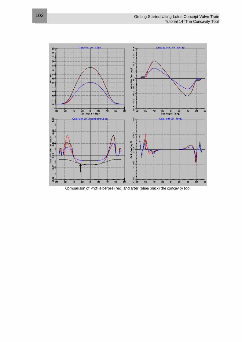
Getting Started Using Lotus Concept Valve Train Tutorial 14 ‘The Concavity Tool’
102
Comparison of Profile before (red) and after (blue/black) the concavity tool