A research report in support of the “Owner’s Guide to Maximizing Success in
Integrated Projects,” available for download from bim.psu.edu/delivery
January 2014
A report for the Charles Pankow Foundation
and Construction Industry Institute
Study authors:
Dr. Keith Molenaar
University of Colorado Boulder
Dr. John Messner
Penn State University
Dr. Robert Leicht
Penn State University
Dr. Bryan Franz
Penn State University
Dr. Behzad Esmaeili
University of Nebraska-Lincoln

ii
TABLE OF CONTENTS
LIST OF FIGURES ........................................................................................................... vi
LIST OF TABLES ............................................................................................................ vii
GLOSSARY OF TERMS ................................................................................................ viii
EXECUTIVE SUMMARY ................................................................................................ x
Chapter 1: INTRODUCTION............................................................................................ 1
Research Objectives ..................................................................................................2
Research Scope .........................................................................................................3
Research Approach ...................................................................................................4
1.3.1 Formation of the Industry Advisory Board ..................................................4
1.3.2 Develop the Survey Questionnaire ...............................................................6
1.3.3 Collect Completed Project Data ...................................................................6
1.3.4 Verify Survey Response Data .......................................................................7
1.3.5 Perform Multivariate Data Analysis .............................................................7
1.3.6 Develop Owners Guide to Apply Findings ..................................................7
Research Results .......................................................................................................8
Benefits to the Industry ............................................................................................8
Reader’s Guide ..........................................................................................................9
Chapter 2: LITERATURE REVIEW............................................................................... 10
Project Delivery Methods .......................................................................................10
Procuring a Team for Success .................................................................................14
Payment Terms .......................................................................................................15
Organizational Collaboration ..................................................................................16
Stages of Group Development ................................................................................17
Strategies to Reduce Fragmentation .......................................................................18
The Project Organization and Integration ...............................................................20
Chapter Summary ...................................................................................................20

iii
Chapter 3: THEORETICAL FRAMEWORK ................................................................. 21
A Framework for Studying Team Integration .........................................................21
Project Delivery Strategy ........................................................................................23
3.2.1 Delivery Method .........................................................................................23
3.2.2 Procurement Process ...................................................................................25
3.2.3 Contractual Terms .......................................................................................26
Team Integration .....................................................................................................27
Group Cohesiveness ................................................................................................30
Project Performance ................................................................................................32
3.5.1 Cost Metrics ................................................................................................32
3.5.2 Schedule Metrics .........................................................................................34
3.5.3 Quality Metrics ............................................................................................35
3.6 Programming Factors ..........................................................................................36
3.6.1 Owner Type .................................................................................................36
3.6.2 Facility Size .................................................................................................36
3.6.3 Facility Type ...............................................................................................37
Data Collection Tool ...........................................................................................38
3.7.1 Pilot Testing ................................................................................................39
3.7.2 Section 1: Project Characteristics ................................................................40
3.7.3 Section 2: Project Organization ...................................................................40
3.7.4 Section 3: Project Cost ................................................................................40
3.7.5 Section 4: Project Schedule .........................................................................41
3.7.6 Section 5: Project Quality ...........................................................................41
3.7.7 Section 6: Project Safety .............................................................................41
3.7.8 Section 7: Sustainability ..............................................................................41
3.7.9 Section 8: Team Procurement and Contracts ..............................................42
3.7.10 Section 9: Team Characteristics and Behavior .........................................42
3.7.11 Section 10: Process and Technology .........................................................42
3.7.12 Section 11: Lessons Learned .....................................................................43
Chapter Summary ...................................................................................................43
Chapter 4: DATA COLLECTION AND ANALYSIS METHODS ................................ 44
Data Collection Methods ........................................................................................44
4.1.1 Survey Distribution .....................................................................................45

iv
4.1.2 Data Recording and Verification .................................................................46
4.1.3 Data Screening ............................................................................................47
Data Analysis Methods ...........................................................................................49
4.2.1 Latent Class Formation ...............................................................................50
4.2.2 Structural Equation Modeling .....................................................................50
Sources of Bias ........................................................................................................52
4.3.1 Self-Selection Bias ......................................................................................52
4.3.2 Non-Response Bias .....................................................................................52
Chapter Summary ...................................................................................................53
Chapter 5: LATENT CLASS MODEL OF DELIVERY ................................................ 54
Preparing for Latent Class Analysis ........................................................................54
5.1.1 Coding of Indicator Variables .....................................................................55
5.1.2 Identifying Poor Differentiators ..................................................................58
Comparing LCA Models .........................................................................................58
Selecting the Best-Fit LCA Model ..........................................................................60
A Five-Class Model of Project Delivery Strategies ................................................62
5.4.1 Class Assignment using Posterior Probabilities ..........................................64
5.4.2 Detailed Description of Classes ..................................................................65
Chapter Summary ...................................................................................................71
Chapter 6: STRUCTURAL MODELING RESULTS ..................................................... 72
Data Demographics .................................................................................................72
Construct Validity of Latent Factors .......................................................................77
6.2.1 Measurement Variable Correlations ............................................................78
6.2.2 Initial Confirmatory Factor Analysis ..........................................................79
6.2.3 Exploratory Factor Analysis ........................................................................80
6.2.4 Poorly Fitting Measurement Variables .......................................................81
6.2.5 Revised Confirmatory Factor Analysis .......................................................82
Factoring Performance Outcomes ...........................................................................83
Specifying the Structural Model .............................................................................85
Primary Structural Model Results ...........................................................................88
6.5.1 Cost Performance ........................................................................................92
6.5.2 Schedule Performance .................................................................................93
6.5.3 Quality Performance ...................................................................................95
v
6.5.4 Summary of Primary Results ......................................................................96
Secondary Structural Model Results .......................................................................98
6.6.1 Team Integration .........................................................................................98
6.6.2 Group Cohesiveness ....................................................................................98
6.6.3 Summary of Secondary Results ..................................................................99
Chapter Summary .................................................................................................100
Chapter 7: SUMMARY AND CONCLUSIONS .......................................................... 101
Summary of Findings ............................................................................................101
Research Contributions .........................................................................................106
Industry Applications ............................................................................................109
7.3.1 Review of Existing Project Delivery Selection Tools ...............................109
7.3.2 Owner’s Guide Format ..............................................................................110
Limitations ............................................................................................................112
Future Research .....................................................................................................114
Concluding Remarks .............................................................................................115
REFERENCES ............................................................................................................... 117
Appendix A: DATA COLLECTION TOOL ................................................................. 127
Appendix B: LATENT CLASS DESCRIPTIONS ........................................................ 131
Appendix C: DESCRIPTIVE STATISTICS ................................................................. 132
Appendix D: EXPANDED STRUCTURAL MODEL .................................................. 136
Appendix E: WHITE PAPER ........................................................................................ 137
Appendix F: OWNER’S GUIDE ................................................................................... 151
Appendix G: DISSEMINATION PLAN ....................................................................... 153

vi
LIST OF FIGURES
Figure 2-1: Collaboration continuum interpretations in literature .................................... 16
Figure 3-1: Theoretical model of research variables ........................................................ 22
Figure 5-1: Probabilities of having each indicator variable for the five latent classes ..... 63
Figure 5-2: Involvement for contractors based on posterior class assignments ............... 66
Figure 5-3: Procurement process for contractors based on posterior class assignments .. 68
Figure 5-4: Selection criteria for contractors based on posterior class assignments ........ 69
Figure 5-5: Payment terms for contractors based on posterior class assignments ............ 70
Figure 6-1: Distribution of projects by facility type ......................................................... 73
Figure 6-2: Distribution of facility type by class of project delivery strategy .................. 74
Figure 6-3: Distribution of project size by square footage ............................................... 75
Figure 6-4: Distribution of sample projects across the United States ............................... 76
Figure 6-5: Distribution of project unit cost in dollars per square foot ............................ 77
Figure 6-6: Revised CFA with unstandardized (A) and standardized (B) estimates ........ 83
Figure 6-7: Specification of structural model alternatives ................................................ 86
Figure 6-8: Unstandardized estimates for structural model paths .................................... 90
Figure 6-9: Structural model diagram and results with standardized estimates ............... 91

vii
LIST OF TABLES
Table 2-1: Summary of studies examining delivery method and performance ................ 11
Table 3-1: Semantic differential adjectives used to evaluate group cohesiveness ........... 30
Table 3-2: Facility type classifications ............................................................................. 38
Table 4-1: Summary of data collection methodology....................................................... 45
Table 4-2: Actions for resolving multiple response discrepancies ................................... 48
Table 4-3: Summary of data analysis methodology ......................................................... 49
Table 5-1: Dichotomous classifications of delivery strategy indicators ........................... 56
Table 5-2: Item-response frequencies for delivery strategy indicators ............................. 57
Table 5-3: Fit indices, selection criterion and ratio test for latent class solutions ............ 60
Table 5-4: Item-response probabilities for the four-class solution ................................... 61
Table 5-5: Item-response probabilities for the five-class solution .................................... 62
Table 6-1: Correlation coefficients for team measures ..................................................... 79
Table 6-2: Rotated loadings for 2-factor EFA of team measures ..................................... 81
Table 6-3: Correlation coefficients for project performance variables ............................. 84
Table 6-4: Rotated loadings for 2-factor EFA of quality ratings ...................................... 85
Table 6-5: Fit indices of structural model alternatives ..................................................... 87
Table 6-6: Predictive capability of structural model alternatives ..................................... 88
Table 6-7: Summary of primary outcome relationships from structural model ............... 97
Table 6-8: Summary of secondary outcome relationships from structural model .......... 100
Table 7-1: Summary of project delivery selection efforts in literature ........................... 110
Table B-1: Summary of project delivery classes……………………………………….131
Table C-1: Descriptive statistics for group cohesiveness measures……………………132
Table C-2: Descriptive statistics for team integration measures……………………….133
Table C-3: Descriptive statistics for cost and schedule metrics………………………..134
Table C-4: Descriptive statistics for quality measures…………………………………135

viii
GLOSSARY OF TERMS
Group cohesiveness: The degree to which project team members function as a single
unit. In organizational research, the development of cohesion is believed to mark the
transition from a coordinated work group to a collaborative team. Represented in this
study as a latent variable, group cohesiveness is measured by goal commitment, team
chemistry and timeliness of communication.
Project delivery strategy: A categorization system that represents common
combinations for the owner’s project delivery decisions, as seen in practice. In this
study, each delivery strategy corresponds to a set of indicators derived from key
differentiators of delivery methods, procurement processes and contractual terms. These
indicators include the use of a single contract for design and construction, timing of
involvement of builder and trades, use of a prequalification step in procurement, a cost-
of-work based selection and the award of an open book contract to the builder.
Project organization: The temporary contractual arrangement of design and
construction disciplines, structured by the owner, with the mission of delivering an
operational building. In the project organization, participants remain a member of their
parent organization, but have the added responsibility of becoming a contributing
member of the project team. In this study, the project delivery strategy is considered as a
driver of the structure and boundaries of the project organization.
Project team: The primary participants in a building construction project and the group
tasked with the management and execution of project organization’s mission. The
consistent project team captured in this study is represented by the owner, architect,
primary contractor or construction manager, mechanical and electrical trade contractors
and structural trade contractors.

ix
Team integration: The degree to which project team members from separate parent
organizations engage in collaborative practices. A highly integrated team will leverage
the expertise of individual members to improve the project delivery process. Represented
in this study as a latent variable, team integration is measured by participation in joint
goal-setting, design charrettes, greater use of Building Information Modeling (BIM) and
co-location during construction.
x
EXECUTIVE SUMMARY
The architecture, engineering and construction (AEC) industry is often criticized for
its fragmented approach to project delivery. Traditional procurement and contracting
structures serve to isolate designers from contractors, limiting opportunities for
collaboration. Viewed as the logical solution to fragmentation, team integration is the
process of bring design and construction disciplines back together. Team integration has
recently attracted the attention of building owners, made weary by the adversarial
relationships common in traditional delivery. However, there is limited empirical
evidence linking more integrated teams with improved project performance.
This research presents a structural modeling approach to studying the role of team
integration in construction project performance. The focus of this research is the project
organization, a temporary team of design and construction disciplines that forms for the
duration of the project. Project organizations often consist of team members who have
never worked together before and will disperse at the completion of the contracted scope.
Recognizing the importance of team development in organizations, this research also
considers the role of group cohesiveness in delivering a successful project. A sample
data set of 204 building projects was used to compare cost, schedule and quality
performance under different project organizations. To characterize the types of project
organizations seen in industry, a latent class analysis was performed to group projects by
their delivery strategy. Path analysis revealed complex relationships between the
delivery strategy, team integration, group cohesiveness and project performance.
Integrated teams involved all tiers of the project organization, from designers to
specialty contractor trades, in high-quality interactions. These interactions were
collaborative in nature and included design charrettes, goal setting and multidisciplinary
BIM uses. The owner’s project delivery strategy had a significant impact on team
integration. Strategies that involved construction managers and specialty contractor

xi
trades before schematic design achieved higher levels of integration and were more
equipped to control project schedule growth. Cohesive teams reported higher chemistry,
goal commitment and timeliness of communication. Project delivery strategies that
required cost transparency with open book contracts generally resulted in a more
cohesive teams and a lower average project cost growth. Additionally, the owner’s
perception of turnover experience and building system quality was consistently rated
higher for cohesive teams.
Understanding these relationships will make building owners more aware of how
early project delivery decisions influence the development of their project teams. Based
on their specific goals, owners may select a project delivery strategy that creates the
appropriate team environment for the project. The findings of this research are poised to
expand methods for studying and implementing project organizations.

1
Chapter 1
INTRODUCTION
Due to a lack of experience and objective performance data, owners often make
project delivery decisions on the basis of personal preference or comfort level.
Organizational acquisition policies also constrain owners’ decisions and are difficult to
change without evidence-based comparisons of alternative project delivery approaches.
There is a growing need among owners in the architecture, engineering and construction
(AEC) industry for objective data on the performance impacts of their early project
delivery decisions.
In 1997, the Construction Industry Institute (CII), led by the research of Victor
Sanvido and Mark Konchar of Pennsylvania State University (Penn State) and CII
Research Team 133, conducted seminal research in project delivery performance. The
project entitled “Project Delivery Systems: CM at Risk, Design-Build, Design-Bid-
Build,” examined project performance based on data from more than 350 projects and
provided owners with guidance on delivering successful projects (CII 1997). The
resulting research report provided data to support the owner’s project delivery decision-
making and contributed fundamental knowledge on the integration of design and
construction disciplines. This information was pivotal in helping the industry shift away
from the traditional design-bid-build method of project delivery to more integrated
arrangements, including design-build and construction management at risk (Konchar and
Sanvido 1998, Molenaar, et al. 1999, El Wardani et al. 2006).
Since the publication of the original Penn State/CII study in 1997, the industry has
evolved substantially, particularly in the area of team integration. The crisp lines that
previously defined the three delivery methods of design-bid-build, design-build, and
construction manager at risk have become blurred. Integrated project delivery

2
arrangements have arisen with the drafting of multi-party contracts (AIA C191-2009;
ConsensusDOCS 300), but few projects with true multi-party contracts have been
completed due to owner’s operational, legal and cultural constraints. Owners are
attempting to implement pieces of the integrated project delivery process in hopes of
improving project success (El Asmar and Hanna 2013). Owner’s now need empirical
evidence to assist them in selecting an overall project delivery strategy that addresses
team organization, procurement processes, and contract payment methods. This strategy
results in a project environment that is more conducive to developing team integration
and group cohesion in support of improving project outcomes.
Team integration is seen as the logical solution to fragmentation in the construction
industry. Baiden and Price (2011) define team integration as “where different disciplines
or organizations with different needs and cultures merge into a single cohesive and
mutually supporting unit.” Integration has been suggested to improve project
performance (Egan 2002; Payne et al. 2003), but the empirical evidence linking the two
concepts is limited. Quantifiable examples of successfully integrated teams are scarce,
although at least one exception demonstrates the benefits of integration using case studies
from practice (Constructing Excellence 2004).
Group cohesion has historically been considered the most important variable in
studying small groups (Carron and Brawley 2000). More cohesive groups perform better
in organizations where efficiency is an important goal, as opposed to simply the
successful completion of the task (Beal et al. 2003). The concept of group cohesion has
applications to project teams in the construction industry, who are tasked with delivering
a facility within the owner’s time and budget constraints, while maintaining the desire
level of quality and functionality of the facility.
Research Objectives
The research seeks to determine, analytically and without bias, the role of project
delivery methods and the project team in project success. The research explores

3
successful owner practices regarding roles, team integration, team behavior, delivery
methods, procurement methods, and project performance in the building design and
construction industry. The research ultimately uses the constructs of team integration and
group cohesiveness to better understand how the elements of a project delivery strategy
relate to cost, schedule and quality performance. Specifically, the research project
addressed the following essential and supporting research questions:
1. How can the owner contribute to the successful delivery of their project?
a. What, from an owner’s point of view, is the project delivery success?
b. What approaches must an owner undertake to promote a successful project
environment?
2. How do the project delivery method, procurement process and contractual
payment terms impact project success?
3. How does project team integration impact project delivery success?
a. What attributes can be used to identify the level of team integration, and
how are those tied to the industry definitions of project delivery systems?
4. How does team behavior (i.e., group cohesion) impact project success?
a. What attributes can be used to identify the cohesiveness of the team, and
how are those tied to the industry definitions of project delivery systems?
Research Scope
This study collected project information for a subset of projects in the general
building industry. These projects were predominantly new construction and located only
within the United States. They were completed between 2008 and 2013. This sample
specifically excludes renovations, civil or highway work, single-family residential,
international projects and older or incomplete projects. Performance measurements were
limited to cost, schedule and quality metrics. Construction and total project costs were
documented at the time of contract award and at final completion. Schedule dates were
requested for design start, construction start and substantial completion. Quality was
assessed on a semantic differential scale (i.e. Likert scale) that asked owners to rate their

4
turnover experience and overall system quality in the facility. Lastly, various measures
of group cohesiveness and indicators of integrated processes were captured to assist with
defining team behaviors and relationships.
Research Approach
This research was divided into six phases. First, an industry Advisory Board was
formed to assist in scoping the research and creating the data collection questionnaire.
Next, a survey questionnaire was developed to collect detailed information on recently
completed buildings from project participants. This survey was created with a
combination of literature review and feedback from the Advisory Board. The survey
captured quantitative cost, schedule and quality data, as well as qualitative perceptions of
the team behaviors and group cohesiveness. Phase three broadly distributed the survey
across the United States using mailing lists for various AEC professional organizations.
Phase four focused on the verifying the quality of the submitted data and the research
team spent extensive time following-up with survey respondents on key project
information. The fifth phase applied multivariate analysis techniques to simultaneously
model project delivery strategy, team integration and group cohesiveness with project
performance outcomes. The final phase leveraged the results to develop an owner’s
guide for project delivery that provides a structured approach to apply the findings in the
AEC industry. This final phase also employed the Advisory Board for validation of the
results and appropriate interpretation for the guide development. Each of these phases is
discussed in greater detail in the sections that follow.
1.3.1 Formation of the Industry Advisory Board
The research team worked with two industry champions, Mr. Greg Gidez, Corporate
Director for Preconstruction and Design Management Services for Hensel Phelps
Construction Co., and Dr. Mark Konchar, Vice President Business Acquisition for
Balfour Beatty Construction, to form an industry Advisory Board with leaders from the
design and construction industry. These leaders were chosen through their active

5
participation with the Charles Pankow Foundation, the Construction Industry Institute
and through the recommendations of other panel participants. The Advisory Board
assisted the team with the development of the final data collection questionnaire, helped
with testing, contributed project data to the study, and reviewed the final results. The
following members actively participated in the project:
Mr. Greg Gidez (co-chair), Hensel Phelps Construction Co.
Dr. Mark Konchar (co-chair), Balfour Beatty Construction
Mr. Howard W. Ashcraft, Esq., Hanson Bridgett LLP
Dr. Russell Manning, Department of Defense
Mr. Spencer Brott, Trammell Crow Real Estate Services, Inc.
Dr. John Miller, Barchan Foundation, Inc.
Mr. Bill Dean, M.C. Dean, Inc.
Mr. Brendan Robinson, U.S. Architect of the Capitol
Mr. Tom Dyze, Walbridge
Dr. Victor Sanvido, Southland Industries
Mr. Matthew Ellis, US Army Corps of Engineers
Mr. Ronald Smith, Kaiser Permanente
Ms. Diana Hoag, Xcelsi Group, LLC
Mr. David P. Thorman, FAIA, Former California State Architect
Mr. Mike Kenig, Holder Construction
The Advisory Board met in person four times over the course of the research project
and periodically through telephone or internet conferences. To ensure that all industry
members had a common vocabulary and understanding in regards to research in project
delivery, the research team developed a white paper for distribution before the first
Advisory Board meeting. The white paper, entitled “Owner’s Guide to Maximizing
Success in Integrated Projects: A Summary of Study Performance Metrics,” is included
in Appendix E of this report.

6
1.3.2 Develop the Survey Questionnaire
The survey questionnaire underwent both internal and external pilot testing prior to
distribution. The internal pilot included four projects for which the project owner was
contacted via phone and completed a survey-style interview on a paper-based version of
the survey. The external pilot was a test of both the survey distribution methodology and
an electronic, web-based version of the survey. A letter of introduction to the study and a
link to the survey were distributed via email to a small sampling of industry contacts. The
external pilot produced twelve responses for ten unique projects. The result of the pilot
process was eliminating several redundant and onerous questions to shorten the length of
the survey. A final version of the survey questionnaire is provided in Appendix A. The
survey was separated into eleven sections to collect information on the delivery of the
project, organizational integration, team behaviors and performance outcomes.
Additional information on the survey and specific sections can be found in Chapter 3.
1.3.3 Collect Completed Project Data
Data were collected by email and postal mail distribution of the survey questionnaire.
Portable Document Format (PDF) form versions of the questionnaire were emailed to the
national mailing lists for multiple design and construction professional organizations.
These included the American Public Works Association (APWA), Association of Higher
Education Facilities Officers (APPA), the Construction Management Association of
American (CMAA), the Construction Owners Association of America (COAA), the
Design-Build Institute of America (DBIA), the Federal Facilities Council (FFC), the
Higher Education Facilities Management Association (HEFMA) and the Partnership for
Achieving Construction Excellence (PACE) at Penn State. These organizations were
selected because they have diverse memberships across the building industry. Paper
versions of the survey were mailed to alumni from Penn State’s Architectural
Engineering program and PDF versions were sent to the alumni from the University of
Colorado’s Department of Civil, Environmental and Architectural Engineering and the
Real Estate Development program. These alumni groups were selected to increase the
rate of response on the survey due to the individual’s previous affiliation with the

7
industry. To avoid bias, all respondents were asked to complete the survey for their most
recently completed building project. No specific type of facility was targeted in this
research. Projects in the data set represented the general building sector, which includes
both simple and complex facilities.
1.3.4 Verify Survey Response Data
A member of the research team at Penn State or the University of Colorado Boulder
verified each survey response. The verification procedure included an email and/or
phone call to the respondent to confirm key project information and obtain any missing
data. If a contractor or designer returned the survey, efforts were made to contact the
project owner directly. Completed responses were entered into a Microsoft Access®
database using form inputs to reduce the likelihood of data entry errors. After completing
the data collection phase, verified data was exported to a Microsoft Excel spreadsheet for
screening. Unverified projects and those outside the scope of the research were removed
from the data set, leaving a total of 204 projects for analysis. Descriptive statistics of the
data were reviewed for out-of-range values and outliers.
1.3.5 Perform Multivariate Data Analysis
Using MPlus statistical software, a latent class analysis was performed to classify
each project by their most likely project delivery strategy. These classifications were
based on response patterns to survey questions on the delivery method, procurement
processes and contractual terms. Next, a confirmatory factor analysis was run to validate
the constructs of team integration and group cohesiveness. Lastly, relationships between
the class of project delivery strategy, team integration, group cohesiveness and project
performance were investigated using structural equation modeling.
1.3.6 Develop Owners Guide to Apply Findings
To apply the findings, the research team developed a structured owner’s guide for
making early project delivery decisions. The research team investigated multiple guides
8
that had been published in the literature and/or applied in practice before ultimately
choosing a five-step process for selecting the appropriate project delivery strategy. This
structured approach requires the owners to: (1) define project goals and constraints; (2)
consider team organization options; (3) consider contract payment methods; (4) consider
team procurement processes; and (5) select a project delivery strategy. All five of these
steps seek to increase the aspects of team integration and group cohesion that were found
to influence success. Ultimately, each project is unique and there is no one project
delivery strategy that is appropriate for every project. However, this owner’s guide will
help to promote team integration and group cohesion, two constructs that were found to
influence success, in all project delivery strategies.
Research Results
The primary results of this research include:
1. A classification of project delivery strategies, using differentiators of team
organization, procurement processes and contractual terms;
2. The use of latent constructs to represent team integration and group cohesiveness
in construction projects;
3. The use of structural equation modeling to begin exploring the mechanisms by
which project teams yield more desirable project outcomes; and
4. An owner’s project delivery selection guide with a structured process by which
owners can apply the results of this research to increase the likelihood of
achieving team integration, group cohesiveness, and ultimately overall project
success.
Benefits to the Industry
The primary benefit to the construction industry is to provide a repeatable process for
making highly effective, early project delivery decisions. It will allow owners to select
delivery methods, project teams and contracting methods that offer the greatest likelihood
9
of success. A second benefit to public sector owners will be to help them demonstrate a
transparent decision-making process regarding delivery method, as well as assurance of
cost and schedule savings, attainment of best value for the dollar, and quality outcomes.
Underlying both of these benefits is an enhanced understanding of how team integration
and group cohesion affect project success in the AEC industry. The basic knowledge is
being disseminated through academic research journals and the applied knowledge is
being disseminated at industry conferences and through the application of the user’s
guide.
Reader’s Guide
Chapter 1 provided an introduction to the research including: a review of relevant
literature to contextualize the problem statement and an overview of the research
approach. Chapter 2 presents a literature review that identifies the gap in knowledge that
serves as the motivation of this research. Chapter 3 describes the theoretical framework
for this research, defines the variables used in the analysis and provides an overview of
the survey questionnaire. The data collection and analysis methods are discussed in
Chapter 4. Chapter 5 presents the latent class analysis and descriptions of the resulting
classes of project delivery strategy used in this research. Chapter 6 explains the sample
data set and describes the detailed results of the structural equation modeling effort.
Lastly, Chapter 7 summarizes the findings of this research, presents the background for
the development of the owner’s project delivery selection guide, acknowledges
limitations in the methodology, discusses contributions and provides an outline for future
research.

10
Chapter 2
LITERATURE REVIEW
This chapter reviews current literature on empirical studies that relate project delivery
and project performance, with specific emphasis on the owner’s role in the delivery
process. The gap in literature related to the role of team integration in construction
project performance is identified. Background on the AEC industry leading up the
present state of fragmented teams is reviewed and discussed with attention also given to
organizational studies on team integration. Additional literature on project delivery
methods, procurement processes and contractual terms are reviewed in Chapter 3
alongside the development of a theoretical model for this research.
Project Delivery Methods
Key owner decisions made during the early stages of a project, such as selecting a
delivery method, team members or a contractual payment method, have a role in
determining project success (Konchar and Sanvido 1998). There is a growing interest
among owners to understand the relationships between key decisions and their impact on
typical definitions of project success, such as cost growth, schedule growth and quality.
In response, a number of studies have compared the performance of common forms of
project delivery (e.g. Konchar and Sanvido 1998; Ibbs et al. 2003; Hale et al. 2009; El
Asmar et al. 2013). The objective of these studies was to help owners to understand the
implications of their decisions with more objectivity by providing empirical data.
Historically, project delivery methods have been found to influence project outcomes
in large-scale statistical studies. Several of these studies were conducted to compare the
performance of construction projects under design-bid-build, design-build, and

11
construction management at risk delivery methods (Pocock et al. 1996; CII 1998;
Konchar and Sanvido 1998; Molenaar et al. 1999; and Gransberg et al. 1999). A
summary of significant empirical studies related to delivery systems are presented at
Table 2-1. No study concluded a significant relationship between specific delivery
method and better quality performance.
Table 2-1: Summary of studies examining delivery method and performance
Study Type of
Project
Sample
Size Significant Findings
Konchar and Sanvido (1998) General 351
Unit cost: DB < CMR < DBB
Cost growth: DB < DBB < CMR
Schedule growth: DB < CMR < DBB
Delivery speed: DBB < CMR < DB
Construction speed: DBB < CMR < DB
Ibbs et al. (2003) -- 67 Schedule Growth: DB < DBB
Hale et al. (2009) Military 77 Cost Growth: DB < DBB
El Asmar et al. (2013) Institutional 35
The following metrics were
significantly different for IPD and non-
IPD projects (p-value=.01):
Change order processing time
Deficiency issues
Request for information
Punch list costs
Notes: DBB=Design-bid-build; CMR=Construction manager at risk; DB=Design-build
The Construction Industry Institute (CII) and Penn State University completed a
seminal study for improving project delivery method selection and as a result provided
practical decision guidelines, backed by empirical evidence (CII 1998, Konchar and
Sanvido 1998). The study included performance metrics for cost, schedule, and quality
for projects delivered under the three most common project delivery methods for
buildings in the United States. Comparing 351 building projects, the study concluded
that design-bid-build projects had statistically significant higher unit cost, and slower
construction and delivery speeds. Additionally, the design-build projects had the lowest
schedule and cost growth. While the unit cost, construction speed, and delivery speed had
12
higher levels of certainty, the variation in cost and schedule growth were not able to be
explained fully. The most prominent contribution of the study was to provide guidance
for owners on how to leverage delivery decisions to support a successful project.
In another study, Ibbs et al. (2003) analyzed characteristics of 67 global projects,
finding that design-build does not outperform design-bid-build across all project
performance criteria. The results indicated that design-build had a definite advantage on
time savings, but correlations with cost and productivity were unsupported. The study
stated that the project management expertise and experience of the contactor may have a
greater impact on project performance outcomes than delivery method alone. Hale et al.
(2009) compared the performance of 39 design-bid-build projects and 38 design-build
projects and found that design-build projects takes less time to complete and have less
time and cost growth. The strength of their study was in sampling only similar military
buildings of the same typology, which results in a more meaningful comparison (Hale et
al. 2009). Hale’s study concluded that owners selecting a design-build method can
expect less cost and schedule growth in comparison to other delivery arrangements.
In addition to design-bid-build, design-build and construction manager at risk,
researchers have examined emerging delivery systems, such as integrated project delivery
(IPD). Owners who use integrated project delivery aim to enhance project outcomes
through increasing collaboration among different party members (AIA California Council
2007). The main principals of integrated project delivery can be summarized as
multiparty agreement, early involvement of all parties, and shared risk and rewards (Kent
and Becerik-Gerber 2010). In a recent empirical study, El Asmar et al. (2013) collected
performance data of 35 completed projects and found that IPD and projects delivered
employing some elements of IPD without the multiparty contract, provided higher quality
facilities, faster and at no significant extra cost. While several studies have suggested
IPD’s superior performance to traditional delivery methods, the adoption of integrated
project delivery in the US is still very low and the evidence has been based primarily
upon case studies. The work of El Asmar et al. (2013) is suggestive of the value of a
more empirical study, but with a small pool of projects that limited the ability to delve

13
into the aspects of the integrated approach that were influential in the improved project
outcomes.
While many studies compared project performance of delivery methods for building
construction, there were also several studies conducted for highway projects. To expand
delivery method research into the civil domain, Shrestha et al. (2012) investigated the
relationship between cost and schedule metrics and the project characteristics of 130
large (>$50 million) highway projects in Texas. This study concluded that the
construction speed and project delivery speed per lane mile of design-build projects were
significantly faster than of design-bid-build projects. In another study, Minchin et al.
(2013) compared the performance of design-build and design-bid-build highway and
bridge projects at the state of Florida. In contrast with most of the previous studies, they
found that design-bid-build projects performed significantly better than design-build
projects in cost performance.
Most of the previous studies compared project performance of design-build and
design-bid-build project delivery methods for building or industrial projects; however,
there were limited studies to compare performance of these project delivery methods for
highway projects. To expand delivery method research into the civil domain, Shrestha et
al. (2012) investigated the relationship between project performance metrics (i.e., cost,
schedule, and change orders) and project characteristics of 130 large highway projects
(>$50 million) in Texas. The study concluded that the construction speed and project
delivery speed per lane mile of design-build projects were significantly faster than of
design-bid-build projects. In another study, Minchin et al. (2013) compared cost and time
performance of design-build and design-bid-build highway and bridge projects at the
state of Florida. In contrast with most of the previous studies, they found that design-bid-
build projects performed significantly better than design-build projects in terms of cost
performance.
While the contributions of these previous studies to the understanding of delivery
methods and project performance were valuable, there are several limitations. First, the
14
previously well-defined boundaries between delivery methods are becoming blurred, as
owners pursue hybrid or custom delivery arrangements. Therefore, there is a need to
explore the performance of delivery approaches based on more fundamental attributes,
such as time of involvement of different parties. Secondly, as more integrated delivery
methods are introduced, there is a need to collect empirical data and compare
performance of these new delivery systems with traditional methods. Lastly, the
performance criteria used in previous studies were limited to cost, schedule, or quality.
However, new performance criteria have been introduced in the context of delivery
decisions over the past decade, such as sustainability, safety, and owners’ satisfaction
(Wuellner 1990; Pocock et al. 1996; and Atkinson 1999). Including these success criteria
in large project delivery database can provide a better assessment of project success.
Procuring a Team for Success
Another important decision that an owner must make for a project is the approach
used to solicit and select the design and construction team. Factors within the owner’s
organization often guide the procurment decision. This is particularly true in the public
sector where agencies typically have stringent procurement rules, but it also applies to
private companies who may have policies and norms that inhibit them from trying
alternative procurement approaches.
In one study that evaluated the impact of procurement on project performance,
Molenaar et al. (1999) compared public design-build projects under three different
procurement methods: one-step, two-step, and qualifications-based. The two-step method
was found to have the least cost growth (3%) and schedule growth (2%). The one-step
projects were delivered, on average, 4% over budget and 3.5% behind the schedule.
Qualifications-based procurement had the highest cost growth (5.6%) and schedule
growth (3.5%). In another study, data from 76 design-build projects was collected to
develop a series of guidelines to help owners in selecting the design-build team aligned
with their project goals (El Wardani et al. 2006). The performance metrics were based on
the traditional outcomes of time, cost, and quality and the team selection methods were
15
sole source, qualification-based, best value, and low bid selection. While the findings of
the study illustrated that there were no specific team procurment methods that outperform
all others across every performance metric, the qualification-based selection method
showed the lowest cost growth.
Alongside typical metrics such as cost, schedule, quality and owner satisfaction, some
researchers studied the impact of project procurement methods on an owner’s
administrative burden (Molenaar and Songer 1998; Gransberg et al. 1999). According to
these studies, a qualifications-based approach is usually pursued on projects with a low
level of design completion. Using best value selection in delivery methods such as
design-build has been shown to simplify control on the project scope, cost, and time
schedule for the contractor and reduces the administrative burden on the owner’s side
(Gransberg et al. 1999).
Payment Terms
Contract payment provisions can impact the relationship between an owner and a
contractor. Three common types of payment terms are seen in practice: lump-sum, cost-
plus fee, and cost-plus a fee with a guaranteed maximum price (GMP). Characteristics of
each of these contract structures, including the time at which the price of the project is
fixed, will influence the responsibilities and roles of the contract parties (Beard et al.
2001). Bogus et al. (2010) addressed this variation by collecting project data for 99 water
and wastewater infrastructure projects completed after 2003. They study compared the
performance of projects procured under cost-plus fee with and without a guaranteed
maximum price and those with traditional lump sum payment provisions. The results
showed that the mean cost growth of projects procured under cost-plus fee with GMP
contract was significantly less than projects procured under lump sum contracts. The
direct relationship between payment terms and project performance has not been studied
extensively in the building construction industry.

16
Organizational Collaboration
Collaborative working practices are frequently discussed in literature and considered
to have a positive impact on the delivery of construction projects. Aggregating from
multiple sources, Greenwood and Wu (2012) define collaboration between parties as
“working together for mutual advantage, through which they can achieve greater benefits
than by working separately.” Although broad, this description of collaboration is closely
related to discussions on cooperation in partnerships (Bresnen and Marshall 2002) and
project team integration (Baiden et al. 2006). In organizational literature, these related
levels of ‘working together’ are often viewed as a scale or continuum as shown in Figure
2-1. Peterson (1991) suggested three stages of inter-agency interaction in care providers,
beginning with cooperation, moving to coordination and ending with collaboration.
Konrad (1996) expanded by proposing five levels for human services firms, including
information sharing, a combination of cooperation and coordination, collaboration,
consolidation and integration. Lastly, Bailey and Konley (2000) posit a similar five
levels of cooperation, coordination, coalition, collaboration and integration.
Figure 2-1: Collaboration continuum interpretations in literature
Empirical research in the AEC industry along these continuums is limited, although
two recent studies look specifically at the role of cooperation and collaboration in project
performance. Studying the Hong Kong construction industry, Phua and Rowlinson
(2004) found that cooperation and contractual characteristics were predictors of project
ConsolidationCoalitionInformation
SharingCooperation Coordination Collaboration Integration
Peterson (1991)
1 2 3
Bailey and Koney (2000)
1 2 3 4 5
Konrad (1996)
1 2 3 4 5
Informal Formal

17
success, and with varying levels of importance between contractor and consultant
organizations. An important contribution of this study was starting to identify indicators
of cooperation on projects to allow for more detailed analyses. Greenwood and Wu
(2012) attempted a similar line of inquiry, but considered the group cohesiveness by
collecting data on both positive and negative attributes of collaborative working. Their
analysis demonstrated a clear association between collaboration and the control of cost
and schedule, and the quality of work and user satisfaction on building projects.
However, these studies either ignore the concept of team integration or use delivery
methods to approximate some level of organizational integration.
Stages of Group Development
In organizational literature, a clear distinction is made between groups and teams.
Katzenbach and Smith (1993) describe a group as a collection of individuals working in
the same area or placed together to complete a task. All teams are groups, but not all
groups become teams. The transition to a team occurs when the group is committed to a
common purpose, sets performance goals and holds themselves mutually accountable for
success. Teams are not always more desirable than groups, but are more suited to higher
level tasks, such as problem-solving (Majchrzak and Wang 1996).
Studies on the stages of group development provide insight into the conditions needed
for an effective team (Tuckman 1965). The first stage, orientation to the task, occurs
when group members learn about each other and the task for which the group was
formed. Intragroup conflict is the second phase and is characterized by uneven
interactions and resistance to the task, as group members struggle to balance their needs
as individuals against the needs of the group. The third stage, development of group
cohesion, occurs when group members accept the idiosyncrasies of other members and
establish themselves as their own unique entity. Functional role-relatedness is the final
stage where groups become a fully realized problem-solving instrument for their given
task. The progression of groups through each of these stages is linear, but not all groups
reach the final stage, and regression to earlier stages is also possible.

18
Development of group cohesion is the stage where newly formed groups begin
transitioning to an efficient team. Group cohesion has historically been considered the
most important variable in studying small groups (Carron and Brawley 2000). As a
construct, group cohesiveness is evident in measures of interpersonal attraction (Festinger
et al. 1950), group pride (Bollen and Hoyle 1990) and task commitment (Zaccaro and
McCoy 1988). Interpersonal attraction is a shared liking and attachment to individuals
within the group or to the group itself. Group pride is an understanding of the importance
of being a member of the group and lastly, task commitment is the extent to which
members share a common dedication to the given task. A recent meta-analysis found
cohesive groups to perform better in organizations where efficiency was an important
goal, as opposed to simply the successful completion of the task (Beal et al. 2003). These
findings have applications to project teams in the construction industry, who are tasked
with delivering a facility within budget constraints, while maintaining design quality.
Strategies to Reduce Fragmentation
Team integration is seen as the logical solution to fragmentation in the construction
industry. If the need for specialization drove team members apart, then new forms of
organizing and managing teams are needed to pull them together. Baiden and Price
(2011) define team integration as “where different disciplines or organizations with
different needs and cultures merge into a single cohesive and mutually supporting unit.”
Integration has been suggested to improve project performance (Egan 2002; Payne et al.
2003), but the empirical evidence linking the two concepts is limited. Quantifiable
examples of successfully integrated teams are scarce, although at least one exception
demonstrates the benefits of integration using case studies from practice (Constructing
Excellence 2004).
In response to fragmentation in the industry, partnering strategies that emerged during
the 1990s attempted to develop and sustain relationships in the project team. Defined by
the Construction Industry Institute (CII) as “a long-term agreement between companies to

19
cooperate to an unusually high degree to achieve separate yet complementary objectives”
(CII 1991), partnering is frequently studied from the owner-contractor perspective, but
also has applications in relationships further down the supply chain. Regardless of where
partnering occurs, common activities in the process include team-building sessions,
drafting of a team charter and formalized dispute resolution procedures (Cowan et al.
1992). The relationships between partnering strategies, both formal and informal, and
measures of project success are primarily documented in case studies, although a large-
sample empirical analysis was conducted by Larson (1995). Weston and Gibson (1993)
compared 44 projects from the U.S. Army Corp of Engineers and found a lower average
cost growth on partnered cases, attributed to fewer change orders and claims. In an
analysis of 280 building construction projects, Larson (1995) found significant
differences in performance, depending on how the owner-contractor relationship was
managed. While non-partnered projects performed slightly worse, there was no
significant difference in schedule performance between formal and informal partner
relationships. The benefits of formal partnerships were seen in better cost control and
higher customer satisfaction rating.
Despite this evidence supporting partnering as a means of encouraging team
integration, there is little agreement on its implementation. Thus both formal and
informal partnering arrangements struggle in their ability to affect real changes in
behavior when applied on a project, and are challenged in translating partnering from an
‘espoused theory’ to a ‘theory in use’ (Argyris and Schon 1978). Rather than an overly
prescriptive best practice, Bresnen and Marshall (2000) suggest the benefits of a
partnering philosophy are achieved through customizing the process to the group
cohesiveness by recognizing the diversity of interests and motivations brought into the
project by each organization. Therefore, the core of partnering in practice is recognition
of the interconnectivity of construction projects and finding ways to collaborate despite
organizational barriers.
20
The Project Organization and Integration
Delayed communication, difficulty in coordination and goal misalignment are
common challenges across the industry, driving project teams to seek more integrated
forms of interaction. While team integration is rarely directly studied, prior research
suggests that the project organization has a role in project performance. Specifically,
delivery methods that enable early builder involvement and provide integrated design and
construction services are positively correlated with project cost, schedule and
sustainability outcomes (Konchar and Sanvido 1998; Ibbs et al 2003; Bogus et al. 2010;
Korkmaz et al. 2010). Team interaction on projects has also received attention, as
evidenced by the application of project network theory to construction (Chinowsky et al.
2010). These studies consider team integration indirectly in the form of linkages and
communication across organizational boundaries. From an industry perspective, many
owners are beginning to focus on the structure of the project team. They are
experimenting more with relational contracting strategies, such as integrated project
delivery (IPD) and partnering, and attempting to use technology, such as building
information modeling (BIM), to bring teams together.
Chapter Summary
Existing empirical studies have explored the relationship between project delivery
methods, procurement processes, contract payment terms and project performance.
However, these studies have not examined these attributes in a systematic fashion to
consider the interrelationships amongst the variables. Underlying these variables is
evidence that team integration and group cohesion may address some of the
fragmentation that stems from the manner in which owners design, procure and construct
projects. There is a notable gap in the understanding of factors that influence team
development on construction projects and the magnitude of its effect on project
performance.

21
Chapter 3
THEORETICAL FRAMEWORK
This chapter describes a theoretical framework, which posits the role of design and
construction team integration and group cohesiveness as contributors to project
performance. Five components of the model are identified and the variables used to
measure each component are discussed. These include the project delivery strategy, team
integration, group cohesiveness, project outcomes and programming factors.
A Framework for Studying Team Integration
Construction projects involve multiple organizations and disciplines, but team
integration and group cohesiveness are rarely considered when assessing project
performance. Figure 3-1 illustrates the theoretical framework for this research. This
model was developed to identify known and suspected variables, and the structure of
their relationships, that drive project performance. The components of the framework
represent areas of research that were previously discussed separately in Chapter 2, but are
now combined into a single theoretical model.
The project delivery strategy (Box A) is the owner’s plan for structuring design and
construction services, which manifests as some combination of delivery method,
procurement process and payment terms. The resulting project organization has an
impact on team integration (Box B) and group cohesiveness (Box C). Team integration
in this context is the extent to which design and construction team members were brought
together in a systematic manner (Puddicombe 1997). Integration is reflected in the
team’s participation in high-quality interactions, including BIM, design charrettes, joint
goal-setting, physical co-location and offsite prefabrication. Group cohesiveness is the
extent to which design and construction team members develop work in unity (Tuckman

22
1965). A cohesive team is evident in the timeliness of communication, commitment to
project goals, chemistry, frequency of compromise, and formality of communication.
The combination of team integration and group cohesiveness contribute to project
outcomes (Box D). Measures of cost, schedule and quality are commonly used to gauge
the success of construction projects. Lastly, programming factors (Box E) are present in
each stage of the project execution. Owner type, facility size and facility type are
decided early in project programming, but have lasting effects on the design and
construction process. The following sections describe each component of the framework
in greater detail and identify the specific variables or measures used in this research.
Figure 3-1: Theoretical model of research variables
A. Project delivery
strategy – Plan for
structuring design
and construction
services
− Delivery method: Single
vs. split contracts, timing
of contractor involvement
− Procurement process:
Prequalification vs. open
call, proposal solicitation,
selection criteria
− Contract payment terms:
open book vs. open book
B. Team integration –
Participation in high-
quality interactions
− BIM uses and planning
− Design charrettes
− Joint goal-setting
− Co-location
− Offsite prefabrication
C. Group cohesiveness –
Development as a team
− Timeliness of communication
− Commitment to project goals
− Team chemistry
− Frequency of compromise
− Formality of communication
D. Project outcomes –
Measures to gauge
project success
− Cost: percent growth,
unit cost, intensity
− Schedule: percent
growth, delivery speed,
construction speed
− Quality: turnover
experience, satisfaction
with building systems
E. Programming factors – Owner type, facility size, facility type
PROJECT PERFORMANCEPROJECT ORGANIZATION
23
Project Delivery Strategy
Although the terminology varies in literature, the main indicators of an owner’s
project delivery strategy include the (1) delivery method, (2) procurement process and (3)
contract payment terms. Several studies have demonstrated a correlation between these
indicators and measures of project performance, including cost growth, schedule growth
and schedule intensity (Konchar and Sanvido 1998; Molenaar and Songer 1999; Ibbs et
al. 2003; Bogus et al. 2010). While these findings have been widely circulated in
industry, the relationships between project delivery strategies, team integration and group
cohesiveness are less well defined. Therefore, this section documents the differences in
common forms of delivery methods, procurement processes and contractual terms to
examine each component’s role in the overall project delivery strategy.
3.2.1 Delivery Method
The delivery method arranges the relationships among project team members,
establishing a hierarchy that allocates responsibility and decision-making power. Design-
bid-build (DBB), construction manager at risk (CMR) and design-build (DB) are the
most common delivery methods in the U.S. for building construction projects. While
there is little industry-wide consensus on the definitions of each delivery method, the
following descriptions, adapted from the American Institute of Architects (AIA) and
Associated General Contractors of America (AGC), are provided as a baseline for this
research (AIA and AGC 2011):
Design-bid-build is characterized by a distinct separation and linear progression
of the design, procurement and construction phases of a project. The owner
contracts a designer, typically led by an architect, to design the building, creating
a completed set of drawings, specifications and supporting information suitable
for obtaining competitive bids from contractors. Upon selection of a contractor,
the owner awards a contract for the construction of the building. Construction
work planning is based on the set of completed design documents and details of
the finished building agreed upon by all parties before breaking ground.

24
Frequently referred to as the ‘traditional’ approach, the separation of
responsibilities of the architect and contractors in this delivery method are well-
established and documented in common law.
Construction manager at risk involves a construction manager during the design
phase to provide pre-construction services, which may include cost estimation,
consultation on design decisions and purchasing of long-lead items. There is no
contractual relationship between the construction manager and architect. The
designer, again typically architect led, is hired by the owner under a separate
contract and may be involved with the selection of a construction management
firm. The construction manager typically transitions to overseeing the
construction process and is then responsible for negotiating and holding the trade
subcontracts, becoming ‘at risk’ for construction of the project. The design and
construction phases are typically overlapping and design ‘packages’ for contained
areas of work, such as foundations or structural steel, may be issued by the
designer prior to a completed building design, so construction work planning
often proceeds when the full design is not yet completed.
Design-build approaches create a single source of responsibility for the design
and construction of a project. The owner contracts with a single entity, which
may be represented by a design-build firm with in-house design and construction
teams, a joint-venture designer and contractor (JV-DB), a designer with a
subcontracted contractor (designer-led DB) or a contractor with a subcontracted
design team (contractor-led DB). As a single point of responsibility, the design-
build entity typically engages in overall project planning and scheduling to
manage the overlap between design and construction phases.
Based on these descriptions, the key differentiators in delivery method can be
summarized in the (1) number of contracts held by the owner for design and construction
services, (2) level of design completed prior to hiring the primary contractor, construction

25
manager and specialty trades, and (3) allocation of responsibility (‘who does what’) and
by extension, risk among the architect, owner and primary contractor or construction
manager. Responsibility, individual risk and the level of involvement in decision-making
have been correlated with team performance in social science research (Steward and
Barrick 2000; Kerr and Tindale 2004), suggesting that the delivery method of AEC
project teams has a role in inter-organizational relationships.
3.2.2 Procurement Process
The procurement process describes how proposals are solicited from the designer and
contractor, and the criteria for awarding the contract. Common distinctions for a
procurement process include (1) low bid, (2) best value and (3) sole source. Similar to
the difficulty experienced in defining delivery methods, the industry had developed
several variations and combinations of procurement types. Therefore, the following
definitions will describe the owner’s process for selecting project team members, with
emphasis on the primary contractor:
Low bid selection awards a contract for the lowest cost of work proposal in a
competitive bidding process. The cost proposals are typically prepared based on a
completed, or nearly completed, set of drawings and specifications for the project.
The pool of bidders may be open to all interested parties or restricted to a smaller
set of ‘prequalified’ parties.
Best value selection awards a contract based on the consideration of cost and non-
cost factors. The proposal that brings the greatest value to the owner is
determined using criteria evaluation methods, often on a weighted basis, to
aggregate cost and non-cost factors. Cost of work is often a criterion, but during
early stages of design, project costs may be replaced by contractor fees and
general conditions. Proposals may be solicited with or without prequalification of
interested parties, and negotiation may still occur after submitting the proposal to
determine the final contract value.

26
Sole source selection awards a contract based exclusively on non-cost of work
factors, including past performance, technical capabilities and established
relationships through prior projects. The contract value is typically negotiated
directly between the owner and team, so direct price competition is minimal.
Based on these descriptions, the main differentiators in team selection methods are
(1) the openness to competition and (2) criteria considered by the owner for awarding the
contract. In practice, the manner in which a team is selected may impact the team’s
ability to perform on the project. Prior experience working as team (Huckman et al.
2009) and specific personality characteristics (Morgeson et al. 2005) are cited in
organizational literature as being correlated with task performance.
3.2.3 Contractual Terms
The contractual terms outline the compensation method for work performed by the
designer, construction manager, primary contractor or design-builder. Common
commercial terms for architects and contractors include lump sum (LS), cost plus a fee
(CPF), with either a fixed or variable fee, and cost plus a fee with a guaranteed maximum
price (GMP).
Lump sum contract terms stipulate a firm, fixed price for a specified scope of
work. The owner is not responsible for any cost overruns incurred by the
contracted party (designer, contractor or design-builder) beyond the agreed upon
lump sum, but also does not benefit from any cost savings generated during the
design and construction process. The payments are made according to a schedule
of values agreed upon by the parties in alignment with the activities in the project
schedule, and the actual construction costs are not shared with the owner.

27
Cost plus a fee is a form of reimbursable contract terms, wherein the owner agrees
to reimburse the contracted party for actual costs of work plus a fee, which may
be either a fixed value or percentage-based fee. There is typically no maximum
for reimbursements, so the owner accepts the majority of the risk for cost
overruns on the project. The contract is open book to the owner and payments
usually require detailed documentation of the actual incurred costs for the
designer and contractor.
Guaranteed maximum price commercial terms establish a ‘not to exceed’ price
from the contracted party for an established scope of work. Similar to cost plus
arrangements, the contract is open book and the owner will reimburse actual
costs, but only up to the guaranteed maximum price. Cost overruns are not the
responsibility of the owner and any cost savings are typically either refunded to
the owner, or may include shared incentives among the project team.
The common differentiators in these compensation methods are (1) the allocation of
financial risk to specific members of the project team and (2) the transparency of open
book accounting, which have been shown to impact the behavior of individuals and
organizations. For example, lump sum and cost plus terms can have adverse effects on
communication between the owner and construction manager (Müller and Turner 2005).
Conversely, guaranteed maximum price terms may be more conducive to improving
working relationships and encouraging cost savings (Chan et al. 2007). Research in this
area is limited, but these studies indicate that contractual terms influence the environment
in which the team interacts.
Team Integration
From an organizational perspective, team integration is the degree to which design
and construction team members were brought together for a common purpose. A highly
integrated team will leverage the expertise of individual team members to improve the
28
project delivery process. Six measures were used to evaluate team integration. These
measures were obtained from a two-day industry workshop held for the Advisory Board.
A diverse group of owners, contractors and designers were in attendance and each had at
least ten years of working experience in the construction industry. Many attendees were
active members in least one large professional organization. These industry members
were not intended to represent the voice of an entire industry, but rather as a group
interested in understanding and improving the project delivery process. Summarized by
Esmaeili et al. (2013), the workshop identified several integrated practices believed to
improve project performance. These practices were adapted into metrics that consider
high-quality interactions that are inherently inter-organizational and reflective of a high
level of team integration.
The number of BIM uses is the sum of BIM applications on the project from a
predefined list that included architectural design, engineered system design, MEP
coordination and clash detection, 4D scheduling and facility management. Since BIM
applications often involve information exchanges between multiple team members, more
uses are indicative of frequent and richer inter-organizational information exchange.
Participation in BIM planning is the proportion of the project team that was involved
in developing a BIM execution plan. Execution planning is the process of documenting
an implementation strategy for incorporating BIM into the design, construction and
operation phases of a facility (CIC 2010). This includes the identification of project-
specific BIM goals and objectives, modeling standards and team member responsibilities.
The proportion was calculated according to Equation 3-1, where the denominator
represents the five basic team members: owner, designer, primary contractor or
construction manager, mechanical and electrical trade contractors and structural trade
contractors. Respondents indicated which of these organizations had at least one
representative participating in the BIM planning process. If BIM was conveyed only
through contract requirements and no execution planning document was generated, the
proportion was listed as zero.

29
𝑃𝑎𝑟𝑡𝑖𝑐𝑖𝑝𝑎𝑡𝑖𝑜𝑛 𝑝𝑟𝑜𝑝𝑜𝑟𝑡𝑖𝑜𝑛 = 𝑁𝑢𝑚𝑏𝑒𝑟 𝑜𝑓 𝑝𝑎𝑟𝑡𝑖𝑐𝑖𝑝𝑎𝑡𝑖𝑛𝑔 𝑜𝑟𝑔𝑎𝑛𝑖𝑧𝑎𝑡𝑖𝑜𝑛𝑠
5 (3-1)
Participation in design charrettes is the proportion of the project team attending
design charrettes, as part of a collaborative design and planning process. Charrettes are a
form of interdisciplinary problem solving, typically performed during early stages of
design, to draw on the expertise and diversity of project stakeholders. The proportion
was obtained using Equation 3-1, with the number of team members attending the design
charrettes as the numerator. If design charrettes were not used on the project, the
proportion was listed as zero.
Participation in joint goal-setting is the proportion of the project team involved in
creating the goals for the project. This measure investigates whether the goal setting
process was top down or more interactive. A top down approach implies that project
goals were established either solely by the owner or with consultation from the designer,
and then passed down to the primary contractor and specialty trades. Interactive goal
setting is a process that involves team members from different levels of the project
organization in the discussion of operational goals. Similar to previous measures, the
proportion was calculated using Equation 3-1, with the number of organizations assisting
with goal setting as the numerator.
Participation in co-location is the proportion of the project team that was co-located
during the construction phase of the project. Co-location was defined as two or more
team members sharing a common office or workspace. Team members that were onsite
concurrently, but housed in separate offices were not considered co-located. This
measure does not consider the duration of co-location. Equation 3-1 was used to
calculate the proportion and the numerator was the sum of organizations co-located onsite
during construction. If co-location was not used, the proportion was listed as zero.
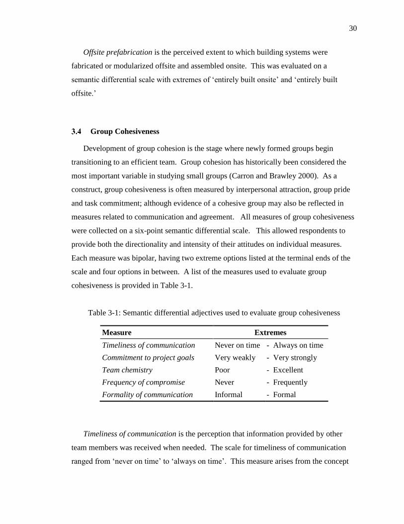
30
Offsite prefabrication is the perceived extent to which building systems were
fabricated or modularized offsite and assembled onsite. This was evaluated on a
semantic differential scale with extremes of ‘entirely built onsite’ and ‘entirely built
offsite.’
Group Cohesiveness
Development of group cohesion is the stage where newly formed groups begin
transitioning to an efficient team. Group cohesion has historically been considered the
most important variable in studying small groups (Carron and Brawley 2000). As a
construct, group cohesiveness is often measured by interpersonal attraction, group pride
and task commitment; although evidence of a cohesive group may also be reflected in
measures related to communication and agreement. All measures of group cohesiveness
were collected on a six-point semantic differential scale. This allowed respondents to
provide both the directionality and intensity of their attitudes on individual measures.
Each measure was bipolar, having two extreme options listed at the terminal ends of the
scale and four options in between. A list of the measures used to evaluate group
cohesiveness is provided in Table 3-1.
Table 3-1: Semantic differential adjectives used to evaluate group cohesiveness
Measure Extremes
Timeliness of communication Never on time - Always on time
Commitment to project goals Very weakly - Very strongly
Team chemistry Poor - Excellent
Frequency of compromise Never - Frequently
Formality of communication Informal - Formal
Timeliness of communication is the perception that information provided by other
team members was received when needed. The scale for timeliness of communication
ranged from ‘never on time’ to ‘always on time’. This measure arises from the concept
31
of information latency, the lag between when a team member requests information and
receives a useful response. Lower latency is associated with higher team satisfaction and
reduced schedule durations on projects using an integrated design process (Chachere et
al. 2008).
Commitment to project goals is the perceived extent to which all team members were
committed to the same project goals, evaluated on a scale between ‘very weakly’ and
‘very strongly’. Goal commitment is directly analogous to task commitment as a
measure of group cohesiveness (Zaccaro and McCoy 1988). Commitment is influenced
by the team’s belief in the importance of project outcomes and that the goals are
realistically attainable (Locke and Latham 2002).
Team chemistry is the perception of compatibility among team members, arising from
differences in personalities and past and present relationships. This measure originated in
prior project delivery research (Konchar 1997), and the scale of team chemistry ranged
from ‘poor’ to ‘excellent’. Conceptually, team chemistry closely aligns with
intrapersonal attraction (Festinger et al. 1950) and group pride (Bollen and Hoyle 1990)
in group cohesiveness literature.
Frequency of compromise is the perceived prevalence of compromises being made
within the project team, evaluated on a scale between ‘never’ and ‘frequently’. To
compromise, the project team must collaborate to find a mutually acceptable solution that
satisfies all parties. This measure is new to construction research, although the concept
of compromise and the balance between cooperation and competition are studied in the
field of game theory.
Formality of communication is the perceived extent to which the project team
engages in brief, impromptu interaction or more structured, prescribed channels. The
scale for formality of communication ranged from ‘informal’ to ‘formal.’ Informal
communication is viewed as an important mechanism for team members to exchange
information interactively and without being scheduled (Kraut et al. 2002). Conversely,

32
formal communication is typically one-way and follows a preset agenda with a planned
list of participants. Both forms of communication have a role on construction projects,
but informal interactions are believed to be more supportive of inter-organizational
relationships.
Project Performance
Every owner views project performance relative to their own project goals. An owner
on a new data center project with aggressive time to market expectations may place
greater emphasis on delivery speed, regardless of the extra cost needed for overtime or
tenant revisions made near project completion. Therefore, there is no single measure of
performance that is applicable for all building owners. Eight metrics were selected to
represent cost, schedule and quality performance in this research. The data used to
formulate these metrics was collected after project completion.
3.5.1 Cost Metrics
Costs were defined from the owner’s perspective and were representative of the
contractual commitments made for design and construction services. All costs were
reported in U.S. dollars and did not include the value of land, permitting fees or furniture,
fixtures and equipment. Cost data was used to create three performance metrics,
including unit cost, cost growth and intensity.
Unit cost is the cost of a building, relative to its size. Unit cost is expressed in dollars
per square foot and was calculated by Equation 3-2. Final project cost was the sum of
design and construction contracts at the completion of the project and facility size was the
gross square foot area of the building, including both occupied and unoccupied space.
The location factor was necessary to compare projects built in different cities throughout
the U.S., each with regionally varying labor and material costs. Location factors were
obtained from the 2014 RSMeans guidebook and were used to adjust each project’s costs
to the nationwide average. A time modifier was needed to compare projects built in

33
different years, under varying economic conditions. The Building Cost Index (BCI),
published each month by the Engineering News Record (ENR), was used to translate
completed project costs to current dollars. The time modifier is a dimensionless measure
represented Equation 3-2a. BCI June 2014 was the most recent BCI published at the
time of data cleaning and preparation. BCI Construction start was the historical BCI for
the month and year when construction began on each project in the data set. The
resulting time modifier adjusts for material and labor cost inflation between the time of
construction and present, allowing unit costs to be compared fairly across projects.
𝑈𝑛𝑖𝑡 𝑐𝑜𝑠𝑡 = 𝐹𝑖𝑛𝑎𝑙 𝑝𝑟𝑜𝑗𝑒𝑐𝑡 𝑐𝑜𝑠𝑡
𝐹𝑎𝑐𝑖𝑙𝑖𝑡𝑦 𝑠𝑖𝑧𝑒 × 𝐿𝑜𝑐𝑎𝑡𝑖𝑜𝑛 𝑓𝑎𝑐𝑡𝑜𝑟 × 𝑇𝑖𝑚𝑒 𝑚𝑜𝑑𝑖𝑓𝑖𝑒𝑟 (3-2)
𝑇𝑖𝑚𝑒 𝑚𝑜𝑑𝑖𝑓𝑖𝑒𝑟 = 𝐵𝐶𝐼𝐽𝑢𝑛𝑒 2014
𝐵𝐶𝐼𝐶𝑜𝑛𝑠𝑡𝑟𝑢𝑐𝑡𝑖𝑜𝑛 𝑠𝑡𝑎𝑟𝑡 (3-2a)
The second cost metric, cost growth, is the percent change in design and construction
costs over the duration of the project. Cost growth is expressed as a percentage and was
calculated with Equation 3-3. Actual project costs are the final design and construction
costs reported at the completion of the project. Planned project costs are the initial or
starting values of the contracts for design and construction services. Since cost growth is
dimensionless, no location or time adjustments were performed.
𝐶𝑜𝑠𝑡 𝑔𝑟𝑜𝑤𝑡ℎ = 𝐴𝑐𝑡𝑢𝑎𝑙 𝑝𝑟𝑜𝑗𝑒𝑐𝑡 𝑐𝑜𝑠𝑡 – 𝑃𝑙𝑎𝑛𝑛𝑒𝑑 𝑝𝑟𝑜𝑗𝑒𝑐𝑡 𝑐𝑜𝑠𝑡
𝑃𝑙𝑎𝑛𝑛𝑒𝑑 𝑝𝑟𝑜𝑗𝑒𝑐𝑡 𝑐𝑜𝑠𝑡 × 100 (3-3)
Lastly, intensity is a hybrid cost and schedule metric that examines the unit cost
installed per month of project duration. Intensity is expressed in dollars per square foot
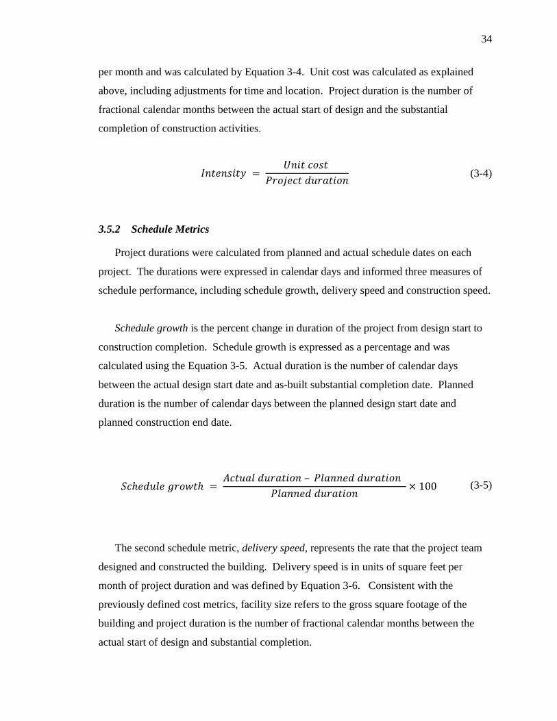
34
per month and was calculated by Equation 3-4. Unit cost was calculated as explained
above, including adjustments for time and location. Project duration is the number of
fractional calendar months between the actual start of design and the substantial
completion of construction activities.
𝐼𝑛𝑡𝑒𝑛𝑠𝑖𝑡𝑦 = 𝑈𝑛𝑖𝑡 𝑐𝑜𝑠𝑡
𝑃𝑟𝑜𝑗𝑒𝑐𝑡 𝑑𝑢𝑟𝑎𝑡𝑖𝑜𝑛 (3-4)
3.5.2 Schedule Metrics
Project durations were calculated from planned and actual schedule dates on each
project. The durations were expressed in calendar days and informed three measures of
schedule performance, including schedule growth, delivery speed and construction speed.
Schedule growth is the percent change in duration of the project from design start to
construction completion. Schedule growth is expressed as a percentage and was
calculated using the Equation 3-5. Actual duration is the number of calendar days
between the actual design start date and as-built substantial completion date. Planned
duration is the number of calendar days between the planned design start date and
planned construction end date.
𝑆𝑐ℎ𝑒𝑑𝑢𝑙𝑒 𝑔𝑟𝑜𝑤𝑡ℎ = 𝐴𝑐𝑡𝑢𝑎𝑙 𝑑𝑢𝑟𝑎𝑡𝑖𝑜𝑛 – 𝑃𝑙𝑎𝑛𝑛𝑒𝑑 𝑑𝑢𝑟𝑎𝑡𝑖𝑜𝑛
𝑃𝑙𝑎𝑛𝑛𝑒𝑑 𝑑𝑢𝑟𝑎𝑡𝑖𝑜𝑛× 100 (3-5)
The second schedule metric, delivery speed, represents the rate that the project team
designed and constructed the building. Delivery speed is in units of square feet per
month of project duration and was defined by Equation 3-6. Consistent with the
previously defined cost metrics, facility size refers to the gross square footage of the
building and project duration is the number of fractional calendar months between the
actual start of design and substantial completion.

35
𝐷𝑒𝑙𝑖𝑣𝑒𝑟𝑦 𝑠𝑝𝑒𝑒𝑑 = 𝐹𝑎𝑐𝑖𝑙𝑖𝑡𝑦 𝑠𝑖𝑧𝑒
𝑃𝑟𝑜𝑗𝑒𝑐𝑡 𝑑𝑢𝑟𝑎𝑡𝑖𝑜𝑛 (3-6)
Construction speed is rate that the building was constructed, as square feet per month
of construction duration. The method for calculating construction speed is provided in
Equation 3-7. Construction duration is the number of calendar months between the actual
start of construction and the construction substantial completion date.
𝐶𝑜𝑛𝑠𝑡𝑟𝑢𝑐𝑡𝑖𝑜𝑛 𝑠𝑝𝑒𝑒𝑑 = 𝐹𝑎𝑐𝑖𝑙𝑖𝑡𝑦 𝑠𝑖𝑧𝑒
𝐶𝑜𝑛𝑠𝑡𝑟𝑢𝑐𝑡𝑖𝑜𝑛 𝑑𝑢𝑟𝑎𝑡𝑖𝑜𝑛 (3-7)
3.5.3 Quality Metrics
Quality measures were obtained by asking the owner to rate, relative to their
expectations, aspects of the facility turnover experience and quality of installed building
systems. The measures related to the facility turnover experience included difficulty of
facility start-up, number and magnitude of call backs and operation and maintenance
(O&M) costs. Building system measures included the quality of envelope and structure,
interior finishes, environmental systems, the exterior aesthetic and interior environment.
Similar to the assessment of group cohesiveness, these quality measures were collected
on six-point semantic differential scale with extreme values of ‘Low’ and ‘High’. This
method of measuring project quality is subjective and does not assess the quality of work
directly; instead it reflects the owner’s satisfaction with a project that either met or failed
to meet expectations. There are no widely accepted equations for aggregating quality
measures, so this research uses an exploratory factor analysis to determine if latent
constructs of turnover experience and system quality may be represented by their
respective rating measures.

36
3.6 Programming Factors
Construction projects are delivered according to a scope of work or ‘program’ made
during the pre-design phases of the project. This program will outline the primary uses of
the building and targeted square footage of occupied space, as well as any special
requirements from the owner. These decisions made during programming persist
throughout design and construction, and are likely to influence the quality of inter-
organizational relationships and project performance. For example, a larger facility is
likely to require more coordination between trade contractors than a smaller building. A
public owner using government funding may institute stricter reporting policies for the
project team and create an additional administrative burden. Three programming factors
are identified in the theoretical framework, although only two are considered in the
analysis: owner type, facility size and facility type.
3.6.1 Owner Type
The owner type is categorized as either public or private, depending on the funding
source of the project. Publically funded projects are delivered by owners within or
receiving funding from local, state and federal government agencies. They are often
constrained by jurisdictional procurement laws when selecting project team members.
For example, projects receiving public funding may be required to select contractors
based solely on cost of work in response to greater financial scrutiny.
3.6.2 Facility Size
The size of a facility is the gross square foot area, which includes both occupied and
unoccupied space. Larger projects may benefit from improved productivity due to
reaching the plateau on the learning curve, and transitioning that experience to the next
floor or wing of the building. Larger projects also distribute fixed costs over a greater
number of units, resulting in economies of scale and reduced unit costs for building
systems. However, large projects are often more technically and organizationally
37
complex, and require more frequent team interaction to manage the additional
complexity.
3.6.3 Facility Type
The facility type is a categorization that describes the predominant use of the
building. Project complexity is often related to facility type. For instance, hospitals are
more technically complex than simple offices, with environmental systems that are more
challenging to design and construct. In this research, specific building uses were reduced
to a list of nine facility types, adapted from the U.S. Census Bureau’s classification of
non-residential buildings (U.S. Census Bureau 2014). As shown in Table 3-2,
commercial facilities included all retail and wholesale buildings, department stores and
service centers. Lodging included hotels, motels, resort lodging, military barracks and
dormitories. Offices represented administrative and professional buildings, as well as
banks. Correctional facilities included prisons and jails. Educational included K-12
schools, university classrooms and research labs, museums and libraries. Manufacturing
contained facilities for food processing, factory work and fabrication. Sports and
recreation included movie theaters, stadiums, community centers, convention center and
casinos. Transportation was composed of airport and bus terminals, and healthcare
included hospitals, clinics, medical offices, medical labs and nursing homes. While
facility type is explicitly mentioned in the theoretical framework, these classifications are
not modeled in the statistical analysis. A very large sample size would be needed to
observe significant differences in performance between nine facility types.
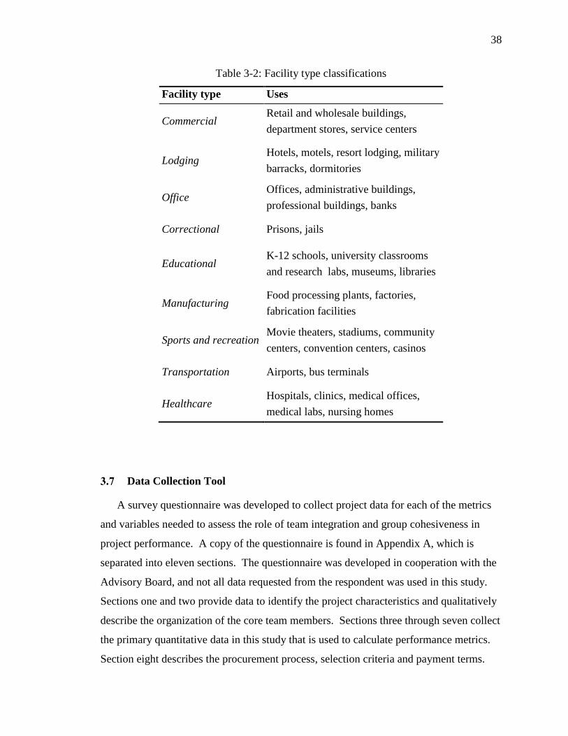
38
Table 3-2: Facility type classifications
Facility type Uses
Commercial Retail and wholesale buildings,
department stores, service centers
Lodging Hotels, motels, resort lodging, military
barracks, dormitories
Office Offices, administrative buildings,
professional buildings, banks
Correctional Prisons, jails
Educational K-12 schools, university classrooms
and research labs, museums, libraries
Manufacturing Food processing plants, factories,
fabrication facilities
Sports and recreation Movie theaters, stadiums, community
centers, convention centers, casinos
Transportation Airports, bus terminals
Healthcare Hospitals, clinics, medical offices,
medical labs, nursing homes
Data Collection Tool
A survey questionnaire was developed to collect project data for each of the metrics
and variables needed to assess the role of team integration and group cohesiveness in
project performance. A copy of the questionnaire is found in Appendix A, which is
separated into eleven sections. The questionnaire was developed in cooperation with the
Advisory Board, and not all data requested from the respondent was used in this study.
Sections one and two provide data to identify the project characteristics and qualitatively
describe the organization of the core team members. Sections three through seven collect
the primary quantitative data in this study that is used to calculate performance metrics.
Section eight describes the procurement process, selection criteria and payment terms.
39
Sections nine and ten include questions related to the team’s development and use of
high-quality interactions, respectively. Lastly, section eleven allowed the respondent to
comment on any lessons learned from the project and describe any unique features that
may have influenced its performance.
3.7.1 Pilot Testing
The survey questionnaire underwent both internal and external pilot testing prior to
distribution. The purpose of these tests was to (1) verify the availability of information
being requested in the questionnaire and (2) identify potential misunderstandings in the
wording of specific questions. The first draft of the questionnaire included
approximately 275 questions, or nearly three times the data points of similar project
delivery studies. Several redundant and onerous questions with little analytical value
were eliminated to reduce the likelihood of respondent fatigue lowering the quality of
data. The internal pilot included four projects, where a paper-based version of the
questionnaire was completed by contacting the project owner via phone and conducting a
survey-style interview. The external pilot was a test of both the survey distribution
methodology and an electronic, web-based version of the questionnaire. A letter of
introduction to the study and a web-link for the questionnaire were distributed via email
to a small sampling of industry contacts. The external pilot produced twelve responses
for ten unique projects. The most common feedback from participating owners and
contractors addressed the length of the questionnaire, which was universally viewed as
too time consuming. In response to this concern, a list of required ‘key project
information’ was added to the introductory letter, allowing respondents to search for and
obtain specific cost or schedule data prior to starting the questionnaire. Additionally, the
external pilot revealed the need for a verification step after receiving a completed
questionnaire. For example, the data for ‘total project cost’ was initially inconsistent,
despite explicitly stating in the question statement to exclude all property, process and
manufacturing equipment and furnishings costs. This verification was performed with a
follow-up phone call between the respondent and a member of the research team.
40
3.7.2 Section 1: Project Characteristics
Project identifier information, including the project name, location and respondent’s
contact details were collected in Section one. This data was kept confidential within the
research team. The project name was only used for reference during follow-up
conversations with the respondent and to avoid duplicating project entries in the database.
Respondents classified the owner as either public or private, and provided a brief
description of the intended use of the facility. Physical characteristics of the building,
including size, number of floors, foundation type and the percentage of new and
renovation work were also requested.
3.7.3 Section 2: Project Organization
Sections two asked the respondent to select the delivery method that most resembled
the delivery of their project. The possible selections included design-bid-build,
construction manager at risk, design-build and integrated project delivery. Additionally,
the timing of contract for each core team member was requested as a percentage of
overall design completion.
3.7.4 Section 3: Project Cost
Total project costs and construction only costs at contract award and final completion
were collected in Section three. The total project costs included both the design and
construction contract commitments, without the value of land, permitting fees or
furniture, fixtures and equipment. Costs at contract award represent the agreed upon
price from the designer or contractor for the initial scope of work. Costs at final
completion capture any changes or modifications to the contract values occurring during
the project. In cases where questionnaires were returned by contractors or construction
managers, the project owner was contacted to validate total project costs.
41
3.7.5 Section 4: Project Schedule
In Section four, respondents were asked to provide the planned and actual schedule
dates for the start of design, start of construction and substantial completion. A complete
date included the month, day and year. In cases where the respondent only provided a
month and year, the midpoint of the given month was used in duration calculations.
3.7.6 Section 5: Project Quality
Section five was only answered by the project owner. If the questionnaire was
returned by a designer or contractor, the name and phone number or email address of the
owner was requested. The owner was then contracted during the verification process to
complete this section. Measurements of quality were split into two subsections. The first
asked the owner to rate the facility turnover and operation, with respect to difficulty of
start-up, magnitude of call backs and operation and maintenance costs. The second
section asked the owner to evaluate quality of facility’s systems, including the structure
and envelope, interior finishes, environmental systems, exterior aesthetic and interior
environment.
3.7.7 Section 6: Project Safety
Section six was only answered by the primary contractor. If the questionnaire was
returned by a designer or owner, the name and phone number or email address of the
primary contractor was requested. This section asked the contractor to provide the total
number of recordable injuries and lost time injuries on the job, with an estimate of the
total labor hour for onsite construction activities. Section six data was collected, but not
analyzed in this phase of research.
3.7.8 Section 7: Sustainability
Section seven collected data on any green or sustainable rating system used on the
project. If a level of certification was obtained, respondents were asked to specify the

42
level planned during design and the level awarded after construction. Section seven data
was collected, but not analyzed in this phase of research.
3.7.9 Section 8: Team Procurement and Contracts
Information on how proposals were solicited for each team member, the selection
criteria for making the contract award and the resulting contract payment terms was
collected in Section 8. The options for proposal solicitation included open bid,
prequalified bid, single-stage request for proposal (RFP), 2-stage RFP and sole source.
Selection criteria were presented as a multiple select question, allowing the respondent to
indicate any combination of cost of work, cost of fees and general conditions, technical
proposal, design concept, similar project experience and interview performance. Lastly,
payment terms were indicated as lump sum, guaranteed maximum price (GMP) or cost
plus a fee.
3.7.10 Section 9: Team Characteristics and Behavior
Section nine asked the respondent to assess the level of team development on the
project, with specific emphasis on group cohesion. Several theorized indicators of group
cohesiveness were rated on a semantic differential scale, including chemistry, formality
and timeliness of communication, frequency of compromise and goal commitment. This
section also included data on co-location, the use of a shared design and construction
contingency and the team members participating in joint goal setting.
3.7.11 Section 10: Process and Technology
Details on the types of inter-organizational activities engaged in by the project team
were collected in Section ten. These included the number of design charrettes held, types
of BIM applications and the specific team members that were invited to participate.
Participation was presented as a series of multiple select questions, allowing the
respondent to indicate any combination of participating organizations from a list of the
owner, designer, construction manager or general contractor, MEP trades and structural

43
trades. A multiple select was also used to indicate the number of BIM application on the
project from a list of architectural design, engineered system design, MEP coordination,
4D scheduling and facility management. An evaluation for the level offsite
prefabrication was also included in this section.
3.7.12 Section 11: Lessons Learned
The last section allowed respondents to list specific suggestions for how the project
could have been delivered more successfully. Respondents were also asked to describe
any unique features or conditions that may have influenced the final cost, schedule or
quality performance.
Chapter Summary
A theoretical framework for studying inter-organizational relationships on
construction projects was developed using literature, related studies and industry
feedback. The framework informed a data collection instrument and provided the
structure for a statistical analysis of the data set. The specific methodologies of data
collection, verification and analysis are described in Chapter 4.

44
Chapter 4
DATA COLLECTION AND ANALYSIS METHODS
The purpose of this research was to explore relationships among team integration,
group cohesiveness and project performance within the context of project organizations.
To collect a broad range of quantitative project data, a survey questionnaire was
distributed to owners and contractors in the construction industry. Once responses were
received, they were checked for accuracy using a verification process and the data was
screened prior to analysis. Multivariate statistical methods, including latent class analysis
and structural equation modeling, were used to analyze the sample data set. This chapter
describes the data collection process and summarizes the analysis techniques used in
fulfillment of the research purpose.
Data Collection Methods
This research used a structured survey questionnaire to collect project information
directly from the project participants. As mentioned previously, the data collection effort
was performed in collaboration with the University of Colorado Boulder. Questionnaires
were distributed by postal mail and email to professional organizations in the
architecture, engineering and construction (AEC) industry. Because not all respondents
have the same knowledge of the project, a verification procedure was followed to confirm
key data with the project owner. Once verified by a member of the Penn State or
University of Colorado research team, project data was entered into an electronic
database and later screened to ensure a meaningful analysis. These steps in the data
collection methodology, which will be discussed in subsequent sections, are summarized
in Table 4-1.

45
Table 4-1: Summary of data collection methodology
Data Collection Method Description
1. Survey distribution PDF form for email distribution
Double-sided paper version for postal distribution
Surveys reached the following groups:
– Construction Owners Association of American (COAA)
– Design-Build Institute of American (DBIA)
– Construction Management Association of America (CMAA)
– Penn State University, AE Dept. Alumni (1976-2012)
– Penn State University, PACE (2012-2013)
2. Data recording and
verification
Data recorded into single database
Completed surveys reviewed and annotated for verification
Verification performed by research assistants at Penn State
University and the University of Colorado Boulder
3. Data screening Combined multiple responses into single database entry
Removed projects outside the study scope
Removed unverified projects
Check data assumptions for statistical analysis
4.1.1 Survey Distribution
After developing and piloting the survey questionnaire, the document was distributed
to the study’s targeted population of project participants. Since a truly simple random
sample of recently completed construction projects was not feasible, this research sought
a large-scale convenience sample. Mailing lists from professional, alumni and academic
organizations were used to reach a diverse group of project participants. Respondents
were asked to complete the survey for their most recently completed project. The survey
was intended primarily for owners, as the party with the most complete knowledge of the
project; however contractors, construction managers and designers were not discouraged
from participating. Surveys were sent as a PDF form for email distributions and as a
double-sided paper version for postal mailings. Both forms of distribution were
accompanied by a cover letter and list of frequently asked questions (FAQs) that
explained the purpose of the study and listed definitions for several key terms.

46
Respondents that received the PDF form had the option of printing the survey and
answering by hand, or completing the form electronically.
Approximately 2,500 surveys were sent via postal mail to alumni of the Architectural
Engineering Department at Penn State and 41 were returned, representing a 1.6%
response rate. Nearly 6,000 surveys were distributed by email to mailing lists for the
Construction Owners Association of American (COAA), Design-Build Institute of
American (DBIA), Construction Management Association of America (CMAA) and the
Partnership for Achieving Construction Excellence (PACE) at Penn State. The research
team received 290 returned surveys from the email distribution, representing a 4.8%
response rate. When combined, a total of 331 surveys were received for this study,
resulting in a 3.9% overall response rate.
4.1.2 Data Recording and Verification
A Microsoft Access® database was developed to enter and store completed survey
responses. Forms were created with pull down menus, multiple select boxes and rating
scales that automatically coded the data into tables. This reduced the likelihood of
human error when manually entering data. Before each survey response was added to the
database, the project was assigned a unique identification number that included the
respondent’s role in the project and the initials of the research assistant tasked with data
verification. While research assistants were initially allowed to enter data directly into
concurrent versions of databases, access was later centralized into a single database and
restricted to senior researchers only.
The following procedures were used to verify the project information in returned
surveys. First, returned surveys were reviewed for missing and inconsistent data. If
necessary, annotations with clarifying questions or lines of further inquiry were attached
to the survey. Special scrutiny was given to contract values and schedule dates to
improve the accuracy of outcome data. This screening and annotation process ensured
that interactions with survey respondents were consistent and professional. Data

47
verification was conducted with follow-up phone calls and emails made by research
assistants at Penn State and the University of Colorado Boulder. Each assistant was
familiarized with the objectives of the research and made aware of the terminology used
in the survey. Assistants were trained in verification procedures by observing and
participating in several follow-up calls made by a senior researcher. In cases where the
survey respondent was not the project owner, the owner was contacted to obtain quality
measures and verify cost and schedule data.
4.1.3 Data Screening
Data screening was performed to prepare the sample data for analysis. First, the
database tables were exported directly to a Microsoft Excel® spreadsheet. Cells with
missing data were coded as -99999 to alert analysis programs to exclude those values.
Projects with over 30% missing data across the study variables were removed. Columns
were added and calculated for performance metrics using the verified costs and schedule
dates. Projects that were outside the scope of this research were removed from the
spreadsheet. These included renovation project with less than 50% new construction by
cost, international projects, civil and highway work, uncompleted projects, facilities less
than 5,000 gross square feet and projects completed prior to 2008. Additionally, several
projects were not validated with the owner due to non-response from the point of contact.
Projects with more than one respondent (e.g. an owner and contractor submitting a
survey for the same project) were combined into a single case. A multi-step procedure
was followed for resolving discrepancies among respondent (Table 4-2). For quantitative
data, including contract values and schedule dates, the first action is a follow-up
discussion with the respondents to verify the data source or confirm that the question was
fully understood by the respondent. If a follow-up was not possible or unsuccessful in
resolving the conflict, then values marked as ‘Actual’ by a single respondent or the more
precise value from multiple respondents was entered. For qualitative data with nominal
categories, the study definitions were used to re-classify conflicting responses, after
verifying that each term was understood by the respondents. For qualitative data derived

48
from ordinal scales, the mean rating of all project respondents was used, with the
exception of quality ratings. All quality rating reflected only the opinions of the project
owner.
Table 4-2: Actions for resolving multiple response discrepancies
Data Type Research Actions
Step 1 Step 2 Step 3
Quantitative Verify source data
with respondent
Preference to data
denoted as ‘Actual’
Preference to
precise data,
otherwise use mean
Qualitative (Nominal)
Verify terms were
understood by
respondent
Re-classify response
using study
definitions ---
Qualitative (Ordinal) Preference to owner
(e.g. Quality ratings)
Enter mean rating
across all respondents ---
Lastly, the data screening process examined descriptive statistics for each observed
variable. Specifically, the means, medians, minimums and maximums were reviewed for
any out-of-range values as well as potential data entry errors. Additionally, the
distributions of continuous and ordered categorical variables were considered. Most
continuous variables were found to have some degree of skewness and kurtosis, and did
not follow a normal distribution. A procedure for transforming non-normal data is
discussed alongside the data analysis methods. Several ordered categorical variables
were collapsed to consolidate response options with a low number of observations. Since
analyses involving categorical variables proceed from a frequency or cross-tabulation
table, response options with zero or few observations can lead to difficulty in estimation
(Bentler and Chou 1987). Therefore, the measurement scales of group cohesiveness
measures were collapsed from six points to either four or five points. In all cases,
collapsing response options eliminated a positive or negative tail in the distributions
toward one of the extremes. The lower extremes of the scales for timeliness of
communication, commitment to project goals and team chemistry were collapsed to
produce a new four point scale. Conversely, the upper extremes of the scales for
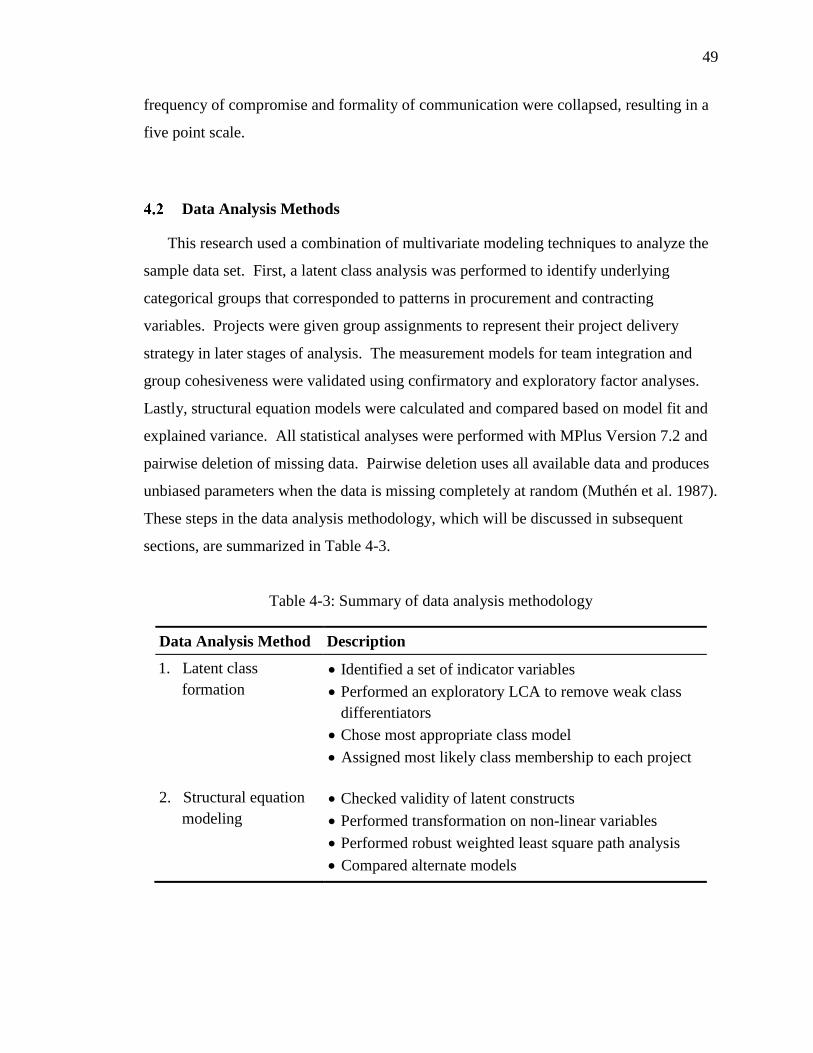
49
frequency of compromise and formality of communication were collapsed, resulting in a
five point scale.
Data Analysis Methods
This research used a combination of multivariate modeling techniques to analyze the
sample data set. First, a latent class analysis was performed to identify underlying
categorical groups that corresponded to patterns in procurement and contracting
variables. Projects were given group assignments to represent their project delivery
strategy in later stages of analysis. The measurement models for team integration and
group cohesiveness were validated using confirmatory and exploratory factor analyses.
Lastly, structural equation models were calculated and compared based on model fit and
explained variance. All statistical analyses were performed with MPlus Version 7.2 and
pairwise deletion of missing data. Pairwise deletion uses all available data and produces
unbiased parameters when the data is missing completely at random (Muthén et al. 1987).
These steps in the data analysis methodology, which will be discussed in subsequent
sections, are summarized in Table 4-3.
Table 4-3: Summary of data analysis methodology
Data Analysis Method Description
1. Latent class
formation
Identified a set of indicator variables
Performed an exploratory LCA to remove weak class
differentiators
Chose most appropriate class model
Assigned most likely class membership to each project
2. Structural equation
modeling
Checked validity of latent constructs
Performed transformation on non-linear variables
Performed robust weighted least square path analysis
Compared alternate models

50
4.2.1 Latent Class Formation
Latent class analysis (LCA) uses a clustering algorithm to identify underlying,
categorical subgroups or ‘classes’ in a sample. Classes are defined by the presence or
absence of indicators, expressed as a probability, that differentiate one class from
another. The purpose of this analysis was to better represent the construction project as
an organization, using variables known to impact the structure of project team.
Unordered categorical variables for procurement and contracting were reduced to binary
indicators. Multiple class models were formed and based on fit and selection indices, the
appropriate number of classes was chosen to represent the data. Lastly, each project was
assigned to the class with its highest probability of belonging.
4.2.2 Structural Equation Modeling
Several estimation methods may be used with structural equation modeling (SEM) to
obtain coefficients, standard errors and fit indices. As with most statistical techniques,
SEM makes assumptions that should be satisfied before trusting the results of an analysis.
For the most common types of estimators, maximum likelihood (ML) and generalized
least square (GLS), the following assumptions are made regarding the sample data (Kline
2011):
1. The observations are independent and unstandardized;
2. The joint distribution of observed variables is multivariate normal, implying that
the observed variables are also continuous; and
3. The independent variables are measured without error.
For this research, the assumption of multivariate normality was not satisfied.
Specifically, measures accounting for variations in facility size were positively skewed
with very high kurtosis. This included facility size, unit cost, delivery speed,
construction speed and intensity. Since the sample included facility sizes over many
orders of magnitude, ranging from 5,000 square feet to over 1-million, these measures
were transformed with a base 10 logarithm. The transformed metrics followed a normal

51
distribution with both skewness and kurtosis falling between -1 and 1. Additionally, this
research used ordered categorical data in the same model as continuous data. Ordered
categorical data is discrete in nature and cannot be normally distributed, failing to satisfy
the multivariate normality assumption. Using this type of data in maximum likelihood
estimation has documented effects in SEM, including (1) underestimation of fit indices
suggesting that a correctly specified model does not fit the data (Hutchinson and Olmos
1998) and (2) a negative bias in regression parameters with increased standard errors
(Babakus et al. 1987; Muthén and Kaplan 1985). Since the sample data did not satisfy
the model assumptions needed for ML or GLS estimation, this research employed a mean
and variance adjusted weighted least square estimator (WLSMV).
WLSMV estimation incorporates extra non-negative constants, or ‘weights’, for each
parameter during the fitting process. Of the estimators suitable for analyzing non-normal
categorical data, WLSMV was found to perform the best in SEM applications (Brown
2006). The weights are derived from the diagonals of the covariance matrix of parameter
estimates. In other words, parameters that are more precise (i.e. having a lower variance)
are given more weight, and those with less precision are given less weight. The result is
a robust regression methodology that, when applied to correctly specified models,
provides unbiased parameter estimates for ordered categorical and non-normal data
(Muthén and Kaplan 1985).
Several structural models were developed to best arrange the study’s latent constructs
in relation to performance outcomes. These models were calculated with and without
control variables. Two indices were selected to assess model fit: the root mean square
error of approximation (RMSEA) and comparative fit index (CFI). RMSEA is a measure
of model misspecification that considers the number of variables in the model, and ranges
from values of 0 to 1. Well-fitting models have RMSEA less than .08 (Hooper et al.
2008). The CFI compares the specified model against a baseline model that assumes no
correlation among observed variables. The resulting index is a value between 0 and 1,
with values at .95 and above indicating a good fit (Hu and Bentler 1999). Additionally,
as a measure of variance explained in dependent variables, R2 was considered alongside
52
fit indices when choosing between alternate models. This additional criterion was
implemented to avoid situations where the best fit model would be selected over a good
fit model with better predictive ability.
Sources of Bias
Potential sources of bias in this research included the self-selection of projects by the
respondent and non-response from individuals declining to return the survey or the
implicit exclusion of projects not associated with individuals or organizations on the
selected mailing lists
4.3.1 Self-Selection Bias
Self-selection bias occurs if respondents demonstrated a preference for completing
the questionnaire with only poor or only favorable project experiences. Two measures
were taken to reduce this type of response bias. First, the instructions distributed with the
questionnaire explicitly requested a wide array of projects, both typical and challenging
to inform respondents that the study is not targeting a specific type of project or
performance outcome. Secondly, respondents were asked to rate the overall success of
the project. Self-section bias may also occur if a large number of projects are submitted
by a single respondent or organization (e.g. design-build projects from members of the
Design-Build Institute of America). To limit this type of bias, the total number of
projects submitted by any individual or organizational was limited to 10% of the total
sample size.
4.3.2 Non-Response Bias
Using a mailing list to distribute the questionnaire implicitly excludes those projects
without a team member represented in the mailing list. Therefore, the instructions also
include a request that respondents share the questionnaire with other individuals, both
inside and outside of their own company. This encouraged snowball or referral sampling,

53
which allowed respondents to recruit new groups of participants that may not have
received the initial distribution of the questionnaire.
Chapter Summary
A survey questionnaire was used to collect data from project participants. To ensure
the accuracy of data, a verification procedure was followed by the research team to
follow-up with each respondent. The data was screened for out-of-range values and the
distributions were checked for normality violations prior to analysis. The applicability of
multivariate analysis techniques, including latent class formation and SEM, were
discussed. Lastly, sources of self-selection and non-response bias were identified.
54
Chapter 5
LATENT CLASS MODEL OF DELIVERY
Chapter 5 begins with a discussion of latent class analysis and describes how the
procedure was used to identify underlying groups or “classes” of project delivery
strategies. Indicator variables of delivery strategies are then reviewed and narrowed
according to their strength as differentiators of latent classes. Multiple-class models are
compared using fit indices to select a single model that best represents the underlying
project delivery strategies found in the data set. Lastly, individual projects were assigned
to the class with the highest posterior probability, or likelihood of belonging.
Preparing for Latent Class Analysis
Latent class analysis (LCA) is a statistical method of identifying discrete subgroups
within multivariate response data. LCA posits that an underlying, categorical latent
variable is responsible for the variation in two or more observed variables. Similar in
concept to factor analysis, LCA is methodologically more akin to clustering analysis.
Whereas factor analysis is concerned with the structure of observed variables as
correlational, LCA is concerned with the structure of cases as taxonomical. Given a
sample of cases (respondents, projects, etc.) with several observed variables, LCA
determines if there is a clear separation of cases into a smaller number of subgroups.
These subgroups are referred to as “classes” and within each latent class, each observed
variable is assumed to be statistically independent of every other variable. Thus, the
latent class is assumed to account for all of the association between observed variables.
In this study, LCA is used to extract a small number of project delivery strategies
from patterns of organizational, procurement and contracting variables in the data set.
55
The primary goal for this stage of the research was to identify granularity in the broader
classification of project delivery methods that reflects real practices in the industry. The
secondary goal was to investigate a statistical method of data reduction to assist in the
identification of a structural path analysis. The steps in building a latent class model for
this research include:
1. Identify and code a set of indicator variables that may differentiate between classes
of project delivery strategies.
2. Perform an exploratory LCA to identify and remove weak indicator variables.
3. Choose the most appropriate model, with the least number of latent classes using
goodness-of-fit statistics (χ2, G2) and lowest information loss (AIC, BIC).
4. Use posterior probabilities to assign a class number to each response case.
5.1.1 Coding of Indicator Variables
Prior to performing the LCA, dichotomous indicator variables were identified from
several observed variables in the data set. The relevant observed variables were
categorical and described the organization, procurement and contracting of the project
team. Table 5-1 summarizes the classification of these nominal variables into
dichotomous, “Yes” or “No” indicators. For example, when the owner held a single
contract for design and construction services, as in design-build (DB) and integrated
project delivery (IPD), indicator D1 was coded as a “Yes” response. D1 was coded as
“No” when the contract arrangement was split, as found in design-bid-build (DBB) or
CM at risk (CMR). The remaining indicators D2-D13 were similarly coded to
differentiate between delivery strategies and meet the assumption of conditional
independence for LCA. Interviewing the primary contractor prior to selection (D10) and
the use of a shared design and construction contingency (D11) were already dichotomous
responses in the data set, and therefore not re-coded.

56
Tab
le 5
-1:
Dic
hoto
mous
clas
sifi
cati
ons
of
del
iver
y s
trat
egy i
ndic
ators
Dic
hoto
mou
s cl
ass
ific
ati
on
Yes
= D
B, IP
D;
No =
DB
B, C
MR
Yes
= S
D o
r ea
rlie
r
No =
DD
or
late
r
Yes
= P
QB
, 2
-Sta
ge
RF
P, S
S
No =
OB
, 1
-Sta
ge
RF
P
Yes
= C
ost
of
work
No =
Fee
and/o
r qual
ific
atio
ns
Yes
= G
MP
, C
PF
No =
LS
N/A
N/A
Yes
= R
epea
t
N
o =
Fir
st t
ime
Del
iver
y s
trate
gy i
nd
icato
r
Ow
ner
hel
d a
sin
gle
contr
act
for
des
ign a
nd c
onst
ruct
ion
Pri
mar
y b
uil
der
was
hir
ed d
uri
ng s
chem
atic
des
ign o
r ea
rlie
r
Tra
de
contr
acto
rs w
ere
hir
ed d
uri
ng s
chem
atic
des
ign o
r ea
rlie
r
Pri
mar
y b
uil
der
was
pre
qual
ifie
d
Tra
de
contr
acto
rs w
ere
pre
qual
ifie
d
Pri
mar
y c
ontr
acto
r w
as s
elec
ted b
ased
on c
ost
of
work
Tra
de
contr
acto
rs w
ere
sele
cted
bas
ed o
n c
ost
of
work
Pri
mar
y c
ontr
acto
r had
an o
pen
book c
ontr
act
Tra
de
contr
acto
rs h
ad o
pen
book c
ontr
acts
Pri
mar
y c
ontr
acto
r w
as i
nte
rvie
wed
pri
or
to s
elec
tion
Pro
ject
use
d a
shar
ed d
esig
n a
nd c
onst
ruct
ion c
onti
ngen
cy
Ow
ner
had
a p
rior
rela
tio
nsh
ip w
ith t
he
des
igner
Ow
ner
had
a p
rior
rela
tio
nsh
ip w
ith t
he
pri
mar
y c
ontr
acto
r
D1
D2
D3
D4
D5
D6
D7
D8
D9
D10
D11
D12
D13

57
A summary of the re-coded indicator variables is provided in Table 5-2, which lists
the frequencies of “Yes”, “No” and “Missing” responses for the sample (N=204).
Prequalification of the primary contractor (D4) and trade contractors (D5) were the most
common indicators at frequencies of 72% and 70%, respectively. Trade contractors
having an open book contract (D9) was the least common, with an occurrence of only
13% across all cases. There was very little missing data in these indicator variables. The
use of shared design and construction contingency (D11) had the highest frequency of
non-response at 6% across all cases. Taken in isolation, these item-response frequencies
are useful descriptors of the sample data set. However, further analysis using LCA is
used to identify common patterns of indicators that would more accurately capture
project delivery strategies in practice.
Table 5-2: Item-response frequencies for delivery strategy indicators
Frequency (N=204)
Delivery strategy indicator Yes No Missing
D1 Owner held a single contract for design and construction .41 .59 .00
D2 Primary builder was hired during SD or earlier .67 .33 .00
D3 Trade contractors were hired during SD or earlier .64 .36 .00
D4 Primary builder was prequalified .72 .27 .00
D5 Trade contractors were prequalified .70 .29 .00
D6 Primary contractor was selected based on cost of work .60 .39 .01
D7 Trade contractors were selected based on cost of work .71 .26 .03
D8 Primary contractor had an open book contract .54 .46 .00
D9 Trade contractors had open book contracts .13 .87 .00
D10 Primary contractor was interviewed prior to selection .55 .45 .00
D11 Project used a shared design and construction contingency .28 .66 .06
D12 Owner had a prior relationship with the designer .57 .39 .04
D13 Owner had a prior relationship with the primary contractor .56 .42 .01
58
5.1.2 Identifying Poor Differentiators
When using the complete list of delivery indicators (D1-D13) in exploratory three,
four and five-class models, several indicators were identified as poor differentiators of
latent class. The presence of open book contracts at the trade contractor level (D9) and
use of a shared design and construction contingency (D11) had probabilities less than 0.3
across all class models. This suggests that neither indicator occurs frequently on projects
and cannot serve as differentiator of delivery strategies. Similarly, the owner having a
prior working relationship with the designer (D12) and primary contractor (D13) had
probabilities between 0.4 and 0.6 across all class models. A probability around 0.5
suggests that these indicators may be independent of delivery strategy, since they occur
with nearly equal likelihood or unlikelihood within all classes. Lastly, the primary
contractor being interviewed prior to selection (D10) was redundant with the primary
contractor being selected based on cost of work (D6). This redundancy was evident in
each model, where classes with high probabilities of cost of work selection had
consistently low probabilities of contractor interviews. Therefore, the weak indicators
D9-D13 were removed from the LCA, and the class models were recalculated using only
the remaining, strong indicators D1-D8.
Comparing LCA Models
The LCA models were calculated using robust maximum likelihood estimation
(MLR) and were re-run a minimum of three times with varying random start values to
avoid local maxima solutions. All calculations were performed using the MPlus Version
7.2 statistical software package with the mixture model add-on. The outputs for an
analysis of a user-specified number of latent classes include: (1) model fit and selection
statistics, (2) conditional probabilities of a “Yes” response for each indicator in each
latent class, (3) posterior probabilities of class membership for each case, and (4) class
assignment for each case based on the highest posterior probability. The model fit
statistics compare observed and expected response patterns using chi-square (χ2) and
likelihood ratio tests (G2). These statistics test the null hypothesis that the observed
response frequency is equal to the expected frequency. Therefore, a low p-value and

59
rejection of the null hypothesis indicates a poor fitting latent class model. Selection
statistics combine goodness-of-fit with model complexity, using the maximized log-
likelihood to calculate Akaike Information Criterion (AIC) and Bayesian Information
Criterion (BIC). Chi-square tests are reasonable in assessing model fit for a LCA where
the sample size is large and the number of indicators is small. Similar to all cross-
tabulations, when there are too many sparse response patterns with low or zero
frequencies, the chi-square and likelihood ratio tests are not valid. Therefore, the best-fit
latent class model typically has the lowest AIC or BIC value of all the models considered.
Using the reduced indicator list (D1-D8), separate LCA models were created
iteratively for up to six classes. A summary of the fit indices, selection criterion and ratio
testing for each latent class solution are provided in Table 5-3. The one, two and three-
class solutions have significant χ2 and G2 statistics, which indicates a poor fit between the
response pattern of the indicator variables and those expected under the model.
Additionally, the Vuong-Lo-Mendell-Rubin (VLMR) likelihood ratio test was significant
in the one, two and three-class models. The VLMR test assesses the null hypothesis (H0)
that a lower number of classes, k – 1, are a better fit than the current number of classes, k.
Therefore, rejecting the null hypothesis for the one, two and three-class models, while
failing to reject the four and five-class models, suggests that the four-class solution is an
adequate fit. The AIC and sample-size adjusted BIC decrease as the number of latent
classes increases, but the rate of decline begins to taper off after the four-class model.
Based on these comparisons, the four and five-class solutions appear to strike the best
balance between model fit and complexity.
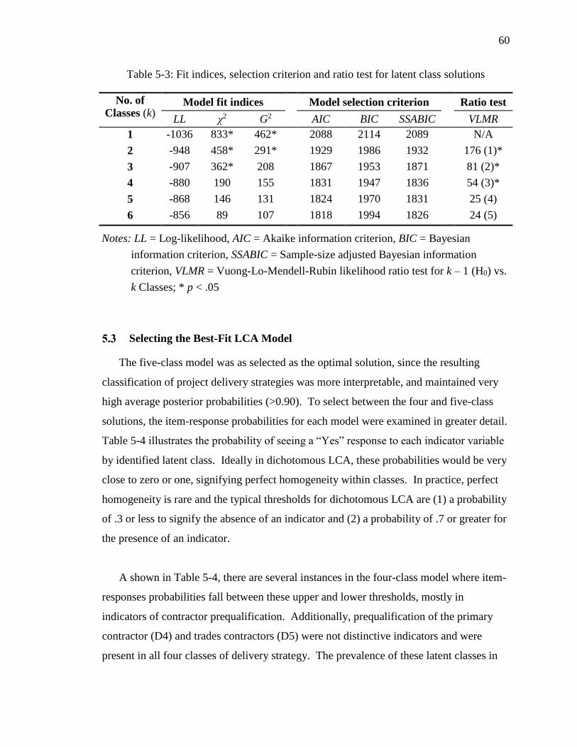
60
Table 5-3: Fit indices, selection criterion and ratio test for latent class solutions
No. of
Classes (k) Model fit indices Model selection criterion Ratio test
LL χ2 G2 AIC BIC SSABIC VLMR
1 -1036 833* 462* 2088 2114 2089 N/A
2 -948 458* 291* 1929 1986 1932 176 (1)*
3 -907 362* 208 1867 1953 1871 81 (2)*
4 -880 190 155 1831 1947 1836 54 (3)*
5 -868 146 131 1824 1970 1831 25 (4)
6 -856 89 107 1818 1994 1826 24 (5)
Notes: LL = Log-likelihood, AIC = Akaike information criterion, BIC = Bayesian
information criterion, SSABIC = Sample-size adjusted Bayesian information
criterion, VLMR = Vuong-Lo-Mendell-Rubin likelihood ratio test for k – 1 (H0) vs.
k Classes; * p < .05
Selecting the Best-Fit LCA Model
The five-class model was as selected as the optimal solution, since the resulting
classification of project delivery strategies was more interpretable, and maintained very
high average posterior probabilities (>0.90). To select between the four and five-class
solutions, the item-response probabilities for each model were examined in greater detail.
Table 5-4 illustrates the probability of seeing a “Yes” response to each indicator variable
by identified latent class. Ideally in dichotomous LCA, these probabilities would be very
close to zero or one, signifying perfect homogeneity within classes. In practice, perfect
homogeneity is rare and the typical thresholds for dichotomous LCA are (1) a probability
of .3 or less to signify the absence of an indicator and (2) a probability of .7 or greater for
the presence of an indicator.
A shown in Table 5-4, there are several instances in the four-class model where item-
responses probabilities fall between these upper and lower thresholds, mostly in
indicators of contractor prequalification. Additionally, prequalification of the primary
contractor (D4) and trades contractors (D5) were not distinctive indicators and were
present in all four classes of delivery strategy. The prevalence of these latent classes in

61
the sample data set ranges from a minimum of 19% for Class IV to a maximum of 28%
for Class I. Overall, the four-class model fits the data well, but struggles to differentiate
any group of projects without contractor prequalification.
Table 5-4: Item-response probabilities for the four-class solution
Latent class
I II III IV
Latent class prevalence in data set .28 .26 .26 .19
Item-response probabilities Probability of a Yes response
D1 Owner held a single contract for design and construction .09 .09 .89 .69
D2 Primary builder was hired during SD or earlier .00 .80 1.0 1.0
D3 Trade contractors were hired during SD or earlier .00 .07 .70 .84
D4 Primary builder was prequalified .64 .69 .84 .73
D5 Trade contractors were prequalified .62 .78 .76 .64
D6 Primary contractor was selected based on cost of work .93 .27 .90 .18
D7 Trade contractors were selected based on cost of work .76 .87 1.0 .10
D8 Primary contractor had an open book contract .23 1.0 .29 .70
Average posterior probability for classification .93 .96 .91 .96
Notes: Probabilities greater than .60 are highlighted to aid in interpretation. The probability
of a “No” response can be calculated by subtracting the item-response probabilities
shown above from 1.
However, when considering the five-class solution, there is a clear class of projects
without contractor prequalification. By expanding the model by an additional class,
Class I from the four-class model was split into two groups in the five-class model shown
in Table 5-5: Class I without any prequalification, and Class II with both primary
contractor (D4) and trade contractor prequalification (D5). While the comparison of fit
statistics suggested that the four-class solution was adequate in grouping project delivery
strategies, the five-class solution better aligns with literature on prequalification. Prior
studies consistently highlight the importance of examining contractor qualifications prior
to soliciting a proposal or bid (Russell et al. 1992; Palaneeswaran and Kumaraswamy
2001). Additionally, the five-class solution has more homogenous classes, with fewer

62
item-response probabilities falling in between the upper (.7) and lower (.3) thresholds. In
the sample data set, the prevalence of these classes ranges from a minimum of 9% for
Class I to a maximum of 27% for Class IV. Although the low representation of Class I in
the sample data set is not desirable, the recognition of prequalification as a class
differentiator makes the five-class model more reflective of practices in the construction
industry.
Table 5-5: Item-response probabilities for the five-class solution
Latent class
I II III IV V
Latent class prevalence in data set .09 .19 .26 .27 .18
Item-response probabilities Probability of a Yes response
D1 Owner held a single contract for design and construction .00 .13 .09 .90 .69
D2 Primary builder was hired during SD or earlier .00 .03 .80 1.0 1.0
D3 Trade contractors were hired during SD or earlier .00 .00 .07 .71 .84
D4 Primary builder was prequalified .03 1.0 .67 .84 .73
D5 Trade contractors were prequalified .32 .79 .78 .76 .64
D6 Primary contractor was selected based on cost of work .95 .92 .27 .90 .18
D7 Trade contractors were selected based on cost of work .85 .71 .88 1.0 .10
D8 Primary contractor had an open book contract .00 .34 1.0 .29 .70
Average posterior probability for classification .91 .96 .91 .94 1.0
Notes: Probabilities greater than .60 are highlighted to aid in interpretation. The probability
of a “No” response can be calculated by subtracting the item-response probabilities
shown above from 1.
A Five-Class Model of Project Delivery Strategies
Each of the five classes is described in Figure 5-1, using the estimated probabilities of
encountering each indicator variable on projects within a given class. The nomenclature
adopted for these classes reflects the combination of indicators with estimated
probabilities greater than 0.65 found in each class:

63
Class I: Projects in this class universally reported split design and construction
contracts (0.00 probability of a single contract), no early primary contractor (0.00)
and trade (0.00) involvement, a small probability of primary contractor
prequalification (0.03), a small probability of trade prequalification (0.32), very high
probabilities of primary contractor (0.95) and trades (0.85) being selected based on
cost of work, and no use of open book contracts (0.00). The prevalence of this class
in the data set was 9% (n=19).
Figure 5-1: Probabilities of having each indicator variable for the five latent classes
Class II: These projects reported a small probability of a single design and
construction contract (0.13), very small probabilities of early primary contractor
(0.03) and trade (0.00) involvement, universal prequalification of the primary
contractor (1.00), high probability of trade prequalification (0.79), very high
probabilities of primary contractor (0.92) and trades (0.71) being selected based on
cost of work, and a small probability of an open book contract with the primary
contractor (0.34). The prevalence of this class in the data set was 19% (n=39).
0.0
0.1
0.2
0.3
0.4
0.5
0.6
0.7
0.8
0.9
1.0
D1 D2 D3 D4 D5 D6 D7 D8
Est
ima
ted
Pro
ba
bil
ity
Indicator
Class I
Class II
Class III
Class IV
Class V

64
Class III: Projects in this class reported a small probability of a single design and
construction contract (0.09), very high probability of early primary contractor
involvement (0.80), very small probability of early trade involvement (0.07), high
probability of prequalification for the primary contractor (0.67) and trades (0.78),
small probability of the primary contractor being selected based on cost of work
(0.27), very high probability of trades being selected based on cost of work (0.88),
and universal use of an open book contract (1.00). The prevalence of this class in the
data set was 26% (n=54).
Class IV: This class was characterized by near universal use of a single design and
construction contract (0.90), universal early primary contractor involvement (1.00),
very high probability of early trade involvement (0.71), very high probability of
primary contractor (0.84) and trade (0.76) prequalification, near universal
consideration of cost of work when selecting the primary contractor (0.90) and trades
(1.00), and small probability of an open book contract (0.29). The prevalence of this
class in the data set was 27% (n=56).
Class V: These projects reported a high probability of a single design and
construction (0.69), universal early primary contractor involvement (1.00), very high
probability of early trade involvement (0.84), high probability of primary contractor
(0.73) and trade (0.64) prequalification, small probabilities of selecting the primary
contractor (0.18) and trades (0.10) based on cost of work, and very high probability of
an open book contract (0.70). The prevalence of this class in the data set was 18%
(n=36).
5.4.1 Class Assignment using Posterior Probabilities
Calculated alongside the LCA, posterior probabilities are used to assign class
membership to projects in the data set. Posterior probabilities reflect the likelihood of a
given case belonging to each latent class, based on the case’s response pattern on the
indicator variables. For example, a sample case with posterior probabilities of 0.05 on

65
Class I, 0.00 on Class II, 0.92 on Class III, 0.03 on Class IV and 0.00 on Class V almost
certainly belongs in Class III, with a very small possibility of being part of Class I and
Class IV. In this manner, class assignments were made for all cases in the sample data
set (N=204) according to their highest posterior probability in the five-class solution.
This method of class assignment, which removes the uncertainty in classification, does
introduce a small amount of measurement error into future analyses.
One method of examining how well cases have been classified in the latent class
analysis is to examine the model’s entropy (Celeuz and Soromenho 1996). Entropy is
calculated according to Equation 5-1, where �̂�𝑖𝑘 is the estimated posterior probability for
case i in class k. The function scales this summation for the sample size of n and a total
number of classes, K. Entropy is bounded between zero and one, with a value of one
indicating that all cases were perfectly classified. The entropy of the five-class model in
this research was .88, which indicates strong delineation between classes. In simulation
studies, latent class models with entropy greater than .80 were found to have low levels
of assignment error.
𝐸𝑛𝑡𝑟𝑜𝑝𝑦 = ∑ ∑ (−�̂�𝑖𝑘𝑘 ln �̂�𝑖𝑘)𝑖
𝑛 ln 𝐾 (5-1)
5.4.2 Detailed Description of Classes
The creation of dichotomous indicators from observed variables was needed to obtain
an interpretable latent class model. However, once cases in the data set are assigned to
their most likely class, the observed variables may be re-examined to better understand
the types of projects grouped within each class. Figure 5-2 summarizes the distribution
of timing of involvement, represented by the stages of building design, for the primary
contractor (D2) and trade contractors (D3). There is a clear progression of primary
contractor involvement, which transitions from the bidding phase in Class I (95% of

66
cases in class) to conceptual design and earlier in Class IV (86%) and Class V (86%).
The Class II group has no primary contractor involvement prior to design development,
whereas Class III has less than 20% of cases with the primary contractor involved after
schematic design. At the 2nd tier contractor level, which includes MEP and structural
trades, involvement during the bidding phase was common in Class I (100%), Class II
(67%) and Class III (50%) projects. Trades were involved earliest in Class IV, with 52%
hired during conceptual design or earlier, and Class V, with 86% hired in schematic
design or earlier.
Figure 5-2: Involvement for contractors based on posterior class assignments
0%
20%
40%
60%
80%
100%
PRE CONC SD DD CD BID
Per
cen
t o
f P
roje
cts
Class I (n=19)
0%
20%
40%
60%
80%
100%
PRE CONC SD DD CD BID
Per
cen
t o
f P
roje
cts
Class II (n=39)
0%
20%
40%
60%
80%
100%
PRE CONC SD DD CD BID
Per
cen
t o
f P
roje
cts
Timing of Involvement
Class III (n=54)
0%
20%
40%
60%
80%
100%
PRE CONC SD DD CD BID
Class IV (n=56)
0%
20%
40%
60%
80%
100%
PRE CONC SD DD CD BID
Timing of Involvement
Primary Contractor, D2
2nd Tier Contractors, D3
Class V (n=36)
Notes: Timing of involvement measured as stage
of overall design completion (%); PRE = Pre-
design (0%), CONC = Conceptual design (0-15%),
SD = Schematic design (15-30%), DD = Design
development (30-60%), CD = Construction
documents (60-90%), BID = Bidding (100%).

67
The distribution of procurement processes that was included in the LCA as a
prequalification step for the primary contractor (D4) and 2nd tier contractors (D5) is
shown in Figure 5-3. The horizontal axis is oriented from no prequalification on the left
(Open bid) to full qualification-based procurement on the right (Sole source). Class I is
entirely composed of projects with no prequalification of the primary contractor, who
was procured via open bid (89% of cases in class) or single-stage RFP (11%). Class II
has a nearly equal representation of prequalified bid (55%) and two-stage RFP (42%)
procurement of the primary contractor, while Class III is split between single-stage RFP
(33%) and two-stage RFP (39%). Class IV is highly represented by two-stage RFP
(61%) procurement and Class V is largely comprised of projects using two-stage RFP
(28%) and sole source (39%). Trade contractors were primary procured via open bid in
Class I (68%), prequalified bid in Class II (59%), Class III (53%) and Class IV (55%),
but were more evenly distributed across other methods in Class V.

68
Figure 5-3: Procurement process for contractors based on posterior class assignments
Figure 5-4 illustrates the differences in selection criteria by class for the primary
contractor (D6) and 2nd tier trade contractors (D7). Projects classified as Class I
predominantly selected the primary contractor based on the cost of work (95% of cases in
class), either considering cost of work only (53%) or alongside other factors in a best
value comparison (42%). Class II cases were typically a best value selection focused on
the total cost of construction (87%). Class III begins to shift away from cost-based
selection for the primary contractor and places greater emphasis on best value with fees
(50%) and non-cost qualifications (30%). Best value with cost of work was the preferred
criteria on Class IV (89%) cases, whereas non-cost qualifications were used most
0%
20%
40%
60%
80%
100%
BID PQB RFP 2RFP SS
Per
cen
t o
f P
roje
cts
Class I (n=19)
0%
20%
40%
60%
80%
100%
BID PQB RFP 2RFP SS
Per
cen
t o
f P
roje
cts
Class II (n=39)
0%
20%
40%
60%
80%
100%
BID PQB RFP 2RFP SS
Per
cen
t o
f P
roje
cts
Procurement Process
Class III (n=54)
0%
20%
40%
60%
80%
100%
BID PQB RFP 2RFP SS
Class IV (n=56)
0%
20%
40%
60%
80%
100%
BID PQB RFP 2RFP SS
Procurement Process
Primary Contractor, D4
2nd Tier Contractors, D5
Class V (n=36)
Notes: Procurement process for selection; BID =
Open bid, PQB = Prequalified bid, RFP = 1-stage
request for proposal, 2RFP = 2-stage request for
proposal, SS = Sole source.
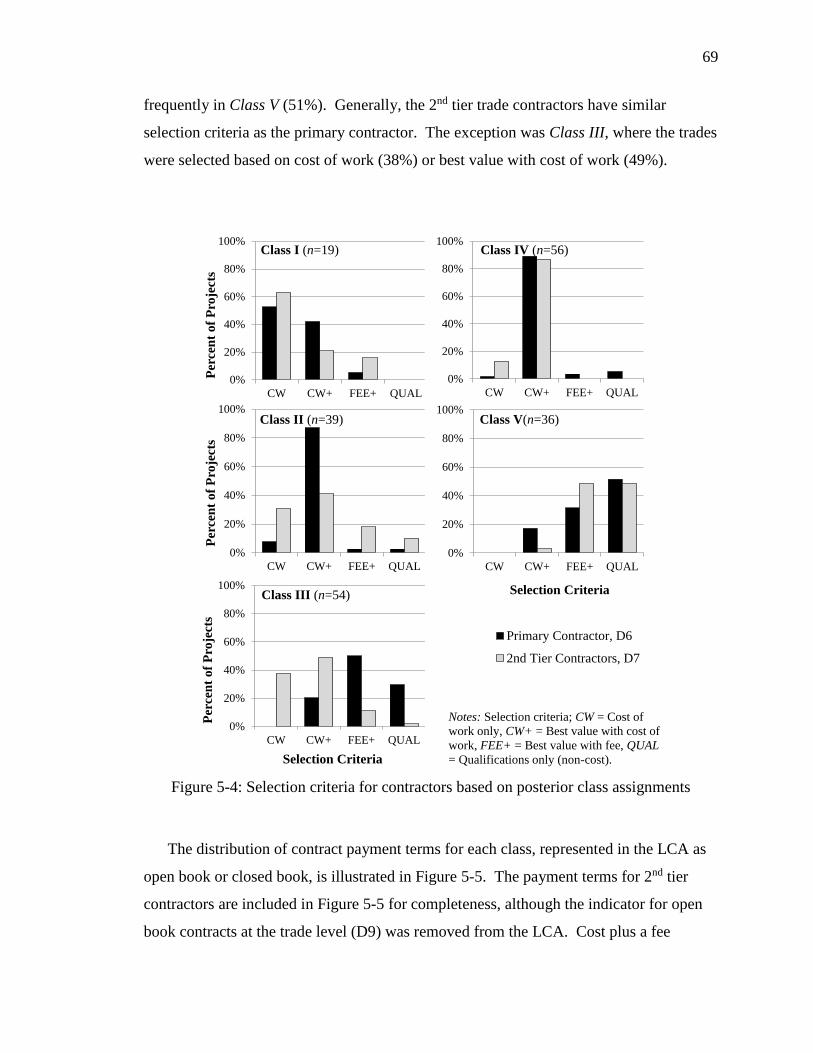
69
frequently in Class V (51%). Generally, the 2nd tier trade contractors have similar
selection criteria as the primary contractor. The exception was Class III, where the trades
were selected based on cost of work (38%) or best value with cost of work (49%).
Figure 5-4: Selection criteria for contractors based on posterior class assignments
The distribution of contract payment terms for each class, represented in the LCA as
open book or closed book, is illustrated in Figure 5-5. The payment terms for 2nd tier
contractors are included in Figure 5-5 for completeness, although the indicator for open
book contracts at the trade level (D9) was removed from the LCA. Cost plus a fee
0%
20%
40%
60%
80%
100%
CW CW+ FEE+ QUAL
Per
cen
t o
f P
roje
cts
Class I (n=19)
0%
20%
40%
60%
80%
100%
CW CW+ FEE+ QUAL
Per
cen
t o
f P
roje
cts
Class II (n=39)
0%
20%
40%
60%
80%
100%
CW CW+ FEE+ QUAL
Per
cen
t o
f P
roje
cts
Selection Criteria
Class III (n=54)
0%
20%
40%
60%
80%
100%
CW CW+ FEE+ QUAL
Class IV (n=56)
0%
20%
40%
60%
80%
100%
CW CW+ FEE+ QUAL
Selection Criteria
Primary Contractor, D6
2nd Tier Contractors, D7
Class V(n=36)
Notes: Selection criteria; CW = Cost of
work only, CW+ = Best value with cost of
work, FEE+ = Best value with fee, QUAL
= Qualifications only (non-cost).

70
payment terms were not common in any class, having a representation of 0% in Class I,
3% in Class II, 13% in Class III, 5% in Class IV and 6% in Class V. Lump sum terms
were most common in Class I (100% of cases in class), Class II (64%) and Class IV
(70%). Conversely, 87% of project in Class II and 64% in Class V had guaranteed
maximum price contract terms for the primary contractor.
Figure 5-5: Payment terms for contractors based on posterior class assignments
0%
20%
40%
60%
80%
100%
LS GMP CPF
Per
cen
t o
f P
roje
cts
0%
20%
40%
60%
80%
100%
LS GMP CPF
Per
cen
t o
f P
roje
cts
0%
20%
40%
60%
80%
100%
LS GMP CPF
Per
cen
t o
f P
roje
cts
Contract Payment Terms
Class III (n=54)
0%
20%
40%
60%
80%
100%
LS GMP CPF
Class IV (n=56)
0%
20%
40%
60%
80%
100%
LS GMP CPF
Contract Payment Terms
Primary Contractor, D8
2nd Tier Contractors, D9
Class V (n=36)
Notes: Payment terms; LS = Lump sum
(Fixed price), GMP = Guaranteed
maximum price, CPF = Cost plus a fee
(Fixed or %).
Class II (n=39)
Class I (n=19)

71
Chapter Summary
The latent class analysis performed for this research revealed five clearly delineated
groups that represent different project delivery strategies used by owners. Although
several indicators were removed from the analysis for not being strong differentiators of
latent class, these indicators may still have a role in project delivery. The latent class
approach recognizes that delivery methods, procurement processes and contractual terms
are not used independently. In practice, common combinations exist to assist owners in
structuring their project organizations. The most common observed variables in each
class were organized in Appendix B. The class assignments made during this analysis
were used to represent project delivery strategies in the structural model.

72
Chapter 6
STRUCTURAL MODELING RESULTS
This chapter uses structural equation modeling to describe the relationships among
team integration, group cohesiveness and performance outcomes, when controlling for
the project delivery strategy, facility size and owner type. A descriptive overview of
projects included in the sample data set is presented. The results of the structural
modeling process are separated into two sections. First, measurement variables for the
latent constructs of team integration and group cohesiveness are validated using factor
analysis techniques. Next, the structural model results for the full project survey data set
are reported. Significant path relationships are discussed relative to primary predictors of
cost, schedule and quality outcomes, and secondary predictors of team integration and
group cohesiveness.
Data Demographics
Of the 204 verified projects in the data set, 62% were publicly funded and 38% were
private. Facilities were classified into one of nine types describing their intended
purpose, including: commercial, lodging, office, correctional, educational,
manufacturing, sports and recreation, transportation and health care. The most
represented facility type was educational, at 27% of the sample, and the least represented
was transportation at only 1%. The prevalence of each facility type, roughly ordered
from low to high complexity and expressed as a percentage of the total sample, is
provided in Figure 6-1. Public owners were most common in educational facilities and
least common in health care.
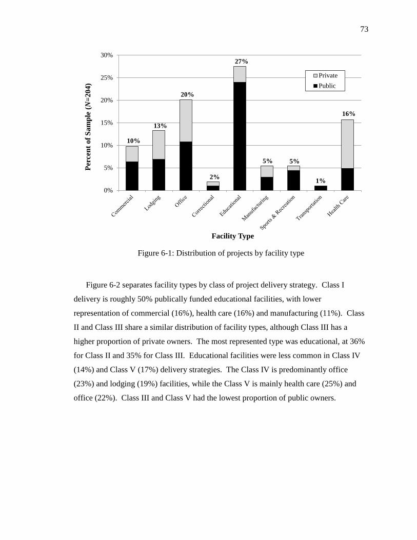
73
Figure 6-1: Distribution of projects by facility type
Figure 6-2 separates facility types by class of project delivery strategy. Class I
delivery is roughly 50% publically funded educational facilities, with lower
representation of commercial (16%), health care (16%) and manufacturing (11%). Class
II and Class III share a similar distribution of facility types, although Class III has a
higher proportion of private owners. The most represented type was educational, at 36%
for Class II and 35% for Class III. Educational facilities were less common in Class IV
(14%) and Class V (17%) delivery strategies. The Class IV is predominantly office
(23%) and lodging (19%) facilities, while the Class V is mainly health care (25%) and
office (22%). Class III and Class V had the lowest proportion of public owners.
0%
5%
10%
15%
20%
25%
30%
Per
cen
t o
f S
am
ple
(N
=2
04
)
Facility Type
Private
Public
10%
13%
20%
16%
2%
27%
5% 5%
1%

74
Figure 6-2: Distribution of facility type by class of project delivery strategy
Projects ranged in size from 5,000 square feet to over 1-million, although
approximately 60% were less than 200,000 square feet. The distribution of facility size
by funding source is shown in Figure 6-3. With the exception of the first and last
0% 10% 20% 30% 40% 50%
Class IV (n=56)14%
23%
19%
14%
4%
11%
4%
2%
9%
0% 10% 20% 30% 40% 50%
Public
Private
Class V (n=36)11%
22%
14%
17%
3%
25%
3%
6%
0% 10% 20% 30% 40% 50%
Commercial
Lodging
Office
Correctional
Educational
Manufacturing
Sports & Recreation
Transportation
Health Care
Class I (n=19)16%
5%
47%
11%
5%
16%
0% 10% 20% 30% 40% 50%
Commercial
Lodging
Office
Correctional
Educational
Manufacturing
Sports & Recreation
Transportation
Health Care
Class II (n=39)8%
18%
15%
36%
6%
13%
3%
3%
0% 10% 20% 30% 40% 50%
Commercial
Lodging
Office
Correctional
Educational
Manufacturing
Sports & Recreation
Transportation
Health Care
Class III (n=54)4%
22%
9%
35%
17%
4%
9%

75
categories, the facility size is grouped in 100,000 square foot increments. The first
category identifies small projects, less than 50,000 square feet, and represents 27% of the
sample. The last category captures the 2% of the sample and represents very large
projects with over 1-million square feet. Compared against the sample proportion of
owner types, public owners were less common on small (55%) and very large projects
(43%) and more common on projects between 150,000 (70%) and 350,000 (71%) square
feet. Since this distribution ranges over several orders of magnitude and is positively
skewed, logarithmic transformations of base 10 were performed prior to structural
modeling.
Figure 6-3: Distribution of project size by square footage
Projects were distributed across the continental United States. As shown in Figure 6-
4, the largest percentages of projects were located Pennsylvania, Colorado and California.
There was strong coverage in the Midwest and South Central regions, but very few
surveys were returned with projects from the North Central states. The sample was
geographically broad and not focused on any single region in the United States.
0%
10%
20%
30%
40%
50%
0 - 99 100 -
199
200 -
299
300 -
399
400 -
499
500 -
599
600 -
699
700 -
799
800 -
899
900 -
999
> 1,000
Per
cen
t o
f S
am
ple
(N
=2
04
)
Facility Size (in 1,000 ft2)
Private
Public
44%
24%
23%
7%
3%1%
3%1% 1% 2%

76
Figure 6-4: Distribution of sample projects across the United States
The unit cost of projects ranged from $50 per square foot to over $1,200, with 55%
reporting less than $400 per square foot. All unit costs were adjusted for time and
location. Using the historical Building Cost Index (BCI) reported monthly by the
Engineering News Record (ENR), all project costs were adjusted for material and labor
price fluctuations between their start of construction and June 2014. Location factors
provided by RSMeans 2014 guidebooks were used to adjust for differences in regional
design and construction costs. Figure 6-5 illustrates the unit cost distribution, with
categories in $100 per square foot increments. Only 3% had unit costs less than $100 per
square foot and were split evenly between public and private ownership. However, the
9% of projects with unit costs exceeding $800 per square foot were predominantly public
(89%). Private funding was most common in projects costing less than $300 per square
foot, but was present in all ranges of unit price. Since unit cost is a function of facility
size and the distribution is similarly positively skewed, unit cost values were transformed
using a base 10 logarithm prior to analysis. Descriptive statistics of the mean, median
and range of each performance measure is provided in Appendix C.
Number of Projects
1 32
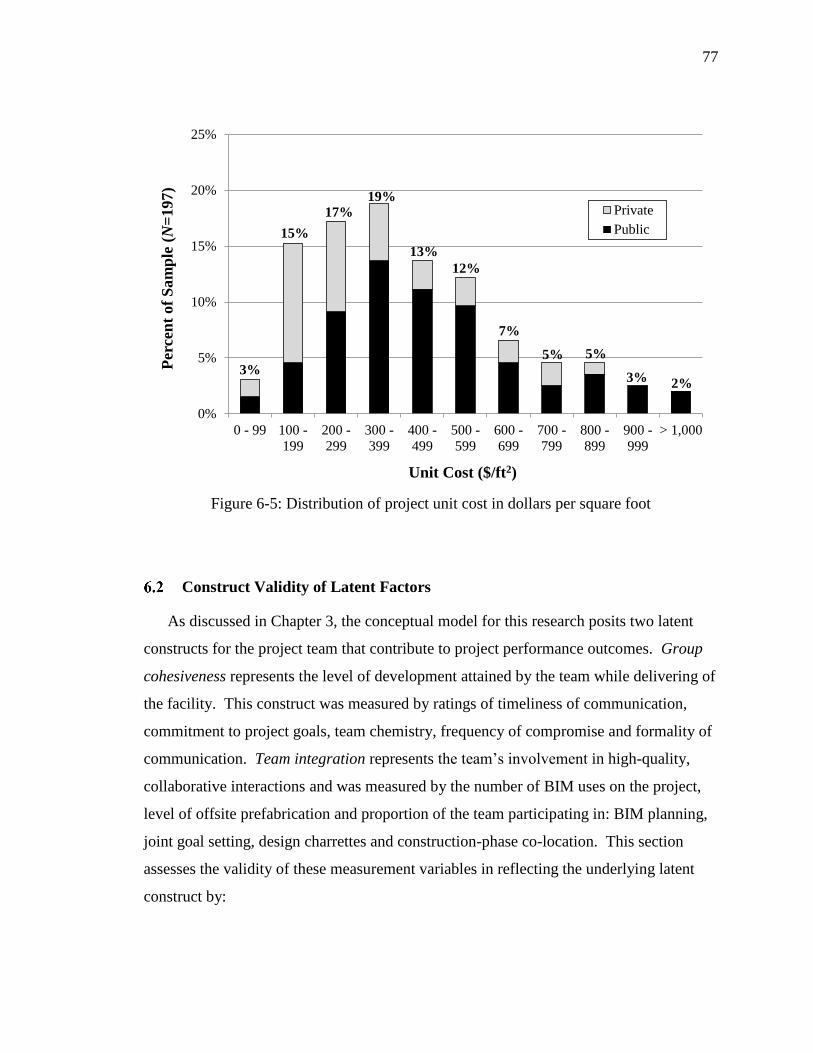
77
Figure 6-5: Distribution of project unit cost in dollars per square foot
Construct Validity of Latent Factors
As discussed in Chapter 3, the conceptual model for this research posits two latent
constructs for the project team that contribute to project performance outcomes. Group
cohesiveness represents the level of development attained by the team while delivering of
the facility. This construct was measured by ratings of timeliness of communication,
commitment to project goals, team chemistry, frequency of compromise and formality of
communication. Team integration represents the team’s involvement in high-quality,
collaborative interactions and was measured by the number of BIM uses on the project,
level of offsite prefabrication and proportion of the team participating in: BIM planning,
joint goal setting, design charrettes and construction-phase co-location. This section
assesses the validity of these measurement variables in reflecting the underlying latent
construct by:
0%
5%
10%
15%
20%
25%
0 - 99 100 -
199
200 -
299
300 -
399
400 -
499
500 -
599
600 -
699
700 -
799
800 -
899
900 -
999
> 1,000
Per
cen
t o
f S
am
ple
(N
=1
97
)
Unit Cost ($/ft2)
Private
Public
3%
15%
17%
19%
13%
12%
7%
5% 5%
3% 2%

78
1) Reviewing a correlation matrix for expected inter-correlations of measurement
variables within each latent construct;
2) Assessing the initial model fit of measurement variables on the theorized 2-factor
model with a confirmatory factor analysis (CFA);
3) Using exploratory factor analysis (EFA) to identify poorly fitting variables that
are not reflective of the desired latent constructs; and
4) Re-visiting the 2-factor CFA with a validated list of measurement variables.
6.2.1 Measurement Variable Correlations
Correlations among variables are of primary interest in factor analysis, which groups
highly inter-correlated variables into fewer number unobserved, latent factors.
Polychoric correlations were calculated to avoid attenuation, since this data consisted of
ordinal rating scales and proportions. Separated by theorized latent constructs, the
correlation matrix for the measurement variables in this study is shown in Table 6-1.
Cohen’s (2013) guidelines are used for interpreting the effect size of correlations. A
correlation coefficient of .10 is a weak or small association, .30 is considered moderate
and greater than .50 is a strong or large correlation. There are strong correlations among
timeliness of commitment (TE1), commitment to project goals (TE2) and team chemistry
(TE3). However, frequency of compromise (TE4) and formality of communication
(TE5) do not appear related with other measures of group cohesiveness. For team
integration, the number of BIM uses (TI2) and participation in BIM planning (TI1), goal
setting (TI3), design charrettes (TI4) and co-location (TI5) are moderately inter-
correlated. The level of offsite prefabrication (TI6) is unrelated to team participation in
design charrettes and co-location. Lastly, there are weak to moderate correlations
between variables across the group cohesiveness and team integration constructs.

79
Table 6-1: Correlation coefficients for team measures
Measure TE1 TE2 TE3 TE5 TE5 TI1 TI2 TI3 TI4 TI5 TI6
Group cohesiveness
TE1. Timeliness of communication 1
TE2. Commitment to project goals .64 1
TE3. Team chemistry .62 .64 1
TE4. Frequency of compromise .25 .12 .23 1
TE5. Formality of communication .09 .03 .02 .01 1
Team integration
TI1. Participation in BIM planning .09 .22 .16 .05 -.04 1
TI2. Number of BIM uses .19 .20 .28 .10 .00 .64 1
TI3. Participation in goal setting .13 .22 .20 .24 -.16 .34 .35 1
TI4. Participation in design charrettes .13 .21 .19 .01 -.13 .23 .35 .30 1
TI5. Participation in co-location .09 .11 .18 .01 -.11 .28 .26 .28 .24 1
TI6. Offsite prefabrication .06 .14 .26 .04 -.05 .26 .22 .14 .13 .15 1
Notes: Polychoric correlations using robust weighted least squares (WLSMV) estimation with
pairwise deletion of missing values; Bolded correlations are significant, p<.05.
6.2.2 Initial Confirmatory Factor Analysis
Confirmatory factor analysis (CFA) tests whether the measurement variables of a
construct or “factor” are consistent with a hypothesized model. In this research, CFA is
used to assess a model that considers variables TE1-TE5 as measures of the group
cohesiveness and TI1-TI6 as measures of the team integration. Two fit indices were
selected to test whether the CFA model represents the data set: the root mean square error
of approximation (RMSEA) and comparative fit index (CFI). RMSEA is a measure of
model misspecification that considers the number of variables in the model. Well-fitting
models have RMSEA less than .08 (Hooper, Coughlan and Muller 2008). The CFI
compares the specified model against a baseline model that assumes no correlation
among observed variables. The resulting index is a value between 0 and 1, with values at
.95 and above indicating a good fit (Hu and Bentler 1999). For this research, the fit
indices for an initial 2-factor confirmatory model exceeded the required levels of fit

80
(CFI=.97, RMSEA=.03), but closer inspection revealed that several variables are not
reflective of the proposed latent constructs. Specifically, low standardized regression
coefficients were found for frequency of compromise (.27), formality of communication
(.01) and offsite prefabrication (.35). When considered alongside similar observations in
the correlation matrix, there is evidence of these three variables having poor association
with their theorized factors.
6.2.3 Exploratory Factor Analysis
Evidence of poor association in a CFA suggests that either (1) some measurement
variables are not reflective of the theorized latent factor, or (2) the variables are better
represented by a different number of underlying factors. Exploratory factor analysis
(EFA) is used to determine the minimum number of latent factors that adequately
describe correlations in a set of measurement variables. Unlike CFA, no preset structure
is imposed that forces variables to group with a specific factor. This EFA was conducted
using robust weighted least squares (WLSMV) estimation and Geomin oblique rotation
for 1-, 2-, and 3-factor solutions. An oblique rotation was selected to allow the extracted
factors to correlate, which is expected in the theoretical model being tested. The 1-factor
solution is a poor fit (CFI=.77, RMSEA=.10) and the 3-factor solution offers only a small
improvement (ΔCFI=.01, ΔRMSEA=.03) over the 2-factor at the cost of added model
complexity. This comparison confirms that the set of measurement variables (TE1-TE5,
TI1-TI6) are adequately represented by a 2-factor latent model.
The 2-factor EFA solution identifies three poorly fitting variables across both latent
constructs. For a sample size of 200, variables should achieve a rotated loading of at
least .40 to be considered reflective of the underlying factor (Stevens 2012). As shown in
Table 6-2, the frequency of compromise (TE5) and level offsite prefabrication (TI6) have
rotated loadings below .30 on Factor #1 and Factor #2, respectively. Formality of
communication (TE5) has weak loadings across both factors, at .14 on Factor #1 and -.20
on Factor #2. Therefore, these three measurement variables do not appear to reflect the

81
same latent factors as TE1-TE3 and TI1-TI5, and should be removed to improve the
validity of the constructs.
Table 6-2: Rotated loadings for 2-factor EFA of team measures
Factor
Theorized Factor Components 1 2
Group cohesiveness TE1. Timeliness of communication .87 -.16
TE2. Commitment to project goals .80 .01
TE3. Team chemistry .77 .05
TE4. Frequency of compromise .24 .05
TE5. Formality of communication .14 -.20
Team integration TI1. Participation in BIM planning -.07 .67
TI2. Number of BIM uses .02 .66
TI3. Participation in goal setting .01 .58
TI4. Participation in design charrettes .02 .47
TI5. Participation in co-location -.05 .47
TI6. Offsite prefabrication .06 .29
Notes: Goodness-of-fit summary: CFI=.98, RMSEA=.04; EFA with robust
weighted least squares (WLSMV) estimation and oblique rotation.
Loadings greater than .40 are highlighted to aid in interpretation.
6.2.4 Poorly Fitting Measurement Variables
Poorly fitting variables in a factor analysis are unreliable in providing information
about the underlying latent construct. However, removing the variables for frequency of
compromise (TE4), formality of communication (TE5) and offsite prefabrication (TI6)
from their respective latent constructs does not suggest that theories supporting the
inclusion of these variables are invalid. Compromise and formality of interactions have
reasonable, theoretical justification in literature for being considered a product of the
group cohesiveness. Likewise, offsite prefabrication and modularization of building
systems often benefit from more integrated teams.

82
In this research, the lack of measurement reliability in TE4, TE5 and TI6 was likely
the result of unclear survey questions. For example, respondent ratings to the question
“How often did the project team compromise on project issues?” are biased by whether
they perceive compromise as a positive or negative influence. Taking a positive
perspective, compromise allows the team to move forward with design options or
construction plans that strike a balance between the competing interests of each
participant. Alternately, compromise may be viewed negatively, as a sub-optimal
solution where no one is satisfied and the project suffers as a result. Since no definition
of comprise was provided with the survey, both perspectives are represented in the data
set, leading to inconsistent measurements. A similar susceptibility to respondent bias can
be observed in evaluating communication formality. Without a strict definition for
“formal” and “informal”, the question lacked objectivity and was too open to respondent
interpretation. Lastly, responses from owners may lack the perspective to provide an
accurate assessment on the level of offsite prefabrication on their project. Unless the
specification explicitly calls for prefabricated or modularized systems, the decision to use
offsite resources often lies with the primary contractor and specialty trades. Therefore,
the question regarding offsite prefabrication was likely inappropriate for owners as the
targeted survey response group.
6.2.5 Revised Confirmatory Factor Analysis
After removing poorly fitting variables, a second CFA was conducted to verify the
final factor structure. Illustrated in Figure 6-6, with both standardized and
unstandardized coefficients, the 2-factor model of group cohesiveness and team
integration is well representative of the data (CFI=1.0, RMSEA=.00). The large
standardized regression coefficients on the measurement variables for group cohesiveness
construct indicate that team chemistry (.80), timeliness of communication (.76) and goal
commitment (.83) are reflective of the same underlying latent variable. Similarly, the
CFA produced moderate to large coefficients for variables measuring team integration,
including the number of BIM uses (.72), participation in BIM planning (.61), goal setting

83
(.57), design charrettes (.50) and co-location (.43). Lastly, as expected from the
theoretical model, the latent constructs are positively correlated.
Figure 6-6: Revised CFA with unstandardized (A) and standardized (B) estimates
Factoring Performance Outcomes
Although not explicitly theorized, the correlations among performance outcomes
were examined for the presence of underlying latent factors. A correlation matrix for
cost and schedule metrics, as well as facility quality ratings is provided in Table 6-3.
Since these measures are a combination of continuous and ordinal data, polychoric
correlation coefficients were calculated and interpreted similarly to previous discussions
of correlation. There are strong correlations between unit cost and intensity (.59), and
between delivery speed and construction speed (.95). Both relationships are expected,
since intensity is a function of unit cost and the construction duration is a subset of the
project duration. While each pair of correlated metrics could be reduced to a single
ChemistryComm.
Timeliness
Goal
Commit.
BIM UsesBIM Plan
Partic.
Charrette
Partic.
Colocation
Partic.
R2=.64 R2=.58 R2=.68
R2=.51 R2=.34 R2=.25 R2=.18
.80.76
.83
.72 .43.61 .50
Group
Cohesiveness
Team
Integration
Goal Set
Partic.
R2=.32
.57
.39
ChemistryComm.
Timeliness
Goal
Commit.
BIM UsesBIM Plan
Partic.
Charrette
Partic.
Colocation
Partic.
R2=.64 R2=.58 R2=.68
R2=.51 R2=.34 R2=.25 R2=.18
.97.93
1
1 .13.18 .14
Group
Cohesiveness
Team
Integration
Goal Set
Partic.
R2=.32
.10
.34
A. B.
Notes: Goodness-of-fit summary: χ2(204)/df=16.6, p=.62, CFI=1.0, RMSEA=.00

84
factor, there is little improvement to model interpretability when introducing additional
factors with only two measurement variables. However, the pattern of correlations
among quality ratings suggests the influence of one or more latent factors. The moderate
to strong inter-correlations among ratings for difficulty of start-up, magnitude of call
backs and operation costs (.48 to .68) seem to reflect the owner’s turnover experience.
And the large correlations among ratings for the quality of structure and envelope,
interior finishes and environmental systems (.56 to .62) are indicative of the facility’s
system quality.
Table 6-3: Correlation coefficients for project performance variables
Measure 1 2 3 4 5 6 7 8 9 10 11 12
Project performance
1. Unit cost (Log) 1
2. Intensity (Log) .59 1
3. Project cost growth .03 -.13 1
4. Delivery speed (Log) -.26 -.14 -.06 1
5. Construction speed (Log) -.26 -.28 -.04 .95 1
6. Project schedule growth .09 -.15 .19 -.16 -.15 1
Facility quality
7. Difficulty of start-up -.27 -.07 -.24 .02 -.03 -.11 1
8. Magnitude of call backs -.22 -.02 -.29 .05 .01 -.21 .68 1
9. Operation costs -.16 -.10 -.21 -.01 -.05 -.11 .48 .60 1
10. Structure and envelope .04 -.11 -.14 .26 .27 -.08 .17 .17 .26 1
11. Interior finishes .15 -.17 .12 .13 .17 .04 .02 .08 .26 .58 1
12. Environmental systems .04 -.09 -.14 .17 .18 -.13 .13 .34 .38 .62 .56 1
Notes: Polychoric correlations using robust weighted least squares (WLSMV) estimation with
pairwise deletion of missing values; Bolded coefficients are significant, p<.05
An EFA was performed on the six quality measures to determine if the inter-
correlations may be explained by one or more latent factors. The 1-factor model was a
very poor fit (CFI=.78, RMSEA=.31), but the 2-factor solution was adequate (CFI=.99,
RMSEA=.07). Shown in Table 6-4, difficulty of start-up (Q1), magnitude of call backs
(Q2) and operation costs (Q3) have rotated loadings of .60 or greater in Factor #1 and the
quality of structure and envelope (Q4), interior finishes (Q5) and environmental systems
(Q6) have rotated loadings on .75 of greater in Factor #2. This is reasonable evidence to

85
support the use of two continuous latent factors, turnover experience and facility quality,
as representative of quality performance outcomes.
Table 6-4: Rotated loadings for 2-factor EFA of quality ratings
Factor
Theorized Factor Components 1 2
Turnover experience Q1. Difficulty of start-up .76 -.06
Q2. Magnitude of call backs .92 .00
Q3. Operation costs .60 .23
Facility quality Q4. Structure and envelope .00 .78
Q5. Interior finishes -.11 .77
Q6. Environmental systems .12 .75
Notes: Goodness-of-fit summary: CFI=.99, RMSEA=.07; EFA with robust
weighted least squares (WLSMV) estimation and oblique rotation.
Loadings greater than .40 are highlighted to aid in interpretation.
Specifying the Structural Model
Due to the flexibility of structural model specification, a variety of models can be
conceived. As discussed in Chapter 4, the framework for this research contained three
focal blocks: (1) the project delivery strategy, (2) the quality of inter-organizational
relationships, as represented by constructs of team integration and group cohesiveness,
and (3) the project’s performance. Programming factors, including owner type and
facility size, were seen as control variables. Several structural models, assembled from
two or more of these focal blocks, were explored for both model fit and predictive
capability. The specification of these model alternatives is shown in Figure 6-7.
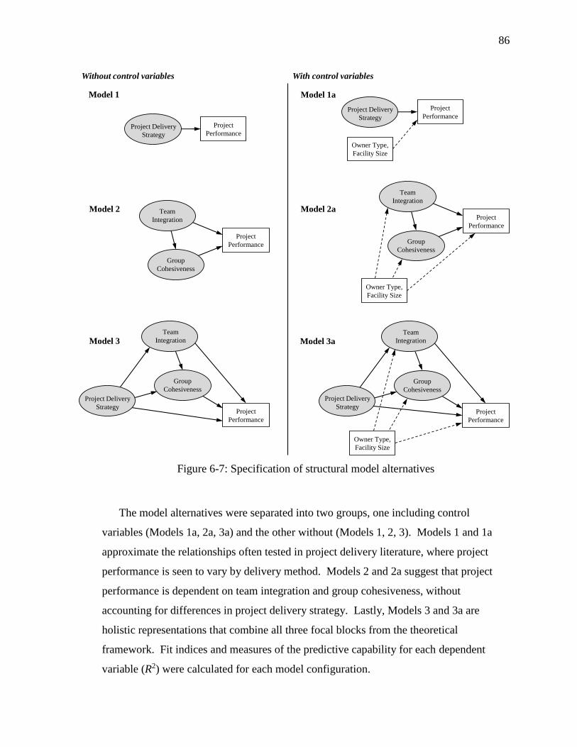
86
Figure 6-7: Specification of structural model alternatives
The model alternatives were separated into two groups, one including control
variables (Models 1a, 2a, 3a) and the other without (Models 1, 2, 3). Models 1 and 1a
approximate the relationships often tested in project delivery literature, where project
performance is seen to vary by delivery method. Models 2 and 2a suggest that project
performance is dependent on team integration and group cohesiveness, without
accounting for differences in project delivery strategy. Lastly, Models 3 and 3a are
holistic representations that combine all three focal blocks from the theoretical
framework. Fit indices and measures of the predictive capability for each dependent
variable (R2) were calculated for each model configuration.
Project
PerformanceProject Delivery
Strategy
Project
Performance
Team
Integration
Group
Cohesiveness
Project
Performance
Team
Integration
Group
Cohesiveness
Project Delivery
Strategy
Project
PerformanceProject Delivery
Strategy
Owner Type,
Facility Size
Project
Performance
Team
Integration
Group
Cohesiveness
Owner Type,
Facility Size
Project
Performance
Team
Integration
Group
Cohesiveness
Project Delivery
Strategy
Owner Type,
Facility Size
Model 1
Model 2
Model 3
Model 1a
Model 2a
Model 3a
Without control variables With control variables

87
The goodness-of-fit indices for these model alternatives are provided in Table 6-5.
All model alternatives achieved the minimum fit criteria for this study. Model 2 was the
overall best fit (CFI=.99, RMSEA=.01), and Models 1 (CFI=.96, RMSEA=.05) and 1a
(CFI=.97, RMSEA=.06) were comparatively the weakest. Model 3a, with the most
variables and path relationships, was in the middle of the range for fit indices (CFI=.99,
RMSEA=.03). The addition of control variables improved the CFI for all models. The
RMSEA, which favors parsimony and fewer estimated parameters in the model, was
slightly worsened with addition of control variables. These goodness-of-fit indices
reflect the specified model’s ability account for the sample covariance. However,
structural models may have a strong fit to the data without having much predictive
capability on the dependent variables.
Table 6-5: Fit indices of structural model alternatives
Fit Indices
Model Specification χ2 df CFI RMSEA
Models without control variables
Model 1: Project delivery strategy 68.6 48 .96 .05
Model 2: Team integration, group cohesiveness 134.2 131 .99 .01
Model 3: Project delivery strategy, team integration, group
cohesiveness
180.4 171 .99 .02
Models with control variables
Model 1a: Project delivery strategy, controls 96.4 56 .97 .06
Model 2a: Team integration, group cohesiveness, controls 164.5 151 .99 .02
Model 3a: Project delivery strategy, team integration, group
cohesiveness, controls
218.2 191 .99 .03
For each model alternative, the percent of variance explained for each dependent
variable (R2) is summarized in Table 6-6. Although Model 2 had the best overall fit, its
usefulness as a predictor of project performance was very low, explaining only 6% of the
variance in cost growth and 5% in schedule growth. The addition of control variables

88
into the model greatly improved the prediction of delivery and construction speeds,
improving their respective R2 from 8% to 84% in the most extreme case. Team
integration and group cohesiveness were most influential in predicting cost growth,
schedule growth, system quality and turnover experience. Model 3a consistently
explained a larger percent of variance than the alternative models, and when considered
alongside strong fit indices, was the model specification used in this research.
Table 6-6: Predictive capability of structural model alternatives
Predictive Capability (R2)
Without control variables With control variables
Model Variable Model 1 Model 2 Model 3 Model 1a Model 2a Model 3a
Team integration -- -- .28 -- .16 .46
Group cohesiveness -- .15 .19 -- .15 .20
Project cost growth .03 .06 .09 .05 .08 .11
Unit cost .02 .07 .15 .12 .20 .25
Intensity .09 .05 .11 .26 .33 .25
Project schedule growth .01 .05 .08 .04 .08 .14
Delivery speed .13 .19 .20 .84 .79 .84
Construction speed .08 .14 .15 .84 .83 .84
System quality .12 .42 .53 .21 .44 .51
Turnover experience .07 .26 .29 .12 .35 .38
Primary Structural Model Results
The presentation and discussion of structural model results is separated into two
sections. First, primary results will examine predictors of cost, schedule and quality
performance within the context of the structural model. Then, secondary results will
consider the predictors of team integration and group cohesiveness as intermediate
outcomes. The structural model was calculated using MPlus Version 7.2 statistical
software with robust weighted least square (WLSMV) estimation of regression paths.
The discrete classes of project delivery strategies from Chapter 5 were split into five
dummy coded variables, with Class I delivery serving as the baseline for comparison.

89
Logarithmic transformations were used for variables that were a function of the gross
square-footage of the facility, such as unit cost or delivery speed. These variables tended
to have non-constant variance that increased with facility size. Prior to interpreting the
results of transformed regression coefficients, the coefficients were back-transformed as
the percent change in a dependent variable, given a one unit change in the independent
variable.
The calculated structural model diagram is presented in Figure 6-8, with
unstandardized coefficients, and Figure 6-9, with standardized values. For simplicity,
only significant paths are shown in these diagrams (p<.05) and the classes of project
delivery strategy are represented by a single categorical latent variable. For primary or
secondary outcomes that varied by project delivery strategy, path coefficients and
significance tests are provided in the table below the model diagram. All latent
constructs and outcome variables were controlled for by owner type and facility size. A
complete diagram of the structural model that includes insignificant paths, control
variable paths and dummy coded variables is provided in Appendix D. All discussion of
model results will use the unstandardized coefficients from Figure 6-8 to facilitate direct
interpretation.
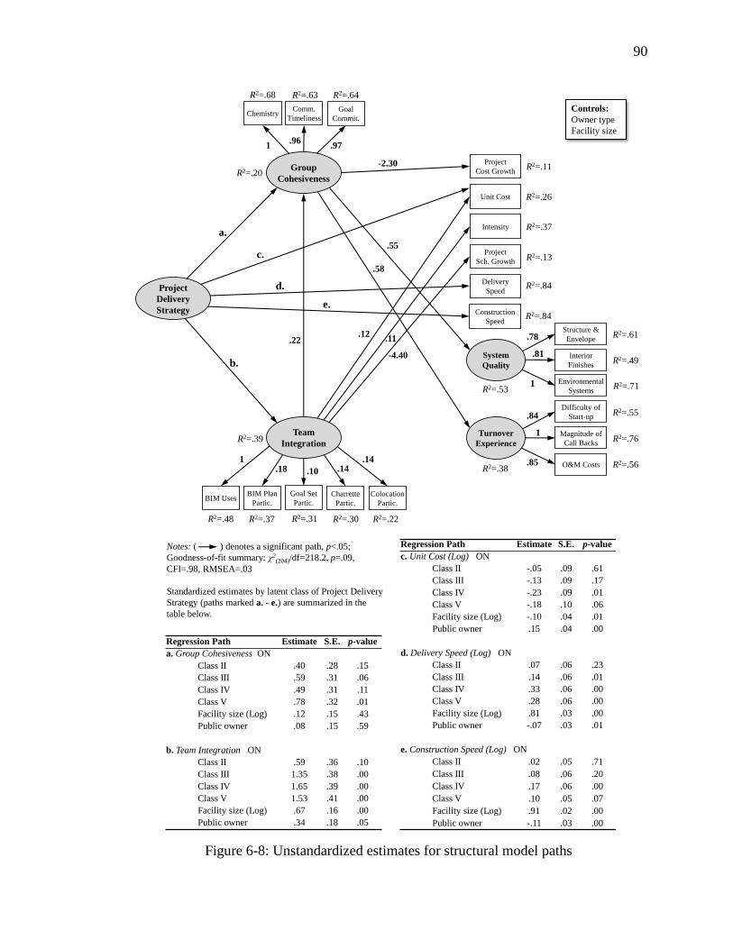
90
Figure 6-8: Unstandardized estimates for structural model paths
Project
Cost Growth
Project
Sch. Growth
Delivery
Speed
Unit Cost
Difficulty of
Start-up
Magnitude of
Call Backs
O&M Costs
Structure &
Envelope
Interior
Finishes
Environmental
Systems
System
Quality
Turnover
Experience
ChemistryComm.
Timeliness
Goal
Commit.
R2=.68 R2=.63 R2=.64
R2=.39
R2=.20R2=.11
R2=.26
R2=.13
R2=.84
R2=.61
R2=.49
R2=.71
R2=.55
R2=.76
R2=.56R2=.38
R2=.53
c.
d.
Intensity R2=.37
Construction
SpeedR2=.84
Project
Delivery
Strategy
Group
Cohesiveness
e.
b.
BIM UsesBIM Plan
Partic.
Charrette
Partic.
Colocation
Partic.
R2=.48 R2=.37 R2=.30 R2=.22
Team
Integration
Goal Set
Partic.
R2=.31
a.
Controls:
Owner type
Facility size
.22
-2.30
.58
.55
.12
-4.40
1.96
.97
.11
1 .14.18 .14.10
.78
.81
1
.84
1
.85
Regression Path Estimate S.E. p-value
a. Group Cohesiveness ON
Class II .40 .28 .15
Class III .59 .31 .06
Class IV .49 .31 .11
Class V .78 .32 .01
Facility size (Log) .12 .15 .43
Public owner .08 .15 .59
b. Team Integration ON
Class II .59 .36 .10
Class III 1.35 .38 .00
Class IV 1.65 .39 .00
Class V 1.53 .41 .00
Facility size (Log) .67 .16 .00
Public owner .34 .18 .05
Regression Path Estimate S.E. p-value
c. Unit Cost (Log) ON
Class II -.05 .09 .61
Class III -.13 .09 .17
Class IV -.23 .09 .01
Class V -.18 .10 .06
Facility size (Log) -.10 .04 .01
Public owner .15 .04 .00
d. Delivery Speed (Log) ON
Class II .07 .06 .23
Class III .14 .06 .01
Class IV .33 .06 .00
Class V .28 .06 .00
Facility size (Log) .81 .03 .00
Public owner -.07 .03 .01
e. Construction Speed (Log) ON
Class II .02 .05 .71
Class III .08 .06 .20
Class IV .17 .06 .00
Class V .10 .05 .07
Facility size (Log) .91 .02 .00
Public owner -.11 .03 .00
Notes: ( ) denotes a significant path, p<.05;
Goodness-of-fit summary: χ2(204)/df=218.2, p=.09,
CFI=.98, RMSEA=.03
Standardized estimates by latent class of Project Delivery
Strategy (paths marked a. - e.) are summarized in the
table below.
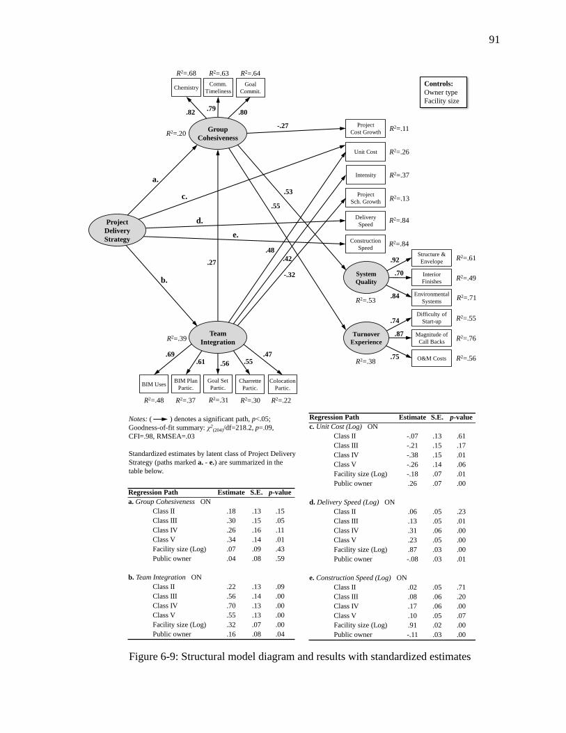
91
Figure 6-9: Structural model diagram and results with standardized estimates
Project
Cost Growth
Project
Sch. Growth
Delivery
Speed
Unit Cost
Difficulty of
Start-up
Magnitude of
Call Backs
O&M Costs
Structure &
Envelope
Interior
Finishes
Environmental
Systems
System
Quality
Turnover
Experience
ChemistryComm.
Timeliness
Goal
Commit.
R2=.68 R2=.63 R2=.64
R2=.39
R2=.20R2=.11
R2=.26
R2=.13
R2=.84
R2=.61
R2=.49
R2=.71
R2=.55
R2=.76
R2=.56R2=.38
R2=.53
.27
-.27
.55
.53
.48
-.32
c.
d.
Intensity R2=.37
Construction
SpeedR2=.84
.82.79
.80
Project
Delivery
Strategy
Group
Cohesiveness
e.
.42
b.
BIM UsesBIM Plan
Partic.
Charrette
Partic.
Colocation
Partic.
R2=.48 R2=.37 R2=.30 R2=.22
.69 .47.61 .55
Team
Integration
Goal Set
Partic.
R2=.31
.56
a.
.92
.70
.84
.74
.87
.75
Controls:
Owner type
Facility size
Regression Path Estimate S.E. p-value
a. Group Cohesiveness ON
Class II .18 .13 .15
Class III .30 .15 .05
Class IV .26 .16 .11
Class V .34 .14 .01
Facility size (Log) .07 .09 .43
Public owner .04 .08 .59
b. Team Integration ON
Class II .22 .13 .09
Class III .56 .14 .00
Class IV .70 .13 .00
Class V .55 .13 .00
Facility size (Log) .32 .07 .00
Public owner .16 .08 .04
Regression Path Estimate S.E. p-value
c. Unit Cost (Log) ON
Class II -.07 .13 .61
Class III -.21 .15 .17
Class IV -.38 .15 .01
Class V -.26 .14 .06
Facility size (Log) -.18 .07 .01
Public owner .26 .07 .00
d. Delivery Speed (Log) ON
Class II .06 .05 .23
Class III .13 .05 .01
Class IV .31 .06 .00
Class V .23 .05 .00
Facility size (Log) .87 .03 .00
Public owner -.08 .03 .01
e. Construction Speed (Log) ON
Class II .02 .05 .71
Class III .08 .06 .20
Class IV .17 .06 .00
Class V .10 .05 .07
Facility size (Log) .91 .02 .00
Public owner -.11 .03 .00
Notes: ( ) denotes a significant path, p<.05;
Goodness-of-fit summary: χ2(204)/df=218.2, p=.09,
CFI=.98, RMSEA=.03
Standardized estimates by latent class of Project Delivery
Strategy (paths marked a. - e.) are summarized in the
table below.

92
6.5.1 Cost Performance
Cost performance was measured using three metrics: project cost growth, unit cost
and intensity. These metrics were treated as separate dependent variables in the structural
model and regressed on the latent constructs of project delivery strategy, team integration
and group cohesiveness. The owner type and facility size were included in the model to
control for funding source and project scale, respectively. In this manner, the significant
effects of the latent constructs on cost performance were separated from the effects of
other explanatory variables. A p-value of .05 was selected as the cut-off for determining
statistical significance.
Project cost growth was defined as the percent difference between the actual and
planned costs of design and construction services. Group cohesiveness was the only
significant predictor of project cost growth (p=.00), when controlling for project delivery
strategy, team integration, owner type and facility size. Improving the group
cohesiveness by one unit, reduced the mean cost growth by 2.3%; although the overall
variation explained was low (R2=.11). In the context of this model, there was no
significant difference in mean cost growth across the discrete classes of project delivery
strategy (.36 ≤ p ≤ .93) and no significant linear relationship between cost growth and
team integration (p=.79, owner type (p=.11) or facility size (p=.41).
Unit cost, or cost per square foot, was calculated as the actual design and construction
costs divided by the gross square footage of the facility. The unit cost was adjusted for
time and location using historical indices, and transformed using a base 10 logarithm.
Both project delivery strategy and team integration were significant predictors of unit
cost (p=.01), when controlling for group cohesiveness, owner type and facility size.
These relationships explained a total of 26% of the variation in unit cost. The Class IV
was the only project delivery strategy that showed significantly different unit costs when
compared against Class I delivery, averaging 41% cheaper (p=.01) after accounting for
differences in group cohesiveness, team integration, owner type and gross square footage
of the facility. The Class V averaged 34% cheaper than Class I delivery, at a nearly
significant level (p=.06). Within the context of this model, an increase of one unit in

93
team integration was found to increase unit cost by 32% (p=.00), having a public owner
resulted in 39% higher mean unit cost (p=.00) and increasing the facility size by 10%
reduced the unit cost by approximately 1% (p=.01). There was no significant linear
relationship between group cohesiveness and unit cost (p=.27).
Intensity was defined as the cost per square foot installed per month of project
duration, using the actual design and construction costs and the duration from start of
design until substantial completion. Intensity values were adjusted for time and location
using historical indices, and transformed using a base 10 logarithm. Team integration
was the only significant predictor of intensity (p=.00), when controlling for project
delivery strategy, group cohesiveness, owner type and facility size. An increase of one
unit in team integration resulted in 29% higher intensity (p=.00). Increasing the facility
size by 10% reduced the overall intensity by 2.8% (p=.00) and having a public owner
increased intensity by 20% (p=.03), explaining a moderate amount of variation (R2=.37).
There was no significant difference in mean intensity across the classes of project
delivery strategy (.27 ≤ p ≤ .86) and no significant linear relationship between group
cohesiveness and intensity (p=.16).
6.5.2 Schedule Performance
Schedule performance was measured with three metrics: project schedule growth,
delivery speed and construction speed. These metrics were treated as separate dependent
variables in the structural model and regressed on the latent constructs of project delivery
strategy, team integration and group cohesiveness. The owner type, either public of
private, and facility size, as the gross square foot area, were included in the model to
control for funding source and project scale, respectively.
Project schedule growth was calculated as the percent difference between the planned
and actual project duration, measured from the start of design to substantial completion.
Team integration was the only significant predictor of schedule growth (p=.01), when
controlling for project delivery strategy, group cohesiveness, owner type and facility size.

94
Public owners experienced a 7% higher mean schedule growth, at a nearly significant
level (p=.06). An increase of one unit in team integration reduced the mean schedule
growth by 4.4%; although the overall variation explained was low (R2=.13). There was
no significant difference in mean schedule growth across the classes of project delivery
strategy (.07 ≤ p ≤ .53), and no significant linear relationship between group cohesiveness
and schedule growth (p=.10) or between facility size and schedule growth (p=.37).
Delivery speed was defined as the gross square foot area of the facility divided by the
actual project duration in months, from start of design to substantial completion. Similar
to other metrics calculated using facility size, he delivery speed values were transformed
using a base 10 logarithm. Project delivery strategy, owner type and facility size were
significant predictors of delivery speed, when controlling for group cohesiveness and
team integration. Within the classes of project delivery strategy, there was no significant
difference in mean delivery speed between Class II and Class I delivery (p=.23).
However, when compared against Class I delivery, the mean delivery speed for Class III
was 38% faster (p=.01), Class IV was 111% faster (p=.00) and Class V was 91% faster
(p=.00). Within the context of this model, having a public owner resulted in a 15%
slower delivery speed (p=.01) and increasing the facility size by 10% increased the
delivery speed by 8% (p=.00). Approximately 86% of the variation in delivery speed was
accounted for in this model. There was no significant linear relationship between group
cohesiveness and delivery speed (p=.97) or team integration and delivery speed (p=.53).
Construction speed was defined as the gross square footage of the facility divided by
the actual construction duration, from groundbreaking to substantial completion. The
construction speeds were transformed using a base 10 logarithm for analysis. Project
delivery strategy, owner type and facility size were significant predictors of construction
speed, when controlling for group cohesiveness and team integration; explaining a large
portion of the variation in construction speed (R2=.84). Within the classes of project
delivery strategy, there was no significant difference in mean construction speed between
Class II (p=.71) or Class III (p=.20) and Class I delivery. The Class IV was 45% faster
during construction (p=.00), when compared against Class I delivery. Although not quite
95
significant, the Class V had a 27% higher mean construction speed (p=.07) than Class I
delivery. Within the context of the model, having a public owner resulted in 25% slower
construction speed (p=.00) and increasing the facility size by 10% increased the
construction speed by 7.5% (p=.00). There was no significant relationship between
group cohesiveness and construction speed (p=.99) or team integration and construction
speed (p=.25).
6.5.3 Quality Performance
Quality performance was represented by two latent constructs: turnover experience
and overall facility quality. These latent constructs were treated as separate dependent
variables in the structural model and regressed on the other latent constructs of project
delivery strategy, team integration and group cohesiveness. The owner type, either
public of private, and facility size, as the gross square foot area, were included in the
model to control for funding source and project scale, respectively.
Turnover experience was measured by the owner’s rating for difficulty of start-up,
magnitude of call backs and operation and maintenance (O&M) costs. The rating scales
were oriented such that higher scores of turnover experience signify easier start-up, fewer
call backs and lower O&M costs. Group cohesiveness and facility size were significant
predictors of turnover experience, when controlling for project delivery strategy, team
integration and owner type. For a one unit increase in group cohesiveness, the turnover
experience was improved by .58 units (p=.00). For projects with public owners, the mean
turnover experience was .55 units less than private owners (p=.00). This model explains
38% of the variation in the turnover experience construct. There was no significant
difference in turnover experience across the classes of project delivery strategy (.16 ≤ p ≤
.99) and no significant linear relationship between team integration and turnover
experience (p=.54) or facility size and turnover experience (p=.30).
Overall facility quality was measured by the owner’s rating of satisfaction with the
structure and building envelope, interior finishes and environmental systems. The rating

96
scales were oriented such that higher levels of overall facility quality signify greater
satisfaction with the structure and envelope, interior finishes and environmental systems.
Group cohesiveness was the only significant predictor of overall facility quality, when
controlling for project delivery strategy, team integration, owner type and facility size.
When group cohesiveness increases by one unit, the mean facility quality increases by
.55 units (p=.00); explaining a moderate amount of variation (R2=.53). Although not
quite significant, an increase in one unit of team integration improved facility quality by
.22 units (p=.06). There was no significant difference in facility quality across the classes
of project delivery strategy (.13 ≤ p ≤ .78) or with owner type (p= .51) and facility size
(p=.15).
6.5.4 Summary of Primary Results
Structural modeling provided a robust method of examining the simultaneous
influence of group cohesiveness and team integration on project performance, within the
context of a project delivery strategy, funding source and facility size. Facility type was
not accounted for in the model. Table 6-7 provides a high level summary of significant
linear relationships between predictors and outcomes. The directionality of each
association is listed as either positive or negative. There were measurable differences in
unit cost, delivery speed and construction speed across classes of project delivery
strategy, when compared against Class I delivery. Team integration was a contributor to
unit cost, intensity and schedule growth, while the group cohesiveness helped to predict
cost growth, turnover experience and facility quality. Projects with higher team
integration scores used BIM in design and coordination applications, and involved more
of the team in BIM planning, goal setting, design charrettes and construction-phase co-
location. Higher group cohesiveness scores resulted in better team chemistry, stronger
commitment to project goals and more on-time communication.

97
Tab
le 6
-7:
Sum
mar
y o
f p
rim
ary o
utc
om
e re
lati
onsh
ips
from
str
uct
ura
l m
od
el
Qu
ali
ty
Turn
ove
r
exper
ien
ce
(–) +
38%
Note
s: 1
Pro
ject
del
iver
y s
trat
egie
s co
mpar
ed a
gai
nst
Cla
ss I
; (+
) S
ignif
ican
t posi
tive
rela
tionsh
ip b
etw
een p
redic
tor
and
outc
om
e, p
<.0
5;
(–)
Sig
nif
ican
t neg
ativ
e re
lati
onsh
ip.
p<
.05.
Faci
lity
quali
ty
+
53%
Sch
edu
le
Sch
edule
gro
wth
+
(–)
13%
Del
iver
y
spee
d
+
+
+
(–)
+
84%
Const
ruct
ion
spee
d
+
(–)
+
84%
Cost
Cost
gro
wth
(–)
11%
Unit
cost
(–) +
(–)
+
26%
Inte
nsi
ty
+
37%
Pre
dic
tor
Cla
ss I
I1
Cla
ss I
II1
Cla
ss I
V1
Cla
ss V
1
Publi
c ow
ner
Fac
ilit
y s
ize
Tea
m i
nte
gra
tion
Gro
up c
ohes
iven
ess
Vari
an
ce e
xp
lain
ed:

98
Secondary Structural Model Results
Whereas the discussion of primary results focused on predictors of cost, schedule and
quality outcomes, this section reviews predictors of team integration and group
cohesiveness as intermediate or secondary outcomes in the structural model. When
primary outcomes are dependent on these latent team constructs, the model paths
discussed in this section identify the explanatory variables that influence team integration
and group cohesiveness.
6.6.1 Team Integration
The team integration construct was measured by the number of BIM uses selected by
the respondent from a prescribed list and the proportion of the team participating in: BIM
planning, goal setting, design charrettes and construction-phase co-location. The rating
scales were oriented such that higher scores of team integration were reflective of a
higher number BIM uses and greater proportions of team participation in collaborative
interactions. In creating the proportions, a full team consisted of at least one
representative from each of the five main players on the project: owner, designer, primary
contractor, MEP trade contractor and structural trade contractor. Project delivery
strategy, owner type and facility size were all significant predictors of team integration.
Within the classes of project delivery strategy, there was no significant difference in
mean team integration between Class II (p=.10) and Class I delivery. In order of
increasing means of team integration, Class III (1.35), Class V (1.53) and Class IV (1.65)
were all significantly different from Class I delivery (p=.00). Within the context of this
model, having a public owner increased the mean team integration by .34 (p=.05) and a
10% increase in facility size increases team integration by .07 units (p=.00).
6.6.2 Group Cohesiveness
The group cohesiveness construct was measured by ratings of goal commitment, team
chemistry and timeliness of communication. The rating scales were oriented such that
higher scores of group cohesiveness were associated with stronger goal commitment,
99
better team chemistry and more frequent on-time communication. The ratings were self-
reported by the respondent and reflect their perception of the group cohesiveness after the
completion of the project. Project delivery strategy and team integration were both
significant predictors of group cohesiveness, when controlling for owner type and facility
size. Within the classes of project delivery strategy, there was no significant difference in
mean group cohesiveness between Class II (p=.15) or Class IV (p=.11) and Class I
delivery. The Class V had a higher mean group cohesiveness score (p=.01), when
compared against Class I delivery. Although not quite significant, Class III was also
associated with a better group cohesiveness (p=.06) than Class I delivery. For an increase
of one unit in team integration, the group cohesiveness improved by .22 units (p=.03).
This model explained 20% of the variation in the group cohesiveness on projects in the
sample data set. There was no significant linear relationship between owner type and
group cohesiveness (p=.59) or facility size and group cohesiveness (p=.42).
6.6.3 Summary of Secondary Results
This section examined the latent constructs of team integration and group
cohesiveness as intermediate, or secondary, outcomes dependent on the project delivery
strategy, owner type and facility size. Facility type was not accounted for in the model.
A summary of the significant linear relationships are found in Table 6-8, with
directionality indicated as either positive or negative. Team integration was found to
vary by class of project delivery strategy, achieving higher scores with the earlier primary
contractor involvement found in Class III, Class IV and Class V, when compared against
Class I delivery. Team integration was also higher in public projects and increased
linearly with the logarithm of facility size. The group cohesiveness was improved using
Class III and Class V delivery strategies, and on projects with higher team integration.

100
Table 6-8: Summary of secondary outcome relationships from structural model
Predictor Team integration Group cohesiveness
Class II1
Class III1 + +
Class IV1 +
Class V1 + +
Public owner +
Facility size +
Team integration +
Variance explained: 20% 39%
Notes: 1 Project delivery strategies compared against Class I; (+)
Significant positive relationship between predictor and outcome, p<.05.
Chapter Summary
The results presented in this chapter describe differences in project performance that
can be attributed to the owner’s choice of project delivery strategy, the depth of team
integration and degree of group cohesiveness. The constructs of team integration and
group cohesiveness were validated using both confirmatory and exploratory factor
analyses. A structural equation model was specified to investigate relationships with
project performance. The results were discussed in terms of primary outcomes,
examining predictors of the eight project-level cost, schedule and quality metrics; and
secondary outcomes, examining predictors of the team-level integration and
cohesiveness. The combination of these perspectives enables practical interpretation of
path in the structural model.
101
Chapter 7
SUMMARY AND CONCLUSIONS
This chapter summarizes the key findings, contributions and limitations of this
research. First, the theoretical framework is reviewed and the latent constructs of project
delivery strategy, team integration and group cohesiveness are discussed. Next, the
significant findings from the structural equation model are summarized and limitations in
the research methodology are acknowledged. Contributions are presented for both the
academic community and industry practitioners. Lastly, specific conclusions are
presented and areas of future work branching from this research are suggested.
Summary of Findings
To investigate the role of inter-organizational relationships in project performance, a
theoretical framework was developed. This framework summarized variables and
relationships found in literature, related studies and industry workshops. Inter-
organizational relationships were studied using latent constructs to represent team
integration and group cohesiveness. Team integration, as measured by the team’s
participation in high-quality interactions, refers to the extent that design and construction
team members worked together in a systematic manner across disciplines. Group
cohesiveness refers to the extent that design and construction team members as
individuals have developed into an effective team. This research used data from 204
completed building projects to assess the influence that differing levels of integrated and
cohesive teams have on cost, schedule and quality performance. The context for these
relationships was provided by five classes of project delivery strategies. The five classes,
derived from a latent class analysis, were clustered according to differentiators of
contract structure, payment terms and procurement processes. The five underlying

102
project delivery strategies in this research were labeled as Class I, Class II, Class III,
Class IV and Class V.
Project data was first used to confirm the theorized latent constructs of team
integration and group cohesiveness. Five of the six measurement variables thought to be
reflective of team integration were statistically significant. A higher number of BIM uses
and larger proportion of the team participating in BIM execution planning, joint goal-
setting, design charrettes and construction phase co-location were found in more
integrated project teams. The perceived amount of offsite prefabrication was not
correlated to team integration. Three of the five measurement variables chosen to reflect
group cohesiveness were statistically significant. Higher ratings of goal commitment,
team chemistry and timeliness of communication were found in more cohesive project
teams. Formality of communication and the frequency of compromise were not related to
group cohesion. Lastly, there was a significant positive correlation between the latent
constructs, suggesting that higher team integration can improve group cohesiveness on
building construction projects.
Using the theoretical framework in Figure 3-1 as a guide, a structural equation model
was created to place measures of team integration and group cohesiveness within the
context of project delivery strategies. This model identified several significant paths that
demonstrate the importance of inter-organizational relationships in cost, schedule and
quality performance.
1) Predictors of cost performance:
Project cost growth was reduced by 2.3% per unit of increase in group
cohesiveness, although the overall variation explained was low (R2=.11). There
was no significant difference in cost growth across the classes of project delivery
strategy and team integration, owner type and facility size were not significant
predictors of cost growth when included in the model with team cohesiveness.

103
Intensity increased by 29% per unit of increase in team integration, explaining a
moderate amount of variance (R2=.37) when considered alongside smaller
contributions from owner type and facility size. Intensity did not significantly
vary across the classes of project delivery strategy, and group cohesiveness was
not a significant predictor of intensity when included in the model with team
integration.
2) Predictors of schedule performance:
Project schedule growth was reduced by 4.4% per unit of increase in team
integration, although the overall variation explained was low (R2=.13). There was
no significant difference in schedule growth across the classes of project delivery
strategy and group cohesiveness, owner type and facility size were not significant
predictors of schedule growth when included in the model with team integration.
The mean difference in delivery speed was 38% faster than a Class I delivery
strategy for Class III, 111% faster for Class IV and 91% faster for Class V. The
structural model explained 86% of the variation in delivery speed and included
significant contributions for owner type and facility size. Team integration and
group cohesiveness were not significant predictors of delivery speed, when
included in the model with project delivery strategies, owner type and facility
size.
The mean difference in construction speed was 45% faster for Class IV projects
and 27% faster for Class V, when compared to a Class I delivery strategy. The
structural model explained 86% of the variation in construction speed and
included significant contributions for owner type and facility size. Team
integration and group cohesiveness were not significant predictors of construction
speed, when included in the model with project delivery strategies, owner type
and facility size.

104
3) Predictors of quality performance:
The owner’s turnover experience was improved by .58 units per unit of increase
in group cohesiveness, explaining a moderate amount of variation (R2=.38) with
contributions for owner type. Turnover experience did not significantly vary
across the classes of project delivery strategy, and team integration and facility
size were not significant predictors of turnover experience when included in the
model with group cohesiveness.
The building’s system quality was improved by .55 units per unit of increase in
group cohesiveness. The structural model explained 53% of the variation in
system quality, which did not significantly vary across the classes of project
delivery strategy or by degree of team integration. Owner type and facility size
were not significant predictors of system quality when included in the model with
group cohesiveness.
This research demonstrates that many differences in cost, schedule and quality
outcomes are attributable to the strength of inter-organizational relationships. Projects
with a greater depth of team integration, observable by their participation in high-quality
interactions, generally saw reduced schedule growth and increased intensity. Design and
construction teams that were highly cohesive reported lower cost growth, with a better
turnover experience for the owner and higher perceived system quality. These findings
strongly suggest that team integration and group cohesiveness are desirable attributes in
effective project teams.
The structural model was also used to investigate the impact that project delivery
strategies have on team integration and group cohesiveness. As the primary determinant
of project organizational boundaries in this research, delivery strategies provide the
structure for inter-organizational relationships. This model identified several significant
paths that demonstrate how project delivery strategies differ in their levels of team
integration and group cohesiveness:
105
4) Predictors of team integration:
The mean difference in team integration was greater for Class III (1.35), Class V
(1.53) and Class IV (1.65), when compared against the Class I delivery strategy.
The mean team integration in Class II (.59) delivery was not significantly
different from Class I. The structural model explained 39% of the variation in
team integration, including contributions from owner type and facility size.
5) Predictors of group cohesiveness:
Group cohesiveness was improved by .22 units per unit of increase in team
integration. Additionally, the mean difference in group cohesiveness was greater
for Class III (.59) and Class V (.78), when compared against the Class I delivery
strategy. Owner type and facility size were not significant predictors of group
cohesiveness when included in the model with team integration and project
delivery strategies. The structural model explained 20% of the variation in group
cohesiveness.
This research also demonstrates that the constructs of team integration and group
cohesiveness are at least partially influenced by the structure of the project organization.
Project delivery strategies that involved the primary contractor during the schematic
design phase generally achieved higher levels of team integration. Strategies that used
open book payment terms, such as guaranteed maximum price or cost plus a fee,
achieved more cohesion among design and construction team members. These findings
suggest that owners may be able to select a project delivery strategy leading to a more
effective inter-organizational team that both directly and indirectly results in better cost,
schedule and quality performance.

106
Research Contributions
This research made the following contributions to academic communities and
industry practitioners:
1) A theoretical framework was established for understanding the impact of inter-
organizational relationships on project performance.
The idea that building construction projects resemble a temporary organization
has been proposed by multiple researchers (Turner and Müller 2003). Under this
view, the project is a production process, comprised of several specialty firms
working to deliver a unique product—an operational building. The integration of
these firms and their ability to form a cohesive team is vital to the success of
complex projects. Prior studies have examined the determinants of project
success from two, separate perspectives: as relating to the structure of project
organization (Konchar and Sanvido 1998; Ibbs et al 2003; Bogus et al. 2010;
Korkmaz et al. 2010) and as relating to the degree of integration or collaboration
among the project team (Greenwood and Wu 2012; Franz et al. 2014). The
theoretical framework developed for this research brings together these two
streams of inquiry into a single model. The framework recognizes the
construction project as a temporary organization, established according to a high-
level delivery strategy. The group cohesion that develops within that organization
and the depth of team integration are then indicators of project performance. This
enables a more holistic understanding of the facility delivery process.
2. Classes of project delivery strategy were proposed to better represent the
organizational arrangement of design and construction teams.
Since the seminal efforts in project delivery studies conducted in the mid-1990s,
the distinctions between design-bid-build, CM at risk and design-build have
become increasingly blurred. Experienced owners are experimenting with hybrid
107
deliveries that seem to fall between the typical definitions of delivery methods.
For example, the United States Army Corps of Engineers (USACE) occasionally
uses an integrated design-bid-build (IDBB) approach that selects the primary
contractor early to provide construction management services during design.
However, the primary contractor is not guaranteed the award of the construction
scope and must submit a proposal alongside competitors when the design reaches
90% completion. Depending on who receives the contract award, this form of
delivery may resemble either design-bid-build or CM at risk. This distinction is
most felt within the project team. In one scenario, the established pairing of
designer and primary contractor is allowed to carry their relationship forward into
construction. In the other, the designer and newly selected primary contractor
start the construction process as virtual strangers. Integrated project delivery
(IPD) faces a similar challenge in delivery method categorization. IPD uses a
multi-party agreement that combines elements from both early involvement CM
at risk and qualifications-based design-build.
This research deconstructed the classifications of delivery methods, procurement
processes and payment terms to identify key differentiators of the owner’s
underlying project delivery strategy. These differentiators were used to cluster
each project in the 204 sample data set according to their most likely project
delivery strategy. The resulting five classes are an attempt to recapture the
boundaries of current delivery practices that have evolved to meet the needs of
project owners. These classes are important in studying project performance
because they represent the high-level strategy for forming the project
organization, reflected in the team arrangement, timing of involvement, selection
criteria and cost transparency.

108
3. Structural equation modeling was used to investigate abstract concepts of team
integration and group cohesion within the context of project delivery strategies.
The use of latent constructs is rarely seen in construction research. One potential
reason is that latent constructs contribute more to the theory of the concept being
studied, rather than its application in practice. For reflective constructs, a set of
observed variables is used to infer the underlying latent variable responsible for
their shared variance. The directionality of this relationship is important to
interpretation. Using group cohesiveness as an example, project teams with a
greater cohesion were observed to have higher chemistry, goal commitment and
timely communication. A reflective construct does not suggest that having higher
chemistry, goal commitment and timely communication resulted in greater team
cohesion. The difference in conclusions is subtle, but the first statement tells us
more about the concept of group cohesiveness. Since no a priori assumptions are
made about how the observed variables may combine to form the latent variable,
the construct represents the available data rather than a predefined model
structure.
Most project managers intuitively grasp the value of a positive team atmosphere,
and would prefer that collaborative rather than adversarial relationships develop
among team members. To begin exploring the role of team relationships in
project performance, this research successfully modeled two reflective latent
variables: team integration and group cohesiveness. Using measures of
participation in inter-organizational activities, a continuous latent factor for team
integration was inferred. Similarly, using measures of a collaborative team
environment, a factor was derived for group cohesiveness. Both latent factors
were found to vary by project delivery strategy and were statistically significant
with several performance outcomes. This research demonstrated that latent
constructs are a viable analysis technique for studying teams in construction
research.

109
Industry Applications
To apply and disseminate the results of this study, the research team has developed an
owner’s guide to support project delivery strategy selection. Development of the guide
began with a thorough review of existing project delivery selection tools to determine the
approach that would be most effective in applying the unique empirical results from this
study. The owner’s guide is provided in Appendix F and a plan for disseminating the
guide is provided in Appendix G.
7.3.1 Review of Existing Project Delivery Selection Tools
Due to the number of variables involved in the project delivery decision, researchers
and practitioners have developed a number of selection techniques. Documented
approaches ranged from non-complex flowcharts (Goldon, 1994) to more complex
frameworks, such as multi-attribute utility and value theory (Oyetunji and Anderson,
2006) and the analytical hierarchical process (Alhazmi and McCaffer, 2000; Mahli and
Alreshaid, 2005). Table 7-1 summarizes the notable research efforts on project delivery
selection in the construction industry.
All of the tools ultimately compare the multiple decision variables involved in
selecting a project delivery system. Non-complex tools have the advantage of being
more transparent to the users and typically rely on owner judgment for the final selection.
This reliance on owner judgment does carry the risk of introducing bias into the decision.
These non-complex tools are often referred to as decision-support tools because they
guide and support the owner through the decision, but to not provide a ranking or
numerical output. Complex tools have the advantage of introducing more data-driven
decisions. These typically have an analytical engine (e.g., multivariate formula, fuzzy
logic system or simulation) that transforms owner inputs into a numerical scoring or
ranked output. These tools are often called expert systems or decision models. Since
they rely heavily on the numeric model, the tool is only as accurate as the model the
drives it and the results are difficult for an owner to interpret because they do not always
understand the process, often seen as a “black box”, that produces the scoring or ranking.

110
Table 7-1: Summary of project delivery selection efforts in literature
Approaches Examples in Literature
Evaluation of single
delivery methods
Yates (1995); Songer and Molenaar (1996); Beard et al. (2001);
Lam et al. (2008); Gransberg et al. (2006); Migliaccio et al. (2009)
Comparison of multiple
delivery methods
Konchar and Sanvido (1998); CII (1997); Molenaar et al. (1999);
Debella and Ries (2006); Ibbs et al. (2003); Rojas and Kell (2008);
Hale et al. (2009); Shrestha et al. (2007); Tran et al. (2013)
Flowchart Gordon (1994)
Multi-attribute utility
and value theory
Molenaar and Songer (1998); Miller et al. (2000); CII (2003);
Oyetunji and Anderson (2006); Mahdi and Alreshaid (2005);
Skitmore and Marsden (1988); Love et al. (1998)
Analytical hierarchical
process (AHP) Al Khalil (2002); Alhazmi and McCaffer (2000)
Fuzzy logic model Ng et al. (2002); Chan (2007)
Knowledge-based
decision support Kumaraswamy and Dissanayaka (2001)
Case-based, qualitative
assessment Luu et al. (2003; 2006); Warne (2005); Touran et al. (2011)
7.3.2 Owner’s Guide Format
The research team ultimately took a non-complex, decision support approach to
provide guidance on the project delivery strategies identified in this study. The tool
infuses empirical evidence and lessons learned from survey participants into a transparent
process that allows owners to select a project delivery strategy with the goal of
maximizing team integration and cohesiveness. The tool is designed to meet unique
project goals while working within each owner’s legal, policy, cultural, functional and
operational constraints. The research findings identify key decision points where owners
can make decisions that influence the levels of team integration and group cohesion on
their projects. These decision points are summarized in the tool as follows:

111
Delivery method
a. Design responsibility expressed as single or multiple contracts held by the
owner for design and construction services.
b. Timing of involvement related to when the builder and key specialty
contractors were contracted for the project.
Contractual payment terms
a. Cost transparency and risk for cost overruns associated with open book
and closed book contracting.
b. Risk for unknowns managed with shared design and construction
contingency or split owner and contractor contingency.
Procurement process
a. Selection criteria that considers price only or included non-price factors.
b. Prequalification to create a shortlist of qualified contractors rather than
pursuing open procurement.
c. Prior working experience or relationships with owner from the perspective
of the design and construction disciplines.
d. Interview process used to assess the builder prior to selection.
The tool guides owners through these decision points in the following steps:
1. Define project goals and constraints
2. Organizational considerations
3. Contract payment considerations
4. Team assembly considerations
5. Design the project delivery strategy
In each of these steps, owners review the advantage and disadvantages for each path
of the delivery strategy (e.g., open-book vs. closed-book contract terms). The discussion
of advantages and disadvantages focuses on maximizing team integration and
cohesiveness. The owner’s guide provides evidence for these decisions from the data
analysis, literature review and Advisory Board experience. At the end of the process, the
owner has a defensible and transparent project delivery decision.

112
Limitations
This research acknowledges the following limitations:
1. Other external factors, not captured in the theoretical framework, may also
influence team integration, group cohesiveness and project performance.
Several external factors were not practical to collect for the scope of this study.
For example, the structural equation model explained roughly 40% of the
variation in team integration. The remaining unexplained variation may be
attributed to the owner’s corporate policies that were independent of their chosen
project delivery strategy. If they could be reliably collected and categorized from
owners, these policies, such as requiring certain BIM uses on all projects, would
help explain variation in the team integration construct. Similarly, the model
explained approximately 20% of the variation in group cohesiveness. Design and
construction teams are made of individuals and the unexplained variation could
result from differences in personalities, prior experiences and corporate cultures.
The analysis was blind to whether an effective project manager was staffed to a
poorly planned project or a careless project manager was assigned to an
established, proactive project team. Construction teams are frequently fluid, yet
there may be one or two exceptional individuals who drive the jobsite culture and
encourage collaboration within an otherwise restrictive organizational structure.
Data on these factors was not obtainable, given the format and scope of the
questionnaire. Lastly, the research did not collect specific data on the reasons for
contract modifications that may have resulted in cost or schedule growth. Ideally,
the respondent would provide a detailed accounting for change orders, listing a
brief explanation, the amount of approved contract revision and any time
extensions. Tracking this type of data with a questionnaire is onerous for the
respondent, which prohibited its use in this research.

113
2. Facility type was not controlled for in the structural model.
Due to the complexity of the structural equation model, the moderate sample size
of 204 projects did not allow for comparisons by facility type. Nine facility types
were identified from the descriptions of the building uses provided by
respondents. Descriptive results of facility types were provided for the overall
sample and by class of project delivery strategy. With a larger sample size, the
explanatory value of facility type in the model would have been to control for
differences in building system complexity. For example, hospitals include both
diagnostic and treatment spaces, with complex environmental systems. By
comparison, office buildings are intentionally designed to be simple and flexible
and accommodating to tenants. These differences in complexity are most obvious
in the unit cost of the building and measures that are a function of unit cost, such
as intensity. The findings of this research reflect relationships found across all
sectors of industry, with the understanding that specific paths may be stronger or
weaker depending on the facility type.
3. The questionnaire had a low response rate and a non-response study was not
conducted.
The availability of information on the internet, and the speed by which it spreads
via social media and news outlets, has made building owners more guarded with
their project information. This research experienced a response rate of
approximately 4% for questionnaires distributed both by email and postal mail.
The danger of a low response rate is potentially missing certain subgroups of the
population that declined to participate. Some reasons for non-response were
identified by this research during the data verification process, including (1)
organizational policies that prohibit sharing of cost information to outside parties,
(2) no recent projects within the scope of the study and (3) too little time to
114
dedicate to the questionnaire. While a response rate of 4% is typically considered
low for survey research, this rate is consistent with other large-scale project
delivery studies. For example, the most directly comparable study performed by
Konchar and Sanvido (1998) reported a 5.1% response rate. However, without a
formal non-response study, care should be exercised when generalizing the
findings of this research to the construction industry.
Future Research
The theoretical framework developed for this research was successfully used to
explore the role of inter-organizational relationships in project performance. The model
incorporated statistical techniques for representing abstract concepts, such as project
delivery strategy, team integration and group cohesion. However, there are opportunities
to expand the framework in future research:
1. Explore greater delineation between classes of project delivery strategy.
Similar to the publication of the first periodic table, which had gaps that enabled
the prediction of as-yet-unknown elements, this research may serve a similar
function for project delivery strategies. Five strategies were identified in the
sample data set, but not all projects were ideal fits within each class. To form the
latent classifications in this research, several indicators were discarded for not
being strong differentiators of class. These indicators may become important in a
larger data set and assist in the identification of more classes of project delivery
strategy.
2. Develop a consistent methodology for comparing the final unit costs of projects.
The unit cost metric is frequently used by owners and developers to compare the
cost of their projects against completed facilities of the same type. However, as
demonstrated in this study, unit cost performance should not be considered in
115
isolation. More so than cost growth or intensity, unit cost is heavily influenced by
the scope and context of the project. The complexity of environmental systems,
quality of interior finishes and constructability of the design may cause unit costs
to vary widely among facilities that seem comparable on the surface. Until a
consistent methodology for comparing unit costs is developed and tested, any
statistical relationships with unit costs should be interpreted with caution. Future
studies should focus on comparing the final unit cost of the project against the
expected unit cost of a similarly scoped facility. The expected unit cost may be
developed by averaging historical data or through an algorithm that accounts for
differences in project scope.
3. Investigate sustainability and safety performance with respect to team integration.
Data on the planned and actual LEED certification levels, as well as recordable
and lost time safety incidents, were collected as part of this study. However,
these outcomes were a secondary area of interest and much of this information
remained unverified. Collecting accurate safety data after project completion is
challenging. The construction manager may no longer have access to the total
number of labor hours worked by each subcontractor. Or, the task of obtaining
archived files may be too time consuming or otherwise onerous for the
respondent. A study with the resources to dedicate exclusively towards collecting
detailed safety data could leverage the project database created in this research
and become the first step in institutionalizing this type of data collection with
project owners.
Concluding Remarks
With the increasing fragmentation of design and construction services in the industry,
the topic of team integration is gaining the attention of building owners. This research
analyzed team integration as a latent construct in a statistical model. Integrated teams
involved all tiers of the project organization, from designers to specialty trades, in high-

116
quality interactions. These interactions were collaborative in nature and included design
charrettes, goal setting and multidisciplinary BIM uses. The owner’s project delivery
strategy had a significant impact on team integration. Strategies that involved
construction managers and specialty trades during schematic design achieved higher
levels of integration and were more equipped to control project schedule growth.
More integrated teams are suspected to bring process improvements that lead to
greater collaboration and improve the quality of complex building systems. This research
analyzed group cohesiveness, a trait common in highly developed teams, as a latent
construct in a statistical model. Cohesive teams reported higher chemistry, goal
commitment and timeliness of communication. Project delivery strategies that required
cost transparency with open book contracts generally resulted in a more cohesive teams
and a lower average project cost growth. Additionally, the owner’s perception of
turnover and building system quality was consistently rated higher for cohesive teams.
The vision for this research was to begin studying construction projects as
organizations. In practice, this means expanding our view of projects to include the
culture and team dynamics that develop within the project organization. This research
demonstrated practical techniques to measure those attributes using behaviors and
attitudes of the project team.

117
REFERENCES
AIA California Council. (2007). “Integrated project delivery: A working definition.”
AIA and AGC (2011). Primer on project delivery: 2nd edition. Washington, DC: The
American Institute of Architects and The Associated General Contractors of America.
Arhyris, C. and Schon, D. (1978). Theory in Practice. San Francisco, CA: Jossey Bass.
Alhazmi, T. and McCaffer, R. (2000). “Project procurement system selection model.”
Journal of Construction Engineering and Management, 126(3), 176–184.
Al Khalil, M. (2002). “Selecting the appropriate project delivery method using AHP.”
International Journal of Project Management, 20(6), 469-474.
Ashley, D., Lurie, C. and Jaselskis, E. (1987). “Determinants of construction project
success.” Project Management Journal, 18(2): 69–79.
Atkinson, R. (1999). “Project management: Cost, time, and quality, two best guesses and
a phenomenon, it’s time to accept other success criteria.” International Journal of
Project Management, 17(6): 337–342.
Babakus E., Ferguson C., and Jöreskog K. (1987). The sensitivity of confirmatory
maximum likelihood factor analysis to violations of measurement scale and
distributional assumptions. Journal of Marketing Research, 37:72–141.
Baccarini, D. (1996). The concept of project complexity—a review. International
Journal of Project Management, 14(4): 201-204.
Baiden, B., Price, A., and Dainty, A. (2006). The extent of team integration within
construction projects. International Journal of Project Management, 24(1): 13-23.
Baiden, B. and Price, A. (2011). The effect of integration on project delivery team
effectiveness. International Journal of Project Management, 29, 129-136.
Bailey, D. and Koney, K. (2000). Strategic alliances among health and human services
organizations: From affiliations to consolidations. Thousand Oaks, CA: Sage.
Beal, D., Cohen, R., Burke, M., and McLendon, C. (2003). Cohesion and performance in
groups: a meta-analytic clarification of construct relations. Journal of applied
psychology, 88(6), 989.

118
Beard, J., Loulakis, M. and Wundram, E. (2001). Design-Build: Planning Through
Development. McGraw-Hill, New York, NY.
Bentler, P. and Chou, C. (1987). Practical issues in structural modeling. Sociological
Methods & Research, 16(1), 78-117.
Berggren, C., Söderlund, J., and Anderson, C. (2001). Clients, contractors, and
consultants: the consequences of organizational fragmentation in contemporary
project environments. Project Management Journal. 32(3): 39-48.
Bogus, S. M., Shane, J. S., and Molenaar, K. R. (2010). Contract payment provisions and
project performance: An analysis of municipal water and wastewater facilities.
Journal of Public Works Management Policy, 15(1): 20–31.
Bollen, K. and Hoyle, R. (1990). Perceived cohesion: a conceptual and empirical
examination. Social Forces, 69(2), 479-504.
Bresnen, M. and Marshall, N. (2000). Partnering in construction: a critical review of
issues, problems and dilemmas. Construction Management and Economics, 18(2):
229-237.
Bresnen, M. and Marshall, N. (2002). The engineering or evolution of co-operation? A
tale of two partnering projects. International Journal of Project Management, 20(7):
497–505.
Brown, T. (2006). Confirmatory factor analysis for applied research. New York: The
Guilford Press.
Carron, A. and Brawley, L. (2000). Cohesion conceptual and measurement issues. Small
Group Research, 31(1), 89-106.
Celeux, G. and Soromenho, G. (1996). An entropy criterion for assessing the number of
clusters in a mixture model. Journal of Classification, 13, 195-212.
Construction Industry Institute (CII). (1991). In search of partnering excellence. CII
Special Publication. Austin, TX: Construction Industry Institute.
Construction Industry Institute (CII). (1998). Project delivery systems: CM at risk,
design-build, design-bid-build. Design-Build Research Team, Austin, TX.
Construction Industry Institute (CII). (2003). Owner’s Tool for Project Delivery and
Contract Strategy Selection User’s Guide, Research Summary IR165-2.

119
Construction Project Management Handbook (2006) Federal Transit Administration,
Washington D.C.3–7.
Chachere, J., Kunz, J. and Levitt, R. (2009). The role of reduced latency in integrated
concurrent engineering. CIFE Working Paper# WP116.
Chan, D., Chan, A., Lam, P., Lam, E., and Wong, J. (2007). An investigation of
guaranteed maximum price (GMP) and target cost contracting (TCC) procurement
strategies in the Hong Kong construction industry. Journal of Financial Management
of Property and Construction. 12(3): 139-149.
Chinowsky, P., Diekmann, J. and O’Brien, J. (2010). Project organizations as social
networks. Journal of Construction Management and Engineering, 136, SPECIAL
ISSUE: Governance and Leadership Challenges of Global Construction: 452–458.
Cohen, J. (2013). Statistical power analysis for the behavioral sciences. Routledge
Academic.
Computer Integrated Construction (CIC) Research Program. (2010). “BIM Project
Execution Planning Guide – Version 2.0.” The Pennsylvania State University,
University Park, PA, USA.
Constructing Excellence. (2004). Movement for Innovation, Constructing Excellence,
Watford.
Cornick, T. and Mather, J. (1999). Construction project teams: making them work
profitably. London: Thomas Telford.
Cowan, C., Gray, C. and Larson E. (1992). Project partnering. Project Management
Journal, 23(4): 5-11.
Debella, D. and Ries, R. (2006). “Construction delivery systems: A comparative analysis
of their performance within school districts.” Journal of construction engineering and
management, 132, 1131.
Drach-Zahavy, A. and Somech, A. (2010). From an intra-team to an interteam
perspective of effectiveness: the role of interdependence and boundary activities.
Small Group Research, 41(2): 143-74.
Egan, J. (1998). Rethinking construction. London: Department of the Environment.

120
El Asmar, M. and Hanna, A. (2013). “Quantifying Performance for the Integrated Project
Delivery (IPD) System as Compared to Established Delivery Systems,” Journal of
Construction Engineering and Management, 139(11).
El Wardani, M., Messner, J. and Horman, M. (2006). Comparing procurement methods
for design-build projects. Journal of Construction Engineering and Management,
132(3): 230-238.
Esmaeili, B., Franz, B., Molenaar, K., Leicht, R., and Messner, J. (2013). “A review of
critical success factors and performance metrics on construction projects.”
Proceedings of the 4th Construction Specialty Conference, Quebec May 29-June 1.
Festinger, L., Schachter, S. and Back, K., (1950). "The spatial ecology of group
formation." In L. Festinger, S. Schachter, & K. Back (Eds.), Social Pressure in
Informal Groups, 1950. Chapter 4.
Franz, B., Esmaeili, B., Leicht, R., Molenaar, K., and Messner, J. (2014). Exploring the
Role of the Team Environment in Building Project Performance. Construction
Research Congress 2014: pp. 1997-2010.
Gordon, C. (1994). “Choosing appropriate construction contracting method.” Journal of
Construction Engineering and Management, 120(1), 196–210.
Gransberg, D., Dillon, W., Reynolds, L. and Boyd, J. (1999). “Quantitative analysis of
partnered project performance.” Journal of Construction Engineering and
Management, 125(3), 161–6.
Greenwood, D. and Wu, S. (2012). Establishing the association between collaborative
working and construction project performance based on client and contractor
perceptions. Construction Management and Economics, 30(4): 299-308.
Hale, D., Shrestha, P., Gibson, G. and Migliaccio, G.C. (2009). “Empirical comparison of
design/build and design/bid/build project delivery methods.” Journal of Construction
Engineering and Management, 135(7), 579–87.
Hernes, T. (2004). Studying composite boundaries: a framework of analysis. Human
Relations. 57(1): 9-29.
Hooper, D., Coughlan, J. and Mullen, M. (2008). Structural equation modelling:
guidelines for determining model fit. Articles, 2.

121
Hu, L. and Bentler, P. (1999). Cutoff criteria for fit indexes in covariance structure
analysis: Conventional criteria versus new alternatives. Structural Equation
Modeling: A Multidisciplinary Journal, 6(1), 1-55.
Huckman, R., Staats, B., and Upton, D. (2009). Team familiarity, role experience and
performance: evidence from Indian software services. Management Science. 55(1):
85-100.
Hutchinson, S. and Olmos, A. (1998). The behavior of descriptive fit indices in
confirmatory factor analyses using ordered categorical data. Structural Equation
Modeling: A Multidisciplinary Journal, 5, 344-364.
Ibbs, C. W., Kwak, Y. H., Ng, T., and A. Murat Odabasi, A. M., (2003). Project Delivery
Systems and Project Change: Quantitative Analysis. Journal of Construction
Engineering and Management, 129(4): 382–387.
Jones, C. and Lichtenstein, B. (2008). Temporary inter-organizational projects: how
temporal and social embeddedness enhance coordination and manage uncertainty. In
Cropper, S., Ebers, M., Ring, P.S. and Huxham, C. (Ed.), Handbook of Inter-
organizational Relations (pp. 231-255). London: Oxford University Press.
Katzenbach, J. anf Smith, D. (1993). The discipline of teams. Harvard Business Review,
71 (March-April), 111-146.
Kent, D. and Becerik-Gerber, B. (2010). “Understanding Construction Industry
Experience and Attitudes toward Integrated Project Delivery.” Journal of
Construction Engineering and Management, 136(8): 815–825.
Kerr, N. and Tindale, S. (2004). Group performance and decision making. Annual
Review of Psychology, 55: 623-655.
Kline, R. (2011). Principles and practice of structural equation modeling: 3rd edition.
New York: The Guilford Press.
Konchar, M. and Sanvido, V. (1998). Comparison of U.S. project delivery systems.
Journal of Construction Engineering and Management, 124(6): 435-444.
Konrad, E. (1996). A multidimensional framework for conceptualizing human services
integration initiatives. New Directions for Evaluation, 69(1): 5-19.

122
Korkmaz, S., Riley, D. and Horman, M. (2010). Piloting evaluation metrics for
sustainable high-performance project delivery. Journal of Construction Engineering
and Management, 136(8): 877-885.
Kraut, R., Fish, R., Root, R. and Chalfonte, B. (2002). Information communication in
organizations: form, function and technology. White Paper.
Kumaraswamy, M. and Dissanayaka, S. (2001). “Developing a decision support system
for building project procurement.” Building and Environment, 36(3), 337-349.
Lam, E., Chan, A. and Chan, D. (2008). “Determinants of successful design-build
projects.” Journal of Construction Engineering and Management, 134(5), 333-341.
Larson, E. (1995). Project partnering: results of study of 280 construction projects.
Journal of Management in Engineering, 11(2): 30-35.
Latham, M. (1994). Constructing the team: Joint review of procurement and contractual
arrangements in the United Kingdom construction industry: Final report. London:
Department of the environment.
Levitt, R. (2011). Toward project management 2.0. Engineering Project Organization
Journal, 1(3): 197-210.
Locke, E. and Latham, G. (2002). Building a practically useful theory of goal setting and
task motivation: A 35-year odyssey. American psychologist, 57(9), 705.
Love, P., Skitmore, M. and Earl, G. (1998). “Selecting a suitable procurement method for
a building project.” Construction Management and Economics, 16(2), 221-233.
Luu, D., Ng, S. and Chen, S. (2003). “A case-based procurement advisory system for
construction.” Advances in Engineering Software, 34, 429-438.
Luu, D., Ng, S., Chen, S. and Jefferies, M. (2006). “A Strategy for evaluating a fuzzy
case-based construction procurement selection system.” Advances in Engineering
Software, 37, 159-171.
Mahdi, I. and Alreshaid, K. (2005). “Decision support system for selecting the proper
project delivery method using analytical hierarchy process (AHP).” International
Journal of Project Management, 23(7), 564–572.
Majchrzak, A. and Wang, Q. (1996). Breaking the functional mind-set in process
organizations. Harvard Business Review, 74 (September-October), 93-99.

123
Migliaccio, G., Gibson, G. and O’Connor, J. (2009). “Procurement of Design-Build
Services: Two-Phase Selection for Highway Projects.” Journal of Management in
Engineering, 25, 29.
Miller, J., Garvin, M., Ibbs, C. and Mahoney, S. (2000). “Toward a new paradigm:
Simultaneous use of multiple project delivery methods.” Journal of Management in
Engineering, 16(3), 58–67.
Minchin, R., Jr., Li, X., Issa, R., and Vargas, G. (2013). ”Comparison of Cost and Time
Performance of Design-Build and Design-Bid-Build Delivery Systems in Florida.”
Journal of Construction Engineering and Management, 139(10).
Molenaar, K. and Songer, A. (1998). “Model for public sector design-build project
selection.” Journal of Construction Engineering and Management, 124(6), 467-479.
Molenaar K. and Songer, A. (1999). Public sector design-build evolution and
performance. Journal of Management in Engineering, 15(2): 54-62.
Morgeson, F., Reider, M., and Campion, M. (2005). Selecting individuals in team
settings: the importance of social skills, personality characteristics and teamwork
knowledge. Personnel Psychology. 58(3):, 583-611.
Müller, R. and Turner, J.R. (2005). The impact of principal-agent relationship and
contract type on communication between project owner and manager. International
Journal of Project Management. 23(5): 398-403.
Muthén B. and Kaplan D. (1985). A comparison of some methodologies for the factor-
analysis of non-normal Likert variables. British Journal of Mathematical and
Statistical Psychology, 38:171–180.
Muthén, B., Kaplan, D. and Hollis, M. (1987). On structural equation modeling with data
that are not missing completely at random. Psychometrika, 52(3), 431-462.
National Institute of Building Sciences. (2007). United States national building
information modeling standard. Washington, DC.
Ng, S., Luu, D., Chen, S. and Lam K. (2002). “Fuzzy membership functions of
procurement selection criteria.” Construction Management and Economics, 20(3),
285-296.
124
Oyetunji, A. and Anderson, S. (2006). “Relative effectiveness of project delivery and
contract strategies.” Journal of Construction Engineering and Management, 132(1),
3-13.
Palaneeswaran, E. and Kumaraswamy, M. (2001). Recent advances and proposed
improvements in contractor prequalification methodologies. Building and
Environment, 31(1), 73–87.
Payne, J., Thomas, K., Perkins, M., Parker, R., and Small, J. (2003). Working in an
integrated team. Construction Productivity Network, London, E3112.
Peterson, N. (1991). Interagency collaboration under Part H: The key to comprehensive,
multidisciplinary, coordinated infant/toddler intervention services. Journal of Early
Intervention, 15(1): 89-105.
Phua, F., and Rowlinson, T. (2004). Who important is cooperation to construction
project success? A grounded empirical quantification. Engineering, Construction and
Architectural Management, 11(1): 45-54.
Pocock, J., Chang H., Liang L. and Michael K. (1996). “Relationship Between Project
Interaction and Performance Indicators.” Journal of Construction Engineering and
Management, 122(2): 165-176.
Puddicombe, M. (1997). Designers and contractors: impediments to integration. Journal
of Construction Engineering and Management, 123(3), 245-252.
Rojas, E. and Kell, I. (2008). “Comparative analysis of project delivery systems cost
performance in Pacific Northwest public schools.” Journal of Construction
Engineering and Management, 134, 387.
Russell, J., Hancher, D. and Skibniewski, M. (1992). Contractor prequalification data for
construction owners. Construction Management & Economics, 10(2), 117–135.
Sanvido, V., Grobler, F., Parfitt, K., Guvenis, M. and Coyle, M. (1992). “Critical Success
Factors for Construction Projects.” Journal of Construction Engineering and
Management, 118(1): 94–111.
Shrestha, P., Migliaccio, G., O’Connor, J. and Gibson, G. (2007). “Benchmarking of
Large Design-Build Highway Projects: One-to-One Comparison and Comparison
with Design-Bid-Build Projects.” Transportation Research Record: Journal of the
Transportation Research Board, 1994(1), 17–25.

125
Shrestha, P., O’Connor, J. and Gibson Jr. G. (2012). “Performance Comparison of Large
Design-Build and Design-Bid-Build Highway Projects.” Journal of Construction
Engineering and Management, 138 (1): 1-13.
Skitmore, R. and Marsden, D. (1988). “Which procurement system? Towards a universal
procurement selection technique.” Construction Management and Economics, 6, 71-
89.
Songer, A. and Molenaar, K. (1996). “Selecting design-build: public and private sector
owner attitudes.” Journal of Management in Engineering, 12(6), 47–53.
Stevens, J. (2012). Applied multivariate statistics for the social sciences. Routledge
Academic.
Stewart, G. and Barrick, M. (2000). Team structure and performance: Assessing the
mediating role of intra-team process and the moderating role of task type. Academy of
Management Journal. 43(2): 135-148.
Thompson, J. (1967). Organizations in action. New York, NY: McGraw-Hill.
Touran, A., Gransberg, D., Molenaar, K. and Ghavamifar, K. (2011). “Selection of
Project Delivery Method in Transit: Drivers and Objectives.” Journal of
Management in Engineering, 27(1), 21–27.
Tran, D., Harper, C., Molenaar, K., Haddad, N. and Scholfield, M. (2013). “A Project
Delivery Selection Matrix for Highway Design and Construction.” Transportation
Research Record: Journal of the Transportation Research Board, National
Academies, 2347, 3-10.
Tuckman, B. (1965). Developmental sequence in small groups. Psychological bulletin,
63(6), 384.
Turner, J. and Cochrane, R. (1993). Goals and methods matrix: Coping with projects
with ill-defined goals and/or methods of achieving them. International Journal of
Project Management, 11(2): 93-102.
Turner, J. and Müller, R. (2003). On the nature of the project as a temporary
organization. International Journal of Project Management, 21(1): 1-8.
Walker, A. (2007). Project management in construction: 5th edition. Oxford: Blackwell
Publishing.

126
Warne, T. (2005). Design build contracting for highway projects: A performance
assessment, Tom Warne & Associates, LLC.
Weston, D. and Gibson, G. (1993). Partnering-project performance in U.S. Army Corps
of Engineers. Journal of Management in Engineering, 9, SPECIAL ISSUE: Total
quality management in civil engineering, 410-425.
Wuellner, W. (1990). “Project performance evaluation checklist for consulting
engineers.” Journal of Management in Engineering, 6(3), 270-81.
Yates, J. (1995). “Use of design/build in E/C industry.” Journal of Management in
Engineering, 11(6), 33–38.
Zaccaro, S. and McCoy, M. (1988). The effects of task and interpersonal cohesiveness
on performance of a disjunctive group task. Journal of Applied Social Psychology,
18: 837–851.

127
Appendix A: DATA COLLECTION TOOL
Participation Participation in this research study consists of completing either a web or paper -based survey for at least one building project
finished within the last 5 years. The respondent filling out the survey should be a member of the team who actively participated in
the project. Prior to starting the questionnaire, which should take between 20-30 minutes, respondents are encouraged to have the
following project information available:
Project size gross s uare-footage nu er of floors
Overall project and construction costs initial and final contracted costs
Project schedule initial and final design construction and o eration dates
Primary sustainability and safety metrics
Following completion of the questionnaire, participants will be contacted be a member of the research team. The purpose of this
follow-up effort is to confirm key data points, discuss any unique conditions contributing to the project’s performance and collect
lessons learned related to the success of the project.
r ei e aar, University of Colorado at oulder r ess er and r R er ei , Pennsylvania State University
Advisory Board and Industry Contributors
r R er ei rmleicht engr.psu.edu 104 Engineering Unit A University Park, PA 16802
r ei e aar keith.molenaar colorado.edu Campus Box 428 Boulder, CO 80309
or additional infor ation and to ta e t e uestionnaire
lease visit rad edu
Purpose and Goal There is a growing need among building owners for evidence
that compares the performance differences of various project
delivery methods. Due to restrictive procurement requirements
and the lack of objective project data to support decision-making,
owners often select delivery methods based on their personal
preference or comfort level. The goal of this research study is to
produce an empirical guide of successful owner practices that
considers how project performance is impacted by the owner’s
role, degree of system integration, team behaviors and delivery method in the building design and construction industry.
Relevance to Industry With a research team led by the University of Colorado at
Boulder and Pennsylvania State University, this study will collect
detailed project performance data using a survey questionnaire to
build a project delivery database. The database will become the
engine that informs industry deliverables, including owner’s
guides written for various industry sectors and owner experience
levels that offer how-to guidance for setting up and participating
in a successful building project. A copy of the guides will be
made available to study participants on request.
f you ave any uestions a out t e study contact
128
d es e ra ed r e e i er di er r e er de i er e ds In an IPD organization, the primary parties enter into a single, multi-party contract agreement.
u d e ui di r ss s uare- a e i ude e area ar i s ru ures No, please remove the area of all above grade, standalone parking structures from your building square-footage.
a e e s e e e e i Contributors to project complexity include the type of building systems used and their interdependence, relative to other projects of similar type.
R R R
R RG
R
a d a d ea During the Schematic Design (SD) phase, the spatial relationships, scale and form of building are developed based on the owner’s requirements. The Design Development (DD) phase lays out the mechanical, electrical, plumbing, structural and architectural systems. The drawings and specifications for construction details are finalized during the Construction Document (CD) phase.
ere is esi - ui der i e is r e ar i i a s Design-build firms, with in-house design and construction services, should use the row labeled ‘GC, CM/GC or DB’. Designer-led, contractor-led and joint venture design-build deliveries should use both rows labeled ‘Architect/Designer’ and ‘GC, CM/GC or DB’ to represent the design-build team.
a is ea ad i is ra i e urde Administrative burden includes the amount of paperwork, length and frequency of meetings and the management or oversight of team members.
a is e di ere e e ee e s ru i s a d a r e s Construction costs include the field labor, materials, oversight, general conditions and fees incurred by contractors to build the project. Typically, the construction costs are equal to the value of the contracts held by the construction manager at risk or general contractor. Total project costs include both these construction costs and the services provided by the architect/designer and outside consultants.
R
a ’s e di ere e e ee a ed’ a d ua ’ da es Planned dates are the initial contract commitments made between the owner and project team (e.g. the contract specifies a substantial completion on or before 11/5/2011). Actual dates represent when the commitment was achieved or ‘as-built’ by the project team (e.g. a Certificate of Occupancy was issued 11/3/2011).
R
R
a is e di ere e e ee a re rda e a d s i e i ide recordable incident is a work-related injury or illness that results in death, days away from work, restricted work or transfer to another job, medical treatment beyond first aid or loss
of consciousness. Lost time incidents are a specific subset of
recordables that result in one or more days away from work.
This section contains questions based on your experience with the building a ter project completion. When assessing the quality of the facility and systems, please consider only the finished product.
a is e di ere e e ee a ed a d arded’ e e er i i a i s Planned certification is the level of sustainability conveyed to the project team prior to or during schematic design. Awarded certification is the level of sustainability achieved and recognized by the rating system used for the project.
R R R
a is e di ere e e ee ri e ee a d ri e r Price (Fee) refers to selection based only on the project participant’s proposed fees, or fees and general conditions. Price (Work) refers to selection based on the project participant’s proposed price for their entire scope of work, including all fees, general conditions, labor, materials and equipment.
a is e di ere e e ee a -s a e R a d a -s a e R A 1-Stage Request for Proposal (RFP) announces a project program, asking respondents to provide a comprehensive proposal for the work. A 2-Stage RFP first asks respondents to submit documentation for an initial screening, followed by the preparation of a comprehensive proposal. If a member of your project team was solicited with more than 2 or more-Stages of RFP, please indicate “2-Stage” on the questionnaire.
a is e di ere e e ee s us i ed ee a d s us ee Cost Plus (Fixed Fee) reimburses a project team member for the direct cost of work, plus a fixed fee that does not change with an increase in the cost of work. Cost Plus ( Fee) reimburses a project team member for the direct cost of work, plus a variable fee that is calculated as a percentage of the cost of work.
a u d e sidered era i a d ai e a e s e i uded i a ra Operation and maintenance (O M) scope may include preventative maintenance, repair of malfunctioning or deteriorated systems, and the process of using the building system equipment to accomplish their function. Contractual warranty and callback service should not be considered O M scope for the purposes of this questionnaire.
R R R
a is e di ere e e ee e e d user a d e er The end-user is the individual or group occupying the completed building and using it for the intended purpose (e.g. nurses and doctors in a hospital). The owner is the individual or group initiating and overseeing the project to fulfill a programmatic need (corporation building a new home office). In some cases, the owner and end-users can be the same.
a is - a i Co-location is the practice of establishing a continuously shared workspace among project team members, for example sharing trailers on site. Working in separate trailers is not considered as co-location.
a is sidered r isi a r e issue Compromise is made through mutual concessions, where team members adjust their conflicting or opposing claims, principles and demands to reach an agreement on project issues.
R G
R
In this section, please provide any insights which may clarify or assist in our understanding of the project.
a is u i e rade i e e i re a ri a ed r du ari ed s s e s Multiple trade involvement refers to the practice of assembling a system or units of system with components from multiple disciplines on the project (e.g. racked MEP distribution with duct, pipe and conduit from different trades).

129
R R R
Building gross square footage: ft2
No. of floors above grade: No. of floors below grade:
Percentage (by cost or area): Renovation New construction
Select the closest foundation type:
Project name:
Project location:
Your name:
Your company name:
Phone : Email:
Specify your role on the project:
O Owner O Construction Manager (CM)/General Contractor (GC)
O Architect/Designer O Design-Builder O Other:
O Slab on grade with spread footings
O Mat foundation
O Caissons, piles or slurry walls
O Other:
Co leted uestionnaires ay e returned y ail or e ail to
Dr. Robert Leicht, Dept. of Architectural Engineering, Penn State University
104 Engineering Unit A, University Park, PA 16802
rmleicht engr.psu.edu
ur se The University of Colorado at Boulder and Pennsylvania State University are conducting a survey to investigate the role of project delivery methods, contracting terms, procurement, team behavior and technology in project success. Please help us by completing the questionnaire for at least one project you have completed in the last 5 years in the United States. The questionnaire should take between 20-30 minutes to complete. If needed, any follow-up interviews with the respondent will take approximately 15-20 minutes to conduct.
ide ia i The project information you provide will be kept in strict confidentiality, within a password protected database. Only the primary investigators and their research assistants will see and have access to your information. In the event of a publication or presentation based on the results of this study, no personal or company identifiable information will be shared.
ar i i a i Your decision to participate in this research is voluntary and you may withdraw at any time. There is no direct compensation; however, participants may request a copy of the final reports. If you have any questions, complaints or concerns regarding this research, you may contact Dr. Robert Leicht at (814) 863-2080.
Owner type: O Public O Private
Specify the project type e g Office os ital or describe the intended use
of the project:
Relative to your experience with similar project types, rate the level of
complexity for this project ow ig :
ow O 1 O 2 O 3 O 4 O 5 O 6 ig
R RG
Select the project delivery system best matching the delivery of your project:
O Design-Bid-Build
O Construction Manager at Risk (CM/GC)
O Design-Build
O Integrated Project Delivery
Denote when each project participant was ra ed for the project ti ing as ased on ercent of overall design co letion :
Concept (0-15 )
O
O
O
O
SD (15-30 )
O
O
O
O
DD (30-60 )
O
O
O
O
CD (60-90 )
O
O
O
O
Bidding (Full CD)
O
O
O
O
Were specialty contractors involved before being contracted? O Yes O No
Relative to your expectations, evaluate the administrative burden you experienced ow ig :
ow O 1 O 2 O 3 O 4 O 5 O 6 ig
Architect/Designer
GC, CM/GC or DB
MEP Contractors
Structural Contactors
Pre-Design
O
O
O
O
R
What were the following project costs?
Provide se arate Construction Costs if nown ot erwise enter Total Project Costs only indicating w et er t e cost data rovided is esti ated or actual A Please deduct all ro erty costs owner costs costs of installed rocess or anufacturing e ui ent furnis ings fittings and e ui ent or ite s not a cost of t e ase uilding
Construction Costs Total Project Costs
Contract award O E
O A
O E
O A
Final cost O E
O A
O E
O A
Are there any unresolved costs or change orders? O Yes O No
Estimate the cost of site work wor erfor ed outside t e uilding foot rint
included in the project costs listed above:
Has the project ever been in litigation?
O Yes, resolved O Yes, unresolved O No
If applicable, are the costs of litigation and/or claims included in the project costs listed above? O N/A O Yes O No
R
Please provide the following schedule information:
Planned dd yy Actual dd yy
Design start date otice to roceed
Construction start date otice to roceed
Construction end date Su stantial co letion
ig
R
Relative to your expectations, evaluate the facility turnover and operation ow ig
ow 1
O
O
O
2
O
O
O
3
O
O
O
4
O
O
O
Difficulty of facility start-up
Number and magnitude of call backs
Operation and maintenance costs
5
O
O
O
6
O
O
O
Rate your overall satisfaction with the design and construction process ot satisfied ceeded e ectations :
ot satisfied O 1 O 2 O 3 O 4 O 5 O 6 ceeded
Envelope, roof, structure, foundation
Interior finishes
Environmental systems (lights, HVAC)
Exterior aesthetic (style, proportions)
Interior environment (mood, feel, image)
f you are t e owner lease co lete t is section f not lease rovide t e
owner’s na e or oint of contact
one nu er or e ail address
ig
Relative to your expectations, evaluate the quality of the facility and systems ow ig
ow 1
O
O
O
O
O
2
O
O
O
O
O
3
O
O
O
O
O
4
O
O
O
O
O
5
O
O
O
O
O
6
O
O
O
O
O

130
R
Number of recordable injuries: Number of lost time injuries:
Work-hours for all onsite construction activities indicate for esti ated or A for actual E / A
f you are t e uilder lease co lete t is section f not lease rovide t e
uilder’s na e or oint of contact
one nu er or e ail address
Specify any green or sustainable rating system used on this project:
What level of certification was planned and awarded?
Planned: Number of points/credits:
Awarded: Number of points/credits:
R R R
Which of the following factors were considered in the selection of each project participant c ec all t at a ly ?
Indicate how proposals were solicited from each project participant:
Open Bid
O
O
O
O
Pre-Qualified Bid
O
O
O
O
1-Stage RFP
O
O
O
O
Sole Source
O
O
O
O
Architect/Designer
GC, CM/GC or DB
MEP Contractors
Structural Contactors
2-Stage RFP
O
O
O
O
Price (Work)
Design Concept
Similar Project Experience
Tech. Proposal
Interview Performance
Architect/Designer
GC, CM/GC or DB
MEP Contractors
Structural Contractors
Select the commercial terms used for the following project participants:
GMP
O
O
O
O
Unit Price
O
O
O
O
Cost Plus
O Fixed Fee / O Fee
O Fixed Fee / O Fee
O Fixed Fee / O Fee
O Fixed Fee / O Fee
Architect/Designer
GC, CM/GC or DB
MEP Contractors
Structural Contractors
Did the project team use a formal partnering agreement? O Yes O No
f es lease e lain
R R R
Evaluate each of the following attributes of your project team:
Indicate the owner’s type of relationship with the project team:
O First Time
O First Time
O Repeat
O Repeat
Architect/Designer
GC, CM/GC or DB
Team’s prior experience as a unit ow ig :
ow O 1 O 2 O 3 O 4 O 5 O 6 ig
Team chemistry Poor cellent :
Poor O 1 O 2 O 3 O 4 O 5 O 6 cellent
Price (Fee)
Were performance-based incentives used in any contracts? O Yes O No
Was the operation and maintenance of the facility included in the contract scope of any team member or members? O Yes O No
Relative to your expectations, denote the frequency of staff turnover within the project team ow ig :
ow O 1 O 2 O 3 O 4 O 5 O 6 ig
Design Phase
Construction Phase
Specify when each project participant was - a ed or sharing a workspace with other team members c ec all t at a ly :
Architect/Designer
CM/GC
Owner
Lump Sum
O
O
O
O
MEP Contractors
Structural Contractors
Evaluate the communication among the project team:
Formality of communication nfor al or al :
nfor al O 1 O 2 O 3 O 4 O 5 O 6 or al
Timeliness of communication ever on ti e Always on ti e :
ever O 1 O 2 O 3 O 4 O 5 O 6 Always
Did the project team manage a shared, internal contingency usable by both design and construction team members? O Yes O No
Who participated in setting goals for the project c ec all t at a ly ?
Owner Architect/Designer GC, CM/GC or DB
MEP Contractors Structural Contractors Other:
To what extent were a project team members committed to the same project goals ery ea ly ery Strongly :
ea ly O 1 O 2 O 3 O 4 O 5 O 6 Strongly
How often did the project team compromise on project issues ever re uently ?
ever O 1 O 2 O 3 O 4 O 5 O 6 re uently
R G
Number of design charrettes held by the project team:
How was Building Information Modeling (BIM) used c ec all t at a ly ?
Who was involved with the design charrettes c ec all t at a ly ?
Owner
Architect/Designer
GC, CM/GC or DB
MEP Contractors
Structural Contractors
Other:
BIM was not used
Architectural Design
Engineered Systems Design
MEP Coordination/Clash Detection
4D Scheduling
Facility Management
Who was involved in developing a BIM execution plan c ec all t at a ly ?
Owner
Architect/Designer
GC, CM/GC or DB
MEP Contractors
Structural Contractors
Other:
No BIM execution plan was developed for this project
List any lean tools or approaches consistently used by the project team:
To what extent was electronic file and information sharing used by the project team Pri arily a er- ased All electronic ?
Pa er- ased O 1 O 2 O 3 O 4 O 5 O 6 lectronic
Did any prefabricated or modularized system on the project involve multiple trades? O Yes O No
Evaluate the level of offsite fabrication and modularization used on the project ntirely uilt onsite ntirely uilt offsite :
Onsite O 1 O 2 O 3 O 4 O 5 O 6 Offsite
Rate the overall success of this project Poor cellent :
Poor O 1 O 2 O 3 O 4 O 5 O 6 cellent
R
When was end-user feedback provided to the project c ec all t at a ly ?
Inception
Programming
Conceptual
SD
DD
CD
Construction
Operation
How could this project have been delivered more successfully?
Describe any unique features of this project that may have influenced its cost, schedule, quality or sustainability:

131
Appendix B: LATENT CLASS DESCRIPTIONS
Tab
le B
-1:
Sum
mar
y o
f pro
ject
del
iver
y c
lass
es
Pro
ject
Del
iver
y S
tra
tegy
Cla
ss V
Sp
lit
/ C
om
bin
ed
Pre
-Des
ign
Co
nce
ptu
al /
Sch
emat
ic
So
le S
ou
rce
/
2-S
tag
e R
FP
1-S
tag
e R
FP
/
2-S
tag
e R
FP
Qu
alif
icat
ion
s /
Bes
t V
alu
e (F
ee)
Qu
alif
icat
ion
s /
Bes
t V
alu
e (F
ee)
GM
P
Cla
ss I
V
Co
mb
ined
Pre
-Des
ign
Co
nce
ptu
al
2-S
tag
e R
FP
Pre
qu
alif
ied B
id
Bes
t V
alu
e
(Co
st o
f W
ork
)
Bes
t V
alu
e
(Co
st o
f W
ork
)
Lu
mp
Su
m
Cla
ss I
II
Sp
lit
Co
nce
ptu
al
CD
/ B
idd
ing
1-S
tag
e R
FP
/
2-S
tag
e R
FP
Pre
qu
alif
ied B
id
Co
st o
f W
ork
/
Bes
t V
alu
e
(Co
st o
f W
ork
)
Co
st o
f W
ork
/
Bes
t V
alu
e
(Co
st o
f W
ork
)
GM
P
Cla
ss I
I
Sp
lit
CD
/ B
idd
ing
Bid
din
g
Pre
qu
alif
ied B
id /
2-S
tag
e R
FP
Pre
qu
alif
ied B
id
Bes
t V
alu
e
(Co
st o
f W
ork
)
Co
st o
f W
ork
/
Bes
t V
alu
e
(Co
st o
f W
ork
)
Lu
mp
Su
m /
GM
P
Cla
ss I
Sp
lit
Bid
din
g
Bid
din
g
Op
en B
id
Op
en B
id
Co
st o
f
Wo
rk
Co
st o
f
Wo
rk
Lu
mp
Su
m
Del
iver
y I
nd
ica
tor
Co
ntr
act
stru
ctu
re w
ith o
wn
er:
Pri
mar
y c
on
trac
tor
inv
olv
emen
t:
Tra
de
con
trac
tor
inv
olv
emen
t:
Pri
mar
y c
on
trac
tor
pro
cure
men
t:
Tra
de
con
trac
tor
pro
cure
men
t:
Pri
mar
y c
on
trac
tor
sele
ctio
n c
rite
ria:
Tra
de
con
trac
tor
sele
ctio
n c
rite
ria:
Pri
mar
y c
on
trac
tor
pay
men
t te
rms:

132
Appendix C: DESCRIPTIVE STATISTICS
Table C-1: Descriptive statistics for group cohesiveness measures
Group Cohesiveness Measures Descriptive Statistics
Mean SD Min. Median Max.
Timeliness of
communication:
Class I 2.26 .93 1 2 4
Class II 2.63 .75 1 2 4
Class III 2.87 .73 1 3 4
Class IV 2.92 .64 1 3 4
Class V 2.97 .74 1 3 4
Overall (n=203) 2.77 .75 1 3 4
Commitment to
project goals:
Class I 2.58 1.07 1 2 4
Class II 2.94 .95 1 3 4
Class III 3.11 .91 1 3 4
Class IV 3.13 .93 1 3 4
Class V 3.30 .92 1 4 4
Overall (n=195) 3.07 .93 1 3 4
Team chemistry: Class I 2.26 1.05 1 2 4
Class II 2.82 .79 1 3 4
Class III 3.20 .88 1 3 4
Class IV 3.20 .79 1 3 4
Class V 3.25 .87 1 3 4
Overall (n=202) 3.05 .90 1 3 4
Frequency of
compromise:
Class I 2.53 1.07 1 3 4
Class II 2.94 1.22 1 3 5
Class III 3.06 1.30 1 3 5
Class IV 3.22 1.27 1 3 5
Class V 3.37 1.38 1 4 5
Overall (n=185) 3.08 1.27 1 3 5
Formality of
communication:
Class I 3.26 .87 1 3 5
Class II 3.32 1.12 1 4 5
Class III 2.94 1.12 1 3 5
Class IV 2.89 1.09 1 3 5
Class V 2.61 1.15 1 3 5
Overall (n=203) 2.97 1.11 1 3 5

133
Table C-2: Descriptive statistics for team integration measures
Team Integration Measures Descriptive Statistics
Mean SD Min. Median Max.
Participation in BIM
planning:
Class I .07 .18 .00 .00 .60
Class II .11 .24 .00 .00 1.00
Class III .24 .35 .00 .00 1.00
Class IV .27 .33 .00 .00 1.00
Class V .20 .33 .00 .00 1.00
Overall (n=204) .20 .31 .00 .00 1.00
Number of BIM uses: Class I .89 1.05 0 1 4
Class II 1.38 1.43 0 1 5
Class III 2.07 1.53 0 2 5
Class IV 2.05 1.49 0 3 5
Class V 1.81 1.62 0 2 5
Overall (n=204) 1.78 1.51 0 2 5
Participation in goal
setting:
Class I .37 .12 .20 .40 .60
Class II .42 .18 .20 .40 1.00
Class III .59 .18 .20 .60 1.00
Class IV .58 .17 .20 .60 1.00
Class V .54 .23 .20 .60 1.00
Overall (n=195) .53 .20 .20 .60 1.00
Participation in design
charrettes:
Class I .29 .22 .00 .40 .80
Class II .43 .30 .00 .40 1.00
Class III .54 .25 .00 .60 1.00
Class IV .71 .26 .00 .80 1.00
Class V .71 .28 .00 .80 1.00
Overall (n=185) .57 .30 .00 .60 1.00
Participation in co-
location:
Class I .00 .00 .00 .00 .00
Class II .12 .27 .00 .00 1.00
Class III .18 .32 .00 .00 1.00
Class IV .23 .33 .00 .00 1.00
Class V .26 .37 .00 .00 1.00
Overall (n=204) .18 .32 .00 .00 1.00
Offsite prefabrication:
Class I 2.32 1.11 1 2 5
Class II 2.37 1.00 1 2 5
Class III 2.51 1.01 1 2 5
Class IV 2.62 1.21 1 2 5
Class V 2.64 1.13 1 3 5
Overall (n=201) 2.52 1.09 1 2 5
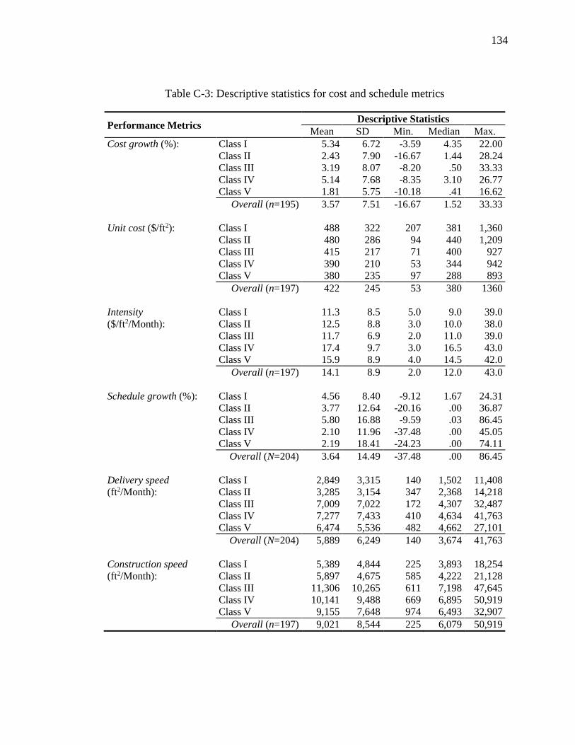
134
Table C-3: Descriptive statistics for cost and schedule metrics
Performance Metrics Descriptive Statistics
Mean SD Min. Median Max.
Cost growth (%): Class I 5.34 6.72 -3.59 4.35 22.00
Class II 2.43 7.90 -16.67 1.44 28.24
Class III 3.19 8.07 -8.20 .50 33.33
Class IV 5.14 7.68 -8.35 3.10 26.77
Class V 1.81 5.75 -10.18 .41 16.62
Overall (n=195) 3.57 7.51 -16.67 1.52 33.33
Unit cost ($/ft2): Class I 488 322 207 381 1,360
Class II 480 286 94 440 1,209
Class III 415 217 71 400 927
Class IV 390 210 53 344 942
Class V 380 235 97 288 893
Overall (n=197) 422 245 53 380 1360
Intensity Class I 11.3 8.5 5.0 9.0 39.0
($/ft2/Month): Class II 12.5 8.8 3.0 10.0 38.0
Class III 11.7 6.9 2.0 11.0 39.0
Class IV 17.4 9.7 3.0 16.5 43.0
Class V 15.9 8.9 4.0 14.5 42.0
Overall (n=197) 14.1 8.9 2.0 12.0 43.0
Schedule growth (%): Class I 4.56 8.40 -9.12 1.67 24.31
Class II 3.77 12.64 -20.16 .00 36.87
Class III 5.80 16.88 -9.59 .03 86.45
Class IV 2.10 11.96 -37.48 .00 45.05
Class V 2.19 18.41 -24.23 .00 74.11
Overall (N=204) 3.64 14.49 -37.48 .00 86.45
Delivery speed Class I 2,849 3,315 140 1,502 11,408
(ft2/Month): Class II 3,285 3,154 347 2,368 14,218
Class III 7,009 7,022 172 4,307 32,487
Class IV 7,277 7,433 410 4,634 41,763
Class V 6,474 5,536 482 4,662 27,101
Overall (N=204) 5,889 6,249 140 3,674 41,763
Construction speed Class I 5,389 4,844 225 3,893 18,254
(ft2/Month): Class II 5,897 4,675 585 4,222 21,128
Class III 11,306 10,265 611 7,198 47,645
Class IV 10,141 9,488 669 6,895 50,919
Class V 9,155 7,648 974 6,493 32,907
Overall (n=197) 9,021 8,544 225 6,079 50,919
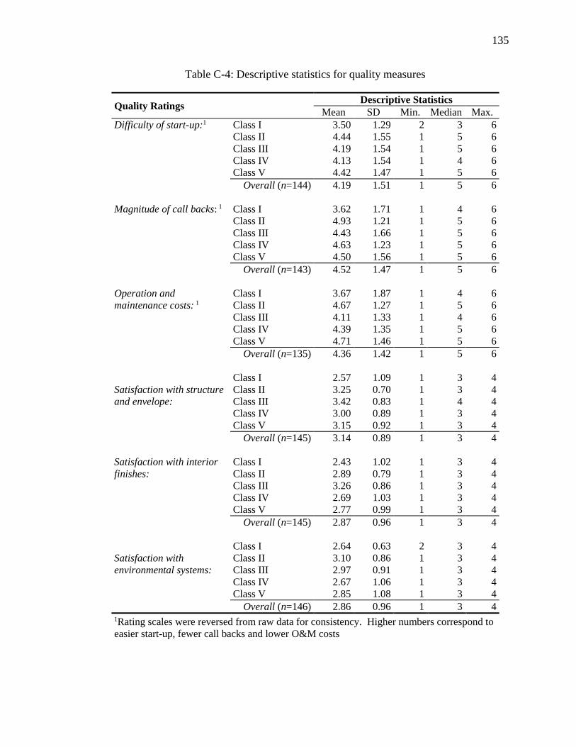
135
Table C-4: Descriptive statistics for quality measures
Quality Ratings Descriptive Statistics
Mean SD Min. Median Max.
Difficulty of start-up:1 Class I 3.50 1.29 2 3 6
Class II 4.44 1.55 1 5 6
Class III 4.19 1.54 1 5 6
Class IV 4.13 1.54 1 4 6
Class V 4.42 1.47 1 5 6
Overall (n=144) 4.19 1.51 1 5 6
Magnitude of call backs: 1 Class I 3.62 1.71 1 4 6
Class II 4.93 1.21 1 5 6
Class III 4.43 1.66 1 5 6
Class IV 4.63 1.23 1 5 6
Class V 4.50 1.56 1 5 6
Overall (n=143) 4.52 1.47 1 5 6
Operation and
maintenance costs: 1
Class I 3.67 1.87 1 4 6
Class II 4.67 1.27 1 5 6
Class III 4.11 1.33 1 4 6
Class IV 4.39 1.35 1 5 6
Class V 4.71 1.46 1 5 6
Overall (n=135) 4.36 1.42 1 5 6
Satisfaction with structure
and envelope:
Class I 2.57 1.09 1 3 4
Class II 3.25 0.70 1 3 4
Class III 3.42 0.83 1 4 4
Class IV 3.00 0.89 1 3 4
Class V 3.15 0.92 1 3 4
Overall (n=145) 3.14 0.89 1 3 4
Satisfaction with interior
finishes:
Class I 2.43 1.02 1 3 4
Class II 2.89 0.79 1 3 4
Class III 3.26 0.86 1 3 4
Class IV 2.69 1.03 1 3 4
Class V 2.77 0.99 1 3 4
Overall (n=145) 2.87 0.96 1 3 4
Satisfaction with
environmental systems:
Class I 2.64 0.63 2 3 4
Class II 3.10 0.86 1 3 4
Class III 2.97 0.91 1 3 4
Class IV 2.67 1.06 1 3 4
Class V 2.85 1.08 1 3 4
Overall (n=146) 2.86 0.96 1 3 4 1Rating scales were reversed from raw data for consistency. Higher numbers correspond to
easier start-up, fewer call backs and lower O&M costs

136
Appendix D: EXPANDED STRUCTURAL MODEL
Project
Cost Growth
Project
Sch. Growth
Delivery
Speed
Unit Cost
Difficulty of
Start-up
Magnitude of
Call Backs
O&M Costs
Structure &
Envelope
Interior
Finishes
Environmental
Systems
System
Quality
Turnover
Experience
ChemistryComm.
Timeliness
Goal
Commit.
Intensity
Construction
Speed
BIM UsesBIM Plan
Partic.
Charrette
Partic.
Colocation
Partic.
Goal Set
Partic.
Class II
Class III
Class IV
Class V
Public Owner
Facility Size
Group
Cohesiveness
Team
Integration
137
Appendix E: WHITE PAPER
138

139

140
141

142
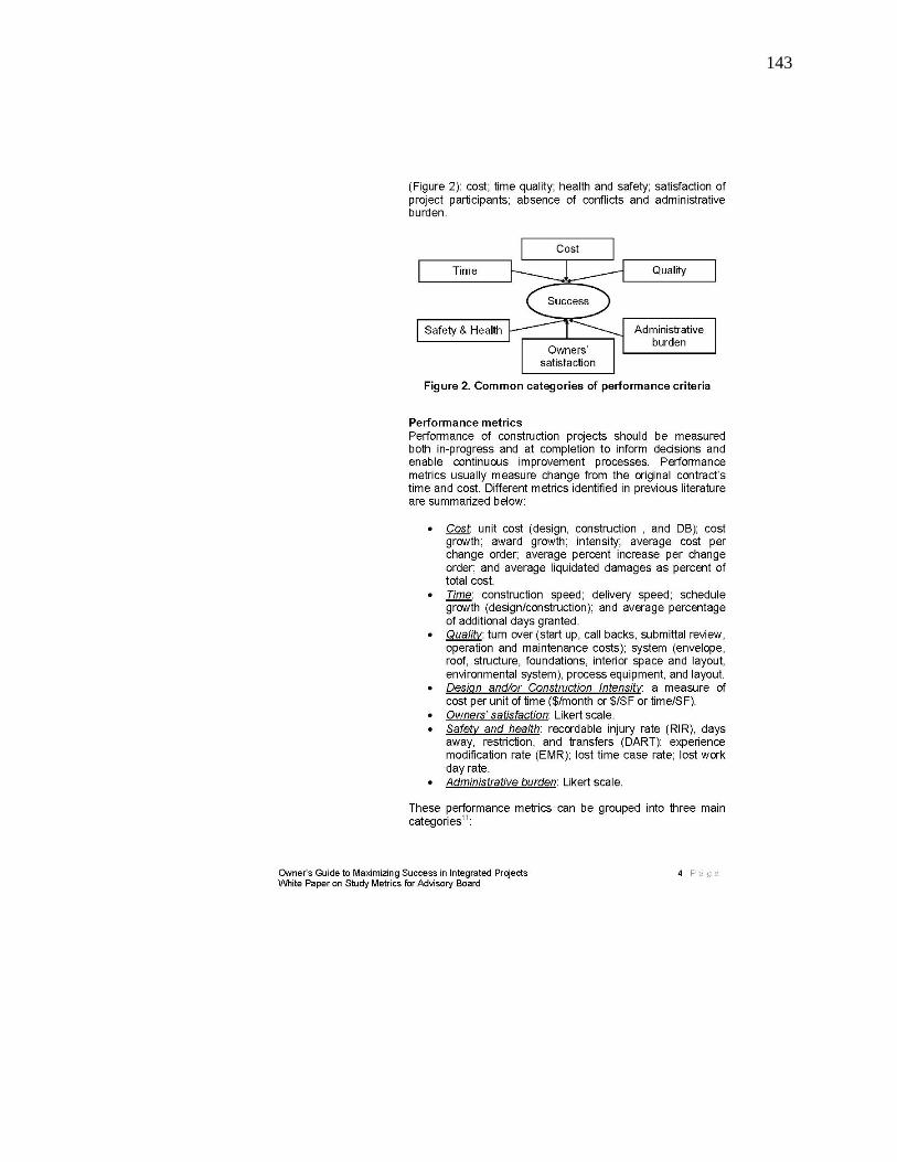
143
144

145

146
147

148
149

150

151
Appendix F: R’S GUIDE
In an effort to develop an Owner’s Guide to Integrated Projects, the process
developed in the following pages was based upon the results of an empirical study of
more than 200 completed projects. Using a variety of statistical methods to gain a full
understanding of the projects, and relationships contained therein, the main finding of the
research was that delivery decisions, (e.g. organizational structure, procurement
processes, and contractual terms) could not be made independent from one another but
need to be designed in concert, as a strategy. In particular, the strategies which aligned
the project team, through both integrated processes and development of a cohesive
group, were the only means for achieving measures of project success – cost, quality, and
schedule performance.
While the development of the team is likely not a surprising insight for many who
have experience within the construction industry, the challenge of designing team
performance into the delivery process for a project may seem more like random chance
than thoughtful strategy. Three critical elements emerged from the empirical research
which serves as the themes for enabling the more effective development of a cohesive
and integrated team through delivery strategy. Developing a team able to deliver the
desired project results was best enabled through: early involvement of the core team,
qualification based selection of team members, and transparency in cost accounting.
Early involvement, not only of the builder but of critical design-build or design-assist
specialty contractors as participants in the design process, is an essential element to
delivery of integrated project requirements. Engagement in the process was critical
before the development of the schematic design of the project to garner full value from
this approach. Early involvement is necessary to enable their participation in key
collaborative processes, such as the development of project goals, participation in design
charrettes, and the development of a BIM Execution plan. The value of participation is
not only at the front end of the process, but continued interaction through construction

152
using strategies, such as colocation and increased sharing of model information through
the lifecycle of the project, indicate the need to maintain this collaboration beyond the
early design process.
To enable the early and high quality interactions to take place amongst project team
members, the means of assembling the team by engaging the builder and specialty trades
for the project is essential. Projects with the most cohesive teams relied primarily on
qualifications submissions and interview processes to assess the quality of the team
members. The shift away from selection based on the cost of the construction scope,
toward the qualifications and team chemistry of potential collaborators, is an essential
first step to breaking down the barriers to developing an effective team. Incorporating
new team members process needs to be considered beyond the selection of firms, and
used in the on-boarding every new team member as the project continues.
Finally, the contractual terminology used by the project team needs to reinforce the
approach and strategy in aligning the interests of the team. Contracts which bring the
team together with shared risk and reward were most common in the delivery of
successful projects. In addition, the use of open book accounting processes during the
design proved critical in the development of trust amongst the project team. While most
common in the builder’s contract, the projects in the most effective class often extended
this transparency to the core team of specialty trades.
These themes—early involvement, qualification driven selection, and cost
transparency—may be incorporated into a variety of delivery strategies. The key to the
process lies in designing a strategy that enables the team processes best suited to your
project needs. The pages that follow will help you in defining your project needs and
constraints, and offer paths to improving the team capabilities through the design of a
delivery strategy; extending beyond the methods, procurement, and contract to outlining
an approach to the integrated process and team development needs for your project.
The Owner’s Guide can be accessed at: http://bim.psu.edu/delivery

153
Appendix G: DISSEMINATION PLAN
Introduction
The research team benefited from strong industry collaboration on this project. Mr.
Greg Gidez, Corporate Director for Preconstruction and Design Management Services for
Hensel Phelps Construction Co., and Dr. Mark Konchar, Vice President Business
Acquisition for Balfour Beatty Construction served as the industry champions for the
project and as co-chairs for the industry panel. Mr. Gidez is a licensed architect and is
active in the leadership of the Charles Pankow Foundation (CPF) and the Design-Build
Institute of America (DBIA). Dr. Konchar, along with Dr. Sanvido who served on the
advisory panel, were principal investigators on the 1997 project delivery study for the
Construction Industry Institute (CII), “Project delivery systems: CM at Risk, Design-
Build, Design-Bid-Build,” which has proven to be the seminal empirical study on project
delivery methods for the building design and construction industry. The co-chairs proved
to be invaluable in assisting the research team with scoping, data collection and review of
the final project results.
The research team and the co-chairs formed an industry advisory panel with leaders
from the design and construction industry. The following members actively participated
in the project:
Mr. Greg Gidez, Hensel Phelps Construction Co.
Dr. Mark Konchar, Balfour Beatty Construction
Mr. Howard W. Ashcraft, Esq., Hanson Bridgett LLP
Dr. Russell Manning, Department of Defense
Mr. Spencer Brott, Trammell Crow Real Estate Services, Inc.
Dr. John Miller, Barchan Foundation, Inc.
Mr. Bill Dean, M.C. Dean, Inc.
Mr. Brendan Robinson, U.S. Architect of the Capitol
154
Mr. Tom Dyze, Walbridge
Dr. Victor Sanvido, Southland Industries
Mr. Matthew Ellis, US Army Corps of Engineers
Mr. Ronald Smith, Kaiser Permanente
Ms. Diana Hoag, Xcelsi Group, LLC
Mr. David P. Thorman, FAIA, Former California State Architect
Mr. Mike Kenig, Holder Construction
The industry panel assisted the team with the development of the final data collection
questionnaire, helped with testing, contributed project data to the study and reviewed the
final results. They also helped the team to develop products that are ready for immediate
implementation. The research team is indebted to them for their assistance and thankful
for all of their advice.
Dissemination Accomplishments to Date
While the data collection portion of this study took longer than planned due to the
detailed nature of the data collection requirements, the research team has met all of its
dissemination goals to date. The following are papers, proceedings and presentations that
have been completed to date.
Reports
Esmaeili, B., Franz, B., Messner, J. Leicht, R. M. and Molenaar, K.R. (2012) “Owner’s
Guide to Maximizing Success in Integrated Projects: A Summary of Study
Performance Metrics,” White Paper for the Charles Pankow Foundation and the
Construction Industry Institute, November 2012.
Conference Presentation with Paper
Esmaeili, B., Pellicer, E., and Molenaar, K.R. (2014). “Critical Success Factors for
Construction Projects,” 18th International Congress on Project Management and
Engineering, Alcañiz, Spain, July 2014. (Note: this paper won the Jaume Blasco
155
Award for Innovation, the second place paper award in project management track of
the conference.)
Pellicer, E., Sanz, A., Esmaeili, B. and Molenaar, K. (2014). “Collaborative Behavior in
the Spanish Building Industry: A Preliminary Analysis,” 18th International Congress
on Project Management and Engineering, Alcañiz, Spain, July 2014.
Franz, B., Esmaeili, B., Leicht, R.M., Molenaar, K.R., Messner, J. (2014). “Exploring the
Role of the Team Environment in Building Project Performance,” 2014 ASCE
Construction Research Congress, Atlanta, GA, March 2014.
Esmaeili, B., Franz, B., Molenaar, K.R., Leicht, R.M., Messner, J., (2013). “Construction
Projects’ Performance Metrics and Critical Success Factors.” CSCE Annual
Conference (CSCE 2013), Montreal, Canada, May.
Conference Presentations
“Measuring Project Delivery Performance,” Pankow Foundation Board of Directors
Meeting, Denver, CO, June 2012.
“Project Delivery Selection,” Design-Build Institute of America Rocky Mountain Region
Annual Conference, Denver, CO, May, 2013.
“Project Delivery Performance: Lessons Learned from Vertical Construction”, 2014
Transportation Research Board (TRB) and National Institute of Building Sciences
(NIBS), AFH30: Digital Project Delivery, Washington DC, January 2014.
“Project Delivery Performance: Lessons Learned from Vertical Construction”, Project
Management Institute (PMI) Mid-Nebraska Chapter, Lincoln, NE, May 2014.

156
“Impacts of Project Delivery Methods on Project Outcomes” Construction Management
Association of America, Capital Projects Symposium, Baltimore, Maryland, May
2014.
“Project Delivery Research,” as part of the Research Trends Panel, The Design Build
Association of America, Annual Conference, Dallas, TX, November 2014.
“ Driving Innovation Through Facilitated Collaboration,” Construction Owners
Association of America, Annual Conference, November 20, 2014.
Project Website
Project Data Collection Website: https://cpf.colorado.edu
The project data collection website was developed with the intent of providing basic
project information and disseminating the project data collection survey. Additionally,
the website was used to disseminate the project
team’s white paper titled “Owner’s Guide to
Maximizing Success in Integrated Projects: A
Summary of Study Performance Metrics.” The
website proved useful for general communications
during the project.
Project Dissemination Website: http://bim.psu.edu/delivery
The project dissemination website will aid in publishing the completed project
information and the on-going owner guidance. The site design is being modeled from the
successful BIM Planning Website (http://bim.psu.edu/) that contains the BIM Project
Execution Guide, which is a similar product from a CPF/CII/Penn State research
collaboration. The website will be used to disseminate the project’s research report,
owner’s guide, project data for future researcher’s use and on-going research relating to
this study.

157
Continuing Dissemination Plan
While the project is complete, the project team remains committed to disseminating
the research through conference presentations, peer-reviewed journal publications and
dissemination of the owner’s guides through the project dissemination website.
Dissemination Focus
The focus of the project team’s continuing efforts is to facilitate owner decision
making in relation to the project delivery process. The owner group includes the facility
managers, operators and end users. Owner representatives, or agency firms, will also
receive benefit from the resources. More broadly, this research will be helpful to all
members of the construction industry. It helps to determine the various stakeholders’
responsibilities, requirements and deliverables. By utilizing the research products, the
various project team members will be better able to meet the needs of the facility owner
and end users. Furthermore, many of the industry professional organizations have
interests in the research products and will provide opportunities for dissemination at their
conferences and meetings.
Conference Presentations
The research team and members of the advisory panel are committed to “getting the
word out” through meeting and conference presentations. This has been demonstrated by
the presentations of in-progress work that has already been made. The team will now
more aggressively seek opportunities for dissemination in the coming year. The
following are conferences at which the research team is committed to present its findings
pending final acceptance of our presentation proposals.
Associated General Contractors of America Public/Private Industry Advisory
Council’s On-Line Meeting Forum, Feb 2, 2015

158
“Project Delivery Performance: The Impact of Team Selection Process”, 2015
Nebraska Architectural Engineering Conference (NAEC) - AEI/ASHRAE Expo,
Omaha, NE, March 2015
Architectural Engineering Institute – Annual Conference – Milwaukee, March 27
2015
PACE Research Seminar 2014, April, University Park, PA.
Construction Owner’s Association of America, Spring Owners Leadership
Conference, May 13-15, 2015, Baltimore, MD
Canadian Society for Civil Engineering Construction Specialty Conference, Jun
8-10, 2015, Vancouver, British Columbia
CII Annual Conference, Aug 3-5, 2015, Boston, MA
DBIA/Society of Military Engineers (SAME) Federal Project Delivery
Symposium, Aug 18-20, Washington, DC
DBIA Annual Conference and Expo, Nov 2-4, 2015, Denver, CO
Construction Management Association of America (CMAA), National
Conference & Trade Show, October 11-13, 2015, Orlando, FL
Typical Media Release(s)
Upon review of the research products by CPF and CII, the team will use media
releases to various venues to announce the research project’s purpose, results, outcomes,
and products. The releases will include the reason for the release, the projects website, as
well as a thank you to the project sponsors including the Charles Pankow Foundation and
CII. The following is an example of a typical media release:
The University of Colorado and Pennsylvania State University are pleased to
announce the release of the Owner’s Guide to Maximizing Success in Integrated
Projects. The Guide provides a practical manual to assist owners when
organizing and executing projects with integrated teams. The Guide is available
for download on the project’s website (www.xxx). The research team would like
to thank the Charles Pankow Foundation and the Construction Industry Institute
159
for their generous support of this project. We would also like to thank the more
than 200 individuals who provided empirical data for this study.
Paper in Process
The team is currently working on manuscripts for multiple peer-reviewed journals.
The goal of these publications is to share the details of the research methods, data
analysis and results with other researchers. By adding to the body of research knowledge
in the area of project delivery methods and integration, the research team hopes to spur
continued study that builds upon the findings of this research. The peer-reviewed
journals include, but are not limited to:
Journal of Management in Engineering (paper and electronic)
Journal of Construction Engineering and Management (paper and electronic)
Engineering, Construction and Architectural Management (paper and electronic)
Conclusions
The research team is aware of CPF’s and CII’s strong commitment to putting their
research results into practice. The completed and future actions described in this
dissemination plan provide evidence of the research team’s commitments to these same
goals. Although the funding for this project has been expended, the research team is
dedicated to the topic and looks forward to disseminating the findings in 2015 and
beyond. The results are expected to have a lasting impact on the industry. The results
are also expected to spur future research initiatives through a discussion of the results and
the questions that remain.
Recommended


![[Case Study] OVH main challenges and key differentiators](https://img.pdfslide.us/doc/110x75/5a672f0f7f8b9ab12b8b47b1/case-study-ovh-main-challenges-and-key-differentiators.jpg)