Model-Based ECG Fiducial Points Extraction Using a Modified EKF
Structure
Presented by: Omid Sayadi
Biomedical Signal and Image Processing Lab (BiSIPL),Biomedical Signal and Image Processing Lab (BiSIPL),Sharif University of Technology, Tehran, IranSharif University of Technology, Tehran, Iran
2
Contents:
Introduction and Problem Statement Theoretical Background Model-Based Approaches Modified EKF Structure Simulation and Results Conclusion & Future Work

3
Introduction
Heart: a hollow muscular organ which through a coordinated muscle contraction generates the force to circulate blood throughout the body.
Electrocardiogram: a graph representing the electrical activity of heart, also called ECG.
5 dominant characteristic waveforms and FPs, Single/Multiple beat features, including:
Amplitude features, Time intervals, Wave durations.
Pamp
Pdur
QRSdur
QRS-amp
STelevation
QRS+amp
RRint
QTpint
QTint
Tamp
TPint

4
Problem Statement
Arrhythmia Investigation, detection, diagnosis and treatment:
0 100 200 300 400 500 600 700 800 900-1.8
-1.6
-1.4
-1.2
-1
-0.8
-0.6
-0.4
-0.2
0
0.2
Samples
Am
plitu
de [
mV
]
200 300 400 500 600 700 800 900-1
-0.5
0
0.5
1
1.5
2
2.5
Samples
Am
plitu
de [
mV
]
0 100 200 300 400 500 600 700-0.8
-0.6
-0.4
-0.2
0
0.2
0.4
0.6
Samples
Am
plitu
de [
mV
]
Major Problems: Decision Dependency,
Variability,
Noise and Drifts,
Ischemia Sinus Bradycardia Wolf Parkinson White Branch Bundle Block (BBB) Ventricular Tachycardia (VT) Ventricular Bigeminy/Trigeminy Atrial/Ventricular Flutter (AFL/VFL) Premature Atrial Contraction (APC) Atrial/Ventricular Fibrillation (AF/VF) Premature Ventricular Contraction (PVC)
Lack of sufficient morphological information.

5
Problem Statement
Goal:
Adaptive usage of the underlying ECG dynamical mechanism. Accuracy achievement for Arrhythmia Investigation:
Beat Detection,Beat Classification,Fiducial Points Extraction, Interval Timing Calculation,Feature Generation.

6
Contents:
Introduction and Problem Statement Theoretical Background Model-Based Approaches Modified EKF Structure Simulation and Results Conclusion & Future Work

7
Theoretical Background
ECG Dynamical Model (EDM):
},,,,{02
2)(
2exp
TSRQPi i
iii zz
baz
xyy
yxx
221 yx
2mod)( ii
),(2 xyanat
-2
-1
0
1
2
-1.5-1
-0.50
0.51
1.5-0.5
0
0.5
1
1.5
xy
z [m
V]
0 500 1000 1500 2000 2500 3000 3500 4000 4500 5000
-0.4
-0.2
0
0.2
0.4
0.6
0.8
1
1.2
Samples
Am
p [
mV
]
-1.5 -1 -0.5 0 0.5 1 1.5-1.5
-1
-0.5
0
0.5
1
1.5
X
Y
250 300 350 400 450 500 550 600 650-0.4
-0.2
0
0.2
0.4
0.6
0.8
1
1.2
Time/Index
Am
plitu
de [m
V]
8
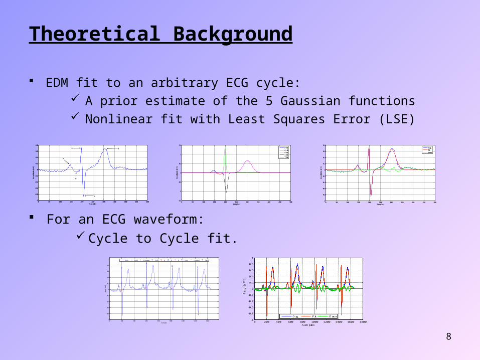
Theoretical Background
EDM fit to an arbitrary ECG cycle:A prior estimate of the 5 Gaussian functionsNonlinear fit with Least Squares Error (LSE)
0 50 100 150 200 250 300 350 400 450 500-1
-0.8
-0.6
-0.4
-0.2
0
0.2
0.4
0.6
0.8
Samples
Am
plit
ud
e [m
V]
P
Q
R
S
T
0 50 100 150 200 250 300 350 400 450 500-1.5
-1
-0.5
0
0.5
1
1.5
Samples
Am
plit
ud
e [m
V]
P fitQ fitR fitS fitT fit
0 50 100 150 200 250 300 350 400 450 500-1
-0.8
-0.6
-0.4
-0.2
0
0.2
0.4
0.6
0.8
Samples
Am
plit
ud
e [m
V]
Org.fiterror
For an ECG waveform:Cycle to Cycle fit.
0 200 400 600 800 1000 1200 1400 1600-1
-0.8
-0.6
-0.4
-0.2
0
0.2
0.4
0.6
0.8
1
Samples
Am
p [m
V]
ECG P(on) P(center) P(off) Q R S T(on) T(center) T(off)
0 200 400 600 800 1000 1200 1400 1600 1800-1
-0.8
-0.6
-0.4
-0.2
0
0.2
0.4
0.6
0.8
1
Samples
Am
p [
mV
]
Org. Fit Error

9
Contents:
Introduction and Problem Statement Theoretical Background Model-Based Approaches Modified EKF Structure Simulation and Results Conclusion & Future Work
10
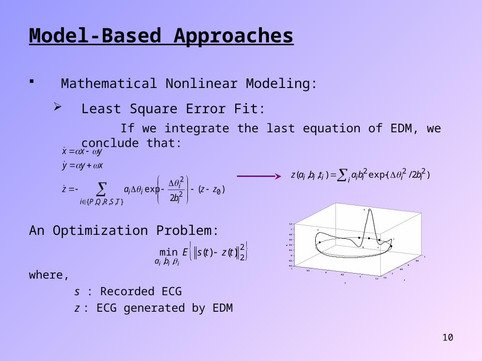
Model-Based Approaches
Mathematical Nonlinear Modeling:
Least Square Error Fit:
If we integrate the last equation of EDM, we conclude that:
i iiiiiii bbatbaz )2/exp(),,( 222
},,,,{02
2)(
2exp
TSRQPi i
iii zz
baz
xyy
yxx
An Optimization Problem: 2
2,,)()(min tztsE
iii ba
where,
s : Recorded ECG
z : ECG generated by EDM
-1.5
-1
-0.5
0
0.5
1
-1.5-1
-0.50
0.51
-0.4
-0.2
0
0.2
0.4
0.6
0.8
1
1.2
xy
N
R
P
Q S
T

11
Model-Based Approaches
Adaptive Tracking:
Considering the nonlinear underlying dynamics for estimation → Extended Kalman Filter (EKF=linearized KF)
The discrete polar form of EDM:
kTSRQPi i
ii
i
ik
kk
zbb
z
odm
},,,,{2
2
21
1
)2
exp(
)2()(
random white noise which represents the baseline wander effects and models other additive
sources of process noise
sampling period (discretization step)
result of discrete derivation:
kk
kk
xx
xx
dt
dx
...1
1
12
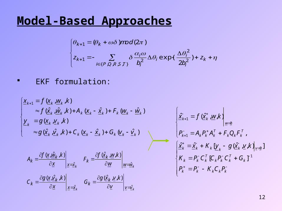
Model-Based Approaches
EKF formulation:
kTSRQPi i
ii
i
ik
kk
zbb
z
odm
},,,,{2
2
21
1
)2
exp(
)2()(
)ˆ()ˆ(),ˆ,ˆ(
),,(
)ˆ()ˆ(),ˆ,ˆ(
),,(1
kkkkkkkk
kkk
kkkkkkkk
kkk
vvGxxCkvxg
kvxgy
wwFxxAkwxf
kwxfx
kk ww
kk
xx
kk w
kwxfF
x
kwxfA
ˆˆ
),,ˆ(),ˆ,(
kk vv
kk
xx
kk v
kvxgG
x
kvxgC
ˆˆ
),,ˆ(),ˆ,(
kkkkk
kTkkk
Tkkk
vkkkkk
Tkkk
Tkkkk
wkk
PCKPP
GCPCCPK
kvxgyKxx
FQFAPAP
kwxfx
1
0
1
01
][
]),,ˆ([ˆˆ
,
),,ˆ(ˆ
13
Contents:
Introduction and Problem Statement Theoretical Background Model-Based Approaches Modified EKF Structure Simulation and Results Conclusion & Future Work

14
Modified EKF Structure
Remember the ECG Dynamical Model (EDM):
},,,,{02
2)(
2exp
TSRQPi i
iii zz
baz
xyy
yxx
EKF2 (Sameni et al 2005)
ECG and wrapped Phase of ECG → states, Gaussian parameters, angular frequency and baseline → noises,
kTSRQPi i
ii
i
ik
kk
zbb
z
odm
},,,,{2
2
21
1
)2
exp(
)2()(
0 0.5 1 1.5 2 2.5 3 3.5 4 4.5-4
-3
-2
-1
0
1
2
3
4
Time (sec)
Am
plit
ud
e (m
V)
ECGPhase
TTPTPTPk
Tkkk
bbw
zx
],,,,,,,,,,[
][
15
Modified EKF Structure
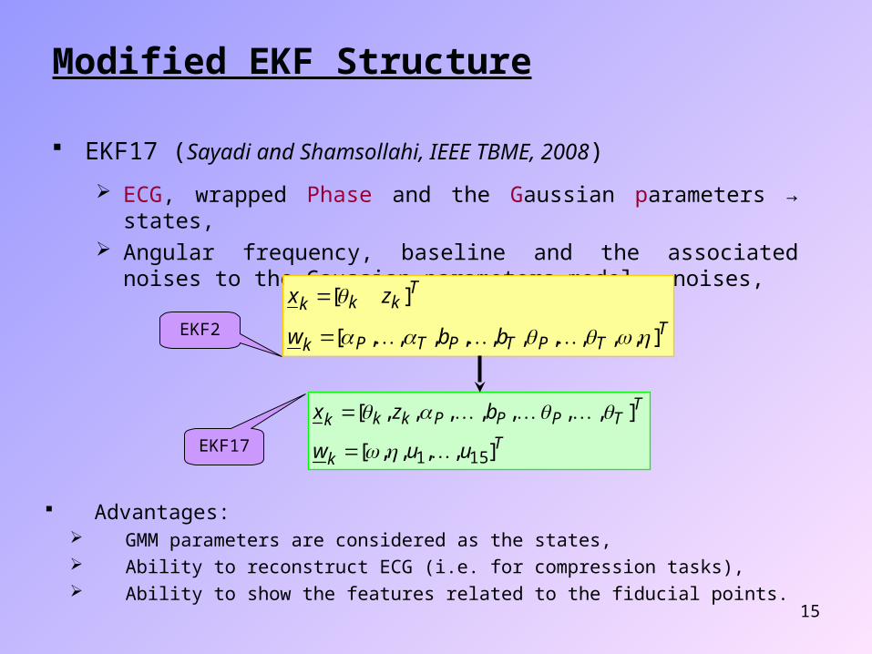
EKF17 (Sayadi and Shamsollahi, IEEE TBME, 2008)
ECG, wrapped Phase and the Gaussian parameters → states, Angular frequency, baseline and the associated noises to the
Gaussian parameters model → noises,
Advantages: GMM parameters are considered as the states, Ability to reconstruct ECG (i.e. for compression tasks), Ability to show the features related to the fiducial points.
Tk
TTPPPkkk
uuw
bzx
],,,,[
],,,,,,,[
151
TTPTPTPk
Tkkk
bbw
zx
],,,,,,,,,,[
][
EKF2
EKF17

16
Modified EKF Structure
AR(1) GMM parameters → Modified EKF (EKF17)
),,(][][]1[
),,(][][]1[
),,,,,,(][
)][2
][exp(][.
][
][.]1[
),,(.][]1[
151715
131
2
},,,,{2
2
2
1
kuFkukk
kuFkukk
kNbzFkz
kb
kk
kb
kkz
kFkk
k
k
kkk
TTT
PPP
iiikk
TSRQPi i
ii
i
i
k
Process equations:
Observation equations:
k
k
v
vx
s kk
k
2
1
0010
0001

17
Modified EKF Structure
Linearized state-space model at each time instant around the most recent state estimation:
),2
exp(]2
1[
),2
exp(]2
1[2
),2
exp(
),2
exp(]1[
2
2
2
2
22
2
2
2
2
32
2
2
22
2
2
},,,,{2
2
22
i
i
i
i
i
i
ki
i
i
i
ii
i
i
ki
i
ii
iki
i
i
TSRQPi i
i
i
i
k
bbb
F
bbbb
F
bb
F
bbb
F
.1
,1
,1
1716151413
12111098
2176543
kTkSkRkQkP
kTkSkRkQkP
kkkTkSkRkQkP
FFFFF
b
F
b
F
b
F
b
F
b
F
z
FFFFFFF

18
Modified EKF Structure
Interpretation of GMM parameters of EDM: FP extraction
),3max(
),3min(
),3max(
),3min(
),3max(
),3min(
offTTToff
onTTTon
offSsSoff
onQQQon
offPPPoff
onPPPon
fbT
fbT
fbQRS
fbQRS
fbP
fbP
Tachogram (RR-interval variability) extraction
RpeakR
fluctuative parts of the estimations

19
Contents:
Introduction and Problem Statement Theoretical Background Model-Based Approaches Modified EKF Structure Simulation and Results Conclusion & Future Work
20
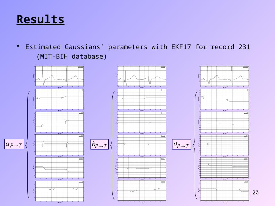
Results
Estimated Gaussians’ parameters with EKF17 for record 231
(MIT-BIH database)
1.2 1.4 1.6 1.8 2 2.2 2.4 2.6 2.8 3
-1
-0.5
0
0.5
1
1.5
Time (sec)
Am
p. (
mV
)
ECG
1.2 1.4 1.6 1.8 2 2.2 2.4 2.6 2.8 3-1
-0.8
-0.6
-0.4
-0.2
0
0.2
0.4
0.6
0.8
1
Time (sec)
Am
p. (
mV
)
P
1.2 1.4 1.6 1.8 2 2.2 2.4 2.6 2.8 30
0.2
0.4
0.6
0.8
1
1.2
1.4
1.6
1.8
2
Time (sec)
Am
p. (
mV
)
Q
1.2 1.4 1.6 1.8 2 2.2 2.4 2.6 2.8 34
4.2
4.4
4.6
4.8
5
5.2
Time (sec)
Am
p. (
mV
)
R
1.2 1.4 1.6 1.8 2 2.2 2.4 2.6 2.8 3-3
-2.5
-2
-1.5
-1
-0.5
0
0.5
1
Time (sec)
Am
p. (
mV
)
S
1.2 1.4 1.6 1.8 2 2.2 2.4 2.6 2.8 31
1.5
2
2.5
3
3.5
4
Time (sec)
Am
p. (
mV
)
T
1.2 1.4 1.6 1.8 2 2.2 2.4 2.6 2.8 3
-1
-0.5
0
0.5
1
1.5
Time (sec)
Am
p. (
mV
)
ECG
1.2 1.4 1.6 1.8 2 2.2 2.4 2.6 2.8 3
-1
-0.5
0
0.5
1
1.5
Time (sec)
Am
p. (
mV
)
ECG
1.2 1.4 1.6 1.8 2 2.2 2.4 2.6 2.8 3-2
-1.5
-1
-0.5
0
0.5
1
Time (sec)
Am
p. (
Rad
)
bP
1.2 1.4 1.6 1.8 2 2.2 2.4 2.6 2.8 3-0.2
-0.1
0
0.1
0.2
0.3
0.4
0.5
Time (sec)
Am
p. (
Rad
)
bQ
1.2 1.4 1.6 1.8 2 2.2 2.4 2.6 2.8 39
9.5
10
10.5
11
11.5
12
Time (sec)
Am
p. (
Rad
)
T
1.2 1.4 1.6 1.8 2 2.2 2.4 2.6 2.8 3-2
-1.9
-1.8
-1.7
-1.6
-1.5
-1.4
-1.3
-1.2
-1.1
-1
Time (sec)
Am
p. (
Rad
)
S
1.2 1.4 1.6 1.8 2 2.2 2.4 2.6 2.8 3
-0.25
-0.2
-0.15
-0.1
-0.05
0
0.05
0.1
0.15
0.2
Time (sec)
Am
p. (
Rad
)
R
1.2 1.4 1.6 1.8 2 2.2 2.4 2.6 2.8 3-0.5
-0.4
-0.3
-0.2
-0.1
0
0.1
0.2
0.3
0.4
Time (sec)
Am
p. (
Rad
)
Q
1.2 1.4 1.6 1.8 2 2.2 2.4 2.6 2.8 3-10
-9.9
-9.8
-9.7
-9.6
-9.5
-9.4
-9.3
-9.2
-9.1
-9
Time (sec)
Am
p. (
Rad
)
P
1.2 1.4 1.6 1.8 2 2.2 2.4 2.6 2.8 3-1
-0.5
0
0.5
1
1.5
2
Time (sec)
Am
p. (
Rad
)
bT
1.2 1.4 1.6 1.8 2 2.2 2.4 2.6 2.8 3
-0.25
-0.2
-0.15
-0.1
-0.05
0
0.05
0.1
0.15
0.2
0.25
Time (sec)
Am
p. (
Rad
)
bS
1.2 1.4 1.6 1.8 2 2.2 2.4 2.6 2.8 3-0.5
-0.4
-0.3
-0.2
-0.1
0
0.1
Time (sec)
Am
p. (
Rad
)
bR
TP TPb TP
21
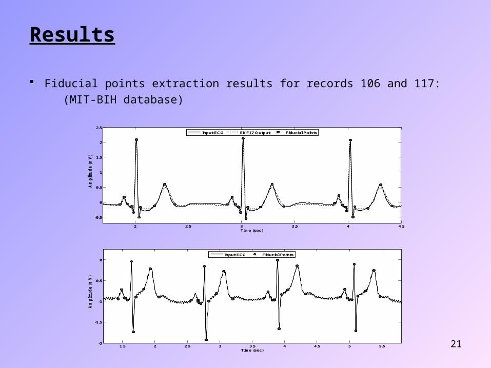
Results
Fiducial points extraction results for records 106 and 117:
(MIT-BIH database)
2 2.5 3 3.5 4 4.5
-0.5
0
0.5
1
1.5
2
2.5
Time (sec)
Am
plitu
de (
mV
)
Input ECG EKF17 Output Fiducial Points
1.5 2 2.5 3 3.5 4 4.5 5 5.5-2
-1.5
-1
-0.5
0
Time (sec)
Am
plitu
de (
mV
)
Input ECG Fiducial Points

22
Results
Numerical performance evaluation:
FNTP
TPSn
FPTN
TNSp
FPTP
TPP

23
Contents:
Introduction and Problem Statement Theoretical Background Model-Based Approaches Modified EKF Structure Simulation and Results Conclusion & Future Work
24
Conclusion
An EDM-based ECG fiducial points extraction scheme was proposed. In summary: It is very simple, very precise and has a low computational cost,
It needs a non-accurate initial estimate for the KF,
It uses the underlying dynamics for ECG signal, so it can be adapted to any ECG having five major PQRST waveforms,
No thresholding is used in determination of FPs,
There is an intrinsic denoising using the EDM, The method guarantees adaptive tracking of the morphological
characteristics of the ECG signal.
The AR(1) models provides a simple dynamics for the newly introduced state variables (i.e. GMM parameters),
The modification is applied to the process, not the observations,

25
Future Work
Fitting the model to highly abnormal ECGs such as bundle blocks,
Modifications of the model: Using more than 5 Gaussians, Modifications of the model: Using a lag-normal function, Improving the method using more precise dynamics for the
GMM parameters, instead of the AR(1), Incorporating the effects of baseline drifts.

26
Thank You ☺
Recommended