Ensemble Kalman Filter Based Data Assimilation in Wave Models

Paula Etala

Naval Hydrographic Service ∗

Pablo Echevarrıa

National Weather Service, Buenos Aires City, Argentina

1. Introduction

The continuous increase in the accuracy of operationalwave models is widely recognized. Still, there is roomfor improvement in the definition of wave conditions bymaking use of the available information globally providedby remote sensing. Lefevre (2012) showed the benefit ofsignificant wave height, wind speed and spectral observa-tions in a last-generation wave prediction system.

Since Evensen (1994) first proposed the EnsembleKalman Filter (EnKF) as an alternative to the ExtendedKalman Filter, where flow-dependent background errorswere based on an ensemble, several approaches to themodel update or analysis step have been introduced.More recently, Ott et al. (2004) proved the feasibility ofan entirely local scheme in the so-called Local EnsembleKalman Filter (LEKF) and Hunt et al. (2007) improvedthe efficiency of calculations in the Local Ensemble Trans-form Kalman Filter (LETKF). The 4D-LETKF codeshared by T. Miyoshi (Miyoshi and Yamane 2007) andupdates has been experimentally implemented in a stormsurge ensemble prediction system with very encouragingresults (Etala et al. 2012) merging altimeter and tidalgauge storm surge observations. In this article, we willdescribe an exploratory application of the same schemeto the multivariate surface vector wind and significantwave height data assimilation in a coarse NOAA/NCEPWAVEWATCH III R©(Tolman 2009) global implementa-tion.

It is widely known that in its forcing problem, wind seaquickly looses memory of its initial state. A rather short-living impact along the forecast range is then achievedby the assimilation. On the contrary, the improvement ofwind and wave mean conditions during development canprovide more long-lasting effects in the resulting swell.Improvement in the 6-hour forecast is demonstrated,although such matter is not especifically addressed for

∗Corresponding author address: Paula Etala, Naval Hydrographic

Service, Av. Montes de Oca 2124, Buenos Aires City, C1270ABV,

Argentina. Email: paulaetala@hidro.gov.ar

longer ranges in this article.

The data assimilation algorithm is described in section2, where we will briefly explain the basics of the advancedmethod used in the mean parameters analysis, as well asour approach to the update of wave spectra. The assimi-lation performed on two storm events and assesed by inde-pendent buoy data contributes to illustrate some featuresin section 3. We will discuss the results in section 4 and,finally, we will summarize conclusions and our thoughts onfuture work in section 5.

2. The Data Assimilation Method

The general approach of the EnKF combines the flow-dependent background errors provided by an ensembleprediction and the observations to build the analysisensemble, including the analysis uncertainty. The analysisensemble so obtained provides the initial state to a newensemble forecast cycle. Given an n-dimensional modelstate x and an m-member model ensemble, δXf is them × n matrix containing the m perturbations of theensemble. The ist member perturbation is defined as itsdifference to the ensemble mean δxi = xi − x. We willdenote vectors in lowercase and matrices in uppercase.

The forecast step is performed globally in the modelspace and it is common to any EnKF:

Xfi = M(Xa

i−1) (1)

Then, the forecast error covariance matrix provided by theensemble is

P f≈ (m− 1)−1δXf (δXf)T (2)

The observation operator H applied to the model variableprovides the “model observation”, i.e., the model inthe observation space yf = H(xf ). In the ensemble,δY = H(δXf) is the perturbation of the model observa-tion to the ensemble mean.

The p available observations yo introduce the newinformation in the observational increment or innovation

1

in yo − yf . The way these observations are considered inthe analysis step to update the background (section a) iswhat distinguishes LETKF from other EnKF methods.

Some localization in space and time is required to over-ride spurious background perturbations covariance, not re-lated to the local background uncertainty. An arbitrarylocal patch is defined at every analysis point where the“smoothed localization” approach increases the observa-tional error with distance to the analysis point, so that theinfluence of an observation is half its value at a distance σwhile decreasing exponentially. σ is called the “localizationscale”. The weight function 3 is applied to the inverse Rmatrix in the calculations.

W(dist) = e−dist2/2σ2

(3)

An analogous localization in time limits the observationinfluence within the assimilation window to a certain timelocalization scale. Furthermore, any corrections introducedby the observations only take place in the scale of the sig-nificant wave height (hs), zonal wind component (uw) andmeridional wind component (vw) ensemble perturbationscovariance and cross-covariance, as will be shown in sec-tion 3.

a. The analysis step: LETKF

The LETKF determines the analysis ensemble locally inthe space spanned by the ensemble, as a linear combinationof the background perturbations. Therefore, the updatedmodel state becomes:

xa = xf + (δx)fwa (4)

where w is a gaussian random vector, defined so that its en-semble mean wf = 0 and covariance P f = (k−1)−1I. Theauthors demonstrate that the solution for w also minimizesthe original analysis cost function and analysis equationsanalogous to EnKF are solved for the w ensemble in thelocal m×m ensemble space, substantially simplified by thevariable transformation.

P a = [(m− 1)I + (δY )fTR−1(δY )f ]−1 (5)

where R is the observational error covariance matrix ofthe locally used observations, modified by the localization3.

The LETKF belongs to the class of the so-called “deter-ministic” or square-root EnKF. It updates in a single stepthe ensemble mean (equation 6) and retrieves the analy-sis ensemble perturbations from the covariance matrix inequation 7.

wa = P a(δY )fTR−1(yo − yf ) (6)

δwa = [(m− 1)P a]1/2 (7)

Equations 5 to 7 for the transformation weights W arethose actually solved by the algorithm in the local spaceof the ensemble. The full analysis ensemble is then builtthrough 4 back into the global model space. Alternatively,we may choose to update the analysis mean or the deter-ministic model in a hybrid-type approach by

xa = xf + (δx)f wa (8)

The analysis ensemble perturbations in this scheme areclose to the original background ensemble perturbations,as

(δx)a = (δx)f (δw)a (9)

from 4 and 8.

b. Updating the Wave Model Spectra

Several techniques have been intended to determinethe local wave spectra from mean parameters and also toextend the impact of the assimilation along the forecastcycle. For instance, Voorrips et al. (1999) determined thewind from the wave height to use it as a smoother to thesignificant wave field. Here, we adapted the approachby Lionello et al. (1996) and Breivik and Reistad (1994),updated as in ECMWF (2013), except that we do notmake any assumptions on wind duration. Instead,weintroduce the analysed and background surface windfield into the calculations, assuming no drag change inthe analysis. We consider the total wind sea fraction asprovided by the model when splitting the analysed hs intowindsea and swell.

The updated spectrum, where f is frequency, while thef superscript denotes forecast or background, is

Ea = AEf (Bf, θ) (10)

From the dimensionless wave energy ε∗ = Eg2/u4∗ and ε∗ =

5.054∗10−4f−2.959∗ with the dimensionless mean frequency

f∗ = u∗f /g, where u∗ is the friction velocity and E =(H/4)2, being H the partitioned significant wave heightand U the wind speed, then

B =ff

fa=

(

Uf

Ua

)0.3518 (Ha

ws

Hfws

)0.6759

(11)

and

A = B

(

Haws

Hfws

)2

(12)

for the windsea part of the spectrum, and

B =

(

Hasw

Hfsw

)1

2

(13)

2

and

A = B

(

Hasw

Hfsw

)2

(14)

for the swell part of the spectrum.

The procedure described in this section completes thewind and wave data assimilation process into the wavemodel. Analysed vector wind and significant wave heightfields are the input to the assimilation routine where lo-cal 2-D spectra are inferred for every grid point using 10.The integral parameter fields and spectra after the wavespectra retrieval herein described are the final result of theassimilation and provide the ensemble restart to the newforecast cycle.

3. Experiments and results

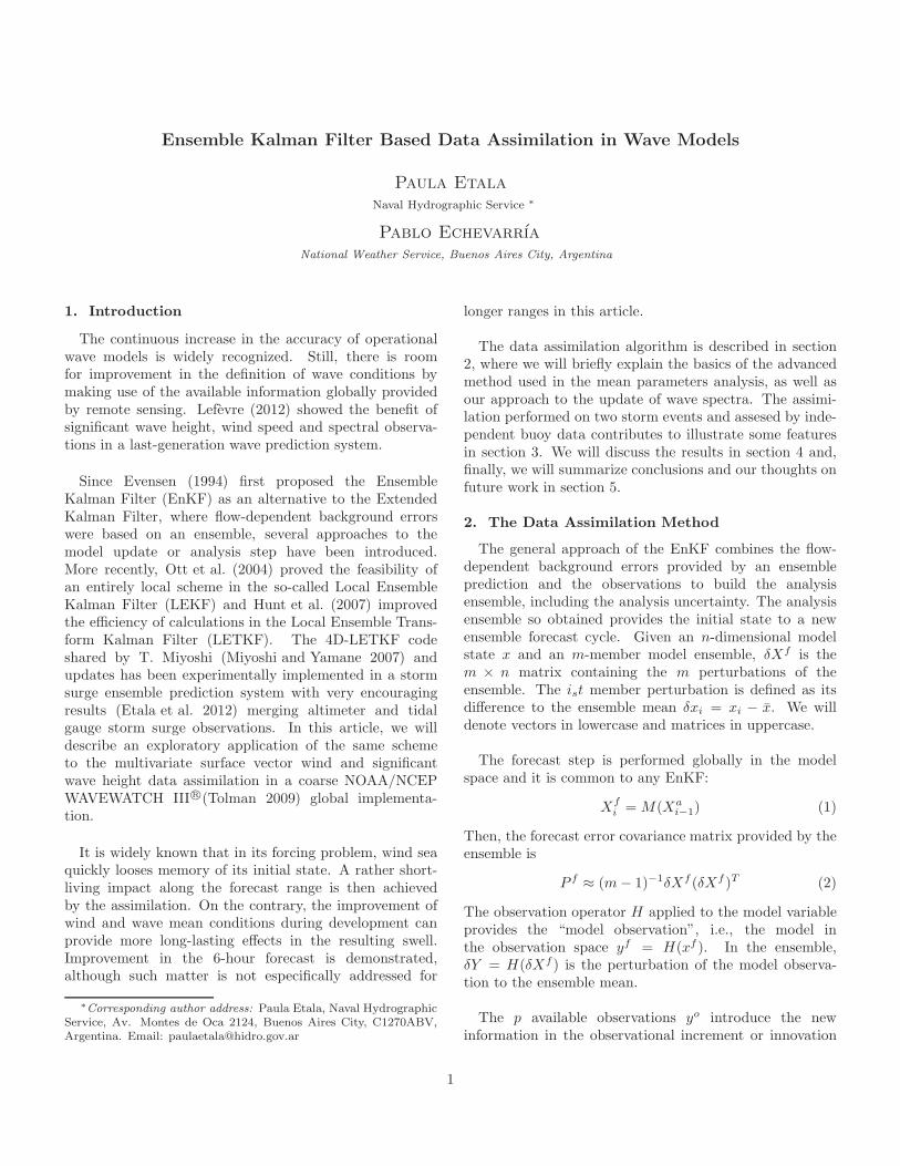
The data assimilation experiments presented in thissection correspond to the period of 17 to 29 December2012. They were set on a 6-hour ensemble forecastcycle for a global 1◦ × 1◦ WAVEWATCH III R©modelensemble. 4 daily global ensemble wind fields whereobtained from the NCEP Global Ensemble ForecastSystem (GEFS) in the THORPEX Interactive GrandGlobal Ensemble (TIGGE). Buoys available from theJCOMM Wave Forecast Verification Project (WFVP) areused here as independent data for assessment. Vector windobservations from ASCAT scatterometer and significantwave heights from altimeters on Jason 1 and Jason 2 andthe predicted model outputs were distributed in hourlyslots within every 9-hour assimilation window (T − 6hrs,T + 3hrs). Thus, the observational departure from thebackground ensemble mean (yo− yf) in equation 6, as wellas the “model observation” perturbation (δY )f reflect anevolving background field in this 4-D approach. The timelocalization scale (equation 3) used in the experiments forevery observation is 1 time slot, forward and backward.In agreement with results elsewhere, the data assimilationpresents a spin-up period of the order of 10 - 12 cycles (2.5- 3 days). In figure 1 we present the average observationaldeparture from the background ensemble mean vs. theassimilation cycle.

The localization parameter σ in equation 3 is 7◦ lat/lonin these runs, while the local patch to select the observa-tions used at each grid point is aproximately 25◦ lat/lon.The column of the error covariance matrix P f (equation2) corresponding to the point 50◦N , 140◦W is partiallyshown in figure 2 to illustrate the scale of the perturbationsin the NE Pacific storm event on 19 December 18:00. Alltimes referred are GMT. The normalized δhsδhs, δuwδhs

and δvwδhs are presented in the upper, central and lowerpanel, respectively.

Fig. 1. Evolution of the background observational depar-ture mean and standard deviation with the assimilationcycle. The observations considered are those used by theanalysis. The spin-up period was about 2-3 days (8-12 cy-cles).

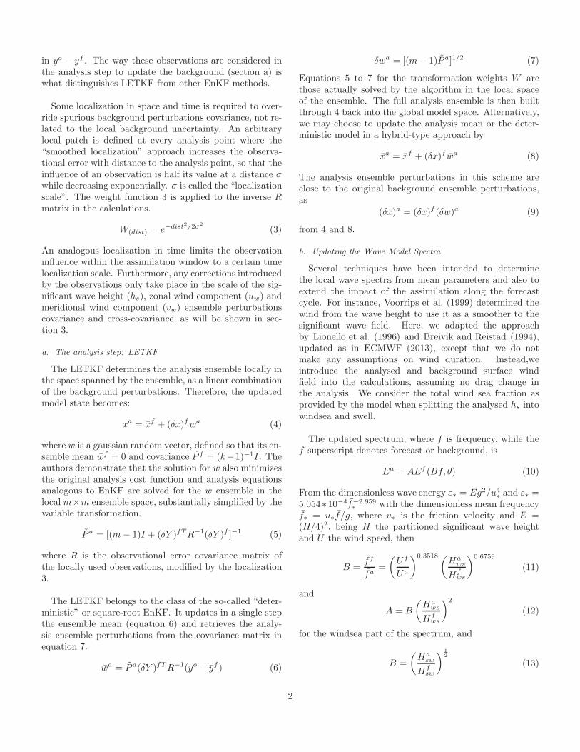
The observations used in three of the assimilation cycles,together with the hs analysis increments produced by the4D-LETKF are plotted in 3. The analysis starts correctingthe NE Pacific storm noticeably, mainly position and size,on 19 December 06:00 (upper panel). It is worth high-lighting that only wind information was available on siteat 18:00 (center panel). Figure 4 shows the 6-hour forecasthsensemble mean produced by this full-assimilation runand that from the control no-assimilation cycle at buoys46184 and 46208 offshore the Canadian West coast (buoyslocations are plotted in figure 5).

Supporting the initial correction to wave generation, thewaves generated were further updated in succeeding cyclesby the scatterometer and altimeters at day 20 00:00 (figure3lower panel) and the southward swell is still correctedby altimeters one day later (not shown). On the otherhand, the hs contrast between the full and control runstwo days later is shown in 5. The swell delay without thecycle-by-cycle analysis update is more remarkable. Buoy51101 North of Hawaii confirms these results after day 21in figure 6 (buoy location in figure 5).

Similarly, the assimilation is assessed and validated atbuoy 56006 in figure 7, Australia SW coast (buoy locationin figure 8 upper right panel). On 19 December, the 6-hourhs prediction is impacted by the overall assimilation pro-cess. Waves produced by a storm moving northeastwardalong a track located south of the continent are detected atthe western coast around 06:00. The normalized 2-D waveenergy spectra (not shown) provide evidence of the pres-ence of waves due to the storm passing south. Even though

3

Fig. 3. hs analysis increments (analysis - background) together with the altimeters and scatterometer tracks used bythe analyses in the assimilation windows for 19 December 2012 06:00, 18:00 and 20 December 2012 00:00 (upper, centerand lower panel, respectively).

4

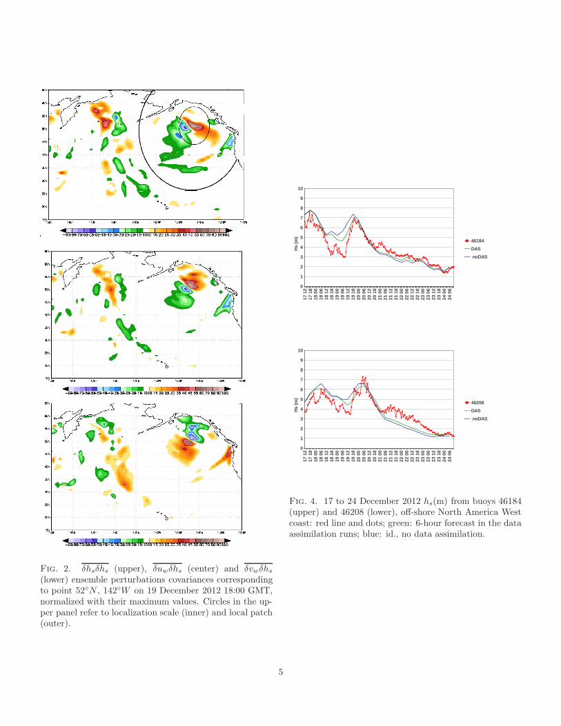
Fig. 2. δhsδhs (upper), δuwδhs (center) and δvwδhs

(lower) ensemble perturbations covariances correspondingto point 52◦N , 142◦W on 19 December 2012 18:00 GMT,normalized with their maximum values. Circles in the up-per panel refer to localization scale (inner) and local patch(outer).

Fig. 4. 17 to 24 December 2012 hs(m) from buoys 46184(upper) and 46208 (lower), off-shore North America Westcoast: red line and dots; green: 6-hour forecast in the dataassimilation runs; blue: id., no data assimilation.

5

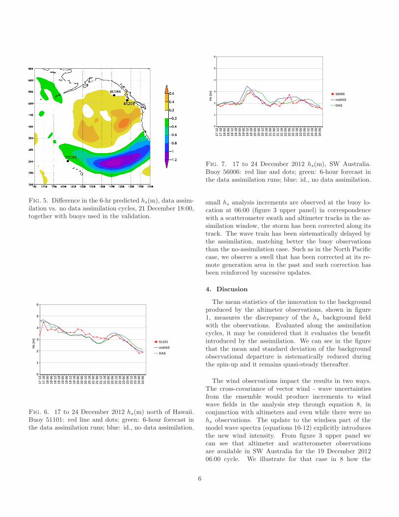
Fig. 5. Difference in the 6-hr predicted hs(m), data assim-ilation vs. no data assimilation cycles, 21 December 18:00,together with buoys used in the validation.

Fig. 6. 17 to 24 December 2012 hs(m) north of Hawaii.Buoy 51101: red line and dots; green: 6-hour forecast inthe data assimilation runs; blue: id., no data assimilation.

Fig. 7. 17 to 24 December 2012 hs(m), SW Australia.Buoy 56006: red line and dots; green: 6-hour forecast inthe data assimilation runs; blue: id., no data assimilation.

small hs analysis increments are observed at the buoy lo-cation at 06:00 (figure 3 upper panel) in correspondencewith a scatterometer swath and altimeter tracks in the as-similation window, the storm has been corrected along itstrack. The wave train has been sistematically delayed bythe assimilation, matching better the buoy observationsthan the no-assimilation case. Such as in the North Pacificcase, we observe a swell that has been corrected at its re-mote generation area in the past and such correction hasbeen reinforced by sucessive updates.

4. Discusion

The mean statistics of the innovation to the backgroundproduced by the altimeter observations, shown in figure1, measures the discrepancy of the hs background fieldwith the observations. Evaluated along the assimilationcycles, it may be considered that it evaluates the benefitintroduced by the assimilation. We can see in the figurethat the mean and standard deviation of the backgroundobservational departure is sistematically reduced duringthe spin-up and it remains quasi-steady thereafter.

The wind observations impact the results in two ways.The cross-covariance of vector wind - wave uncertaintiesfrom the ensemble would produce increments to windwave fields in the analysis step through equation 8, inconjunction with altimeters and even while there were nohs observations. The update to the windsea part of themodel wave spectra (equations 10-12) explicitly introducesthe new wind intensity. From figure 3 upper panel wecan see that altimeter and scatterometer observationsare available in SW Australia for the 19 December 201206:00 cycle. We illustrate for that case in 8 how the

6

final hs after the full assimilation process differs form theintermediate result from the 4D-LETKF. In particular,for the windsea part of the spectra, the analysed windfield and the wave field partitioning further impact theassimilation. We should note that the wind waves fieldshown in the upper right panel is only illustrative, as itcorresponds to the deterministic operational run and notto these experiments. Potential sources of error at thisstep may be the extra weight given to the backgroundthrough the conservation of the total windsea fractionand the actual wind to be considered in the partitioning.Some notable changes in storm positioning and/or windintensity found due to the scatterometer, would justify arevision thereof. Also, in some cases, the change in windspeed would support the need to consider friction velocityin equation 11.

Although we have not gone deeply into the update ofthe wave spectra in this work, we implicitly assigned anextra weight to the wind analysis by not considering anylimited wind duration in equation 11. On the other hand,as from the relatively short and disrupted time periodsrun so far, we could not conclude that the latter would bea particularly reliable parameter to be conserved from thebackground wind field. This matter should be consideredfurther.

Instead, we did find evidence of the benefit of theuse of vector wind observations in the determinationof wave generation through the improvement in stormpositioning, intensity definition and timing. The wavefields during the storm shown in NE Pacific (figure 4)were repeatedly corrected by both scatterometer andaltimeter observations (figure 3) by considering the “errorsof the day” in the background fields (figure 2). That ledus to a persistent long-term impact on the waves andswells, (figure 5) as detected by the Hawaiian buoy shownin figure 6. Although only 6-hour forecasts have beenconsidered here, it is a reasonable expectation that longerprediction ranges are also impacted in this sense. It shouldbe noted that the results presented here in the shape of a“deterministic” solution are based on the ensemble meanof the coarse wave model ensemble, which has been builtas a prototype with the only purpose of assessing theimpact of this data assimilation scheme.

Despite our preference so far to emphasize the deter-ministic approach through the ensemble mean, the wayin which this scheme provides ensemble initializationis very important to a persistent impact. The LETKFproperty in equation 7 to keep closeness of backgroundand analysis perturbations enables us to easily holdseparated restarts to the ensemble members throughoutthe runs. On the other hand, it is well known that the

abundance of satellite observations in the swath mightact to the detriment of the independence of observationerrors, hence the randomness assumption for the diagonalmatrix R in equation 5. The analysis ensemble spreadlowers in coincidence with scatterometer tracks, even whilewe used the 25-km resolution product. The spread hasbeen artificially sustained in these experiments by usingsome additive inflation (20% of the background ensemblespread) while getting results back into the model ensemblespace in equation 9.

5. Concluding remarks

We introduced an advanced method for wave dataassimilation, which we applied here to the significantwave height. The consideration of flow-dependent errors,including an evolving background error covariance matrix,and multivariate wind-wave analysis provide an up-to-dateefficient use of satellite observations, to produce realisticanalysis increments even in sparse data cross-track areas.The 4-D algorithm facilitates the consideration of theright time scale for wave evolution while incorporating thenew information (innovation) provided by asyncronousobservations in the assimilation window. The applica-tion of an EnKF approach makes the method and itsimplementations independent from the prediction model,hence, from model changes. The latter property makes itparticularly suitable for operational use.

The joint use of wind and wave observations allowed usto avoid some assumptions in the wave spectra retrieval,even though we have introduced an extra influence ofthe analysed wind, beyond the multivariate analysis ofwind and wind waves. Even while this algorithm canbe improved, the need to infer the whole spectra fromintegral parameters is a very weak point of every dataassimilation system, unless more complete sources ofspectral information can be made available. In this sense,we suggest that the most promising ways of improvementshould be explored by using the spectral partitioningcapability in the WAVEWATCH III R©model.

Preliminary results are encouraring, but extensivetesting and further enhancement are still needed in thescheme. Improved ways to make use of the analysed windsin the wave model shoud be explored. For instance, forcingthe model with the new winds at any previous step fromthe assimilation, could lead to a more realistic wind seafraction in the partition of the analysed significant waveheight for the spectrum update.

The immediately following step would be to also updatethe deterministic model, as in the usual approach in hybrid

7

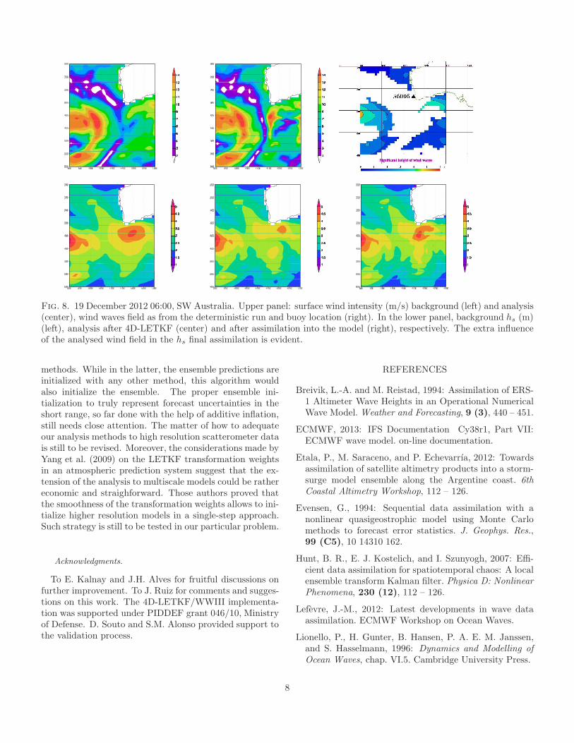
Fig. 8. 19 December 2012 06:00, SW Australia. Upper panel: surface wind intensity (m/s) background (left) and analysis(center), wind waves field as from the deterministic run and buoy location (right). In the lower panel, background hs (m)(left), analysis after 4D-LETKF (center) and after assimilation into the model (right), respectively. The extra influenceof the analysed wind field in the hs final assimilation is evident.

methods. While in the latter, the ensemble predictions areinitialized with any other method, this algorithm wouldalso initialize the ensemble. The proper ensemble ini-tialization to truly represent forecast uncertainties in theshort range, so far done with the help of additive inflation,still needs close attention. The matter of how to adequateour analysis methods to high resolution scatterometer datais still to be revised. Moreover, the considerations made byYang et al. (2009) on the LETKF transformation weightsin an atmospheric prediction system suggest that the ex-tension of the analysis to multiscale models could be rathereconomic and straighforward. Those authors proved thatthe smoothness of the transformation weights allows to ini-tialize higher resolution models in a single-step approach.Such strategy is still to be tested in our particular problem.

Acknowledgments.

To E. Kalnay and J.H. Alves for fruitful discussions onfurther improvement. To J. Ruiz for comments and sugges-tions on this work. The 4D-LETKF/WWIII implementa-tion was supported under PIDDEF grant 046/10, Ministryof Defense. D. Souto and S.M. Alonso provided support tothe validation process.

REFERENCES

Breivik, L.-A. and M. Reistad, 1994: Assimilation of ERS-1 Altimeter Wave Heights in an Operational NumericalWave Model. Weather and Forecasting, 9 (3), 440 – 451.

ECMWF, 2013: IFS Documentation Cy38r1, Part VII:ECMWF wave model. on-line documentation.

Etala, P., M. Saraceno, and P. Echevarrıa, 2012: Towardsassimilation of satellite altimetry products into a storm-surge model ensemble along the Argentine coast. 6th

Coastal Altimetry Workshop, 112 – 126.

Evensen, G., 1994: Sequential data assimilation with anonlinear quasigeostrophic model using Monte Carlomethods to forecast error statistics. J. Geophys. Res.,99 (C5), 10 14310 162.

Hunt, B. R., E. J. Kostelich, and I. Szunyogh, 2007: Effi-cient data assimilation for spatiotemporal chaos: A localensemble transform Kalman filter. Physica D: Nonlinear

Phenomena, 230 (12), 112 – 126.

Lefevre, J.-M., 2012: Latest developments in wave dataassimilation. ECMWF Workshop on Ocean Waves.

Lionello, P., H. Gunter, B. Hansen, P. A. E. M. Janssen,and S. Hasselmann, 1996: Dynamics and Modelling of

Ocean Waves, chap. VI.5. Cambridge University Press.

8

Miyoshi, T. and S. Yamane, 2007: Local Ensemble Trans-form Kalman Filtering with an AGCM at a T159/L48Resolution. Monthly Weather Review, 135 (11), 3841–3861.

Ott, E., et al., 2004: A Local Ensemble Kalman Filter forAtmospheric Data Assimilation. Tellus, 56A, 415–428.

Tolman, H. L., 2009: User manual and system documenta-tion of WAVEWATCH III version 3.14. Technical Note276, NOAA/NWS/NCEP/MMAB.

Voorrips, A. C., A. W. Heemink, and G. J. Komen, 1999:Wave data assimilation with the Kalman filter. Journalof Marine Systems, 19 (4), 267 – 291.

Yang, S.-C., E. Kalnay, B. Hunt, and N. E. Bowler, 2009:Weight interpolation for efficient data assimilation withthe Local Ensemble Transform Kalman Filter. Quarterly

Journal of the Royal Meteorological Society, 135 (638),251–262.

9