UNCERTAINTY ON TRAVEL TIME IN KINEMATIC WAVE CHANNEL ROUTING

Y.K. Tung

Symposium Proceedings 1989

WWRC - 8 9 - 30

In

Channel Flow and Catchment Runoff Proceedings of the International Conference

Kuichling's Rational Formula for Centennial of Manning's Formula and

Y.K. Tung Wyoming Water Research Center

University of Wyoming Laramie, Wyoming

767

i

I

UNCERTAINTY ON TRAVEL TIME IN KINEMATIC WAVE CHANNEL ROUTING

Yeou-Koung Tung, Assoc. Professor Wyoming Water Research Center and Statistics Department University of Wyoming Laramie, WY 82071

ABSTRACT

Channel flow routing provides information on the movement of flood wave as it travels downstream. From the flood forecast viewpoint, it is desirable to have some knowledge about the expected arrival time of peak flow. However, many parameters involved in the flow routing model, in reality, can not be quantified with certainty. In this paper, a probabilistic analysis using the Mellin transform is performed to assess the uncertainty in computing the travel time of flood wave based on the kinematic wave model. Information about the uncertainty of the arrival time of flood peak may have a potential impact on decision making relating to various contingency plans in attempting to alleviate the potential flood damage.

INTRODUCTION

Channel flood routing is an important hydraulic engineering practice because it deals with the modeling of movement of flow along the channel over time. Results of channel flow routing provide information regarding to the temporal and spatial distributions of flood wave which is essential f o r flood warning and protection.

Mathematical models used in channel flood routing range from very sophisticated 3D distributed-parameter models such as the St. Venant full dynamic wave equation to the simple lump- parameter Muskingum model (Chow et al., 1988). Intuitively, a sophisticated model not only is expansive and difficult to use, but a l s o it requires a large amount of data with reasonable accuracy in order to produce reliable results. The selection of an appropriate model to use would generally be dictated by a number of factors such as objectives of the study, accuracy requirements, data availability, budget and time constraints, and others. The solution to a channel flood routing model is a function of hydrologic characteristics of the channel such as roughness, slope, channel geometry and boundary conditions.

Deterministic analysis of channel flood routing would assume that a l l model parameters, boundary conditions and initial conditions are known with certainty. Such idealizations, in

i

768

general, are not true because the hydraulic characteristics of channels in the model constantly vary both in time and in space. Therefore, the uncertainty in model parameters would be carried through, the computation and appear in the solution.

Uncertainty in hydraulic computation for water flowing through or passing a hydraulic structure can broadly be classified into three types (Tung and Mays, 1980): model uncertainty, parameter uncertainty, and uncertainty in operational conditions of hydraulic structures. Model uncertainty results from the use of a simplified hydraulic equation to describe a complex flow phenomenon. Parameter uncertainty arises from the inaccuracy associated with the quantification of model parameters. Uncertainty in operational conditions of hydraulic structures relates to the progressive change over time of hydraulic characteristics of the structures due to sedimentation and clogging that might change the effective opening size of hydraulic structure. For flood routing in a natural channel, the uncertainty in operational conditions could be lumped into the category of parameter uncertainty.

Uncertainty analyses of hydraulic computations in channel flood routing are mainly concerned with the assessment of the uncertainty feature of the computation results. In channel flood routing, the results of primary interest are the travel time of flood peak, the magnitude of peak and corresponding water surface profile along with the area of inundation. This paper examines the uncertainty of the travel time derived from using the kinematic wave routing procedure. The method of uncertainty analysis employed is called the Mellin transform.

KINEMATIC WAVE MODEL

The kinematic wave model describes flood wave motion without considering the influence of mass and hydrodynamic force. It is a simpler version than the full dynamic wave model but still is regarded as a distributed-parameter model. The 1D kinematic wave model is defined by the following coupled equations:

3Q a A

ax at Continuity: + = q

Momentum: so = s, (lb)

where Q and A are discharge and flow cross-sectional area, respectively, which are function of both spatial location x and time t, q is the lateral inflow, and So and S, are channel bottom slope and frictional slope, respectively. Sometimes, the momentum equation can also be expressed in the form

7 6 9

~ = a Q d

Many of the well-known hydraulic equations such as Manning's formula can be expressed as Eq. 2 , Utilizing Eq.2, the continuity equation, although originally involving t w o dependent variables, A and Q, can be reduced to

( 3 ) b X

In theory, the kinemat'ic wave should advance downstream with its rising limb getting steeper. However, the s i ze of the wave does not become longer, or attenuated, Therefore, the peak of flood stays the same (Chow et ale, 1988).

The kinematic wave model can be solved by using the finite differehce scheme or t h e method of characteristics, For a problem with simpler boundary and initial conditions, kinematic wave routing can be performed analytically. For example, in case that q=O and a, B values are known, t h e outflow hydrograph at the downstream end from routing an inflow hydrograph can be easi ly obtained by shifting the inflow discharge by a t i m e interval of L/ck where c k is the wave celerity, dx/dt. In other words, a discharge Q entering a channel of length L a t time t, will appear at the outlet at time

It can be easily proved that, using Manning's formula, the travel time T of a kinematic wave in a wide rectangular channel carrying a flow of Q is (Chow et al., 1988)

3

T = - 5 [ ly41 y12 ] Q-2'5 L (6)

where B is the channel width, n is the Manning's roughness, and L is the length of channel reach.

UNCERTAINTY ANALYSIS OF TRAVEL TIME

In facing major flood events, the local authority in charge of natural disaster emergency management might consider issuing an evacuation warning, The timings of announcing the warning and of implementing the evacuation would indeed cause public inconvenience even if the threat is imminent. The prediction of the a r r iva l time of a major flood can be made by solving a flood routing model. However, due to the existence of various hydraulic uncertainties as described previously, the arrival time of a flood is generally n o t certain, The purpose of uncertainty

770

analysis of the travel time is to assess its random nature.

Uncertainty characteristics of the travel time can generally be defined by its statistical moments such as the mean, variance, and other higher moments if necessary. The complete derivation of the probability density function (pdf) as the function of pdf's of model parameters with uncertainty is generally very difficult, if not impossible. Using Eq. 6 as an example, the uncertainty of T is a function of uncertainties in n, B, so, Q, and L which are related in the multiplicative fashion. One commonly used method for assessing the statistical moments in the uncertainty analysis is the first-order second-moment (FOSM) (Benjamin and Cornell, 1970; Ang and Tang, 1975; Yen et al., 1986. However, the FOSM analysis only gives approximations of the mean and variance instead of their exact values. When higher order moments are needed, the FOSM method would become computationally cumbersome as the order gets larger. There are evidences showing that when the nonlinearity of the functional form gets higher the accuracy of approximation by the FOSM method would get worse, especially for high order moments (Tung and Hathhorn, 1988) .

Consider a general functional relationship between a dependent random variable Y and a number of independent random variables 25 =(X1, X,, r . . . , Xk) as

If the functional relation Eq.7 satisfies two conditions, the exact moments of any order can be derived by the Mellin transform as the function of moments of X ' s without extensive ,simulation. The two conditions are: (1) function u(X) has a multiplicative form as Eq.6 and (2) random variables X's are independent, non- negative. In general, the non-negativity condition of Xfs is not strictly required in the Mellin transform; but it would require some mathematical manipulations to find the Mellin transform of a function with its variables that can take negative values. The Mellin transform is particular attractive in uncertainty analysis of hydrologic and hydraulic problems because many equations and the variables involved satisfy the above two conditions.

MOMENTS AND MELLIN TRANSFORM

Statistical Moments:

The statistical moment of order r of a random variable X about any reference point X=x, is defined as

p: = E[(X-x,)'] = (x-x,) f (x) dx

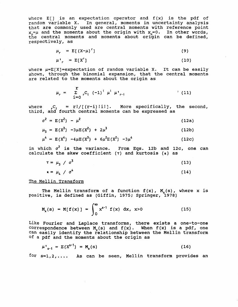
where E [ J is an expectation operator and f ( x ) is the pdf of random variable X. In general, moments in uncertainty analysis that are commonly used are central moments with reference point x0=p and the moments about the origin with x0=O. In other words, the central moments and moments about origin can be defined, respectively, as

where p=E[X]=expectation of random variable X. It can be easily shown, through the binomial expansion, that the central moments are related to the moments about the origin as

r

i=o P, = c ,Ci (-l)i pi

where , C = r!/ [ (r-i) ! i! 3. More specifically, the second, third, and fourth central moments can be expressed as

E(X*) - p2 (=a) 0 2 =

(12b) p3 = E(X3) -3pE(X2) + 21.1 3

p4 = E(X4) -4pE(X3) + 6p2E(X2) -3p4

in which o2 is the variance. From Eqs. 12b and 12c, one can calculate the skew coefficient ( 7 ) and kurtosis (K) as

7 = p3 / o3

K = p4 / O4

(13)

( 1 4 )

The Mellin Transform

The Mellin transform of a function f(x), Mx(s), where x is positive, is defined as (Giffin, 1975; Springer, 1978)

M J s ) = M[f(x)] = f(x) dx, x>O

Like Fourier and Laplace transforms, there exists a one-to-one correspondence between Mx(s) and f (x) . When f (x) is a pdf, one can easily identify the relationship between the Mellin transform of a pdf and the moments about the origin as

= E(XS-l) = M J s ) (16)

f o r s=1,2, .... As can be seen, Mellin transform provides an

772

! i

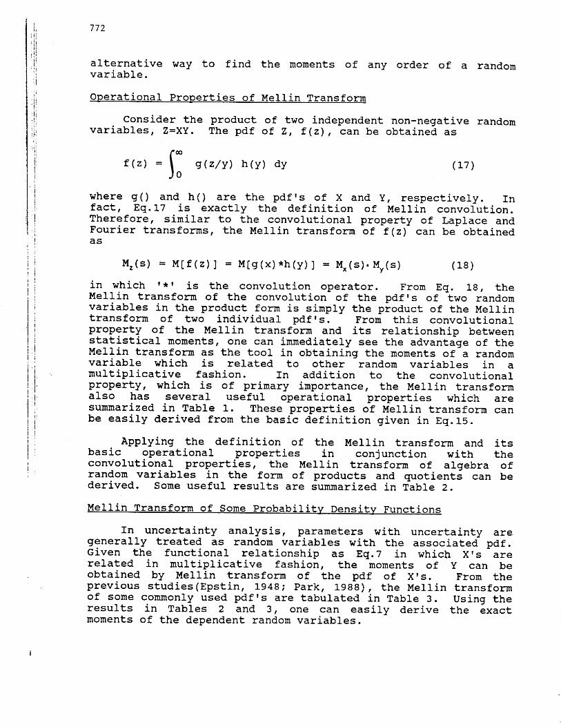
alternative way to find the moments of any order of a variable.

ODerational Properties of Mellin Transform

Consider the product of two independent non-negative variables, Z=XY. The pdf of 2, f(z), can be obtained as

random

random

where g() and h() are the pdf's of X and Y, respectively. In fact, Eq.17 is exactly the definition of Mellin convolution. Therefore, similar to the convolutional property of Laplace and Fourier transforms, the Mellin transform of f(z) can be obtained as

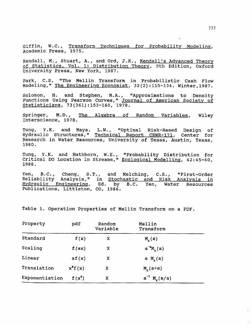
in which ' * ' is the convolution operator. From Eq. 18, the Mellin transform of the convolution of the pdf's of two random variables in the product form is simply the product of the Mellin transform of two individual pdf s . From this convolutional property of the Mellin transform and its relationship between statistical moments, one can immediately see the advantage of the Mellin transform as the tool in obtaining the moments of a random variable which is related to other random variables in a multiplicative fashion. In addition to the convolutional property, which is of primary importance, the Mellin transform also has several useful operational properties which are summarized in Table 1. These properties of Mellin transform can be easily derived from the basic definition given in Eq.15.

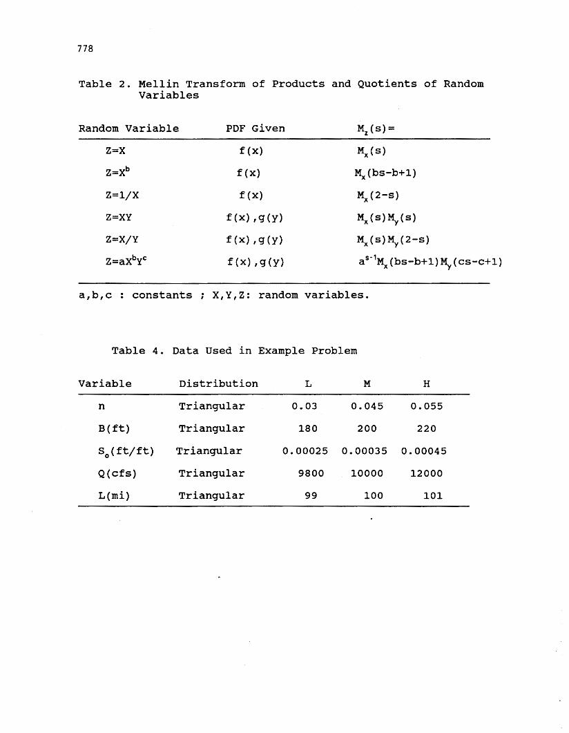
Applying the definition of the Mellin transform and its basic operational properties in conjunction with the convolutional properties, the Mellin transform of algebra of random variables in the form of products and quotients can be derived. Some useful results are summarized in Table 2 .

Mellin Transform of Some Probabilitv Density Functions

In uncertainty analysis, parameters with uncertainty are generally treated as random variables with the associated pdf. Given the functional relationship as Eq.7 in which X ' s are related in multiplicative fashion, the moments of Y can be obtained by Mellin transform of the pdf of XIS. From the previous studies(Epstin, 1948; Park, 1988) , the Mellin transform of some commonly used pdf's are tabulated in Table 3 . Using the results in Tables 2 and 3 , one can easily derive the exact moments of the dependent random variables.

I

773

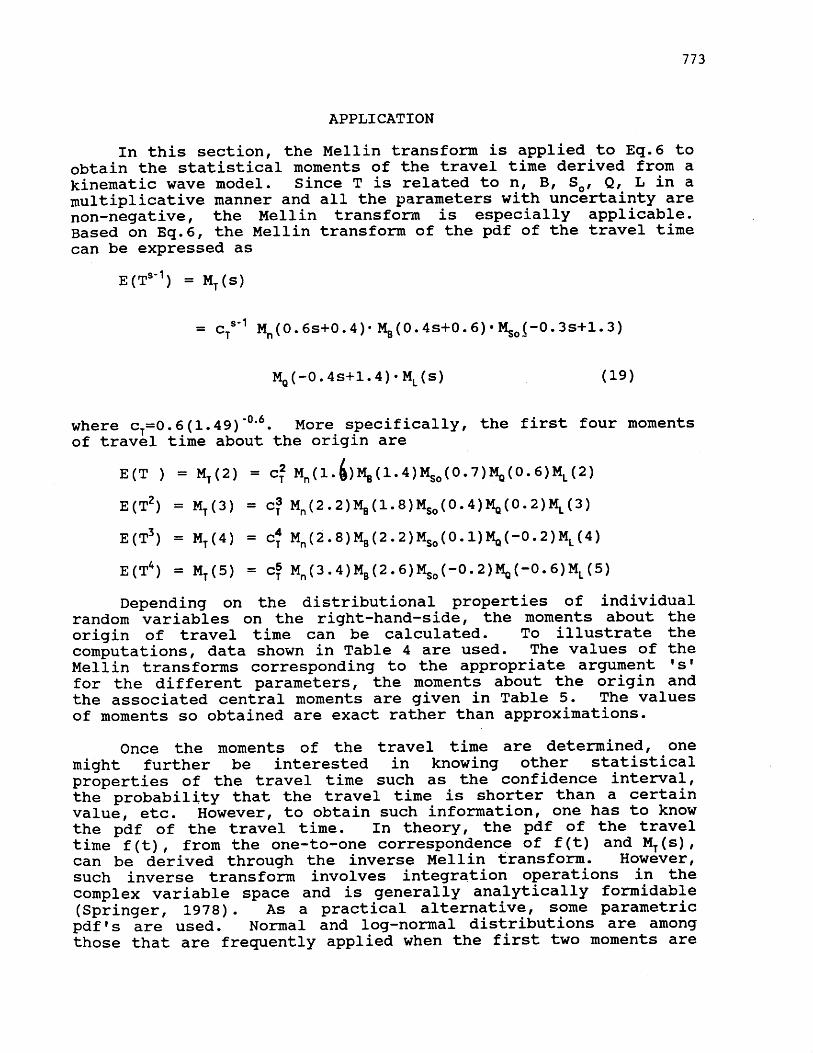
APPLICATION

In this section, the Mellin transform is applied to Eq.6 to obtain the statistical moments of the travel time derived from a kinematic wave model. Since T is related to n, B, So, Q, L in a multiplicative manner and all the parameters with uncertainty are non-negative, the Mellin transform is especially applicable. Based on Eq.6, the Mellin transform of the pdf of the travel time can be expressed as

s- 1 = CT M, ( 0 . 6~+0.4 ) % ( 0 . 4 s+O .6) qo - (-0 . 3s+l. 3 )

Ma (-0.4s+l. 4) M, (s) (19)

where ~,=0.6(1.49)-~'~. of travel time about the origin are

More specifically, the first four moments

E ( T ) = MT(2) = c: M,(l.~)MB(1.4)Mso(0.7)~(0.6)ML(2)

E(T2) = MT(3) = C; M,(2.2)M,(1.8)Mso(~.4)~(~=2)ML(3)

E (T4) = M, (5) = C? M,( 3. 4)MB (2. 6)Mso(-0. 2 ) % ( - 0 . 6)ML (5)

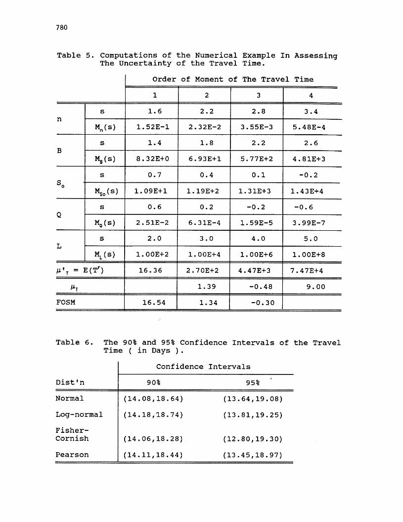
Depending on the distributional properties of individual random variables on the right-hand-side, the moments about the origin of travel time can be calculated. To illustrate the computations, data shown in Table 4 are used. The values of the Mellin transforms corresponding to the appropriate argument Is' for the different parameters, the moments about the origin and the associated central moments are given in Table 5. The values of moments so obtained are exact rather than approximations.

Once the moments of the travel time are determined, one might further be interested in knowing other statistical properties of the travel time such as the confidence interval, the probability that the travel time is shorter than a certain value, etc. However, to obtain such information, one has to know the pdf of the travel time. In theory, the pdf of the travel time f (t) , from the one-to-one correspondence of f (t) and MT (s) , can be derived through the inverse Mellin transform. However, such inverse transform involves integration operations in the complex variable space and is generally analytically formidable (Springer, 1978). As a practical alternative, some parametric pdf's are used. Normal and log-normal distributions are among those that are frequently applied when the first two moments are

774

sufficient to characterize them. This paper also includes two additional distributions to compute the quantile of the travel time associated with a given probability level: Fisher-Cornish asymptotic expansion and Pearson distributions.

Fisher-Cornish expansion approximates any distribution by the normal distribution with correction given to the presence of higher .moments such as skew coefficient , kurtosis , and etc. , which are not equal to those for normal random variables (Fisher and Cornish, 1960: Kendall et al. , 1987). The quantile of the travel time associated with a probability level p using the Fisher-Cornish expansion, truncated up to the fourth term, is

in which zp is the pth-order quantile from standard normal distribution, Hr(zp) is the Hermite polynomials which can be computed by (Abramowitz and Stegun, 1970) :

+ 0 . . (21) Xr-6 r4 r6

Xr-4 - r2 H'(x) = xr - Xr-2 +

2 l! 22 2! 23 31

As can be seen, using only the first two moments, the Fisher- Cornish expansion reduces to the normal distribution.

The Pearson distribution is a four-parameter distribution with its pdf satisfying the following limiting form

df (x-a) f

dx - -

b, + b,x + b2x2' The Pearson distribution is a very general distribution which encompass the majority of the parametric pdfls that have been commonly used. Distributions such as normal, gamma, and beta are the members of the Pearson family. The type of distribution in the Pearson system can be determined on the basis of the values of skew coefficient and kurtosis. A chart has been prepared for that purpose (Kendall et al., 1987) . Parameters in Eq.22 can be determined by relating them to the first four moments (Kendall et al. , 1987). However, it should be noted that there exist boundaries for the combinations of skew coefficient and kurtosis beyond which Pearson system of distribution does not exist. To solve the general Pearson system such as Eq.22, Bowman and Shenton (1979 a,b) have developed accurate approximations for the percentage points of the Pearson distributions using ratios of polynomials in skew coefficient and kurtosis. Recently, a computer code based on the works of Bowman and Shenton (1979a,b) was developed by Davis and Stephens (1983).

775

The main reason for using the Fisher-Cornish and Pearson distributions is that the third and the fourth moments calculated from the Mellin transform are exact values rather than approximations or estimated from the sample data. Solomon and Stephens (1978) showed that the Pearson distribution gives an excellent approximation to the long tail of a distribution when the first four moments are known exactly.

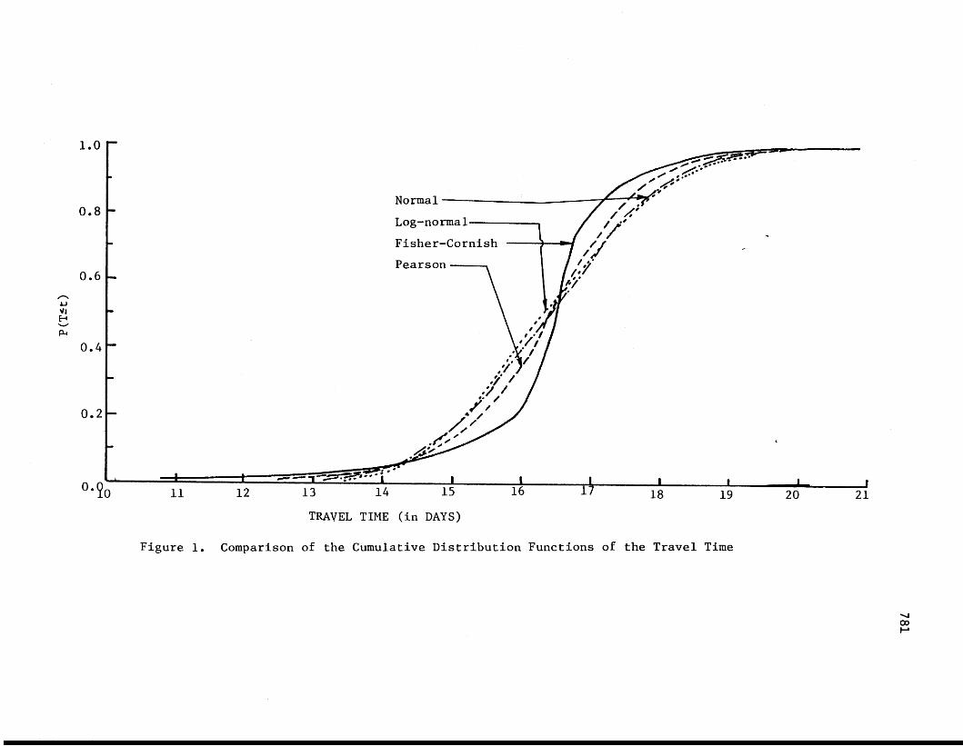
Based on Table 5, it is observed that the travel time resulting from the data in Table 4 is not normal because its skew coefficient is not zero and kurtosis is not 3 . In fact, it is negatively skewed which indicates that the distribution of the travel time is not log-normal either. For purpose of comparison, the 90% and 95% confidence intervals as well as the shape of cdf's of the travel time derived from different distributional assumptions are shown in Table 6 and Figure 1, respectively.

Compare the last two rows of Table 5, the expected flood arrival time estimated by the FOSM method is about 4 hours later than that of estimated by the Mellin transform. The standard deviation and skew coefficient by the FOSM method, however, are slightly smaller than those calculated by the Mellin transform. For this particular example, the use of FOSM method with the adoption of a normal or lognormal distribution as commonly done might not be appropriate because the skew coefficient of the travel time is negative.

CONCLUSIONS

In facing a major flooding event of which the consequence could be significant, the knowledge about the uncertainty characteristics of the flood arrival time is crucial in decision making relating to disaster averting activities such as flood warning, implementation of evacuation, and others. Examining the 95% confidence intervals of the flood travel time associated with the numerical example, the differences in the lower end points range from 4 to 24 hours with 1 to 8 hours in the upper end points. The uncertainty in the flood arrival time is about 3 3 hours. In reality, an error in predicting the flood arrival time for just one hour or less during major event could be vital to those individuals at risk.

This paper applies a useful mathematic technique called the Mellin transform to assess the statistical moments of the flood travel time derived from the kinematic wave model under some simple boundary conditions. The Mellin transform is especially attractive and simple to use when the dependent random variable is related to a number of independent random variables in multiplicative manner. Under such circumstances, exact values of the moments of any order can be derived with simple algebraic manipulations. In fact, many equations in hydrologic and hydraulic computations are of this nature to which the Mellin transform is applicable.

776

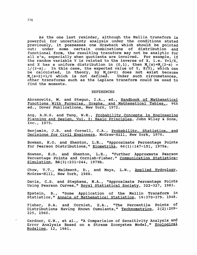
As the one last reminder, although the Mellin transform is powerful for uncertainty analysis under the conditions stated previously, it possesses one drawback which should be pointed out: under some certain combinations of distribution and functional form, the resulting transform may not be analytic for all s ' s , especially when quotients are involved. For example, if the random variable Y is related to the inverse of X, i.e. Y = l / X , and X has a uniform distribution in ( 0 , l ) , then M (s)=M ( 2 - s ) = 1 / ( 2 - s ) . In this case, the expected value of Y, ETY) , wkch can be calculated, in theory, by M ( s = 2 ) does not exist because M ( s=2)=1 /0 which is not define& Under such circumstances, &her transforms such as the Laplace transform could be used to find the moments.

REFERENCES

Abramowitz, M. and Stegun, LA., ed., Handbook of Mathematical Functions With Formulas, Graphs, and Mathematical Tables,, 9th ed., Dover Publications, New York, 1972.

Ang, A.H.S. and Tang, W.H., Probability Concepts in Ensineerinq Planninq and Desisn, Vol. I: Basic Principles, John Wiley iS Sons, Inc., 1975 .

Benjamin, J.R. and Cornell, Decisions for Civil Ensineers

C I

. A * , Probability, Statistics, and McGraw-Hill, New York, 1970.

Bowman, K.O. and Shenton, L.R., IvApproxirnate Percentage Points for Pearson Distributions,1g Biometrika, 6 6 ( 1 ) : 1 4 7 - 1 5 1 , 1979a.

Bowman, K.O. and Shenton, L.R., "Further Approxmate Pearson Percentage Points and Cornish-Fisher,lg Communication Statistics- Simulation, B8(3) :231-244 , 1979b.

Chow, V.T., Maidment, D., and Mays, L.W., q, McGraw-Hill, New York, 1988 .

Davis, C.S. and Stephens, M.A., llApproximate Percentage Points Using Pearson Curves,11 Royal Statistical Society, 322-327, 1983.

Epstein, B., Wome Application of the Mellin Transform in Statistics,1g Annals of Mathematical Statistics, 19:370-379. 1948.

Fisher, R.A. and Cornish, E.A., "The Percentile Points of Distributions Having Known Cumulants,gt Technometrics, 2 ( 2 ) : 2 0 9 - 225, 1960 .

Gardner, G . W . , et al., "A Comparision of Sensitivity Analysis and Error Analysis Based on a Stream Ecosystem Model," EcolOqiCal Modelinq, 12, 1981.

777

Giffin, W.C., Transform Techniques for Probability Modelinq, Academic Press, 1975 . Kendall, M., Stuart, A., and Ord, J.K., Kendall's Advanced Theory of Statistics, Vol. 1: Distribution Theory, 5th Edition, Oxford University Press, New York, 1987.

park, C. S, "The Mellin Transform in Probabilistic Cash Flow Modeling,'1 The Engineerins Economist, 32(2):115-134. Winter,1987.

Solomon, H. and Stephen, M.A., llApproximations to Density Functions Using Pearson Curves, Journal of American Society of Statisticians, 73(361):153-160, 1978.

Springer, M. D. , The Alsebra of Random Variables, Wiley Interscience, 1978.

Tung, Y.K. and Mays. L.W., llOptimal Risk-Based Design of Hydraulic Structures,11 Technical Report CRWR-171, Center for Research in Water Resources, University of Texas, Austin, Texas, 1980.

Tung, Y.K. and Hathhorn, W.E., I1Probability Distribution for Critical DO Location in Streams,I1 Ecolosical Modellinq, 42:45-60, 1988.

Yen, B.C., Cheng, S.T.,, and Melching, C. S. , llFirst-Order Reliability Analysis,11 in Stochastic and Risk Analysis in Hvdraulic Ensineerinq, Ed. by B.C. Yen, Water Resources Publications, Littleton, CO, 1986.

Table 1. Operation Properties of Mellin Transform on a PDF.

Property Pd f Random Variable

Mellin Transf o m

Standard f(x)

Scaling f (ax)

Linear af(x)

Translation xaf (x)

Exponentiation f(x")

X

X

X

X

X

778

Table 2. Mellin Transform of Products and Quotients of Random Variables

Random Variable PDF Given

Z=X

Z=Xb

Z=l/X

Z=XY

Z=X/Y

Z=aXbyc

M,(bs-b+l)

a,b,c : constants : X,Y,Z: random variables.

Table 4 . Data Used in Example Problem

Variable Distribution L M H

n Triangular 0.03 0.045 0.055

Triangular

S o ( ft/ft) Triangular

Triangular

180 200 220

0.00025 0.00035 0.00045

9800 10000 12000

L(mi) Tr iangul ar 99 100 101

.

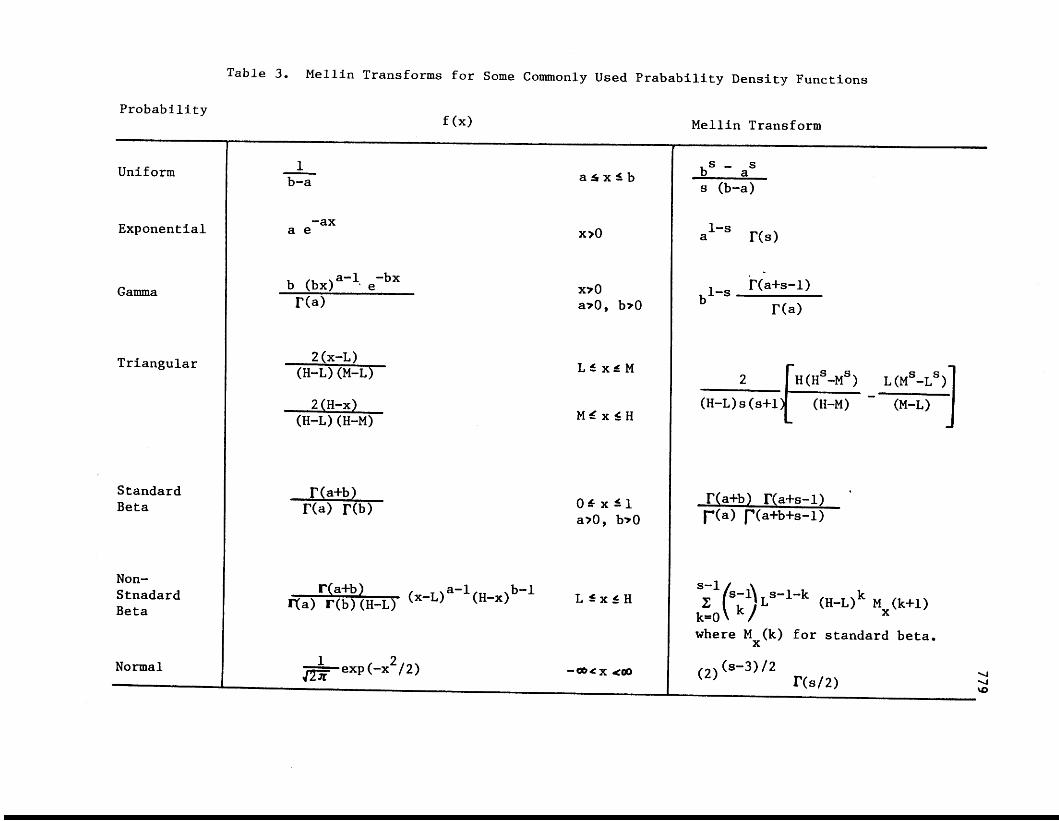
Table 3. Mellin Transforms for Some Commonly Used Prabability Density Functions

Probability Mellin Transform

Uniform

Exponen

Gamma

ial

Triangular

Standard Beta

Non- Stnadard Beta

Normal

1 b-a -

-ax a e

2 (x-L) (H-L) (M-L)

2 ( H-X) (H-L) (H-M)

a f x S b

L C x g M

M i x S H

bs - as s (b-a)

rw 1-s a

s-1

k=O (H-L) Mx (k+l)

where M (k) for standard beta. X

780

S n

M,(s)

S B

M, (s)

S

M,, ( s )

S

Q M J s )

S L

M, ( s )

= E(T~)

Table 5. Computations of the Numerical Example In Assessing The Uncertainty of the Travel Time.

Order of Moment of The Travel Time

1 2 3 4

1.6 2.2 2.8 3.4

1.52E-1 2.323-2 3.55E-3 5.48E-4

1.4 1.8 2.2 2.6

8.32E+O 6 . 93E+1 5.77E+2 4 . 81E+3 0.7 0.4 0.1 -0.2

1 . 09E+1 1.19E+2 1.31E+3 1.43E+4

0.6 0.2 -0.2 -0.6

2.51E-2 6.31E-4 1.59E-5 3 . 993-7 2.0 3.0 4.0 5.0

1 . 00E+2 l000E+4 1.00E+6 1 . 00E+8 16.36 2 . 70E+2 4.473+3 7.47E+4

1.39 I -0.48 I 9.00

FOSM I 16.54 I 1.34 1 -0.30 I

Table 6. The 90% and 95% Confidence Intervals of the Travel Time ( in Days ) .

Distln

Normal

Log-normal

Fisher- Cornish

Pearson

Confidence Intervals 1

90% 95%

(14.08,18.64)

(14.18,18.74)

(14.06,18.28)

(14.11,18.44)

(13.64,19.08)

(13.81,19.25)

(12 . 80,19.30) (13.45,18.97)

1.0

0.8

0.6

0.4

0.2

n n

" 'YO 11 12 13 1 4 15 16 18

TRAVEL TIME (in DAYS)

Figure 1. Comparison of the Cumulative Distribution Functions of the Travel Time