NUMERICAL MODELING OF MULTIPHASE FLOW IN POROUS MEDIA

Myron B. Allen July 1985

Symposium Paper WWRC - 8 5 - 22

In

Proceedings

NATO Advanced Study Institute on Fundamentals

of Transport, Phenomena in Porous Media,

Newark, Delaware

July 14-23, 1985

Myron B. Allen Department of Mathematics University of Wyoming

Laramie, Wyoming

Proceedings, NATO Advanced Study Institute on Fundamentals of Transport Phenomena in Porous Media, J. Bear and M. Y. Corapcioglu, eds., July 14 - 23, 1985, Newark, Delaware, Martinus Nijhoff, publishers.

NUMERICAL MODELING OF MULTIPHASE FLOW IN POROUS MEDIA

Myron B. Allen I11 Department of Mathematics University of Wyoming Laramie, Wyoming 82071, U.S.A.

ABSTRACT The simultaneous flow of immiscible fluids in porous media occurs in a

wide variety of applications. The equations governing these flows are inher- ently nonlinear, and the geometries and material properties characterizing many problems in petroleum and groundwater engineering can be quite irreg- ular. As a result, numerical simulation often offers the only viable approach to the mathematical modeling of multiphase flows. This paper provides an overview of the types of models that are used in this field and highlights

-some of the numerical techniques that have appeared recently. The exposi- tion includes discussions of multiphase, multispecies flows in which chemical transport and interphase mass transfers play important roles. The paper also examines some of the outstanding physical and mathematical problems in multiphase flow simulation. The scope of the paper is limited to isothermal flows in natural porous media; however, many of the special techniques and difficulties discussed also arise in artificial porous media and multiphase flows with thermal effects. 1. INTRODUCTION

.

1.1 Importance of MultiDhase Flow in Porous Media Multiphase flows in porous media occur in a variety of settings in applied

science. The earliest applications involving the simultaneous flow of two fluids through a porous solid appear in the soil science literature, where the flow of water in soils partly occupied by air has fundamental importance (128). This unsaturated Aow in some ways represents the simplest of multiphase flows. Yet, as we shall see, it exemplifies a fact underlying the continued growth in

research in this area: multiphase flows in porous media are inherently non- linear. Consequently, numerical simulation often furnishes the only effective strategy for understanding their behavior quantitatively.

Although the earliest studies of multiphase flows in porous media concern unsaturated flows, the most concentrated research in this field over the past four decades has focused on flows in underground petroleum reservoirs. Natu- ral oil deposits almost always contain connate water and occasionally contain free natural gas as well. The simultaneous flow of oil, gas, and water in porous media therefore affects practically every aspect of the reservoir engineer’s job of optimizing the recovery of hydrocarbons. Here, again, the physics of mul- tiphase fluid flows give rise to nonlinear governing equations. The difficulty imposed by the nonlinearities along with the irregular geometries and tran- sient behavior associated with typical oil reservoirs make numerical simulation an essential tool in petroleum engineering. The advent of various enhanced oil recovery technologies has added to this field further levels of complexity and hence an even greater degree of reliance on numerical methods.

Most recently, multiphase flows have generated serious interest among hydrologists concerned with groundwater quality. There is growing aware- ness that many contaminants threatening our groundwater resources enter water-bearing rock formations as separate, nonaqueous phases. These oily liquids may come from underground or near-surface storage facilities, land- fills at which chemical wastes are dumped, industrial sites such as oil refineries or wood-treatment plants, or illegal waste disposal. Regardless of the source of the contaminants, our ability to understand and predict their flows under- ground is crucial to the design of sound remedial measures. This is a fairly new frontier in multiphase porous-media flows, and again the inherent com- plexity of the physics leads to governing equations for which the only practical way to produce solutions may be numerical simulation. 1.2 Scope of the Article

The purpose of this article is to review some of the more salient appli- cations of numerical simulation in multiphase porous-media flows. In light of the history and breadth of these applications, a review of this kind must choose between the impossibly ambitious goal of thoroughness and the risks of narrowness that accompany selective coverage. This article steers toward selective coverage. The aim here is to survey several multiphase flows that have attracted substantial scientific interest and to discuss a few aspects of their numerical simulation that have appeared in the recent technical liter- ature. I confess at the outset that some important multiphase flows receive no attention here at all, and, even for the flows discussed, many potentially far-reaching contributions to numerical simulation get no mention. Perhaps the references given throughout the article can compensate in part for these

shortcomings.

In particular, we shall restrict our attention here to underground flows in natural porous media. This restriction excludes many applications in chemi- cal engineering, one notable example being flows in packed beds of catalysts. Also, the article considers only isothermal flows. Therefore we do not dis- cuss steam-water flows in geothermal reservoirs or such thermal methods of enhanced oil recovery as steam injection or fireflooding. Several numerical methods also receive scant or no mention. Among these are integrated fi- nite differences, subdomain finite elements, spectral methods, and boundary- element techniques. Some of these approaches undoubtedly hold promise for future applications in multiphase flows in porous media. For the present, however, we concentrate on developments based on the trinity of more stan- dard discrete approximations: finite differences, Galerkin finite elements, and collocation.

2. BACKGROUND 2.1 Definitions

From a quantitative point of view, one of the most fruitful ways of exam- ining multiphase flows in porous media is through the framework of continuum mixture theory. In contrast to a single continuum, a mixture is a set of over- lapping continua called constituents. Any point in a mixture can in principle be the locus of material from each constituent, and each constituent possesses its own kinematic and kinetic variables such as density, velocity, stress and so forth. How one decomposes a physical mixture into constituents depends largely on one’s theoretical aims, but in analyzing porous media we commonly identify the solid matrix as one constituent and each of the fluids occupying its interstices as another.

In discussions of porous-media physics it is important to distinguish be- tween multiphase mixtures and multispecies mixtures. A mixture consists of several phases if, on a microscopic length scale comparable, say, to typical pore apertures, one observes sharp interfaces in material properties. In this sense all porous-media flows involve multiphase mixtures, owing to the dis- tinct boundary between the solid matrix and the interstitial fluids. At this boundary, density, for example, changes abruptly from its value in the solid to that in the fluid. More complicated multiphase mixtures occur, common examples being the simultaneous flows of air and water, oil and water, or oil and gas through porous rock. Here, in addition to rock-fluid interfaces, we ob- serve interfaces between the various immiscible fluids at the microscopic scale. While the detailed structures of these interfaces and the volumes they bound are inaccessible to macroscopic observation, their geometry influences the me- chanics of the mixture. This, at least intuitively, is why volume fractions play

an important role in multiphase mixture theory. The volume fraction 4, of phase a! is a dimensionless scalar function of position and time such that 0 5 5 1, and, for any spatial region R in the mixture, sR 4, dx gives the fraction of the volume of R occupied by phase a. The sum of the fluid volume fractions in a saturated solid matrix is the porosity 4.

On the other hand, there are mixtures in which no microscopic interfaces appear. Saltwater is an example. Here the constituents are ionic or chemical species, and spatial segregation of these constituents is not observable except, perhaps, at intermolecular length scales. Air is another multispecies mixture, consisting of N2, 0 2 , ( 3 0 2 , and some trace gases. Multispecies mixtures differ from multiphase mixtures in that volume fractions do not appear in the kinematics of the former.

It is possible to have multiphase, multispecies mixtures. These composi- tional flows occur in porous-media physics when there are several fluid phases, each of which comprises several chemical species. Such mixtures arise in many flows of practical interest, two important examples being multiple-contact miscible displacement in oil reservoirs and the contamination of groundwater by nonaqueous liquids. In these cases the transfer of chemical species between phases is a salient feature of the mixture mechanics. More detailed treatment of compositional flows appears later in this article.

2.2 Review of the Basic Physics

While the theory of mixtures dates at least to Eringen and Ingram (61), its foundations are still the focus of active inquiry, as reviewed by Atkin and Craine (17). Among the applications of mixture theory to multiphase mix- tures and porous media are investigations by Prbvost (124), Bowen (29,30), Passman, Nunziato, and Walsh (112), and Raats (126). The aims of the present article in this respect are much more limited in scope than those just cited. What follows is a brief review of the basic physics of multiphase flows in porous media, using the language of mixture theory as a vehicle for the development of governing equations (7).

For concreteness, assume that the mixture under investigation has three phases: rock (R) and two fluids ( N , W ) . (The extension of this exposition to mixtures with more fluid phases is straightforward.) Each phase a! has its own intrinsic mass density pa, measured in kg/m3; velocity v,, measured in m/s; and volume fraction &. From their definitions, the volume fractions clearly must obey the constraint E,cja = 1. In terms of these mechanical variables, the mass balance for any particular phase a is

where ta stands for the rate of mass transfer into phase a from other phases. To guarantee mass conservation in the overall mixture, the reaction rates must obey the constraint c, t, = 0.

We can rewrite Eq. (2.1) in a more common form by noting that the porosity is 4 = 1 - #R and defining the fluid saturations SN = 4N/4, Sw = 4w14. Thus

d at -“1- 4)PRI + v [(I - 4)PRVRI = + R

for the rock phase, and

a = N , W , d at - (W*Pa) + v (4S*PaV*) = rot ,

for the fluids. Each phase also obeys a momentum balance. In its primitive form this

equation relates the phase’s inertia to its stress t,, body forces b,, and rate m, of momentum exchange from other phases. Thus,

&pa (2 + v, V v , ) - V ta - dapaba = mar - vara

If we assume that the rock phase is chemicalIy inert, so t~ = 0, and fix a coordinate system in which VR = 0, then the momentum balance for rock reduces to

V * t ~ - ~ R P R ~ R = m~ Let us assume that each fluid is Newtonian and that momentum trans-

fer via shear stresses within the fluid is negligible compared with momentum exchange to the rock matrix. In this case t, = -pa l , where pa is the me- chanicslpressure in fluid Q and 1 is the unit isotropic tensor. If gravity is the only body force acting on fluid phase a, then &ba = g V Z , where g stands for the magnitude of gravitational acceleration and 2 represents depth below some datum. For the momentum exchange terms, the assumption common to most theories of porous media is that momemtum losses to the solid matrix take the form of possibly anisotropic Stokes drags,

barna = ~ ( V R -Yp> = -4v,

where A, is a tensor called the mobility of phase a. If we assume further that the inertial effects in the fluid are negligible compared with rock-fluid interactions and that there is no interphase mass transfer, then Eq. (2.3) yields

which is familiar as Darcy’s law. Clearly, the mobility A, appearing in Eq. (2.4) accounts for much of the

predictive power of Darcy’s law in any particular rock-fluid system. Con- stitutive laws for mobility are largely phenomenological, the most common versions having the form A, = kkra/p,, where pa is the dynamic viscosity of fluid phase a, k is the permeability, and the relative permeability ICr, is a coefficient describing the effects of other fluids in obstructing the flow of fluid

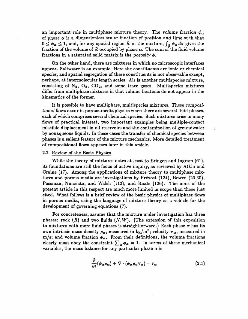
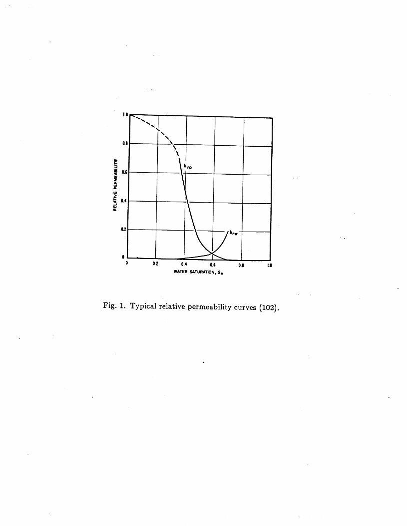
For a two-fluid system with no interphase mass transfer, the relative per- meabilities typically vary with saturation, and the curves k r N (&) , krw (Sw) look roughly like those drawn in Figure 1 (102). The vanishing-point satu- rations SN,- and Swr are called residual or irreducible saturations, and they account for the fact that, for a particular fluid to flow, it must be present at a sufficient degree of saturation to permit the formation of connected flow channels consisting of that phase. Actually, this picture of relative perme- abilities is quite simplistic. In nature relative permeabilities often exhibit significant hysteresis, and the verification of the relative-permeability model in the presence of three or more fluid phases (92,144,101) or compositional effects (22,14) is still not clear.

Eq. (2.4) allows each fluid phase to have its own pressure at any point in the reservoir. These pressure differences indeed occur in nature. At the microscopic scale the effects of interfacial tension and pore geometry on the curvatures of fluid-fluid interfaces lead to capillary effects. Leverett (91) uses the classical thermodynamics of Gibbs (75) to describe these effects, while more recent works such as those of Morrow (103) and Davis and Scriven (51) draw connections with microscopic effects and molecular theories of interfacial tension. These theories imply that, at a macroscopic scale, there will be a pressure difference, or capillary pressure, between any two fluid phases in a porous medium. In two-phase systems, for example, there is a single capillary pressure PCNW = PN - pw. In simple models PCNW is a function of saturation; however, in actual flows the capillary pressure exhibits rather pronounced hysteresis (103,82,134) and dependence on fluid composition (42).

Given velocity field equations such as Eq. (2.4), we can expand the mass balances for the fluid phases to get flow equations for each fluid. Using the cus- tomary decomposition of the mobility A, and directly substituting Eq. (2.4) into Eq. (2.2) yields, for a two-phase system,

a.

. .

\ \

\

A t

i

f

z W Q

W >

w a

.. z, k ro

1.

a

O.(

0.4

0.2

0

0 0.2 0.4 ‘Qkrw 0. L 0.1 I. 0 WATER SATURATK)N, Sw

Fig. 1. Typical relative permeability curves (102).

Flow equations for systems having more fluid phases will be similar, except that if P phases coexist, then P - 1 independent capillary pressure functions will appear in the system.

2.3 Early Investigations

The picture of multiphase flows in porous media outlined above evolved over several decades beginning in the 1930’s. The use of an extended ver- sion of the single-phase form of Darcy’s law in multiphase flows appears to have begun with Richards (128) in his work on unsaturated flows in the soil physics literature. The explicit use of a separate velocity field equation for each fluid began in the petroleum industry. Here the pioneering work of Muskat et al. (104), Wykoff and Botset (161), Buckley and Leverett ( 3 4 , Fatt and Dykstra (68), and Welge (159), among others, promoted the widespread acceptance of Darcy’s equation altered by the incorporation of relative per- meabilities. Today this model is the one most widely used in the prediction of multiphase flows in porous media.

Despite its broad appeal in applications, the multiphase version of Darcy’s law has some limitations. Relative permeabilities are not strictly functions of saturation, the most glaring violation being the phenomenon of hysteresis or dependence on saturation history. Such microscopic phenomena as gas slippage at the solid walls, turbulence, and adsorption can also inval- idate the Darcy model in certain flows (33). These limitations are worthy of consideration in the application of the multiphase Darcy law to any new rock-fluid system.

.

3. TWO-PHASE FLOWS

The simplest multiphase flows in porous media are those in which two fluids flow simultaneously but do not exchange mass or react with the solid matrix. While many flows of practical interest exhibit more complex physics, two-phase flows have drawn attention in many applications. Among these are unsaturated groundwater flows, salt-water intrusion in coastal aquifers, and the Buckley-Leverett problem in petroleum engineering.

-

3.1 Unsaturated Groundwater Flow

In typical soil profiles some distance separates the earth’s surface from the water table, which is the upper limit of completely water-saturated soil. In this intervening zone the water saturation varies between 0 and 1, the rest of the pore space normally being occupied by air. Water flow in this unsaturated zone is complicated by the fact water depends on its water saturation. Let us governing equation and examine some of the arise in its solution.

that the soil’s permeability to derive the common form of the computational- difficulties that

Most formulations of unsaturated flow rest on the assumption that the motion of air has negligible effect on the motion of water. Therefore one usually neglects the flow equation for air, assuming that the air pressure equals the constant atmospheric pressure at the surface, that is, PA = patm. Then we can define the pressure head in the water by 91, = (pw - p A ) / ( p w g ) , having the dimensions of length and being negative in the unsaturated zone where SW < 1. Also, instead of saturation, soil physicists typically refer to the soil’s moisture content, defined by 0 = #SW. In terms of these new variables the capillary pressure relationship for the air-water system becomes 91, = +(@) or, provided rl) is an invertible function, 0 = O($). From Eq. (2.5b), the flow equation for water thus transforms to

where K = pwgkkrw/pw is the hydraulic conductivity of the soil. Notice that K is a function of t,b, since relative permeability depends on saturation, which varies with 91, according to the capillarity relationship.

In many unsaturated flows the compressibility effects in water are small, so that time derivatives and spatial gradients of pw may be neglected. If this approximation holds, then the flow equation reduces to

To get an equation in which rl) is the principal unknown, we simply use the chain rule to expand the time derivative on the left, giving

where C($) = dO/d$ is the specific moisture capacity. If the flow is essen- tially one-dimensional in the vertical direction, then this equation collapses to

which is Richards’ equation (128). Several investigators in hydrology have examined the unsaturated flow

equation from analytic viewpoints. Philip (119) gives one of the earliest the- oretical treatments of Richards’ equation, proposing asymptotic solutions for a nonlinear problem. The equation has also attracted interest in the applied mathematics community, including investigations by Aronson (16), Peletier

(116), and Nakano (105). Aronson (16), for example, observes that, while the classical linear heat equation admits solutions in which disturbances propa- gate with infinite speeds, the nonlinear Eq. (3.2) may propagate disturbances with only finite speed. This implies that a moving interface, or wetting front, can form between the downward-moving zone of high moisture content 0 and the zone yet uncontacted by the wave of infiltrating water. Under certain initial conditions this moving boundary can exhibit steep spatial gradients in 0 and consequently in q!~. The resulting sharp fronts pose considerable difficulty in the construction of numerical schemes, since the discrete approx- imations used typically have lowest-order error terms that increase with the norm of the solution’s gradient. We shall discuss this difficulty in more detail in Section 6.

Numerical work by a variety of investigators has corroborated the ex- istence of wetting fronts. Much of this work appeared during the 1970’s, and it includes articles by Bresler (33), Neuman (107), Reeves and Duguid (127), Narasimhan and Witherspoon (106), and Segol (136). Van Genuchten (151,152) presents solution schemes for the one- and two-dimensional versions of Richards’ equation using both finite differences and finite-element Galerkin methods employing Hermite cubic basis functions. His work furnishes a good comparison of the finite-difference and finite-element approaches to the ap- proximation of wetting fronts.

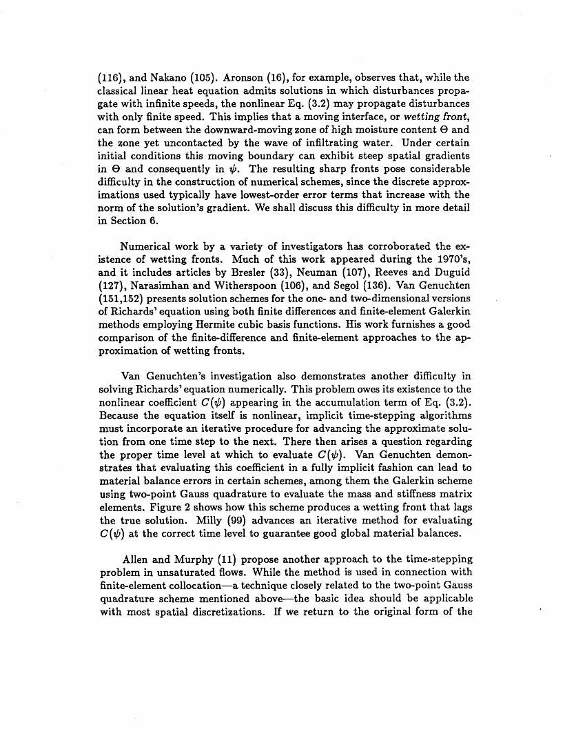
Van Genuchten’s investigation also demonstrates another difficulty in solving Richards’ equation numerically. This problem owes its existence to the nonlinear coefficient C($) appearing in the accumulation term of Eq. (3.2). Because the equation itself is nonlinear, implicit time-stepping algorithms must incorporate an iterative procedure for advancing the approximate solu- tion from one time step to the next. There then arises a question regarding the proper time level at which to evaluate C(+). Van Genuchten demon- strates that evaluating this coefficient in a fully implicit fashion can lead to material balance errors in certain schemes, among them the Galerkin scheme using two-point Gauss quadrature to evaluate the mass and stiffness matrix elements. Figure 2 shows how this scheme produces a wetting front that lags the true solution. Milly (99) advances an iterative method for evaluating C($) at the correct time level to guarantee good global material balances.

Allen and Murphy (11) propose another approach to the time-stepping problem in unsaturated flows. While the method is used in connection with finite-element collocation-a technique closely related to the two-point Gauss quadrature scheme mentioned above-the basic idea should be applicable with most spatial discretizations. If we return to the original form of the

MOISTURE CONTENT (cm3/cm3)

E 0 Y

I

I

Fig. 2. Solutions to the unsaturated flow equation using vari- ous finite-element Galerkin schemes (151).

accumulation term, Eq.

One can circumvent the

(3.2) becomes

ao at = dz [ K ($) (g + I)]

difficulties encountered in solving an equation in both 0 and + by properly formulating an iterative procedure. Let us approximate the time derivative using implicit finite differences:

We can linearize the flux terms in this approximation by establishing an iterative scheme in which +n+lsm represents the value of $ at the most recent known iteration level and $n+lsm+l = $n+lsm + 6$n+1'm+1 represents the value at the sought iterative level:

This expression allows the nonlinear coefficient K(yP+l) to lag by an itera- .

tion. In the accumulation term we also lag @($n+l), but in addition we linearly

project forward to the next iterative level using the Newton-like extrapolation

Here, recall that C($) = &/ti$. The value +n of pressure head at the old time level represents the value furnished by the iterative scheme after con- vergence, which a computer code can test using either of two criteria. First, one can check whether the iterative increment 6$n+1sm+1 is small enough in magnitude or norm to warrant stopping the iteration. Second, one can observe that collecting the terms involving the unknown 6$n+1sm+1 on the left and ignoring truncation error leaves the known quantity

acting as a right-hand side in the linearization. This quantity is precisely the residual to the flow equation at the rn-th iteration. Whenever IIRn+lsrnII is small in some appropriate norm, the resulting increment 6+n+1*rn+1 will

be small and, more to the point, we shall have solved the time-differenced equation to within a very small error.

It is easy to see why such a scheme conserves mass, at least to within lim- its imposed by the iterative convergence criteria. If we integrate the residual Rn+'sm(z) over the spatial domain St of the problem, we find

If the integral on the right were zero, this equation would be precisely the global mass balance for vertical unsaturated flow. Thus by iterating until IIRn+'~mll is small, we implicitly enforce the global mass balance to a desired level of accuracy. 3.2 Saltwater Intrusion

In coastal aquifers both fresh water and salt water are usually present. Being denser, the salt water underlies the fresh water, the latter forming a lens whose shape and thickness may vary with changes in pumping and recharge. Figure 3 depicts a typical coastal aquifer in cross-section. When the upper portion of the aquifer acts as a source of fresh water, it becomes important to design pumping and recharge strategies that prevent the flow of salt water into production wells.

Strictly speaking, salt water and fresh water are not separate phases. In fact they are completely miscible as fluids, and in a coastal aquifer there exists a zone lying between the two fluids in which salt concentration varies continuously. To be rigorously faithful to the physics of the problem, then, one would solve a single-phase flow equation coupled with a transport equation for salt. Indeed, one of the earliest numerical treatments of saltwater intrusion used just this approach (120). Nevertheless, the transition zone between salt and fresh water is often quite narrow in comparison with the overall thickness of the aquifer, and for computational purposes we may consider it to be a sharp interface. Such a sharp-interface approximation serves as justification for treating saltwater intrusion into coastal aquifers as a multiphase flow.

Let us consider the problem of modeling the areal movement of salt and fresh water. To get vertically averaged flow equations, we first write the equations in terms of hydraulic heads, defined in the fresh water (8') and salt water (S) as follows:

+ z , a = F or S ,

where pref is some reference value of pressure, and p , ( p ) gives the functional dependence of density on pressure. Then, after an application of the chain rule to the accumulation terms, each of equations (2.5) assumes the form

where K, = p,gkkra/pa is the hydraulic conductivity of fluid a and S,,,, = p,g[d4/dp,+ ( 4 / p a ) d p a / d p , ] is the specific storage of fluid a. For simplicity, let us assume that the rock matrix is isotropic, so that K, effectively acts as a scalar coefficient.

Next we average the flow equations (3.3) vertically by integrating with respect to z between the lower and upper limits of each zone, using Leibnitz's rule (84). For the freshwater zone, this gives (see Figure 3)

Here V = (a/&, a/ay) in Cartesian coordinates; e, signifies the unit vector in the z-direction; TF = K F ~ F ; CF = s , , F e F + s y ; and h = t i1 ${ h F d z is the vertically averaged freshwater head. The vector vc represents the velocity of the freshwater-saltwater interface; v a is the velocity of the free surface z = c, and s y is the specific yield, defined as the rate of change in storage with respect to changes in the free surface level.

In the absence of mass transfer between salt water and fresh water, a material point initially on the interface C will stay there. Since C is the locus of points where z - b = 0, this free surface condition takes the form

Multiplying this equation by q5 and subtracting from the vertically averaged equation above yields

where

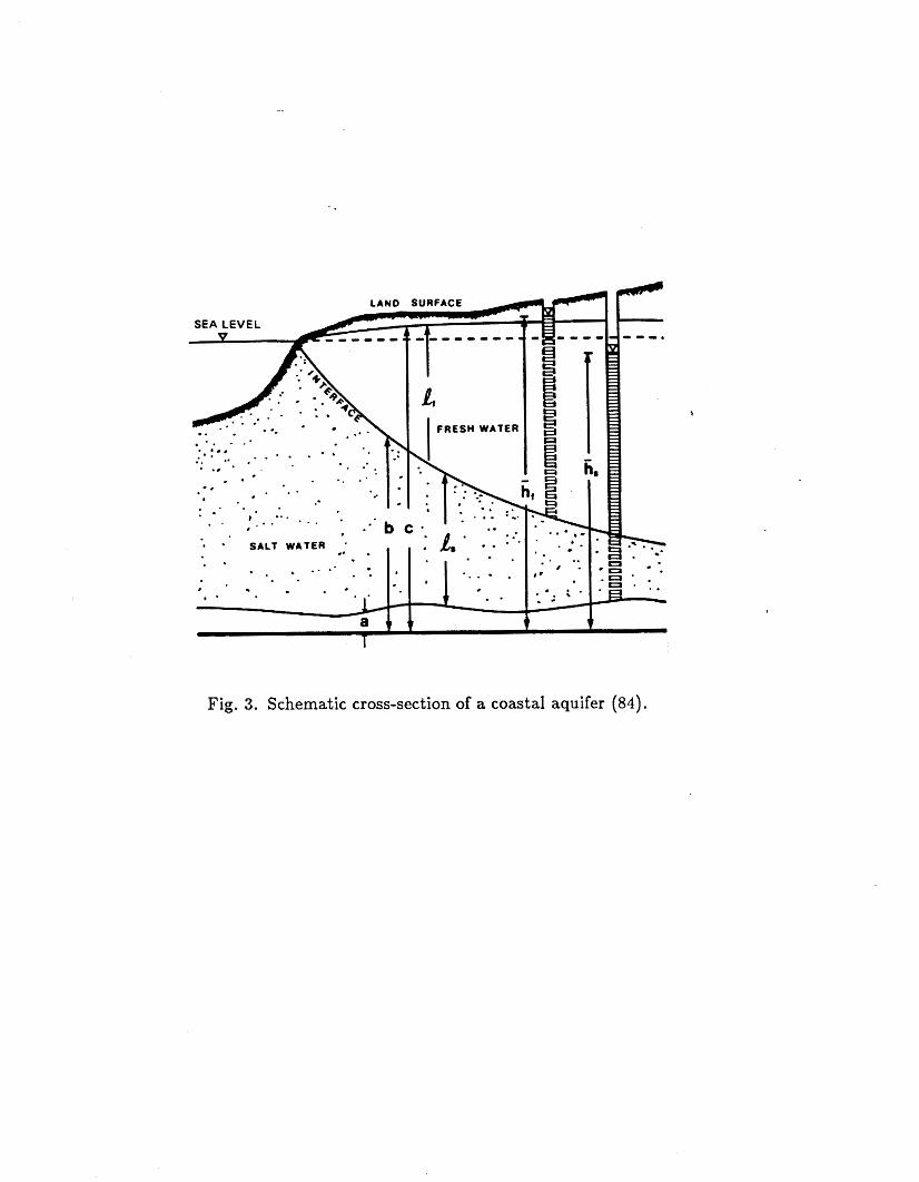
Fig. 3. Schematic cross-section of a coastal aquifer (84).

is the effective rate of withdrawal from the freshwater zone, and

QF I a=b = -(VF - 4vE) lz=b (eZ - Vb) is the effective rate of exchange of freshwater across the interface C, which we have assumed to be zero.

A similar development for salt water leads to the vertically averaged flow equation

Here TS = Ksts and Cs = S,,&. The sink terms in this equation are

which represents the effective rate of withdrawal from the saltwater zone, and

which gives the effective rate of saltwater leakage into the lower confining layer, whose depth is fixed.

To solve this system we need an equation relating &F and 5s. In this case, since the two fluids are miscible at the microscopic scale, there will be no head difference between the fluids where they are in contact. Thus the .

head is continuous across the interface C: h~ = hs at z = b. As Huyakorn and Pinder (84) show, this condition allows us to solve for db/at in terms of heads:

where p z = p C l / ( p s - p ~ ) . Combining Eq. (3.6) with Eqs. (3.4) and (3.5) yields the coupled system of flow equations

Let us examine the approximate numerical solution to Eq. (3.7) using finite-element Galerkin methods. In these methods we replace the unknown functions 6~ (x, t ) and hs (x , t ) by trial functions

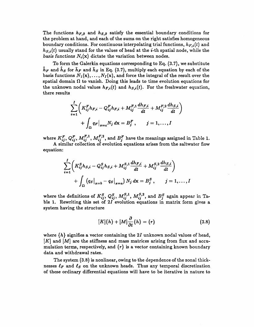
The functions h ~ , a and hs,a satisfy the essential boundary conditions for the problem at hand, and each of the sums on the right satisfies homogeneous boundary conditions. For continuous interpolating trial functions, hF,; (t) and hs,i(t) usually stand for the values of head at the i-th spatial node, while the basis functions Ni ( x ) dictate the variation between nodes.

To form the Galerkin equations corresponding to Eq. (3.7), we substitute f i , and fi, for LF and Es in Eq. (3.7), multiply each equation by each of the basis functions N1 (x), . . . , NI (x), and force the integral of the result over the spatial domain fl to vanish. Doing this leads to time evolution equations for the unknown nodal values hF,i(t) and hs,;(t) . For the freshwater equation, there results

a

where K;,. QZ, M:’, M Z 2 , and B r have the meanings assigned in Table 1. A similar collection of evolution equations arises from the saltwater flow

equation:

where the definitions of KG, QG, M;,’, M:32, and Bf again appear in Ta- ble 1. Rewriting this set of 2 1 evolution equations in matrix form gives a system having the structure

a

where {h} signifies a vector containing the 2 1 unknown nodal values of head, [K] and [MI are the stiffness and mass matrices arising from flux and accu- mulation terms, respectively, and { r } is a vector containing known boundary data and withdrawal rates.

The system (3.8) is nonlinear, owing to the dependence of the zonal thick- nesses & and ts on the unknown heads. Thus any temporal discretization of these ordinary differential equations will have to be iterative in nature to

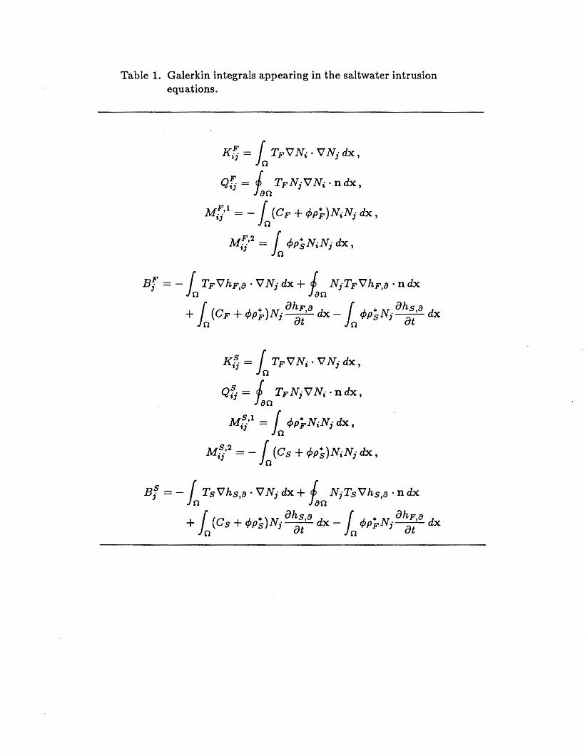
Table 1. Galerkin integrals appearing in the saltwater intrusion equations.

guarantee consistency between the numerical solution and the flow coefficients at each time level. Pinder and Page (121) advance one such iterative scheme.

The saltwater interface problem exhibits a peculiar computational dif- ficulty associated with the saltwater-freshwater interface C. This problem manifests itself as the saltwater wedge retreats or advances. Under these cir- cumstances the intersection of C with the lower confining layer, called the saltwater toe, moves horizontally. This moving boundary allows for the pos- sibility that the interface may not exist at some areal locations, and at these locations the free surface condition becomes degenerate (97). To accommo- date this degeneracy, it becomes necessary to track the moving boundary as the flow calculations proceed.

Shamir and Dagan (139) present a finite-difference algorithm for tracking the saltwater toe in a vertically integrated, immiscible setting. By examining a one-dimensional flow, they develop a scheme for regenerating the spatial grid to guarantee that the toe lies on a computational node. Thus on the ocean side of the separating node they solve the simultaneous flow equations for saltwater and freshwater heads, while on the inland side they solve the equation €or freshwater head only. This approach obviously involves a great deal of computational complexity in two or three dimensions, since it requires the construction of multidimensional moving finite-difference grids. How- ever, an analogous idea for finite-element grids in two dimensions has proved promising (55).

In another approach, SQ da Costa and Wilson (131) use a fixed, two- dimensional, quadrilateral finite-element grid to model the immiscible flow equations. They devise a toe-tracking algorithm based on the Gauss points used to compute the integrals contributing to the matrix entries in Eq. (3.8). At Gauss points inland of the toe the model assigns a very small nonzero saltwater transmissibility Ts. Thus, while the saltwater wedge never actually disappears in the numerical scheme, inland of the toe the flow of salt water is negligible.

3.3 The Buckley-Leverett Problem

The Buckley-Leverett problem serves as a fairly simple model of two- phase flow in a porous medium. The problem, introduced by Buckley and Leverett (34), has particular relevance in the petroleum industry, where gas and water injection are two common techniques for displacing oil toward production wells in underground reservoirs. The simplicity of the Buckley- Leverett problem arises from three basic assumptions. First, the total flow rate of oil and displacing fluid (say water) remains constant. Second, the rock matrix and fluids are incompressible. Third, the effects of capillary pressure gradients on the flow field are negligible compared with the pressure gradients

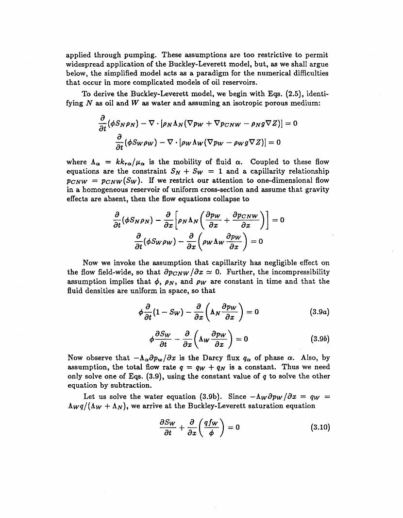
applied through pumping. These assumptions are too restrictive to permit widespread application of the Buckley-Leverett model, but, as we shall argue below, the simplified model acts as a paradigm for the numerical difficulties that occur in more complicated models of oil reservoirs.

To derive the Buckley-Leverett model, we begin with Eqs. ( 2 4 , identi- fying N as oil and W as water and assuming an isotropic porous medium:

a at -(WwPw) - v [PWAW(VPW - PWSVZ)] = 0

where A, = kkror/pa is the mobility of fluid a. Coupled to these flow equations are the constraint SN + Sw = 1 and a capillarity relationship PCNW = p c ~ w ( S w ) . If we restrict our attention to one-dimensional flow in a homogeneous reservoir of uniform cross-section and assume that gravity effects are absent, then the flow equations collapse to

dPw a a -(4Swpw) at - -(PwAwaz) dX = 0

Now we invoke the assumption that capillarity has negligible effect on the flow field-wide, so that ~ ~ C N W / ~ X = 0. Further, the incompressibility assumption implies that 4, p ~ , and pw are constant in time and that the fluid densities are uniform in space, so that

d , - , ( A w ~ ) = O asw a

(3.94

(3.9b)

Now observe that -A,ap , /ax is the Darcy flux qa of phase a. Also, by assumption, the total flow rate g = qw + q N is a constant. Thus we need only solve one of Eqs. (3.9), using the constant value of q to solve the other equation by subtract ion.

Let us solve the water equation (3.9b). Since -Awdpw/ax = qw = Awq/(Aw + AN), we arrive at the Buckley-Leverett saturation equation

(3.10)

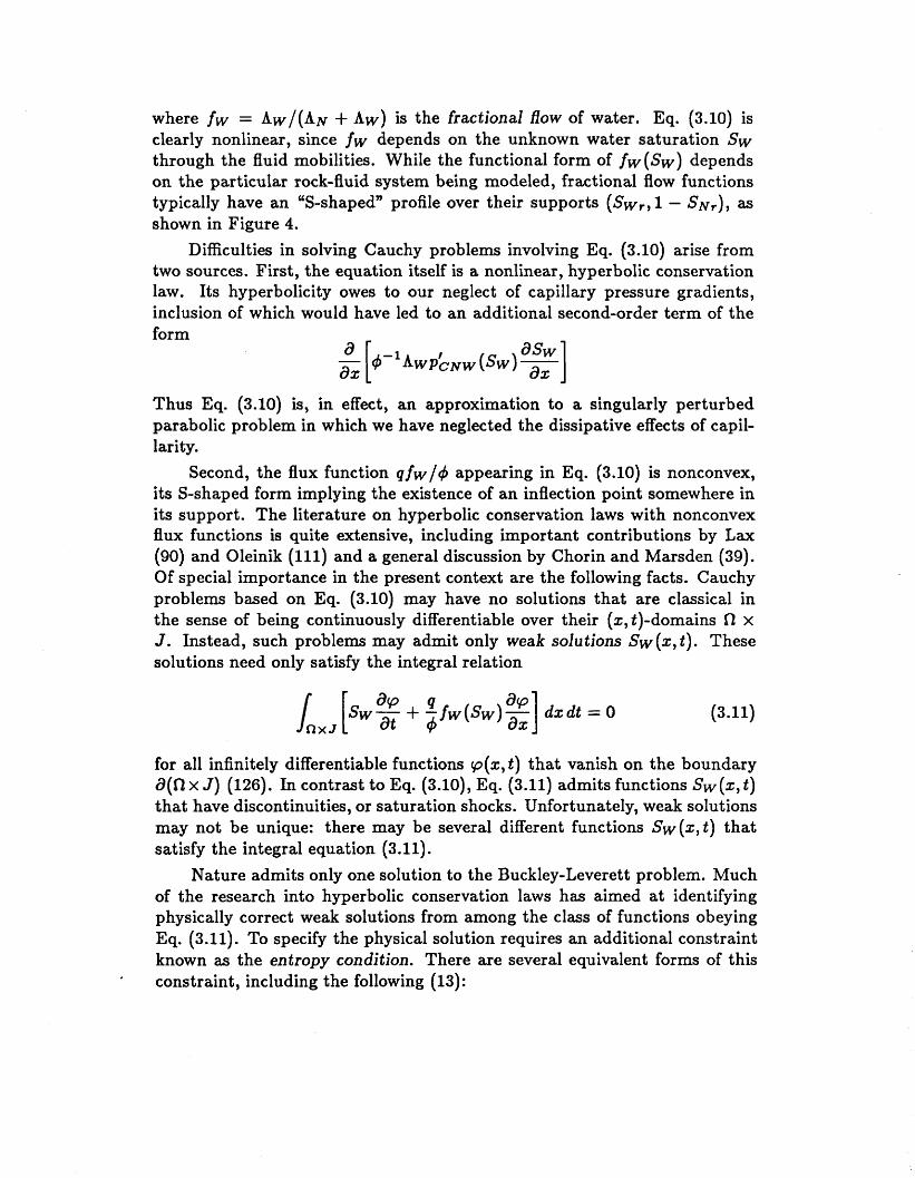
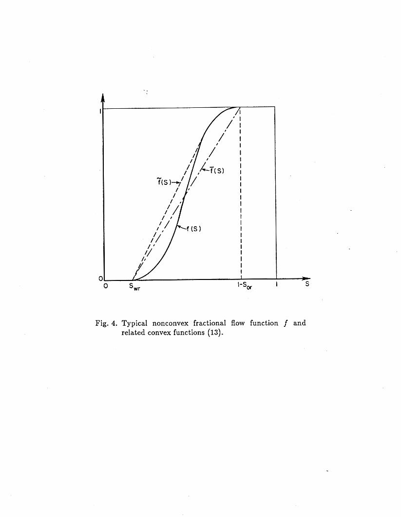
where fw = Aw/(AN + Aw) is the fractional flow of water. Eq. (3.10) is clearly nonlinear, since jw depends on the unknown water saturation SW through the fluid mobilities. While the functional form of fw(Sw) depends on the particular rock-fluid system being modeled, fractional flow functions typically have an “S-shaped” profile over their supports (Sw,,l - SN~), as shown in Figure 4.

Difficulties in solving Cauchy problems involving Eq. (3.10) arise from two sources. First, the equation itself is a nonlinear, hyperbolic conservation law. Its hyperbolicity owes to our neglect of capillary pressure gradients, inclusion of which would have led to an additional second-order term of the form

Thus Eq. (3.10) is, in effect, an approximation to a singularly perturbed parabolic problem in which we have neglected the dissipative effects of capil- larity.

Second, the flux function qfw/tj appearing in Eq. (3.10) is nonconvex, its S-shaped form implying the existence of an inflection point somewhere in its support. The literature on hyperbolic conservation laws with nonconvex flux functions is quite extensive, including important contributions by Lax (90) and Oleinik (111) and a general discussion by Chorin and Marsden (39). Of special importance in the present context are the following facts. Cauchy problems based on Eq. (3.10) may have no solutions that are classical in the sense of being continuously differentiable over their (s,t)-domains n x J . Instead, such problems may admit only weak solutions SW (2, t). These solutions need only satisfy the integral relation

1 n x J [ S w ~ + f f w ( S w ) ~ ] d ~ d t = O (3.11)

for all infinitely differentiable functions p(z, t) that vanish on the boundary a(n x J ) (126). In contrast to Eq. (3.10), Eq. (3.11) admits functions S,(z,t) that have discontinuities, or saturation shocks. Unfortunately, weak solutions may not be unique: there may be several different functions Sw(z,t) that satisfy the integral equation (3.11).

Nature admits only one solution to the Buckley-Leverett problem. Much of the research into hyperbolic conservation laws has aimed at identifying physically correct weak solutions from among the class of functions obeying Eq. (3.11). To specify the physical solution requires an additional constraint known as the entropy condition. There are several equivalent forms of this constraint, including the following (13): ’

C

i I I I I I I I I I I I I I I I I I I I I I I I

Fig. 4. Typical nonconvex fractional flow function f and related convex functions (13).

(9

(ii)

(iii)

The solution must depend continuously and stably on the initial data, im- plying that characteristics on both sides of a discontinuity must intersect the initial curve. The solution must be the same as that obtained using the method of characteristics with fw (SW) replaced by its convex hull. The solution must be the limit of solutions, for the same initial data, to a parabolic problem differing from the hyperbolic one by a dissipative second-order term (in this case, capillarity) of vanishing influence.

The tangent construction advanced by Welge (159) explicitly implements con- dition (ii) while, as Welge shows in his paper, the "equal-area" rule of Buckley and Leverett (34) imposes this same constraint in a slightly different fashion.

Any numerical scheme for solving the Buckley-Leverett problem, or even more complicated models of multiphase flows that are hyperbolic in character, must respect the entropy condition or else risk producing nonphysical results. Douglas et al. (57), for example, propose adding an artificial capillarity to the Buckley-Leverett equation to force convergence to the correct physical solution. An equivalent effect can be achieved by using certain numerical approximations whose lowest-order error terms mimic the desired dissipative phenomena (8). This tactic is perhaps easiest to see in finite-difference ap- proximations. Here, an upstream-biased difference analog of the flux term d f l a x gives

Since f'(S) > 0 over the support of f, the lowest-order error term acts like the capillarity term neglected in Eq. (3.10) while vanishing linearly its Ax --+ 0. Thus upstream weighting imposes a numerical version of condition (iii) while maintaining consistency in the numerical approximation.

Several investigators have examined upstream-weighted finite-element methods for the Buckley-Leverett problem. Mercer and Faust (96) and Huyakorn and Pinder (83), for example, discuss upstream-weighted Galerkin' techniques. Shapiro and Pinder (140) advance a finite-element collocation scheme for the Buckley-Leverett problem using asymmetric basis functions.

Allen and Pinder (12,13) introduce a collocation scheme for the same problem in which upstream biasing of the collocation points leads to the appropriate numerical version of condition we begin with a continuously differentiable

I

(ii). To implement this method, trial function for saturation:

i=O

where the basis functions Ho, i (z ) , HI,&) are piecewise Hermite cubic poly- nomials ( 5 ) . S$), S#) are the unknown nodal values of Sw and dSw/az , respectively. One can similarly represent the nonlinear flux function f w :

In the standard collocation we derive ordinary differential equations for the unknown values Si, Si, by setting

at enough points Zk in the spatial unknown. Douglas and Dupont (58)

domain to give one equation for each show that, on a uniform partition zo <

< ZI = z o + IAz, one can achieve 0 (AS*) accuracy in parabolic problems by choosing the Gauss points zi + A2/2 k Ax/&, i = 1, . , I - 1, as the collocation points. As Allen and Pinder (13) demonstrate, however, this highly accurate scheme violates the entropy condition in Eq. (3.10). One can force convergence to the correct solution by evaluating the flux term at collocation points upstream of the Gauss points, as in the equation

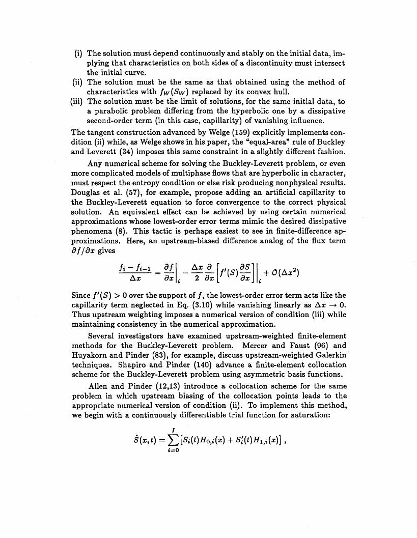
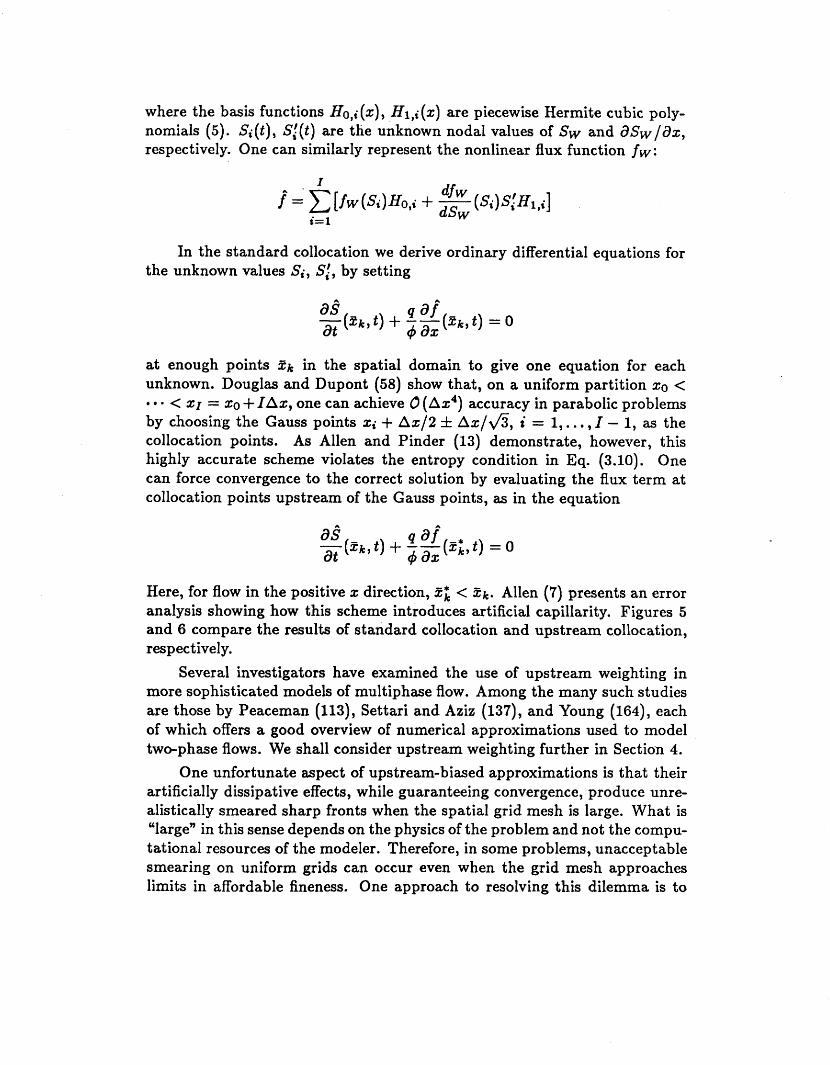
Here, for flow in the positive z direction, 3; < zk. Allen (7) presents an error analysis showing how this scheme introduces artificial capillarity. Figures 5 and 6 compare the results of standard collocation and upstream collocation, respectively.

Several investigators have examined the use of upstream weighting in more sophisticated models of multiphase flow. Among the many such studies are those by Peaceman (113), Settari and Aziz (137), and Young (164), each of which offers a good overview of numerical approximations used to model two-phase flows. We shall consider upstream weighting further in Sectiofi 4.

One unfortunate aspect of upstream-biased approximations is that their artificially dissipative effects, while guaranteeing convergence, produce unre- alistically smeared sharp fronts when the spatial grid mesh is large. What is "large" in this sense depends on the physics of the problem and not the compu- tational resources of the modeler. Therefore, in some problems, unacceptable smearing on uniform grids can occur even when the grid mesh approaches limits in affordable fineness. One approach to resolving this dilemma is to

6)

(ii)

(iii)

The solution must depend continuously and stably on the initial data, im- plying that characteristics on both sides of a discontinuity must intersect the initial curve. The solution must be the same as that obtained using the method of characteristics with fw (SW) replaced by its convex hull. The solution must be the limit of solutions, for the same initial data, to a parabolic problem differing from the hyperbolic one by a dissipative second-order term (in this case, capillarity) of vanishing influence.

The tangent construction advanced by Welge (159) explicitly implements con- dition (ii) while, as Welge shows in his paper, the “equal-area” rule of Buckley and Leverett (34) imposes this same constraint in a slightly different fashion.

Any numerical scheme for solving the Buckley-Leverett problem, or even more complicated models of multiphase flows that are hyperbolic in character, must respect the entropy condition or else risk producing nonphysical results. Douglas et al. (57), for example, propose adding an artificial capillarity to the Buckley-Leverett equation to force convergence to the correct physical solution. An equivalent effect can be achieved by using certain numerical approximations whose lowest-order error terms mimic the desired dissipative phenomena (8). This tactic is perhaps easiest to see in finite-difference ap- proximations. Here, an upstream-biased difference analog of the flux term af/ax gives

Since f‘(S) > 0 over the support of f , the lowest-order error term acts like the capillarity term neglected in Eq. (3.10) while vanishing linearly as A z + 0. Thus upstream weighting imposes a numerical version of condition (iii) while maintaining consistency in the numerical approximation.

Several investigators have examined upstream-weighted finite-element methods for the Buckley-Leverett problem. Mercer and Faust (96) and Huyakorn and Pinder (83), for example, discuss upstream-weighted Galerkin techniques. Shapiro and Pinder (140) advance a finite-element collocation scheme for the Buckley-Leverett problem using asymmetric basis functions.

Allen and Pinder (12,13) introduce a collocation scheme for the same problem in which upstream biasing of the collocation points leads to the appropriate numerical version of condition (ii). To implement this method, we begin with a continuously differentiable trial function for saturation:

I

i =O

where the basis functions Ho,i(z), H&) are piecewise Hermite cubic poly- nomials ( 5 ) . S i ( t ) , S#) are the unknown nodal values of SW and a&/&, respectively. One can similarly represent the nonlinear flux function fw :

I .1

In the standard collocation we derive ordinary differential equations for the unknown values Si, Sl, by setting

at enough points Z k in the spatial unknown. Douglas and Dupont (58)

domain to give one equation for each show that, on a uniform partition 20 <

= < z~ = z o + IAx, one can achieve 0 (Az4) accuracy in parabolic problems by choosing the Gauss points xi + Az/2 & As/&, i = 1,. . , I - 1, as the collocation points. As Allen and Pinder (13) demonstrate, however, this highly accurate scheme violates the entropy condition in Eq. (3.10). One can force convergence to the correct solution by evaluating the flux term at collocation points upstream of the Gauss points, as in the equation

Here, for flow in the positive z direction, Z i < &. Allen (7) presents an error analysis showing how this scheme introduces artificial capillarity. Figures 5 and 6 compare the results of standard collocation and upstream collocation, respectively.

Several investigators have examined the use of upstream weighting in more sophisticated models of multiphase flow. Among the many such studies are those by Peaceman (113), Settari and Aziz (137), and Young (164), each of which offers a good overview of numerical approximations used to model two-phase flows. We shall consider upstream weighting further in Section 4.

One unfortunate aspect of upstream-biased approximations is that their artificially dissipative effects, while guaranteeing convergence, produce unre- alistically smeared sharp fronts when the spatial grid mesh is large. What is “large” in this sense depends on the physics of the problem and not the compu- tational resources of the modeler. Therefore, in some problems, unacceptable smearing on uniform grids can occur even when the grid mesh approaches limits in affordable fineness. One approach to resolving this dilemma is to

01

01

S 0.L

0.2

C

I I 1 1

1.c .

0.8

0.6 S

0.4

02

0

ANALYTIC SOLUTION AT t = 1500

q =2.134X Ax =5.000X10-2 At = 5.000

t =I500

I I 1 1

1 0.2 0.4 0.6 0.8 I .o X

Fig. 5. Solution to the Buckley-Leverett problem generated by orthogonal collocation with Az = 0.1 (12).

ANALYTIC SOLUTION AT t=l500 /

I\\\ t = 1500 __o_ Ax=O.IOO - Ax =0.050 - Ax = 0.025

/

C:= -2/3

__o_ Ax=O.IOO - Ax =0.050 - Ax = 0.025

Fig. 6. Solutions to the Buckley-Leverett problem generated by upstream collocation with Ax = 0.1, 0.05, 0.025

(12)

I

refine the spatial grid only in the vicinity of the steep front. Since the front itself moves as the flow progresses, such a strategy calls for self-adaptive local grid refinement, a topic discussed in Section 6. 4. FLOWS WITH INTERPHASE MASS TRANSFER

In many multiphake flows of interest in engineering the exchange of chem- ical species among the fluid phases is crucial to the behavior of the flows. Historically, concern with the compositional aspects of multiphase flows in porous media originated in the petroleum industry, where the effects of gas dissolution, retrograde condensation, and vaporization and condensation of injected gases have substantial implications in oil recovery operations. As the complexities of groundwater contamination by organic wastes become more urgent, however, interest in multiphase flows with mass transfer has spread to the hydrology community. In this section we shall focus on the more es- tablished modeling efforts in the petroleum industry, leaving discussion of the newer applications in hydrology to Section 5. 4.1 Compositional Oil Reservoir Flows

In compositional flows there are several fluid phases in which some num- ber of chemical species reside. It is therefore necessary to extend the mixture- theoretic formalism to accommodate two different categories of constituents: phases and species. A more detailed exposition of the development given be- low appears in Allen (7). For simplicity, let us assume that there are three fluid phases, namely water (W), oil (0), and gas (G) with chemical species indexed by i = 1, ... , N + 1. As before, let us label the rock phase by the index R. Conceivably, at least, each species can exist in any phase and can transfer between phases via dissolution, evaporation, condensation, and so forth, subject to thermodynamic constraints. We shall assume here that the rock is chemically inert and that there are no intraphase or stoichiometric chemical reactions, although in such applications as enhanced oil recovery by alkaline fluid injection reactions of this kind may be important.

In our new formalism, each pair (i, a), with i chosen from the species indices and a chosen from the phases, is a constituent. Thus, for example, CH4 in the gas phase is one constituent, CH4 in oil another, and n-CdHlo in oil yet another. Each constituent (&a) has its own intrinsic mass density pi", measured as mass of i per unit volume of a, and its own velocity vq. To accommodate the familiar kinematics of phases, we shall still associate with each phase a its volume fraction &, and if 4 = 1 - 4~ as before, then we define the saturation of fluid phase a as S, = &/q5. Using these basic quantities, we define the following variables:

N

pa = p r = intrinsic mass density of phase a, i= 1

w; = pg/p" = mass fraction of species i in phase a,

p = q5 Sapa = bulk density of fluids, "#R

wi = (q#/p) Sapawq = total mass fraction of species i in the fluids, a # R N

v" = ( l / p a ) pgvq = barycentric velocity i= 1

uq = vg - V" - - diffusion velocity of species

of phase a,

i in phase a.

If the index N + 1 represents the species making up the inert rock phase, then the following constraints hold:

N N

i=l i=1 a

where the index a in the second sum can represent any fluid phase, and

Each constituent (i, a) has its own mass balance, given by analogy with Eq. (2.1) as

where the exchange terms rr must obey the restriction ziz1 N EaZR r r = 0.

If we impose the further constraint that there are no intraphase chemical re- actions, then we have in addition EorfR r r = 0 for each species i = 1,. . . , N. Since phase velocities are typically more accessible to measurement than species velocities, it is convenient to rewrite the constituent mass balance

A as

where j s = q # S a p a w ~ u ~ stands for the diffusive flux of constituent ( i , ~ ) . Summing this equation over all fluid phases Q and using the restrictions gives a total mass balance for each species i :

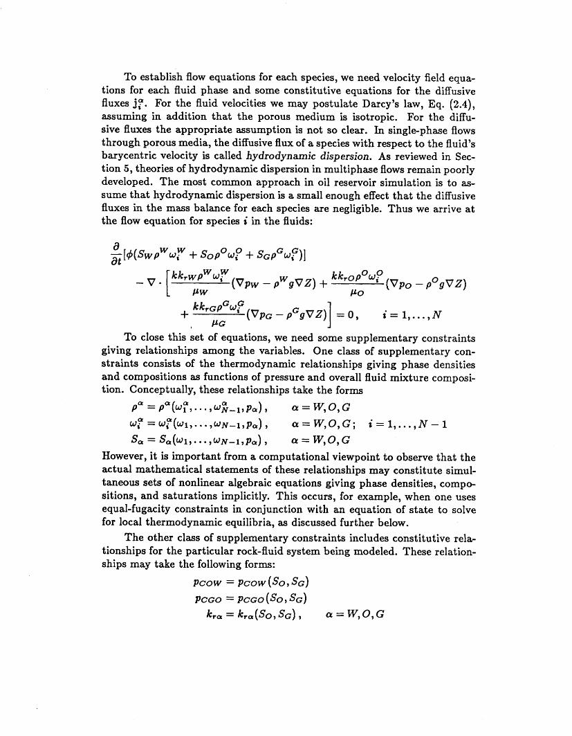
To establish flow equations for each species, we need velocity field equa- tions for each fluid phase and some constitutive equations for the diffusive fluxes j?. For the fluid velocities we may postulate Darcy’s law, Eq. (2.4), assuming in addition that the porous medium is isotropic. For the diffu- sive fluxes the appropriate assumption is not so clear. In single-phase flows through porous media, the diffusive flux of a species with respect to the fluid’s barycentric velocity is called hydrodynamic dispersion. As reviewed in Sec- tion 5 , theories of hydrodynamic dispersion in multiphase flows remain poorly developed. The most common approach in oil reservoir simulation is to as- sume that hydrodynamic dispersion is a small enough effect that the diffusive fluxes in the mass balance for each species are negligible. Thus we arrive at the flow equation for species i in the fluids:

0 0 ( V P O - POSVZ)

k k , o p wi ( V P W - PW9VZ) + PW PO

To close this set of equations, we need some supplementary constraints giving relationships among the variables. One class of supplementary con- straints consists of the thermodynamic relationships giving phase densities and compositions as functions of pressure and overall fluid mixture composi- tion. Conceptually, these relationships take the forms

Pa = P a ( W f , * . . , W E - 1 , P c r ) 9

sa = S a ( W l , * * * , W N - l , P a ) 3

a = W,O,G 09 = w 9 ( w l , . * . , W N - - l , P c r ) , Q! = W,O,G; i = 1,. . . , N - 1

a = W,O,G However, it is important from a computational viewpoint to observe that the actual mathematical statements of these relationships may constitute simul- taneous sets of nonlinear algebraic equations giving phase densities, compo- sitions, and saturations implicitly. This occurs, for example, when one uses equal-fugacity constraints in conjunction with an equation of state to solve for local thermodynamic equilibria, as discussed further below.

The other class of supplementary constraints includes constitutive rela- tionships for the particular rock-fluid system being modeled. These relation- ships may take the following forms:

Here, as mentioned in Section 2, we have greatly simplified the physics of many compositional flows by omitting possible dependencies on fluid composition through variations in interfacial tension. 4.2 Black-Oil Simulation

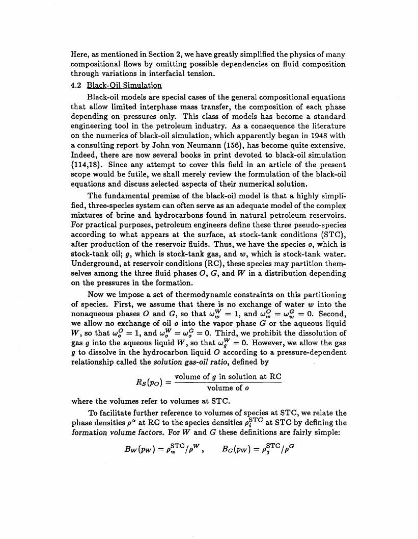
Black-oil models are special cases of the general compositional equations that allow limited interphase mass transfer, the composition of each phase depending on pressures only. This class of models has become a standard engineering tool in the petroleum industry. As a consequence the literature on the numerics of black-oil simulation, which apparently began in 1948 with a consulting report by John von Neumann (156), has become quite extensive. Indeed, there are now several books in print devoted to black-oil simulation (114,18). Since any attempt to cover this field in an article of the present scope would be futile, we shall merely review the formulation of the black-oil equations and discuss selected aspects of their numerical solution.

The fundamental premise of the black-oil model is that a highly simpli- fied, three-species system can often serve as an adequate model of the complex mixtures of brine and hydrocarbons found in natural petroleum reservoirs. For practical purposes, petroleum engineers define these three pseudo-species according to what appears at the surface, at stock-tank conditions (STC), after production of the reservoir fluids. Thus, we have the species 0, which is stock-tank oil; g, which is stock-tank gas, and w , which is stock-tank water. Underground, at reservoir conditions (RC), these species may partition them- selves among the three fluid phases 0, G, and W in a distribution depending on the pressures in the formation.

Now we impose a set of thermodynamic constraints on this partitioning of species. First, we assume that there is no exchange of water 20 into the nonaqueous phases 0 and G, so that w: = 1, and w g = 0: = 0. Second, we allow no exchange of oil o into the vapor phase G or the aqueous liquid W, so that w: = 1, and w r = w: = 0. Third, we prohibit the dissolution of gas g into the aqueous liquid W, so that w r = 0. However, we allow the gas g to dissolve in the hydrocarbon liquid 0 according to a pressure-dependent relationship called the solution gas-oil ratio, defined by

volume of g in solution at RC volume of o

&(Po) =

where the volumes refer to volumes at STC. To facilitate further reference to volumes of species at STC, we relate the

phase densities pa at RC to the species densities p f T C at STC by defining the formation volume factors. For W and G these definitions are fairly simple:

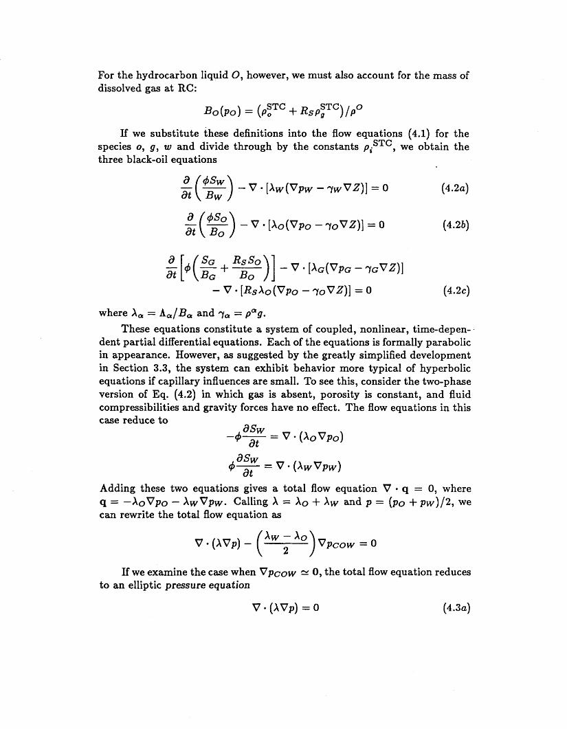
For the hydrocarbon liquid 0, however, we must also account for the mass of dissolved gas at RC:

Bo(P0) = (PfTC + RSP;TC)/po If we substitute these definitions into the flow equations (4.1) for the

species 0, g , w and divide through by the constants piSTC, we obtain the three black-oil equations

"(""w) - v [X,(Vpw - 7 w V Z ) ] = 0 dt Bw

d (*) - v [Xo(Vpo - YoVZ)] = 0 at Bo

(4.2a)

(4.2b)

- v [RsXo(Vpo - 7oVZ)I = 0 ( 4 . 2 ~ )

where A, = A,/B, and ra = pug.

These equations constitute a system of coupled, nonlinear, time-depen- dent partial differential equations. Each of the equations is formally parabolic in appearance. However, as suggested by the greatly simplified development in Section 3.3, the system can exhibit behavior more typical of hyperbolic equations if capillary influences are small. To see this, consider the two-phase version of Eq. (4.2) in which gas is absent, porosity is constant, and fluid compressibilities and gravity forces have no effect. The flow equations in this case reduce to

Adding these two equations gives a total flow equation V q = 0, where q = -XoVpo - XwVpw. Calling X = XO + X W and p = (PO + p w ) / 2 , we can rewrite the total flow equation as

Xw - A 0 (XVP) - ( )VPCOW = 0

If we examine the case when Vpcow N 0 , the total flow equation reduces to an elliptic pressure equation

v (XVp) = 0 (4.3a)

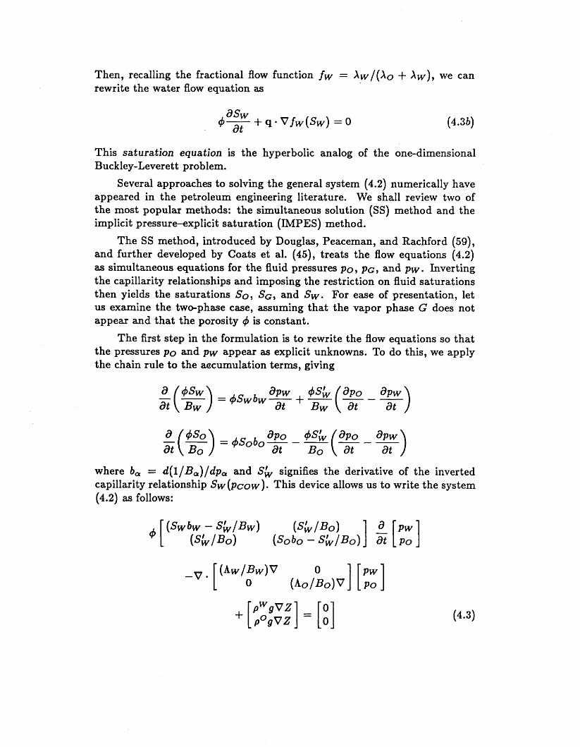
Then, recalling the fractional flow function f w = Xw/ (X , + XW), we can rewrite the water flow equation as

(4.3b)

This saturation equation is the hyperbolic analog of the one-dimensional Buckley-Leverett problem.

Several approaches to solving the general system (4.2) numerically have appeared in the petroleum engineering literature. We shall review two of the most popular methods: the simultaneous solution (SS) method and the implicit pressure-explicit saturation (IMPES) method.

The SS method, introduced by Douglas, Peaceman, and Rachford (59), and further developed by Coats et al. (45), treats the flow equations (4.2) as simultaneous equations for the fluid pressures P O , p ~ , and pw. Inverting the capillarity relationships and imposing the restriction on fluid saturations then yields the saturations SO, SG, and SW. For ease of presentation, let us examine the tw-phase case, assuming that the vapor phase G does not appear and that the porosity q5 is constant.

The first step in the formulation is to rewrite the flow equations so that the pressures p o and pw appear as explicit unknowns. To do this, we apply the chain rule to the aocumulation terms, giving

dPW 4% dPo dpw "(""w) dt Bw = +swbw- at +-(at--) BW at

where b, = d ( l / B , ) / d p , and S& signifies the derivative of the inverted capillarity relationship Sw (pcow ). This device allows us to write the system (4.2) as follows:

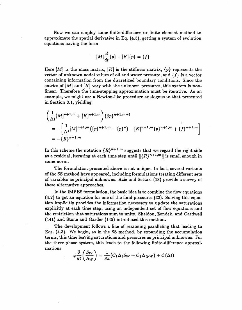
Now we can employ some finitedifference or finite element method to approximate the spatial derivative in Eq. (4.3), getting a system of evolution equations having the form

Here [ M ] is the mass matrix, [K] is the stiffness matrix, {p} represents the vector of unknown nodal values of oil and water pressure, and {f} is a vector containing information from the discretized boundary conditions. Since the entries of [MI and [K] vary with the unknown pressures, this system is non- linear. Therefore the time-stepping approximation must be iterative. As an example, we might use a Newton-like procedure analogous to that presented in Section 3.1, yielding

In this scheme the notation {R}n+lgm suggests that we regard the right side as a residual, iterating at each time step until ll(R}n+'j"ll is small enough in some norm.

The formulation presented above is not unique. In fact, several variants of the SS method have appeared, including formulations treating different sets of variables as principal unknowns. Aziz and Settari (18) provide a survey of these alternative approaches.

In the IMPES formulation, the basic idea is to combine the flow equations (4.2) to get an equation for one of the fluid pressures (32). Solving this equa- tion implicitly provides the information necessary to update the saturations explicitly at each time step, using an independent set of flow equations and the restriction that saturations sum to unity. Sheldon, Zondek, and Cardwell (141) and Stone and Garder (145) introduced this method.

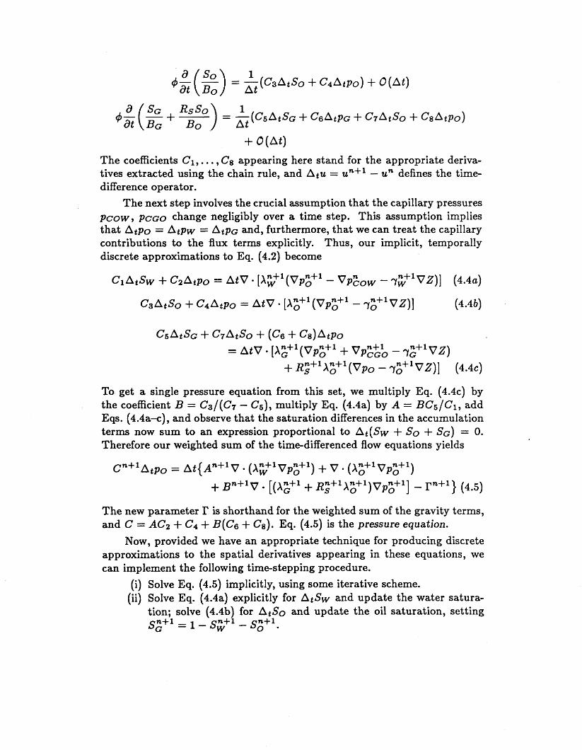
The development follows a line of reasoning paralleling that leading to Eqs. (4.3). We begin, as in the SS method, by expanding the accumulation terms, this time leaving saturations and pressures as principal unknowns. For the three-phase system, this leads to the following finite-difference approxi-

+ O(At)

The coefficients C1,. . . , C g appearing here stand for the appropriate deriva- tives extracted using the chain rule, and Atu = uh+l - un defines the time- difference operator.

The next step involves the crucial assumption that the capillary pressures pcow, PCGO change negligibly over a time step. This assumption implies that Atpo = Atpw = AtpG and, furthermore, that we can treat the capillary contributions to the flux terms explicitly. Thus, our implicit, temporally discrete approximations to Eq. (4.2) become

To get a single pressure equation from this set, we multiply Eq. (4 .4~) by the coefficient B = C3/(C7 - C5), multiply Eq. (4.4a) by A = BC&, add Eqs. (4.4a-4, and observe that the saturation differences in the accumulation terms now sum to an expression proportional to At(& + SO + S,) = 0. Therefore our weighted sum of the time-differenced flow equations yields

+ P + ~ V [(x:+l+ ~;+9;+~)vp;+l] - rn+l) (4.5)

The new parameter X' is shorthand for the weighted sum of the gravity terms, and C = AC2 + C4 + B(C6 + Cg). Eq. (4.5) is the pressure equation.

Now, provided we have an appropriate technique for producing discrete approximations to the spatial derivatives appearing in these equations, we can implement the following time-stepping procedure.

(i) Solve Eq. (4.5) implicitly, using some iterative scheme. (ii) Solve Eq. (4.4a) explicitly for AtSw and update the water satura-

tion; solve (4.4b) for Atso and update the oil saturation, setting sg+1 = 1 - s;+1- SG+?

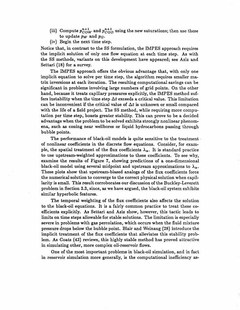
(iii) Compute to update pw and p ~ .

(iv) Begin the next time step.

and pz.+c]o using the new saturations; then use these

Notice that, in contrast to the SS formulation, the IMPES approach requires the implicit solution of only one flow equation at each time step. As with the SS methods, variants on this development have appeared; see Aziz and Settari (18) for a survey.

The IMPES approach offers the obvious advantage that, with only one implicit equation to solve per time step, the algorithm requires smaller ma- trix inversions at each iteration. The resulting computational savings can be significant in problems involving large numbers of grid points. On the other hand, because it treats capillary pressures explicitly, the IMPES method suf- fers instability when the time step At exceeds a critical value. This limitation can be inconvenient if the critical value of At is unknown or small compared with the life of a field project. The SS method, while requiring more compu- tation per time step, boasts greater stability. This can prove to be a decided advantage when the problem to be solved exhibits strongly nonlinear phenom- ena, such as coning near wellbores or liquid hydrocarbons passing through bubble points.

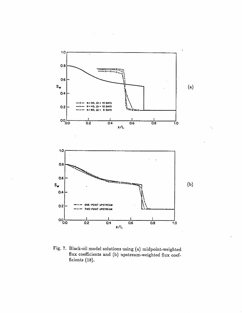
of nonlinear coefficients in the discrete flow equations. Consider, for exam- ple, the spatial treatment of the flux coefficients A,. It is standard practice to use upstream-weighted approximations to these coefficients. To see why, examine the results of Figure 7, showing predictions of a one-dimensional black-oil model using several midpoint and upstream approximations to A,. These plots show that upstream-biased analogs of the flux coefficients force the numerical solution to converge to the correct physical solution when capil- larity is small. This result corroborates our discussion of the Buckley-Leverett problem in Section 3.3, since, as we have argued, the black-oil system exhibits similar hyperbolic features.

The temporal weighting of the flux coefficients also affects the solution to the black-oil equations. It is a fairly common practice to treat these co- efficients explicitly. As Settari and Aziz show, however, this tactic leads to limits on time steps allowable for stable solutions. The limitation is especially severe in problems with gas percolation, which occurs when the fluid mixture pressure drops below the bubble point. Blair and Weinaug (28) introduce the implicit treatment of the flux coefficients that alleviates this stability prob- lem. As Coats (43) reviews, this highly stable method has proved attractive in simulating other, more complex oil-reservoir flows.

One of the most important problems in black-oil simulation, and in fact in reservoir simulation more generally, is the computational inefficiency as-

The performance of black-oil models is quite sensitive to the treatment .

0.0

0.6

S"

0.4

0.2

1 I 1 I

x/L 0.2 0.4 0.6 0.8 1 .o

- + - ONE- POINT UPSTREAM

- # - TWO-POINT UPSTREAM

Fig. 7. Black-oil model solutions using (a) midpoint-weighted flux coefficients and (b) upstream-weighted flux coef- ficients (18).

sociated with the solution of large systems of linear algebraic equations. In either the SS or the IMPES approach, the iterative time-stepping scheme calls for the solution of matrix equations at each iteration of each time step. For simulations at practical scales these calculations alone can tax the storage and CPU-time resources of the largest machines currently available. A great deal of recent research has focused on the development of fast iterative techniques for the solution of the large matrix systems arising in applications.

Among the oldest of these iterative techniques are the block-iterative methods. These methods use the blocked, sparse structure of the linear sys- tems to solve the equations iteratively, block-by-block (27). Block iterative methods, such as block-successive overrelaxation, tend to be quite sensitive to "tunable" iteration parameters such as overrelaxation coefficients.

Another fairly old class of iterative techniques consists of alternating direction methods. These methods, introduced in the context of finite dif- ferences by Peaceman and Rachford (115), Douglas and Rachford (60), and Douglas (56), reduce the computational effort in multidimensional problems by implicitly solving over one space dimension at a time. While interest in al- ternating direction techniques for finite differences has waned in recent years, interest in alternating-direction Galerkin and collocation methods has been growing; see, for example, Ewing (62) and Celia and Pinder (36).

In a different approach, Stone (143) proposes the strongly implicit proce- dure (SIP) for solving matrix equations implicitly. The idea here is to replace a matrix equation having the form [A] {p } = - {R} by an iterative scheme having the form

i- [N]){P}"+' = ( [A] + [ N ] ) { P } ~ - ([A]{p}" + {R)) By properly choosing the matrix [ N ] , one can efficiently factor ([A] + [ N ] ) into a product of sparse upper- and lower-triangular matrices. This idea gives rise to an algorithm that gives relatively rapid convergence to the solution {p} of the original equation.

Finally, much recent interest has focused on conjugate gradient methods for solving large matrix equations. These methods have their theoretical roots in the equivalence between linear systems and minimization problems for pos- itive self-adjoint matrices (95). However, the methods admit extensions to the nonself-adjoint operators that arise in fluid flow problems, especially in con- junction with such preconditioning methods as imcomplete LU factorization and nested factorization (15,110,150,122). The motivation for precondition- ing is that, for parabolic flow equations, fine spatial grids can yield iteration equations [A] {p } = -{R} in which the condition number of [A] is large. By "preconditioning" [A] with another matrix [A*]-', one can arrive at an

equivalent system [A*]- ' [A]{p} = - [A*]- ' {R}

that is better conditioned. Clever choices of [A*]-' ensure that [A*]- ' {R} will be easy to compute at each iteration, thus promoting computational efficiency. It is reasonable to expect that preconditioned conjugate-gradient methods will play a larger role in oil reservoir simulation as the technology continues to advance. 4.3 Compositional Simulation

The most amibitous applications of the equations for compositional flows arise in the simulation of enhanced oil recovery processes. Many of these processes depend for their success on the effects of interphase mass transfer on fluid flow properties. One noteworthy example of such a process is miscible gas flooding. This technology consists of injecting an originally immiscible gas, such as CO2, into an oil reservoir with the aim of developing a miscible displacement front in situ. In successful projects, miscibility develops through continuous interphase mass transfers, leading the fluid mixture toward its critical composition and hence reducing the interfacial tension between the resident oil and the displacing fluid. Compositional modeling serves as an important tool in other oil recovery problems, too, including production from gas condensate reservoirs and recovery of volatile oils.

There are several ways to classify compositional simulators. One way is to characterize the models according to their treatment of fluid-phase ther- modynamics. There are at least two fo rm in which the thermodynamic constraints mentioned in Section 4.1 can appear. The oldest form consists of tabular data for the equilibrium ratios w F / w o of species mass (or mole) fractions in the vapor and liquid hydrocarbon phases. Thus, given overall hydrocarbon pressures and compositions at a point in the reservoir, one can compute fluid saturations, densities, and compositions by performing "flash" calculations familiar to chemical engineers (109). The other form of the ther- modynamic constraints is the requirement that vapor and liquid fugacities be equal for each component: f: = fy, i = 1 , . . . , N. This approach is espe- cially attractive when used in conjunction with an equation of state such as that proposed by Peng and Robinson (117). Equation-of-state methods have the advantage of thermodynamic consistency near fluid critical points, lead- ing to calculations with better convergence properties in models of miscible gas floods. In either the equilibrium-ratio approach or the equation-of-state approach, though, the thermodynamic constraints amount to a system of non- linear algebraic equations giving fluid saturations, densities, and compositions implicit 1 y.

Another way to classify compositional models is according to the manner

'

in which they solve the flow equations (4.1). Two general schemes have ap- peared. One of these treats the flow equations sequentially, solving an overall pressure equation and then updating the remaining N - 1 composition equa- tions and the thermodynamic constraints at each time step or iteration. This approach parallels the IMPES method in black-oil simulation, and, as one might expect, it offers computational speed at the expense of some stability. The other scheme solves the entire system of flow equations and thermody- namic constraints simultaneously at each time step. This approach, analogous to the SS method of Section 4.2, leads to enormous matrix equations at each iteration. However, it enjoys greater stability than the sequential schemes. Given adequate computers, this fully implicit approach is quite attractive, since the compositional equations can exhibit behavior that is too complex to permit a priori estimates of stability constraints.

Among the simulators using sequential methods are those advanced by Roebuck et al. (130); Nolen (109); Van Quy, Corteville, and Simandoux (153); Kazemi, Vestal, and Shank (88); Nghiem, Fong, and Aziz (108); Watts (158), and Allen (6,7). Let u s examine the time-stepping structure of one such model (7), restricting attention to an oil-gas system in which gravity has no effect. Summing the flow equations over all N species gives an overall fluid mass balance

(4 -6) dP at - = v (TTVPG - TOVPCGO)

where T, = kkr,pu/pa for each fluid a and TT = TG +TO. This leaves N - 1 independent species balances

where Ti = TGW? + TOW?. We can regard Eq. (4.6) as an equation for the pressure p ~ , using Eq. (4.7) to solve for the overall species mass fractions wi . The thermodynamic constraints then give the saturation, densities, and compositions of the liquid and vapor phases.

To solve these equations sequentially, we first discretize the pressure equa- tion (4.6) in time, using the following Newton-like iterative scheme:

This scheme is similar to that used in the unsaturated flow equation of See- , we update the pressure iterate by tion 3.1. After solving for 6 p , n + l , m + l

. Then we can update each mass n+l,m n+ 1 ,m+ 1 setting p, fraction w 1 , . . . , W N - ~ using the finite difference approximation

= PG +sP, n+l,m+l

to Eq. (4.7), setting w ~ ? + ~ ~ ~ + ~ = w r + AtWl+l,m+l . This update calls for values of pn+lsrn+l, which are available from the latest iteration of Eq. (4.8) as

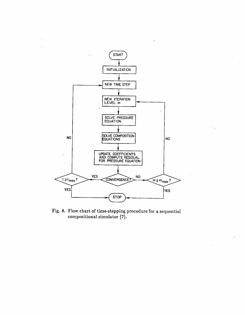
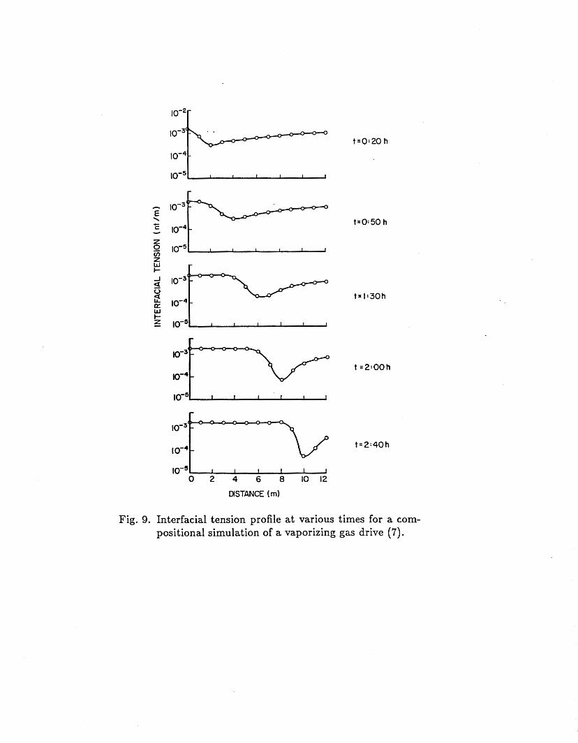
This iterative sequence requires the solution of a matrix equation only in the spatially discrete analog of Eq. (4.8), since Eq. (4.9) has an "explicit" form at each iteration. Notice that, while the scheme is not fully implicit, it calls for implicit treatment of the flux coefficients, which lends to the sta- bility of the formulation. Figure 8 shows a flow chart for the time-stepping algorithm, and Figure 9 shows a profile of vapor-liquid interfacial tensions in a simulated vaporizing gas drive (7). The wave of decreasing tensions indi- cates the development of a zone in which the fluid displacement is very nearly miscible.

With the advent of large, fast digital computers, interest has grown in the fully implicit approach to compositional simulation. Among the models based on this approach are those reported by Fussell and Fussell (72), Coats (42), Heinemann (80), and Chien, Lee and Chen (38). This class of formulations treats the discretized flow equations and thermodynamic constraints as a set of simultaneous nonlinear algebraic equations, generally using some Newton- like iterative scheme to advance between time steps. The implicit nature of the formulations leads to great stability at the expense of solving large matrix equations of the form [A]{y} = - {R} at each iteration. Moreover, the iter- ation matrix [A] typically has less sparseness than the matrices arising from sequential schemes, since simultaneous schemes account for more of the non- linear coupling between variables. Young and Stephenson (165) present one approach to mitigating this complication by evaluating the flux coefficients explicitly. As should be expected, this scheme reduces the computational effort of the fully implicit approach while sacrificing some of its stability.

There are several areas of difficulty common to practically all composi- tional simulators. One class of problems concerns the mathematical represen- tation of fluid phase behavior. Most research in compositional simulation now focuses on methods using cubic equations of state coupled with equal-fugacity constraints to represent the fluid thermodynamics. While this approach guar- antees thermodynamic consistency and therefore ensures smooth behavior of

NC

v NEW TiME STEP 1

NEW ITERATON LEVEL m

I SOLVE PRESSURE EQUATION I

EQUATIONS

AND COMPUTE RESIDUAL FOR PRESSURE EQUATION

NO

YES YES

Fig. 8. Flow chart of time-stepping procedure for a sequential compositional simulator (7).

n

E \ C c

Y

t=0:20 h

I

10-4t---- 1 0 ’ ~ 10-31

t=0:50 h

t=1:30h

t =2:00h

10-5 1 1 1 0 2 4 6 8 1 0 1 2

DISTANCE (m)

Fig. 9. Interfacial tension profile at various times for a com- positional simulation of a vaporizing gas drive (7).

fluid densities, it requires the solution of highly nonlinear algebraic equations in addition to the discretized flow equations. Furthermore, the numerical solu- tion of these thermodynamic constraints often suffers poor convergence when fluid pressures and compositions approach critical points (129). While the numerical problems associated with fluid phase behavior calculations pose se- rious challenges to the petroleum industry, an extensive discussion of research in this area would carry us far afield.

Another problem affecting compositional simulation is the numerical smearing introduced by upstream weighting. While this source of error affects other numerical models using upstream weighting, it is particularly problem- atic in compositional simulation. Because compositional models require so much storage and CPU time per spatial node, field-scale simulations often must use relatively few nodes and correspondingly coarser grids. The artifi- cal diffusion that results can introduce large errors in species mass fractions and thus lead to unreal thermodynamics.

Several investigators have proposed methods for alleviating numerical dif- fusion in compositional simulators. Chase (37), for example, proposes local grid refinement methods for use with Galerkin finite elements. Section 6.4 dis- cusses local grid refinement in more detail. Wilson, Tan, and Casinader (160) advance a method for selecting upstream-weighted difference approximations that yield reduced artificial smearing. Ewing and Heinemann (64,65) discuss the use of mixed finite-element methods to reduce smearing in compositional models. These authors propose that inaccurate fluid velocities, obtained by numerically differentiating pressure fields, aggravate numerical smearing. By incorporating mixed methods into their numerical scheme, they compute more accurate velocities and thereby help preserve sharp composition fronts in the numerical solution. Section 6 discusses mixed finite-element methods more thoroughly.

Finally, the growing appeal of the fully implicit approach implies that the computational effort associated with the inversion of large linear systems will become an increasingly important concern. The stakes involved in the linear algebra of compositional modeling are much higher than in black-oil simulation, since a typical fully implicit compositional model must solve the discretized flow equations and equal-fugacity constraints for between seven and ten species. This avenue of research should be active for quite some time to come.

5 . OUTSTANDING PROBLEMS: PHYSICS

The next two sections review some of the outstanding problems in sim- ulating multiphase flows in porous media. Roughly speaking, these prob- lems fall into two categories: difficulties arising because our knowledge of the

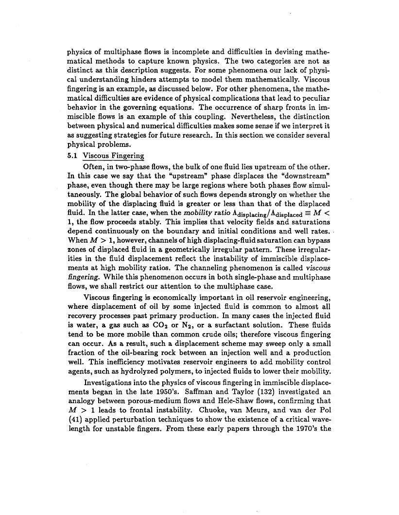
physics of multiphase flows is incomplete and difficulties in devising mathe- matical methods to capture known physics. The two categories are not as distinct as this description suggests. For some phenomena our lack of physi- cal understanding hinders attempts to model them mathematically. Viscous fingering is an example, as discussed below. For other phenomena, the mathe- matical difficulties are evidence of physical complications that lead to peculiar behavior in the governing equations. The occurrence of sharp fronts in im- miscible flows is an example of this coupling. Nevertheless, the distinction between physical and numerical difficulties makes some sense if we interpret it as suggesting strategies for future research. In this section we consider several physical problems . 5.1 Viscous Fingering

Often, in two-phase flows, the bulk of one fluid lies upstream of the other. In this case we say that the “upstream” phase displaces the “downstream” phase, even though there may be large regions where both phases flow simul- taneously. The global behavior of such flows depends strongly on whether the mobility of the displacing fluid is greater or less than that of the displaced fluid. In the latter case, when the mobility ratio Adisplacing/Adisplaced M < 1, the flow proceeds stably. This implies that velocity fields and saturations depend continuously on the boundary and initial conditions and well rates. .

When M > 1, however, channels of high displacing-fluid saturation can bypass zones of displaced fluid in a geometrically irregular pattern. These irregular- ities in the fluid displacement reflect the instability of immiscible displace- ments at high mobility ratios. The channeling phenomenon is called viscous fingering. While this phenomenon occurs in both single-phase and multiphase flows, we shall restrict our attention to the multiphase case.

Viscous fingering is economically important in oil reservoir engineering, where displacement of oil by some injected fluid is common to almost all recovery processes past primary production. In many cases the injected fluid is water, a gas such as COa or Na, or a surfactant solution. These fluids tend to be more mobile than common crude oils; therefore viscous fingering can occur. As a result, such a displacement scheme may sweep only a small fraction of the oil-bearing rock between an injection well and a production well. This inefficiency motivates reservoir engineers to add mobility control agents, such as hydrolyzed polymers, to injected fluids to lower their mobility.

Investigations into the physics of viscous fingering in immiscible displace- ments began in the late 1950’s. Saffman and Taylor (132) investigated an analogy between porous-medium flows and Hele-Shaw flows, confirming that Ad > 1 leads to frontal instability. Chuoke, van Meurs, and van der Pol (41) applied perturbation techniques to show the existence of a critical wave- length for unstable fingers. From these early papers through the 1970’s the

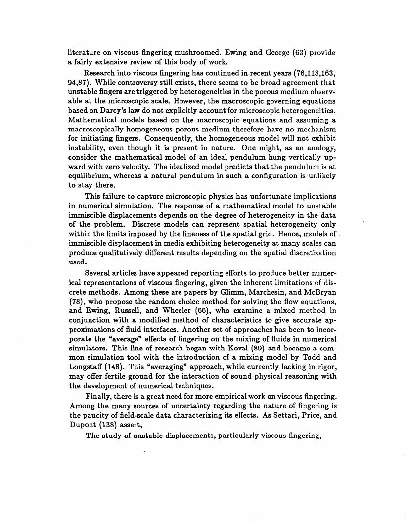
literature on viscous fingering mushroomed. Ewing and George (63) provide a fairly extensive review of this body of work.

Research into viscous fingering has continued in recent years (76,118,163, 94,87). While controversy still exists, there seems to be broad agreement that unstable fingers are triggered by heterogeneities in the porous medium observ- able at the microscopic scale. However, the macroscopic governing equations based on Darcy’s law do not explicitly account for microscopic heterogeneities. Mathematical models based on the macroscopic equations and assuming a macroscopically homogeneous porous medium therefore have no mechanism for initiating fingers. Consequently, the homogeneous model will not exhibit instability, even though it is present in nature. One might, as an analogy, consider the mathematical model of an ideal pendulum hung vertically up- ward with zero velocity. The idealized model predicts that the pendulum is at equilibrium, whereas a natural pendulum in such a configuration is unlikely to stay there.

This failure to capture microscopic physics has unfortunate implications in numerical simulation. The response of a mathematical model to unstable immiscible displacements depends on the degree of heterogeneity in the data of the problem. Discrete models can represent spatial heterogeneity only within the limits imposed by the fineness of the spatial grid. Hence, models o f . immiscible displacement in media exhibiting heterogeneity at many scales can produce qualitatively different results depending on the spatial discretization used.

Several articles have appeared reporting efforts to produce better numer- ical representations of viscous fingering, given the inherent limitations of dis- crete methods. Among these are papers by Glimm, Marchesin, and McBryan (78), who propose the random choice method for solving the flow equations, and Ewing, Russell, and Wheeler (66), who examine a mixed method in conjunction with a modified method of characteristics to give accurate ap- proximations of fluid interfaces. Another set of approaches has been to incor- porate the “average” effects of fingering on the mixing of fluids in numerical simulators. This line of resemch began with Koval (89) and became a com- mon simulation tool with the introduction of a mixing model by Todd and Longstaff (148). This “averaging” approach, while currently lacking in rigor, may offer fertile ground for the interaction of sound physical reasoning with the development of numerical techniques.

Finally, there is a great need for more empirical work on viscous fingering. Among the many sources of uncertainty regarding the nature of fingering is the paucity of field-scale data characterizing its effects. As Settari, Price, and Dupont (138) assert,

The study of unstable displacements, particularly viscous fingering,

\

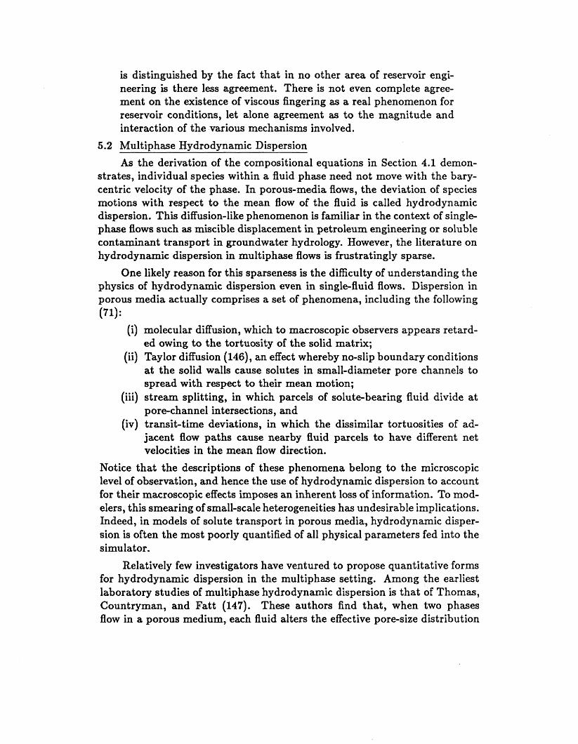
is distinguished by the fact that in no other area of reservoir engi- neering is there less agreement. There is not even complete agree- ment on the existence of viscous fingering as a real phenomenon for reservoir conditions, let alone agreement as to the magnitude and interaction of the various mechanisms involved.

5.2 Multiphase Hydrodynamic Dispersion As the derivation of the compositional equations in Section 4.1 demon-

strates, individual species within a fluid phase need not move with the bary- centric velocity of the phase. In porous-media flows, the deviation of species motions with respect to the mean flow of the fluid is called hydrodynamic dispersion. This diffusion-like phenomenon is familiar in the context of single- phase flows such as miscible displacement in petroleum engineering or soluble contaminant transport in groundwater hydrology. However, the literature on hydrodynamic dispersion in multiphase flows is frustratingly sparse.

One likely reason for this sparseness is the difficulty of understanding the physics of hydrodynamic dispersion even in single-fluid flows. Dispersion in porous media actually comprises a set of phenomena, including the following (71):

(i) molecular diffusion, which to macroscopic observers appears retard- ed owing to the tortuosity of the solid matrix;

(ii) Taylor diffusion (146), an effect whereby no-slip boundary conditions at the solid walls cause solutes in small-diameter pore channels to spread with respect to their mean motion;

(iii) stream splitting, in which parcels of solute-bearing fluid divide at pore-channel intersections, and

(iv) transit-time deviations, in which the dissimilar tortuosities of ad- jacent flow paths cause nearby fiuid parcels to have different net velocities in the mean flow direction.

Notice that the descriptions of these phenomena belong to the microscopic level of observation, and hence the use of hydrodynamic dispersion to account for their macroscopic effects imposes an inherent loss of information. To mod- elers, this smearing of small-scale heterogeneities has undesirable implications. Indeed, in models of solute transport in porous media, hydrodynamic disper- sion is often the most poorly quantified of all physical parameters fed into the simulator.

Relatively few investigators have ventured to propose quantitative forms for hydrodynamic dispersion in the multiphase setting. Among the earliest laboratory studies of multiphase hydrodynamic dispersion is that of Thomas, Countryman, and Fatt (147). These authors find that, when two phases flow in a porous medium, each fluid alters the effective pore-size distribution

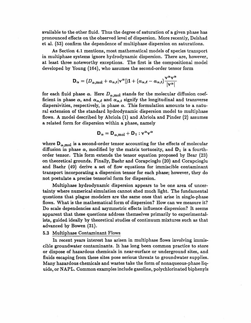
available to the other fluid. Thus the degree of saturation of a given phase has pronounced effects on the observed level of dispersion. More recently, Delshad et al. (53) confirm the dependence of multiphase dispersion on saturations.

As Section 4.1 mentions, most mathematical models of species transport in multiphase systems ignore hydrodynamic dispersion. There are, however, at least three noteworthy exceptions. The first is the compositional model developed by Young (164), who assumes the second-order tensor form

for each fluid phase a. Here Da,mol stands for the molecular diffusion coef- ficient in phase a, and a, ,~ and aa,t signify the longitudinal and transverse dispersivities, respectively, in phase a. This formulation amounts to a natu- ral extension of the standard hydrodynamic dispersion model to multiphase flows. A model described by Abriola (1) and Abriola and Pinder (2) assumes a related form for dispersion within a phase, namely

where Da,mol is a second-order tensor accounting for the effects of molecular diffusion in phase a, modified by the matrix tortuosity, and D1 is a fourth- order tensor. This form extends the tensor equation proposed by Bear (23) on theoretical grounds. Finally, Baehr and Corapcioglu (20) and Corapcioglu and Baehr (49) derive a set of flow equations for immiscible contaminant transport incorporating a dispersion tensor for each phase; however, they do not postulate a precise tensorial form for dispersion.

Multiphase hydrodynamic dispersion appears to be one area of uncer- tainty where numerical simulation cannot shed much light. The fundamental questions that plague modelers are the same ones that arise in single-phase flows. What is the mathematical form of dispersion? How can we measure it? Do scale dependencies and asymmetric effects influence dispersion? It seems apparent that these questions address themselves primarily to experimental- ists, guided ideally by theoretical studies of continuum mixtures such as that advanced by Bowen (31). 5.3 Multiphase Contaminant Flows

In recent years interest has arisen in multiphase flows involving immis- cible groundwater contaminants. It has long been common practice to store or dispose of hazardous chemicals in near-surface or underground sites, and fluids escaping from these sites pose serious threats to groundwater supplies. Many hazardous chemicals and wastes take the form of nonaqueous-phase liq- uids, or NAPL. Common examples include gasoline, polychlorinated biphenyls

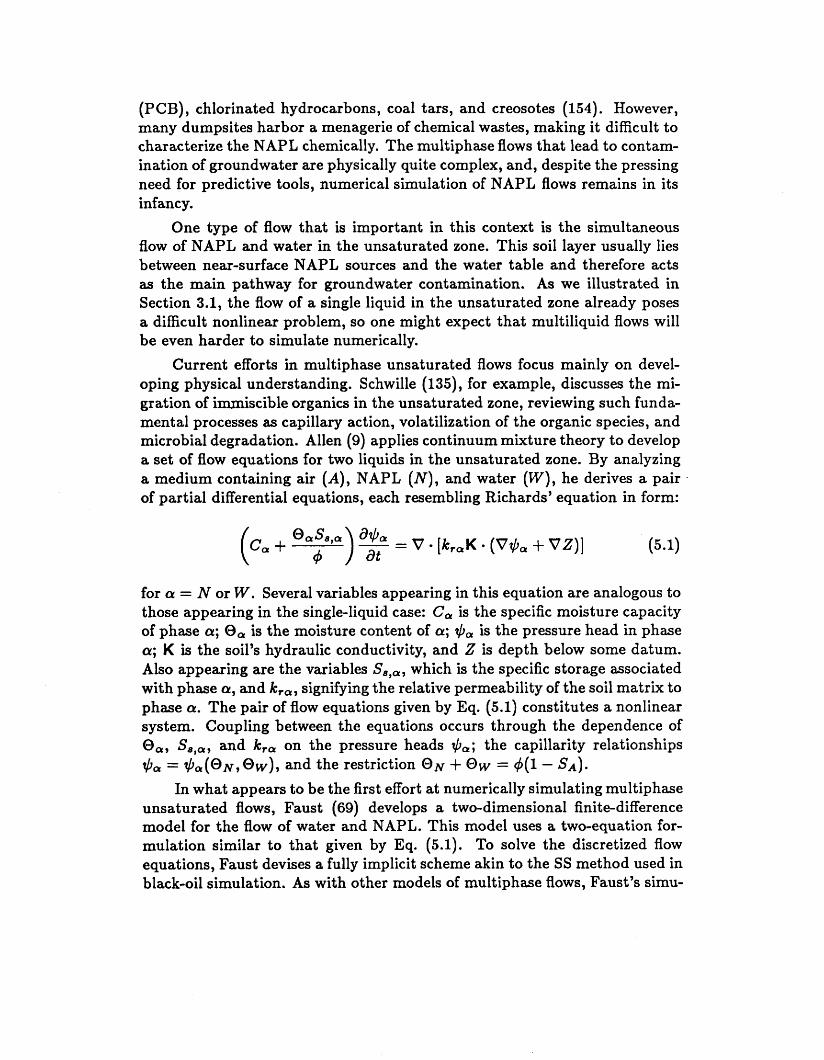
(PCB), chlorinated hydrocarbons, coal tars, and creosotes (154). However, many dumpsites harbor a menagerie of chemical wastes, making it difficult to characterize the NAPL chemically. The multiphase flows that lead to contam- ination of groundwater are physically quite complex, and, despite the pressing need for predictive tools, numerical simulation of NAPL flows remains in its infancy.

One type of flow that is important in this context is the simultaneous flow of NAPL and water in the unsaturated zone. This soil layer usually lies between near-surface NAPL sources and the water table and therefore acts as the main pathway for groundwater contamination. As we illustrated in Section 3.1, the flow of a single liquid in the unsaturated zone already poses a difficult nonlinear problem, so one might expect that multiliquid flows will be even harder to simulate numerically.

Current efforts in multiphase unsaturated flows focus mainly on devel- oping physical understanding. Schwille (135), for example, discusses the mi- gration of immiscible organics in the unsaturated zone, reviewing such funda- mental processes as capillary action, volatilization of the organic species, and microbial degradation. Allen (9) applies continuum mixture theory to develop a set of flow equations for two liquids in the unsaturated zone. By analyzing a medium containing air (A), NAPL (N), and water (W), he derives a pair of partial differential equations, each resembling Richards’ equation in form:

C, + % = V [k,,K (V& + VZ)] 4 for a = N or W. Several variables appearing in this equation are analogous to those appearing in the single-liquid case: C, is the specific moisture capacity of phase a; 0, is the moisture content of a; $, is the pressure head in phase a; K is the soil’s hydraulic conductivity, and 2 is depth below some datum. Also appearing are the variables which is the specific storage associated with phase a, and k,,, signifying the relative permeability of the soil matrix to phase a. The pair of flow equations given by Eq. (5.1) constitutes a nonlinear system. Coupling between the equations occurs through the dependence of O,, and k,, on the pressure heads $,; the capillarity relationships $, = $ , ( O N , @ W ) , and the restriction ON + OW = +(l - SA).

In what appears to be the first effort at numerically simulating multiphase unsaturated flows, Faust (69) develops a two-dimensional finite-difference model for the flow of water and NAPL. This model uses a two-equation for- mulation similar to that given by Eq. (5.1). To solve the discretized flow equations, Faust devises a fully implicit scheme akin to the SS method used in black-oil simulation. As with other models of multiphase flows, Faust’s simu-

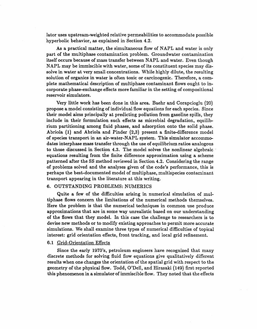
lator uses ups t r eam-weighted relative p ermeab ili t ies to accommodate possible hyperbolic behavior, as explained in Section 4.2.

As a practical matter, the simultaneous flow of NAPL and water is only part of the multiphase contamination problem. Groundwater contamination itself occurs because of mass transfer between NAPL and water. Even though NAPL may be immiscible with water, some of its constituent species may dis- solve in water at very small concentrations. While highly dilute, the resulting solution of organics in water is often toxic or carcinogenic. Therefore, a com- plete mathematical description of multiphase contaminant flows ought to in- corporate phase-exchange effects more familiar in the setting of compositional reservoir simulators.

Very little work has been done in this area. Baehr and Corapcioglu (20) propose a model consisting of individual flow equations for each species. Since their model aims principally at predicting pollution from gasoline spills, they include in their formulation such effects as microbial degradation, equilib- rium partitioning among fluid phases, and adsorption onto the solid phase. Abriola (1) and Abriola and Pinder (2,3) present a finite-difference model of species transport in an air-water-NAPL system. This simulator accommo- dates interphase mass transfer through the use of equilibrium ratios analogous to those discussed in Section 4.3. The model solves the nonlinear algebraic equations resulting from the finite difference approximation using a scheme patterned after the SS method reviewed in Section 4.2. Considering the range of problems solved and the analyses given of the code’s performance, this is perhaps the best-documented model of multiphase, multispecies contaminant transport appearing in the literature at this writing. 6. OUTSTANDING PROBLEMS: NUMERICS

Quite a few of the difficulties arising in numerical simulation of mul- tiphase flows concern the limitations of the numerical methods themselves. Here the problem is that the numerical techniques in common use produce approximations that are in some way unrealistic based on our understanding of the flows that they model. In this case the challenge to researchers is to devise new methods or to modify existing approaches to permit more accurate simulations. We shall examine three types of numerical difficulties of topical interest: grid orientation effects, front tracking, and local grid refinement.

6.1 Grid-Orientation Effects Since the early 1970’s, petroleum engineers have recognized that many

discrete methods for solving fluid flow equations give qualitatively different results when one changes the orientation of the spatial grid with respect to the geometry of the physical flow. Todd, O’Dell, and Hirasaki (149) first reported this phenomenon in a simulator of immiscible flow. They noted that the effects

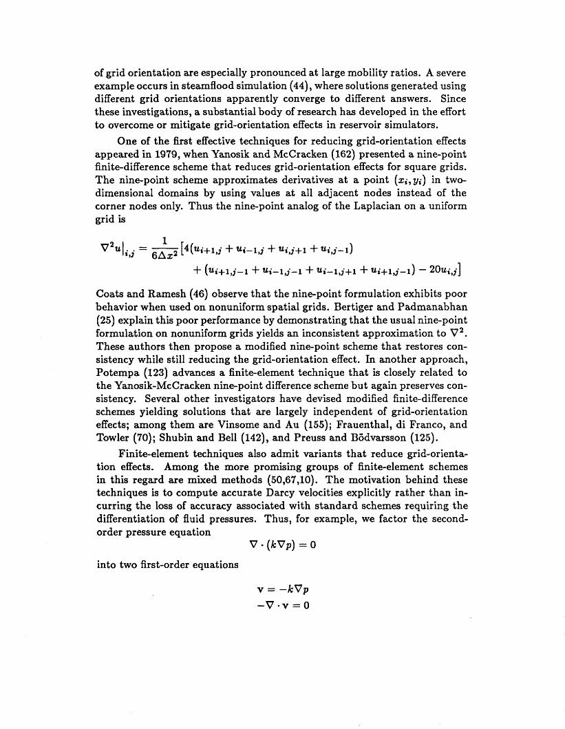
of grid orientation are especially pronounced at large mobility ratios. A severe example occurs in steamflood simulation (44), where solutions generated using different grid orientations apparently converge to different answers. Since these investigations, a substantial body of research has developed in the effort to overcome or mitigate grid-orientation effects in reservoir simulators.

One of the first effective techniques for reducing grid-orientation effects appeared in 1979, when Yanosik and McCracken (162) presented a nine-point finite-difference scheme that reduces grid-orientation effects for square grids. The nine-point scheme approximates derivatives at a point (z;, y;) in two- dimensional domains by using values at all adjacent nodes instead of the corner nodes only. Thus the nine-point analog of the Laplacian on a uniform grid is

Coats and Ramesh (46) observe that the nine-point formulation exhibits poor behavior when used on nonuniform spatial grids. Bertiger and Padmanabhan (25) explain this poor performance by demonstrating that the usual nine-point formulation on nonuniform grids yields an inconsistent approximation to V2. These authors then propose a modified nine-point scheme that restores con- sistency while still reducing the grid-orientation effect. In another approach, Potempa (123) advances a finite-element technique that is closely related to the Yanosik-McCracken nine-point difference scheme but again preserves con- sistency. Several other investigators have devised modified finite-difference schemes yielding solutions that are largely independent of grid-orient ation effects; among them are Vinsome and Au (155); Frauenthal, di Franco, and Towler (70); Shubin and Bell (142), and Preuss and Btidvarsson (125).

Finite-element techniques also admit variants that reduce grid-orienta- tion effects. Among the more promising groups of finite-element schemes in this regard are mixed methods (50,67,10). The motivation behind these techniques is to compute accurate Darcy velocities explicitly rather than in- curring the loss of accuracy associated with standard schemes requiring the differentiation of fluid pressures. Thus, for example, we factor the second- order pressure equation

V (kVp) = O

into two first-order equations

v = - k V p - v * v = 0

By properly choosing the trial functions for v and p, we can compute pressures and velocities having the same order of accuracy. In problems involving the effects of species transport the mixed method is especially effective when used in conjunction with time-stepping procedures based on modified methods of characteristics (67). A variety of numerical experiments reported in the ref- erences cited above demonstrate the method’s ability to give good numerical results even in problems with highly variable material properties. 6.2 Front-Tracking Methods

As we have seen in previous sections, several multiphase flows in porous media exhibit sharp fronts that can be modeled as discontinuous fluid in- terfaces. The saltwater toe and the Buckley-Leverett saturation shock are two examples of such discontinuities. Discrete approximations using fixed finite elements or finite-difference cells have difficulty in capturing the behav- ior of these sharp fronts, since the computational procedures tend to smear information over the spatial subregions of the discretizations. Front-tracking methods aim at circumventing this difficulty by assigning computational de- grees of freedom to the unknown location of the front. Solving for the frontal locations along with the variables characterizing the smooth parts of the flow allows the modeler to track the front explicitly without introducing numerical diffusion. Since one can concentrate many degrees of freedom at the interface, front tracking methods also hold great promise in the simulation of viscous fingering.

Front-tracking methods have their roots in numerical applications of the method of characteristics in convection-dominated flows. The first appli- cations of this approach in porous-media simulation addressed the miscible transport of solutes in single-phase flows (73,120). In the method of charac- teristics, one replaces a partial differential equation by a system of ordinary differential equations valid along curves where the original equation agrees with the chain rule. For example, by comparing the Buckley-Leverett satu- ration equation

with the chain rule dtdSw dxdSw dSw -- +---- -

one can see that dSw/d[ = 0 along curves E(x,t) in the (x,t)-plane where dz/dt = qfb(Sw)/4. Loci of constant SW therefore travel with speed qf&(Sw)/b. This fact allows us to compute the position of the constant= saturation shock as it moves across a one-dimensional domain.

Perhaps the most extensively applied front-tracking scheme in the current literature is that of Glimm and his coworkers (77,79,93). This approach uses

d [ dt d c a x dE

an IMPES formulation for two-dimensional immiscible displacements in the absence of capillarity. The scheme solves the pressure equation on a finite- element grid whose element boundaries move to align themselves with the saturation shock. To update saturations, the scheme uses standard interior methods in regions where the saturation is smooth and couples to the smooth solution a Riemann problem propagating the interface. This frontal propaga- tion relies on a method of characteristics akin to the one-dimensional version outlined above, taking advantage of a local coordinate system aligned with the shock to advance the discontinuity in its normal direction. Thus the actual computations required to track the front reduce to locally one-dimensional ordinary differential equations.

Jensen and Finlayson (85,86) introduce an alternative scheme for front- tracking that gives good results in convection-dominated species-transport problems. This method defines a set of moving coordinates based on the method of characteristics €or the hyperbolic, or purely convective, part of the partial differential equations. Within this moving coordinate system, the convection-dominated transport problem reduces to a problem of the diffusion type. Jensen and Finlayson construct a finite-element grid attached to the moving coordinates, ensuring that the grid in the vicinity of the sharp front is sufficiently fine to avoid the occurrence of nonphysical oscillations in the numerical solution.

In a third approach to front tracking, the Mathematics Group at the Lawrence Berkeley Laboratory applies the theory of Riemann problems for first-order hyperbolic systems to solve the immiscible flow equations using the random choice method (47,48,4). The random choice method, developed as a numerical technique by Chorin (40), is an effective procedure for ap- proximating nonlinear hyperbolic conservation laws such as Eq. (6.1). The method replaces the unknown function Sw (5, t ) by a piecewise constant ap- proximation & ~ ( z , t ) and then solves a sequence of Riemann problems, each advancing the numerical solution by sampling the piecewise constant function

to determine initial data. When the solution possesses shocks, the random choice method preserves their sharp fronts, since the sampling at each time step avoids the introduction of spurious intermediate values in the numeri- cal solution. However, the method allows small errors in the shock location since the sampling identifies the frontal position only to within the resolution limits imposed by the spatial grid. Although developed for one-dimensional flows, the random choice method admits extensions to two-dimensional prob- lems. Colella, Concus, and Sethian (47) describe the use of operator splitting techniques to decompose a two-dimensional equation into a sequence of one- dimensional equations.

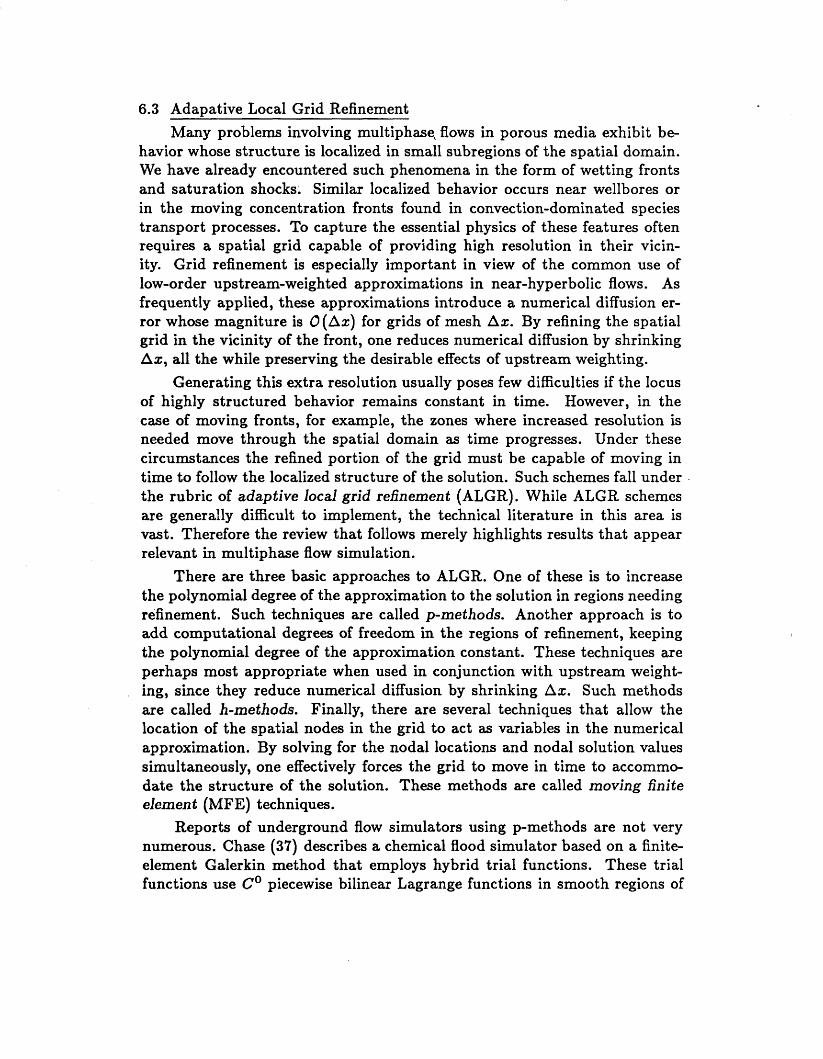
6.3 Adapative Local Grid Refinement Many problems involving multiphase, flows in porous media exhibit be-

havior whose structure is localized in small subregions of the spatial domain. We have already encountered such phenomena in the form of wetting fronts and saturation shocks. Similar localized behavior occurs near wellbores or in the moving concentration fronts found in convection-dominated species transport processes. To capture the essential physics of these features often requires a spatial grid capable of providing high resolution in their vicin- ity. Grid refinement is especially important in view of the common use of low-order upstream-weighted approximations in near-hyperbolic flows. As frequently applied, these approximations introduce a numerical diffusion er- ror whose magniture is O(Az) for grids of mesh Az. By refining the spatial grid in the vicinity of the front, one reduces numerical diffusion by shrinking Az, all the while preserving the desirable effects of upstream weighting.

Generating this extra resolution usually poses few difficulties if the locus of highly structured behavior remains constant in time. However, in the case of moving fronts, for example, the zones where increased resolution is needed move through the spatial domain as time progresses. Under these circumstances the refined portion of the grid must be capable of moving in time to follow the localized structure of the solution. Such schemes fall under the rubric of adaptive local grid refinement (ALGR). While ALGR schemes are generally difficult to implement, the technical literature in this area is vast. Therefore the review that follows merely highlights results that appear relevant in multiphase flow simulation.

There are three basic approaches to ALGR. One of these is to increase the polynomial degree of the approximation to the solution in regions needing refinement. Such techniques are called p-methods. Another approach is to add computational degrees of freedom in the regions of refinement, keeping the polynomial degree of the approximation constant. These techniques are perhaps most appropriate when used in conjunction with upstream weight- ing, since they reduce numerical diffusion by shrinking As. Such methods are called h-methods. Finally, there are several techniques that allow the location of the spatial nodes in the grid to act as variables in the numerical approximation. By solving for the nodal locations and nodal solution values simultaneously, one effectively forces the grid to move in time to accommo- date the structure of the solution. These methods are called moving finite element (MF E) techniques.

Reports of underground flow simulators using p-methods are not very numerous. Chase (37) describes a chemical flood simulator based on a finite- element Galerkin method that employs hybrid trial functions. These trial functions use Co piecewise bilinear Lagrange functions in smooth regions of

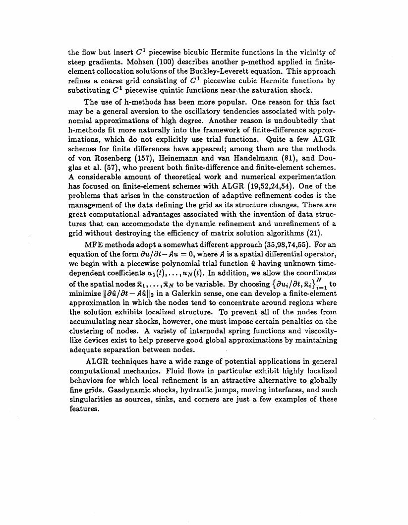
the flow but insert C' piecewise bicubic Hermite functions in the vicinity of steep gradients. Mohsen (100) describes another p-method applied in finite- element collocation solutions of the Buckley-Leverett equation. This approach refines a coarse grid consisting of C1 piecewise cubic Hermite functions by substituting C1 piecewise quintic functions near, the saturation shock.

The use of h-methods has been more popular. One reason for this fact may be a general aversion to the oscillatory tendencies associated with poly- nomial approximations of high degree. Another reason is undoubtedly that h-methods fit more naturally into the framework of finite-difference approx- imations, which do not explicitly use trial functions. Quite a few ALGR schemes for finite differences have appeared; among them are the methods of von Rosenberg (157), Heinemann and van Handelmann (81), and Dou- glas et al. (57), who present both finite-difference and finite-element schemes. A considerable amount of theoretical work and numerical experimentation has focused on finite-element schemes with ALGR (19,52,24,54). One of the problems that arises in the construction of adaptive refinement codes is the management of the data defining the grid as its structure changes. There are great computational advantages associated with the invention of data struc- tures that can accommodate the dynamic refinement and unrefinement of a grid without destroying the efficiency of matrix solution algorithms (21).

MFE methods adopt a somewhat different approach (35,98,74,55). For an equation of the form au/at- A u = 0, where A is a spatial differential operator, we begin with a piecewise polynomial trial function .ii having unknown time- dependent coefficients u1(t), . . . , u ~ ( t ) . In addition, we allow the coordinates of the spatial nodes % I , . . ,%N to be variable. By choosing { a ~ i / d t , R ; ) ~ = ~ to minimize Ila.ii/& - A in a Galerkin sense, one can develop a finite-element approximation in which the nodes tend to concentrate around regions where the solution exhibits localized structure. To prevent all of the nodes from accumulating near shocks, however, one must impose certain penalties on the clustering of nodes. A variety of internodal spring functions and viscosity- like devices exist to help preserve good global approximations by maintaining adequate separation between nodes.

ALGR techniques have a wide range of potential applications in general computational mechanics. Fluid flows in particular exhibit highly localized behaviors for which local refinement is an attractive alternative to globally fine grids. Gasdynamic shocks, hydraulic jumps, moving interfaces, and such singularities as sources, sinks, and corners are just a few examples of these features.

N

7. CONCLUSIONS Throughout this review we have seen several facets of multiphase flows

in porous media reappear in various applications. These physical and com- putational peculiarities emerge as major themes in the numerical simulation of flows. Let us close by recapitulating these themes.

Every flow we have examined obeys a nonlinear, time-dependent partial differential equation. Nonlinearity is a characteristic feature of multiphase porous-media flows, owing to the fact that the permeability of the rock ma- trix to one fluid varies with the saturation of any other fluid. Further non- linearities can arise when storage or compressibility effects imply pronounced dependence on pressure in the accumulation terms or when there is strong coupling within a system of flow equations. The nonlinear governing differ- ential equations generally give rise to nonlinear algebraic equations in the approximating discretizations. These algebraic systems, in turn, demand it- erative solution, and therefore one commonly finds Newton-Raphson schemes or related procedures imbedded in implicit time-stepping methods for these problems.

Another common feature in multiphase porous-media flows is the occur- rence of sharp fronts or moving boundaries in the fluid system. The Buckley- Leverett saturation shock stands as a classic example. Similar interfaces arise in other contexts: unsaturated flows can give rise to wetting fronts, and the saltwater intrusion problem exhibits a moving boundary in the toe of the salt- water wedge. Sharp fronts pose difficulties to the numerical analyst, since they require high spatial resolution to model and are sometimes associated with uniqueness issues. In certain classes of flows they can also exhibit instability, as when viscous fingering occurs in displacements at adverse mobility ratios. The most natural solutions to these sharp-front difficulties are front-tracking methods and adaptive local grid refinement.

Finally, various numerical aspects of modeling multiphase flows combine to require truly large-scale computations. A typical simulator solves large, sparse matrix equations at every iteration of every time step. When com- positional effects are present, the code must solve nonlinear thermodynamic constraints as well. The desirability of local grid enrichment, front-tracking algorithms, or moving grid schemes adds to this scale of calculation both in complexity and in computational effort. Scientists who model multiphase underground flows have every reason to applaud the emerging generation of supercomputers and parallel architectures, since these machines may spell the difference between compromise in the approximation of complex flows and the practical achievement of realis tic simulations.

ACKNOWLEDGMENTS

The Wyoming Water Research Center supported much of this work through a grant to study multiphase contaminant flows. The National Science Foundation provided support through grant number CEE-8404266.

REFERENCES 1

2

3

4

5

6

7

8

9

10

11

12

Abriola, L. M., Multiphase Migration of Organic Compounds in a Porous Medium, Springer-Verlag, Berlin, 1984. Abriola, L. M., and Pinder, G. F., “A Multiphase Approach to the Model- ing of Porous Media Contamination by Organic Compounds 1. Equation Development,” Water Resources Research, Vol. 21, 1985, pp. 11-18. Abriola, L. M., and Pinder, G. F., “A Multiphase Approach to the Model- ing of Porous Media Contamination by Organic Compounds 2. Numerical Simulation,” Water Resources Research, Vol. 21, 1985, pp. 19-26. Albright, N., and Concus, P., “On Calculating Flows with Sharp Fronts in a Porous Medium,” Fluid Mechanics in Energy Conservation, J. D. Buck- master, ed., Society for Industrial and Applied Mathematics, Philadel- phia, Pa., 1980, pp. 172-184. Allen, M. B., “How Upstream Collocation Works,” International Journal for Numerical Methods in Engineering, Vol. 19, 1983, pp. 1753-1763. Allen, M. B., “A Collocation Model of Compositional Oil Reservoir Flows,” Mathematical Methods in Energy Research, K. I. Gross, ed., Society for Industrial and Applied Mathematics, Philadelphia, Pa., 1984,

Allen, M. B., Collocation Techniques for Compositional Flows in Oil Reservoirs, Springer-Verlag, Berlin, 1984. Allen, M. B., “Why Upwinding is Reasonable,” Finite Elements in Water Resources, J. P. Laible et al., eds., Springer-Verlag, Berlin, 1984, pp. 13- 23. Allen, M. B., “Mechanics of Multiphase Fluid Flows in Variably Sat- urated Porous Media,” hternational Journal for Engineering Science, 1985, to appear. Allen, M. B., Ewing, R. E., and Koebbe, J. V., “Mixed Finite-Element Methods for Computing Groundwater Velocities,” Numerical Methods for Partial Differential Equations, 1985, to appear. Allen, M. B., and Murphy, C., “A Finite-Element Collocation Method for Variably Saturated Flows in Porous Media,” Numerical Methods for Partial Differential Equations, to appear. Allen, M. B., and Pinder, G. F., ”Collocation Simulation of Multiphase Porous-Medium Flow,” Society of Petroleum Engineers Journal, 1983,

.

pp. 157-180.

pp. 135-142.

13

14

15

16

17

18

19

20

21

22

23

24

25

Allen, M. B., and Pinder, G. F., “The Convergence of Upstream Colloca- tion in the Buckley-Leverett Problem,” Society of Petroleum Engineers Journal, 1985, to appear. Amaefule, J. O., and Handy, L. L., “The Effect of Interfacial Tensions on Relative Oil/ Water Permeabilities of Consolidated Porous Media,” Society of Petroleum Engineers Journal, 1982, pp. 371-381. Appleyard, J. R., Cheshire, I. M., and Pollard, R. K., “Special Tech- niques for Fully-Implicit Simulators,” Third European Symposium on Enhanced Oil Recovery, F. J. Fayers, ed., Elsevier Scientific Publishing Co., Amsterdam, 1981, pp. 395-408. Aronson, D. G., “Nonlinear Diffusion Problems,” Free Boundary Prob- lems: Theory and Applications, A. Fasano and M. Primicerio, eds., Vol. 1, Pitman Advanced Publishing Program, Boston, Mass., 1983, pp. 135- 149. Atkin, R. J., and Craine, R. E., “Continuum Theories of Mixtures: Ba- sic Theory and Historical Development,” Quarterly Journal of Applied Mathematics, Vol. 29, No. 2, 1976, pp. 209-244. Aziz, K., and Settari, A., Petroleum Reservoir Simulation, Applied Sci- ence Publishers, London, 1979. Babuska, I., and Rheinboldt, W. C., “Error Estimates for Adaptive Finite Element Computations,” Society for Industrial and Applied Mathematics Journal of Numerical Analysis, Vol. 15, 1978, pp. 736-754. Baehr, A., and Corapcioglu, M. Y., “A Predictive Model for Pollution from Gasoline in Soils and Groundwater,” Proceedings, Petroleum Hy- drocarbons and Organic Chemicals in Groundwater: Prevention, Detec- tion, and Restoration, Houston, Tex., 1984. Bank, R. E., and Sherman, A. H., “A Refinement Algorithm and Dy- namic Data Structure for Finite Element Meshes,” Center for Numerical Analysis Technical Report 166, University of Texas, Austin, Tex., 1980. Bardon, C., and Longeron, D. G., “Influence of Interfacial Tensions on Relative Permeability,” Society of Petroleum Engineers Journal, 1980, pp. 391-401. Bear, J., “On the Tensor Form of Dispersion in Porous Media,” Journal of Geophysical Research, Vol. 66, 1961, pp. 1185-1197. Beiterman, M., “A Posteriori Error Estimation and Adaptive Finite Ele- ment Grids for Parabolic Equations,” Adaptive Computational Methods for Partial Differential Equations, I. Babuska et al., eds., Society for In- dustrial and Applied Mathematics, Philadelphia, Pa., 1983, pp. 123-141. Bertiger, W. I., and Padmanabhan, L., “Finite Difference Solutions to Grid Orientation Problems Using IMPES,” Proceedings, Seventh Sym- posium on Reservoir Simulation, Society of Petroleum Engineers, 1983,

pp. 163-172. 26 Birkhoff, G., “Numerical Fluid Dynamics,” Society for Industrial and

Applied Mathematics Review, Vol. 25, 1983, pp. 1-34. 27 BjGrdammen, J. B., and Coats, K. H., “Comparison of Alternating Direc-

tion and Successive Overrelaxation Techniques in Simulation of Reservoir Fluid Flow,” Society of Petroleum Engineers Journal, 1969, pp. 47-58.

28 Blair, P. M., and Weinaug, C. F., “Solution of Two-Phase Flow Prob- lems Using Implicit Finite Differences,” Society of Petroleum Engineers Journal, 1969, pp. 417-424.

29 Bowen, R. M., “Incompressible Porous Media Models by the Use of the Theory of Mixtures,” International Journal of Engineering Science, Vol. 18, 1980, pp. 1129-1148.

30 Bowen, R. M., “Compressible Porous Media Models by the Use of the Theory of Mixtures,” International Journal of Engineering Science,

31 Bowen, R. M., “Diffusion Models Implied by the Theory of Mixtures,” Appendix 5A to Rational Thermodynamics, 2nd ed., by C. A. Truesdell, Springer-Verlag, New York, N.Y., 1984, pp. 237-263.

32 Breitenbach, E. A., Thurnau, D. H., and van Poolen, H. K., “Solution of the Immiscible Fluid Flow Simulation Equation,” Society of Petroleum Engineers JournaI, 1969, pp. 155-169.

33 Bresler, E., “Simultaneous Transport of Solutes and Water Under Tran- sient Unsaturated Flow Conditions,” Water Resources Research, Vol. 9,

34 Buckley, S. E., and Leverett, M. C., “Mechanism of Fluid Displacement in Sands,” Transactions, American Institute of Mining, Metallurgical, and Petroleum Engineers, Vol. 146, 1942, pp. 107-116.

35 Carey, G. F., Mueller, A., Sephehrnoori, K., and Thrasher, R. L., “Mov- ing Elements for Reservoir Transport Processes,” Proceedings, Fifth Sym- posium on Reservoir Simulation, Society of Petroleum Engineers, 1979,

36 Celia, M. A., and Pinder, G. F., “An Analysis of Alternating-Direction Methods for Parabolic Equations,” Numerical Methods for Partial Dif- ferential Equations, Vol. 1, 1985, pp. 57-70.

37 Chase, C. A., “Variational Simulation with Numerical Decoupling and Local Mesh Refinement ,” Proceedings, Fifth Symposium on Reservoir Simulation, Society of Petroleum Engineers, 1979, pp. 73-94.

38 Chien, M. C. H., Lee, S. T., and Chen, W. H., “A New Fully Implicit Compositional Simulator,” Proceedings, Eighth Symposium on Reservoir Simulation, Society of Petroleum Engineers, Feb., 1985, pp. 7-30.

39 Chorin, A. J., and Marsden, J. E., A Mathematical Introduction to Fluid

VO~. 20, 1982, pp. 697-735.

1973, pp. 975-986.

pp. 135-144.

Mechanics, Springer-Verlag, New York, N.Y., 1979, Chapter 3. 40 Chorin, A. J., “Random Choice Solution of Hyperbolic Systems,” Journal

of Computational Physics, Vol. 22, 1976, pp. 517-533. 41 Chuoke, R. L., van Meurs, P., and van der Poel, C., “The Instability

of Slow, Immiscible, Liquid-Liquid Displacements in Permeable Media,” Society of Petroleum Engineers Journal, 1959, pp. 188-194.

42 Coats, K., “An Equation-of-State Compositional Model,” Society of Pe- troleum Engineers Journal, 1980, pp. 363-376.

43 Coats, K., “Reservoir Simulation: State of the Art,” Journal of Petroleum Technology, 1982, pp. 1633-1642.

44 Coats, K. H., George, W. D., Chu, C., and Marcum, B. E., “Three- Dimensional Simulation of Steamflooding,” presented at the Sept. 30- Oct. 3, 1973, Annual Fall Technical Conference and Exhibition of the Society of Petroleum Engineers.

45 Coats, K. H., Nielsen, R. L., Terhune, M. H., and Weber, A. G., “Simula- tion of Three-Dimensional, Two-Phase Flow in Oil and Gas Reservoirs,” Society of Petroleum Engineers Journal, 1967, pp. 377-388.

46 Coats, K. H., and Ramesh, A. B., “Effect of Grid Type and Difference Scheme on Pattern Steamflood Results,” presented at the Sept. 26- 29, 1982, Fall Technical Conference and Exhibition of the Society of Petroleum Engineers.

47 Colella, P., Concus, P., and Sethian, J., “Some Numerical Methods for Discontinuous Flows in Porous Media,” The Mathematics of Reservoir Simulation, R. E. Ewing, ed., Society for Industrial and Applied Mathe- matics, Philadelphia, Pa., 1983, pp. 161-186.

48 Concus, P., “Calculation of Shocks in Oil Reservoir Modeling and Porous Flow,” Numerical Methods for Fluid Dynamics, K. W. Morton and M. J. Baines, eds., Academic Press, New York, N.Y., 1982, pp. 165-178.

49 Corapcioglu, M. Y., and Baehr, A., “Immiscible Contaminant Transport in Soils and Groundwater with an Emphasis on Petroleum Hydrocarbons: System of Differential Equations vs. Single Cell Model,” Water Sciences and Technology, 1985, to appear.

50 Darlow, B. L., Ewing, R. E., and Wheeler, M. F., “Mixed Finite Element Methods for Miscible Displacement Problems in Porous Media,” Proceed- ings, Sixth Symposium on Reservoir Simulation, Society of Petroleum Engineers, 1982, pp. 137-146.

51 Davis, H. T., and Scriven, L. E., “The Origins of Low Interfacial Ten- sions for Enhanced Oil Recovery,” presented at the September 21-24, 1980, Annual Fall Technical Conference and Exhibition of the Society of Petroleum Engineers of AIME.

52 Davis, S., and Flaherty, J., “An Adaptive Finite Element Method for

Initial-Boundary Value Problems for Partial Differential Equations,” So- ciety for Industrial and Applied Mathematics Journal for Scientific and Statistical Computing, Vol. 3, 1983, pp. 6-27.

53 Delshad, M., MacAllister, D. J., Pope, G. A., and Rouse, B. A., “Multi- phase Dispersion and Relative Permeability Experiments,” presented at the Sept., 1982, Society of Petroleum Engineers Annual Fall Technical Conference and Exhibition, held in New Orleans, La.

54 Diaz, J. C., Ewing, R. E., Jones, R. W., McDonald, A. E., Uhler, L. M., and von Rosenberg, D. U., “Self Adaptive Local Grid Refinement in Enhanced Oil Recovery,” Proceedings, Fifth International Symposium on Finite Elements and Flow Problems, Austin, Tex., Jan. 23-26, 1984, pp. 479-484.

55 Djomehri, M. J., and Miller, K., “A Moving Finite Element Code for General Systems of Partial Differential Equations in Two Dimensions,” University of California Center for Pure aad Applied Mathematics Re- port PAM-57, Berkeley, Calif., Oct., 1981.

56 Douglas, J., Jr., “Alternating Direction Methods for Three Space Vari- ables,” Numerische Mathematik, Vol. 2 , 1962, pp. 91-98.

57 Douglas, J., Jr., Darlow, B. L., Wheeler, M. F., and Kendall, R. P., “Self-Adaptive Finite Element and Finite Difference Methods for One- Dimensional Two-Phase Immiscible Flow,” Computer Methods in Ap- plied Mechanics and Engineering, Vol. 47, 1984, pp. 119-130.

58 Douglas, J., Jr., and Dupont, T., “A Finite-Element Collocation Method for Quasilinear Parabolic Equations,” Mathematics of Computation,

59 Douglas, J., Jr., Peaceman, D. W., and Rachford, H. H., Jr., “A Method for Calculating Multidimensional Immiscible Displacement ,” Transac- tions, American Institute of Mining, Metallurgical, and Petroleum Engi- neers, Vol. 216, 1959, pp. 297-306.

60 Douglas, J., Jr., and Rachford, H. H., Jr., “On the Numerical Solution of Heat Conduction Problems in Two and Three Space Variables,” Trans- actions, American Mathematical Society, Vol. 82, 1956, pp. 421-439.

61 Eringen, A. C., and Ingram, J. D., “A Continuum Theory of Chemically Reacting Media-I,” International Journal of Engineering Science, Vol. 3,

62 Ewing, R. E., “Alternating-Direction Galerkin Methods for Parabolic, Hyperbolic, and Sobolev Partial Differential Equations,” Proceedings of the Special Year in Numerical Analysis, University of Maryland, College Park, Md., 1981, pp. 123-150.

63 Ewing, R. E., and George, J. H., “Viscous Fingering in Hydrocarbon Re- covery Processes,” Mathematical Methods in Energy Research,

VO~. 27, pp. 17-28.

1965, pp. 197-212.

K. I. Gross, ed., Society for Industrial and Applied Mathematics, Philadel- phia, Pa., 1984, pp. 194-213.

64 Ewing, R. E., and Heinemann, R. F., “Incorporation of Mixed Finite El- ement Methods in Compositional Simulation for Reduction of Numerical Dispersion,” Proceedings, Seventh Symposium on Reservoir Simulation, Society of Petroleum Engineers, Nov., 1983, pp. 341-347.

65 Ewing, R. E., and Heinemann, R. F., “Mixed Finite Element Approxima- tion of Phase Velocities in Compositional Reservoir Simulation,” Com- puter Methods in Applied Mechanics and Engineering, Vol. 47, 1984,

66 Ewing, R. E., Russell, T. F., and Wheeler, M. F., “Simulation of Miscible Displacement Using Mixed Methods and a Modified Method of Char- acteristics,’’ Proceedings, Seventh Symposium on Reservoir Simulation, Society of Petroleum Engineers, 1983, pp. 71-82.

67 Ewing, R. E., Russell, T. F., and Wheeler, M. F., “Convergence Analysis of an Approximation of Miscible Displacement in Porous Media by Mixed Finite Elements and a Modified Method of Characteristics,” Computer Methods in Applied Mechanics and Engineering, Vol. 47,1984, pp. 73-92.

68 Fatt, I., and Dykstra, H., “Relative Permeability Studies,” Transactions, American Institute of Mining, Metallurgical, and Petroleum Engineers, Vol. 192, 1951, pp. 249-256.

69 Faust, C. R., “Transport of Immiscible Fluids Within and Below the Un- saturated Zone: A Numerical Model,” Water Resources Research, Vol. 21,

70 Frauenthal, J. C., di Franco, R. B., and Towler, B. F., “Reduction of Grid Orientation Effects in Reservoir Simulation Using Generalized Upstream Weighting,” Proceedings, Seventh Symposium on Reservoir Simulation, Society of Petroleum Engineers, 1983, pp. 7-16.

71 Fried, J. J., Groundwater Pollution, Elsevier Scientific Publishing Co., Amsterdam, 1975.

72 Fussell, L. T., and Fussell, D. D., “An Iterative Technique for Composi- tional Reservoir Models,” Society of Petroleum Engineers Journal, 1979, pp. 211-220.

73 Garder, A. O., Peaceman, D. W., and Pozzi, A. L., “Numerical Cal- culation of Multidimensional Miscible Displacement by the Method of Characteristics,” Society of Petroleum Engineers Journal, 1964, pp. 26- 36.

74 Gelinas, R. J., DOSS, S. K., and Miller, K., “The Moving Finite El- ement Method: Applications to General Partial Differential Equations with Large Multiple Gradients,” Journal of Computational Physics,

pp. 161-176.

1985, pp. 587-596.

Vol. 40, 1981, pp. 202-221.

75 Gibbs, J. W., “On the Equilibrium of Heterogeneous Substances,” Trans- actions, Connecticut Academy, Vol. 3, 1876, pp. 108-248, and 1878,

76 Glimm, J., Isaacson, E. L., Lindquist, B., McBryan, O., and Yaniv, S., “Statistical Fluid Dynamics: The Influence of Geometry on Surface In- stabilities,” The Mathematics of Reservoir Simulation, R. E. Ewing, ed., Society for Industrial and Applied Mathematics, Philadelphia, Pa., 1983,

77 Glimm, J., Lindquist, B., McBryan, O., and Padmanabhan, L., “A Front Tracking Reservoir Simulator, Five-Spot Validation Studies, and the Wa- ter Coning Problem,” The Mathematics of Reservoir Simulation, R. E. Ewing, ed., Society for Industrial and Applied Mathematics, Phila- delphia, Pa., 1983, pp. 107-135.

78 Glimm, J., Marchesin, D., and McBryan, O., “A Numerical Method for Two-Phase Flow with an Unstable Interface,” Journal of Computational Physics, Vol. 39, 1981, pp. 179-200.

79 Glimm, J., Marchesin, D., and McBryan, O., “A Numerical Method for Two Phase Flows with an Unstable Interface,” Journal of Computational Physics, Vol. 39, 1981, pp. 91-119.

80 Heinemann, R. F., “Simulation of Compositional Oil Recovery Processes,” Mathematical Methods in Energy Research, K. I. Gross, ed., Society for Industrial and Applied Mathematics, Philadelphia, Pa., 1984, pp. 214- 235.

81 Heinemann, 2. E., and von Hantelmann, G., “Using Local Grid Refine- ment in a Multiple Application Reservoir Simulator,” Proceedings, Sev- enth Symposium on Reservoir Simulation, Society of Petroleum Engi- neers, 1983, pp. 205-218.

82 Hoa, N. T., Gaudu, R., and Thirriot, C., “Influence of the Hysteresis Ef- fect on Transient Flows in Saturated-Unsaturated Porous Media,” Water Resources Research, Vol. 13, 1977, pp. 992-996.

83 Huyakorn, P. S., and Pinder, G. F., “A New Finite Element Technique for the Solution of Two-Phase Flow Through Porous Media,” Advances in Water Resources, Vol. 1, 1978, pp. 285-298.

84 Huyakorn, P. S., and Pinder, G. F., Computational Methods in Subsur- face Flow, Academic Press, New York, N.Y., 1983.

85 Jensen, 0. K., and Finlayson, B. A,, “A Solution of the Transport Equa- tion Using a Moving Coordinate System,” Advanced in Water Resources, Vol. 3, 1980, pp. 9-18.

86 Jensen, 0. K., and Finlayson, B. A., “A Numerical Technique for Track- ing Sharp Fronts in Studies of Tertiary Oil Recovery Pilots,” Proceed- ings, Seventh Symposium on Reservoir Simulation, Society of Petroleum

pp. 343-524.

pp. 137-160.

Engineers, 1983, pp. 61-70. 87 Jerrauld, G. R., Davis, H. T., and Scriven, L. E., “Frontal Structure and

Stability in Immiscible Displacement ,” Proceedings, Fourth Symposium on Enhanced Oil Recovery, Society of Petroleum Engineers and U.S. De- partment of Energy, Vol. 2, 1984, pp. 135-144.

88 Kazemi, H., Vestal, C. R., and Shank, G. D., “An Efficient Multicom- ponent Numerical Simulator,” Society of Petroleum Engineers Journal,

89 Koval, E. J., “A Method for Predicting the Performance of Unsteady Miscible Displacement ,” Society of Petroleum Engineers, 1963, pp. 145- 154.

90 Lax, P. D., “Hyperbolic Systems of Conservation Laws 11,” Communica- tions in Pure and Applied Mathematics, Vol. 10, 1957, pp. 537-566.

91 Leverett, M. C., “Capillary Behavior in Porous Solids,” Transactions, American Institute of Mining, Metallurgical, and Petroleum Engineers, Vol. 142, 1941, pp. 159-169.

92 Leverett, M. C., and Lewis, W. B., “Steady Flow of Gas-Oil-Water Mix- tures Through Unconsolidated Sands,” Transactions, American Insti- tute of Mining, Metallurgical, and Petroleum Engineers, Vol. 142, 1941,

93 McBryan, O., “Shock Tracking Methods in 2-D Flows,” Ninth National Applied Mechanics Congress, Cornell University, Ithaca, N.Y., 1982.

94 McLean, J. W., “The Fingering Problem in Flow Through Porous Me- dia,” thesis presented to the California Institute of Technology, at Pasa- dena, Cal., in 1980 in partial fulfillment of the requirements for the degree of Doctor of Philosophy.

95 Meijerink, J. A., and Van der Vorst, H. A., “An Iterative Solution Method for Linear Systems of Which the Coefficient Matrix is a Symmetric M- Matrix,” Mathematics of Computation, Vol. 31, 1977, pp. 148-162.

96 Mercer, J. W., and Faust, C. R., “The Application of Finite Element Techniques to Immiscible Flow in Porous Media,” Finite Elements in Water Resources, W. G . Gray et al., eds., London, Pentech Press, 1977,

97 Mercer, J. W., Larson, S. P., and Faust, C. R., “Simulation of Salt-Water Interface Motion,” Ground Water, Vol. 18, 1980, pp. 374-385.

98 Miller, K., and Miller, R. N., “Continuously Deforming Finite Elements, I,” Society for Industrial and Applied Mathematics Journal of Numerical Analysis, Vol. 18, 1981, pp. 1019-1032.

99 Milly, P. C. D., “A Mass-Conservative Procedure for Time-Stepping in Models of Unsaturated Flow,” Finite Elements in Water Resources, J. P. Laible et al., eds., Springer-Verlag, London, 1984, pp. 103-112.

1978, pp. 355-368.

pp. 107-120.

pp. 21-43.

100 Mohsen, M. F. N., “Numerical Experiments Using ‘Adaptive’ Finite Ele- ments with Collocation,” Finite Elements in Water Resources, J. P. Laible et al., eds., Springer-Verlag, Berlin, 1984, pp. 45-61.

101 Molina, N. M., “A Systematic Approach to the Relative Permeability Problem in Reservoir Simulation,” presented at the September 21-24, 1980, Annual Fall Technical Conference and Exhibition of the Society of Petroleum Engineers of AIME.

102 Morel-Seytoux, H. J., “Introduction to Flow of Immiscible Liquids in Porous Media,” Flow Through Porous Media, R. J. M. De Weist, ed., Academic Press, New York, N.Y., 1969, pp. 456-516.

103 Morrow, N. R., “Physics and Thermodynamics of Capillary Action in Porous Media,” Symposium on Flow Through Porous Media, R. Nunge, ed., American Chemical Society Publications, Washington, D.C., 1969,

104 Muskat, M., Wykoff, R. D., Botset, H. G., and Meres, M. W., “Flow of Gas-Liquid Mixtures Through Sands,” Transactions, American Insti- tute of Mining, Metallurgical, and Petroleum Engineers, Vol. 123, 1937, pp. 69-96.

105 Nakano, Y., “Application of Recent Results in Functional Analysis to the Problem of Wetting Fronts,” Water Resources Research, Vol. 16, 1980,

106 Narasimhan, T. N., and Witherspoon, P. A., “Numerical Model for Satu- rated-Unsaturated Flow in Deformable Porous Media 3. Applications,” Water Resources Research, Vol. 14, 1978, pp. 1017-1033.

107 Neumann, S. P., “Saturated-Unsaturated Seepage by Finite Elements,” Journal of the Hydraulics Division of ASCE, Vol. 99,1973, pp. 2233-2251.

108 Nghiem, L. X., Fong, D. K., and Aziz, K., “Compositional Modeling with an Equation of State,” Society of Petroleum Engineers Journal, 1981,

109 Nolen, J. S., “Numerical Simulation of Compositional Phenomena in Petroleum Reservoirs,” Proceedings, Third Symposium on Reservoir Sim- ulation, Society of Petroleum Engineers, Jan., 1973, pp. 269-284.

110 Northrup, E. J., and Woo, P. T., “Application of Preconditioned Con- jugate-Gradient-Like Methods in Reservoir Simulation,” Proceedings, Eighth Symposium on Reservoir Simulation, Society of Petroleum En- gineers, Feb., 1985, pp. 375-386.

111 Oleinik, 0. A., “Uniqueness and Stability of the Generalized Solution to the Cauchy Problem for a Quasi-Linear Equation,” American Mathe- matical Society Translations, Series 2, Vol. 33, 1973, pp. 285-290.

112 Passman, S. L., Nunziato, J. W., and Walsh, E. K., “A Theory of Mul- tiphase Mixtures,” Appendix 5C to Rational Thermodynamics, 2nd ed.,

pp. 83-108.

pp. 314-318.

pp. 687-698.

by C. A. Truesdell, Springer-Verlag, New York, N.Y., 1984, pp. 286-325. 113 Peaceman, D. W., “Numerical Solution of the Nonlinear Equations for

Two-Phase Flow Through Porous Media,” Nonlinear Partial Differen- tial Equations: A Symposium on Methods of Solution, W. F. Ames, ed., Academic Press, New York; N.Y., 1967, pp. 171-191.

114 Peaceman, D. W., Fundamentals of Numerical Reservoir Simulation, El- sevier Scientific Publishing Co., Amsterdam, 1977

115 Peaceman, D. W., and Rachford, H. H., Jr., “The Numerical Solution of Parabolic and Elliptic Differential Equations,” Journal of the Society for Industrial and Applied Mathematics, Vol. 3 , 1955, pp. 28-41.

116 Peletier, L. A., “The Porous Medium Equation,” Applications of Non- linear Analysis in the Physical Sciences, H. Amann et al., eds., Pitman Advanced Publishing Program, Boston, Mass., 1981, pp. 229-240.

117 Peng, D.-Y., and Robinson, D. R., “A New Two-Constant Equation of State,” Industrial and Engineering Chemistry: Fundamentals, Vol. 15, 1976, pp. 53-64.

118 Peters, E. J., and Flock, D. L., “The Onset of Instability During Two- Phase Immiscible Displacement in Porous Media,” Society of Petroleum Engineers Journal, 1981, pp. 249-258.

119 Philip, J. R., “Numerical Solution of Equations of the Diffusion Type with Diffusivity Concentration Dependent. 11,” Australian Journal of Physics, Vol. 10, 1957, pp. 29-40.

120 Pinder, G. F., and Cooper, H. H., Jr., “A Numerical Technique for Cal- culating the Transient Position of the Saltwater Front,” Water Resources Research, Vol. 6, 1970, pp. 875-882.

121 Pinder, G. F., and Page, R. F., “Finite Element Simulation of Salt Water Intrusion on the South Fork of Long Island,” Finite Elements in Water Resources, W. G . Gray et al., eds., Pentech Press, Plymouth, U. K., 1977,

122 Ponting, D. K., Foster, B. A, Naccache, P. F., Nichols, M. O., Pollard, R. K., Rae, J., Banks, D., and Walsh, S. K., “An Efficient Fully Implicit Simulator,” Society of Petroleum Engineers Journal, 1983, pp. 544-552.

123 Potempa, T., “Finite Element Methods for Convection Dominated Trans- port Problems,” thesis presented to Rice University, at Houston, Tex., in 1982 in partial fulfillment of the requirements for the degree of Doctor of Philosophy.

124 Prgvost, J. H., “Mechanics of Continuous Porous Media,” International Journal of Engineering Science, Vol. 18, pp. 787-800.

125 Preuss, K., and Bcdvarsson, G. S., “A Seven-Point Finite Difference Method for Improved Grid Orientation in Pattern Steamfloods,” Pro- ceedings, Seventh Symposium on Reservoir Simulation, Society of Petro-

pp. 2.51-2.69.

leum Engineers, 1983, pp. 175-184. 126 Raats, P. A. C., “Applications of the Theory of Mixtures in Soil Physics,”

Appendix 5D to Rational Thermodynamics, 2nd ed., by C. A. Truesdell, Springer-Verlag, New York, N.Y., 1984, pp. 326-343.

127 Reeves, M., and Duguid, J. O., “Water Movement Through Saturated- Unsaturated Porous Media: A Finite-Element Galerkin Model,” Oak Ridge National Laboratories Report 4927, Oak Ridge, Tenn., 1975.

128 Richards, L. A., “Capillary Conduction of Liquids in Porous Media,” Physics, Vol. 1, 1931, pp. 318-333.

129 Risnes, R., Dalen, V., and Jensen, J. I., “Phase Equilibrium Calculations in the Near-Critical Region,” Proceedings, Third European Symposium on Enhanced Oil Recovery, F. J. Fayers, ed., Elsevier Scientific Publishing Co., Amsterdam, 1981, pp. 329-350.

130 Roebuck, I. F., Henderson, G. E., Douglas, J., and Ford, W. T., “The Compositional Reservoir Simulator: Case I-The Linear Model,” Society of Petroleum Engineers Journal, 1969, pp. 115-130.

131 SB da Costa, A. A. G., and Wilson, J. L., “Coastal Seawater Intrusion: A Moving Boundary Problem,” Finite Elements in Water Resources, S . Y. Wang et al., eds., University of Mississippi, Oxford, Miss., 1980,

132 Saffman, P. G., and Taylor, G. I., “The Penetration of a Fluid into a Porous Medium or Hele-Shaw Cell Containing a More Viscous Liquid,” Proceedings of the Royal Society of London A, Vol. 245, 1958, pp. 312- 329.

133 Scheidegger, A. E., The Physics of Flow Through Porous Media, 3rd ed., University of Toronto Press, Toronto, 1974.

134 Schiegg, H. O., “Experimental Contribution to the Dynamic Capillary Fringe,” Symposium on Hydrodynamic Diffusion and Dispersion in Po- rous Media, Pavia-Italia, Rome, 1977.

135 Schwille, F., “Migration of Organic Fluids Immiscible with Water in the Unsaturated Zone,” Pollutants in Porous Media, B. Yaron, G. Dagan, and J. Goldshmid, eds., Springer-Verlag, Berlin, 1984, pp. 27-49.

136 Segol, G., “A Three-Dimensional Galerkin-Finite Element Model for the Analysis of Contaminant Transport in Saturated-Unsaturated Porous Media,” Finite Elements in Water Resources, W. G. Gray et al., eds., Pentech Press, London, 1977, pp. 2.123-2.144.

137 Settari, A., and Aziz, K., “Treatment of the Nonlinear Terms in the Numerical Solution of Partial Differential Equations for Multiphase Flow in Porous Media,” International Journal of Multiphase Flow, Vol. 1,1975,

138 Settari, A., Price, H. S., and Dupont, T., “Development and Application

pp. 2.209-2.218.

pp. 817-844.

of Variational Methods for Simulation of Miscible Displacement in Porous Media,” Society of Petroleum Engineers Journal, 1977, pp. 228-246.

139 Shamir, V., and Dagan, G., “Motion of the Seawater Interface in a Coastal Aquifer: A Numerical Solution: Water Resources Research, Vol. 7, 1971, pp. 644-657.

140 Shapiro, A. M., and Pinder, G. F., “Solution of Immiscible Displacement in Porous Media Using the Collocation Finite Element Method,” Finite Elements in Water Resources, K . P. Holz et al., eds., Springer-Verlag, Berlin, 1982, pp. 9.61-9.70.

141 Sheldon, J. W., Zondek, B., and Cardwell, W. T., “One-Dimensional, Incompressible, Non-Capillary Two-Phase Flow in a Porous Medium,” Transactions, American Institute of Mining, Metallurgical, and Petroleum Engineers, Vol. 216, 1959, pp. 290-296.

142 Shubin, G. R., and Bell, J. B., “An Analysis of the Grid Orientation Effect in Numerical Simulation of Miscible Displacement ,” Computer Methods in Applied Mechanics and Engineering, Vol. 47, 1984, pp. 47-72.

143 Stone, H. L., “Iterative Solution of Implicit Approximations of Multidi- mensional Partial Differential Equations,” Society for Industrial and Ap- plied Mathematics Journal of Numerical Analysis, Vol. 5 , 1968, pp. 530- 568.

144 Stone, H. L., “Estimation of Three-Phase Relative Permeability and Residual Oil Data,” Journal of Canadian Petroleum Technology, Vol. 12,

145 Stone, H. L., and Garder, A. O., Jr., “Analysis of Gas-Cap or Dissolved- Gas Reservoirs,” Transactions, American Institute of Mining, Metallur- gical, and Petroleum Engineers, Vol. 222, 1961, pp. 92-104.

146 Taylor, G. I., “Dispersion of Soluble Matter in Solvent Flowing Slowly Through a Tube,” Proceedings, Royal Society of London, Series A, Vol. 219, 1953, pp. 186-203.

147 Thomas, G. H., Countryman, G. R., and Fatt, I., “Miscible Displacement in a Multiphase System,” Society of Petroleum Engineers Journal, 1963, pp. 189-196.

148 Todd, M. R., and Longstaff, W. J., “The Development, Testing, and Application of a Numerical Simulator for Predicting Miscible Flood Per- formance,’’ Journal of Petroleum Technology, 1972, pp. 874-882.

149 Todd, M. R., O’Dell, P. M., and Hirasaki, G. J., “Methods for Increased Accuracy in Numerical Reservoir Simulators,” Society of Petroleum En- gineers Journal, 1972, pp. 515-530.

150 Towler, B. F., and Killough, J. E., “Comparison of Preconditioners for the Conjugate Gradient Method in Reservoir Simulation,” Proceedings, Sixth Symposium on Reservoir Simulation, Society of Petroleum Engineers,

NO. 4, 1973, pp. 53-61.

Feb., 1982, pp. 7-14. 151 van Genuchten, M. Th., “A Comparison of Numerical Solutions of the

One-D imensional Unsaturated- S atur at ed Flow and Mass Transport Equations,” Advances in Water Resources, Vol. 5 , 1982, pp. 47-55.

152 van Genuchten, M. Th., “An Hermitian Finite Element Solution of the Two-D imensional S aturat ed-Unsat urat ed Flow Equation,” Advances in Water Resources, Vol. 6, 1983, pp. 106-111.

153 Van Quy, N., Simandoux, P., and Corteville, J., “A Numerical Study of Diphasic Multicomponent Flow,” Society of Petroleum Engineers Jour- nal, 1972, pp. 171-184.

154 Villaume, J. F., “Investigations at Sites Contaminated with Dense, Non- Aqueous Phase Liquids (NAPLs) ,” Ground Water Monitoring Review, Spring, 1985, pp. 60-74.

155 Vinsome, P. K., and Au, A., “One Approach to the Grid Orientation Problem in Reservoir Simulation,” presented at the Sept. 23-26, 1979, Annual Fall Technical Conference and Exhibition of the Society of Petro- leum Engineers.

156 von Neumann, J., “First Report on the Numerical Calculation of Flow Problems,” Collected Works, A. H. Taub, ed., Vol. 5, The MacMillan Co., New York, N.Y., 1963, pp. 664-712.

157 von Rosenberg, D. U., “Local Mesh Refinement for Finite Difference Methods,” presented at the Sept. 26-29,1982, Fall Technical Conference and Exhibition of the Society of Petroleum Engineers.

158 Watts, J. W., “A Compositional Formulation of the Pressure and Satu- ration Equations,” Proceedings, Seventh Symposium on Reservoir Sim- ulation, Society of Petroleum Engineers, Nov., 1983, pp. 113-138.

159 Welge, H. J., “A Simplified Method for Computing Oil Recovery by Gas or Water Drive,” Transactions, American Institute of Mining, Metallur- gical, and Petroleum Engineers, Vol. 195, 1952, pp. 91-98.

160 Wilson, D. C., Tan, T. C., and Casinader, P. C., “Control of Numerical Dispersion in Compositional Simulation,” Third European symposium on Enhanced Oil Recovery, F. J. Fayers, ed., Elsevier Scientific Publishing Co., Amsterdam, 1981, pp. 425-440.

161 Wykoff, R. D., and Botset, H. G., “The Flow of Gas-Liquid Mixtures Through Unconsolidated Sands,” Physics, Vol. 7, 1936, pp. 325-345.

162 Yanosik, J. L., and McCracken, T. A., “A Nine Point Finite Difference Simulator for Realistic Prediction of Adverse Mobility Ratio Displace- ments,” Society of Petroleum Engineers Journal, 1979, pp. 253-262.

163 Yortsos, Y. C., and Huang, A. B., “Linear Stability of Immiscible Dis- placement Including Continuously Changing Mobility and Capillary Ef- fects,” Proceedings, Fourth Symposium on Enhanced Oil Recovery, Soci-

ety of Petroleum Engineers and U.S. Department of Energy, Vol. 2, 1984,

164 Young, L. C., “A Study of Spatial Approximations for Simulating Fluid Displacements in Petroleum Reservoirs,” Computer Methods in Applied Mechanics and Engineering, Vol. 47, 1984, pp. 3-46.

165 Young, L. C., and Stephenson, R. E., “A Generalized Compositional Ap- proach for Reservoir Simulation,” Society of Petroleum Engineers Jour- nal, 1983, pp. 727-742.

pp. 145-162.

SYMBOLS Capital Roman Letters A

A B

C D D HO H1 I J K K Ki j [KI M Mij

[MI N “1 0 P Q i j R R S {R) R S s€J T z

[A1

Bi

coefficient system matrix spatial operator formation volume factor; coefficient (see Table 1) specific moisture capacity; compressibility; coefficient diffusion coefficient hydrodynamic dispersion tensor Hermite cubic of the first kind Hermite cubic of the second kind number of nodes temporal domain hydraulic conductivity scalar hydraulic conductivity tensor (see Table 1) stiffness matrix mobility ratio (see Table 1) mass matrix basis function; number of species SIP matrix order symbol number of phases (see Table 1) residual solution gas-oil ratio residual vector spatial region saturation specific storage transmissibility (defined variously) depth below datum

Lower Case Roman Letters a z-coordinate of confining layer b b body force C z-coordinate of free surface e unit vector f fractional flow; fugacity

z-coordinate of interface; derivative of 1/B

boundary data vector gravitational acceleration hydraulic head vector of hydraulic heads diffusive flux permeability scalar relative permeability permeability tensor vertical thickness momentum exchange rate pressure vector of pressures flux; flow rate flow rate vector mass exchange rate right-hand side vector specific yield time stress tensor unknown function diffusion velocity vector velocity vector horizontal space coordinate spatial position vector vector of unknowns vertical space coordinate

Capital Greek Letters At time-difference operator At time increment Az space increment 0 moisture content A mobility scalar d mobility tensor c interface Y compositional flux coefficients

fl spatial domain Lower Case Greek Letters a dispersivi ty 7 gravity coefficient 6 iterative increment operator

free surface

c curve in (2, t)-plane x flux coefficient P dynamic viscosity P density 4 volume fraction; porosity cp test function

pressure head W mass fraction Subscripts and Superscripts A atm C F G g i , j k e m mol N n 0

R RC ref S STC T t W

0

W

Z

CY

d

air atmospheric capillary freshwater gas phase gas species node indices; species indices collocation point index longitudinal iteration level molecular nonaqueous liquid phase time level oil phase oil species rock phase reservoir conditions reference saltwater stock-t ank conditions total transverse water phase water species z-direct ion phase index boundary

Special Symbols - average; collocation point

approximation derivative; dummy variable dimensionless; upstream; preconditioner

A

I

*