Writing about Hazards Analysis

Jane E. Miller, Ph.D.

Institute for Health, Health Care Policy, and Aging Research Rutgers University 30 College Avenue New Brunswick, NJ 08901, USA Voicemail: (732) 932-6730 jmiller@ifh.rutgers.edu

Abstract: Hazards (survival) analysis is widely used in biomedical and health services research, but there is little consistency in how findings are presented, and important information is often omitted or unclear. In addition to information typically reported for other types of multivariate analyses, hazards analyses require information related to the temporal aspects of the dependent and independent variables, person-time at risk, number of periods at risk, and type of hazards specification. In this paper, I use examples of tables, charts, and sentences from published articles to show effective ways to present results. I illustrate these examples with samples of ineffective writing annotated to point out weaknesses, followed by concrete examples and explanations of improved presentation. A checklist of essential elements and an appendix of terminology for hazards models are also included. Keywords: communication; Cox regression; proportional hazards models; survival analysis.

Introduction Why a paper on how to write about hazards analyses? First, applications of hazards (or survival)

models are increasingly found in biomedical and health services research, where they are used to analyze factors associated with the occurrence and timing of events such as hospital admission or death. Second, most researchers who use survival methods learned about them in courses that emphasized understanding statistical assumptions, estimating models, interpreting statistical tests, and assessing coefficients and model fit. Most textbooks communicate principally using statistical lingo and equations written in mathematical notation, with a few example sentences to show how to interpret coefficients or model fit. However, to convey findings effectively to readers of research journals, these technical details should be provided in a larger context that emphasizes the substantive questions and answers. Third, journal articles are strikingly inconsistent in the information provided about the data, methods, and results related to their application of hazards analysis, often resulting in confusing or incomplete exposition.

In this paper, I explain how to write about hazards analyses in ways that emphasize the research question to which they are applied, using the statistical results as evidence in a clear story line about that question. This paper assumes a good working knowledge of how to prepare and analyze data using survival analysis. I do not repeat statistical theory or its derivation, which can be found in any of several excellent textbooks (Allison 1995; Cox and Oakes 1984; Kalbfleisch and Prentice 1980; Yamaguchi 1991). After introducing concepts and vocabulary that are used throughout the paper I review the types of research questions for which hazards analyses are used. I then explain what information to include in the data and methods and results sections of a journal article. In the interest of space, I focus on semi-parametric hazards models such as Cox hazards models – a widely used form of hazards model in the biomedical and health services research literature. See Allison (1995) or Yamaguchi (1991) for information on other types of hazards models such as discrete-time and parametric hazards models.

To show how to convey information about survival analyses, I include tables, charts, and sentences from articles published in leading biomedical and health services research journals that have done a good job of presentation. These are accompanied by samples of ineffective writing, which I drafted based on many other less successful articles. I then contrast the “poor” examples with better presentations of the same material. The paper concludes with a checklist of essential elements and recommended approaches to writing an effective paper about an application of survival analysis.

1

Key concepts and terminology for hazards models I begin with a brief overview of key concepts and vocabulary for hazards models, which are also

summarized in the Appendix. See Cox and Oakes (1984), Allison (1995) or Yamaguchi (1991) for an in-depth treatment of the logic and derivation of these methods.

General background on hazards models Models to analyze the time to occurrence of events are known variously as survival models, event

history models, hazards models (including Cox proportional hazards models), Cox regression, duration models, and failure time models (Allison 1995; Maciejewski 2002).The dependent variable in a hazards model is comprised of two parts: An event indicator and a measure of time from baseline to the event or censoring. Censoring occurs when the event under study is not observed for a given case. Left censoring occurs when the event preceded the observation period. Right censoring arises when the event either never occurred or took place after the period of observation, and can come about due to a loss-to-follow up, refusal to participate after initial enrollment, or the end of the observation period. Reasons for censoring vary depending on the type of event under study. For instance, in an analysis of hospital admission, death in the community would constitute censoring because it removes that person from the population at risk of admission. In a study of mortality, however, death constitutes the event, not a reason for censoring.

Hazard rates (also known as transition rates) measure the risk of event occurrence within a specified time interval, conditional on survival to the beginning of that time interval, where “survival” is defined as not yet having experienced the event. For example, in an analysis of mortality, people who died or were censored in the first month are not included in calculation of the hazard rate for the second or subsequent months. Thus, the hazard rate of dying in the second month of observation is the number of deaths in the second month divided by the number of person-months at risk (or “exposure”) in that month.

Proportional hazards imply that the ratio of hazard rates for two groups being compared is roughly constant at all time points. For example, if mortality for males is roughly 1.2 times as high as for females at all durations, the assumption of proportionality is met, and that multiplier (1.2) is the hazard ratio (or relative hazard; a form of relative risk) of mortality for males compared to females. When hazard rates across time are plotted for those subgroups, proportional hazards appear as approximately parallel hazard curves. If hazard curves appreciably diverge, converge, or cross one another, the assumption of proportionality is violated, and a specification allowing for non-proportional hazards is needed. See “exploratory data analysis” and “time-dependent effects” below.

Types of hazards models Hazards models can be used to analyze a variety of research questions, with terminology varying by

discipline. In event history analysis, transitions from one mutually exclusive state to another are described in terms of event occurrence. For example, in an analysis of hospital admission, the event (hospital admission) is a transition from one state (outside the hospital) to another (in the hospital). In failure time analysis and survival analysis, these transitions are dubbed “failures.” And in life table models, an event or transition may be referred to as a source of decrement – removal from the population at risk of the event. Skim articles about hazards analyses in your intended journal to learn which terminology is used for that audience.

The simplest type of hazards analysis involves a single-decrement, non-repeatable event – a single type of one-way transition such as from alive to dead, or from healthy to first diagnosis with a particular disease. In a single-decrement analysis, each respondent contributes exactly one spell (period at risk) to the analysis, with that spell ending either with the event or censoring. The event indicator is binary, with a value of 1 usually indicating the event and a value of 0 indicating censoring. Repeatable events are those that can occur more than once to the same respondent during the study period. Examples include hospital admissions and disease recurrence. For such topics, usually some respondents do not experience any events, others experience exactly one, and a few experience two or more events. Each respondent thus contributes at least one spell at risk to the analysis.

Competing risks analysis involves more than one type of event, as in a study contrasting risk factors for several possible causes of death – death from heart disease versus cancer versus all other causes. Each of these mutually exclusive causes comprises a different value of the event indicator, and every case is at risk of any of these competing causes of death until it experiences one or is censored. For each cause of death,

2

mortality from another cause comprises censoring, and the transitions are obviously one-way, so each respondent contributes exactly one spell. In analyses of repeatable-event competing risks, such as hospital readmission versus death, each respondent would contribute an additional spell following each discharge, which initiates a new period at risk of admission.

Increment-decrement or multistate life tables analyze transitions among different states, with movement possible in more than one direction, such as back and forth between being insured and uninsured, or between living in the community and in a nursing home. For such types of analysis, people can be added to or subtracted from the population at risk of each type of event, rather than only subtracted as in a single-decrement analysis such as mortality.

A diagram can be a particularly effective way to identify all possible transitions among the different states in an increment-decrement or competing risks analysis. For instance, Figure 1 illustrates the possible transitions in a study by Liang and colleagues (1996). In Figure 1, arrows run in both directions among the first three states (community, hospitals, and nursing homes), but only in one direction from each of those states to death. Thus their analysis combines repeatable events and competing risks, analyzing a total of nine types of transitions, one for each arrow (each labeled Fab on the diagram, where a and b represent different states; see note to Figure 1).

Figure 1 about here

Data and methods information for hazards analysis Many aspects of the data and methods section for a hazards analysis are the same as in papers

involving other types of statistical analysis. Organize the description of your data around the W’s—who, what, when, where—and two honorary W’s, how many and how the data were collected. Describe the statistical methods, including use of sampling weights and corrections for complex study design where relevant. See Wilkinson et al. (1999), Montgomery (2003), or Miller (2005) for more guidance on writing data and methods sections.

Several other elements are unique to the data and methods section of a paper about a hazards analysis.

The dependent variable As noted above, the dependent variable in a hazards analysis has two parts – the event indicator and

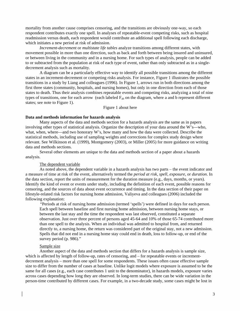
a measure of time at risk of the event, alternatively termed the period at risk, spell, exposure, or duration. In the data section, report the units of measurement for the duration measure (e.g., days, months, or years). Identify the kind of event or events under study, including the definition of each event, possible reasons for censoring, and the sources of data about event occurrence and timing. In the data section of their paper on lifestyle-related risk factors for nursing home admission, Valiyeva and colleagues (2006) included the following explanation:

“Periods at risk of nursing home admission (termed ‘spells’) were defined in days for each person. Each spell between baseline and first nursing home admission, between nursing home stays, or between the last stay and the time the respondent was last observed, constituted a separate observation. Just over three percent of persons aged 45-64 and 10% of those 65-74 contributed more than one spell to the analysis. When an individual was admitted to hospital from, and returned directly to, a nursing home, the return was considered part of the original stay, not a new admission. Spells that did not end in a nursing home stay could end in death, loss to follow-up, or end of the survey period (p. 986).”

Sample size Another aspect of the data and methods section that differs for a hazards analysis is sample size,

which is affected by length of follow-up, rates of censoring, and – for repeatable events or increment-decrement analysis – more than one spell for some respondents. These issues often cause effective sample size to differ from the number of cases at baseline. Unlike logit models where exposure is assumed to be the same for all cases (e.g., each case contributes 1 unit to the denominator), in hazards models, exposure varies across cases depending how long they are observed. In long-term studies, there can be wide variation in the person-time contributed by different cases. For example, in a two-decade study, some cases might be lost in

3

the first few months due to mortality, moving away, or other reasons, while other cases might contribute as many as 20 person-years of observation. See Yamaguchi (1991) for an excellent review of questions to consider when constructing your data set and calculating periods at risk.

As noted earlier, hazard rates for each time interval are based on person-time at risk in that interval. In studies with long follow-up periods and high rates of attrition or event occurrence, the population at risk at later time points can be substantially smaller than the population at baseline. In multivariate models, this problem is compounded because hazard rates are calculated for subgroups.

The following sections describe sample size and event information to report in the data section for each type of hazards analysis.

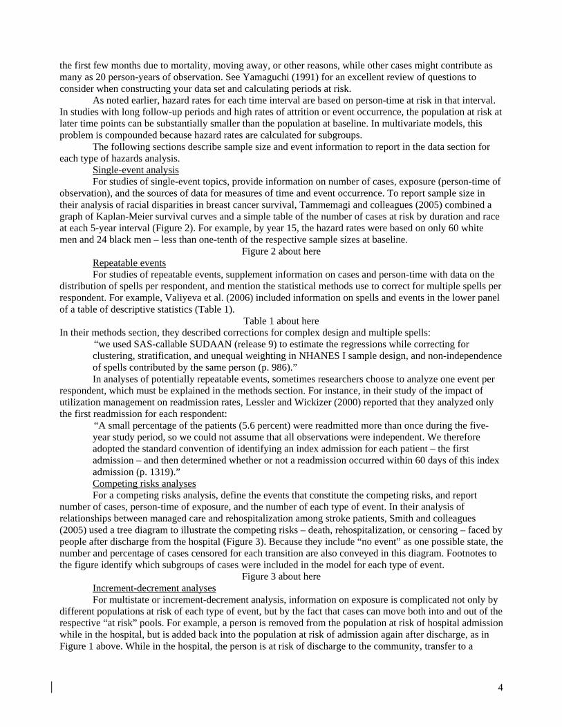
Single-event analysis For studies of single-event topics, provide information on number of cases, exposure (person-time of

observation), and the sources of data for measures of time and event occurrence. To report sample size in their analysis of racial disparities in breast cancer survival, Tammemagi and colleagues (2005) combined a graph of Kaplan-Meier survival curves and a simple table of the number of cases at risk by duration and race at each 5-year interval (Figure 2). For example, by year 15, the hazard rates were based on only 60 white men and 24 black men – less than one-tenth of the respective sample sizes at baseline.

Figure 2 about here Repeatable events For studies of repeatable events, supplement information on cases and person-time with data on the

distribution of spells per respondent, and mention the statistical methods use to correct for multiple spells per respondent. For example, Valiyeva et al. (2006) included information on spells and events in the lower panel of a table of descriptive statistics (Table 1).

Table 1 about here In their methods section, they described corrections for complex design and multiple spells:

“we used SAS-callable SUDAAN (release 9) to estimate the regressions while correcting for clustering, stratification, and unequal weighting in NHANES I sample design, and non-independence of spells contributed by the same person (p. 986).” In analyses of potentially repeatable events, sometimes researchers choose to analyze one event per

respondent, which must be explained in the methods section. For instance, in their study of the impact of utilization management on readmission rates, Lessler and Wickizer (2000) reported that they analyzed only the first readmission for each respondent:

“A small percentage of the patients (5.6 percent) were readmitted more than once during the five-year study period, so we could not assume that all observations were independent. We therefore adopted the standard convention of identifying an index admission for each patient – the first admission – and then determined whether or not a readmission occurred within 60 days of this index admission (p. 1319).” Competing risks analyses For a competing risks analysis, define the events that constitute the competing risks, and report

number of cases, person-time of exposure, and the number of each type of event. In their analysis of relationships between managed care and rehospitalization among stroke patients, Smith and colleagues (2005) used a tree diagram to illustrate the competing risks – death, rehospitalization, or censoring – faced by people after discharge from the hospital (Figure 3). Because they include “no event” as one possible state, the number and percentage of cases censored for each transition are also conveyed in this diagram. Footnotes to the figure identify which subgroups of cases were included in the model for each type of event.

Figure 3 about here Increment-decrement analyses For multistate or increment-decrement analysis, information on exposure is complicated not only by

different populations at risk of each type of event, but by the fact that cases can move both into and out of the respective “at risk” pools. For example, a person is removed from the population at risk of hospital admission while in the hospital, but is added back into the population at risk of admission again after discharge, as in Figure 1 above. While in the hospital, the person is at risk of discharge to the community, transfer to a

4

nursing home, or death. For an increment-decrement analysis, define the transitions to be studied, the number of each type of transition, and the number of cases and person-time at risk.

Independent variables In a hazards analysis, the element of time introduces another dimension not only to the dependent

variable, but to independent (explanatory) variables as well. Some independent variables will be fixed (also known as non-time-varying or time-invariant covariates), maintaining the same value throughout the observation period for a given case. The most obvious examples are variables such as gender and race, which cannot change. Other variables may be specified as fixed because they are only measured once even though they could change over time. For example, Lee and colleagues (1993) included baseline measures of body mass index, smoking, and exercise patterns as independent variables in their analysis of body weight and mortality. Definitions and statistics for fixed covariates can be presented as in other multivariate analyses.

Some independent variables may be specified as time-varying covariates (also known as time-dependent covariates, not to be confused with time-dependent effects; see below) if more than one measurement is available for a given case. In the data and methods section, identify time-varying independent variables, indicate the dates of or intervals between the repeated measurements, and mention the source of data for those variables. In their analysis of survival of AIDS patients treated and not treated with zidovudine, Lundgren and colleagues (1994) captured patients’ changing medication status as follows:

“Time since initiation of zidovudine was fitted in a Cox proportional hazards model as three time-dependent categories of time since starting zidovudine (<12 months, 12 to 24 months, and >24 months) and a category of never having received zidovudine (p. 1089).” For variables that could change over time but are specified as fixed, explain why (e.g., only one

measurement was available for each respondent), and return in the discussion section to consider implications for the interpretation of findings.

Model specification To explain your model specification, begin by indicating whether your model is specified as a

continuous-time hazards model, such as a Cox proportional hazards model or some types of parametric models, or as a discrete-time model such as a logistic hazards specification (Allison 1995; Yamaguchi 1991). Mention the independent variables, differentiating between key independent variable(s) and control variables in both text and tables.

Describe exploratory analyses used to arrive at your final model specification, including diagnostics to evaluate proportionality of hazards. Graphs of hazard rates by subgroup can be invaluable for illustrating situations where the assumption of proportionality is not met. For example, in a study of factors related to inpatient length of stay for youths with serious mental illness, Pottick and colleagues (1999) found that hazard rates of discharge for publicly and privately insured children were far from proportional (parallel) – they actually crossed one another quite steeply (Figure 4).

Figure 4 about here Although they did not include the figure in their article, the authors summarized the bivariate pattern

and its consequences for model specification: “Exploratory analyses revealed that the relationship between type of insurance and rate of discharge varied across time: For the first three weeks after admission, the rate of discharge for patients with private insurance was lower than for those with other means of payment, after which privately insured patients were discharged faster. Hence all models that include insurance type also include an interaction between time less than 21 days and lack of private insurance (Pottick et al. 1999; p. 220).”

The results section for a hazards analysis As in any results section, tables are preferable for presenting detailed statistical results (e.g.,

descriptive statistics and estimated coefficients and inferential statistical test results), whereas charts are more effective for portraying the general shapes of patterns, such as survival curves for different subgroups or interactions among variables. In the accompanying prose, explain the size and shape of each association and interpret the findings with reference to the specific concepts under study (see examples below).

5

Effective tables and charts are self-contained, so readers can interpret the meaning of every number without consulting the text. In the title, convey the topics or questions addressed in that table or chart, naming each of the major components of the relationships illustrated. For tables or charts based on multivariate hazards results, mention the type of model, the event(s) modeled, and the concepts captured by the independent variables. In the row and column labels of a table, or axis labels and legend of a chart, show the identity and units or coding for every variable; replace acronyms or other abbreviated variable names with short phrases that readers can understand without referring to the text.

Poor title: “Hazards results with confidence intervals.” Comment: This title fails to convey the type of event being modeled, the sample under study, the independent variables, whether reported results are coefficients (log-relative hazards) or hazard ratios, or the width of the reported confidence intervals (95% CI are most common, but other widths are sometimes used).

Better title: “Relative risks of all-cause mortality among Harvard alumni, 1962/1966 through 1988, according to body mass index.” (Table 2, from Lee et al., 1993).

Comment: This title identifies the event (all-cause mortality), the measure of effect size (relative risks), the key independent variable (body mass index; BMI), and the “W’s” for the sample (Harvard alumni, 1962/66-1988). The type of inferential statistical information (95% CI) and the list of control variables are mentioned in the column headings and footnotes, respectively, while the definition and units for BMI are given in the row heading.

Table 2 about here In tables of multivariate results, create separate columns for each model, labeling each model with a

number (e.g., “Model I”) or name (e.g., “Age-adjusted” and “Multivariate”, as in Table 2). Column headings can also be used to identify different competing risks or models for different subgroups. See (Miller 2005) for additional guidelines on creating tables and charts to present multivariate results.

Univariate and stratified statistics As you write about bivariate or multivariate patterns, incorporate information about the concepts and

units of the variables, keeping the focus on your research question. Also describe direction and magnitude of each association instead of simply reporting statistical significance or merely stating that variables were correlated. Examples of sentences to report these statistics are given below. See (Miller 2005) for more suggestions on how to describe statistical results.

Use tables of univariate and bivariate tables to report unadjusted levels and rates of event occurrence so that readers can assess their level and compare those values with data from other sources. Descriptive statistics on the independent variables can often be combined in a table with information on number of spells, person-years at risk, and so forth, as in Table 1 above. Relationships among independent variables can also be shown in tabular form, helping to make the case why a multivariate specification is needed to control for potential confounders. In their analysis of zidovudine and AIDS mortality, Lundgren and colleagues (1994) presented results of log-rank tests for the relationships between several other independent variables and initiation of zidovudine treatment (Table 3).

Table 3 about here Poor description: “The log-rank for year of AIDS diagnosis = 1988 showed that p =0.06, whereas for 1987 it was p<0.001”

Comment: Although this description reports statistical test results, it doesn’t mention that the log-rank test was testing for differences in chances of starting zidovudine, and fails to indicate which years had greater rates of zidovudine use.

Better description: “Fewer patients diagnosed [with AIDS] in 1987 received zidovudine compared with more recent years (Lundgren et al. 1994, p. 1090).”

Comment: This description incorporates the concepts (year and zidovudine use), and conveys the direction of association.

Univariate and stratified (e.g., bivariate) survival, cumulative failure, and hazard statistics are often best presented graphically because the key point is the general shape of those patterns rather than precise numeric values. For example, Figure 2 portrays survival curves from breast cancer, stratified by race

6

(Tammemagi et al. 2005). The p-value from the log-rank test (0.003; reported on the lower left-hand portion of the chart) demonstrates that differences across racial strata are statistically significant. Median survival time for each group is the time at which the proportion surviving drops below 0.5. If the level and shape of the hazard curve across time is of interest, consider including a graph – either of the hazard curve for all groups combined, or stratified by subgroup as in Figure 4.

Multivariate model results In most ways, tables of multivariate results from a hazards model are similar to tables of logistic

regression results. Accompany or replace coefficients (log-relative hazards) with hazard ratios. For categorical independent variables, present the hazard ratios in a table, then express the size in terms of multiples of risk compared to the reference category, which you name in the sentence. For continuous independent variables, report the hazard ratios in a table, then contrast other increments if a one-unit increase is not typical or of interest. Indicate statistical significance of each coefficient using confidence intervals (converted to the same units as hazard ratios; see comment under “hazard ratio” in Appendix for formula), p-values, or symbols or formatting to denote level of significance.

One key independent variable Table 2 above shows how to present hazard ratios for a single key predictor in the analysis – in this

case, body mass index (BMI) in a study of mortality (Lee et al. 1993). Other variables in their “multivariate” model are listed in a footnote to the table. Number of deaths, subjects, and person-years of exposure for each BMI subgroup are included in the table with the multivariate results.

Poor description: “In the age-adjusted model, the relative risk (RR) for BMI 23.5-24.5 was 0.96 (95% confidence interval (CI) 0.86, 1.06). [Paragraph continues with separate sentences for the RR and CI for each of the other three BMI groups, followed by parallel reporting of the RR and CI for the multivariate model.]”

Comment: This description essentially replicates the table contents without interpreting the shape of the relationship or naming the dependent variable.

Better description: “Taking into account age alone, we observed a J-shaped relation between BMI and all-cause mortality (Table 2) (p for linear trend = 0.02; p for quadratic trend = 0.003). The lowest mortality was in men with a BMI of 23.5 to less than 24.5. Men in the heaviest fifth of BMI (26.0 or greater) experienced a significantly higher risk of dying during follow-up than men in the lightest fifth (less than 22.5) (RR, 1.12, 95% CI, 1.03 to 1.22) (Lee et al. 1993, p. 2825).”

Comment: The authors start by naming the model to be described (“age alone”), the independent variable (BMI) and dependent variable (all-cause mortality), and using a simile (“J-shaped”) to describe the general shape of the relationship. They then identify the lowest and highest risk groups, the reference category (“lightest fifth”), and report the size and statistical significance of mortality differences between those groups.

They go on to explain: “When we further adjusted for cigarette smoking habit and physical activity, we again found the lowest mortality among men with a BMI of 23.5 to 24.5. Increased mortality risk among the heaviest fifth now was accentuated somewhat (RR, 1.18, 95% CI, 1.08 to 1.28; Lee et al. 1993, p. 2825).”

Comment: Rather than describing the entire shape of the BMI/mortality relationship again for their full multivariate model, the authors name that model (“further adjusted for…”) and use the word “again” to get across similarity of results with those in the previous model. In the second sentence, the phrase “accentuated somewhat” conveys that the mortality difference across BMI groups was slightly larger than in the age-adjusted one.

Charts can also be used to report adjusted results for a key independent variable. On the same tree diagram that they use to illustrate competing risks, Smith and colleagues (2005) report adjusted hazard ratios comparing the risk of each type of transition for HMO versus fee-for-service, associated 95% CIs, and number of cases for each type of transition (see Figure 3 above).

Lessler and Wickizer (2000) use a cumulative failure chart to show the relationship between length of stay (LOS) reductions due to prospective utilization management and risk of subsequent readmission (Figure 5). They accompany the chart with the following description:

7

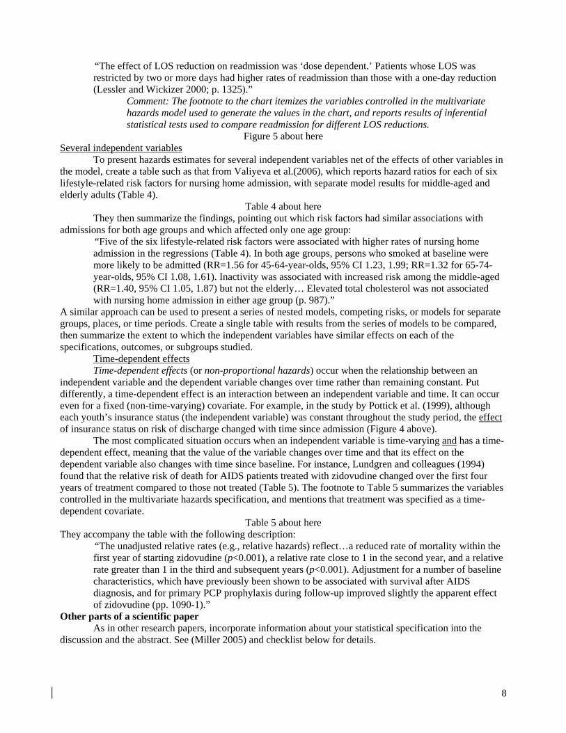
“The effect of LOS reduction on readmission was ‘dose dependent.’ Patients whose LOS was restricted by two or more days had higher rates of readmission than those with a one-day reduction (Lessler and Wickizer 2000; p. 1325).”

Comment: The footnote to the chart itemizes the variables controlled in the multivariate hazards model used to generate the values in the chart, and reports results of inferential statistical tests used to compare readmission for different LOS reductions.

Figure 5 about here Several independent variables

To present hazards estimates for several independent variables net of the effects of other variables in the model, create a table such as that from Valiyeva et al.(2006), which reports hazard ratios for each of six lifestyle-related risk factors for nursing home admission, with separate model results for middle-aged and elderly adults (Table 4).

Table 4 about here They then summarize the findings, pointing out which risk factors had similar associations with

admissions for both age groups and which affected only one age group: “Five of the six lifestyle-related risk factors were associated with higher rates of nursing home admission in the regressions (Table 4). In both age groups, persons who smoked at baseline were more likely to be admitted (RR=1.56 for 45-64-year-olds, 95% CI 1.23, 1.99; RR=1.32 for 65-74-year-olds, 95% CI 1.08, 1.61). Inactivity was associated with increased risk among the middle-aged (RR=1.40, 95% CI 1.05, 1.87) but not the elderly… Elevated total cholesterol was not associated with nursing home admission in either age group (p. 987).”

A similar approach can be used to present a series of nested models, competing risks, or models for separate groups, places, or time periods. Create a single table with results from the series of models to be compared, then summarize the extent to which the independent variables have similar effects on each of the specifications, outcomes, or subgroups studied.

Time-dependent effects Time-dependent effects (or non-proportional hazards) occur when the relationship between an

independent variable and the dependent variable changes over time rather than remaining constant. Put differently, a time-dependent effect is an interaction between an independent variable and time. It can occur even for a fixed (non-time-varying) covariate. For example, in the study by Pottick et al. (1999), although each youth’s insurance status (the independent variable) was constant throughout the study period, the effect of insurance status on risk of discharge changed with time since admission (Figure 4 above).

The most complicated situation occurs when an independent variable is time-varying and has a time-dependent effect, meaning that the value of the variable changes over time and that its effect on the dependent variable also changes with time since baseline. For instance, Lundgren and colleagues (1994) found that the relative risk of death for AIDS patients treated with zidovudine changed over the first four years of treatment compared to those not treated (Table 5). The footnote to Table 5 summarizes the variables controlled in the multivariate hazards specification, and mentions that treatment was specified as a time-dependent covariate.

Table 5 about here They accompany the table with the following description:

“The unadjusted relative rates (e.g., relative hazards) reflect…a reduced rate of mortality within the first year of starting zidovudine (p<0.001), a relative rate close to 1 in the second year, and a relative rate greater than 1 in the third and subsequent years (p<0.001). Adjustment for a number of baseline characteristics, which have previously been shown to be associated with survival after AIDS diagnosis, and for primary PCP prophylaxis during follow-up improved slightly the apparent effect of zidovudine (pp. 1090-1).”

Other parts of a scientific paper As in other research papers, incorporate information about your statistical specification into the

discussion and the abstract. See (Miller 2005) and checklist below for details.

8

Summary Writing about hazards analysis shares many aspects with writing about other types of multivariate

models, including the basic contents of the data and methods sections, and use of tables, charts, and prose to present statistical results as evidence for the research question at hand. However, the focus on not only occurrence but time to events such as mortality also requires reporting information related to measurement of the temporal aspects of the dependent and independent variables and sample size, as well as the type of hazards model specification. By following the guidelines and examples in this paper, authors can improve the completeness and clarity of their papers on applications of survival analysis to topics in health and health services research.

Checklist In the abstract: • Under methods, name the type of hazards model used in your analysis, the number of cases, and the

length of follow-up. • Under results, summarize key findings about relative hazards and cumulative failure or survival. In the data section: • Set the context for your study (the W’s: who, when, where) • Define your independent variable:

o Indicate what event(s) you are studying and whether they are One-time or repeatable One-way or increment-decrement Competing risks, and if so, the specific types of competing events

o Explain what constitutes censoring in your data • Specify the maximum possible length of the follow-up and dates or intervals of follow-up. • Mention the data sources that provided information on event occurrence and timing. • Report the following aspects of sample size

o Number of cases (respondents) o Person-time at risk, including units of time.

• For repeated events, report: o Number of spells o Number or percentage of cases with more than one spell o Corrections for multiple observations per case.

• Define your independent variables, indicating o Which are fixed (time-invariant) o Which are time-varying, and how often were they measured.

In the methods section: • Name the type of statistical specification (e.g., Cox proportional hazards model). • Explain how you arrived at your model specification, including diagnostics for proportionality and other

exploratory data analysis. In the results section: • Use tables to present detailed statistical findings, charts to show general patterns.

o Make each table or chart self-contained, naming the concepts, types of statistics, context (W’s), and the identity and units or coding of every variable. o Report direction, magnitude, and statistical significance of associations between variables, explaining time-dependent effects, if any.

In the discussion and conclusions • Describe advantages of hazards models for your specific research question and data. • Discuss limitations of your data such as single measures of potentially time-varying covariates or sources

of data on event occurrence and timing.

9

Literature cited Allison, P.D., 1995. Survival Analysis Using the SAS System: A Practical Guide. Cary, NC: SAS Institute. Cox, D.R., and D. Oakes, 1984. Analysis of Survival Data. Monographs on Statistics and Applied

Probability. New York: Chapman and Hall. Kalbfleisch, J.D. and R.L. Prentice, 1980. The Statistical Analysis of Failure Time Data. New York: John

Wiley and Sons, Inc. Lee, I-M, J.E. Manson, C.H. Hennekens, and R.S. Paffenbarger, 1993. "Body Weight and Mortality: A 27-

year Follow-up of Middle-aged Men," Journal of the American Medical Association. 270(23):2823-8. Lessler, D.S., and T.M. Wickizer, 2000. “The Impact of Utilization Management on Readmissions among

Patients with Cardiovascular Disease,” Health Services Research. 34(6):1315-1329. Liang, J., X. Liu, E. Tu, and N. Whitelaw, 1996. “Probabilities and Lifetime Durations of Short-stay Hospital

and Nursing Home Use in the United States, 1985,” Medical Care. 34(10):1018-1036. Lundgren, J.D., A.N. Phillips, C. Pedersen, N. Cluneck, J.M. Gatell, A.M. Johnson, B. Ledergerber, S. Vella

and J.O. Nielsen, 1994. "Comparison of Long-term Prognosis of Patients with AIDS Treated and Not Treated with Zidovudine," Journal of the American Medical Association. 271(14):1088-92.

Maciejewski, M.L., P. Diehr, M.A. Smith, and P. Hebert. 2002. “Common Methodological Terms in Health Services Research and their Symptoms.” Medical Care. 40: 477–84.

Miller, J.E. 2005. The Chicago Guide to Writing about Multivariate Analysis. Chicago: University of Chicago Press.

Montgomery, S.L. 2003. The Chicago Guide to Communicating Science. Chicago: University of Chicago Press.

Pottick, K.J., S. Hansell, J.E. Miller and D. Davis, 1999. “Factors Associated with Inpatient Length of Stay for Children and Adolescents with Serious Mental Illness.” Social Work Research. 23(4):213-24.

Smith, M.A., J.R. Frytak, J-I. Liou, and M.D. Finch, 2005. “Rehospitalization and Survival for Stroke Patients in Managed Care and Traditional Medicare Plans,” Medical Care. 43(9):902-910.

Tammemagi, C.M., D. Nerenz, C. Neslund-Dudas, C. Feldkamp, and D. Nathanson, 2005. “Comorbidity and Survival Disparities among Black and White Patients with Breast Cancer,” Journal of the American Medical Association. 294(14):1765-1772.

Wilkinson, Leland, and Task Force on Statistical Inference, APA Board of Scientific Affairs. 1999. “Statistical Methods in Psychology Journals: Guidelines and Explanations.” American Psychologist. 54 (8): 594–604.

Yamaguchi, K., 1991. Event History Analysis. Applied Social Research Methods Series, Volume 28. Newbury Park, California: Sage Publications.

Valiyeva, E., L.B. Russell, J.E. Miller, and M. Safford, 2006. “Lifestyle-related Risk Factors and Risk of Nursing Home Admission,” Archives of Internal Medicine.166:985-990

Acknowledgements: I would like to thank Deborah Carr, Louise Russell, and Cynthia Fontanella for helpful comments on earlier drafts of this manuscript.

10

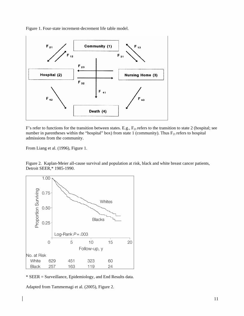
Figure 1. Four-state increment-decrement life table model.

F’s refer to functions for the transition between states. E.g., F21 refers to the transition to state 2 (hospital; see number in parentheses within the “hospital” box) from state 1 (community). Thus F21 refers to hospital admissions from the community. From Liang et al. (1996), Figure 1. Figure 2. Kaplan-Meier all-cause survival and population at risk, black and white breast cancer patients, Detroit SEER,* 1985-1990.

* SEER = Surveillance, Epidemiology, and End Results data. Adapted from Tammemagi et al. (2005), Figure 2.

11

Figure 3. Adjusted hazards ratios (HRs) and 95% confidence intervals (95% CI) for the relationship between membership in HMO (n=4,816) versus fee-for-service (FFS; n=4,187) and death or hospitalization, sample of U.S. Medicare beneficiaries, 1988-2000.

Adjusted for female, race, age, Medicaid, % of census block group aged 25 or older with college degrees, % of census block living below the poverty line, geographic region, previous health conditions (see Smith et al., p. 906) and year of index hospitalization. ** p <0.05 † Model includes 176 patients who died after being hospitalized. ‡ Model includes 728 patients with no 30-day event who died after being rehospitalized. § Model includes 209 patients who were rehospitalized during the first 30 days and were rehospitalized again and subsequently died during the subsequent 11 months. Adapted from Smith et al. (2005), Figure 1.

12

Figure 4: Hazard of discharge by type of insurance and duration, 1986 U.S. C/PSS youth sample*

0.000

0.010

0.020

0.030

0.040

0.050

0.060

0 7 14 21 28 35 42 49 56 63

Time since admission (days)

Wee

kly

haza

rd o

f dis

char

ge

private public

*C/PSS = Client/Patient Sample Survey; youths are <18 years of age at time of admission. Data from Pottick et al. (1999), personal communication. Figure 5. Sixty-day readmission rates among patients with cardiovascular disease initially admitted for a procedure, by reduction in LOS during initial admission, 1989-1993 (n = 993)

The lines shown in Figure 5 represent the cumulative readmission risk adjusted for: age, sex, geographic region, total days requested, catheterization requested, year of request, and total number of reviews performed. The relative risk of 60-day readmission was statistically significant for LOS reduction of 2+ days compared to reduction of 0 days (RR = 2.6; p < 0.005), but not for a LOS restriction of one day. Adapted from Lessler and Wickizer (2000), Figure 1.

13

Appendix. Terminology for hazards models

Terms and synonyms Definition

Example topics,

exhibits, and citations* Comments

General terminology for hazards models

Hazards analysis

Survival analysis

Event history analysis

Cox regression Failure time analysis

Life table modeling Duration analysis

Type of statistical analysis used to study patterns and correlates of event occurrence and timing.

Mortality Hospital admission

Event

Transition Failure Source of decrement

When a case moves from one state to another. Each type of transition is one kind of event.

Transition from alive to dead (Lundgren et al. 1994)

Discharge from hospital to community (Pottick et al. 1999)

Measured with a categorical variable indicating change from one discrete state to another. See “event indicator.”

Event indicator Categorical variable used to specify the status of a case at the end of a spell. One component of the dependent variable in a hazards model.

Binary: 1 = event occurred; 0 = censored

Multichotomous: 1 = hospital admission; 2 = nursing home admission; 3 = death; 0 = censored (Liang et al. 1996)

Can be binary (dichotomous) or multichotomous.

Spell

Period at risk

Duration Exposure

Length of time since start of observation period or time at risk. Second component of the dependent variable in a hazards model.

Years from baseline to death

Days from hospital discharge to readmission (Lessler and Wickizer 2000)

For repeatable events, each respondent can contribute more than one spell.

Population at risk

Cohort

The group of cases that could potentially experience the event as of start of observation period.

For hospital admission: Persons living in the community or a nursing home

For hospital discharge: Persons in the hospital (Liang et al. 1996)

Population at risk depends on type of event (see examples)

Censoring When the event is not observed for a given spell.

Loss-to-follow-up

Dropping out of study End of observation period

without event Mortality (for studies of

events other than death)

Includes both those who have not yet and those who may never experience the event.

Reasons for censoring depend on the type of event and data source(s).

Survival When the event has not yet occurred for a given case.

For mortality: Remaining alive

For hospital admission: Not yet having been admitted to the hospital

For topics other than mortality, “survival” refers to not yet having experienced the event.

Survival curve Chart showing the proportion of the cohort (population at risk) that has not yet experienced the event, plotted against time since baseline.

Proportion of breast cancer patients surviving, by years since diagnosis (Figure 2)

Survival = 1 – cumulative failure.

Starts at 1.0. Can only decline or remain level, cannot increase.

Can be stratified to show patterns for subgroups.

Cumulative failure curve Chart showing the proportion of the cohort (population at risk) that has experienced the event, plotted against time since baseline.

For study of readmission: Proportion readmitted, by time since last discharge (Figure 5)

Cumulative failure = 1.0 – survival.

Starts at 0. Can only increase or remain level, cannot decrease.

Can be stratified to show patterns for subgroups.

Hazard rate

Transition rate

Rate of event occurrence within a time interval, conditional on survival to the beginning of that time interval.

Weekly rate of hospital discharge, by type of insurance (Figure 4)

Number of events within a time interval divided by person-time at risk in that time interval.

Can be stratified to show patterns for subgroups.

Hazard ratio

Relative hazard

For categorical independent variables, the relative risk of event occurrence in a category of interest compared to the reference category.

For continuous independent variables, the relative risk of event occurrence associated with a 1-unit increase in that independent variable.

Relative risk of all-cause mortality for BMI ≥ 26.0 versus BMI <22.5 (Table 2)

Hazard ratio = eβ = exp(β), where β = the coefficient from a hazards model. Hence the coefficient is the log-relative-hazard.

Confidence limits for a hazard ratio are calculated exp(β ± [1.96 × standard error]).

Hazards models for different types of events

Single-decrement model Type of hazards model used to analyze a single type of event.

All-cause mortality (Lee et al. 1993)

Contrast against a competing risks model.

Repeatable event model Type of hazards model used to analyze events that can occur more than once to each respondent.

Nursing home admission (Valiyeva et al. 2006)

Can be single- or multiple-decrement.

Competing risks model

Multiple-decrement model

Type of hazards model used to analyze several alternative, mutually exclusive types of events.

Multiple causes of death, e.g., heart disease vs. cancer vs. all other causes

Rehospitalization vs. mortality (Figure 3)

Contrast against a single-decrement model.

Can be one-way or increment-decrement.

Increment-decrement model

Multistate life table

Type of hazards model used to analyze reversible transitions or transitions among several different states or conditions.

Reversible transition: Insurance status (insured to uninsured)

Multistate: Transitions among community, hospitals, nursing homes, and death (Figure 1)

Can be single-decrement or competing risks model.

Time dependence in hazards models†

Cox proportional hazards model

Proportional hazards model

Type of hazards model where the hazard ratio for two subgroups is constant over the period of observation.

Relationship between body mass index and mortality (Lee et al. 1993).

A type of semi-parametric hazards model.

Non-proportional hazards

Time-dependent effects

Type of hazards model where the hazard ratio for two subgroups changes during the period of observation.

Mortality rate for patients treated with a medication is initially lower than that for untreated patients, but the relationship is reversed later in the observation period (Lundgren et al. 1994).

Specified as an interaction between an independent variable and time since baseline.

Can be specified with semi-parametric or parametric model.

Can occur for fixed or time-varying covariates.

Fixed covariate

Non-time-varying covariate

Time-invariant covariate

An independent (explanatory) variable whose value remains the same throughout the spell.

Gender

Weight at baseline (Lee et al. 1993)

Some variables that could theoretically change across time may be defined as fixed because of data constraints.

Time-varying covariate

Time-dependent covariate

An independent variable whose value changes during the spell.

Smoking status

Medication regimen during study period (Lundgren et al. 1994)

Requires repeated observations or longitudinal surveillance data.

Can, but does not necessarily, have a time-dependent effect on risk of event occurrence.

* Tables and figures cited refer to those in the body of the article. See list of references for full citations. † See Allison (1995) or Yamaguchi (1991) for information on other functional forms for hazards models, including discrete-time and parametric hazards models. See Cox and Oakes (1984), Allison (1995), or Yamaguchi (1991) for an in-depth discussion of concepts and terms for hazards analysis.

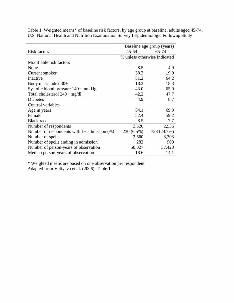
Table 1. Weighted means* of baseline risk factors, by age group at baseline, adults aged 45-74,

U.S. National Health and Nutrition Examination Survey I Epidemiologic Followup Study

Risk factor/

Baseline age group (years)

45-64 65-74

% unless otherwise indicated

Modifiable risk factors

None 8.5 4.9

Current smoker 38.2 19.0

Inactive 51.2 64.2

Body mass index 30+ 18.3 18.3

Systolic blood pressure 140+ mm Hg 43.0 65.9

Total cholesterol 240+ mg/dl 42.2 47.7

Diabetes 4.9 8.7

Control variables

Age in years 54.1 69.0

Female 52.4 59.2

Black race 8.5 7.7

Number of respondents 3,526 2,936

Number of respondents with 1+ admission (%) 230 (6.5%) 728 (24.7%)

Number of spells

3,660 3,303

Number of spells ending in admission 282 900

Number of person-years of observation 58,027 37,420

Median person-years of observation 18.6 14.1

* Weighted means are based on one observation per respondent.

Adapted from Valiyeva et al. (2006), Table 1.

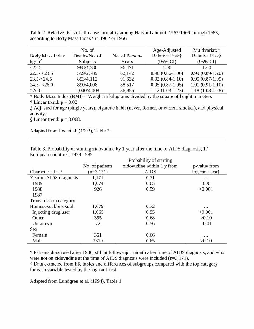
Table 2. Relative risks of all-cause mortality among Harvard alumni, 1962/1966 through 1988,

according to Body Mass Index* in 1962 or 1966.

Body Mass Index

kg/m2

No. of

Deaths/No. of

Subjects

No. of Person-

Years

Age-Adjusted

Relative Risk†

(95% CI)

Multivariate‡

Relative Risk§

(95% CI)

<22.5 988/4,380 96,471 1.00 1.00

22.5- <23.5 599/2,789 62,142 0.96 (0.86-1.06) 0.99 (0.89-1.20)

23.5-<24.5 853/4,112 91,632 0.92 (0.84-1.10) 0.95 (0.87-1.05)

24.5- <26.0 890/4,008 88,517 0.95 (0.87-1.05) 1.01 (0.91-1.10)

≥26.0 1,040/4,008 86,956 1.12 (1.03-1.23) 1.18 (1.08-1.28)

* Body Mass Index (BMI) = Weight in kilograms divided by the square of height in meters

† Linear trend: p = 0.02

‡ Adjusted for age (single years), cigarette habit (never, former, or current smoker), and physical

activity.

§ Linear trend: p = 0.008.

Adapted from Lee et al. (1993), Table 2.

Table 3. Probability of starting zidovudine by 1 year after the time of AIDS diagnosis, 17

European countries, 1979-1989

Characteristics*

No. of patients

(n=3,171)

Probability of starting

zidovudine within 1 y from

AIDS

p-value from

log-rank test†

Year of AIDS diagnosis 1,171 0.71 …

1989 1,074 0.65 0.06

1988 926 0.59 <0.001

1987

Transmission category

Homosexual/bisexual 1,679 0.72 …

Injecting drug user 1,065 0.55 <0.001

Other 355 0.68 >0.10

Unknown 72 0.56 =0.01

Sex

Female 361 0.66 …

Male 2810 0.65 >0.10

* Patients diagnosed after 1986, still at follow-up 1 month after time of AIDS diagnosis, and who

were not on zidovudine at the time of AIDS diagnosis were included (n=3,171).

† Data extracted from life tables and differences of subgroups compared with the top category

for each variable tested by the log-rank test.

Adapted from Lundgren et al. (1994), Table 1.

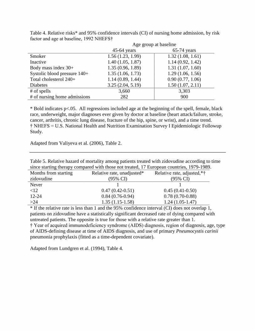
Table 4. Relative risks* and 95% confidence intervals (CI) of nursing home admission, by risk

factor and age at baseline, 1992 NHEFS†

Age group at baseline

45-64 years 65-74 years

Smoker 1.56 (1.23, 1.99) 1.32 (1.08, 1.61)

Inactive 1.40 (1.05, 1.87) 1.14 (0.92, 1.42)

Body mass index 30+ 1.35 (0.96, 1.89) 1.31 (1.07, 1.60)

Systolic blood pressure 140+ 1.35 (1.06, 1.73) 1.29 (1.06, 1.56)

Total cholesterol 240+ 1.14 (0.89, 1.44) 0.90 (0.77, 1.06)

Diabetes 3.25 (2.04, 5.19) 1.50 (1.07, 2.11)

# of spells 3,660 3,303

# of nursing home admissions 282 900

* Bold indicates p<.05. All regressions included age at the beginning of the spell, female, black

race, underweight, major diagnoses ever given by doctor at baseline (heart attack/failure, stroke,

cancer, arthritis, chronic lung disease, fracture of the hip, spine, or wrist), and a time trend.

† NHEFS = U.S. National Health and Nutrition Examination Survey I Epidemiologic Followup

Study.

Adapted from Valiyeva et al. (2006), Table 2.

Table 5. Relative hazard of mortality among patients treated with zidovudine according to time

since starting therapy compared with those not treated, 17 European countries, 1979-1989.

Months from starting

zidovudine

Relative rate, unadjusted*

(95% CI)

Relative rate, adjusted,*†

(95% CI)

Never 1 1

<12 0.47 (0.42-0.51) 0.45 (0.41-0.50)

12-24 0.84 (0.76-0.94) 0.78 (0.70-0.88)

>24 1.35 (1.15-1.58) 1.24 (1.05-1.47)

* If the relative rate is less than 1 and the 95% confidence interval (CI) does not overlap 1,

patients on zidovudine have a statistically significant decreased rate of dying compared with

untreated patients. The opposite is true for those with a relative rate greater than 1.

† Year of acquired immunodeficiency syndrome (AIDS) diagnosis, region of diagnosis, age, type

of AIDS-defining disease at time of AIDS diagnosis, and use of primary Pneumocystis carinii

pneumonia prophylaxis (fitted as a time-dependent covariate).

Adapted from Lundgren et al. (1994), Table 4.