Embed Size (px)
Citation preview
STATA May 1994
TECHNICAL STB-19
BULLETINA publication to promote communication among Stata users
Editor Associate Editors
Sean Becketti J. Theodore Anagnoson, Cal. State Univ., LAStata Technical Bulletin Richard DeLeon, San Francisco State Univ.8 Wakeman Road Paul Geiger, USC School of MedicineSouth Salem, New York 10590 Lawrence C. Hamilton, Univ. of New Hampshire914-533-2278 Stewart West, Baylor College of Medicine914-533-2902 [email protected] EMAIL
Subscriptions are available from Stata Corporation, email [email protected], telephone 979-696-4600 or 800-STATAPC,fax 979-696-4601. Current subscription prices are posted at www.stata.com/bookstore/stb.html.
Previous Issues are available individually from StataCorp. See www.stata.com/bookstore/stbj.html for details.
Submissions to the STB, including submissions to the supporting files (programs, datasets, and help files), are ona nonexclusive, free-use basis. In particular, the author grants to StataCorp the nonexclusive right to copyright anddistribute the material in accordance with the Copyright Statement below. The author also grants to StataCorp the rightto freely use the ideas, including communication of the ideas to other parties, even if the material is never publishedin the STB. Submissions should be addressed to the Editor. Submission guidelines can be obtained from either theeditor or StataCorp.
Copyright Statement. The Stata Technical Bulletin (STB) and the contents of the supporting files (programs,datasets, and help files) are copyright c by StataCorp. The contents of the supporting files (programs, datasets, andhelp files), may be copied or reproduced by any means whatsoever, in whole or in part, as long as any copy orreproduction includes attribution to both (1) the author and (2) the STB.
The insertions appearing in the STB may be copied or reproduced as printed copies, in whole or in part, as longas any copy or reproduction includes attribution to both (1) the author and (2) the STB. Written permission must beobtained from Stata Corporation if you wish to make electronic copies of the insertions.
Users of any of the software, ideas, data, or other materials published in the STB or the supporting files understandthat such use is made without warranty of any kind, either by the STB, the author, or Stata Corporation. In particular,there is no warranty of fitness of purpose or merchantability, nor for special, incidental, or consequential damages suchas loss of profits. The purpose of the STB is to promote free communication among Stata users.
The Stata Technical Bulletin (ISSN 1097-8879) is published six times per year by Stata Corporation. Stata is a registeredtrademark of Stata Corporation.
Contents of this issue page
an42. STB-13—STB-18 available in bound format 2an43. New address for STB office 2an44. StataQuest: Stata for teaching 3an45. Stata and Stage now available for DEC Alpha 4
dm17. Conversions for international date formats 4dm18. Adding trailing moving averages to the egen command 5gr14. dotplot: Comparative scatterplots 8gr15. Incorporating Stata graphs in TEX documents using an HP printer 11os12. Windowed interfaces for Stata 14os13. Using awk and fgrep for selective extraction from Stata log files 15
sg22.3. Generalized linear models: revision of glm. Rejoinder 17sqv9. Probit coefficients as changes in probabilities 17ssa3. Adjusted survival curves 22ssa4. Ex post tests and diagnostics for a proportional hazards model 23ssa5. Note on time intervals in time-varying Cox regression 28
ssi5.3. Correction to Ridders’ method 28sts7.2. A library of time series programs for Stata (Update) 28zz3.3. Computerized index for the STB (Update) 30
zz4. Cumulative index for STB-13—STB-18 31
2 Stata Technical Bulletin STB-19
an1.1 STB categories and insert codes
Inserts in the STB are presently categorized as follows:
General Categories:an announcements ip instruction on programmingcc communications & letters os operating system, hardware, &dm data management interprogram communicationdt data sets qs questions and suggestionsgr graphics tt teachingin instruction zz not elsewhere classified
Statistical Categories:sbe biostatistics & epidemiology srd robust methods & statistical diagnosticssed exploratory data analysis ssa survival analysissg general statistics ssi simulation & random numberssmv multivariate analysis sss social science & psychometricssnp nonparametric methods sts time-series, econometricssqc quality control sxd experimental designsqv analysis of qualitative variables szz not elsewhere classified
In addition, we have granted one other prefix, crc, to the manufacturers of Stata for their exclusive use.
an42 STB-13—STB-18 available in bound format
Sean Becketti, Stata Technical Bulletin, FAX 914-533-2902
The third year of the Stata Technical Bulletin (issues 13–18) has been reprinted in a 240+ page bound book called The StataTechnical Bulletin Reprints, Volume 3. The volume of reprints is available from StataCorp for $25—$20 for STB subscribers—plusshipping. Authors of inserts in STB-13—STB-18 will automatically receive the book at no charge and need not order.
This book of reprints includes everything that appeared in issues 13–18 of the STB. As a consequence, you do not needto purchase the reprints if you saved your STBs. However, many subscribers find the reprints useful since they are bound in avolume that matches the Stata manuals in size and appearance. Our primary reason for reprinting the STB, though, is to make iteasier and cheaper for new users to obtain back issues. For those not purchasing the reprints, note that zz4 in this issue providesa cumulative index for the third year of the original STBs.
an43 New address for STB office
Sean Becketti, Stata Technical Bulletin, FAX 914-533-2902
The editorial office of the STB has moved from Kansas to New York. Submissions and other correspondence should be sentto
Sean Becketti, EditorStata Technical Bulletin8 Wakeman RoadSouth Salem, New York 10590914-533-2278 (voice)914-533-2902 (FAX)
Please note that this address is only for matters related to the STB. Questions about ordering Stata products (including the STB)or other questions about Stata should be directed to
Stata Corporation702 University Drive EastCollege Station, Texas 77840409-696-4600 (voice)409-696-4601 (FAX)
Direct technical support for individually supported users is also available directly from StataCorp by telephone, FAX, or mail.U.S. and Canadian users may call the toll-free number, 800-STATAPC. Have your Stata serial number handy so the support staffcan quickly identify the version of Stata you are using.
Stata Technical Bulletin 3
an44 StataQuest: Stata for teaching
Stan Loll, Editor, Statistical Computing, Duxbury Press, 415-637-7596, email stan [email protected]
I am pleased to announce a new version of Stata for teaching undergraduate statistics, StataQuest.
Duxbury Press, an imprint of Wadsworth Publishing Company, publishes college textbooks exclusively in statistics and suchassociated fields as operations research, decision sciences, and quality control. Our list includes Statistics with Stata 3 (Hamilton1993). About a year ago, we contracted with Stata Corporation to develop a special version of Stata for the undergraduateintroductory statistics market. Our requirements were
1. The program should be 100% compatible with professional Stata, minus the advanced statistical topics (logistic regression,factor analysis, etc.)
2. The program would fit on and run from a single floppy diskette.
3. The program would look and work the same on both MS DOS and Macintosh computers.
4. The program would be easy enough for the average computerphobic freshman to use with little or nor help from theinstructor. This meant that the program needed to be completely menu driven with a clear, consistent interface.
5. The program would contain a context-sensitive help system.
6. The program would have a fully integrated spreadsheet data editor for easy data entry and examination .
7. The program would include all necessary functions for the first course in statistics.
8. Duxbury would be able to offer the program at a very attractive price.
The program is now finished and is called StataQuest. A DOS or Macintosh StataQuest diskette is included with this issue ofthe STB for those who subscribe with magnetic media. (If you subscribe with Unix media, the DOS version of StataQuest isincluded; no Unix version of StataQuest exists yet. Look for the Unix version of StataQuest next year.)
DOS users insert the diskette into the A drive and, from the A>: prompt, type go.
Macintosh users insert the diskette, double-click to open the diskette icon, and then double-click on StataQuest.
In addition to the StataQuest software, Duxbury commissioned Ted Anagnoson and Rich DeLeon to write the text StataQuest(253 pp.)—which accompanies the software when it is purchased independently—and the StataQuest Text Companion (65pp.)—which accompanies the software when it is purchased with other Duxbury and Wadsworth titles.
The StataQuest text covers the essentials of setting up, inputting, analyzing, and presenting data at the beginning andintermediate levels; the book with software sells for $18 and is available both from Duxbury and Stata Corporation. Examinationcopies are available through your usual Duxbury representative.
The shorter StataQuest Text Companion, on the other hand, cannot be purchased separately (although examination copies areavailable). This book-plus-software combination is made available at low, low cost to adopters of other Duxbury and Wadsworthtitles. Under this plan, students can receive a Duxbury/Wadsworth text, the Text Companion, and the StataQuest software all forlittle more than the cost of the Duxbury/Wadsworth text alone.
The 253-page StataQuest User’s Guide contains
1. Research and data analysis with StataQuest: Steps in conducting research. A working vocabulary for data analysis. Statistical versus graphicsmethods. Exploratory and confirmatory approaches. A StataQuest tutorial. Appendix: Questions about StataQuest. How do I :::?
2. Basics of using microcomputers and StataQuest: What StataQuest is. Hardware basics. Operating systems. StataQuest compared with other versionsof Stata. StataQuest basics. Questions and problems. Appendix: Analyzing subsets of data.
3. Files: Open. Save. Import ASCII. Export ASCII. Session logging. Maintenance Quit. Maximum size of StataQuest datafiles. Questions and problems.
4. StataQuest spreadsheet: Starting StataQuest’s spreadsheet. How the spreadsheet works. Moving from cell to cell. How to input new data. Correctingmistakes. Changing the data. Sorting the data. Labels. Saving the file. Appendix: Additional StataQuest functions.
5. Graphs, part 1: Creating StataQuest graphs: the graphs submenu. Graphs of one variable. Graphs of one variable by groups. Comparison graphsof different variables.
6. Graphs, part 2: Scatter plots. Time series plots. Quality control charts.
4 Stata Technical Bulletin STB-19
7. Summaries: Simple data analysis: Describe the data. Means and standard deviations. Confidence intervals. List the data. Data detail (medians,:::). Tables.
8. Parametric and nonparametric tests: Parametric tests. Nonparametric tests. Questions and problems.
9. Correlation, simple regression, and robust regression: A brief introduction to correlation and regression. Pearson and Spearman correlationcoefficients. Simple regression. Robust regression.
10. Multiple regression: Multiple regression (regular). Multiple regression (stepwise).
11. Analysis of variance (ANOVA): Nonparametric analysis of variance. One-way ANOVA. Two-way ANOVA. Two-way factorial ANOVA. Morecomplex ANOVA. Questions and problems.
12. The statistical calculator: Confidence interval for the mean. Student’s t-test (one-sample). Student’s t-test (two-sample). Standard deviation tests.Binomial probability test. Poisson confidence interval. On-line statistical tables. The expression evaluator—a personal calculator. Questions andproblems.
The 65-page Text Companion contains
1. Getting started: Preview. StataQuest’s menu and submenu commands. Getting started.
2. Files: Open. Save. Import ASCII. Export ASCII. Session logging. Maintenance. Quit.
3. Edit/spreadsheet: Activating and using the spreadsheet. Menus. Moving the cursor. Files. Add. Drop. Replace. Sort. Label. Useful command-modeoptions.
4. Graphs: One variable. One variable by groups. Comparison of variables. Scatter plots. Time series. Quality Control. View saved graphs.
5. Summaries: Describe data. Means and standard deviations. Confidence intervals. List data. Data detail (medians, :::). Tables.
6. Statistics: Parametric tests. Nonparametric tests. Correlation. Simple regression. Multiple regression. Robust regression. ANOVA.
7. Calculator: Confidence interval for mean. Student’s t-test (one sample). Student’s t-test (two sample). Standard deviation tests. Binomial probabilitytest. Binomial confidence interval. Poisson confidence interval. On-line statistical tables. Expression evaluator.
We at Duxbury are very excited about StataQuest and have extensive plans for continuing StataQuest development. For moreinformation, contract your local Duxbury/Wadsworth representative or give me a call. I would appreciate receiving you commentson StataQuest.
[Also see comments by Gould in os12 for a different aspect of StataQuest—Ed.]
ReferencesAnagnoson, J. T. and R. E. DeLeon. 1994a. StataQuest. Belmont, CA: Duxbury Press.
——. 1994b. StataQuest Text Companion. Belmont, CA: Duxbury Press.
Hamilton, L. C. 1993. Statistics with Stata 3. Belmont, CA: Duxbury Press.
an45 Stata and Stage now available for DEC Alpha
Tim McGuire, Stata Corporation, FAX 409-696-4601
Stata 3.1 and the Stata Graphics Editor (Stage) are now available for the DEC Alpha running OSF/1 (Unix). The DEC Alphais a 64-bit workstation with a true 64-bit operating system. If you’ve followed the computer press, you know that the Alpha isa very fast machine. Moreover, the Alpha supports Unix (in the form of OSF/1) and the X Window standard.
Stata 3.1 on the DEC Alpha, is like Stata 3.1 on all other platforms; thus version 3.1 data sets, graphs, and ado-files fromother computers can be used without translation. Pricing is the same as for all Stata/Unix systems.
dm17 Conversions for international date formats
Philip Ryan, University of Adelaide, Department of Community MedicineFAX (011)-61-8-223-4075, EMAIL [email protected]
For those of us living outside the United States, it is sometimes an irritation that software written in the U.S. pays littleattention to date formats used by other countries. We Stata users are fortunate that Stata has such a rich set of date formatconverters (especially after the publication of jtoe.ado and etoj.ado in STB-14). The built-in Stata commands ftodate anddatetof handle conversions to and from numerical formatted dates of the form yymmdd and strings of the form “mm/dd/yy”.However, Stata does not provide a means of converting between formatted dates and strings of the form “dd/mm/yy”. Forexample, in many countries the date November 14, 1993 is represented by “14/11/93” and not, as in the U.S., by “11/14/93”. Adate such as “11/30/93” would be read by an American as November 30, 1993, but would be nonsense elsewhere as there is no30th month of the year.
Stata Technical Bulletin 5
To rectify this situation, I have altered the code of ftodate and datetof to produce two new commands, ftoidateand idatetof. The “i” is meant to suggest “international.” The new commands handle a new string variable type, idatevar,containing “dd/mm/yy”. The syntax of these commands is
idatetof idatevar�if exp
� �in range
�, generate(fvar)
ftoidate fvar�if exp
� �in range
�, generate(idatevar)
It would be somewhat presumptuous of me to claim any credit for this, as all I have done is alter the order of output fromStata’s original ftodate and datetof commands. However, others using Stata outside the U.S. may find the new commandshelpful.
ReferencesBecketti S. 1993. dm14.1: Converting Stata elapsed dates to Julian dates. Stata Technical Bulletin 14: 10.
Chapin C. 1993. dm14: Converting Julian dates to Stata elapsed dates. Stata Technical Bulletin 14: 8–10.
dm18 Adding trailing moving averages to the egen command
Sean Becketti, Stata Technical Bulletin, FAX 914-533-2902
The egen command provides a host of useful extensions to generate. These extensions are typically functions not currentlyavailable as built-in Stata functions; that is, they are functions that cannot be used in general Stata expressions. Examples includefunctions to calculate means, medians, percentiles, ranks, and other statistics, often within levels of grouping variables. A moreunusual example is the diff(varlist) function which generates an indicator variable equal to 1 when all the variables in varlist areequal. All the functions in egen could be replaced either by short sequences of built-in Stata commands or by separate ado-filesfor each function. Thus, egen is a housekeeping device: it provides convenient access to a variety of data transformations whileavoiding the proliferation of commands that would result from coding these transformations as separate ado-files.
egen is constructed to make it easy to add new features. For instance, StataCorp added the group() function in STB-12.More recently, Schmidt (1993) added a function to calculate marginal U.S. income tax rates. This insert adds yet another function,the trailing moving average, and explains how you can add your own data transformations to egen.
tma(): trailing moving averages
A trailing moving average of span s is the moving average of the current observation of a variable along with the precedings� 1 observations. For example, if x is a Stata variable, the 4-period (span 4) trailing moving average of x can be created bytyping
. generate y = (x + x[_n-1] + x[_n-2] + x[_n-3])/4
The syntax of tma(), the trailing moving average extension to egen, is
egen�type
�newvar = tma(exp)
�if exp
� �in range
� �, nomiss span(#) notaper
�Options
nomiss indicates that newvar should be missing whenever any of the observations in the averaging span are missing. By default,tma() returns the average of the nonmissing observations in the span as long as there is at least one nonmissing observation.
span(#) specifies the span of the moving average. If no span is specified, tma() tries to determine the periodicity of the databy calling the period program from Stata’s time series library. (See sts7.2 in this issue for a discussion of the time serieslibrary.) If this call is successful, tma() sets the span to the periodicity of the data, that is, 4 for quarterly data, 12 formonthly data, and so on. If the period program is not found, the span is set to 3.
notaper prevents the calculation of moving averages at the beginning of the series where less than s values are available. Bydefault, tma() tapers the beginning of the moving average. For example, if you type egen y=tma(x), span(4), the firstfour values of y are calculated as
6 Stata Technical Bulletin STB-19
y[1] = x[1]
y[2] = (x[1] + x[2])=2
y[3] = (x[1] + x[2] + x[3])=3
y[4] = (x[1] + x[2] + x[3] + x[4])=4
Comparison with ma(), the centered moving average
egen already provides a centered moving average function, ma(), but this function has some inconvenient restrictions. First,because ma() generates centered moving averages, it only accepts odd spans (specified by the t() option). Even spans—4 forquarterly data, 12 for monthly data, etc.—are much more common in time series analysis, though. tma() allows any positivespan.
ma() treats the endpoints of the series differently than does tma(). By default, ma() behaves as though the notaper optionof tma() was specified. ma()’s nomiss option (which is different from tma()’s nomiss option) allows tapering, but both thebeginning and ending of the series are tapered. There is no need to taper the end of the series in a trailing moving average.
Finally, ma() generates missing values whenever any observation in the span is missing. tma() normally averages whatevernonmissing observations are available. tma()’s nomiss option replicates ma()’s treatment of missing observations.
Having both tma() and ma() raises some questions of program design. First, the names of similar options and their defaultsettings differ between the two functions. Normally, I would try to avoid these differences. In this case, the option names anddefaults for tma() were chosen to reflect the spirit of other, general smoothers (see, for example [5s] smooth), and I thought itmore important to give tma() a “natural” syntax than to make it conform to ma()’s design.
Second, it is a bit confusing to have two functions that perform such similar tasks. It would take very little effort to combinetma() and ma() into a single function that calculates both types of moving averages. I thought it best, though, to publish tma()
and get some initial feedback from users before making this sort of change.
Examples
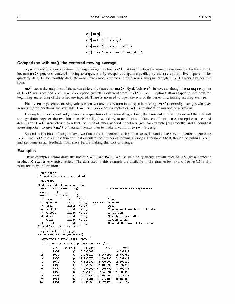
These examples demonstrate the use of tma() and ma(). We use data on quarterly growth rates of U.S. gross domesticproduct, G.gdp, a very noisy series. (The data used in this example are available in the time series library. See sts7.2 in thisissue for more information.)
. use money
(Growth rates for regression)
. describe
Contains data from money.dta
Obs: 133 (max= 32766) Growth rates for regression
Vars: 8 (max= 99)
Width: 28 (max= 200)
1. year int %8.0g Year
2. quarter int %8.0g quarter Quarter
3. date float %9.0g Date
4. D.rtb3 float %9.0g Change in 3-month T-bill rate
5. G.defl float %9.0g Inflation
6. G.gdp float %9.0g Growth of real GDP
7. G.m2 float %9.0g Growth of M2
8. rqual float %9.0g 6-month CP minus T-bill rate
Sorted by: year quarter
. egen cma3 = ma(G.gdp)
(2 missing values generated)
. egen tma3 = tma(G.gdp), span(3)
. list year quarter G.gdp cma3 tma3 in f/10
year quarter G.gdp cma3 tma3
1. 1959 Q2 6.787582 . 6.787582
2. 1959 Q3 -1.385613 2.564982 2.700985
3. 1959 Q4 2.292975 2.684199 2.564981
4. 1960 Q1 7.145234 2.794885 2.684199
5. 1960 Q2 -1.053553 2.165739 2.794885
6. 1960 Q3 .4055356 -1.069926 2.165739
7. 1960 Q4 -2.56176 .3849031 -1.069926
8. 1961 Q1 3.310934 2.164368 .3849031
9. 1961 Q2 5.743931 4.945139 2.164368
10. 1961 Q3 5.780552 6.520123 4.945139

Stata Technical Bulletin 7
. list year quarter G.gdp cma3 tma3 in -5/l
year quarter G.gdp cma3 tma3
129. 1991 Q2 1.697554 -.0551785 -1.80077
130. 1991 Q3 1.218768 1.156871 -.0551785
131. 1991 Q4 .5542907 1.557511 1.156871
132. 1992 Q1 2.899475 1.661858 1.557511
133. 1992 Q2 1.531807 . 1.661858
This example shows the default tapering used by tma() (which is different, by the way, from the odd-span-only taperingavailable with ma()’s nomiss option). In the middle of the run, a 3-span ma() is just a lagged version of a 3-span tma(). (A5-span ma() is a twice-lagged version, and so on.) Since tma() is trailing looking, there are no missing values at the end ofthe series.
In the example above, I specified the span(3) option with tma(). Because I keep the time series library in my adopath,tma() would have used a default span of 1 because the period command returns a period of 1 if no period has been set. Sincethese data are quarterly, it makes sense to use period to let other programs know that four periods make a natural grouping.
. period 4
4 (quarterly)
. egen tma4 = tma(G.gdp)
. list year quarter G.gdp tma3 tma4 in f/10
year quarter G.gdp tma3 tma4
1. 1959 Q2 6.787582 6.787582 6.787582
2. 1959 Q3 -1.385613 2.700985 2.700985
3. 1959 Q4 2.292975 2.564981 2.564981
4. 1960 Q1 7.145234 2.684199 3.710045
5. 1960 Q2 -1.053553 2.794885 1.749761
6. 1960 Q3 .4055356 2.165739 2.197548
7. 1960 Q4 -2.56176 -1.069926 .9838639
8. 1961 Q1 3.310934 .3849031 .0252889
9. 1961 Q2 5.743931 2.164368 1.72466
10. 1961 Q3 5.780552 4.945139 3.068414
Adding your own functions to egen()
Most Stata users accumulate a collection of special-purpose do-files and ado-files that perform frequently used datatransformations. egen is designed to make it easy to convert these transformations into new egen functions. By attaching yourspecial functions to egen, you make it easier to share these functions with your coauthors and colleagues while simultaneouslyreducing the proliferation of small, limited-purpose ado-files.
egen actually does very little. It guarantees that newvar is a legal new variable, then calls the ado-file for the specifiedfunction to do all the work. By convention, the ado-file for a function called, say, xxx, is gxxx.ado.
Let’s use tma() as an example to clarify the process. In the example above, I calculated trailing moving averages of span 3by typing
egen tma3 = tma(G.gdp), span(3)
After a bit of parsing, egen issued the command:
gtma tma3 G.gdp, span(3)
My program for trailing moving averages, gtma.ado begins with the lines
*! _gtma -- trailings moving average for egen (STB-19: dm18)
*! version 1.0.0 Sean Becketti March 1994
program define _gtma
quietly fversion 3.1
local varlist "req new max(1)"
local exp "req nopre"
local if "opt"
local in "opt"
local options "noMiss Span(integer 0) noTaper"
parse "`*'"
8 Stata Technical Bulletin STB-19
The program expects to receive a new variable, an expression (without an “=” prefix), and, perhaps, if and in clauses, andsome options. After parsing these, the program proceeds to the calculations, which are straightforward in this case.
Extensions to egen can be more elaborate than tma(). Several of the functions, for example, take a varlist rather than anexpression as their argument. Any conceivable set of arguments can be specified. egen simply passes them to your ado-file forprocessing.
To add your function to egen, just store your ado-file somewhere in the adopath, so egen can find it. If your ado-filedetects an error, simply exit with a non-zero return code (using either the exit # or error # command), and egen will cleanup the mess. Additional tips on linking to egen are listed at the bottom of the file egen.ado.
ReferencesSchmidt, T. 1993. ss1: Calculating U.S. marginal tax rates. Stata Technical Bulletin 15: 17–19.
Stata Corporation. 1993. crc27: More extensions to generate: categorical variables. Stata Technical Bulletin 12: 3–4.
gr14 dotplot: Comparative scatterplots
Peter Sasieni, Imperial Cancer Research Fund, London, FAX (011)-44-71-269 3429Patrick Royston, Royal Postgraduate Medical School, London, FAX (011)-44-81-740 3119
dotplot.ado produces a figure that is a cross between a boxplot, a histogram and a scatterplot. Like a boxplot, it ismost useful for comparing the distributions of several variables or the distribution of a single variable in several groups. Like ahistogram, the figure provides a crude estimate of the density and, as with a scatterplot, each symbol (dot) represents a singleobservation.
Syntax
dotplot varname�if exp
� �in range
� �, by(groupvar) nx(#) ny(#)
centre average(string) bar exact y graph options�
– or –
dotplot varlist�if exp
� �in range
� �, nx(#) ny(#)
centre average(string) bar exact y graph options�
Description
A dotplot is a scatterplot with a grouping of values in the vertical direction (“binning,” as in a histogram), and withseparation between plotted points in the horizontal direction. The aim is to display all the data for several variables or groupsin a single, compact graphic.
In the first form, dotplot produces a columnar dotplot of varname, with one column per value of groupvar. In the secondform, dotplot produces a columnar dotplot for each variable in varlist, with one column per variable; by(groupvar) is notallowed. In each case, the “dots” are plotted as small circles to increase readability.
If the data set was sorted before using dotplot, the program will prompt the user to press the F4 key to restore the originalorder.
Options
nx(#) sets the horizontal dot density. A larger value of # will increase the dot density, reducing the horizontal separation betweendots. This will increase the separation between columns if two or more groups or variables are used. The value of nx isstored in $S 1.
ny(#) sets the vertical dot density (number of “bins” on the y-axis). A larger value of # will result in more bins and a plotwhich is less spread-out in the horizontal direction. # should be determined in conjunction with nx() to give the mostpleasing appearance. The value of ny is stored in $S 2.
Stata Technical Bulletin 9
centre centres the dots for each column around a hidden vertical line.
average(string) plots a horizontal line of pluses at the average of each group. The string specifies whether the average shouldbe the mean or the median.
bar plots horizontal dashed lines at the “shoulders” of each group. The “shoulders” are taken to be the upper and lower quartilesunless average(mean) has been specified in which case they will be the mean plus or minus the standard deviation.
exact y uses the actual values of yvar rather than grouping them. This may be useful if yvar only takes on a few values; thatis, if yvar is a discrete variable.
graph options are any of the standard Stata twoway graph options except xscale(). If you use the symbol() option, note thatdotplot plots the dots, the average, the lower bar, and the upper bar in that order. If a single symbol is provided by theuser, it will be used for the dots and the default symbols will be used for the average and bars. If two or more symbolsare provided, they will be followed by the “plus”, “dash”, “dash”. Thus s(do) average(median) bar will use diamondsfor the data, small circles for the median, pluses for the lower quartile, and dashes for the upper quartile.
Examples
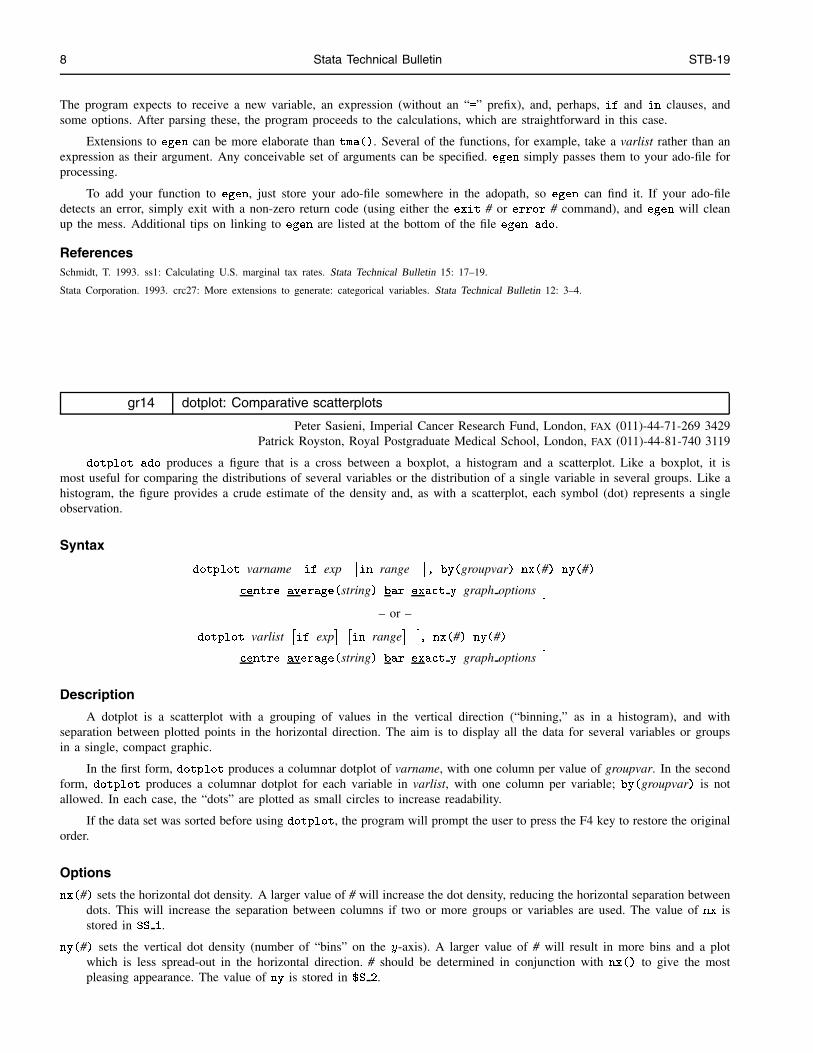
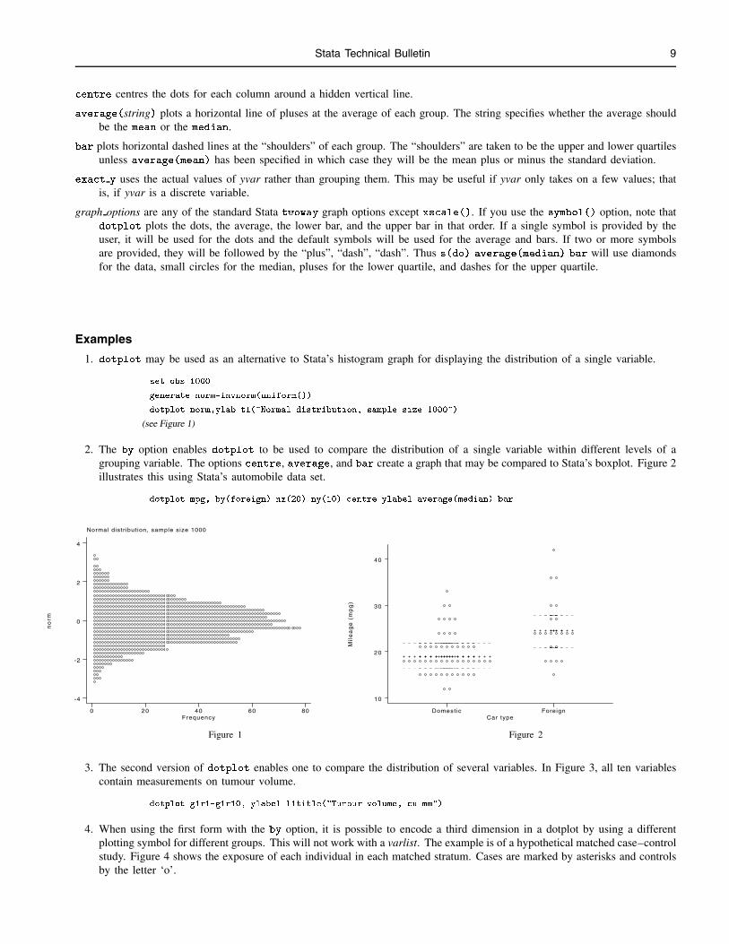
1. dotplot may be used as an alternative to Stata’s histogram graph for displaying the distribution of a single variable.
. set obs 1000
. generate norm=invnorm(uniform())
. dotplot norm,ylab t1("Normal distribution, sample size 1000")
(see Figure 1)
2. The by option enables dotplot to be used to compare the distribution of a single variable within different levels of agrouping variable. The options centre, average, and bar create a graph that may be compared to Stata’s boxplot. Figure 2illustrates this using Stata’s automobile data set.
. dotplot mpg, by(foreign) nx(20) ny(10) centre ylabel average(median) bar
Normal distr ibution, sample size 1000
no
rm
F requency0 20 40 60 80
-4
-2
0
2
4
Mil
ea
ge
(m
pg
)
Car typeDomest ic Foreign
10
20
30
40
_ __ _ _ _ _ _ _ _ _ _ __ _ _ _ _ _ _ _ _ _ _ _ _ _ _ _ __ _ _ _ _ _ _ _ _ _ __ _ _ __ _ _ __ __
__ _ _ __ __ _ _ _ _ _ _ __ __ __ ___ __ _ _ _ _ _ _ _ _ _ __ _ _ _ _ _ _ _ _ _ _ _ _ _ _ _ __ _ _ _ _ _ _ _ _ _ __ _ _ __ _ _ __ __
__ _ _ __ __ _ _ _ _ _ _ __ __ __ __
Figure 1 Figure 2
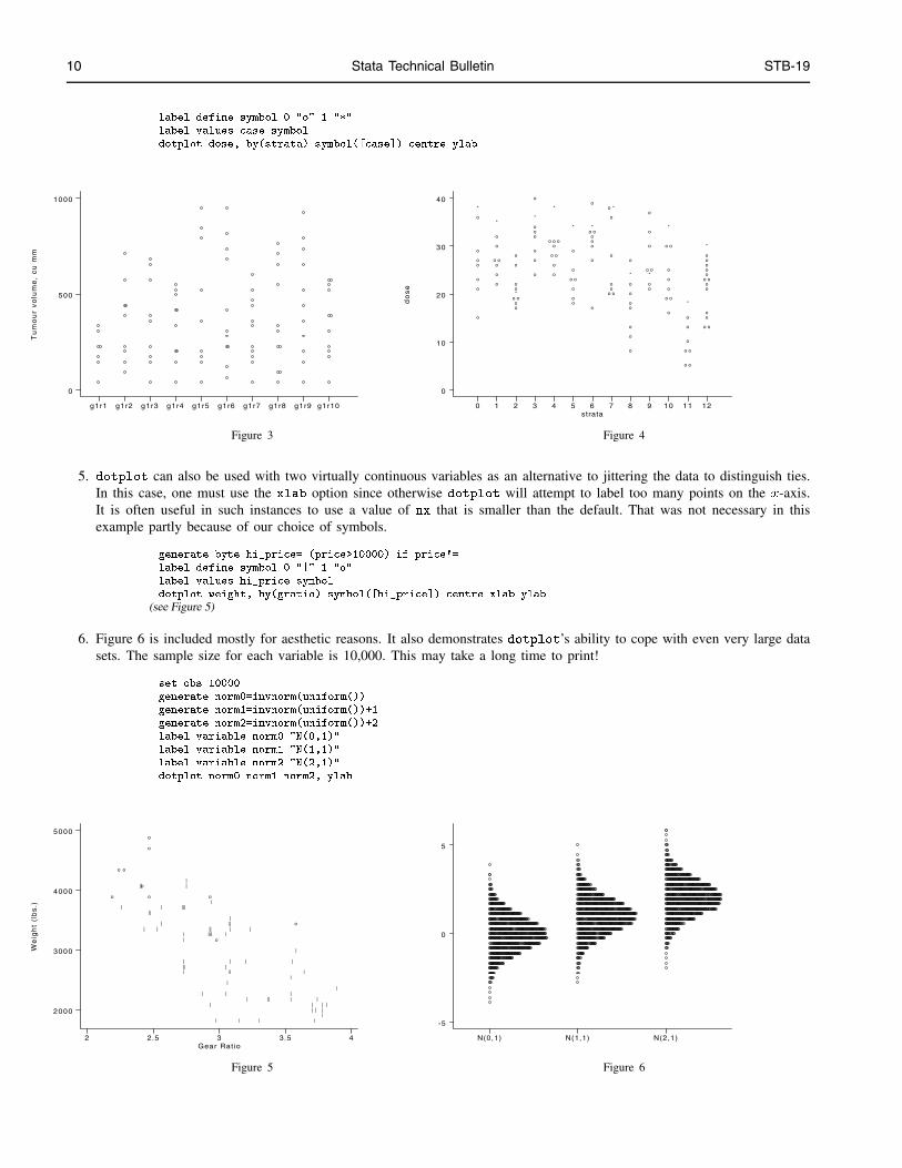
3. The second version of dotplot enables one to compare the distribution of several variables. In Figure 3, all ten variablescontain measurements on tumour volume.
. dotplot g1r1-g1r10, ylabel l1title("Tumour volume, cu mm")
4. When using the first form with the by option, it is possible to encode a third dimension in a dotplot by using a differentplotting symbol for different groups. This will not work with a varlist. The example is of a hypothetical matched case–controlstudy. Figure 4 shows the exposure of each individual in each matched stratum. Cases are marked by asterisks and controlsby the letter ‘o’.
10 Stata Technical Bulletin STB-19
. label define symbol 0 "o" 1 "*"
. label values case symbol
. dotplot dose, by(strata) symbol([case]) centre ylab
Tu
mo
ur
vo
lum
e,
cu
mm
g1r1 g1r2 g1r3 g1r4 g1r5 g1r6 g1r7 g1r8 g1r9 g1r10
0
500
1000
do
se
s trata9 1110 12852 710 4 63
0
10
20
30
40
o
o
o
oo
o
o
*
o
o
oo o
o
o
*
oo
o o*oo
o
o
o
o
o
ooo
*
o
o
o
o o
oo o o
*
oo
o
o o
o
o
*
o
o
ooo
o o*
o
o ooo
o
o
o *
o
o
o
oo
o
o
*
o
oo
*o o
o
o
o
o
o o
o
o
o
o o
*
o o
o o
o
o
o
*
o o
oo
oo
o oooooo
*
Figure 3 Figure 4
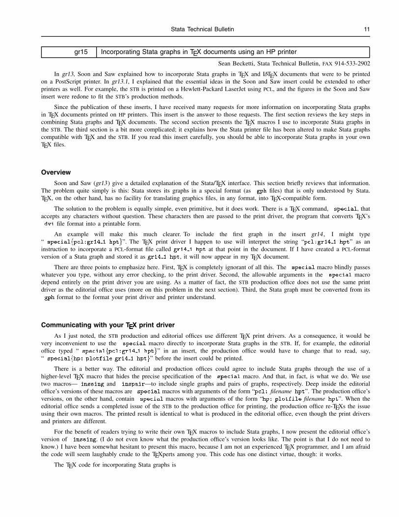
5. dotplot can also be used with two virtually continuous variables as an alternative to jittering the data to distinguish ties.In this case, one must use the xlab option since otherwise dotplot will attempt to label too many points on the x-axis.It is often useful in such instances to use a value of nx that is smaller than the default. That was not necessary in thisexample partly because of our choice of symbols.
. generate byte hi_price= (price>10000) if price!=.
. label define symbol 0 "|" 1 "o"
. label values hi_price symbol
. dotplot weight, by(gratio) symbol([hi_price]) centre xlab ylab
(see Figure 5)
6. Figure 6 is included mostly for aesthetic reasons. It also demonstrates dotplot’s ability to cope with even very large datasets. The sample size for each variable is 10,000. This may take a long time to print!
. set obs 10000
. generate norm0=invnorm(uniform())
. generate norm1=invnorm(uniform())+1
. generate norm2=invnorm(uniform())+2
. label variable norm0 "N(0,1)"
. label variable norm1 "N(1,1)"
. label variable norm2 "N(2,1)"
. dotplot norm0 norm1 norm2, ylab
We
igh
t (l
bs
.)
Gear Ratio2 2.5 3 3.5 4
2000
3000
4000
5000
o
o
|
o
||o
|
||
o
o
o
||
|
||||
||
|||
||
|
|
||||||
o|
|
o
|
|
|
|
||
|
||||
|
|
|
|
|
|| ||
|
|
|
o
|
||
|
|
|
||| |
|
N(0,1) N(1,1) N(2,1)
-5
0
5
Figure 5 Figure 6
Stata Technical Bulletin 11
gr15 Incorporating Stata graphs in TEX documents using an HP printer
Sean Becketti, Stata Technical Bulletin, FAX 914-533-2902
In gr13, Soon and Saw explained how to incorporate Stata graphs in TEX and LATEX documents that were to be printedon a PostScript printer. In gr13.1, I explained that the essential ideas in the Soon and Saw insert could be extended to otherprinters as well. For example, the STB is printed on a Hewlett-Packard LaserJet using PCL, and the figures in the Soon and Sawinsert were redone to fit the STB’s production methods.
Since the publication of these inserts, I have received many requests for more information on incorporating Stata graphsin TEX documents printed on HP printers. This insert is the answer to those requests. The first section reviews the key steps incombining Stata graphs and TEX documents. The second section presents the TEX macros I use to incorporate Stata graphs inthe STB. The third section is a bit more complicated; it explains how the Stata printer file has been altered to make Stata graphscompatible with TEX and the STB. If you read this insert carefully, you should be able to incorporate Stata graphs in your ownTEX files.
Overview
Soon and Saw (gr13) give a detailed explanation of the Stata/TEX interface. This section briefly reviews that information.The problem quite simply is this: Stata stores its graphs in a special format (as .gph files) that is only understood by Stata.TEX, on the other hand, has no facility for translating graphics files, in any format, into TEX-compatible form.
The solution to the problem is equally simple, even primitive, but it does work. There is a TEX command, \special, thataccepts any characters without question. These characters then are passed to the print driver, the program that converts TEX’s.dvi file format into a printable form.
An example will make this much clearer. To include the first graph in the insert gr14 , I might type“\specialfpcl:gr14 1.hptg”. The TEX print driver I happen to use will interpret the string “pcl:gr14 1.hpt” as aninstruction to incorporate a PCL-format file called gr14 1.hpt at that point in the document. If I have created a PCL-formatversion of a Stata graph and stored it as gr14 1.hpt, it will now appear in my TEX document.
There are three points to emphasize here. First, TEX is completely ignorant of all this. The \special macro blindly passeswhatever you type, without any error checking, to the print driver. Second, the allowable arguments in the \special macrodepend entirely on the print driver you are using. As a matter of fact, the STB production office does not use the same printdriver as the editorial office uses (more on this problem in the next section). Third, the Stata graph must be converted from its.gph format to the format your print driver and printer understand.
Communicating with your TEX print driver
As I just noted, the STB production and editorial offices use different TEX print drivers. As a consequence, it would bevery inconvenient to use the \special macro directly to incorporate Stata graphs in the STB. If, for example, the editorialoffice typed “\specialfpcl:gr14 1.hptg” in an insert, the production office would have to change that to read, say,“\specialfhp: plotfile gr14 1.hptg” before the insert could be printed.
There is a better way. The editorial and production offices could agree to include Stata graphs through the use of ahigher-level TEX macro that hides the precise specification of the \special macro. And that, in fact, is what we do. We usetwo macros—\inssing and \inspair—to include single graphs and pairs of graphs, respectively. Deep inside the editorialoffice’s versions of these macros are \special macros with arguments of the form “pcl: filename.hpt”. The production office’sversions, on the other hand, contain \special macros with arguments of the form “hp: plotfile filename.hpt”. When theeditorial office sends a completed issue of the STB to the production office for printing, the production office re-TEXs the issueusing their own macros. The printed result is identical to what is produced in the editorial office, even though the print driversand printers are different.
For the benefit of readers trying to write their own TEX macros to include Stata graphs, I now present the editorial office’sversion of \inssing. (I do not even know what the production office’s version looks like. The point is that I do not need toknow.) I have been somewhat hesitant to present this macro, because I am not an experienced TEX programmer, and I am afraidthe code will seem laughably crude to the TEXperts among you. This code has one distinct virtue, though: it works.
The TEX code for incorporating Stata graphs is

12 Stata Technical Bulletin STB-19
\def\inssing#1#2f\vboxf\centerpclf3.5ingf2.2ingf#1.hptg\vskip.2in
\centerlineff\smrmf#2ggggg
\inssing takes two arguments, the filename (excluding the filetype) of the Stata graph file and the title of the figure. The \smrm
macro is another of our private macros; it sets the title in the 8 point Computer Modern Roman font. You may replace it withany font command that suits you.
The \centerpcl macro allocates space for the Stata graph and inserts it in the document. This macro was supplied withmy copy of TEX. It reads as follows:
\def\centerpcl#1#2#3f\vskip#2\relax\centerlinef\hbox to#1f\specialfpcl:#3g\hfilggg
The crucial bit here is the \special macro. The rest of the macro makes sure the graph is placed in the correct location onthe page. The distances used—3.5 in and 2.2 in for arguments #1 and #2—were determined by trial and error.
Adapting Stata’s print driver
In the TEX macros above, a fixed amount of space is allowed for the Stata graph. For these macros to produce the desiredresult, the Stata graph must be stored in a PCL-format file and the PCL commands in that file must produce a graph of theexpected size.
The gphdot and gphpen programs convert Stata graphs from the .gph format to a printable form ([3] printing). For theSTB, we use gphdot because the HP LaserJet is a dot device. The following command was used to convert the graph displayedas Figure 1 in gr14:
gphdot gr14 1 /dtex /r52 /t14 /n
Four options modify the appearance of the graph. Taking them in reverse order, /n suppresses the Stata logo on the printedgraph. /t14 adjusts the thickness of the pens that draw various lines of the graph. Experimentation revealed that /t14 producesa graph that is easy to read at the size used in the STB. The graph is reduced to 52 percent of its normal size by the /r52 option.Finally, the /dtex option indicates that gphdot should use the printer file tex.dot when converting gr14 1.gph.
tex.dot is an adaptation of the hplphr.dot printer file that comes with Stata. hplphr.dot describes the HP LaserJet togphdot. The use of printer files allows StataCorp to add new printers quickly without changing the gphdot or gphpen programs.hplphr.dot and tex.dot are ordinary ASCII files. You can edit them, as we did, to make any needed adjustments.
Adapting the hplphr.dot is the one tricky part of the whole process. To make things as clear as possible, I’ve reproducedthe entire tex.dot below, and I’ve included tex.dot on the STB distribution diskette. There are only a few things you needto understand, so don’t get overwhelmed by this block of mysterious-looking code.
/*
STATA/GPH HP LaserJet+ Printer Configuration File
Copyright (C) 1986-1989, by ==C=R=C==
o 300 dots per inch (high-resolution) portrait aspect
(Requires 345K of PC memory to build graphic image)
NOTE: This configuration will NOT work on a regular LaserJet
(without the LaserJet PLUS features).
For release 2 STATA/GPHDOT
*/
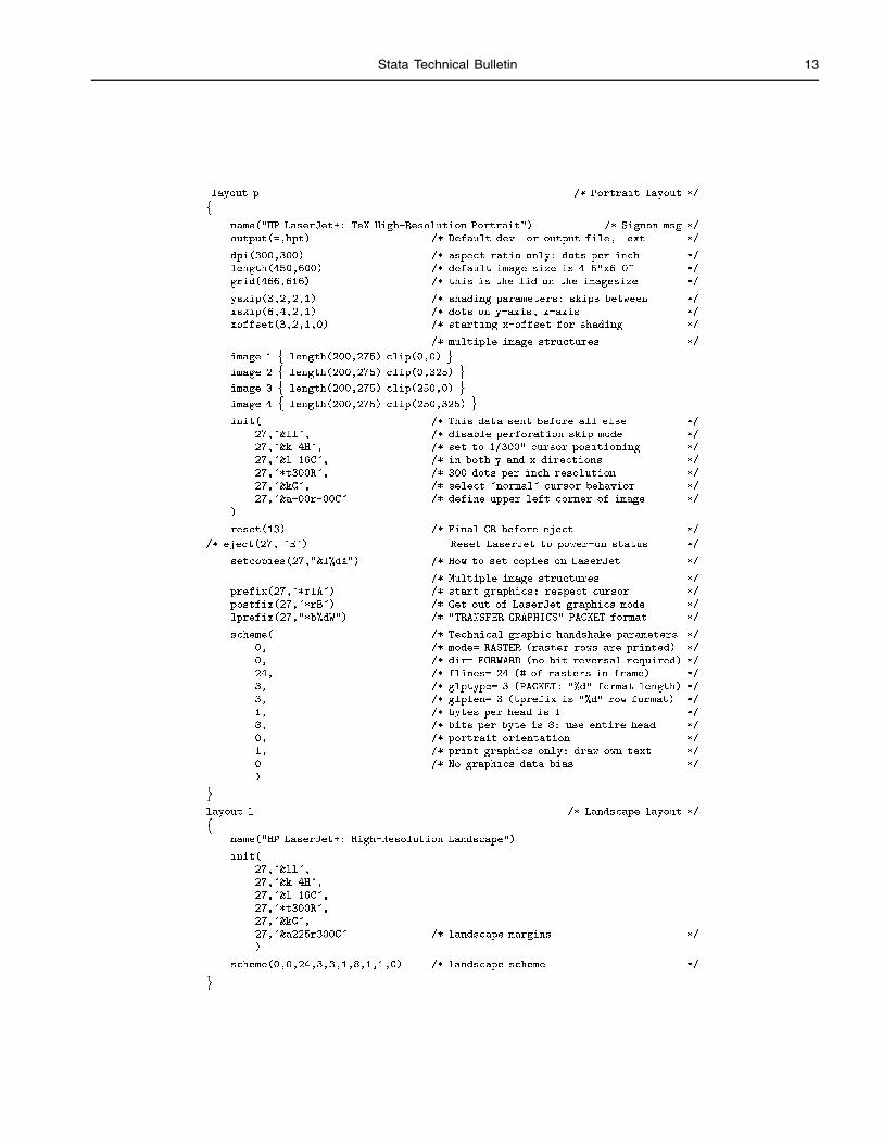
Stata Technical Bulletin 13
layout p /* Portrait layout */
f
name("HP LaserJet+: TeX High-Resolution Portrait") /* Signon msg */
output(=,hpt) /* Default dev. or output file, .ext */
dpi(300,300) /* aspect ratio only: dots per inch */
length(450,600) /* default image size is 4.5"x6.0" */
grid(466,616) /* this is the lid on the imagesize */
yskip(3,2,2,1) /* shading parameters: skips between */
xskip(6,4,2,1) /* dots on y-axis, x-axis */
xoffset(3,2,1,0) /* starting x-offset for shading */
/* multiple image structures */
image 1 f length(200,275) clip(0,0) gimage 2 f length(200,275) clip(0,325) gimage 3 f length(200,275) clip(250,0) gimage 4 f length(200,275) clip(250,325) g
init( /* This data sent before all else */
27,'&ll', /* disable perforation skip mode */
27,'&k.4H', /* set to 1/300" cursor positioning */
27,'&l.16C', /* in both y and x directions */
27,'*t300R', /* 300 dots per inch resolution */
27,'&kG', /* select 'normal' cursor behavior */
27,'&a-00r-00C' /* define upper left corner of image */
)
reset(13) /* Final CR before eject */
/* eject(27, 'E') Reset LaserJet to power-on status */
setcopies(27,"&l%dX") /* How to set copies on LaserJet */
/* Multiple image structures */
prefix(27,'*r1A') /* start graphics: respect cursor */
postfix(27,'*rB') /* Get out of LaserJet graphics mode */
lprefix(27,"*b%dW") /* "TRANSFER GRAPHICS" PACKET format */
scheme( /* Technical graphic handshake parameters */
0, /* mode= RASTER (raster rows are printed) */
0, /* dir= FORWARD (no bit reversal required) */
24, /* flines= 24 (# of rasters in frame) */
3, /* glptype= 3 (PACKET: "%d" format length) */
3, /* glplen= 3 (tprefix is "%d" row format) */
1, /* bytes per head is 1 */
8, /* bits per byte is 8: use entire head */
0, /* portrait orientation */
1, /* print graphics only: draw own text */
0 /* No graphics data bias */
)
g
layout l /* Landscape layout */
fname("HP LaserJet+: High-Resolution Landscape")
init(
27,'&ll',
27,'&k.4H',
27,'&l.16C',
27,'*t300R',
27,'&kG',
27,'&a225r300C' /* landscape margins */
)
scheme(0,0,24,3,3,1,8,1,1,0) /* landscape scheme */
g
14 Stata Technical Bulletin STB-19
Before I explain the modifications, let me give you an overview of this file. tex.dot is broken into two sections: layout p
which tells gphdot the specifications for a portrait layout, and layout l which makes a few modifications to these specificationsfor a landscape layout. Each line of the file is a gphdot command. For example, the command “dpi(300,300)” tells gphdot
to print the graph at a resolution of 300 dots per inch in both the horizontal and vertical directions. The comment to the rightof each command provides a pretty decent clue to the command’s purpose and syntax.
Only four lines were changed to make hplphr.dot into tex.dot. The sign-on message (the name()) command waschanged in an obvious and inessential way. The output() command, on the next line, was also changed. In hplphr.dot thisline reads (ignoring comments)
output(PRN:,hpl)
which indicates that the output of gphdot should be sent to PRN: by default or given a file extension of .hpl if the output issaved in a file. In tex.dot, that command is changed to
output(=,hpt)
which indicates that the output of gphdot is always to be saved in a file with the extension .hpt, a mnemonic for Hewlett-PackardTEX file.
The next change occurs in the init() command. This command sends a stream of characters to the printer to initialize it,that is, to place it in the appropriate state to receive the graph. The ubiquitous “27” is the ASCII code for the escape characterwhich the LaserJet expects to precede each initialization command. One line is changed. The line that, in hplphr.dot, used toread
27,'&a300r300C'
has been replaced by the line that reads:
27,'&a-00r-00C'
hplphr.dot assumes the graph is the only thing on the page, so it leaves a border at the top and left of the graph. tex.dotknows the graph will be stuck in a TEX document, so it eliminates the border and specifies that the graph should begin whereverthe cursor happens to be. This change wasn’t carried through in the landscape layout. The landscape layout is never used in theSTB, so we got a bit careless in changing that section of the code. If we ever start including landscape layout graphs, we wouldchange this line in that layout as well.
Finally, the line
eject(27, 'E')
is commented out. As the comment next to the command indicates, Stata normally resets the printer to its power-on status afterprinting a graph so the next print job begins with a clean slate. Resetting the printer in the middle of printing a TEX documentwould be disastrous, so we simply suppress that command.
ReferencesBecketti, S. gr13.1: \specialfg effects with Stata graphs in TEX documents. Stata Technical Bulletin 15: 12–13.
Soon, T. W. and S. L. C. Saw. gr13: Incorporating Stata-created PostScript files into TEX/LATEX documents. Stata Technical Bulletin 15: 7–12.
os12 Windowed interfaces for Stata
William Gould, Stata Corporation, FAX 409-696-4601
StataQuest [see an44 in this issue—Ed.] is a version of Stata intended for use in teaching undergraduate statistics and ismarketed by Duxbury Press. From Stata Corporation’s point of view, however, StataQuest represents an experiment, the resultof which will determine how windowed interfaces will work in future versions of Stata.
Although StataQuest is based on Stata 3.1, it has features that are lacking from the 3.1 product, the most important of whichis a pull-down menu interface. My comments on windowed interfaces are, by now, well known (Gould 1992, 1993a, 1993b), soit will surprise nobody that Stata’s command language survives intact. By the same token, I have previously admitted in printthat Stata needs a alternative windowed interface and I am now willing to admit that Stata has by now grown so large (broad?)that even those intimate with Stata (such as myself) forget exactly how some feature rarely used by me—frequently used byothers—works. It is here that windowed interfaces work well.
Stata Technical Bulletin 15
We are, at a technical level, rather proud of StataQuest’s menu system. We are proud because we made only two additions toStata’s underlying C code and thereafter implemented the entire top-line menu bar, pull-down window, pop-up warnings interfacein Stata’s ado language! This allowed us to implement the system on the Macintosh and under DOS using the same ado-files,thus ensuring compatibility.1 Moreover, this continues our open-system design that will allow others to implement programsusing menus.
This code-organization trick also allowed us to develop a menu system quickly and, in fact, we presented Duxbury with morethan one look and feel—the first was dramatically changed before becoming final (thanks to Ted Anagnoson’s, Rich DeLeon’s,and especially Stan Loll’s demanding comments). The implementation as ado-files allowed dramatic changes without rewritinglarge blocks of low-level code.
At a technical level, I feel confident declaring the menu system a success. End users, however, experience something otherthan the internal elegance with which the code carries forth their requests, and determination of whether the menu system reallyis a success will have to wait for end-user reports. It is this sense in which StataQuest is an experiment.
It is unlikely that results will prove fully positive or fully negative. In our own testing, we find things that we would dodifferently—will do differently—and we expect users will make comments that will similarly improve the design. Therefore, Iask that even if you have no interest in undergraduate teaching, you try StataQuest. If you subscribe to the STB with magneticmedia, the diskette is included. We are actively seeking comments.
One aspect of the menu design we already know will be successful is the full-screen, spreadsheet data editor. Expect to seethis component in the next release of Stata.
The menu system’s elegant internal design is due to Bill Rogers. The menu system’s rather obvious external look and feelis due to Ted Anagnoson, Richard DeLeon, Stan Loll, Alan Riley, Bill Rogers, and me, and thus blame, if any, is appropriatelyspread. The menu system’s compulsion to show the command you could have typed in command mode to achieve the sameresult is due to me.
Notes
1. That is actually not quite true, but it will be true next time around. This time, we did the DOS version first and, withour knowledge of the Macintosh, tried to ensure that our command set was rich enough. Of course, when we got to theMacintosh, we found it was not and had to introduce some changes. Deadlines were such that we could not iterate onemore time and so bring the two versions into full agreement, but we are now performing that iteration for our own futureuse.
ReferencesGould, W. 1992. os7: Stata and windowed operating systems. Stata Technical Bulletin 10: 18–20.
——. 1993a. os7.2: Stata and windowed operating systems: Response to comment by W. Rising. Stata Technical Bulletin 11: 10.
——. 1993b. os7.3: CRC committed to Stata’s command language. Stata Technical Bulletin 11: 10.
os13 Using awk and fgrep for selective extraction from Stata log files
Nicholas J. Cox, Department of Geography, University of Durham, UKFAX (011)-44-91-374 2456, EMAIL [email protected]
In STB-14, Rising (1993) introduced two ado-files, addnote and notefile, for taking notes during a Stata session. Anotherapproach to the problem is to keep a log file, using the log command, and to make comments using * as the first charactertyped on the command line. After a Stata session, it is easy to extract such lines from the log file using awk, a standard featureof Unix systems that is also readily available for machines running DOS. The more general problem is selective extraction froma log file of particular kinds of material. A further example involves the output from inspect, which may be selected by usingfgrep.
Comments in log files
You are running Stata and you open a log file by typing
. log using filename
16 Stata Technical Bulletin STB-19
(see [4] logs in the manual if not familiar with the idea). You can comment on the results for later reference by starting whatyou type on any command line with *; for example,
. * outlier for annual rainfall about 12000 mm on the scatter plot
. * needs checking: probably an error
(see [2] comments in the manual).
After leaving Stata, these comments can be extracted from the log file filename.log. My approach is to use a one-line awk
program
awk '$2 ~/*/' filename.log > comments.txt
which routes all lines whose second fields (“$2”) contain * to a new file called comments.txt. The first field of comment linesis always the period prompt (.) that Stata copies to log files, followed by a space. By default, awk defines a field as a set ofcharacters on a line separated from other fields by white space. The pattern specified above includes not only lines like
. * space following asterisk
but also lines like
. *no space following asterisk
awk is a programming language that is especially useful for file processing. awk is a standard part of Unix systems. Thedefinitive book on awk, which is excellent, is Aho, Kernighan and Weinberger (1988). awk is not restricted to those workingunder Unix. Those who (like me) work mostly with DOS machines can use a public domain version such as GNU awk or acommercial version such as the one from Mortice Kern Systems.
Selective extraction in general
The more general problem can be identified as that of selective extraction from a log file. Even a short and simple Statasession may lead to a log file that is hundreds or thousands of lines long, much of which may have no permanent value. Manyusers edit a log file interactively soon after a session to eliminate dead ends, outright mistakes, and useless material. Sometimesa more systematic approach is in order.
One common task is checking a data file. Data sets with many categorical variables need extensive labeling, and I oftenfind that there are data values not documented in the value labels. In such circumstances, the useful command inspect (see[5d] inspect in the manual) produces a message ending
NOT documented in the label.
I have a standard do-file check.do which is simply
set more 1
inspect _all
So I would do something like this:
log using check
do check
log close
!fgrep NOT check.log
Having set more 1, what may be tens or hundreds of screenfuls of output from inspect scroll by rapidly, but the lines required,which contain NOT, are found by fgrep. The prefix ! informs Stata that what follows is not a Stata command. Each deficientvariable may then be checked in detail. Again, fgrep (or fast grep) is a standard part of Unix that can be obtained for DOS
machines from public domain libraries or commercially available sets of Unix-like utilities. Alternatively, something very similarmay be done with the DOS command find. You could also use awk.
Admittedly, fgrep may find something irrelevant, say if you have a variable called NOT, but in my experience that has notbeen a real problem. Similarly, in the first problem, does Stata ever put * as part of the second field of an output line? If itdoes, the more restrictive pattern in
awk '$1 == "." && $2 ~/*/' filename.log > comments.txt
Stata Technical Bulletin 17
may be used instead, specifying that the first field must be a period and the second field must contain *.
Other kinds of selective extraction often yield to an ad hoc approach. You can write a short awk program exploiting thefact that the stuff you want is on lines with seven fields, or whatever.
Incidentally, awk is also very useful for checking data files. Short programs, often one line in length, can be written tocheck that all lines have the same number of fields, that there are no blank lines, that all data are numeric, and so forth.
ReferencesAho, A. V., B. W. Kernighan, and P. J. Weinberger. 1988. The Awk Programming Language. Reading, MA: Addison–Wesley.
Rising, B. 1993. os10: A method for taking notes during a Stata session. Stata Technical Bulletin 14: 10–11.
sg22.3 Generalized linear models: revision of glm. Rejoinder
Patrick Royston, Royal Postgraduate Medical School, London, FAX (011)-44-81-740-3119
In response to factual issues raised by Hilbe’s (1994) comments on Royston (1994):
1. The �2-distribution-based p-values for the deviance and Pearson �
2 statistics are inaccurate for both the binomial andthe Poisson distributions. Quoting McCullagh and Nelder (1989, p. 119): “The deviance function [for models for binarydata] is most directly useful not as an absolute measure of goodness-of-fit but for comparing two nested models : : : Inparticular, D(Y ; �0) need not have an approximate �
2 distribution nor need it be distributed independently of �0. The�2 approximation is usually quite accurate for differences of deviances even though it is inaccurate for the deviances
themselves.” This comment is underlined on page 122: “It is good statistical practice, however, not to rely on either D orX
2 [the Pearson �2] as an absolute measure of goodness of fit in these circumstances.” From the same source (p. 197):
“Another approximation to [the Poisson deviance] D(Y ;�) for large � is obtained by expanding [it] as a Taylor series in(y � �)=�. We find
D(Y ;�) 'Xi
(yi� �
i)2=�
i
which is less accurate than the quadratic on the �1=3 scale. This statistic is due to Pearson (1900).” With the possible
exception of the negative binomial (the distribution of whose deviance McCullagh and Nelder do not discuss), the p-valuesfor the discrete distributions fitted by glm and glmr are accurate only in large samples, so it seems potentially misleadingfor the software to display them.
2. glmr supports all the power links provided by glm and adds a new link, link(opower), which generalizes the logit linkfor the binomial distribution. Specifically, the formula for this link function is
g(�) =���(m� �)
��
where � is the mean of Y (given the covariates) and m is the binomial denominator. The identity (� = 1) flavor of this linkmay be useful in epidemiology to model risk effects expressed as odds on an additive scale, rather than on the multiplicativescale provided by the ubiquitous logit link. Thus glmr actually provides more models than glm rather than fewer.
ReferencesHilbe, J. 1994. sg22.1: Comment on Royston’s revision of glm. Stata Technical Bulletin 18: 11–13.
Royston, P. 1994. sg22: Generalized linear models: revision of glm. Stata Technical Bulletin 18: 6–11.
McCullagh, P. and J. A. Nelder. 1989. Generalized Linear Models, 2d ed. London: Chapman and Hall.
sqv9 Probit coefficients as changes in probabilities
William Gould, Stata Corporation, FAX 409-696-4601
The syntax of dprobit is
dprobit depvar indepvars�weight
� �if exp
� �in range
� �, at(fxbarjpbarj#g) classic probit options
�aweights and fweights are allowed.
dprobit shares the features of all estimation commands; see [4] estimate.
To reset problem-size limits, see [5u] matsize.
18 Stata Technical Bulletin STB-19
Description
dprobit estimates maximum-likelihood probit models and is an alternative to probit; see [5s] logit. Rather than reportingthe coefficients, however, dprobit reports the change in the probability for an infinitesimal change in each independent,continuous variable and, by default, the discrete change in the probability for dummy variables. smallskip
dprobit typed without arguments redisplays results. probit may also be typed without arguments after dprobit estimationto see the model in coefficient form.
Options
at(fxbarjpbarj#g) specifies the point around which the transformation of results is to be made. at(xbar) is the default,meaning the transformation is made at the predicted probability of a positive outcome evaluated at the means of theindependent variables: ~p = XB. at(pbar) specifies the transformation is made at the observed overall fraction of positiveoutcomes: ~p = �p. at(#) allows the transformation to be made around any user specified point ~p = #, 0 < # < 1. at()may be specified when the model is estimated or when results are redisplayed.
smallskip classic requests that the mean effects be calculated using the formula f(~p)bi
in all cases. If classic
is not specified, f(~p)bi
is used for continuous variables but the mean effects for dummy variables is calculated asF (~p � b
i�xi+ b
i) � F (~p � b
i�xi). classic may be specified at estimation time or when results are redisplayed. Results
calculated without classic may be redisplayed with classic and vice versa.
smallskip probit options refers to any of the options of the probit command.
Remarks
A probit model is defined
P(yj6= 0) = F (XB)
where F () is the cumulative normal with mean 0 and variance 1. XB is the called the probit score or index. If, for someobservation, XB is 0, then the corresponding probability is the area under the normal density between �1 and 0, written F (0),or .5. If XB is 1, then the probability is the area between 1 and 1, F (1) or, in Stata, normprob(1), which is .8413. If XB is�1, the probability is the area between 1 and �1, F (�1), or .1587.
XB has a normal distribution and variables with normal distributions are often written using the letter z. Interpreting probitcoefficients requires thinking in the z metric. For instance, pretend we estimated the probit equation:
P(yj6= 0) = F (:08233� x1 + 1:529� x2 � 3:139)
The interpretation of the x2 coefficient is that each one-unit increase in x2 leads to increasing the probit index by 1.529 standarddeviations. 1.529 standard deviations should strike you as a lot. For instance, at the center of the normal distribution F (0) = .5,increasing the index by 1.529 would lead to F (1.529) = .9369. If you started far in the left tail, say at �2, F (�2) = .0228and F (�2 + 1.529) = .3188. If you started far in the right tail, say at 2, F (2) = .9772 and F (2 + 1.529) = .9998.
How much a one-unit change in x2 affects the probability of a positive outcome depends on where you start, but the rightway to think about it is that you are shifting out 1.529 standard deviation units along the normal no matter where you start andthat is a long ways.
Learning to think in the z metric takes practice and, even if you do, communicating results to others who have not learnedto think this way is difficult. One quickly finds oneself resorting to statements like “it’s a lot—a whole lot—not a stupefyingamount, but big.” This is less than satisfactory.
A transformation of the results helps many people think about them. The change in the probability somehow feels morenatural, but how big that change is depends on where we start. Why not choose as a starting point the mean of the data? Thus,rather than reporting 1.529, if the mean probability of success in the data were 21=69 = .3043, we would report something like.5411, meaning the change in the probability evaluated at the mean. We could make the calculation as follows:
Stata Technical Bulletin 19
At the mean probability of success in the data of .3043, the normal index is F�1(.3043) = �.5121. Adding our coefficientof 1.529 to this result and recalculating the probability, we get F (�.5121+ 1.529) = .8454. Thus, the change in the probabilityis .8454� .3043 = .5411.
In practice, people who use probit make this calculation somewhat differently and produce a slightly different number.Rather than make the calculation for a one-unit change in x, they calculate the slope of the probability function. Doing a littlecalculus, they derive that the change in the probability for a change in x2 (@F=@x2) is the height of the normal density at themean score corresponding to probability of success, multiplied by the x2 coefficient. Going through this calculation, they wouldget .5351.
The difference between .5411 and .5351 is not much; they differ because the .5411 is the exact answer for a one-unit changein x2 whereas .5351 is the answer for an infinitesimal change extrapolated out.
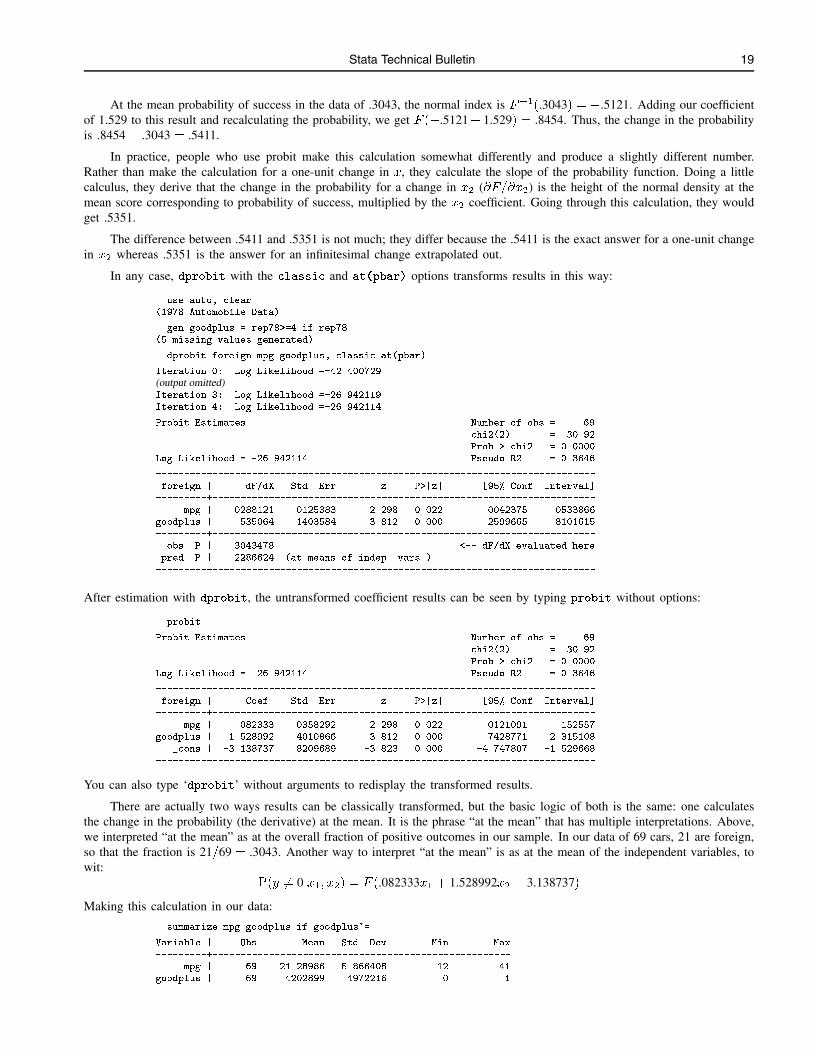
In any case, dprobit with the classic and at(pbar) options transforms results in this way:
. use auto, clear
(1978 Automobile Data)
. gen goodplus = rep78>=4 if rep78�.
(5 missing values generated)
. dprobit foreign mpg goodplus, classic at(pbar)
Iteration 0: Log Likelihood =-42.400729
(output omitted)Iteration 3: Log Likelihood =-26.942119
Iteration 4: Log Likelihood =-26.942114
Probit Estimates Number of obs = 69
chi2(2) = 30.92
Prob > chi2 = 0.0000
Log Likelihood = -26.942114 Pseudo R2 = 0.3646
------------------------------------------------------------------------------
foreign | dF/dX Std. Err. z P>|z| [95% Conf. Interval]
---------+--------------------------------------------------------------------
mpg | .0288121 .0125383 2.298 0.022 .0042375 .0533866
goodplus | .535064 .1403584 3.812 0.000 .2599665 .8101615
---------+--------------------------------------------------------------------
obs. P | .3043478 <-- dF/dX evaluated here
pred. P | .2286624 (at means of indep. vars.)
------------------------------------------------------------------------------
After estimation with dprobit, the untransformed coefficient results can be seen by typing probit without options:
. probit
Probit Estimates Number of obs = 69
chi2(2) = 30.92
Prob > chi2 = 0.0000
Log Likelihood = -26.942114 Pseudo R2 = 0.3646
------------------------------------------------------------------------------
foreign | Coef. Std. Err. z P>|z| [95% Conf. Interval]
---------+--------------------------------------------------------------------
mpg | .082333 .0358292 2.298 0.022 .0121091 .152557
goodplus | 1.528992 .4010866 3.812 0.000 .7428771 2.315108
_cons | -3.138737 .8209689 -3.823 0.000 -4.747807 -1.529668
------------------------------------------------------------------------------
You can also type ‘dprobit’ without arguments to redisplay the transformed results.
There are actually two ways results can be classically transformed, but the basic logic of both is the same: one calculatesthe change in the probability (the derivative) at the mean. It is the phrase “at the mean” that has multiple interpretations. Above,we interpreted “at the mean” as at the overall fraction of positive outcomes in our sample. In our data of 69 cars, 21 are foreign,so that the fraction is 21=69 = .3043. Another way to interpret “at the mean” is as at the mean of the independent variables, towit:
P(y 6= 0j�x1; �x2) = F (.082333�x1 + 1.528992�x2 � 3.138737)
Making this calculation in our data:
. summarize mpg goodplus if goodplus~=.
Variable | Obs Mean Std. Dev. Min Max
---------+-----------------------------------------------------
mpg | 69 21.28986 5.866408 12 41
goodplus | 69 .4202899 .4972216 0 1
20 Stata Technical Bulletin STB-19
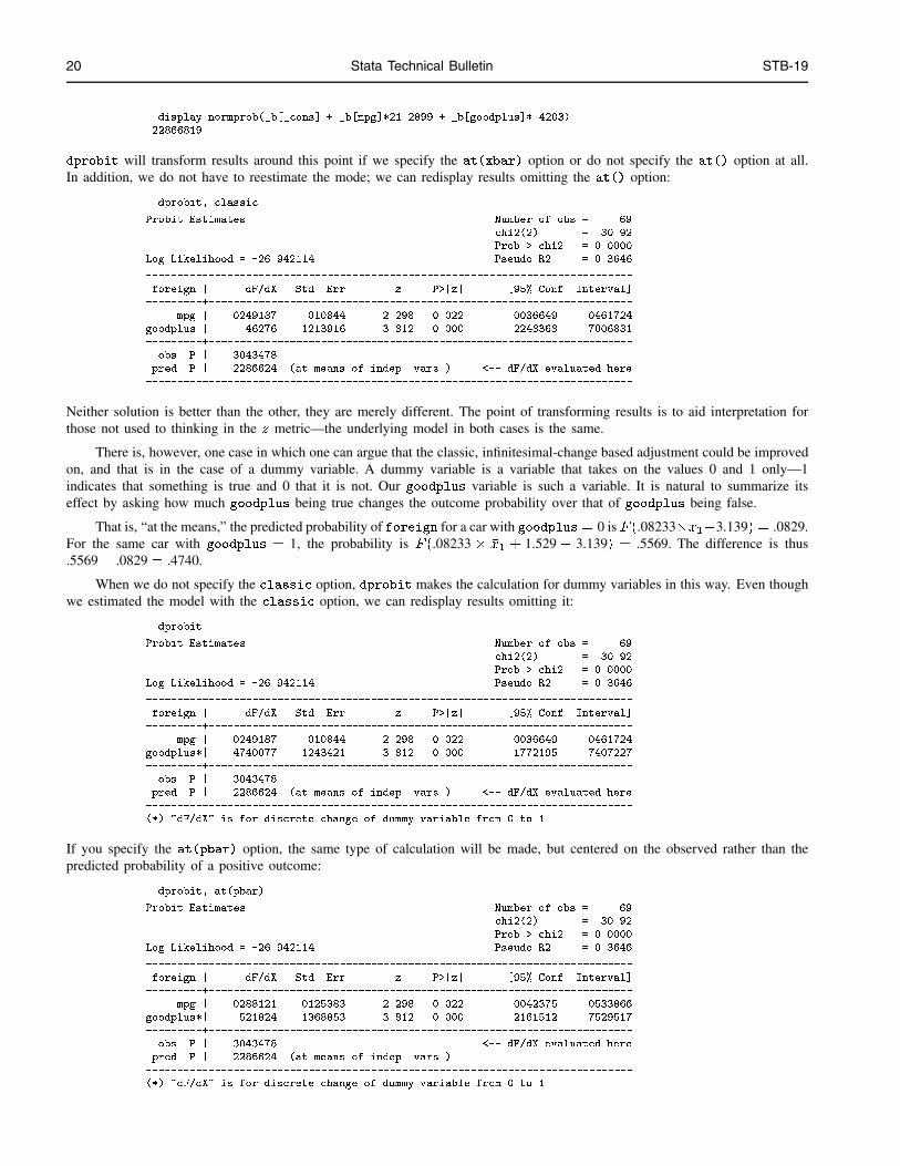
. display normprob(_b[_cons] + _b[mpg]*21.2899 + _b[goodplus]*.4203)
.22866819
dprobit will transform results around this point if we specify the at(xbar) option or do not specify the at() option at all.In addition, we do not have to reestimate the mode; we can redisplay results omitting the at() option:
. dprobit, classic
Probit Estimates Number of obs = 69
chi2(2) = 30.92
Prob > chi2 = 0.0000
Log Likelihood = -26.942114 Pseudo R2 = 0.3646
------------------------------------------------------------------------------
foreign | dF/dX Std. Err. z P>|z| [95% Conf. Interval]
---------+--------------------------------------------------------------------
mpg | .0249187 .010844 2.298 0.022 .0036649 .0461724
goodplus | .46276 .1213916 3.812 0.000 .2248368 .7006831
---------+--------------------------------------------------------------------
obs. P | .3043478
pred. P | .2286624 (at means of indep. vars.) <-- dF/dX evaluated here
------------------------------------------------------------------------------
Neither solution is better than the other, they are merely different. The point of transforming results is to aid interpretation forthose not used to thinking in the z metric—the underlying model in both cases is the same.
There is, however, one case in which one can argue that the classic, infinitesimal-change based adjustment could be improvedon, and that is in the case of a dummy variable. A dummy variable is a variable that takes on the values 0 and 1 only—1indicates that something is true and 0 that it is not. Our goodplus variable is such a variable. It is natural to summarize itseffect by asking how much goodplus being true changes the outcome probability over that of goodplus being false.
That is, “at the means,” the predicted probability of foreign for a car with goodplus = 0 is F (.08233��x1�3.139) = .0829.For the same car with goodplus = 1, the probability is F (.08233 � �x1 + 1.529 � 3.139) = .5569. The difference is thus.5569� .0829 = .4740.
When we do not specify the classic option, dprobit makes the calculation for dummy variables in this way. Even thoughwe estimated the model with the classic option, we can redisplay results omitting it:
. dprobit
Probit Estimates Number of obs = 69
chi2(2) = 30.92
Prob > chi2 = 0.0000
Log Likelihood = -26.942114 Pseudo R2 = 0.3646
------------------------------------------------------------------------------
foreign | dF/dX Std. Err. z P>|z| [95% Conf. Interval]
---------+--------------------------------------------------------------------
mpg | .0249187 .010844 2.298 0.022 .0036649 .0461724
goodplus*| .4740077 .1243421 3.812 0.000 .1772195 .7407227
---------+--------------------------------------------------------------------
obs. P | .3043478
pred. P | .2286624 (at means of indep. vars.) <-- dF/dX evaluated here
------------------------------------------------------------------------------
(*) "dF/dX" is for discrete change of dummy variable from 0 to 1
If you specify the at(pbar) option, the same type of calculation will be made, but centered on the observed rather than thepredicted probability of a positive outcome:
. dprobit, at(pbar)
Probit Estimates Number of obs = 69
chi2(2) = 30.92
Prob > chi2 = 0.0000
Log Likelihood = -26.942114 Pseudo R2 = 0.3646
------------------------------------------------------------------------------
foreign | dF/dX Std. Err. z P>|z| [95% Conf. Interval]
---------+--------------------------------------------------------------------
mpg | .0288121 .0125383 2.298 0.022 .0042375 .0533866
goodplus*| .521824 .1368853 3.812 0.000 .2161512 .7529517
---------+--------------------------------------------------------------------
obs. P | .3043478 <-- dF/dX evaluated here
pred. P | .2286624 (at means of indep. vars.)
------------------------------------------------------------------------------
(*) "dF/dX" is for discrete change of dummy variable from 0 to 1
Stata Technical Bulletin 21
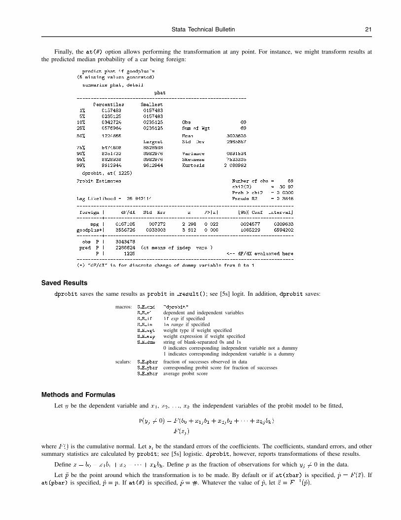
Finally, the at(#) option allows performing the transformation at any point. For instance, we might transform results atthe predicted median probability of a car being foreign:
. predict phat if goodplus~=.
(5 missing values generated)
. summarize phat, detail
phat
-------------------------------------------------------------
Percentiles Smallest
1% .0157483 .0157483
5% .0235125 .0157483
10% .0342724 .0235125 Obs 69
25% .0576964 .0235125 Sum of Wgt. 69
50% .1224665 Mean .3003605
Largest Std. Dev. .2985857
75% .5474608 .8828938
90% .8051732 .8982976 Variance .0891534
95% .8828938 .8982976 Skewness .7533305
99% .9612944 .9612944 Kurtosis 2.088962
. dprobit, at(.1225)
Probit Estimates Number of obs = 69
chi2(2) = 30.92
Prob > chi2 = 0.0000
Log Likelihood = -26.942114 Pseudo R2 = 0.3646
------------------------------------------------------------------------------
foreign | dF/dX Std. Err. z P>|z| [95% Conf. Interval]
---------+--------------------------------------------------------------------
mpg | .0167105 .007272 2.298 0.022 .0024577 .0309633
goodplus*| .3556726 .0933003 3.812 0.000 .1085229 .6594202
---------+--------------------------------------------------------------------
obs. P | .3043478
pred. P | .2286624 (at means of indep. vars.)
P | .1225 <-- dF/dX evaluated here
------------------------------------------------------------------------------
(*) "dF/dX" is for discrete change of dummy variable from 0 to 1
Saved Results
dprobit saves the same results as probit in result(); see [5s] logit. In addition, dprobit saves:
macros: S E cmd "dprobit"
S E vl dependent and independent variablesS E if if exp if specifiedS E in in range if specifiedS E wgt weight type if weight specifiedS E exp weight expression if weight specifiedS E dum string of blank-separated 0s and 1s
0 indicates corresponding independent variable not a dummy1 indicates corresponding independent variable is a dummy
scalars: S E pbar fraction of successes observed in dataS E ybar corresponding probit score for fraction of successesS E xbar average probit score
Methods and Formulas
Let y be the dependent variable and x1, x2, : : :, xk
the independent variables of the probit model to be fitted,
P(yj6= 0) = F (b0 + x1jb1 + x2jb2 + � � �+ x
kjbk)
= F (zj)
where F () is the cumulative normal. Let si
be the standard errors of the coefficients. The coefficients, standard errors, and othersummary statistics are calculated by probit; see [5s] logistic. dprobit, however, reports transformations of these results.
Define �z = b0 + �x1b1 + �x2 + � � �+ �xkbk
. Define �p as the fraction of observations for which yj6= 0 in the data.
Let ~p be the point around which the transformation is to be made. By default or if at(xbar) is specified, ~p = F (�z). Ifat(pbar) is specified, ~p = �p. If at(#) is specified, ~p = #. Whatever the value of ~p, let ~z = F
�1(~p).
22 Stata Technical Bulletin STB-19
For continuous variables, or for all variables if classic is specified, dprobit reports
b�
i=
@F (z)
@xi
����z=~z
= f(~z)bi
where f() is the normal density. The reported standard error for this quantity is s�i= f(~z)s
i, and thus the reported z statistic is
b�
i=s
�
i= f(~z)b
i=(f(~z)s
i) = b
i=s
iand so is identical to the test for the coefficient being zero reported by probit. The upper
and lower confidence intervals are calculated as b�i� z
�s�
i.
For dummy variables taking on the values 0 and 1 when classic is not specified, dprobit makes the discrete calculationassociated with the dummy changing from 0 to 1. Define
zi0 = ~z � �x
ibi
which is the “mean” value of the score associated with xi= 0. dprobit reports:
b�
i= F (z
i0 + bi)� F (z
i0)
The standard error of this quantity is calculated as s�i= b
�
isi=b
i, so once again b�
i=s
�
i= b
i=s
iand the test of the difference being
zero corresponds to that for the coefficient bi
being zero. The lower and upper limits for the confidence interval are calculatedas F (z
i0 + bi� z
�si)� F (z
i0).
ssa3 Adjusted survival curves
William H. Rogers, Stata Corporation, FAX 409-696-4601
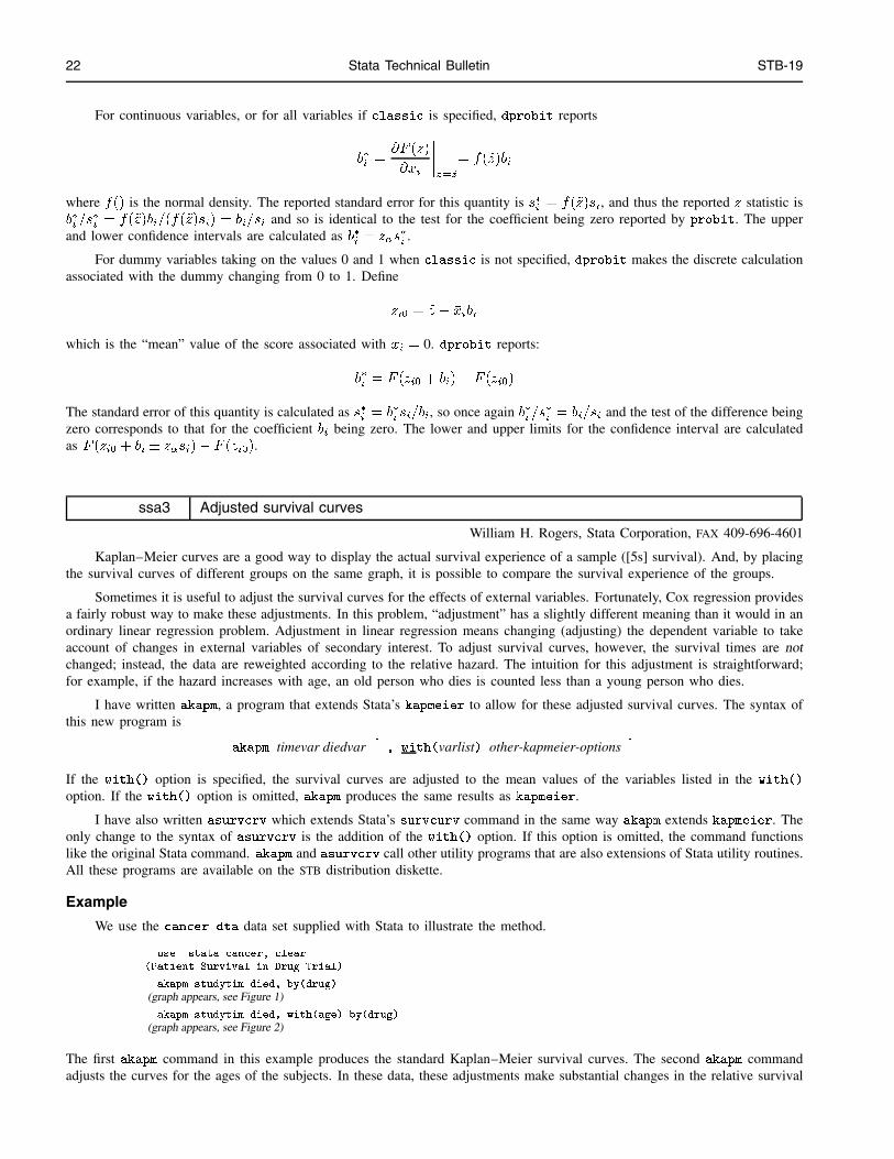
Kaplan–Meier curves are a good way to display the actual survival experience of a sample ([5s] survival). And, by placingthe survival curves of different groups on the same graph, it is possible to compare the survival experience of the groups.
Sometimes it is useful to adjust the survival curves for the effects of external variables. Fortunately, Cox regression providesa fairly robust way to make these adjustments. In this problem, “adjustment” has a slightly different meaning than it would in anordinary linear regression problem. Adjustment in linear regression means changing (adjusting) the dependent variable to takeaccount of changes in external variables of secondary interest. To adjust survival curves, however, the survival times are notchanged; instead, the data are reweighted according to the relative hazard. The intuition for this adjustment is straightforward;for example, if the hazard increases with age, an old person who dies is counted less than a young person who dies.
I have written akapm, a program that extends Stata’s kapmeier to allow for these adjusted survival curves. The syntax ofthis new program is
akapm timevar diedvar�, with(varlist) other-kapmeier-options
�If the with() option is specified, the survival curves are adjusted to the mean values of the variables listed in the with()
option. If the with() option is omitted, akapm produces the same results as kapmeier.
I have also written asurvcrv which extends Stata’s survcurv command in the same way akapm extends kapmeier. Theonly change to the syntax of asurvcrv is the addition of the with() option. If this option is omitted, the command functionslike the original Stata command. akapm and asurvcrv call other utility programs that are also extensions of Stata utility routines.All these programs are available on the STB distribution diskette.
Example
We use the cancer.dta data set supplied with Stata to illustrate the method.
. use \stata\cancer, clear
(Patient Survival in Drug Trial)
. akapm studytim died, by(drug)
(graph appears, see Figure 1)
. akapm studytim died, with(age) by(drug)
(graph appears, see Figure 2)
The first akapm command in this example produces the standard Kaplan–Meier survival curves. The second akapm commandadjusts the curves for the ages of the subjects. In these data, these adjustments make substantial changes in the relative survival
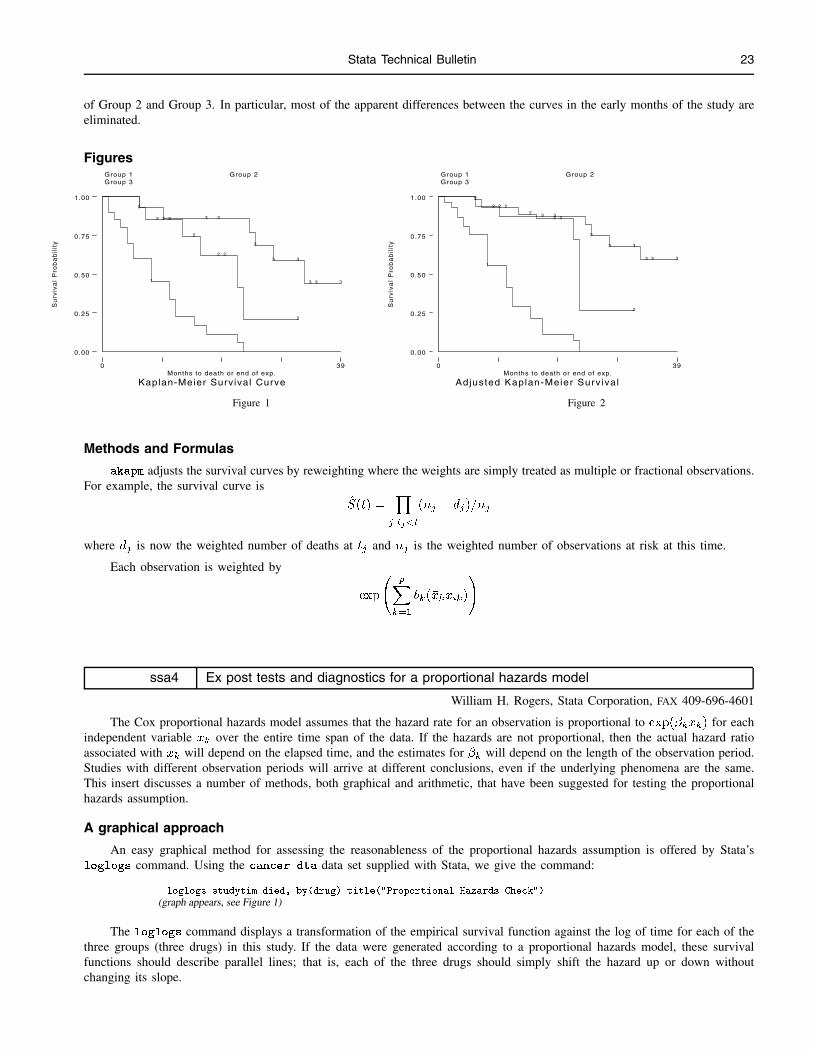
Stata Technical Bulletin 23
of Group 2 and Group 3. In particular, most of the apparent differences between the curves in the early months of the study areeliminated.
Figures
Su
rviv
al
Pro
ba
bil
ity
Kaplan-Meier Survival CurveMonths to death or end of exp.
Group 1 Group 2 Group 3
0 39
0.00
0.25
0.50
0.75
1.00
1
2
2 2 2
2
2 2
2
3 3
3
3 3
3 3 3
Su
rviv
al
Pro
ba
bil
ity
Ad justed Kaplan-Meier SurvivalMonths to death or end of exp.
Group 1 Group 2 Group 3
0 39
0.00
0.25
0.50
0.75
1.00
1
2
2 2 2
22 2
2
3 3
3
3 3
3 3 3
Figure 1 Figure 2
Methods and Formulas
akapm adjusts the survival curves by reweighting where the weights are simply treated as multiple or fractional observations.For example, the survival curve is
S(t) =Y
jjtj<t
(nj� d
j)=n
j
where dj
is now the weighted number of deaths at tj
and nj
is the weighted number of observations at risk at this time.
Each observation is weighted by
exp
pX
k=1
bk(�x
kxik)
!
ssa4 Ex post tests and diagnostics for a proportional hazards model
William H. Rogers, Stata Corporation, FAX 409-696-4601
The Cox proportional hazards model assumes that the hazard rate for an observation is proportional to exp(�kxk) for each
independent variable xk
over the entire time span of the data. If the hazards are not proportional, then the actual hazard ratioassociated with x
kwill depend on the elapsed time, and the estimates for �
kwill depend on the length of the observation period.
Studies with different observation periods will arrive at different conclusions, even if the underlying phenomena are the same.This insert discusses a number of methods, both graphical and arithmetic, that have been suggested for testing the proportionalhazards assumption.
A graphical approach
An easy graphical method for assessing the reasonableness of the proportional hazards assumption is offered by Stata’sloglogs command. Using the cancer.dta data set supplied with Stata, we give the command:
. loglogs studytim died, by(drug) title("Proportional Hazards Check")
(graph appears, see Figure 1)
The loglogs command displays a transformation of the empirical survival function against the log of time for each of thethree groups (three drugs) in this study. If the data were generated according to a proportional hazards model, these survivalfunctions should describe parallel lines; that is, each of the three drugs should simply shift the hazard up or down withoutchanging its slope.
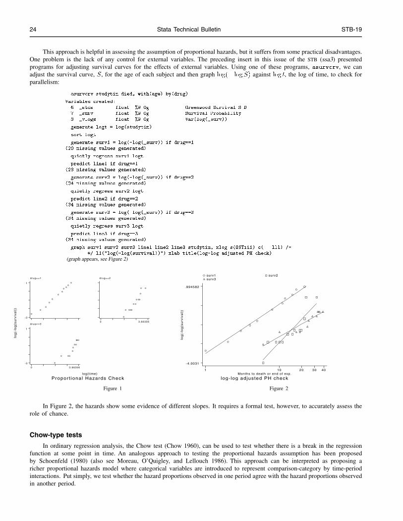
24 Stata Technical Bulletin STB-19
This approach is helpful in assessing the assumption of proportional hazards, but it suffers from some practical disadvantages.One problem is the lack of any control for external variables. The preceding insert in this issue of the STB (ssa3) presentedprograms for adjusting survival curves for the effects of external variables. Using one of these programs, asurvcrv, we canadjust the survival curve, S, for the age of each subject and then graph log(� logS) against log t, the log of time, to check forparallelism:
. asurvcrv studytim died, with(age) by(drug)
Variables created:
6. _stds float %9.0g Greenwood Survival S.D.
7. _surv float %9.0g Survival Probability
8. _vlogs float %9.0g Var(log(_surv))
. generate logt = log(studytim)
. sort logt
. generate surv1 = log(-log(_surv)) if drug==1
(29 missing values generated)
. quietly regress surv1 logt
. predict line1 if drug==1
(28 missing values generated)
. generate surv2 = log(-log(_surv)) if drug==2
(34 missing values generated)
. quietly regress surv2 logt
. predict line2 if drug==2
(34 missing values generated)
. generate surv3 = log(-log(_surv)) if drug==3
(34 missing values generated)
. quietly regress surv3 logt
. predict line3 if drug==3
(34 missing values generated)
. graph surv1 surv2 surv3 line1 line2 line3 studytim, xlog s(OSTiii) c(...lll) /*
*/ l1("log(-log(survival))") xlab title(log-log adjusted PH check)
(graph appears, see Figure 2)
log
(-lo
g(s
urv
iva
l))
P roport ional Hazards Checklog(time)
drug==1
-3
1
drug==2
0 3.66356drug==3
0 3.66356
-3
1
log
(-lo
g(s
urv
iva
l))
l og- log adjusted PH checkMonths to death or end of exp.
surv1 surv2 surv3
1 10 20 30 40
-4.0031
.994582
Figure 1 Figure 2
In Figure 2, the hazards show some evidence of different slopes. It requires a formal test, however, to accurately assess therole of chance.
Chow-type tests
In ordinary regression analysis, the Chow test (Chow 1960), can be used to test whether there is a break in the regressionfunction at some point in time. An analogous approach to testing the proportional hazards assumption has been proposedby Schoenfeld (1980) (also see Moreau, O’Quigley, and Lellouch 1986). This approach can be interpreted as proposing aricher proportional hazards model where categorical variables are introduced to represent comparison-category by time-periodinteractions. Put simply, we test whether the hazard proportions observed in one period agree with the hazard proportions observedin another period.
Stata Technical Bulletin 25
This approach, of course, leaves open the question of how to select the intervals. As with the Chow test, little guidance isavailable; indeed, the mathematics is presented as if different time periods could be specified for different categories.
I have written two programs that build on the approach of Schoenfeld. The two programs allow two different strategies forselecting intervals. In phtest1 (proportional hazards test 1), the first program, the user can either specify a single breakpoint inthe sample or leave it to the program to choose a breakpoint. phtest2, the second program, allows multiple breakpoints, butthe user must specify the location of all the breakpoints.
The syntax of phtest1 is
phtest1 timevar varlist�if exp
� �in range
� �,
f at(time) j divide(fraction) g dead(deadvar) iact(varlist2)�
The breakpoint is specified in one of three ways: with the at() option (e.g., type ‘at(15)’ to break the sample just prior tot = 15); with the divide() option (e.g., type ‘divide(.33)’ to break the sample so 1/3 of the deaths are before the breakpoint);or by specifying neither option (equivalent to typing ‘divide(.5)’). The iact() option specifies the variables whose effectswill be allowed to vary across the subsamples; if iact is omitted, all effects are held constant across subsamples. And, as inother survival analysis commands, the dead() option specifies the variable that indicates deaths.
The syntax of phtest2 is similar:
phtest2 timevar varlist�if exp
� �in range
�, at(time)
�dead(deadvar) iact(varlist2)
�In phtest2, the at() option is required and takes as arguments one or more time values.
In both commands, a richer time-varying Cox model is fit—according to the breakpoints and interactions specified—and alikelihood ratio test is used to detect a significant difference across breakpoints. Schoenfeld’s original method calculated observedand expected quantities in a set of cells and used a �
2 test to find differences. Moreau, et al. determined that one can use theWald variance estimator in this setting. We take this one step further and use the likelihood ratio test, because likelihood ratiotests tend to be more robust than Wald tests.
The interactions introduced are literally
interaction variable� I fobservation in early time frameg
Employing these methods in the present example, we find:
. tabulate drug, gen(d)
Drug type|
(1=placebo)| Freq. Percent Cum.
------------+-----------------------------------
1 | 20 41.67 41.67
2 | 14 29.17 70.83
3 | 14 29.17 100.00
------------+-----------------------------------
Total | 48 100.00
. phtest1 studytim age d2 d3, dead(died) iact(d2 d3)
Proportional hazards test with division just prior to t = 10
Chi-square(2) = 3.29, P = 0.1934
. phtest1 studytim age d3 if drug>=2, dead(died) iact(d3)
Proportional hazards test with division just prior to t = 16
Chi-square(1) = 1.03, P = 0.3104
. phtest2 studytim age d2 d3, dead(died) iact(age d2 d3) at(10 16)
Chi-square(6) = 4.33, P = 0.6320
In other words, the violations of proportional hazards that seem to be observed in Figure 2 cannot be confirmed and may wellbe due to chance.
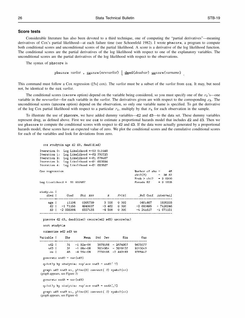
26 Stata Technical Bulletin STB-19
Score tests
Considerable literature has also been devoted to a third technique, one of computing the “partial derivatives”—meaningderivatives of Cox’s partial likelihood—at each failure time (see Schoenfeld 1982). I wrote phscore, a program to computeboth conditional scores and unconditional scores of the partial likelihood. A score is a derivative of the log likelihood function.The conditional scores are the partial derivatives of the log likelihood with respect to one of the explanatory variables. Theunconditional scores are the partial derivatives of the log likelihood with respect to the observations.
The syntax of phscore is
phscore varlist , cscore(newvarlist)�dead(deadvar) uscore(varname)
�This command must follow a Cox regression ([5s] cox). The varlist must be a subset of the varlist from cox. It may, but neednot, be identical to the cox varlist.
The conditional scores (cscore option) depend on the variable being considered, so you must specify one of the xk
’s—onevariable in the newvarlist—for each variable in the varlist. The derivatives given are with respect to the corresponding x
k. The
unconditional scores (uscore option) depend on the observation, so only one variable name is specified. To get the derivativeof the log Cox partial likelihood with respect to a particular x
k, multiply by that x
kfor each observation in the sample.
To illustrate the use of phscore, we have added dummy variables—d2 and d3—to the data set. These dummy variablesrepresent drug, as defined above. First we use cox to estimate a proportional hazards model that includes d2 and d3. Then weuse phscore to compute the conditional scores with respect to d2 and d3. If the data were actually generated by a proportionalhazards model, these scores have an expected value of zero. We plot the conditional scores and the cumulative conditional scoresfor each of the variables and look for deviations from zero.
. cox studytim age d2 d3, dead(died)
Iteration 0: Log Likelihood =-99.911448
Iteration 1: Log Likelihood =-82.331523
Iteration 2: Log Likelihood =-81.676487
Iteration 3: Log Likelihood =-81.652584
Iteration 4: Log Likelihood =-81.652567
Cox regression Number of obs = 48
chi2(3) = 36.52
Prob > chi2 = 0.0000
Log Likelihood = -81.652567 Pseudo R2 = 0.1828
------------------------------------------------------------------------------
studytim |
died | Coef. Std. Err. z P>|z| [95% Conf. Interval]
---------+--------------------------------------------------------------------
age | .11184 .0365789 3.058 0.002 .0401467 .1835333
d2 | -1.71156 .4943637 -3.462 0.000 -2.680495 -.7426246
d3 | -2.956384 .6557433 -4.508 0.000 -4.241617 -1.671151
------------------------------------------------------------------------------
. phscore d2 d3, dead(died) cscore(sd2 sd3) uscore(uu)
. sort studytim
. summarize sd2 sd3 uu
Variable | Obs Mean Std. Dev. Min Max
---------+-----------------------------------------------------
sd2 | 31 -1.92e-09 .3878166 -.2874957 .8633577
sd3 | 31 -1.86e-09 .2824954 -.3819137 .9510042
uu | 48 -4.29e-09 .7730185 -2.442192 .9768447
. generate ssd2 = sum(sd2)
. quietly by studytim: replace ssd2 = ssd2[_N]
. graph sd2 ssd2 st, yline(0) connect(.J) symbol(oi)
(graph appears, see Figure 3)
. generate ssd3 = sum(sd3)
. quietly by studytim: replace ssd3 = ssd3[_N]
. graph sd3 ssd3 st, yline(0) connect(.J) symbol(oi)
(graph appears, see Figure 4)
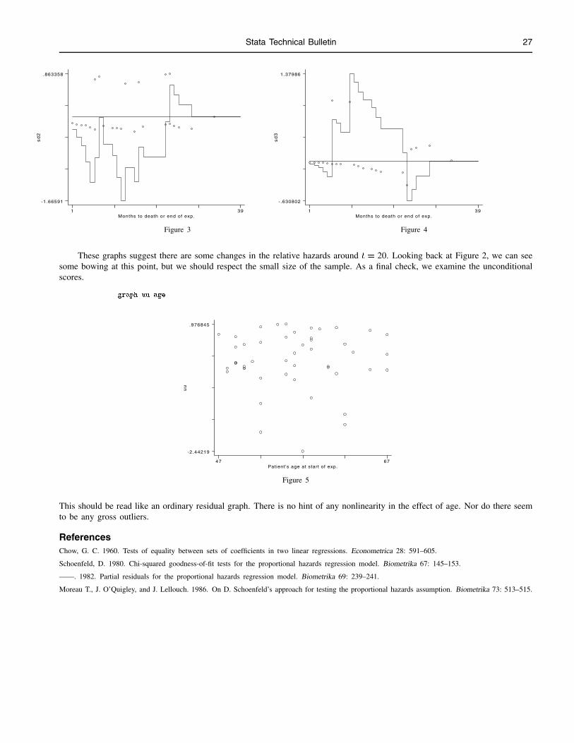
Stata Technical Bulletin 27s
d2
Months to death or end of exp.1 39
-1.66591
.863358
sd
3
Months to death or end of exp.1 39
-.630802
1.37986
Figure 3 Figure 4
These graphs suggest there are some changes in the relative hazards around t = 20. Looking back at Figure 2, we can seesome bowing at this point, but we should respect the small size of the sample. As a final check, we examine the unconditionalscores.
. graph uu age
uu
Patient's age at start of exp.47 67
-2.44219
.976845
Figure 5
This should be read like an ordinary residual graph. There is no hint of any nonlinearity in the effect of age. Nor do there seemto be any gross outliers.
ReferencesChow, G. C. 1960. Tests of equality between sets of coefficients in two linear regressions. Econometrica 28: 591–605.
Schoenfeld, D. 1980. Chi-squared goodness-of-fit tests for the proportional hazards regression model. Biometrika 67: 145–153.
——. 1982. Partial residuals for the proportional hazards regression model. Biometrika 69: 239–241.
Moreau T., J. O’Quigley, and J. Lellouch. 1986. On D. Schoenfeld’s approach for testing the proportional hazards assumption. Biometrika 73: 513–515.
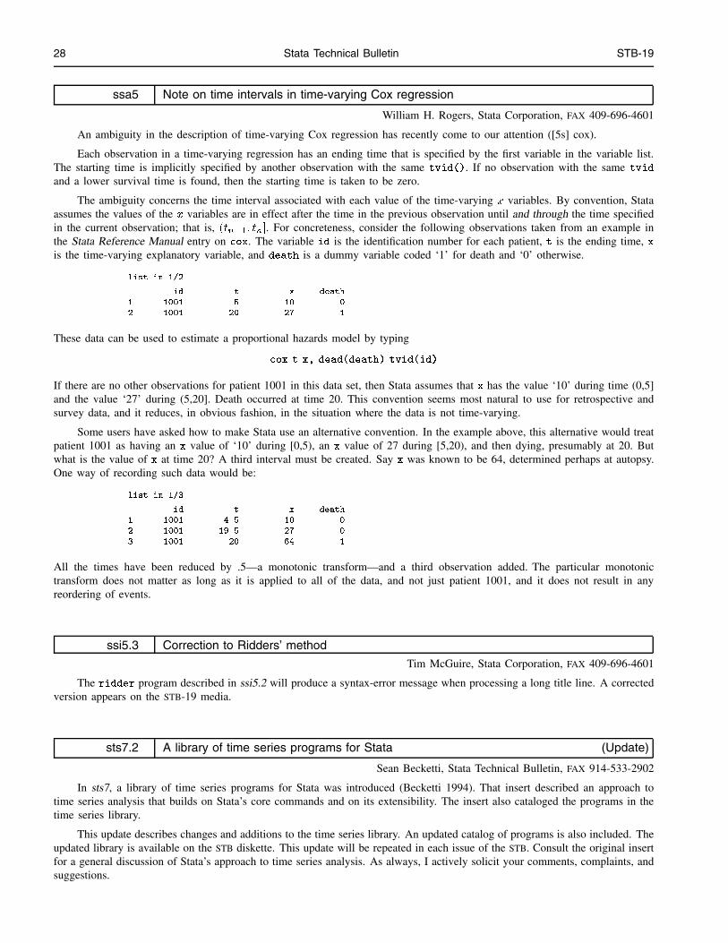
28 Stata Technical Bulletin STB-19
ssa5 Note on time intervals in time-varying Cox regression
William H. Rogers, Stata Corporation, FAX 409-696-4601
An ambiguity in the description of time-varying Cox regression has recently come to our attention ([5s] cox).
Each observation in a time-varying regression has an ending time that is specified by the first variable in the variable list.The starting time is implicitly specified by another observation with the same tvid(). If no observation with the same tvid
and a lower survival time is found, then the starting time is taken to be zero.
The ambiguity concerns the time interval associated with each value of the time-varying x variables. By convention, Stataassumes the values of the x variables are in effect after the time in the previous observation until and through the time specifiedin the current observation; that is, (t
n�1; tn]. For concreteness, consider the following observations taken from an example inthe Stata Reference Manual entry on cox. The variable id is the identification number for each patient, t is the ending time, xis the time-varying explanatory variable, and death is a dummy variable coded ‘1’ for death and ‘0’ otherwise.
. list in 1/2
id t x death
1. 1001 5 10 0
2. 1001 20 27 1
These data can be used to estimate a proportional hazards model by typing
cox t x, dead(death) tvid(id)
If there are no other observations for patient 1001 in this data set, then Stata assumes that x has the value ‘10’ during time (0,5]and the value ‘27’ during (5,20]. Death occurred at time 20. This convention seems most natural to use for retrospective andsurvey data, and it reduces, in obvious fashion, in the situation where the data is not time-varying.
Some users have asked how to make Stata use an alternative convention. In the example above, this alternative would treatpatient 1001 as having an x value of ‘10’ during [0,5), an x value of 27 during [5,20), and then dying, presumably at 20. Butwhat is the value of x at time 20? A third interval must be created. Say x was known to be 64, determined perhaps at autopsy.One way of recording such data would be:
. list in 1/3
id t x death
1. 1001 4.5 10 0
2. 1001 19.5 27 0
3. 1001 20 64 1
All the times have been reduced by .5—a monotonic transform—and a third observation added. The particular monotonictransform does not matter as long as it is applied to all of the data, and not just patient 1001, and it does not result in anyreordering of events.
ssi5.3 Correction to Ridders’ method
Tim McGuire, Stata Corporation, FAX 409-696-4601
The ridder program described in ssi5.2 will produce a syntax-error message when processing a long title line. A correctedversion appears on the STB-19 media.
sts7.2 A library of time series programs for Stata (Update)
Sean Becketti, Stata Technical Bulletin, FAX 914-533-2902
In sts7, a library of time series programs for Stata was introduced (Becketti 1994). That insert described an approach totime series analysis that builds on Stata’s core commands and on its extensibility. The insert also cataloged the programs in thetime series library.
This update describes changes and additions to the time series library. An updated catalog of programs is also included. Theupdated library is available on the STB diskette. This update will be repeated in each issue of the STB. Consult the original insertfor a general discussion of Stata’s approach to time series analysis. As always, I actively solicit your comments, complaints, andsuggestions.
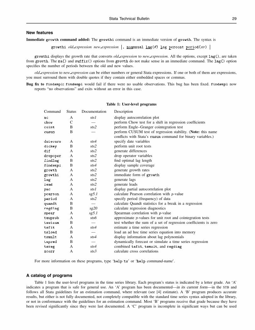
Stata Technical Bulletin 29
New features
Immediate growth command added: The growthi command is an immediate version of growth. The syntax is
growthi old expression new expression�, noannual lag(#) log percent period(str)
�growthi displays the growth rate that converts old expression to new expression. All the options, except lag(), are taken
from growth. The ma() and suffix() options from growth do not make sense in an immediate command. The lag() optionspecifies the number of periods between the old and new values.
old expression to new expression can be either numbers or general Stata expressions. If one or both of them are expressions,you must surround them with double quotes if they contain either embedded spaces or commas.
Bug fix to findsmpl: findsmpl would fail if there were no usable observations. This bug has been fixed. findsmpl nowreports “no observations” and exits without an error in this case.
Table 1: User-level programs
Command Status Documentation Description
ac A sts1 display autocorrelation plotchow C — perform Chow test for a shift in regression coefficientscoint B sts2 perform Engle–Granger cointegration testcusum B — perform CUSUM test of regression stability. (Note: this name
conflicts with Stata’s cusum command for binary variables.)datevars A sts4 specify date variablesdickey B sts2 perform unit root testsdif A sts2 generate differencesdropoper A sts2 drop operator variablesfindlag B sts2 find optimal lag lengthfindsmpl B sts4 display sample coveragegrowth A sts2 generate growth ratesgrowthi A sts2 immediate form of growthlag A sts2 generate lagslead A sts2 generate leadspac A sts1 display partial autocorrelation plotpearson A sg5.1 calculate Pearson correlation with p-valueperiod A sts2 specify period (frequency) of dataquandt B — calculate Quandt statistics for a break in a regressionregdiag B sg20 calculate regression diagnosticsspear A sg5.1 Spearman correlation with p-valuetauprob A sts6 approximate p-values for unit root and cointegration teststestsum B — test whether the sum of a set of regression coefficients is zerotsfit A sts4 estimate a time series regressiontsload B — load an ad hoc time series equation into memorytsmult A sts4 display information about lag polynomialstspred B — dynamically forecast or simulate a time series regressiontsreg A sts4 combined tsfit, tsmult, and regdiag
xcorr A sts3 calculate cross correlations
For more information on these programs, type ‘help ts’ or ‘help command-name’.
A catalog of programs
Table 1 lists the user-level programs in the time series library. Each program’s status is indicated by a letter grade. An ‘A’indicates a program that is safe for general use. An ‘A’ program has been documented—in its current form—in the STB andfollows all Stata guidelines for an estimation command, where relevant (see [4] estimate). A ‘B’ program produces accurateresults, but either is not fully documented, not completely compatible with the standard time series syntax adopted in the library,or not in conformance with the guidelines for an estimation command. Most ‘B’ programs receive that grade because they havebeen revised significantly since they were last documented. A ‘C’ program is incomplete in significant ways but can be used

30 Stata Technical Bulletin STB-19
safely by an advanced Stata user. A ‘D’ program has serious deficiencies, however its code may provide a useful model toadvanced Stata users writing their own time series programs. An ‘O’ program is obsolete, that is, it has been superseded by anewer program. An ‘O’ program is retained if it is still be called by one or two user-level programs. There are currently no ‘D’or ‘O’ programs.
Utilities for time series analysis
Writing programs for time series analysis presents a variety of challenges. In developing this library of programs, I had towrite a pool of utility programs to interpret the time series options, to generate lags, to manipulate the list of variables in a lagpolynomial, and so on. I recommend that you familiarize yourself with these utilities, if you wish to write your own time seriesprograms. A list of some of the most frequently used utility programs appears in Table 2 below.
Table 2: Utility programs
Command Description
ac calculate autocorrelations, standard errors, and Q-statisticsaddl “add” a lag operator to a variable nameaddop “add” an arbitrary operator to a variable namegetrres calculate recursive residuals for a regression modelinlist determine whether a token appears in a token listinvlist determine whether a varname appears in a varlistopnum decode the operators (and their powers) in a varnameparsevl parse a varlist to replace abbreviationssubchar replace one character in a string with anotherts meqn parse a time series command and generate lagsts pars parse a time series command into useful macrosfaketemp generate temporary variable names that can be lagged
Future developments and call for comments
As the comments above indicate, this library of time series programs is under constant revision and extension. Projects underdevelopment include programs to estimate rolling regressions, to estimate vector autoregressions, and to perform maximum-likelihood tests for cointegration. Older programs are being revised to bring them up to Stata’s standards for estimation programs.A disadvantage of these constant revisions is the likelihood of inadvertently introducing errors into the programs. The advantageof constant revision is the ease and rapidity of fixing these errors and the steady increase in Stata’s time series capabilities. Iencourage you to alert me to any errors or inconveniences you find.
If you find an error in any of these commands, I will attempt to correct it by the next issue of the STB. To speed the process,please send me a diskette containing a do-file that replicates the error. Debugging software is similar to auto mechanics: if Ican’t reproduce the problem, I can’t fix it.
ReferenceBecketti, S. 1994. sts7: A library of time series programs for Stata. Stata Technical Bulletin 17: 28–32.
zz3.3 Computerized index for the STB (Update)
William Gould, Stata Corporation, FAX 409-696-4601
The STBinformer is a computerized index to every article and program published in the STB. The command (and entiresyntax) to run the STBinformer is stb. Once the program is running, you can get complete instructions for searching the indexby typing ? for help or ?? for more detailed help.
Stata Technical Bulletin 31
The STBinformer appeared for the first time on the STB-16 distribution diskette and included indices for the first fifteenissues of the STB. The STB-19 distribution diskette contains an updated version of the STBinformer that includes indices for thefirst eighteen issues of the STB. As the original insert stated, I intend to include an updated copy of this computerized index onevery STB diskette. I encourage you to contact me with suggestions for changes and improvements in the program.
ReferenceGould W. 1993. Computerized index for the STB. Stata Technical Bulletin 16: 27–32.
zz4 Cumulative index for STB-13—STB-18
[an] Announcements
STB-13 2 an31 Statement from the new editor S. Becketti
STB-13 3 an32 STB-7—STB-12 available in bound format S. Becketti
STB-14 2 an33 CRC has a new address: : :and a new name A. Humphreys
STB-14 2 an34 Stata 3.1 is available now P. Branton
STB-14 3 an35 A first look at Stata 3.1 S. Becketti
STB-15 2 an36 Stata 3.0 users beware! S. Becketti
STB-16 2 an37 Stata classes and programming services available E. Best
STB-17 2 an38 Stata distributor in France A. Humphreys
STB-17 2 an39 NSF funds workshops on exploratory data analysis for social scientists J. Anagnoson
STB-17 3 an40 Italian translation of Principles of Biostatistics S. Becketti
STB-18 2 an41 STB office moving S. Becketti
[cc] Communications
STB-14 7 cc1 Stata chosen for the Medicare program C. Chapin
STB-17 3 cc2 Running the Stata tutorials on a network A. Reese
[crc] CRC-Provided Support Materials
STB-13 3 crc30 Linearly interpolate (extrapolate) valuesSTB-13 4 crc31 Categorical variable histogramSTB-15 2 crc32 Correction to 3.1 manual description of S MACH
STB-15 2 crc33 Linear spline constructionSTB-17 5 crc34 Programming command: marking observations for inclusionSTB-17 6 crc35 Warning about parity checking on DOS computers
[dm] Data Management
STB-13 6 dm12.1 Selecting claims from medical claims data bases R. Vaughn
STB-13 6 dm13 Person name extraction W. Gould
STB-13 11 dm13.1 String manipulation functions W. Gould
STB-14 8 dm14 Converting Julian dates to Stata elapsed dates C. Chapin
STB-14 10 dm14.1 Converting Stata elapsed dates to Julian dates S. Becketti
STB-16 2 dm15 Interactively list values of variables A. Riley
STB-17 7 dm16 Compact listing of a single variable P. Royston and P. Sasieni
[dt] Data Sets
STB-15 4 dt1 Five data sets for teaching J. T. Anagnoson
[gr] Graphics
STB-15 7 gr13 Incorporating Stata-created PostScript files into TEX/LATEX documentsT. W. Soon and S. L. C. Saw
STB-15 12 gr13.1 \specialfg effects with Stata graphs in TEX documents S. Becketti
[ip] Instruction on Programming
STB-13 13 ip4 Program debugging command S. Becketti
STB-17 8 ip5 A temporary solution to a problem with temporary variable names C. S. Hakkio
[os] Operating System, etc.
STB-17 11 os5.1 Running Intercooled Stata under OS/2 2.1 W. Gould
STB-13 14 os8 Stata and Lotus 1-2-3 P. Royston and W. Gould
32 Stata Technical Bulletin STB-19
STB-13 17 os9 Printing Stata log files S. Becketti
STB-14 10 os10 A method for taking notes during a Stata session B. Rising
STB-14 12 os11 A poor-man’s ‘windowing’ environment for Stata P. Geiger
[qs] Questions and Suggestions
STB-14 12 qs5 How to create stacked bar charts of proportions F. Knaul
STB-14 14 qs6 Query for chemists, physiologists, and pharmacologists P. Geiger
STB-14 14 qs7 Maximum likelihood estimation of Gaussian mixtures I. H. Salgado-Ugarte
[sg] General Statistics
STB-13 18 sg5.1 Correlation coefficients with significance levels S. Becketti
STB-13 18 sg11.2 Calculation of quantile regression standard errors W. Rogers
STB-14 16 sg16.2 GLM: A unified power-link based program including the negative binomial J. Hilbe
STB-16 6 sg16.3 Quasi-likelihood modeling using an enhanced glm command J. Hilbe
STB-16 7 sg16.4 Comparison of nbreg and glm for negative binomial W. Rogers
STB-18 2 sg16.5 Negative binomial regression J. Hilbe
STB-13 19 sg17 Regression standard errors in clustered samples W. Rogers
STB-14 19 sg18 An improved R2 P. Royston
STB-15 13 sg19 Linear splines and piecewise linear functions W. Gould
STB-17 12 sg20 Point biserial correlation J. A. Anderson
STB-17 13 sg21 Equivalency testing R. Goldstein
STB-18 6 sg22 Generalized linear models: revision of glm P. Royston
STB-18 11 sg22.1 Comment on Royston’s revision of glm J. Hilbe
STB-18 13 sg22.2 Certifications of glmr W. Gould
STB-18 15 sg23 Semi-graphical determination of Gaussian components in mixed distributionsI. H. Salgado-Ugarte, M. Shimizu, and T. Taniuchi
STB-18 27 sg24 The piecewise linear spline transformation C. Panis
[snp] Nonparametric Methods
STB-14 22 snp5 The run test for random order S. Becketti
STB-16 8 snp6 Exploring the shape of univariate data using kernel density estimatorsI. H. Salgado-Ugarte, M. Shimizu, and T. Taniuchi
[sqc] Quality Control
STB-17 18 sqc1 Estimating process capability indices with Stata S. L. C. Saw and T. W. Soon
[sqv] Analysis of Qualitative Variables
STB-13 24 sqv8 Interpreting multinomial logistic regression L. Hamilton and C. Seyfrit
[ssi] Simulation and Random Numbers
STB-14 26 ssi4 Confidence intervals in logit and probit models W. Gould
STB-16 20 ssi5 Equation solving by bisection W. Gould
STB-16 23 ssi5.1 Graphing functions W. Gould
STB-17 19 ssi5.2 Equation solving by Ridders’ method T. McGuire
[sss] Social Science and Psychometrics
STB-15 17 sss1 Calculating U.S. marginal income tax rates T. J. Schmidt
[sts] Time Series and Econometrics
STB-13 28 sts3 Cross correlations S. Becketti
STB-15 20 sts4 A suite of programs for time series regression S. Becketti
STB-16 27 sts4.1 More on time series regression S. Becketti
STB-17 22 sts5 Detrending with the Hodrick–Prescott filter T. J. Schmidt
STB-17 25 sts6 Approximate p-values for unit root and cointegration tests C. S. Hakkio
STB-17 28 sts7 A library of time series programs for Stata S. Becketti
STB-18 29 sts7.1 A library of time series programs for Stata (Update) S. Becketti
[zz] Not elsewhere classified
STB-16 27 zz3 Computerized index for the STB W. Gould
STB-17 32 zz3.1 Computerized index for the STB (Update) W. Gould
STB-18 32 zz3.2 Computerized index for the STB (Update) W. Gould


![[ME] Multilevel Mixed Effects - Stata · PDF file[XT] Stata Longitudinal-Data/Panel-Data Reference Manual [ME] Stata Multilevel Mixed-Effects Reference Manual [MI] Stata Multiple-Imputation](https://img.pdfslide.us/doc/110x75/5a78a96c7f8b9a7b698e4b38/me-multilevel-mixed-effects-stata-xt-stata-longitudinal-datapanel-data-reference.jpg)