Solving the Cox Proportional Hazards Model and Its Applications · 2017-05-21 · Abstract Solving the Cox Proportional Hazards Model and Its Applications by Jessica Ko Master of

Solving the Cox Proportional Hazards Model and ItsApplications

Jessica Ko

Electrical Engineering and Computer SciencesUniversity of California at Berkeley

Technical Report No. UCB/EECS-2017-110http://www2.eecs.berkeley.edu/Pubs/TechRpts/2017/EECS-2017-110.html

May 20, 2017

Copyright © 2017, by the author(s).All rights reserved.

Permission to make digital or hard copies of all or part of this work forpersonal or classroom use is granted without fee provided that copies arenot made or distributed for profit or commercial advantage and that copiesbear this notice and the full citation on the first page. To copy otherwise, torepublish, to post on servers or to redistribute to lists, requires priorspecific permission.

Solving the Cox Proportional Hazards Model and Its Applications


by

Jessica Ko

A thesis submitted in partial satisfaction of the

requirements for the degree of

Master of Science

in

Electrical Engineering and Computer Science

in the

Graduate Division

of the

University of California, Berkeley

Committee in charge:

Professor Laurent El Ghaoui, ChairProfessor Aditya Guntuboyina

Spring 2017


Copyright 2017by

Jessica Ko

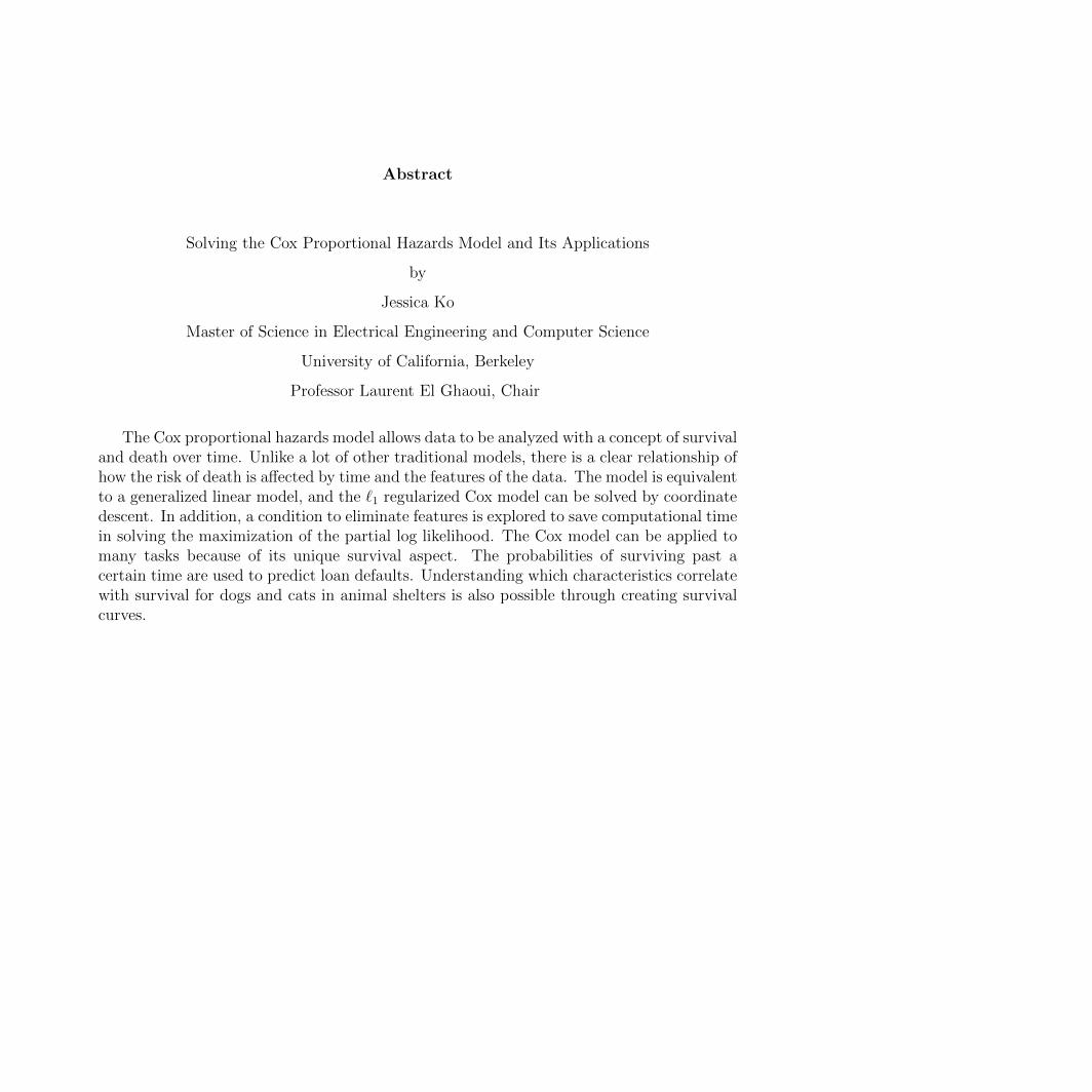
Abstract


by

Jessica Ko

Master of Science in Electrical Engineering and Computer Science

University of California, Berkeley

Professor Laurent El Ghaoui, Chair

The Cox proportional hazards model allows data to be analyzed with a concept of survivaland death over time. Unlike a lot of other traditional models, there is a clear relationship ofhow the risk of death is a↵ected by time and the features of the data. The model is equivalentto a generalized linear model, and the `1 regularized Cox model can be solved by coordinatedescent. In addition, a condition to eliminate features is explored to save computational timein solving the maximization of the partial log likelihood. The Cox model can be applied tomany tasks because of its unique survival aspect. The probabilities of surviving past acertain time are used to predict loan defaults. Understanding which characteristics correlatewith survival for dogs and cats in animal shelters is also possible through creating survivalcurves.

Acknowledgments

I would like to thank my advisor, Professor El Ghaoui, for being supportive, kind, andpatient during my time here at Berkeley. I appreciate all the help and guidance he has givenme throughout my undergraduate and graduate careers. I am glad to have had the oppor-tunity to work with him as I have learned a lot about machine learning and optimization. Ithank him for his valuable advice and comments while I was working on this thesis. I wouldalso like to thank Professor Guntuboyina for reading this work.

I owe endless thanks to my parents, sister, and relatives for their unwavering love, support,and encouragement through this arduous journey. This would not have been possible withoutmy parents, as they have demonstrated how much can be accomplished solely by hard workand passion. I am thankful for my sister who has been a great friend, always believing inme. As cliche as this sounds, there are not enough words to describe how grateful I am forhow much my family has done for me.

i

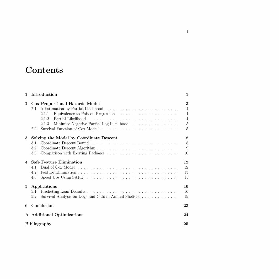
Contents

1 Introduction 1

2 Cox Proportional Hazards Model 32.1 � Estimation by Partial Likelihood . . . . . . . . . . . . . . . . . . . . . . . 4

2.1.1 Equivalence to Poisson Regression . . . . . . . . . . . . . . . . . . . . 42.1.2 Partial Likelihood . . . . . . . . . . . . . . . . . . . . . . . . . . . . . 42.1.3 Minimize Negative Partial Log Likelihood . . . . . . . . . . . . . . . 5

2.2 Survival Function of Cox Model . . . . . . . . . . . . . . . . . . . . . . . . . 5

3 Solving the Model by Coordinate Descent 83.1 Coordinate Descent Bound . . . . . . . . . . . . . . . . . . . . . . . . . . . . 83.2 Coordinate Descent Algorithm . . . . . . . . . . . . . . . . . . . . . . . . . . 93.3 Comparison with Existing Packages . . . . . . . . . . . . . . . . . . . . . . . 10

4 Safe Feature Elimination 124.1 Dual of Cox Model . . . . . . . . . . . . . . . . . . . . . . . . . . . . . . . . 124.2 Feature Elimination . . . . . . . . . . . . . . . . . . . . . . . . . . . . . . . . 134.3 Speed Ups Using SAFE . . . . . . . . . . . . . . . . . . . . . . . . . . . . . 15

5 Applications 165.1 Predicting Loan Defaults . . . . . . . . . . . . . . . . . . . . . . . . . . . . . 165.2 Survival Analysis on Dogs and Cats in Animal Shelters . . . . . . . . . . . . 19

6 Conclusion 23

A Additional Optimizations 24

Bibliography 25

1

Chapter 1

Introduction

Survival analysis is a field dedicated to analyzing the time to the occurrence of an eventof interest. Traditionally, survival analysis is used in bio-statistics to determine the chancesof a patient surviving after undergoing some treatment. For example, this can be applied toanalyzing cancer patients after receiving chemotherapy. Data is recorded from the patientover time, and the outcome after the study is noted. Some possible outcomes are dying,being cured, or exiting the study. However, survival analysis can be applied to other areasto analyze customers leaving over time and recidivism of prisoners once they were released.

One method used in survival analysis is the Cox proportional hazards model or Coxmodel, which uniquely quantifies the risk of the event of interest occurring over time [7].Throughout this work, survival will be considered as when the event of interest did notoccur. In addition, the model can define the e↵ect of features on survival and can determinehow likely the outcome will occur after a certain time for predicting whether an event willoccur. Moreover, features can be investigated to determine if there is a correlation for beingmore likely to occur. In Chapter 2, the theory behind the Cox model will be described.

Throughout this work, the `1 norm is added to the Cox proportional hazards modelbecause regularization encourages sparsity and prevents overfitting. Then, cyclic coordinatedescent is used to solve this problem. Previous work has been done on using coordinatedescent for solving the Cox proportional hazards model with elastic net, which is implementedin R. Cyclic coordinate descent is shown to be successful for convex problems with `1, `2, orelastic net penalties because it exploits the sparsity of the model and has an explicit formfor each coordinate-wise maximization [11]. Furthermore, cyclic coordinate descent is ane�cient algorithm for the regularized Cox model [20]. Coordinate descent has been provento be useful for solving other models such as elastic-net penalized regression models [13, 26].In Chapter 3, a cyclic coordinate descent method for solving a regularized Cox model willbe explained, and its higher accuracy compared to existing methods will be discussed.

In addition, safe feature elimination (SAFE) is applied to the model to speed up thecomputation of solving the model in Chapter 4. Applying SAFE to the Lasso problem hasshown to reduce running time [9]. The computational e↵ort of the feature elimination stepis negligible compared to solving the Lasso problem. Furthermore, SAFE can be applied on

CHAPTER 1. INTRODUCTION 2

other `1 penalized convex problems like the Cox model.After the Cox model is solved, the model can be used for a variety of applications.

Chapter 5 provides applications of the Cox model for two scenarios. Predicting defaults onloans and analyzing characteristics of animals with di↵erent outcomes in animal shelters aresuccessful using the Cox model.

3

Chapter 2

Cox Proportional Hazards Model

The Cox proportional hazards model accurately depicts interactions between the featuresand risk in the hazard function [7]. Time-dependent features can also be easily used in themodel to account for features that may change with time. Even though time-dependentfeatures are not considered in this work, they are powerful for creating a model that preciselydescribes the interactions of the features. Given a vector x 2 Rd of d features and a parameter� 2 Rd, the hazard function is defined as

�(t|x) = �0(t)e�

>x

.

The baseline hazard function �0(t) does not need to be specified for the Cox model,making it semi-parametric. This is advantageous because the Cox model will be robustand have fewer restrictions. The baseline hazard function is appropriately named becauseit describes the risk at a certain time when x = 0, which is when the features are notincorporated. The hazard function describes the relationship between the baseline hazardand features of a specific sample to quantify the hazard or risk at a certain time.

The model only needs to satisfy the proportional hazard assumption, which is that thehazard of one sample is proportional to the hazard of another sample [6]. This property canbe checked by using p-values of the Cox model as described in Chapter 5. Two samples x1

and x2 satisfy this assumption when the ratio is not dependent on time as shown below.

�(t|x1)

�(t|x2)=

�0(t)e�>x1

�0(t)e�>x2

=e

�

>x1

e

�

>x2

Also, more generally the relative risk to the average risk of the training data is definedbelow for sample x

k

and sample mean x.

�(t|xk

)

�(t|x) =�0(t)e�

>x

k

�0(t)e�>x

=e

�

>x

k

e

�

>x

CHAPTER 2. COX PROPORTIONAL HAZARDS MODEL 4

2.1 � Estimation by Partial Likelihood

The parameter � can be found by maximizing the partial likelihood because the hazardfunction is not specified. The following sections explain the formulation of the optimizationproblem. In order to be used for the Cox model, each sample i needs:

• x

i

a feature vector;

• T

i

time when event occurred or the censoring time, which is the last time the sampleis observed if the event of interest did not occur in the time period;

• D

i

death indicator where 1 is for when death occurred and 0 is for censoring

2.1.1 Equivalence to Poisson Regression

The partial likelihood of the Cox model can be fitted by the likelihood of Poisson regres-sion, a generalized linear model, because the likelihoods are proportional to each other [25].The advantage of the estimates of � being the same is that it can be fitted using softwarefor generalized linear models like in R. Alternatively, the estimate from the Cox model canbe used for Poisson regression. In Chapter 3, a coordinate descent method is proposed forsolving the maximum partial likelihood of the Cox model.

The Cox model can be interpreted in terms of a Poisson regression. Given the cumulativehazard ⇤(t) and sample i, the estimates of � can be obtained by treating the death indicatorD

i

as Poisson distributed with mean µ

i

= ⇤(ti

)e⌘i where ⌘ = �

>x. The link function is

modified to be �

>x = log(µ

i

) � log(⇤(ti

)) [16]. More information about the cumulativehazard is in Chapter 2.2.

2.1.2 Partial Likelihood

In order to formulate the partial likelihood, the f unique failure times are ordered in-creasingly t1 < · · · < t

f

and j(i) is the index of the sample failing at time t

i

. When at mostone sample failed at each time, the partial likelihood for the Cox model can be written as

L(�) =fY

i=1

�0(ti)e�>x

j(i)

Pj2R

i

�0(ti)e�>x

j

=fY

i=1

e

�

>x

j(i)

Pj2R

i

e

�

>x

j

where the risk set R

i

is the set of indices of samples with death or censor times occurringafter t

i

or Ri

= {k|Tk

� t

i

}. This represents the probability of failure occurring to a sampleat time t

i

among those at risk at time t

i

. The semi-parametric property can be exhibitedhere because the baseline hazard �0 gets canceled out.


However, the partial likelihood above does not take tied events into account, so theprobabilities are not as accurate. Tied events occur if the number of deaths d

i

at time t

i

isgreater than 1. Breslow introduces a di↵erent partial likelihood function to deal with theties [5]. Given that I(i) is the set of indices where a sample fails at time t

i

or I(i) = {k|Dk

=1 and T

k

= t

i

}, the partial likelihood can be redefined as shown below.

L(�) =fY

i=1

e

(P

s2I(i) �>x

s)⇣P

j2Ri

e

�

>x

j

⌘d

i

This work will refer to the Breslow ties version as the partial likelihood because ties oftenoccur in the datasets.

2.1.3 Minimize Negative Partial Log Likelihood

The parameter � can be found by minimizing the negative partial log likelihood `(�),which is defined below.

`(�) = log(L(�))

=fX

i=1

loge

Ps2I(i) �

>x

s

⇣Pj2R

i

e

�

>x

j

⌘d

i

=fX

i=1

2

4

0

@X

s2I(i)

�

>x

s

1

A� d

i

logX

j2Ri

e

�

>x

j

3

5

The minimization of the negative log likelihood with `1 regularization is formed below inthe optimization problem with objective f(�).

f(�) = �`(�) + �k�k1

min�

f(�) (2.1)

Regularization is included because there are many benefits such as being more accuratethan stepwise selection and yielding interpretable models [22]. In addition, the regularizationprevents degenerate behavior when there are more predictors than observations.

2.2 Survival Function of Cox Model

The survival function obtained from the Cox model can be used to make predictions on asample surviving because it’s the probability of a sample surviving after time t. The survivalfunction is defined as


S(t) = exp (�⇤(t)).

The cumulative hazard or cumulative risk ⇤(t) is defined as

⇤(t) =

Zt

0

�(s)ds

where �(t) is the hazard function, the instantaneous probability of death at time t, givensurvival until t [18]. It can also be rewritten as

�(t) = � d

dt

logS(t).

The survival function can be rewritten at time t for a given sample x

S(t|x) = exp(�⇤(t)) = exp

✓�Z

t

0

�(s|x)ds◆

= exp

✓�Z

t

0

�0(s)e�

>x

ds

◆

= exp

✓�e�>

x

Zt

0

�0(s)ds

◆

= S0(t)e

�

>x

where the cumulative baseline hazard is ⇤0(t) =R

t

0 �0(s)ds and the baseline survival functionis S0(t) = e

�⇤0(t) [19] . The survival function S(t|x) or probability of survival after time t

is defined by S0(t)e�

>x

. The parameter � can be recovered by a coordinate descent methoddiscussed in Chapter 3. Although the hazard function is not needed for the parameterestimation by partial likelihood, it is necessary to find the survival function for prediction.In the following sections, two methods for estimating the cumulative baseline hazard ⇤0(t)will be discussed.

Breslow Estimator

The Breslow estimator of the cumulative baseline hazard is defined below [15].

⇤0(t) =X

i:Ti

t

d

iPj2R

i

e

�

>x

j

(2.2)

The cumulative hazard is estimated by using the expected number of failures in a timeperiod (t, t+ �t).


d

i

⇡ �t

X

j2Ri

�0(t)e�

>x

j

�t�0(ti) ⇡d

iPj2R

i

e

�

>x

j

By summing over the times, the cumulative hazard function is derived to show Equation 2.2[27].

Weibull Distribution

The hazard function can be estimated by the Weibull distribution �0(t) ⇠ Weibull(�, k)[21].

�0(t) = (�k)(�t)k�1

The cumulative hazard function can then be written as

⇤0(t) = 1� e

�(�t)k.

The hazard or risk is increasing when k > 1, so deaths or failures are more likely to occuras time progresses. Similarly, hazard or risk is decreasing when k < 1.

After the parameter � and the cumulative baseline hazard is estimated, the probability ofsurviving after time t or the survival function can be recovered. The probability of survivalafter time t can be used for predictions by considering samples where S(t) > 0.5 as surviving.Chapter 5 shows an application of using survival functions to predict loan defaults.

8

Chapter 3

Solving the Model by CoordinateDescent

Cyclic coordinate descent is used to solve the minimum partial log likelihood with the `1norm. Throughout this chapter, it is assumed that the `1 norm is included in the optimizationproblem as shown in Equation 2.1. The separability structure of the cost function, wherethe partial log likelihood `(�) is di↵erentiable and convex and k�k1 is convex, guaranteesthat the coordinate descent algorithm will converge to the optimal solution [23, 24]. Thealgorithm cycles between fixing each index and solving the minimization problem. Eachindividual problem is written as below where f

k

is the objective function corresponding tofixing all indices of � except for k.

min�

k

f

k

(�k

)

Each individual minimization problem for a fixed index is solved by the bisection method.The benefit of this method is that calculating the derivative with respect to one variable isnot as costly as calculating the gradient [8].

3.1 Coordinate Descent Bound

The method starts with an interval where the optimal index k of the parameter �⇤k

fallsunder. A lower bound L and upper bound U can be found such that �

⇤k

2 [Lk

, U

k

] andL

k

U

k

. Using some guidelines, it is possible to find bounds for the optimal parameter.Property 1. If f 0

k

(Lk

) < 0 < f

0k

(Uk

), then �

⇤k

2 [Lk

, U

k

] and L

k

U

k

.Proof : f

k

(�k

) is a convex function, so the derivative is monotonically increasing. Lk

U

k

because f

0k

(Lk

) f

0(Uk

). The derivative of a convex function is continuous, so by theIntermediate Value Theorem, 9�⇤

k

such that f

0k

(�⇤k

) ⇡ 0 and �

⇤k

2 [Lk

, U

k

]. The globalminimum is found at this critical point.

When the bound, Lk

and U

k

, can be found for all indices k of �, Property 1 can be used.The first estimate can be a number closer to 0 because the `1 regularization will likely cause

CHAPTER 3. SOLVING THE MODEL BY COORDINATE DESCENT 9

the parameters to be sparse. A simple guideline is to set the bounds so that Lk

< 0 < U

k

.The bounds can be continually doubled until Property 1 is satisfied.

However, it is possible that f 0k

(�k

) < 0 or f 0k

(�k

) > 0 for all �i

and Property 1 will neverbe satisfied. In this case, when the bounds get su�ciently large, then a bound cannot bedefined precisely and the optimal values likely lie close to infinity. The heuristics used tofind a bound for coordinate descent are shown in Algorithm 1.

for index k in � doinitialize L

k

, U

k

where L

k

< 0 < U

k

;while U

k

� L

k

< Max Limit and ( f

0k

(Lk

) � 0 or f

0k

(Uk

) 0 ) doif f

0k

(Lk

) � 0 thenL

k

2Lk

;endif f

0k

(Uk

) 0 thenU

k

2Uk

;end

endend

Algorithm 1: Optimal �k

Bound

3.2 Coordinate Descent Algorithm

After finding the bound for the optimal �, coordinate descent and the bisection methodcan be used on the model. For coordinate descent, all indexes in � are fixed except �

k

. Thederivative of the objective function, f 0

k

(�k

), with respect to index k where x

s,t

indicates thet feature of sample s is defined by Equation 3.1 . Because the `1 is not di↵erentiable at 0, asubgradient is introduced to handle this case [4] . Thus, the subgradient of kxk1 = g(x).

g(x) =

(+1, if x > 0

�1, otherwise

Using this as the subgradient for `1 norm, the following can be defined as

f

0k

(�k

) =d

d�

k

[�`(�) + �k�k1]

=fX

i=1

2

4

0

@X

s2I(i)

x

s,k

1

A�

d

iPj2R

i

e

�

>x

j

! X

j2Ri

x

j,k

e

�

>x

j

!3

5+ �g(�k

). (3.1)

The bisection method will attempt to find � such that f 0(�⇤) ⇡ 0. The full algorithm isshown in Algorithm 2.


initialize � ;while � Not Converged do

for index k in � doFix all indexes except i in �;Consider interval [L

k

, U

k

] 2 �

⇤k

;l L

k

;u U

k

;while �

k

Not Converged dox (l + u)/2 ;if f

0k

(x) < 0 thenl x ;

elseu x ;

endend�

i

x;end

endAlgorithm 2: Coordinate Descent

In Appendix A, more optimizations can be included to speed up computation time bywriting the equations in matrix form and caching values.

3.3 Comparison with Existing Packages

In this section, there is a brief comparison of the coordinate descent algorithm mentionedin this chapter to existing packages in R. The survival package in R contains a functioncoxph that also fits data to the Cox model, but the model is not regularized. This R packagewill not be as good for sparse data and may tend to overfit.

While the survival package does not have the regularization term, the glmnet packageincludes the regularization term in the form of elastic net, which includes the `1 and `2 norm[12]. In addition, glmnet can solve other generalized linear models. Using 12,000 sampleswith 14 features from the loan dataset that will be explored in Chapter 5, the glmnet packageperforms very fast in less than one second for any value of �, but the coordinate descentmethod ranges from a few seconds to about one minute using L

k

= �10 and U

k

= 10 for allindices. The exact timings of the coordinate descent method are described in more detailin Table 4.1. However, for glmnet, accuracy in the minimizing the negative log likelihood issacrificed for faster computation times.

The objective function values shown in Table 3.1 are obtained by solving the Cox modelwith glmnet or the coordinate descent method and computing the objective function valuesusing the optimal parameter. The glmnet package seems to aggressively zero out many


indices, which may lead to its reduced accuracy. This e↵ect is noticeable in the table becausethe objective function value is the same for � � 0.5.

Table 3.1: Compare Objective Function of glmnet and Coordinate Descent

� glmnet Coordinate Descent0 51695.84 51120.600.5 51536.44 51121.2310 51536.44 51128.5250 51536.44 51153.70100 51536.44 51179.85

The coordinate descent method achieves better accuracy by getting a smaller value forthe objective function at optimum at the expense of a longer computation time. The longercomputation time can be justified because the model only needs to be fit to the data oncefor every � value.

12

Chapter 4

Safe Feature Elimination

By forming the dual of the Cox model, safe feature elimination (SAFE) can be applied tothe model to eliminate features that are not present after solving the optimization problem.Performing the feature elimination has many computation benefits because it can greatlyreduce the time needed to solve the optimization problem. The feature elimination stepcan be parallelized because each feature can be screened independently of each other. Inaddition, each elimination step requires significantly little computation to perform. Thismethod of feature elimination is shown to be very beneficial for `1-penalized least-squareregression problems [9].

4.1 Dual of Cox Model

In order to define the dual, the optimization problem for the Cox model can be rewritten,assuming the data is in a matrix X = [x1, . . . , xn

] 2 Rd⇥n for n samples and � 2 Rd. Afailure times matrix can be defined as � := (�

ij

) 2 {0, 1}f⇥n where f is the number of uniquefailure times and �

ij

= 1 if j 2 R

i

.Assuming Z = 1�>

X 2 Rf⇥n such that Z

ij

= �

>x

j

for every i where 1 is a vector ofones in Rf , the maximization problem from Chapter 2 can be rewritten as

p

⇤ = max�,Z

c

|� �

fX

i=1

d

i

log

X

j2Ri

e

Z

ij

!� �k�k1

= max�,Z

c

|� �

fX

i=1

d

i

log

nX

j=1

�

ij

e

Z

ij

!� �k�k1

where c =X

{i|Di

=1}

x

i

2 Rd.

CHAPTER 4. SAFE FEATURE ELIMINATION 13

Using a dual variable U 2 Rf⇥n, the dual can be written as

p

⇤ = minU

max�,Z

c

|� �

fX

i=1

d

i

log

nX

j=1

�

ij

e

Z

ij

!� �k�k1 + TrU>(Z � 1�>

X). (4.1)

Using U

> = [u1, . . . , uf

] and Z

> = [z1, . . . , zf ] where u

i

, z

i

2 Rn, the trace can be rewritten

TrU>Z =

fX

i=1

u

|i

z

i

.

The dual problem can be rewritten as

p

⇤ = minU

fX

i=1

maxz

i

u

|i

z

i

� d

i

log

nX

j=1

�

ij

e

Z

ij

!: kXU

>1� ck1 �.

For each i, consider each optimization problem

maxz

i

u

|i

z

i

� d

i

log

nX

j=1

�

ij

e

Z

ij

!: kXU

>1� ck1 �.

The solution is

=

8><

>:d

i

nX

j=1

U

ij

logUij

if ui

� 0,1>u

i

= 1, 8 j : u

ij

(1��ij

) = 0,

+1 otherwise

where �j

is the jth column of �. The dual can then be written as

p

⇤ = minU

fX

i=1

d

i

nX

j=1

U

ij

logUij

: kXU

>1� ck1 �, U1 = 1, U � 0, U �� = 0

where � represents element-wise multiplication.

4.2 Feature Elimination

After the dual is formed, the criteria for the safe feature elimination can be derived. Foreach feature k = 1, . . . , d, if the following holds, then �

k

= at optimum where f

k

is the kthrow of X.

� > maxU

|f>k

U

>1� c

k

| : U1 = 1, U � 0, U �� = 0 (4.2)

This can be shown by looking at Equation 4.1 to get �⇤k

= 0 the following must be true atoptimum

��|�⇤k

|+ (f>k

U

>1� c

k

)�⇤k

< 0. (4.3)


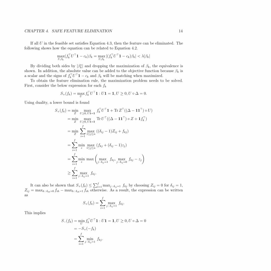
If all U in the feasible set satisfies Equation 4.3, then the feature can be eliminated. Thefollowing shows how the equation can be related to Equation 4.2.

maxU,�

k

(f>k

U

>1� c

k

)�k

= maxU,�

k

|(f>k

U

>1� c

k

)�k

| < �|�k

|

By dividing both sides by |�⇤k

| and dropping the maximization of �k

, the equivalence isshown. In addition, the absolute value can be added to the objective function because �

k

isa scalar and the signs of f>

k

U

>1� c

k

and �

k

will be matching when maximized.To obtain the feature elimination rule, the maximization problem needs to be solved.

First, consider the below expression for each f

k

S+(fk) = maxU

f

>k

U

>1 : U1 = 1, U � 0, U �� = 0.

Using duality, a lower bound is found

S+(fk) = minZ

maxU�0, U1=1

f

>k

U

>1+ TrZ>((�� 11>) � U)

= minZ

maxU�0, U1=1

TrU>((�� 11>) � Z + 1f>k

)

= minZ

fX

i=1

max1jn

((�ij

� 1)Zij

+ f

kj

)

=fX

i=1

minz

max1jn

(fkj

+ (�ij

� 1)zj

)

=fX

i=1

minz

max

✓max

j : �ij

=1f

kj

, maxj : �

ij

=0f

kj

� z

j

◆

�fX

i=1

maxj : �

ij

=1f

kj

.

It can also be shown that S+(fk) P

f

i=1 maxj : �

ij

=1 f

kj

by choosing Z

ij

= 0 for �ij

= 1,Z

ij

= maxh : �

ih

=0 fih �maxh : �

ih

=1 fih otherwise. As a result, the expression can be writtenas

S+(fk) =fX

i=1

maxj : �

ij

=1f

kj

.

This implies

S�(fk) = minU

f

>k

U

>1 : U1 = 1, U � 0, U �� = 0

= �S+(�fk)

=fX

i=1

minj : �

ij

=1f

kj

.


Using these two expressions, Equation 4.2 can be written as

� > max (|S+(fk)� c

k

|, |S�(fk)� c

k

|)

� > max

c

k

�fX

i=1

minj : �

ij

=1X

kj

,

fX

i=1

maxj : �

ij

=1X

kj

� c

k

!. (4.4)

If the kth feature satisfies the SAFE condition (Equation 4.4), then �

k

= 0 at optimum.

4.3 Speed Ups Using SAFE

The feature elimination is computationally faster than not using SAFE because manycomputations are saved. The SAFE condition only needs to be checked once for every featurein the beginning of the optimization. In addition, the SAFE condition is very quick to checkbecause of the form of the expression. An experiment was run on 12,000 samples with14 features from the loan dataset that will be explored in Chapter 5. The results of thetimings with and without the SAFE condition are shown in Table 4.1. For these times, thecoordinate descent bound is chosen to be [�10, 10] for each index. The computations arerun on a machine with 8 GB of memory and an 2.6GHz dual-core Intel Core i5 processor.

With smaller values of �, the model does not eliminate as many features, so using SAFEis only 16% faster than not using SAFE for solving the minimization problem. However,when the regularization weight is larger and more features are eliminated, there is significantcomputation advantage. As shown in the table, the largest regularization weight performs442% faster when using the SAFE conditions. Using safe feature elimination will speed upthe time it takes to solve the optimization problem especially when the regularization weightsare larger.

Table 4.1: Timing Computations with and without SAFE in Seconds

� No SAFE SAFE% Faster

Using SAFE# Features Satisfying

SAFE Condition0.0001 131.0 109.70 19.42% 20.5 116.29 99.77 16.56% 210 107.5 92.49 16.23% 250 77.42 65.84 17.59% 3100 71.35 33.85 110.78% 4200 36.48 15.79 131.03% 7300 30.41 5.61 442.07% 9

16

Chapter 5

Applications

In this chapter, the Cox model will be applied to two di↵erent datasets: predictingloan defaults and investigating the relationship of characteristics of animals in shelters andsurvival. In order for the Cox model to be applicable to a dataset, there needs to be a cleardefinition of elapsed time and what event is considered to be death or failure. The followingdatasets have both properties, so the Cox model can be applied to these tasks. Both of theseapplications solve the regularized Cox model by using coordinate descent with SAFE.

5.1 Predicting Loan Defaults

Deciding whether or not to approve a loan is important for banks because issuing loansthat are likely to default are risky and decrease the bank’s profitability. By using the Coxmodel to aid in predicting loan defaults, banks can make a better decision about issuingloans. In addition, this will help borrowers financially plan by allowing them to understandhow likely they can get a loan. Furthermore, this can be applied to loans on Lending Clubto help investors discover good investments by finding loans that are less likely to default.Lending Club is one of the world’s largest online credit marketplace that allows for peer-to-peer lending.

In the following sections, the dataset on loans issued from 2007 to 2016 is used forpredicting loan defaults, a binary task [14]. The dataset contains about one million samplesand 110 features, but only 15,000 samples and a subset of features will be used for thepredictions. The training, validation, and testing sets were split so that the two classes arebalanced.

Data

The time period was calculated by finding the number of months that have passed sincethe loan was issued and when the last payment was received. Even though loans are issuedon di↵erent dates, all the start dates can be assumed to be the same time without loss of

CHAPTER 5. APPLICATIONS 17

generality [25]. Failure of the loan is defined as ’Charged O↵’, ’Default’, or ’Does not meetthe credit policy. Status:Charged O↵’.

The loan default dataset contains many features, and a subset of these features wasselected to use for prediction. First, the features were preprocessed. Features with continu-ous values were normalized into their z-scores like annual income, and categorical variableswere one-hot encoded like home ownership. The following features were selected and theirdescriptions from the dataset are shown [14]

• ’annual inc’: Self-reported annual income.

• ’dti’: A ratio calculated using the borrowers’ total monthly debt payments on the totaldebt obligations, excluding mortgage and the requested Lending Club loan, divided bythe borrowers self-reported monthly income.

• ’emp length’: Employment length in years. Possible values are between 0 and 10 where0 means less than one year and 10 means ten or more years.

• ’funded amnt’: The total amount committed to that loan at that point in time.

• ’grade’: Lending Club assigned loan grade (’A’, ’B’, ’C’, ’D’, ’E’, ’F’, or ’G’)

• ’home ownership’ : Home ownership status of the borrower such as own, rent, mort-gage, or other.

• ’int rate’: Interest rate of loan

• ’loan amnt’ : Listed amount of the loan applied for by the borrower. The creditdepartment can reduce the loan amount.

• ’mort acc’: Number of mortgage accounts.

• ’num bc sats’: Number of satisfactory bankcard accounts.

• ’num bc tl’: Number of bankcard accounts.

• ’pub rec bankruptcies’: Number of public record bankruptcies.

• ’revol bal’: Total credit revolving balance.

• ’term’: Number of payments on the loan can either be 36 or 60 months.

In order to use the Cox model, the proportional hazard assumption must hold for the data.The assumption can be verified with a p-value < 0.05 for the features selected using coxph inR. Using this assumption, there are 14 features selected : ’dti’, ’emp length’, ’funded amnt’,’grade = C’, ’grade = D’, ’grade = F’, ’home ownership=OWN’, ’home ownership=OTHER’,’int rate’, ’mort acc’, ’num bc sats’, ’num bc tl’, ’pub rec bankruptcies’, and ’term= 36months’.


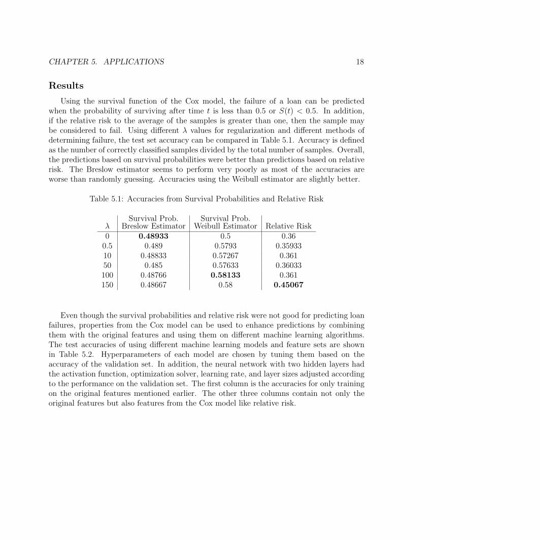
Results

Using the survival function of the Cox model, the failure of a loan can be predictedwhen the probability of surviving after time t is less than 0.5 or S(t) < 0.5. In addition,if the relative risk to the average of the samples is greater than one, then the sample maybe considered to fail. Using di↵erent � values for regularization and di↵erent methods ofdetermining failure, the test set accuracy can be compared in Table 5.1. Accuracy is definedas the number of correctly classified samples divided by the total number of samples. Overall,the predictions based on survival probabilities were better than predictions based on relativerisk. The Breslow estimator seems to perform very poorly as most of the accuracies areworse than randomly guessing. Accuracies using the Weibull estimator are slightly better.

Table 5.1: Accuracies from Survival Probabilities and Relative Risk

�

Survival Prob.Breslow Estimator

Survival Prob.Weibull Estimator Relative Risk

0 0.48933 0.5 0.360.5 0.489 0.5793 0.3593310 0.48833 0.57267 0.36150 0.485 0.57633 0.36033100 0.48766 0.58133 0.361150 0.48667 0.58 0.45067

Even though the survival probabilities and relative risk were not good for predicting loanfailures, properties from the Cox model can be used to enhance predictions by combiningthem with the original features and using them on di↵erent machine learning algorithms.The test accuracies of using di↵erent machine learning models and feature sets are shownin Table 5.2. Hyperparameters of each model are chosen by tuning them based on theaccuracy of the validation set. In addition, the neural network with two hidden layers hadthe activation function, optimization solver, learning rate, and layer sizes adjusted accordingto the performance on the validation set. The first column is the accuracies for only trainingon the original features mentioned earlier. The other three columns contain not only theoriginal features but also features from the Cox model like relative risk.


Table 5.2: Accuracies of Models Using Di↵erent Features

ModelOriginal Features

OnlyRelative Risk

from Cox ModelSurvival Prob.from Cox Model

Risk and Prob.from Cox Model

Logistic Regr. 0.66367 0.66067 0.664 0.66367SVM 0.588 0.591 0.589 0.59167

Decision Tree 0.67667 0.68967 0.68767 0.66867Random Forest 0.66067 0.66633 0.66833 0.66367Neural Network 0.65633 0.65367 0.65733 0.65667

Overall, the features from the Cox model, relative risk and survival probabilities, slightlyincreased the accuracy of predicting the loan failures. Even though the survival probabilitieswere bad predictors on their own, combining them with the original features improved theaccuracy. This is shown when comparing the accuracies of only using the original featureswith the accuracies of also using Cox model features. When comparing the di↵erent models,the decision tree performs the best across the di↵erent feature sets. Further improvementsin the accuracy can possibly be made by using the Cox model in the loss function of a neuralnetwork [2].

5.2 Survival Analysis on Dogs and Cats in AnimalShelters

Animal shelters are often overcrowded with animals because they lack the resources tocare for homeless pets and more people disown their pets than adopt them. In this section,correlations between animal characteristics and survival once entering an animal shelter overtime will be explored. Understanding these correlations can help improve animal shelters andthe well-being of these animals. Many di↵erent factors can a↵ect the survival of animals inpet shelters. In order to understand the correlations between these features like color, breed,and etc. on survival, an appropriate model like the Cox model must be used. Survivalanalysis is applied on the Austin Animal Shelter dataset to explore survival of animalsin shelters [1]. The Austin Animal Shelter operates the largest No Kill municipal animalshelter in the United States. Even though the animals are not killed for population control,overcrowding can still be a problem if there are too many animals in the shelter and notenough resources to care for them in the facilities.

The dataset contains 49,970 animals recorded from 2013 to 2016 such as outcome time,outcome type (adoption, transfer, euthanasia, or death), and etc. Even though the animalshave di↵erent dates for when they entered the animal shelter, the start times can be inter-preted as starting at the same with no loss of generality [25] . The time is measured as thedi↵erence between intake time and outcome time. The animal shelter collected a variety


of categorical features like intake type (Owner, Stray, or PublicAssist), injured/sick or not,pregnant or not, dog or cat, spayed/neutered or not, gender, purebred or mix, and black col-ored or not. Similar to Chapter 5.1, features satisfying the Cox proportionality assumptioncan only be used, so this reduces the feature set to only spayed/neutered or not, gender,and black colored or not. For this dataset, survival is defined as an animal being adoptedor transferred to another center. Failure, or death, is defined as when an animal dies or iseuthanized.

In order to graph the survival curves, the best regularization weight � needs to be chosen.Unlike classification tasks, there is not a well defined accuracy metric to pick the best � value,so another metric must be used. The � with the lowest cross-validated deviance is chosenfor the model [17]. The deviance is calculated by doing 10-fold cross validation. Figure 5.1shows how the deviances slowly increases as log(�) increases, so log(�) = �8.9 is chosen.

Figure 5.1: Picking the Best �

After finding � by coordinate descent and SAFE, the survival curves can now be graphedto compare the di↵erence in the survival probabilities for certain features. For the feature ofinterest, the data is separated by the feature values. For example, the data is separated bymale and female for gender. After, the mean x of each feature is calculated, and the indexof the feature is marked as the respective value. For example, if gender is feature i, thenx1[i] = 1 for female and x0[i] = 0 for male. The two mean vectors, one for each binary class,are then graphed using the survival function S(t|x0) or S(t|x1) for all failure times with theBreslow estimator for the cumulative baseline hazards. The survival curves for the three


features are shown in Figures 5.2, 5.3, and 5.4. Each downward step in the graphs indicatesan event of failure.

Figure 5.2:

Figure 5.3:


Figure 5.4:

Figure 5.2 shows that spayed or neutered animals correlate more with survival. Peoplemay be more likely to adopt a pet who has undergone this procedure because it can savecosts and help curb overpopulation. Figure 5.3 shows that black colored animals correlatewith lower survival. Black cats are sometimes symbolized as bad luck, and darker coloreddogs are often portrayed as being aggressive in media. This observation may be relatedto black dog syndrome, which is a tendency for black dogs to be adopted less frequently.Compared to the other factors, gender does not seem to correlate with survival as greatly asshown in Figure 5.4.

Because other features did not satisfy the proportional hazards assumption, they couldnot be analyzed with the model and limited what kind of features could be explored, eventhough there are several other features available in the dataset like breed and intake type.The modified version, the stratified general Cox, could adjust those features that do notsatisfy the proportional hazards assumption [3]. More work can be done in the future toincorporate more features for the model.

23

Chapter 6

Conclusion

In this work, the Cox proportional hazards model with `1 regularization is solved by co-ordinate descent with the bisection method. Through experiments, this method is more ac-curate but slower in computations compared to other methods. The safe feature eliminationstep reduces the running time of solving the model without introducing long computationsto perform the step.

The Cox model may be used for many applications because of the relationship betweenthe risk of an event over time and features of the sample. Predicting loan defaults is exploredwith the Cox model by using the survival function. Even though the survival function itselfperformed poorly, using the Cox model for feature engineering such as the relative risk andsurvival function is e↵ective in increasing the classification accuracy compared to modelsthat do not use these features. In addition, the Cox model is used to explore how featuresa↵ect the survival of animals in animals shelters. Certain characteristics of animals such asnot being black colored and being spayed or neutered correlate to survival.

While solving the regularized Cox proportional hazards model with coordinate descentfor its applications was successful, there are still many improvements and explorations to bemade. Converging safe regions are shown to lead to faster convergence for Lasso and canpossibly be explored for the Cox model [10]. To deal with features that do not satisfy theproportional hazards assumption, the stratified Cox model can be used, so the feature setcan be expanded [3]. The Cox model can also be incorporated into the loss function of aneural network to further improve accuracies [2].

24

Appendix A

Additional Optimizations

In order to save addition computation, the model can be written in matrix form. Thedata is assumed to be X 2 Rn⇥d for n samples and d features and � 2 Rd. �

R

2 Rf⇥n is amatrix where �

R

ij

= 1 if sample j failed at the time corresponding to index i and f is thenumber of unique times a sample failed. �

F

2 Rn⇥1 is a matrix where �F

j

= 1 if the samplej failed. T 2 Rf⇥1 is a vector where T

i

= number of ties at the time corresponding to indexi.

The partial log likelihood is shown below where 1i

is a one vector of shape i⇥ 1.

�>F

X� � (log(�R

exp(X�)))1>f

The gradient can be written as shown below for index k where component-wise divisionis used.

�>F

x

k

�✓T � (�

R

(xk

� exp(X�)))

�R

exp(X�)

◆1>f

During the bisection method for index k, some values are saved to prevent calculatingthe same value multiple times. For each k, set �

k

= 0 first and save �

k=0 = e

X�. Whenusing the bisection method, the value at �

k

changes at each step, so to get the correct valueperform the following

expX� = �

k=0 � exp �k

X

k

where X

k

2 Rn⇥1 is the kth column of X.

25

Bibliography

[1] Austin Animal Center. 2016. url: http://www.austintexas.gov/department/animal-services.

[2] Bart Baesens et al. “Neural network survival analysis for personal loan data”. In:Journal of the Operational Research Society 56.9 (2005), pp. 1089–1098.

[3] Lisa Borsi, Marc Lickes, and Lovro Soldo. The stratified Cox Procedure. 2011.

[4] S. Boyd. Notes for EE364b, Stanford University. Winter 2006-07.

[5] Norman Breslow. “Covariance analysis of censored survival data”. In: Biometrics (1974),pp. 89–99.

[6] T Caye. Evaluating Proportional Hazards Assumption.

[7] D. R. Cox and D. Oakes. Analysis of survival data. Vol. 21. CRC Press, 1984.

[8] A. D’Aspremont. Convex Optimization. url: https://www.di.ens.fr/~aspremon/PDF/MVA/FirstOrderMethodsPartTwo.pdf.

[9] Laurent El Ghaoui, Vivian Viallon, and Tarek Rabbani. Safe feature elimination insparse supervised learning. 2010.

[10] Olivier Fercoq, Alexandre Gramfort, and Joseph Salmon. “Mind the duality gap: saferrules for the lasso”. In: arXiv preprint arXiv:1505.03410 (2015).

[11] Jerome Friedman, Trevor Hastie, and Rob Tibshirani. “Regularization paths for gen-eralized linear models via coordinate descent”. In: Journal of statistical software 33.1(2010), p. 1.

[12] Jerome Friedman, Trevor Hastie, and Robert Tibshirani. “Regularization Paths forGeneralized Linear Models via Coordinate Descent”. In: Journal of Statistical Software33.1 (2010), pp. 1–22. url: http://www.jstatsoft.org/v33/i01/.

[13] Jerome Friedman et al. “Pathwise coordinate optimization”. In: The Annals of AppliedStatistics 1.2 (2007), pp. 302–332.

[14] Nathan George. All Lending Club loan data. url: https : / / www . kaggle . com /

wordsforthewise/lending-club.

[15] Mary Lunn. Proportional Hazards with a semi-parametric model called Cox regression.url: http://www.stats.ox.ac.uk/~mlunn/lecturenotes2.pdf.

BIBLIOGRAPHY 26

[16] P. McCullagh and J. A. Nelder. Generalized Linear Models. Chapman & Hall CRC,1989.

[17] Carl M O’Brien. Statistical Learning with Sparsity: The Lasso and Generalizations.2016.

[18] G. Rodriguez. Lecture Notes on Generalized Linear Models. 2007. url: http://data.princeton.edu/wws509/notes/.

[19] German Rodrıguez. Non-parametric estimation in survival models. 2005.

[20] Noah Simon et al. “Regularization paths for Cox’s proportional hazards model viacoordinate descent”. In: Journal of statistical software 39.5 (2011), p. 1.

[21] Lu Tian. Survival Distributions, Hazard Functions, Cumulative Hazards. url: https://web.stanford.edu/~lutian/coursepdf/unit1.pdf.

[22] Robert Tibshirani et al. “The lasso method for variable selection in the Cox model”.In: Statistics in medicine 16.4 (1997), pp. 385–395.

[23] Paul Tseng. “Convergence of a block coordinate descent method for nondi↵erentiableminimization”. In: Journal of optimization theory and applications 109.3 (2001), pp. 475–494.

[24] Paul Tseng et al. “Coordinate ascent for maximizing nondi↵erentiable concave func-tions”. In: (1988).

[25] John Whitehead. “Fitting Cox’s regression model to survival data using GLIM”. In:Applied Statistics (1980), pp. 268–275.

[26] Tong Tong Wu and Kenneth Lange. “Coordinate descent algorithms for lasso penalizedregression”. In: The Annals of Applied Statistics (2008), pp. 224–244.

[27] Li Yi. More on Cox Model. url: http : / / www - personal . umich . edu / ~yili /

lect5notes.pdf.

Documents

Solving the Cox Proportional Hazards Model and Its Applications · 2017-05-21 · Abstract Solving the Cox Proportional Hazards Model and Its Applications by Jessica Ko Master of