Embed Size (px)
Citation preview
Bank of Canada Banque du Canada
Working Paper 2000-5/Document de travail 2000-5
Estimating the Fractional Order of Integration ofInterest Rates Using a Wavelet OLS Estimator
by
Greg Tkacz
ISSN 1192-5434ISBN 0-662-28685-5
Printed in Canada on recycled paper
Bank of Canada Working Paper 2000-5
February 2000
Estimating the Fractional Order of Integration ofInterest Rates Using a Wavelet OLS Estimator
by
Greg Tkacz
Department of Monetary and Financial AnalysisBank of Canada
Ottawa, Canada K1A [email protected]; 613-782-8591
The views expressed in this paper are those of the author.No responsibility for them should be attributed to the Bank of Canada.

iii
. . iv
. . .
. . .4
. . .5
. .7
. . .
. .
. . .9
. .10
. .
.
.
Contents
Acknowledgements . . . . . . . . . . . . . . . . . . . . . . . . . . . . . . . . . . . . . . . . . . . . . . . . . . . .
Abstract/Résumé . . . . . . . . . . . . . . . . . . . . . . . . . . . . . . . . . . . . . . . . . . . . . . . . . . . . . .v
1. Introduction . . . . . . . . . . . . . . . . . . . . . . . . . . . . . . . . . . . . . . . . . . . . . . . . . . . . . . . . . . . . .1
2. Methodology . . . . . . . . . . . . . . . . . . . . . . . . . . . . . . . . . . . . . . . . . . . . . . . . . . . . . . . . . . . .4
2.1 Basic wavelet theory . . . . . . . . . . . . . . . . . . . . . . . . . . . . . . . . . . . . . . . . . . . . . . .
2.2 Fractional integration and the wavelet OLS estimator . . . . . . . . . . . . . . . . . . . . .
3. Estimates ofd for interest rate levels . . . . . . . . . . . . . . . . . . . . . . . . . . . . . . . . . . . . . . . .
3.1 United States . . . . . . . . . . . . . . . . . . . . . . . . . . . . . . . . . . . . . . . . . . . . . . . . . . . . .7
3.2 Canada. . . . . . . . . . . . . . . . . . . . . . . . . . . . . . . . . . . . . . . . . . . . . . . . . . . . . . . . . . .8
4. Estimates ofd for spreads and real rates . . . . . . . . . . . . . . . . . . . . . . . . . . . . . . . . . . . .
4.1 United States . . . . . . . . . . . . . . . . . . . . . . . . . . . . . . . . . . . . . . . . . . . . . . . . . . . . .
4.2 Canada. . . . . . . . . . . . . . . . . . . . . . . . . . . . . . . . . . . . . . . . . . . . . . . . . . . . . . . . . .10
5. Conclusion . . . . . . . . . . . . . . . . . . . . . . . . . . . . . . . . . . . . . . . . . . . . . . . . . . . . . . . . . . . . .11
Tables . . . . . . . . . . . . . . . . . . . . . . . . . . . . . . . . . . . . . . . . . . . . . . . . . . . . . . . . . . ..13
Figures . . . . . . . . . . . . . . . . . . . . . . . . . . . . . . . . . . . . . . . . . . . . . . . . . . . . . . . . . . . .19
References . . . . . . . . . . . . . . . . . . . . . . . . . . . . . . . . . . . . . . . . . . . . . . . . . . . . . . . . . . . . .21

iv
Acknowledgements
I would like to thank Joseph Atta-Mensah, Jean-Pierre Aubry, Ben Fung, John W. Galbraith,
Jack Selody, and seminar participants at the Bank of Canada for several useful comments and
suggestions. I would also like to thank Mark Jensen for providing the wavelet OLS estimator
Matlab code.
v
s I(0)
timate
anada
the
rsion
strate
ct I(0)
nd their
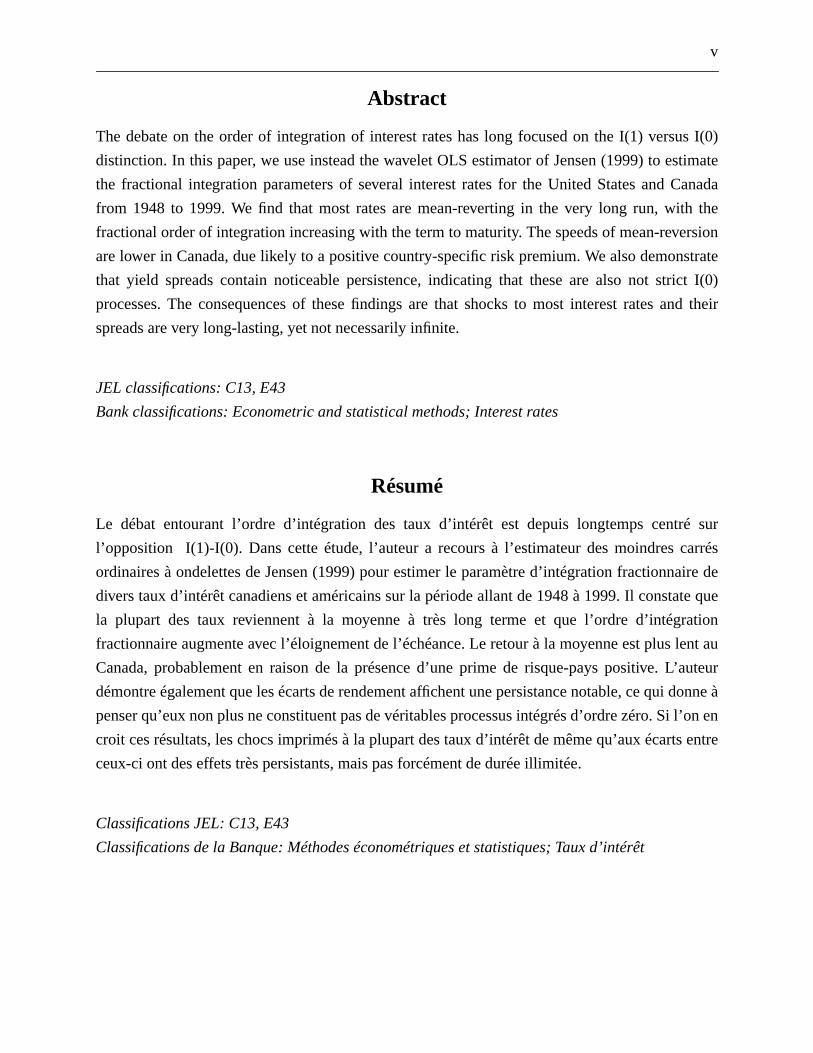
Abstract
The debate on the order of integration of interest rates has long focused on the I(1) versu
distinction. In this paper, we use instead the wavelet OLS estimator of Jensen (1999) to es
the fractional integration parameters of several interest rates for the United States and C
from 1948 to 1999. We find that most rates are mean-reverting in the very long run, with
fractional order of integration increasing with the term to maturity. The speeds of mean-reve
are lower in Canada, due likely to a positive country-specific risk premium. We also demon
that yield spreads contain noticeable persistence, indicating that these are also not stri
processes. The consequences of these findings are that shocks to most interest rates a
spreads are very long-lasting, yet not necessarily infinite.
JEL classifications: C13, E43
Bank classifications: Econometric and statistical methods; Interest rates
é sur
arrés
aire de
te que
ation
lent au
’auteur
donne à
l’on en
s entre
Résumé
Le débat entourant l’ordre d’intégration des taux d’intérêt est depuis longtemps centr
l’opposition I(1)-I(0). Dans cette étude, l’auteur a recours à l’estimateur des moindres c
ordinaires à ondelettes de Jensen (1999) pour estimer le paramètre d’intégration fractionn
divers taux d’intérêt canadiens et américains sur la période allant de 1948 à 1999. Il consta
la plupart des taux reviennent à la moyenne à très long terme et que l’ordre d’intégr
fractionnaire augmente avec l’éloignement de l’échéance. Le retour à la moyenne est plus
Canada, probablement en raison de la présence d’une prime de risque-pays positive. L
démontre également que les écarts de rendement affichent une persistance notable, ce qui
penser qu’eux non plus ne constituent pas de véritables processus intégrés d’ordre zéro. Si
croit ces résultats, les chocs imprimés à la plupart des taux d’intérêt de même qu’aux écart
ceux-ci ont des effets très persistants, mais pas forcément de durée illimitée.
Classifications JEL: C13, E43
Classifications de la Banque: Méthodes économétriques et statistiques; Taux d’intérêt

1
cs, for
ed in
ents in
ctivity.
ments
der of
r one,
these
ation
ilable,
noted
nt a
ue. In
ould
not be
nity
dom
y. In
mple,
c risk
ations
l term
st rate
terest
nomic
though
unit
ates.
1. Introduction
Interest rates play important roles in both macroeconomics and finance. In macroeconomi
example, they are crucial to the conduct of monetary policy, as policy is primarily implement
most developed countries through the setting of short-term interest rates. Interest rate movem
turn have an impact on spending and saving decisions, thereby affecting macroeconomic a
The finance literature is also prolific in models of, and uses for, interest rates, since their move
are crucial to investment and portfolio decisions.
In modern time-series econometrics, it has become standard practice to verify the or
integration of each variable entering a model. If variables are found to be integrated of orde
denoted I(1), then the focus shifts towards locating cointegrating relationships between
variables in order to exploit any long-run equilibrium properties of the data. The order of integr
of each variable is usually determined using one or more of the countless unit root tests ava
where the null of a unit root is tested against the alternative of (mean or trend) stationarity, de
I(0), or vice-versa. Dolado, Jenkinson, and Sovilla-Rivero (1990), for example, prese
comprehensive survey on unit roots.
The order of integration of nominal interest rates has long remained a contentious iss
theory, it is impossible for interest rates to follow a unit root process without drift, since this w
impose no bounds on the movements of such variables; in practice, however, they can
negative. If a drift term is included, it is also difficult to justify how interest rates can tend to infi
in the presence of a unit root. This would imply that expected inflation would also follow a ran
walk, with the consequence that its path cannot be influenced by monetary polic
macroeconomics, one would also imagine that shocks to interest rates resulting from, for exa
a currency crisis would eventually dissipate once the crisis subsides. Thus, country-specifi
premiums embedded within interest rates would have to be relatively constant, with pertub
being short-lived. Similarly, a stationary interest rate process is also a requirement of financia
structure models of the type of Cox, Ingersoll, and Ross (1985), since the short-term intere
factor has to be mean-reverting in order to make the model tractable.
In practice, however, several authors have failed to reject the unit root hypothesis for in
rates. For example, in their tests for the presence of unit roots in several key macroeco
variables, Nelson and Plosser (1982) find that the interest rate series is an I(1) process. Al
reversing most of the unit root conclusions through the introduction of structural breaks in the
root tests, Perron (1989) is unable to reverse the Nelson and Plosser conclusion for interest r
2
s, it is
thors
sense
cay of
e
ium
how
ng for
ann,
ocess
have
series
and of
of all
mory
flation
g time
their
terest
be
andard
er
ther
eter
983),
erties.
el is
Because empirical studies are unable to reject the unit root hypothesis for interest rate
quite likely that the I(0) alternative is too stringent for the unit root tests used. Instead, some au
have suggested that interest rates may in fact be fractionally integrated, or I(d), where 0 <d < 1.
Whend is estimated to lie between 0 and 0.5, the process is said to exhibit long memory in the
that the autocorrelation function (ACF) decays at a much slower rate than the exponential de
the ACF exhibited by stationary ARMA processes. In other words, the rate of interest at timt is
correlated to the rate att-k for somek > 0; this correlation diminishes, but is non-negligible, ask
increases. Whendequals 0.5 or greater but less than 1, the process will still return to its equilibr
in the long run but will also possess an infinite variance.
In previous work on fractional integration and interest rates, Backus and Zin (1993) s
that there is some evidence of long memory in the 3-month zero-coupon rate, and that allowi
long memory in the short rate improves the fitted mean and volatility yield curves. Pf
Schotman, and Tschernig (1996) also find that allowing for long memory in the short-term pr
improves the fit of term structure models.
Intuitively, interest rates may be slowly mean-reverting even if few shocks tend to
long-lasting effects. Parke (1999) introduces error-duration models that can generate
displaying long memory. The basic idea is that shocks can be of a stochastic magnitude
stochastic duration; an observed value of a variable at a point in time is essentially a sum
shocks that survive up to that point. If only a few shocks are long-lasting, then a long-me
process can ensue. In the case of nominal interest rates, significant shocks to in
expectations—such as those resulting from shifts in policy regimes—may indeed take a lon
to dissipate, and thus nominal interest rates may take a long time prior to reverting to
respective means. If a number of notable long-lasting shocks occur within a short period, in
rates may indeed behave like non-stationary processes.
If interest rates are I(d), then this may help explain why the null of a unit root cannot
rejected for such variables. For example, Diebold and Rudebusch (1991) conclude that the st
Dickey-Fuller test has low power against I(d) alternatives. As such, outright estimation of the ord
of integrationd may prove more useful than the use of low-power tests in determining whe
interest rates possess a unit root.
Several methods have been proposed to estimate the fractional integration paramd.
Among the most popular is the frequency domain method of Geweke and Porter-Hudak (1
henceforth GPH. Unfortunately, this estimator possesses no satisfactory asymptotic prop
Sowell (1990) proposes a maximum likelihood method to estimated and the ARMA(p,q)
parameters jointly; as with all maximum likelihood methods, it can perform poorly if the mod
3
the
s of
ts
s, but
ort-
errors
H
odels
) show
sis of
g
f
g the
on
risk
the
ted a
g that
ed that
r a
hange
994)
ed,
them
, and
ance
misspecified. Backus and Zin (1993) use Sowell’s estimator in their empirical work, but
divergent estimates ofd that they obtain for each ARFIMA specification reduce the usefulnes
their results.
Jensen (1999) proposes a new estimator ofd that is constructed using wavelets. Wavele
can be described most simply as functional transforms in the same spirit as Fourier transform
with properties that allow them to identify more effectively either long rhythmic behaviour or sh
run phenomena. Jensen’s wavelet ordinary least squares (WOLS) estimator ofd is derived from the
smooth decay of long-memory processes. From Jensen’s simulations, the mean squared
(MSEs) of the estimates ofd are roughly four to six times smaller than the MSEs of the GP
estimator at the sample sizes that are of interest to us in this study (sample sizesT = 256 or 512
observations). This estimator and its properties are discussed more fully below.
Once a proper estimate of the fractional order of integration is obtained, more robust m
can be constructed that exploit the properties of the data. For example, Cheung and Lai (1993
how one can utilize the information content of fractionally integrated processes in an analy
purchasing power parity. More generally, if we assume that two processesx1 andx2 are fractionally
integrated such thatx1~I(d) andx2~I(d) with 0 < d < 1, then a long-run fractional cointegratin
relationship may exist fory = f(x1,x2) ~ I(d - b), whereb < d, which may be short-run stationary i
(d - b) = 0, or follow a long-memory process if (d - b) < 1.0. If the latter, thenx1 andx2 are said to be
fractionally cointegrated, and an error-correction term would be most useful in determinin
equilibrium relationship to which the series will revert in the very long run. Our discussion
fractional cointegration is expanded in Section 4 within the context of yield spreads and
premiums.
To motivate the important implications of fractional cointegration, consider for example
debate surrounding the empirical work of Baillie and Bollerslev (1989). These authors estima
cointegrating vector for a group of seven exchange rates from industrial countries, assumin
each exchange rate was I(1). Diebold, Gardeazabal, and Yilmaz (1994) subsequently argu
the error-correction term arising from the Baillie and Bollerslev work failed to improve ove
simple martingale in an ex ante forecasting experiment, casting doubt on whether the exc
rates were cointegrated at all. Reconsidering their original findings, Baillie and Bollerslev (1
find that the error-correction term arising from their original model is not I(0) as originally believ
but I(0.89); that is, their original variables turn out to be fractionally cointegrated. This leads
to conclude that adjustments to equilibrium are likely to take several years to complete
therefore their estimated error-correction term will yield improvements in forecast perform
only several years into the future.
4
st to
r
th the
mory
rated
-term
OLS
ation
nited
ads and
ation
ourier,
n. For
osine
loped
Estimates of the fractional order of integration of interest rates should be of intere
policy-makers for at least two reasons. First, knowledge ofdwill enable them to determine whethe
shocks to interest rates are short-lived, long-lived, or infinitely lived. Second, ifd < 1, then one may
suspect that cointegrating relationships involving interest rates may not be precisely I(0), wi
consequence that adjustments to re-establish an equilibrium state may follow long-me
processes. As Baillie and Bollerslev have discovered, this implies that fractionally cointeg
relationships may yield noticeable gains in forecast accuracy only within the context of longer
forecasts.
In the next section, we motivate the intuition underlying wavelets and discuss the W
estimator more fully. In Section 3, we use the WOLS estimator to obtain the fractional integr
parameters for the zero-coupon term structure data of McCulloch and Kwon (1993) for the U
States, and standard market rates for Canada. In Section 4, we investigate whether yield spre
risk premiums are fractionally integrated. The final section concludes.
2. Methodology
2.1 Basic wavelet theory
In mathematics, it is often possible to approximate a complicated function as a linear combin
of several simple expressions. One of the better-known examples is that of spectral, or F
analysis where, by the spectral representation theorem, any covariance-stationary processxt can be
expressed as a linear combination of sine and cosine functions in the frequency domai
example, the Fourier series of any real-valued functionf(x) on the [0,1] interval is expressed as
, (1)
where the parametersak, b0, andbk, for ∀ k can be solved using least squares.
However, few economic series follow the smooth cycles suggested by sine and c
functions, thereby making Fourier analysis less appealing for economists. A recently deve
alternative to Fourier transforms arewavelet transforms, where the same functionf(x) can be
expressed in the wavelet domain in the following manner:
(2)
f x( ) b0 bk 2πkxcos ak 2πkxsin+[ ]k 1=
∞
∑+=
f x( ) c0 cjkψ 2jx k–( )
k 0=
2j 1–
∑j 0=
∞
∑+=
5
d
ex
step
sed in
y its
econd,
of this
usly
n time,
out to
(1993)
ith
with ψ(x) defined as
. (3)
The group of functions for and are orthogonal an
collectively form a basis in the space of all square-integrable functionsL2 along the [0,1] interval.
The indexj is the dilation (or scaling) index, which compresses the function , and the indk
is the transition index that shifts the function . More generally, any such basis inL2(R) is
known as a wavelet, and (3) is more commonly known as the Haar wavelet.
Several different wavelets have been proposed, which usually involve smoothing the
function (3). The Daubechies (1988) wavelet is an example of such a smooth wavelet; it is u
our applications. Our choice of the Daubechies wavelet is motivated by two factors: first, b
common usage in many applications outside economics (especially signal processing); and s
because the desirable properties of the WOLS estimator were demonstrated with the use
wavelet. Several alternative wavelets are presented in, for example, Vidakovic (1999).
As noted by Jensen (1999), the strengths of wavelets lie in their ability to simultaneo
localize a process in time and scale. They can zoom in on a process’s behaviour at a point i
which is a distinct advantage over Fourier analysis. Alternatively, wavelets can also zoom
reveal any long and smooth features of a series. The interested reader is referred to Strang
and Strichartz (1993) for more extensive expositions on wavelets.
2.2 Fractional integration and the wavelet OLS estimator
Consider the random processxt,
, (4)
whereL is the lag operator,εt is i.i.d. normal with zero mean and constant varianceσ2, andd is a
differencing parameter. Whend = 0, the processxt is simply equal toεt, soxt~N(0,σ2), or xt~I(0).
Whend= 1, however,xt follows a unit root process (without drift), implying it has a zero mean w
infinite variance.
ψ x( )
1 if 0 x 12---<≤
1 if12--- x 1<≤–
0 otherwise
=
ψ jk x( ) ψ 2jx k–( )= j 0≥ 0 k 2
j<≤
ψ x( )ψ x( )
1 L–( )dxt εt=
6
As
the
, and
erest
avelet
More generally, if we allowd to take non-integer values, the processxt is said to be
fractionally integrated, making (4) an ARFIMA process (i.e., fractionally integrated ARMA).
shown by Hosking (1981), when , the autocovariance function ofxt declines
hyperbolically to zero, makingxt a long-memory process. If ,xt has an infinite variance;
however, it will still revert to its mean (or trend) in the very long run. Table A below summarizes
different values ofd and the corresponding consequences for the mean (or trend), variance
duration of a shock.
Jensen (1999) demonstrates that, for an I(d) processxt with , use of the
autocovariance function implies that the wavelet coefficients cjk in (2) are distributed as
. If R(j) denotes the wavelet coefficient’s variance at scalej, then after taking
logarithms, an estimate ofd can be obtained from
. (5)
Thus, the wavelet transform is applied to the autocovariance function of a particular int
rate, not to the interest rate itself. The wavelets are used only in the estimation of thed consistent
with the observed autocovariance function. Furthermore, because of the form of the w
expansion (2), it should be noted that the number of observations for the underlying processxt must
be a factor of 2.
Table A: Summary of fractional integration parameter values
d Mean (or trend) and variance Shock duration
Short-run mean-reversionFinite variance
Short-lived
Long-run mean-reversionFinite Variance
Long-lived
Long-run mean-reversionInfinite variance
Long-lived
No mean-reversionInfinite variance
Infinite
No mean-reversionInfinite variance
Infinite; effect increases astime moves forward
0 d 12---< <
12--- d 1<≤
d 12---<
N 0 σ22
2jd–,( )
R j( )ln σ2 d 22j
ln–ln=
d 0=
0 d 0.5< <
0.5 d 1<≤
d 1=
d 1>
7
ple size
have
th
tained
and
ns are
ple. To
fferent
order of
st two
tes on
g that
ack to
e term
he rates
ned by
f the
ever,
after
ty is
rences
ration
ugh to
ted
o not use
t cause
ults are
3. Estimates ofd for interest rate levels
We consider several nominal interest rates for the United States and Canada. Given the sam
restrictions for the implementation of the estimation, we use monthly data such that we
common sample sizes ofT = 28 = 256 andT = 29 = 512 observations. We use 1-, 3-, 6-, and 9-mon
T-bill rates, and 1-, 3-, 5-, and 10-year zero-coupon bond rates from 1948:7 to 1991:2, all ob
from McCulloch and Kwon (1993) for the United States. CANSIM data for commercial paper
government bond rates are used for Canada from 1956:11 to 1999:6. The computatio
performed using the Matlab toolboxWavekitof Ojanen (1998).
3.1 United States
In Table 1 we present the estimates of the fractional integration parameters over the full sam
verify the robustness of our results, we consider the unsmooth Haar wavelet, and three di
degrees of smoothing for the Daubechies wavelet, where the smoothness increases with the
the wavelet. Three important findings emerge. First, all estimated parameters are at lea
standard errors above 0.5, indicating that all rates have an infinite variance. Second, all ra
securities with maturities of one year or less are at least two standard errors below 1.0, implyin
they are not strict unit root processes. The implication is that they have a tendency to revert b
their means in the very long run. Finally, the fractional integration parameters increase as th
to maturity increases. We therefore find that the longest rates, the 5- and 10-year rates, are t
that display properties that most closely resemble unit processes. This evidence is strengthe
examining the autocorrelation functions plotted in Figure 1. We see that the decay o
autocorrelations of the 1-month rate is more pronounced than it is for the 10-year rate. How
both series display very slow decay overall, with the autocorrelations remaining positive even
five years.
The finding of increasing “non-stationariness” with increases in the term to maturi
probably one of the more interesting results. Since we are using zero-coupon rates, any diffe
we uncover are likely due to the effects of term premia. Thus, because the order of integ
increases with the term, we suspect that term premia are non-constant and fluctuate eno
induce the longest rates to follow unit root processes.
In Table 2, we trim our sample to 28 = 256 observations to examine whether the estima
parameters change in notable manners. This exercise is useful because researchers often d
data from the 1940s and 1950s, since the thin bond markets in existence at that time did no
interest rates to fluctuate much in response to market conditions, as they do today. The res
8
ger, as
veral
s may
rates
in two
g the
o as a
both
years
here is
mple,
less non-
s from
ration
esults,
two
th the
to their
yield
e two
rates on
se that
s. The
asing
years
r to be
short
now less straightforward. We find that the standard errors of the estimates are noticeably lar
we would expect given the smaller sample size. The implication is that there are now se
estimated parameters within two standard errors of 0.5, indicating that some interest rate
exhibit properties of long-run mean-reversion with finite variance. This feature emerges for all
using the Daubechies wavelets. The second result is that the longer-term rates are still with
standard errors of the unit root scenario. However, the significant uncertainty surroundin
estimates prevents us from making any firm conclusions other than we can still exclude zer
possible order of integration.
Examining the autocorrelation functions for this sample (Figure 2), we now find that
short- and long-term rates decay more quickly, with autocorrelations reaching zero after 3.5
for the 1-month rate and 4.5 years for the 10-year rate. Based on this evidence, we find that t
significant improvement in the rate of mean-reversions for all interest rates over the shorter sa
and this is reflected in the estimated parameters. We can also state that the shorter rates are
stationary than the longer rates, again due presumably to the effects of term premia.
3.2 Canada
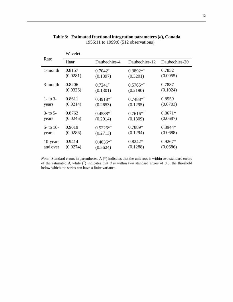
In Table 3, we present the fractional integration parameters for the Canadian interest rate
1956 to 1999. Using the Haar and Daubechies-20 wavelets, we find that the order of integ
tends to rise as the term to maturity increases from one month to ten years. As with the U.S. r
we find that the long-term rate is most likely to follow a unit root process. Results using the
other wavelets are largely inconclusive, given the large standard errors associated wi
estimates. The autocorrelation functions in Figure 3 demonstrate that short-term rates revert
means more quickly, consistent with lower orders of integration.
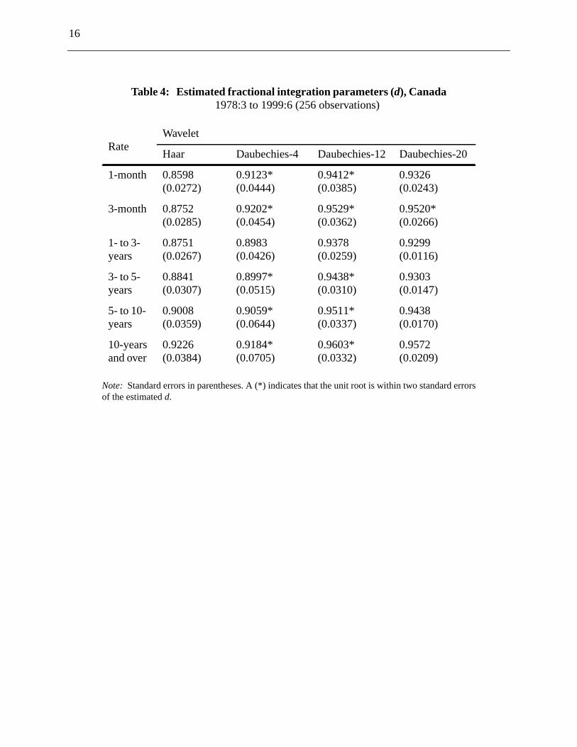
When focusing on the second half of the sample (Table 4), we find that all wavelets
very similar estimates. Unlike our previous results, we find that the orders of integration on th
shortest rates are somewhat higher than for the longer-term rates. Recalling that these are
commercial paper, which carry a greater default risk than government bonds, we can surmi
the relatively higher estimates on the short rates are due to the changing effects of such risk
fractional integration parameters for bond rates from one year onwards display a similar incre
pattern that we have explained previously as likely due to varying term premiums.
The orders of integration on these variables estimated for data covering the last 21
suggest that all rates follow near unit root processes, clearly are not I(0), and would appea
long-run mean-reverting. Figure 4 suggests that after five years the autocorrelations of both
9
longer
ns that
s and
in the
essed
risk-
s. The
ch, we
sing
ers of
real
ion
f
on
he
and long rates remain positive, thereby providing visual evidence that Canadian rates have
memory than their U.S. counterparts.
4. Estimates ofd for spreads and real rates
The purpose of this section is to estimate the orders of integration of standard transformatio
are often applied to nominal interest rates. We consider both long-short yield spread
adjustments for inflation.
We can decompose the long (10-year) and short (3-month) nominal interest rates
following manner:
(6)
(7)
wherer is the real rate,πe is expected inflation,rpcanis a country-specific risk-premium (which is
assumed to equal zero for the United States and to be greater than zero for Canada), andterm is a
positive term risk premium. Subtracting (7) from (6), we find that the yield spread can be expr
in two different manners:
, (8)
or
. (9)
Equation (8) states that the nominal yield spread equals the difference between
premium-adjusted real rates, while (9) states that it equals the inflation-adjusted nominal rate
real rates, country-specific risk premium, and the term premium are all unobservable. As su
cannot formally estimate the orders of integration of the components in (8). However, by u
actual inflation as a proxy for expected inflation, we can at least estimate the fractional ord
integration of all terms entering (9). This allows us to determine whether our proxies for the
rates follow long-memory processes.
Recall that two I(d) variables are said to be fractionally cointegrated if a linear combinat
of these variables yields an I(d-b) series, whered-b< d. If the two variables are of different orders o
integration, sayd1 andd2, they are fractionally cointegrated if the resulting linear combinati
yields an I(d-b) series, whered = min(d1,d2). We are therefore interested in knowing whether t
i10 r10 πe rpcan term+ + +=
i3 r3 πe rpcan+ +=
i10 i3–( ) r10 rpcan term+ +( ) r3 rpcan+( )–=
i10 i3–( ) i10 πe–( ) i3 πe
–( )–=
10
both
l rates
t. Louis
inal
of the
lent of
er of
ory
pected
f the
yield
ates to
s that
timates
rate. As
imple
der of
what
sistent
in
rslev
only at
mory
arterly
fractional order of integration of the yield spread is lower than the orders of integration of
nominal and real rates, which is evidence of fractional cointegration between the rates.
4.1 United States
In Table 5, we present the orders of integration of (expected) inflation, nominal rates, nomina
less expected inflation, and the yield spread. The rates used here are obtained from the S
Fed, and expected inflation is the year-over-year growth of total CPI. Beginning with the nom
rates, we find that the orders of integration are all above 0.86, while the order of integration
spread is 0.66 or less. This implies that the simple difference of the rates, which is the equiva
a [1, -1] cointegration vector, yields a process of lower order of integration. However, the ord
integration of the yield spread is noticeably above 0.0, implying that it follows a long-mem
process.
In the same table, we also present the orders of integration of the nominal rates less ex
inflation, as denoted in (9). For each individual wavelet, we find that the orders of integration o
“expected-inflation-adjusted” rates are again greater than the order of integration of the
spread. For example, for the Daubechies-12 wavelet, we find the order of the long and short r
be 0.8830 and 0.7348 respectively, both larger than the spread order of 0.6625. This implie
both of these series are also fractionally cointegrated. That is, the difference between the es
of long and shortreal rates yields a long-term relationship that is mean-reverting.
4.2 Canada
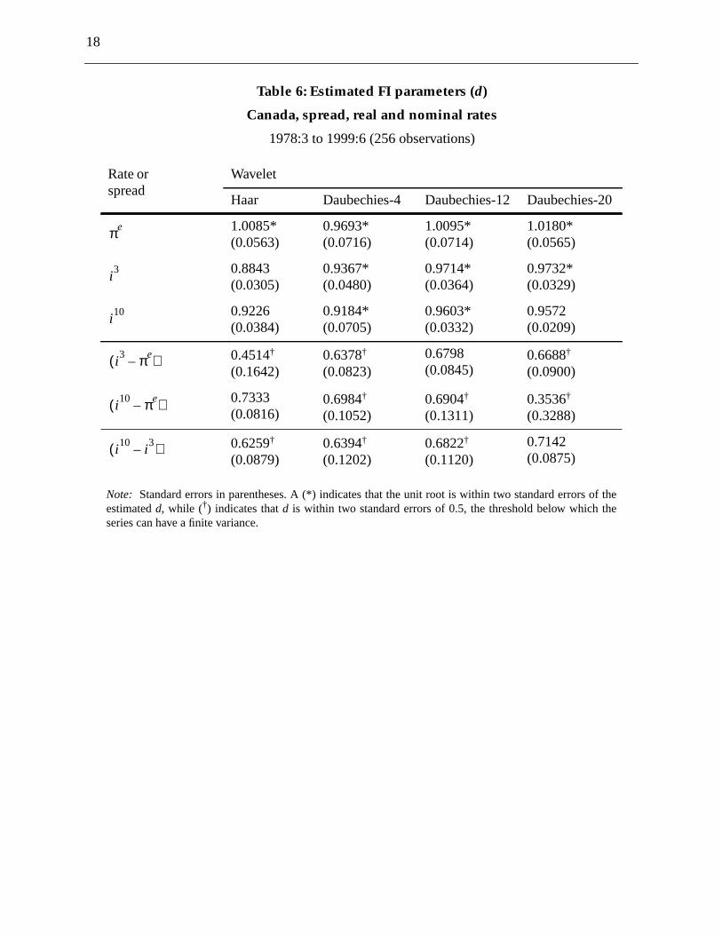
We present the Canadian results in Table 6. The short rate used here is a 90-day treasury bill
with the United States, we find that the nominal rates are fractionally cointegrated, since the s
yield spread has an order of integration lower than the individual nominal rates. In fact, the or
integration is around 0.65, a similar order as for the United States.
The finding that the long-short yield spread is a long-memory process is some
surprising, since it has always been believed to be a stationary I(0) process. However, it is con
with empirical work that has found it to be a good indicator of economic activity, peaking
explanatory power at the 4- to 6-quarter forecast horizon. As explained by Baillie and Bolle
(1994), long-memory error-correction terms should possess adequate forecasting power
longer horizons. The spread is, in fact, a [1,-1] cointegration vector; therefore, if it is a long-me
process, it should be most useful at longer horizons. Short-memory variables, such as the qu
growth rate of money, should be superior short-run predictors.
11
t the
yield
tion-
has an
that a
risk-
t with
n than
more
ted by a
recent
der of
se to
1948
most
e with
ricting
rity is
s, may
tates
ersion
mory
rates,
es that
above,
al risk
rparts
Returning to Table 6, subtracting expected inflation from the nominal rates, we find tha
orders of integration of either the short or long rate are below the order of integration of the
spread. For example, with the Daubechies-12 wavelet, the order of integration of the infla
adjusted short rate is 0.6798; for the long rate, it is 0.6904. The simple yield spread, however,
order of integration of 0.6822. This implies that these rates are either not cointegrated, or
[1, -1] cointegration vector is not appropriate. We may conjecture that the country-specific
premium terms in (8) are the cause of the additional non-stationarity. This would be consisten
our earlier observation that nominal Canadian rates have larger fractional orders of integratio
their U.S. counterparts. The economic implication is that a world interest rate shock will be
rapidly absorbed by U.S. rates than Canadian rates, since the Canadian rates are also affec
non-stationary risk premium.
5. Conclusion
This paper estimates the fractional integration parameters for several interest rates using a
estimator with desirable properties. The purpose is to contribute to the debate on the or
integration of nominal interest rates. The estimated orders of integration may be of u
macroeconomic and financial modellers who seek more robust results.
Our findings differ somewhat over U.S. and Canadian rates. For the United States from
to 1991, all short-term interest rates are long-run mean-reverting, while longer-term rates are
likely to follow unit root processes, as the estimated fractional integration parameters increas
the term to maturity. Non-constant term premia may be the cause of this last result. When rest
our attention to the latter half of the sample, we find that the evidence in favour of non-stationa
diminished. This leaves open the possibility that some rates, especially at the shorter horizon
be following stationary long-memory processes.
Overall, we conclude that the unit root hypothesis is unduly harsh for the United S
except for the longer-term interest rates. Furthermore, the assumption of short-run mean-rev
is also strongly rejected by the data. The hypothesis that nominal interest rates follow long-me
processes seems the most plausible.
Canadian rates also exhibit strong persistence over the full sample. Unlike the U.S.
however, this persistence remains even over the second half of the sample. This indicat
shocks to interest rates take longer to dissipate in Canada than the United States. As we noted
long-term bonds may be more non-stationary than short-term bonds due to the addition
captured in the term premia. Canadian bonds are usually riskier than their American counte
12
ent of
t, the
more
sed in
ords,
ake a
iven
ay be
hort-
due to, for example, political uncertainty and exchange rate movements. This additional elem
risk may be reflected in the larger order of integration of Canadian bonds in the last 20 years.
For the applied researcher, the following conclusions emerge from our findings. Firs
rate of mean-reversion decreases with the term to maturity, with longer-term rates reverting
slowly, if at all, to their means than short-term rates. Second, if these interest rates are u
cointegration analysis, then the underlying vectors may not be strict I(0) processes. In other w
if the cointegrating relationship is fractionally integrated, then adjustments to shocks may t
long time to be finalized. Finally, the fractional order of integration may indicate whether a g
variable would be most adequate as a short-run or long-run indicator. A I(0.60) variable m
preferable for long-run forecasts, while an I(0) variable would be most appropriate for the s
run.
13
Table 1: Estimated fractional integration parameters (d), United States1948:7 to 1991:2 (512 observations)
Note: Standard errors in parentheses. A (*) indicates that the unit root is within two standard errorsof the estimatedd.
RateWavelet
Haar Daubechies-4 Daubechies-12 Daubechies-20
1-month 0.8127(0.0334)
0.8479(0.0346)
0.8608(0.0318)
0.8550(0.0324)
3-month 0.8444(0.0329)
0.8806(0.0387)
0.8891(0.0318)
0.8866(0.0331)
6-month 0.8533(0.0325)
0.8909(0.0402)
0.8950(0.0285)
0.8928(0.0281)
9-month 0.8570(0.0324)
0.8930(0.0387)
0.8976(0.0258)
0.8930(0.0246)
1-year 0.8701(0.0319)
0.9010(0.0365)
0.9089(0.0231)
0.9007(0.0214)
3-year 0.9267(0.0336)
0.9414*(0.0337)
0.9547(0.0185)
0.9424(0.0152)
5-year 0.9550*(0.0395)
0.9640*(0.0346)
0.9791*(0.0202)
0.9672*(0.0185)
10-year 0.9885*(0.0462)
0.9951*(0.0327)
1.0098*(0.0215)
0.9948*(0.0228)
14
Table 2: Estimated FI parameters (d), United States1969:11 to 1991:2 (256 observations)
Note: Standard errors in parentheses. A (*) indicates that the unit root is within two standard errorsof the estimatedd, while (†) indicates thatd is within two standard errors of 0.5, the thresholdbelow which the series can have a finite variance.
RateWavelet
Haar Daubechies-4 Daubechies-12 Daubechies-20
1-month 0.7168(0.0491)
0.7075†
(0.1066)0.6756†
(0.1335)0.4706†
(0.2474)
3-month 0.7604(0.0521)
0.7491(0.1151)
0.7007†
(0.1425)0.5667*†
(0.2186)
6-month 0.7654(0.0545)
0.7681(0.1098)
0.7147†
(0.1325)0.5244*†
(0.2404)
9-month 0.7681(0.0524)
0.7648(0.1103)
0.7086†
(0.1338)0.5527†
(0.2205)
1-year 0.7845(0.0492)
0.7609(0.1167)
0.7025†
(0.1441)0.6176†
(0.1880)
3-year 0.8464(0.0415)
0.7118*†
(0.1713)0.5351*†
(0.2692)
0.7800*(0.1181)
5-year 0.8737(0.0480)
0.6820*†
(0.2087)0.5456*†
(0.2854)
0.8389*(0.1059)
10-year 0.9024*(0.0558)
0.6327*†
(0.2630)0.7217*†
(0.2115)
0.8998*(0.0974)
15
Table 3: Estimated fractional integration parameters (d), Canada1956:11 to 1999:6 (512 observations)
Note: Standard errors in parentheses. A (*) indicates that the unit root is within two standard errorsof the estimatedd, while (†) indicates thatd is within two standard errors of 0.5, the thresholdbelow which the series can have a finite variance.
RateWavelet
Haar Daubechies-4 Daubechies-12 Daubechies-20
1-month 0.8157(0.0281)
0.7042†
(0.1397)0.3892*†
(0.3201)0.7852(0.0955)
3-month 0.8206(0.0326)
0.7241†
(0.1301)0.5765*†
(0.2190)0.7887(0.1024)
1- to 3-years
0.8611(0.0214)
0.4918*†
(0.2653)0.7488*†
(0.1295)0.8559(0.0703)
3- to 5-years
0.8762(0.0246)
0.4588*†
(0.2914)0.7616*†
(0.1309)0.8671*(0.0687)
5- to 10-years
0.9019(0.0286)
0.5226*†
(0.2713)0.7889*(0.1294)
0.8944*(0.0688)
10-yearsand over
0.9414(0.0274)
0.4036*†
(0.3624)0.8242*(0.1288)
0.9267*(0.0686)
16
Table 4: Estimated fractional integration parameters (d), Canada1978:3 to 1999:6 (256 observations)
Note: Standard errors in parentheses. A (*) indicates that the unit root is within two standard errorsof the estimatedd.
RateWavelet
Haar Daubechies-4 Daubechies-12 Daubechies-20
1-month 0.8598(0.0272)
0.9123*(0.0444)
0.9412*(0.0385)
0.9326(0.0243)
3-month 0.8752(0.0285)
0.9202*(0.0454)
0.9529*(0.0362)
0.9520*(0.0266)
1- to 3-years
0.8751(0.0267)
0.8983(0.0426)
0.9378(0.0259)
0.9299(0.0116)
3- to 5-years
0.8841(0.0307)
0.8997*(0.0515)
0.9438*(0.0310)
0.9303(0.0147)
5- to 10-years
0.9008(0.0359)
0.9059*(0.0644)
0.9511*(0.0337)
0.9438(0.0170)
10-yearsand over
0.9226(0.0384)
0.9184*(0.0705)
0.9603*(0.0332)
0.9572(0.0209)
17
e
Table 5: Estimated FI parameters (d)
United States spread, real and nominal rates
1978:3 to 1999:6 (256 observations)
Note: Standard errors in parentheses. A (*) indicates that the unit root is within two standard errors of thestimatedd, while (†) indicates thatd is within two standard errors of 0.5, the threshold below which theseries can have a finite variance.
Rate orSpread
Wavelet
Haar Daubechies-4 Daubechies-12 Daubechies-20
1.0142*(0.0682)
0.9282*(0.1567)
0.9421*(0.1608)
1.0131*(0.1135)
0.8645(0.0410)
0.8814*(0.0634)
0.9394*(0.0592)
0.9423*(0.0414)
0.9226*(0.0611)
0.9502*(0.0871)
1.0099*(0.0542)
1.0122*(0.0275)
0.6402†
(0.1112)0.7104(0.0809)
0.7348(0.0966)
0.7530(0.0716)
0.7560*†
(0.1378)0.6807*†
(0.2555)0.8830*(0.1234)
0.9383*(0.0906)
0.3457†
(0.2433)0.6549†
(0.0969)0.6625†
(0.1054)0.5948†
(0.1536)
πe
i3
i10
i3 πe–( )
i10 πe–( )
i10 i3–( )
18
e
Table 6: Estimated FI parameters (d)
Canada, spread, real and nominal rates
1978:3 to 1999:6 (256 observations)
Note: Standard errors in parentheses. A (*) indicates that the unit root is within two standard errors of thestimatedd, while (†) indicates thatd is within two standard errors of 0.5, the threshold below which theseries can have a finite variance.
Rate orspread
Wavelet
Haar Daubechies-4 Daubechies-12 Daubechies-20
1.0085*(0.0563)
0.9693*(0.0716)
1.0095*(0.0714)
1.0180*(0.0565)
0.8843(0.0305)
0.9367*(0.0480)
0.9714*(0.0364)
0.9732*(0.0329)
0.9226(0.0384)
0.9184*(0.0705)
0.9603*(0.0332)
0.9572(0.0209)
0.4514†
(0.1642)0.6378†
(0.0823)0.6798(0.0845)
0.6688†
(0.0900)
0.7333(0.0816)
0.6984†
(0.1052)0.6904†
(0.1311)0.3536†
(0.3288)
0.6259†
(0.0879)0.6394†
(0.1202)0.6822†
(0.1120)0.7142(0.0875)
πe
i3
i10
i3 πe–( )
i10 πe–( )
i10 i3–( )
19
Figure 1: Autocorrelation functions, U.S. 1-month and 10-year rates, 1948:7 to 1991:2
Figure 2: Autocorrelation functions, U.S. 1-month and 10-year rates, 1969:11 to 1991:2
0 10 20 30 40 50 60
0.00
0.25
0.50
0.75
1.001-Month
10-Year
0 10 20 30 40 50 60
-0.2
0.0
0.2
0.4
0.6
0.8
1.01-Month
10-Year
20
Figure 3: Autocorrelation functions, Cdn. 1-month and 10-year rates, 1956:11 to 1999:6
Figure 4: Autocorrelation functions, Cdn. 1-month and 10-year rates, 1978:3 to 1999:6
0 10 20 30 40 50 60
0.00
0.25
0.50
0.75
1.001-Month
10-Year
0 10 20 30 40 50 60
0.1
0.2
0.3
0.4
0.5
0.6
0.7
0.8
0.9
1.01-Month
10-Year
21
erm
ates.”
wer
tes.”
Rate
ional
ime
ator of
tate
eries:
s,
References
Backus, D. K. and S. E. Zin. 1993. “Long-Memory Inflation Uncertainty: Evidence from the TStructure of Interest Rates.”Journal of Money, Credit and Banking25: 681–700.
Baillie, R. T. and T. Bollerslev. 1989. “Common Stochastic Trends in a System of Exchange RJournal of Finance44: 167–181.
———. 1994. “Cointegration, Fractional Cointegration, and Exchange Rate Dynamics.”Journal ofFinance49: 737–745.
Cheung, Y.-W. and K. S. Lai. 1993. “A Fractional Cointegration Analysis of Purchasing PoParity.”Journal of Business and Economic Statistics11: 103–112.
Cox, J., J. Ingersoll, and S. Ross. 1985. “A Theory of the Term Structure of Interest RaEconometrica53: 385–408.
Daubechies, I. 1988. “Orthonormal Bases of Compactly Supported Wavelets.”Communications onPure and Applied Mathematics41: 909–996.
Diebold, F. X., J. Gardeazabal, and K. Yilmaz. 1994. “On Cointegration and ExchangeDynamics.”Journal of Finance49: 727–735.
Diebold, F. X. and G. D. Rudebusch. 1991. “On the Power of Dickey Fuller Test Against FractAlternatives.”Economics Letters35: 155–160.
Dolado, J. J., T. Jenkinson, and S. Sovilla-Rivero. 1990. “Cointegration and Unit Roots.”Journal ofEconomic Surveys4: 249–273.
Geweke, J. and S. Porter-Hudak. 1983. “The Estimation and Application of Long Memory TSeries Models.”Journal of Time Series Analysis4: 221–238.
Hosking, J. R. 1981. “Fractional Differencing.”Biometrika68: 165–176.
Jensen, M. J. 1999. “Using Wavelets to Obtain a Consistent Ordinary Least Squares Estimthe Long-memory Parameter.”Journal of Forecasting18: 17–32.
McCulloch, J. H. and H.-C. Kwon. 1993. “U.S. Term Structure Data, 1947-1991.” Ohio SUniversity Working Paper No. 93-6.
Nelson, C. R. and C. I. Plosser. 1982. “Trends and Random Walks in Macroeconomic Time SSome Evidence and Implications.”Journal of Monetary Economics10: 139–162.
Ojanen, H. 1998. “WAVEKIT: A Wavelet Toolbox for Matlab.” Department of MathematicRutgers University.
Parke, W. R. 1999. “What is Fractional Integration?”The Review of Economics and Statistics81:632–638.
22
sis.”
s and
Perron, P. 1989. “The Great Crash, the Oil Price Shock and the Unit Root HypotheEconometrica57: 1361–1401.
Pfann, G. A., P. C. Schotman, and R. Tschernig. 1996. “Nonlinear Interest Rate DynamicImplications for the Term Structure.”Journal of Econometrics74: 149–176.
Sowell, F. 1990. “The Fractional Unit Root Distribution.”Econometrica58: 495–505.
Strang, G. 1993. “Wavelet Transforms Versus Fourier Transforms.”Bulletin of the AmericanMathematical Society28: 288–305.
Strichartz, R. S. 1993. “How to Make Wavelets.”American Mathematical Monthly100: 539–556.
Vidakovic, B. 1999.Statistical Modeling by Wavelets. New York: John Wiley and Sons.
Bank of Canada Working PapersDocuments de travail de la Banque du Canada
Working papers are generally published in the language of the author, with an abstract in both official lan-guages.Les documents de travail sont publiés généralement dans la langue utilisée par les auteurs; ils sontcependant précédés d’un résumé bilingue.
20002000-4 Quelques résultats empiriques relatifs à l’évolution du taux de change
Canada/États-Unis R. Djoudad and D. Tessier
2000-3 Long-Term Determinants of the Personal Savings Rate: Literature Reviewand Some Empirical Results for Canada G. Bérubé and D. Côté
2000-2 GAUSSTM Programs for the Estimation of State-Space Models withARCH Errors: A User’s Guide M. Kichian
2000-1 The Employment Costs of Downward Nominal-Wage Rigidity J. Farès and S. Hogan
199999-20 The Expectations Hypothesis for the Longer End of the Term Structure:
Some Evidence for Canada R. Lange
99-19 Pricing Interest Rate Derivatives in a Non-ParametricTwo-Factor Term-Structure Model J. Knight, F. Li, and M. Yuan
99-18 Estimating One-Factor Models of Short-Term Interest Rates D. Mc Manus and D. Watt
99-17 Canada’s Exchange Rate Regime and North American Econo-mic Integration: The Role of Risk-Sharing Mechanisms Z. Antia, R. Djoudad, and P. St-Amant
99-16 Optimal Currency Areas: A Review of the Recent Literature R. Lafrance and P. St-Amant
99-15 The Information Content of Interest Rate Futures Options D. Mc Manus
99-14 The U.S. Capacity Utilization Rate: A New Estimation Approach R. Lalonde
99-13 Indicator Models of Core Inflation for Canada R. Dion
99-12 Why Canada Needs a Flexible Exchange Rate J. Murray
99-11 Liquidity of the Government of Canada Securities Market: Stylized Factsand Some Market Microstructure Comparisons to the United States T. Gravelle
99-10 Real Effects of Collapsing Exchange Rate Regimes:An Application to Mexico P. Osakwe and L. Schembri
99-9 Measuring Potential Output within a State-Space Framework M. Kichian
99-8 Monetary Rules When Economic Behaviour Changes R. Amano, D. Coletti, and T. Macklem
99-7 The Exchange Rate Regime and Canada’s Monetary Order D. Laidler
99-6 Uncovering Inflation Expectations and Risk Premiumsfrom Internationally Integrated Financial Markets B.S.C. Fung, S. Mitnick, and E. Remolona
Copies and a complete list of working papers are available from:Pour obtenir des exemplaires et une liste complète des documents de travail, prière de s’adresser à:
Publications Distribution, Bank of Canada Diffusion des publications, Banque du Canada234 Wellington Street Ottawa, Ontario K1A 0G9 234, rue Wellington, Ottawa (Ontario) K1A 0G9
E-mail / Adresse électronique: [email protected]: http://www.bank-banque-canada.ca/