1

Wireless Sensor Network Localization TechniquesGuoqiang Mao, Barıs Fidan and Brian D.O. Anderson

Abstract— Wireless sensor network localization is an importantarea that attracted significant research interest. This interest isexpected to grow further with the proliferation of wireless sensornetwork applications. This paper provides an overview of themeasurement techniques in sensor network localization and theone-hop localization algorithms based on these measurements.A detailed investigation on multihop connectivity-based anddistance-based localization algorithms are presented. A list ofopen research problems in the area of distance-based sensornetwork localization is provided with discussion on possibleapproaches to them.

Index Terms— wireless sensor networks, localization, AOA,RSS, TDOA.

I. INTRODUCTION

W IRELESS sensor networks (WSNs) are a significanttechnology attracting considerable research interest.

Recent advances in wireless communications and electronicshave enabled the development of low-cost, low-power andmulti-functional sensors that are small in size and commu-nicate in short distances. Cheap, smart sensors, networkedthrough wireless links and deployed in large numbers, provideunprecedented opportunities for monitoring and controllinghomes, cities, and the environment. In addition, networkedsensors have a broad spectrum of applications in the de-fence area, generating new capabilities for reconnaissance andsurveillance as well as other tactical applications [1].

Self-localization capability is a highly desirable characteris-tic of wireless sensor networks. In environmental monitoringapplications such as bush fire surveillance, water qualitymonitoring and precision agriculture, the measurement dataare meaningless without knowing the location from wherethe data are obtained. Moreover, location estimation mayenable a myriad of applications such as inventory management,intrusion detection, road traffic monitoring, health monitoring,reconnaissance and surveillance.

Sensor network localization algorithms estimate the loca-tions of sensors with initially unknown location informationby using knowledge of the absolute positions of a few sensorsand inter-sensor measurements such as distance and bearingmeasurements. Sensors with known location information arecalled anchors and their locations can be obtained by usinga global positioning system (GPS), or by installing anchorsat points with known coordinates. In applications requiringa global coordinate system, these anchors will determine thelocation of the sensor network in the global coordinate system.

G. Mao is with the University of Sydney and National ICT Australia,Sydney. B. Fidan and B. D. O. Anderson are with the Australian NationalUniversity and National ICT Australia. National ICT Australia is fundedby the Australian Governments Department of Communications, InformationTechnology and the Arts and the Australian Research Council throughthe Backing Australias Ability initiative and the ICT Centre of ExcellenceProgram.

In applications where a local coordinate system suffices (e.g.,smart homes), these anchors define the local coordinate systemto which all other sensors are referred. Because of constraintson the cost and size of sensors, energy consumption, imple-mentation environment (e.g., GPS is not accessible in some en-vironments) and the deployment of sensors (e.g., sensor nodesmay be randomly scattered in the region), most sensors do notknow their locations. These sensors with unknown locationinformation are called non-anchor nodes and their coordinateswill be estimated by the sensor network localization algorithm.

In this paper, we provide an overview of techniques thatcan be used for WSN localization. Review of wireless networklocalization techniques can be found in [2], [3], [4]. The focusof these references is on localization techniques in cellular net-work and wireless local area network (WLAN) environmentsand on the signal processing aspect of localization techniques.Sensor networks vary significantly from traditional cellularnetworks and WLAN, in that sensor nodes are assumed tobe small, inexpensive, cooperative and deployed in largequantity. These features of sensor networks present uniquechallenges and opportunities for WSN localization. Patwariet al. described some general signal processing tools that areuseful in cooperative WSN localization algorithms [5] with afocus on computing the Cramer-Rao bounds for localizationusing a variety of different types of measurements [5]. Ourreview in contrast focuses on the measurement techniquesand localization algorithms in WSNs. While many techniquescovered in this paper can be applied in both 2-dimension (<2)and 3-dimension (<3), we choose to focus on 2D localizationproblems for ease of explanation.

The rest of the paper is organized as follows. In Section II,measurement techniques in WSN localization are discussed;these include angle-of-arrival (AOA) measurements, distancerelated measurements and RSS profiling techniques. Distancerelated measurements are further classified into one-way prop-agation time and roundtrip propagation time measurements,the lighthouse approach to distance measurements, receivedsignal strength (RSS)-based distance measurements and time-difference-of-arrival (TDOA) measurements. In Section III,one-hop localization techniques based on these measurementsare discussed. Section IV discusses nonline-of-sight error mit-igation techniques in WSN localization. Section V and SectionVI focus on multihop localization techniques, in particularconnectivity-based and distance-based multihop localizationtechniques. Section VII discusses open research problems indistance-based localization. Finally a summary is provided inSection VIII.

II. MEASUREMENT TECHNIQUES

Measurement techniques in WSN localization can bebroadly classified into three categories: AOA measurements,

2

distance related measurements and RSS profiling techniques.

A. Angle-of-arrival measurements

The angle-of-arrival measurement techniques can be furtherdivided into two subclasses: those making use of the receiverantenna’s amplitude response and those making use of thereceiver antenna’s phase response.

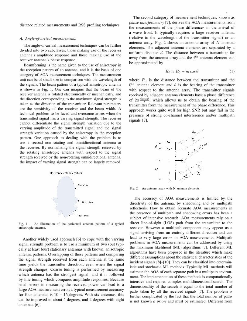
Beamforming is the name given to the use of anisotropy inthe reception pattern of an antenna, and it is the basis of onecategory of AOA measurement techniques. The measurementunit can be of small size in comparison with the wavelength ofthe signals. The beam pattern of a typical anisotropic antennais shown in Fig. 1. One can imagine that the beam of thereceiver antenna is rotated electronically or mechanically, andthe direction corresponding to the maximum signal strength istaken as the direction of the transmitter. Relevant parametersare the sensitivity of the receiver and the beam width. Atechnical problem to be faced and overcome arises when thetransmitted signal has a varying signal strength. The receivercannot differentiate the signal strength variation due to thevarying amplitude of the transmitted signal and the signalstrength variation caused by the anisotropy in the receptionpattern. One approach to dealing with the problem is touse a second non-rotating and omnidirectional antenna atthe receiver. By normalizing the signal strength received bythe rotating anisotropic antenna with respect to the signalstrength received by the non-rotating omnidirectional antenna,the impact of varying signal strength can be largely removed.

Fig. 1. An illustration of the horizontal antenna pattern of a typicalanisotropic antenna.

Another widely used approach [6] to cope with the varyingsignal strength problem is to use a minimum of two (but typi-cally at least four) stationary antennas with known, anisotropicantenna patterns. Overlapping of these patterns and comparingthe signal strength received from each antenna at the sametime yields the transmitter direction, even when the signalstrength changes. Coarse tuning is performed by measuringwhich antenna has the strongest signal, and it is followedby fine tuning which compares amplitude responses. Becausesmall errors in measuring the received power can lead to alarge AOA measurement error, a typical measurement accuracyfor four antennas is 10 − 15 degrees. With six antennas, thiscan be improved to about 5 degrees, and 2 degrees with eightantennas [6].

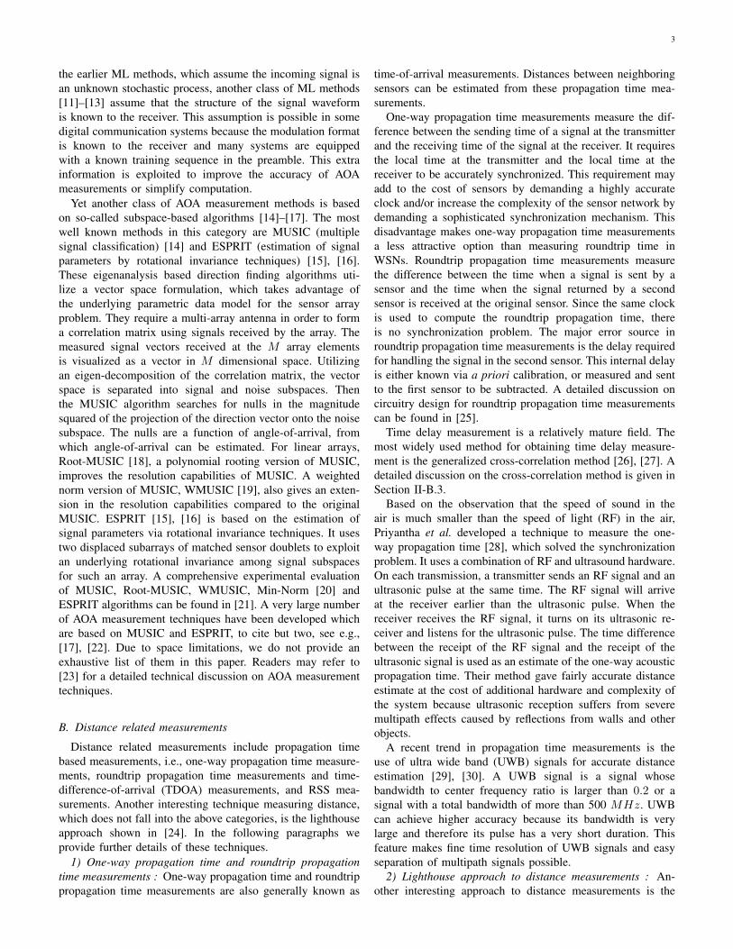
The second category of measurement techniques, known asphase interferometry [7], derives the AOA measurements fromthe measurements of the phase differences in the arrival ofa wave front. It typically requires a large receiver antenna(relative to the wavelength of the transmitter signal) or anantenna array. Fig. 2 shows an antenna array of N antennaelements. The adjacent antenna elements are separated by auniform distance d. The distance between a transmitter faraway from the antenna array and the ith antenna element canbe approximated by

Ri ≈ R0 − id cos θ (1)

where R0 is the distance between the transmitter and the0th antenna element and θ is the bearing of the transmitterwith respect to the antenna array. The transmitter signalsreceived by adjacent antenna elements have a phase differenceof 2π d cos θ

λ , which allows us to obtain the bearing of thetransmitter from the measurement of the phase difference. Thisapproach works quite well for high SNR but may fail in thepresence of strong co-channel interference and/or multipathsignals [7].

Fig. 2. An antenna array with N antenna elements.

The accuracy of AOA measurements is limited by thedirectivity of the antenna, by shadowing and by multipathreflections. How to obtain accurate AOA measurements inthe presence of multipath and shadowing errors has been asubject of intensive research. AOA measurements rely on adirect line-of-sight (LOS) path from the transmitter to thereceiver. However a multipath component may appear as asignal arriving from an entirely different direction and canlead to very large errors in AOA measurements. Multipathproblems in AOA measurements can be addressed by usingthe maximum likelihood (ML) algorithms [7]. Different MLalgorithms have been proposed in the literature which makedifferent assumptions about the statistical characteristics of theincident signals [8]–[10]. They can be classified into determin-istic and stochastic ML methods. Typically ML methods willestimate the AOA of each separate path in a multipath environ-ment. The implementation of these methods is computationallyintensive and requires complex multidimensional search. Thedimensionality of the search is equal to the total number ofpaths taken by all the received signals [7]. The problem isfurther complicated by the fact that the total number of pathsis not known a priori and must be estimated. Different from

3

the earlier ML methods, which assume the incoming signal isan unknown stochastic process, another class of ML methods[11]–[13] assume that the structure of the signal waveformis known to the receiver. This assumption is possible in somedigital communication systems because the modulation formatis known to the receiver and many systems are equippedwith a known training sequence in the preamble. This extrainformation is exploited to improve the accuracy of AOAmeasurements or simplify computation.

Yet another class of AOA measurement methods is basedon so-called subspace-based algorithms [14]–[17]. The mostwell known methods in this category are MUSIC (multiplesignal classification) [14] and ESPRIT (estimation of signalparameters by rotational invariance techniques) [15], [16].These eigenanalysis based direction finding algorithms uti-lize a vector space formulation, which takes advantage ofthe underlying parametric data model for the sensor arrayproblem. They require a multi-array antenna in order to forma correlation matrix using signals received by the array. Themeasured signal vectors received at the M array elementsis visualized as a vector in M dimensional space. Utilizingan eigen-decomposition of the correlation matrix, the vectorspace is separated into signal and noise subspaces. Thenthe MUSIC algorithm searches for nulls in the magnitudesquared of the projection of the direction vector onto the noisesubspace. The nulls are a function of angle-of-arrival, fromwhich angle-of-arrival can be estimated. For linear arrays,Root-MUSIC [18], a polynomial rooting version of MUSIC,improves the resolution capabilities of MUSIC. A weightednorm version of MUSIC, WMUSIC [19], also gives an exten-sion in the resolution capabilities compared to the originalMUSIC. ESPRIT [15], [16] is based on the estimation ofsignal parameters via rotational invariance techniques. It usestwo displaced subarrays of matched sensor doublets to exploitan underlying rotational invariance among signal subspacesfor such an array. A comprehensive experimental evaluationof MUSIC, Root-MUSIC, WMUSIC, Min-Norm [20] andESPRIT algorithms can be found in [21]. A very large numberof AOA measurement techniques have been developed whichare based on MUSIC and ESPRIT, to cite but two, see e.g.,[17], [22]. Due to space limitations, we do not provide anexhaustive list of them in this paper. Readers may refer to[23] for a detailed technical discussion on AOA measurementtechniques.

B. Distance related measurements

Distance related measurements include propagation timebased measurements, i.e., one-way propagation time measure-ments, roundtrip propagation time measurements and time-difference-of-arrival (TDOA) measurements, and RSS mea-surements. Another interesting technique measuring distance,which does not fall into the above categories, is the lighthouseapproach shown in [24]. In the following paragraphs weprovide further details of these techniques.

1) One-way propagation time and roundtrip propagationtime measurements : One-way propagation time and roundtrippropagation time measurements are also generally known as

time-of-arrival measurements. Distances between neighboringsensors can be estimated from these propagation time mea-surements.

One-way propagation time measurements measure the dif-ference between the sending time of a signal at the transmitterand the receiving time of the signal at the receiver. It requiresthe local time at the transmitter and the local time at thereceiver to be accurately synchronized. This requirement mayadd to the cost of sensors by demanding a highly accurateclock and/or increase the complexity of the sensor network bydemanding a sophisticated synchronization mechanism. Thisdisadvantage makes one-way propagation time measurementsa less attractive option than measuring roundtrip time inWSNs. Roundtrip propagation time measurements measurethe difference between the time when a signal is sent by asensor and the time when the signal returned by a secondsensor is received at the original sensor. Since the same clockis used to compute the roundtrip propagation time, thereis no synchronization problem. The major error source inroundtrip propagation time measurements is the delay requiredfor handling the signal in the second sensor. This internal delayis either known via a priori calibration, or measured and sentto the first sensor to be subtracted. A detailed discussion oncircuitry design for roundtrip propagation time measurementscan be found in [25].

Time delay measurement is a relatively mature field. Themost widely used method for obtaining time delay measure-ment is the generalized cross-correlation method [26], [27]. Adetailed discussion on the cross-correlation method is given inSection II-B.3.

Based on the observation that the speed of sound in theair is much smaller than the speed of light (RF) in the air,Priyantha et al. developed a technique to measure the one-way propagation time [28], which solved the synchronizationproblem. It uses a combination of RF and ultrasound hardware.On each transmission, a transmitter sends an RF signal and anultrasonic pulse at the same time. The RF signal will arriveat the receiver earlier than the ultrasonic pulse. When thereceiver receives the RF signal, it turns on its ultrasonic re-ceiver and listens for the ultrasonic pulse. The time differencebetween the receipt of the RF signal and the receipt of theultrasonic signal is used as an estimate of the one-way acousticpropagation time. Their method gave fairly accurate distanceestimate at the cost of additional hardware and complexity ofthe system because ultrasonic reception suffers from severemultipath effects caused by reflections from walls and otherobjects.

A recent trend in propagation time measurements is theuse of ultra wide band (UWB) signals for accurate distanceestimation [29], [30]. A UWB signal is a signal whosebandwidth to center frequency ratio is larger than 0.2 or asignal with a total bandwidth of more than 500 MHz. UWBcan achieve higher accuracy because its bandwidth is verylarge and therefore its pulse has a very short duration. Thisfeature makes fine time resolution of UWB signals and easyseparation of multipath signals possible.

2) Lighthouse approach to distance measurements : An-other interesting approach to distance measurements is the

4

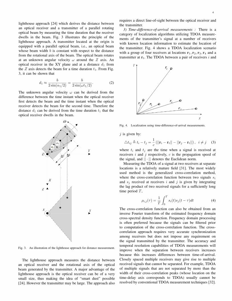
lighthouse approach [24] which derives the distance betweenan optical receiver and a transmitter of a parallel rotatingoptical beam by measuring the time duration that the receiverdwells in the beam. Fig. 3 illustrates the principle of thelighthouse approach. A transmitter located at the origin isequipped with a parallel optical beam, i.e., an optical beamwhose beam width b is constant with respect to the distancefrom the rotational axis of the beam. The optical beam rotatesat an unknown angular velocity ω around the Z axis. Anoptical receiver in the XY plane and at a distance d1 fromthe Z axis detects the beam for a time duration t1. From Fig.3, it can be shown that

d1 ≈ b

2 sin(α1/2)=

b

2 sin(ωt1/2). (2)

The unknown angular velocity ω can be derived from thedifference between the time instant when the optical receiverfirst detects the beam and the time instant when the opticalreceiver detects the beam for the second time. Therefore thedistance d1 can be derived from the time duration t1 that theoptical receiver dwells in the beam.

Fig. 3. An illustration of the lighthouse approach for distance measurement.

The lighthouse approach measures the distance betweenan optical receiver and the rotational axis of the opticalbeam generated by the transmitter. A major advantage of thelighthouse approach is the optical receiver can be of a verysmall size, thus making the idea of “smart dust” possible[24]. However the transmitter may be large. The approach also

requires a direct line-of-sight between the optical receiver andthe transmitter.

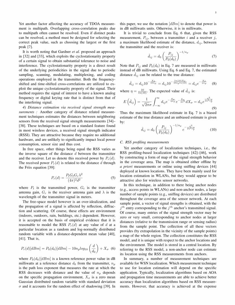
3) Time-difference-of-arrival measurements : There is acategory of localization algorithms utilizing TDOA measure-ments of the transmitter’s signal at a number of receiverswith known location information to estimate the location ofthe transmitter. Fig. 4 shows a TDOA localization scenariowith a group of four receivers at locations r1, r2, r3, r4 and atransmitter at rt. The TDOA between a pair of receivers i and

Fig. 4. Localization using time-difference-of-arrival measurements.

j is given by:

4tij , ti − tj =1c

(||ri − rt|| − ||rj − rt||) , i 6= j (3)

where ti and tj are the time when a signal is received atreceivers i and j respectively, c is the propagation speed ofthe signal, and || · || denotes the Euclidean norm.

Measuring the TDOA of a signal at two receivers at separatelocations is a relatively mature field [31]. The most widelyused method is the generalized cross-correlation method,where the cross-correlation function between two signals si

and sj received at receivers i and j is given by integratingthe lag product of two received signals for a sufficiently longtime period T ,

ρi,j(τ) =1T

∫ T

0

si(t)sj(t− τ)dt (4)

The cross-correlation function can also be obtained from aninverse Fourier transform of the estimated frequency domaincross-spectral density function. Frequency domain processingis often preferred because the signals can be filtered priorto computation of the cross-correlation function. The cross-correlation approach requires very accurate synchronizationamong receivers but does not impose any requirement onthe signal transmitted by the transmitter. The accuracy andtemporal resolution capabilities of TDOA measurements willimprove when the separation between receivers increasesbecause this increases differences between time-of-arrival.Closely spaced multiple receivers may give rise to multiplereceived signals that cannot be separated. For example, TDOAof multiple signals that are not separated by more than thewidth of their cross-correlation peaks (whose location on thetime-delay axis corresponds to TDOA) usually cannot beresolved by conventional TDOA measurement techniques [32].

5

Yet another factor affecting the accuracy of TDOA measure-ment is multipath. Overlapping cross-correlation peaks dueto multipath often cannot be resolved. Even if distinct peakscan be resolved, a method must be designed for selecting thecorrect peak value, such as choosing the largest or the firstpeak [7].

It is worth noting that Gardner et al. proposed an approachin [32] and [33], which exploits the cyclostationarity propertyof a certain signal to obtain substantial tolerance to noise andinterference. The cyclostationarity property is a direct resultof the underlying periodicities in the signal due to periodicsampling, scanning, modulating, multiplexing, and codingoperations employed in the transmitter. Both the frequency-shifted and time-shifted cross-correlations are utilized to ex-ploit the unique cyclostationarity property of the signal. Theirmethod requires the signal of interest to have a known analogfrequency or digital keying rate that is distinct from that ofthe interfering signal.

4) Distance estimation via received signal strength mea-surements : Another category of distance related measure-ment techniques estimates the distances between neighboringsensors from the received signal strength measurements [34]–[38]. These techniques are based on a standard feature foundin most wireless devices, a received signal strength indicator(RSSI). They are attractive because they require no additionalhardware, and are unlikely to significantly impact local powerconsumption, sensor size and thus cost.

In free space, other things being equal the RSS varies asthe inverse square of the distance d between the transmitterand the receiver. Let us denote this received power by Pr(d).The received power Pr(d) is related to the distance d throughthe Friis equation [39]:

Pr(d) =PtGtGrλ

2

(4π)2d2(5)

where Pt is the transmitted power, Gt is the transmitterantenna gain, Gr is the receiver antenna gain and λ is thewavelength of the transmitter signal in meters.

The free-space model however is an over-idealization, andthe propagation of a signal is affected by reflection, diffrac-tion and scattering. Of course, these effects are environment(indoors, outdoors, rain, buildings, etc.) dependent. However,it is accepted on the basis of empirical evidence that it isreasonable to model the RSS Pr(d) at any value of d at aparticular location as a random and log-normally distributedrandom variable with a distance-dependent mean value [40],[41]. That is,

Pr(d)[dBm] = P0(d0)[dBm]− 10nplog10

(d

d0

)+ Xσ (6)

where P0(d0)[dBm] is a known reference power value in dBmilliwatts at a reference distance d0 from the transmitter, np

is the path loss exponent that measures the rate at which theRSS decreases with distance and the value of np dependson the specific propagation environment, Xσ is a zero meanGaussian distributed random variable with standard deviationσ and it accounts for the random effect of shadowing [39]. In

this paper, we use the notation [dBm] to denote that power isin dB milliwatts units. Otherwise, it is in milliwatts.

It is trivial to conclude from Eq. 6 that, given the RSSmeasurement, Pij , between a transmitter i and a receiver j,a maximum likelihood estimate of the distance, dij , betweenthe transmitter and the receiver is:

dij = d0

(Pij

P0(d0)

)−1/np

(7)

Note that Pij and P0(d0) in Eq. 7 are measured in milliwattsinstead of dB milliwatts. Using Eq. 6 and Eq. 7, the estimateddistance dij can be related to the true distance:

dij = dij10−Xσ

10np = dij10−ln(10)Xσ

10npln(10) = dije− Xσ

ηnp (8)

where η = 10ln(10) . The expected value of dij is:

E(dij

)=

1√2πσ

∫ ∞

−∞dije

− Xσηnp e−

Xσ2σ2 dXσ = dije

σ2

2η2n2p

(9)Thus the maximum likelihood estimate in Eq. 7 is a biasedestimate of the true distance and an unbiased estimate is givenby:

dij = d0

(Pij

P0(d0)

)−1/np

e− σ2

2η2n2p (10)

C. RSS profiling measurements

Yet another category of localization techniques, i.e., theRSS profiling-based localization techniques [42]–[46], workby constructing a form of map of the signal strength behaviorin the coverage area. The map is obtained either offline bya priori measurements or online using sniffing devices [44]deployed at known locations. They have been mainly used forlocation estimation in WLANs, but they would appear to beattractive also for wireless sensor networks.

In this technique, in addition to there being anchor nodes(e.g., access points in WLANs) and non-anchor nodes, a largenumber of sample points (e.g., sniffing devices) are distributedthroughout the coverage area of the sensor network. At eachsample point, a vector of signal strengths is obtained, with thejth entry corresponding to the jth anchor’s transmitted signal.Of course, many entries of the signal strength vector may bezero or very small, corresponding to anchor nodes at largerdistances (relative to the transmission range or sensing radius)from the sample point. The collection of all these vectorsprovides (by extrapolation in the vicinity of the sample points)a map of the whole region. The collection constitutes the RSSmodel, and it is unique with respect to the anchor locations andthe environment. The model is stored in a central location. Byreferring to the RSS model, a non-anchor node can estimateits location using the RSS measurements from anchors.

In summary, a number of measurement techniques areavailable for WSN localization. Which measurement techniqueto use for location estimation will depend on the specificapplication. Typically, localization algorithms based on AOAand propagation time measurements are able to achieve betteraccuracy than localization algorithms based on RSS measure-ments. However, that accuracy is achieved at the expense

6

of higher equipment cost. Patwati et al. gave the Cramer-Rao lower bounds for location estimation using TOA, RSSand AOA measurements respectively in [5]. However theCramer-Rao lower bound may be too optimistic when themeasurement error deviates from Gaussian. Moreover theCramer-Rao bound assumes the underlying estimator is anunbiased estimator. This assumption may not be satisfied bymany localization techniques.

III. ONE-HOP LOCALIZATION TECHNIQUES

In this section, we discuss the principles of one-hop lo-calization techniques in which the non-anchor node to belocalized is the one-hop neighbor of a sufficient number ofanchors.

A. AOA based one-hop localization techniques

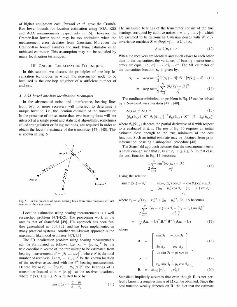
In the absence of noise and interference, bearing linesfrom two or more receivers will intersect to determine aunique location, i.e., the location estimate of the transmitter.In the presence of noise, more than two bearing lines will notintersect at a single point and statistical algorithms, sometimescalled triangulation or fixing methods, are required in order toobtain the location estimate of the transmitter [47], [48]. Thisis shown in Fig. 5

Fig. 5. In the presence of noise, bearing lines from three receivers will notinteract at the same point.

Location estimation using bearing measurements is a wellresearched problem [47]–[52]. The pioneering work in thearea is that of Stansfield [49]. His approach has been fur-ther generalized in [50], [52] and has been implemented inmany practical systems. Another well-known approach is themaximum likelihood estimator [47], [51].

The 2D localization problem using bearing measurementscan be formulated as follows. Let xt = [xt, yt]T be thetrue coordinate vector of the transmitter to be estimated frombearing measurements β = [β1, ..., βN ]T , where N is the totalnumber of receivers. Let xi = [xi, yi]T be the known locationof the receiver associated with the ith bearing measurement.Denote by θ(x) = [θ1(x), ..., θN (x)]T the bearings of atransmitter located at x = [x, y]T at the receiver locations,where θi(x), 1 ≤ i ≤ N is related to x by:

tan θi(x) =y − yi

x− xi(11)

The measured bearings of the transmitter consist of the truebearings corrupted by additive noises ε = [ε1, ..., εN ]T , whichare assumed to be zero-mean Gaussian noises with N × Ncovariance matrices S = diag{σ2

1 , ..., σ2N}, i.e.,

β = θ(xt) + ε (12)

When the receivers are identical and much closer to each otherthan to the transmitter, the variances of bearing measurementerrors are equal, i.e., σ2

1 = · · ·σ2N = σ2. The ML estimator of

the transmitter location xt is given by:

xt = arg min12[θ(xt)− β]T S−1[θ(xt)− β] (13)

= arg min12

N∑

i=1

(θi(xt)− βi)2

σ2i

(14)

The nonlinear minimization problem in Eq. 13 can be solvedby a Newton-Gauss iteration [47], [48]:

xt,k+1 = xt,k + (15)(θx(xt,k)T S−1θx(xt,k)

)−1θx(xt,k)T S−1 [β − θx(xt,k)]

where θx(xt,k) denotes the partial derivative of θ with respectto x evaluated at xt,k. The use of Eq. 15 requires an initialestimate close enough to the true minimum of the costfunction. Such an initial estimate may be obtained from priorinformation, or using a suboptimal procedure [48].

The Stansfield approach assumes that the measurement erroris small enough such that εi ≈ sin εi, 1 ≤ i ≤ N . In that case,the cost function in Eq. 14 becomes:

12

N∑

i=1

sin2(θi(xt)− βi)σ2

i

(16)

Using the relation

sin(θi(xt)− βi) = sin θi(xt) cos βi − cos θi(xt) sin βi

=(yt − yi) cos βi − (xt − xi) sin βi

ri

where ri =√

(xt − xi)2 + (yt − yi)2, Eq. 16 becomes

12

N∑

i=1

[(yt − yi) cos βi − (xt − xi) sin βi]2

σ2i r2

i

=12(Axt − b)T R−1S−1(Axt − b) (17)

where

A =

sinβ1 − cosβ1

......

sin βN − cos βN

(18)

b =

x1 sin β1 − y1 cos β1

...xN sin β1 − y1 cos βN

(19)

R = diag{r21, · · · , r2

N} (20)

Stansfield implicitly assumes that even though R is not per-fectly known, a rough estimate of R can be obtained. Since thecost function weakly depends on R, the fact that the estimate

7

is rough will not significantly affect the solution. Under theseassumptions, the minimization of Eq. 17 with respect to xt isa well known problem and the solution is given by:

xt = (AT R−1S−1A)−1AT R−1S−1b (21)

Note that the closed form solution in the Stansfield approachdepends on two assumptions: first, the measurement error issmall such that εi ≈ sin εi, 1 ≤ i ≤ N ; second, R is known.One may chose to accept the first assumption but reject thesecond assumption. In that case an iterative procedure can beused to obtain the solution to the minimization problem, whichhas no advantage over the ML technique [48].

Analytical expressions for the bias and the covariance ma-trix of the estimation errors associated with the ML approachand with the Stansfield approach were given in [48]. It wasshown that the Stansfield approach provides biased estimateseven for a large number of bearing measurements and theML approach is asymptotically unbiased at a large number ofmeasurements. However the RMS (root mean square) error ofStansfield approach is not necessarily larger than that of theML approach. A quite different approach is referred to at theend of Section III-C, using a very recently introduced methodof exploiting the over-determined nature of the noiselessproblem.

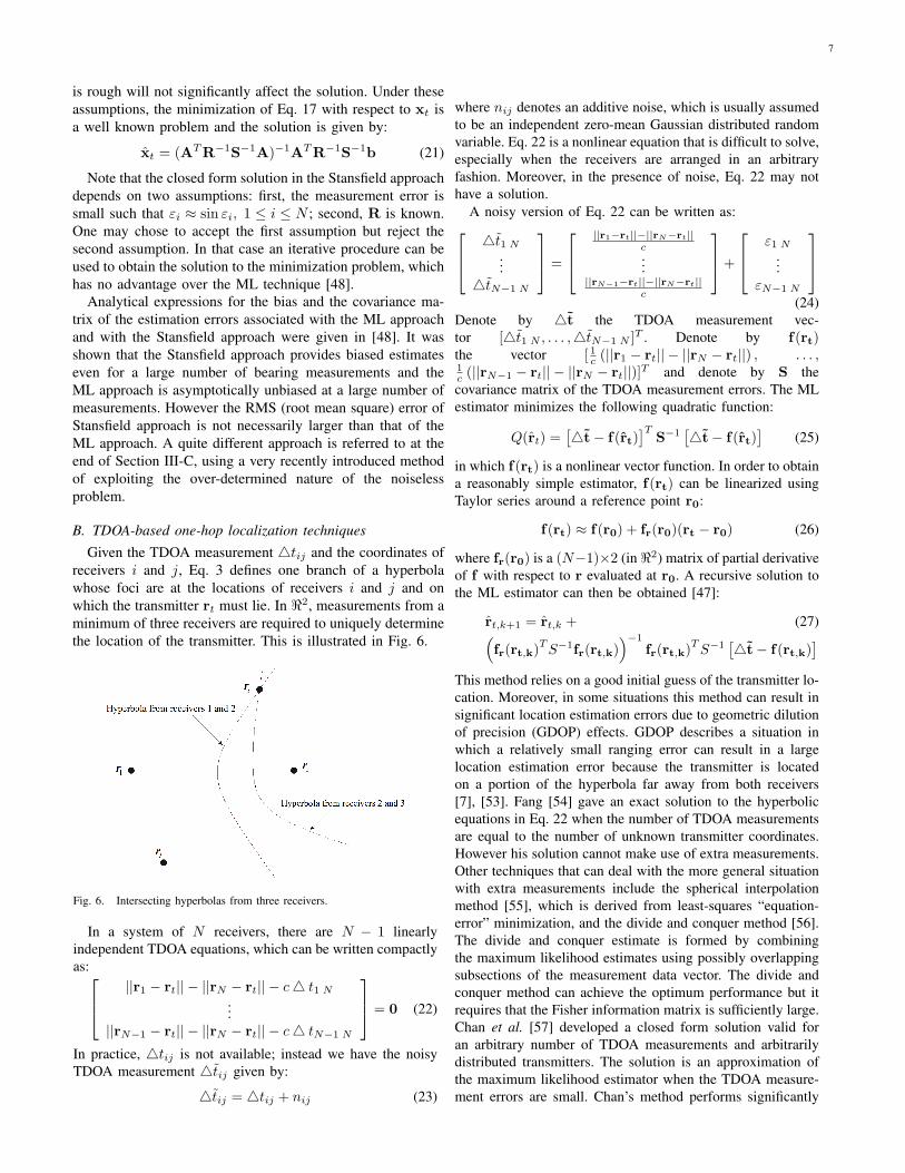
B. TDOA-based one-hop localization techniquesGiven the TDOA measurement 4tij and the coordinates of

receivers i and j, Eq. 3 defines one branch of a hyperbolawhose foci are at the locations of receivers i and j and onwhich the transmitter rt must lie. In <2, measurements from aminimum of three receivers are required to uniquely determinethe location of the transmitter. This is illustrated in Fig. 6.

Fig. 6. Intersecting hyperbolas from three receivers.

In a system of N receivers, there are N − 1 linearlyindependent TDOA equations, which can be written compactlyas:

||r1 − rt|| − ||rN − rt|| − c4 t1 N

...||rN−1 − rt|| − ||rN − rt|| − c4 tN−1 N

= 0 (22)

In practice, 4tij is not available; instead we have the noisyTDOA measurement 4tij given by:

4tij = 4tij + nij (23)

where nij denotes an additive noise, which is usually assumedto be an independent zero-mean Gaussian distributed randomvariable. Eq. 22 is a nonlinear equation that is difficult to solve,especially when the receivers are arranged in an arbitraryfashion. Moreover, in the presence of noise, Eq. 22 may nothave a solution.

A noisy version of Eq. 22 can be written as:

4t1 N

...4tN−1 N

=

||r1−rt||−||rN−rt||c...

||rN−1−rt||−||rN−rt||c

+

ε1 N

...εN−1 N

(24)Denote by 4t the TDOA measurement vec-tor [4t1 N , . . . ,4tN−1 N ]T . Denote by f(rt)the vector [ 1c (||r1 − rt|| − ||rN − rt||) , . . . ,1c (||rN−1 − rt|| − ||rN − rt||)]T and denote by S thecovariance matrix of the TDOA measurement errors. The MLestimator minimizes the following quadratic function:

Q(rt) =[4t− f(rt)

]TS−1

[4t− f(rt)]

(25)

in which f(rt) is a nonlinear vector function. In order to obtaina reasonably simple estimator, f(rt) can be linearized usingTaylor series around a reference point r0:

f(rt) ≈ f(r0) + fr(r0)(rt − r0) (26)

where fr(r0) is a (N−1)×2 (in <2) matrix of partial derivativeof f with respect to r evaluated at r0. A recursive solution tothe ML estimator can then be obtained [47]:

rt,k+1 = rt,k + (27)(fr(rt,k)T

S−1fr(rt,k))−1

fr(rt,k)TS−1

[4t− f(rt,k)]

This method relies on a good initial guess of the transmitter lo-cation. Moreover, in some situations this method can result insignificant location estimation errors due to geometric dilutionof precision (GDOP) effects. GDOP describes a situation inwhich a relatively small ranging error can result in a largelocation estimation error because the transmitter is locatedon a portion of the hyperbola far away from both receivers[7], [53]. Fang [54] gave an exact solution to the hyperbolicequations in Eq. 22 when the number of TDOA measurementsare equal to the number of unknown transmitter coordinates.However his solution cannot make use of extra measurements.Other techniques that can deal with the more general situationwith extra measurements include the spherical interpolationmethod [55], which is derived from least-squares “equation-error” minimization, and the divide and conquer method [56].The divide and conquer estimate is formed by combiningthe maximum likelihood estimates using possibly overlappingsubsections of the measurement data vector. The divide andconquer method can achieve the optimum performance but itrequires that the Fisher information matrix is sufficiently large.Chan et al. [57] developed a closed form solution valid foran arbitrary number of TDOA measurements and arbitrarilydistributed transmitters. The solution is an approximation ofthe maximum likelihood estimator when the TDOA measure-ment errors are small. Chan’s method performs significantly

8

better than the spherical interpolation method and is morerobust against noise than the divide and conquer method. Thecomputational complexity of Chan’s method is comparableto the spherical interpolation method but substantially lessthan the Taylor-series method [47]. Recently, Dogancay andDrake et al. developed a closed form solution for localizationof distant transmitters based on triangulation of hyperbolicasymptotes [58], [59]. The hyperbolic curves are approximatedby linear asymptotes. The solution exhibits some performancedegradation with respect to the maximum likelihood estimatorat low noise levels but outperforms the maximum likelihoodestimator at medium to high noise levels.

C. Distance-based one-hop localization techniquesThe most well-known distance-based localization technique

is based on use of GPS. The GPS space segment consists of24 satellites in the medium earth orbit at a nominal altitude of20, 200km with an orbital inclination of 550. Each satellitecarries several high accuracy atomic clocks and radiates asequence of bits that starts at a precisely known time. Thelocation of a GPS satellite at any particular time instantis known. A GPS receiver located on the earth derives itsdistance to a GPS satellite from the difference of the timea GPS signal is received at the receiver and the time theGPS signal is radiated by the GPS satellite. Ideally, distancemeasurements to three GPS satellites allow the GPS receiverto uniquely determine its position. In reality, four satellites,rather than three, are required because of synchronizationerror in the receiver’s clock. The fourth distance measurementprovides information from which the synchronization error ofthe receiver can be corrected and the receiver’s clock can besynchronized to an accuracy better than 100ns.

Generally in a WSN, for a non-anchor node at unknownlocation xt with noise-contaminated distance measurementsd1, . . . , dN to N anchors at known locations x1, . . . ,xN ,the location estimation problem can be formulated using amaximum likelihood approach as:

xt = arg min[d(xt)− d

]T

S−1[d(xt)− d

](28)

where d is a N × 1 distance measurement vector, d(xt) isalso a N ×1 vector [||xt − x1||, . . . , ||xt − xN ||] and S is thecovariance matrix of the distance measurement errors. Thisminimization problem can be solved using a similar proceduredescribed in Section III-A and Section III-B.

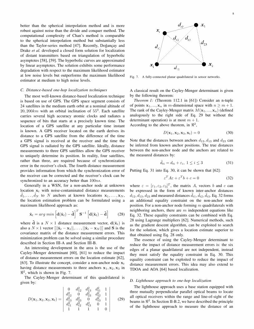
An interesting development in the area is the use of theCayley-Menger determinant [60], [61] to reduce the impactof distance measurement errors on the location estimate [62],[63]. To illustrate the concept, consider a non-anchor node xt

having distance measurements to three anchors x1,x2,x3 in<2, which is shown in Fig. 7.

The Cayley-Menger determinant of this quadrilateral isgiven by:

D(x1,x2,x3,xt) =

∣∣∣∣∣∣∣∣∣∣

0 d212 d2

13 d2t1 1

d212 0 d2

23 d2t2 1

d213 d2

23 0 d2t3 1

d2t1 d2

t2 d2t3 0 1

1 1 1 1 0

∣∣∣∣∣∣∣∣∣∣

(29)

Fig. 7. A fully-connected planar quadrilateral in sensor networks.

A classical result on the Cayley-Menger determinant is givenby the following theorem:

Theorem 1: (Theorem 112.1 in [61]) Consider an n-tupleof points x1, ...,xn in m-dimensional space with n ≥ m + 1.The rank of the Cayley-Menger matrix M(x1, ...,xn) (definedanalogously to the right side of Eq. 29 but without thedeterminant operation) is at most m + 1.According to the above theorem, in <2,

D(x1,x2,x3,xt) = 0 (30)

Note that the distances between anchors d12, d13 and d23 canbe inferred from known anchor positions. The true distancesbetween the non-anchor node and the anchors are related tothe measured distances by:

dti = dti + εi, 1 ≤ i ≤ 3 (31)

Putting Eq. 31 into Eq. 30, it can be shown that [62]:

εT Aε + εT b + c = 0 (32)

where ε = [ε1, ε2, ε3]T , the matrix A, vectors b and c canbe expressed in the form of known inter-anchor distancesd12, d13, d23 and measured distances dt1, dt2, dt3. Eq. 32 formsan additional equality constraint on the non-anchor nodeposition. For a non-anchor node forming m quadrilaterals withneighboring anchors, there are m independent equations likeEq. 32. These equality constraints can be combined with Eq.28 using Lagrange multipliers [62]. Numerical methods, suchas the gradient descent algorithm, can be exploited to searchfor the solution, which gives a location estimate superior tothat obtained using Eq. 28 only.

The essence of using the Cayley-Menger determinant toreduce the impact of distance measurement errors is: the sixedges of a planar quadrilateral are not independent, insteadthey must satisfy the equality constraint in Eq. 30. Thisequality constraint can be exploited to reduce the impact ofdistance measurement errors. This idea may also extend toTDOA and AOA [64] based localization.

D. Lighthouse approach to one-hop localization

The lighthouse approach uses a base station equipped withthree mutually perpendicular parallel optical beams to locateall optical receivers within the range and line-of-sight of thebeams in <3. In Section II-B.2, we have described the principleof the lighthouse approach to measure the distance of an

9

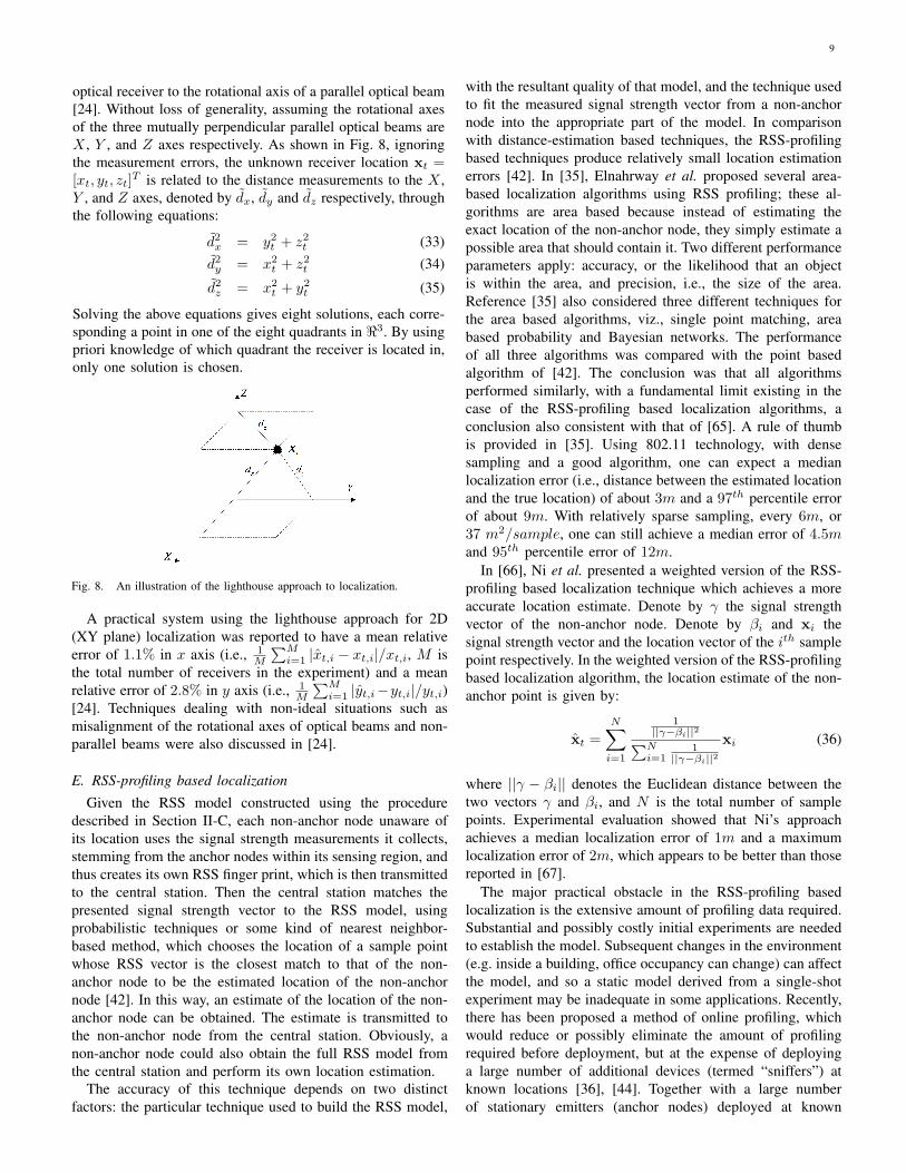
optical receiver to the rotational axis of a parallel optical beam[24]. Without loss of generality, assuming the rotational axesof the three mutually perpendicular parallel optical beams areX , Y , and Z axes respectively. As shown in Fig. 8, ignoringthe measurement errors, the unknown receiver location xt =[xt, yt, zt]T is related to the distance measurements to the X ,Y , and Z axes, denoted by dx, dy and dz respectively, throughthe following equations:

d2x = y2

t + z2t (33)

d2y = x2

t + z2t (34)

d2z = x2

t + y2t (35)

Solving the above equations gives eight solutions, each corre-sponding a point in one of the eight quadrants in <3. By usingpriori knowledge of which quadrant the receiver is located in,only one solution is chosen.

Fig. 8. An illustration of the lighthouse approach to localization.

A practical system using the lighthouse approach for 2D(XY plane) localization was reported to have a mean relativeerror of 1.1% in x axis (i.e., 1

M

∑Mi=1 |xt,i − xt,i|/xt,i, M is

the total number of receivers in the experiment) and a meanrelative error of 2.8% in y axis (i.e., 1

M

∑Mi=1 |yt,i−yt,i|/yt,i)

[24]. Techniques dealing with non-ideal situations such asmisalignment of the rotational axes of optical beams and non-parallel beams were also discussed in [24].

E. RSS-profiling based localization

Given the RSS model constructed using the proceduredescribed in Section II-C, each non-anchor node unaware ofits location uses the signal strength measurements it collects,stemming from the anchor nodes within its sensing region, andthus creates its own RSS finger print, which is then transmittedto the central station. Then the central station matches thepresented signal strength vector to the RSS model, usingprobabilistic techniques or some kind of nearest neighbor-based method, which chooses the location of a sample pointwhose RSS vector is the closest match to that of the non-anchor node to be the estimated location of the non-anchornode [42]. In this way, an estimate of the location of the non-anchor node can be obtained. The estimate is transmitted tothe non-anchor node from the central station. Obviously, anon-anchor node could also obtain the full RSS model fromthe central station and perform its own location estimation.

The accuracy of this technique depends on two distinctfactors: the particular technique used to build the RSS model,

with the resultant quality of that model, and the technique usedto fit the measured signal strength vector from a non-anchornode into the appropriate part of the model. In comparisonwith distance-estimation based techniques, the RSS-profilingbased techniques produce relatively small location estimationerrors [42]. In [35], Elnahrway et al. proposed several area-based localization algorithms using RSS profiling; these al-gorithms are area based because instead of estimating theexact location of the non-anchor node, they simply estimate apossible area that should contain it. Two different performanceparameters apply: accuracy, or the likelihood that an objectis within the area, and precision, i.e., the size of the area.Reference [35] also considered three different techniques forthe area based algorithms, viz., single point matching, areabased probability and Bayesian networks. The performanceof all three algorithms was compared with the point basedalgorithm of [42]. The conclusion was that all algorithmsperformed similarly, with a fundamental limit existing in thecase of the RSS-profiling based localization algorithms, aconclusion also consistent with that of [65]. A rule of thumbis provided in [35]. Using 802.11 technology, with densesampling and a good algorithm, one can expect a medianlocalization error (i.e., distance between the estimated locationand the true location) of about 3m and a 97th percentile errorof about 9m. With relatively sparse sampling, every 6m, or37 m2/sample, one can still achieve a median error of 4.5mand 95th percentile error of 12m.

In [66], Ni et al. presented a weighted version of the RSS-profiling based localization technique which achieves a moreaccurate location estimate. Denote by γ the signal strengthvector of the non-anchor node. Denote by βi and xi thesignal strength vector and the location vector of the ith samplepoint respectively. In the weighted version of the RSS-profilingbased localization algorithm, the location estimate of the non-anchor point is given by:

xt =N∑

i=1

1||γ−βi||2∑N

i=11

||γ−βi||2xi (36)

where ||γ − βi|| denotes the Euclidean distance between thetwo vectors γ and βi, and N is the total number of samplepoints. Experimental evaluation showed that Ni’s approachachieves a median localization error of 1m and a maximumlocalization error of 2m, which appears to be better than thosereported in [67].

The major practical obstacle in the RSS-profiling basedlocalization is the extensive amount of profiling data required.Substantial and possibly costly initial experiments are neededto establish the model. Subsequent changes in the environment(e.g. inside a building, office occupancy can change) can affectthe model, and so a static model derived from a single-shotexperiment may be inadequate in some applications. Recently,there has been proposed a method of online profiling, whichwould reduce or possibly eliminate the amount of profilingrequired before deployment, but at the expense of deployinga large number of additional devices (termed “sniffers”) atknown locations [36], [44]. Together with a large numberof stationary emitters (anchor nodes) deployed at known

10

locations, the “sniffers” can be used to construct and updatethe RSS model online.

F. Localization based on hybrid measurements

There are a number of other localization algorithms basedon data fusion [68] of hybrid measurements. McGuire et al.explored data fusion of RSS and TOA measurements formobile terminal localization in a CDMA cellular network [69].Li et al. considered mobile user localization using hybridTDOA/AOA measurements in a macrocell wideband CDMAsystem with frequency division duplex [70]. Gu et al. con-sidered mobile user localization in a CDMA cellular networkusing hybrid AOA/TOA measurements [71]. Kleine-Ostmannet al. [72] presented a data fusion architecture for combiningTDOA and TOA measurements. Thomas et al. considered thefusion of TDOA and AOA measurements [73]. Catovic [74]computed the Cramer-Rao bounds on the location estimationaccuracy of two different hybrid schemes, i.e., TOA/RSS andTDOA/RSS, and found that hybrid schemes offer improved ac-curacy with respect to conventional TOA and TDOA schemes.Fundamentally, localization based on hybrid measurementscan achieve a performance improvement over that based ona single measurement type because measurement noise fordifferent types of measurements comes from different sources.Therefore errors in the location estimate for each measurementtype are at least partially independent. This independencebetween different types of measurements can be exploited bydata fusion techniques [68] to create estimators that have betteraccuracy than estimators based on single measurement types.Among those hybrid techniques, the fusion of RSS and TOAmeasurements appears to be the most attractive for a WSNbecause of its relatively simple hardware requirement.

IV. NONLINE-OF-SIGHT ERROR MITIGATION

A common problem in many localization techniques isthe nonline-of-sight (NLOS) error mitigation. NLOS errorsbetween two sensors can arise when either the line-of-sightbetween them is obstructed, perhaps by a building, or the line-of-sight measurements are contaminated by reflected and/ordiffracted signals. As NLOS error mitigation in AOA based lo-calization [75]–[77] and distance based localization [78]–[81]share some degree of commonality, we review them together inthis section. Most NLOS error mitigation techniques assumethat NLOS corrupted measurements only constitute a smallfraction of the total measurements. Since NLOS corruptedmeasurements are inconsistent with LOS expectations, theycan be treated as outliers. A typical approach is to assumethat the measurement error has a Gaussian distribution, thenthe least-squares residuals are examined to determine if NLOSerrors are present [76], [80], [81] (by regarding any largeresidual as due to the NLOS signals). Unfortunately, thisapproach fails to work when multiple NLOS measurementsare present as the multiple outliers in the measurement tend tobias the final estimate decision and reduce the residuals. Thisbehavior motivates the use of deletion diagnostics. In deletiondiagnostics, the effects of eliminating various measurementsfrom the total set are computed and ranked [80], [82].

Some other approaches are proposed to reduce estimationerrors for time-of-arrival (TOA) [79], [83] and TDOA [75]respectively when the majority of the measurements are NLOSmeasurements. In [79], Venkatraman et al. employed a con-strained nonlinear optimization approach for TOA NLOS errormitigation in a cellular network. Bounds on the NLOS errorand the relationship between the true ranges are extracted fromthe geometry of the cell layout and the measured range circlesto serve as constraints. Wang et al. proposed an algorithmwhich attempts to mitigate NLOS error effect in a TOAbased location system, utilizing the information that NLOSerror causes the measured distance to be greater than the truedistance. A quadratic programming approach is used to solvefor an ML estimate of the source location [84]. Cong et al.proposed two NLOS error mitigation algorithms assuming afull knowledge of NLOS error distribution (i.e., the proba-bility that each measurement is NLOS and the probabilitydistribution of NLOS error) and a partial knowledge of NLOSerror distribution (i.e., the probability that each measurementis NLOS and the mean value of the probability distribution ofNLOS error) respectively [75]. However this prior informationmay be difficult to obtain in a WSN.

V. CONNECTIVITY BASED MULTIHOP LOCALIZATIONALGORITHMS

In the following sections, we shall review multihop lo-calization techniques in which the non-anchor nodes are notnecessarily the one-hop neighbors of the anchors. In particular,we focus on connectivity-based and distance-based multihoplocalization algorithms due to their prevalence in multihopWSN localization techniques.

There is a distinct category of localization algorithms, calledconnectivity-based or “range free” localization algorithms,which do not rely on any of the measurement techniques in theearlier sections. Instead they use the connectivity information,i.e., “who is within the communications range of whom” [85]to estimate the locations of the non-anchor nodes. The princi-ple of these algorithms is: a sensor being in the transmissionrange of another sensor defines a proximity constraint betweenboth sensors, which can be exploited for localization. Bulusuet al. [86] and Niculescu et al. [87] developed distributedconnectivity-based localization algorithms; Shang et al. [85]and Doherty et al. [88] developed centralized connectivity-based localization algorithms.

In [86], Bulusu et al. defined a connectivity metric, whichis the ratio of the number of transmitter signals successfullyreceived to the total number of signals from that transmit-ter, to measure the quality of communication for a specifictransmitter-receiver pair. A receiver at an unknown locationuses the centroid of its reference points as its location estimate,where a reference point is a transmitter with a known locationand whose connectivity metric exceeds a certain threshold(90% in [86]). An experiment was conducted in a 10m×10moutdoor parking lot using four reference points placed at thefour corners of the 10m × 10m square. The 10m × 10msquare was subdivided into 100 smaller 1m×1m grids and thereceivers were placed at the grid points. Experimental results

11

showed that for over 90% of the data points the localizationerror falls within 30% of the separation distance between twoadjacent reference points.

The “DV(distance vector)-hop” approach developed byNiculescu et al. [87] starts with all anchors flooding theirlocations to other nodes in the network. The messages arepropagated hop-by-hop and there is a hop-count in the mes-sage. Each node maintains an anchor information table andcounts the least number of hops that it is away from an anchor.When an anchor receives a message from another anchor, itestimates the average distance of one hop using the locationsof both anchors and the hop-count, and sends it back to thenetwork as a correction factor. When receiving the correctionfactor, a non-anchor node is able to estimate its distance toanchors and performs trilateration to estimate its location. Thealgorithm was tested using simulation with a total of 100 nodesuniformly distributed in a circular region of diameter 10. Theaverage node degree, i.e., average number of neighbors pernode, is 7.6. Simulation results showed that the algorithm hasa mean error of 45% transmission range with 10% anchors;and has a reduced mean error of about 30% transmission rangewhen the percentage of anchors increases above 20%.

Shang et al. [85] developed a centralized algorithm by usingmulti-dimensional scaling (MDS). MDS was originally usedin psychometrics and psychophysics and it is a set of dataanalysis techniques that displays the structure of distance-likedata as a geometric picture. In their algorithm, the shortestpaths (i.e., the number of hops) between all pairs of nodes arefirst computed, which are used to construct a distance matrixfor MDS. Then MDS is applied to the distance matrix andan approximate value of the relative coordinates of each nodeis obtained. Finally, the relative coordinates are transformedto the absolute coordinates by aligning the estimated relativecoordinates of anchors with their absolute coordinates. Thelocation estimates obtained using earlier steps can be refinedusing a least-squares minimization. Simulation was conductedusing 100 nodes uniformly distributed in a square of size10×10 and four anchors were randomly placed in the region.The average node degree is 10. Simulation results showeda localization error of 0.35. Shang et al. further improvedtheir algorithm in [89] by dividing the entire sensor networkinto overlapping local regions. Localization is performed inindividual regions using the earlier described procedures. Thenthese local maps are patched together to form a global mapby using common nodes shared between adjacent regions.The improved algorithm can achieve better performance onirregularly-shaped networks by avoiding the use of distanceinformation between far away nodes. The improved algorithmcan also be implemented in a distributed fashion.

In the centralized algorithm of Doherty et al. [88], theconnectivity-based localization problem is formulated as aconvex optimization problem and solved using existing al-gorithms for solving linear programs and semidefinite pro-gramming (SDP) algorithms. Semidefinite programs are a

generalization of the linear programs and have the form:

Minimize cT x (37)Subject to: F(x) = F0 + x1F1 + · · ·+ xnFn (38)

Ax < b (39)Fi = FT

i (40)

where x = [x1,x2, ...,xn]T and xi represents the coordinatevector of node i, i.e., xi = [xi, yi]. The quantities A, b,c and Fi are all known. The inequality 39 is known as alinear matrix inequality. A connection between node i andj can be represented by a “radial constraint” on the nodelocations: ||xi−xj || ≤ R, where R is the transmission range.This constraint is a convex constraint and can be transformedinto a LMI using Schur complements [88]. A solution tothe coordinates of the non-anchor nodes satisfying the radialconstraints can be obtained by leaving the objective functioncT x blank and solving the problem. Because there may bemany possible coordinates of the non-anchor nodes satisfyingthe constraints, the solution may not be unique. If we set theelement of c corresponding to xi (or yi) to be 1 (or -1) andall other elements of c to be zero, the problem becomes aconstrained maximization (or minimization) problem. A lowerbound or an upper bound on xi (or yi) satisfying the radialconstraints can be computed, from which a rectangular boxbounding the location estimates of the non-anchor nodes canbe obtained. The algorithm was tested using simulation witha total of 200 nodes randomly placed in a square of size10R×10R and the average node degree is 5.7 [88]. Simulationresults showed that the mean location error is a monotonicallydecreasing function of the number of anchors. When thenumber of anchors is small, the estimated location is as poor asa random guess of the node’s coordinates. The mean locationerror reduces to R when the number of anchors increases to18; it reduces to 0.5R when the number of anchors increasesto 50.

In comparison with other localization algorithms, the mostattractive feature of the connectivity-based localization algo-rithms is their simplicity. However they can only providea coarse grained estimate of each node’s location, whichmeans that they are only suitable for applications requiringan approximate location estimate only. Also the localizationerror is highly dependent on the node density of the network,the number of anchors and the network topology. The locationerror will be larger in a network with a smaller node density,fewer anchors, or irregular network topology.

VI. DISTANCE-BASED MULTIHOP LOCALIZATIONALGORITHMS

The core of distance-based localization algorithms is the useof inter-sensor distance measurements in a sensor network tolocate the entire network. Based on the approach of process-ing the individual inter-sensor distance data, distance-basedlocalization algorithms can be considered in two main classes:centralized algorithms and distributed algorithms. Centralizedalgorithms use a single central processor to collect all theindividual inter-sensor distance data and produce a map ofthe entire sensor network, while distributed algorithms rely

12

on self-localization of each node in the sensor network usingthe distances the node measures and the local informationit collects from its neighbors. Next we review the maincharacteristics as well as relevant studies in the literature foreach of the two classes and compare them at the end of thesection.

A. Centralized algorithmsIn certain networks where a centralized information archi-

tecture already exists, such as road traffic monitoring andcontrol, environmental monitoring, health monitoring, andprecision agriculture monitoring networks, the measurementdata of all the nodes in the network are collected in a centralprocessor unit. In such a network, it is convenient to use acentralized localization scheme.

Once feasible to implement, the main motive behind theinterest in centralized localization schemes is the likelihood ofproviding more accurate location estimates than those providedby distributed algorithms. In the literature, there exist threemain approaches for designing centralized distance-based lo-calization algorithms: multidimensional scaling (MDS), linearprogramming and stochastic optimization approaches.

The MDS approach used in the connectivity-based local-ization algorithms mentioned in Section V, e.g., [85], can bereadily extended to incorporate distance measurements intothe corresponding optimization problem. Such an extension ofthe algorithm in [85] using the MDS approach can be foundin [90]. In this work, the whole sensor network is dividedinto smaller groups where adjacent groups may share commonsensors. Each group contains at least three anchors or sensorswhose locations have already been estimated. MDS is usedto estimate the relative locations of sensors in each groupand build local maps. Local maps are then stitched togetherto form an estimated global map of the network by utilizingcommon sensors between adjacent local maps. The estimatedlocations of the anchors in this estimated global map arelater iteratively aligned with the true locations of anchors toobtain the final estimated global map. Although this algorithmappears to have a distributed architecture, since a large numberof iterations (implies a high communication cost) are requiredfor the algorithm to converge, it is more appropriate to beimplemented using a centralized architecture. Ji’s algorithmwas tested using a total of 400 nodes (10% anchors) uniformlydistributed in a square of 100× 100 and a transmission rangeof R = 10. The distance measurement error was assumed tobe uniformly distributed in the range [0, η]. It was shown thatwhen η is 0, 0.05R, 0.25R and 0.5R, the localization error is0.1R, 0.15R, 0.3R and 0.45R respectively.

Similarly to the MDS approach, the semi-definite program-ming (SDP) approach used for connectivity-based localiza-tion algorithms can also be extended to incorporate distancemeasurements [88]. In [91] the distance-based sensor networklocalization problem is formulated in a quadratic form andsolved using SDP; and in [92] the result in [91] is improvedusing a gradient search procedure to fine-tune the initialsolution obtained using SDP.

The stochastic optimization approach suggests an alternativeformulation and solution of the distance-based localization

problem using combinatorial optimization notions and tools.The main tool used in this approach is the simulated annealing(SA) technique [93], which is a generalization of the wellknown Monte Carlo method in combinatorial optimization.One particular property of the SA method is its robustnessagainst converging to a false local minimum. In order to applythis tool to the problem of localizing a sensor network with manchor nodes numbered from 1 to m and n non-anchor nodesnumbered from m+1 to m+n, the location estimation problemis reformulated in an optimization framework as minimizationof the cost function

J =m+n∑

i=m+1

∑

j∈Ni

(‖xi − xj‖ − dij

)2

(41)

over {xi|m + 1 ≤ i ≤ m + n} , where Ni, xi and dij denote,respectively, the neighborhood of node i, the estimate of thelocation xi of node i, and the measured distance between nodesi and j.

An algorithm to solve the above optimization problem usingthe SA method is provided in [93]. The performance of thisalgorithm is improved in [94] utilizing the information aboutthe sensor locations hidden in the knowledge of whether agiven pair of sensors are neighbors and mitigating a certainkind of localization error caused by flip ambiguity, a conceptwhich is described in detail in Section VII. The effectivenessof the enhanced algorithm in [94] is also demonstrated viasimulations where the relation between the actual value dij

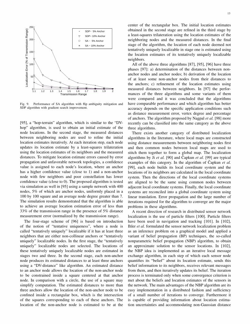
and the measured value dij of the distance between nodes iand j is assumed to be dij = dij(1 + 0.1ξij), where ξij is azero-mean Gaussian noise of unit variance. The simulationswere performed in a sensor network of 200 nodes uniformlydistributed in a square of size 10 by 10. The results of thesesimulations were compared with the ones obtained using theSDP approach with gradient search improvement [92] in Fig.9, where the location estimation error is normalized by thetransmission range. As can be seen in the figure, the SAalgorithm has better accuracy than the SDP algorithm withgradient search. This is an expected result of robustness ofSA against convergence to false local minima; however it isworth noting that the computational cost of the SA approachis higher.

B. Distributed Localization

Similarly to the centralized ones, the distributed distance-based localization approaches can be obtained as an extensionof the distributed connectivity-based localization algorithmsin Section V to incorporate the available inter-sensor distanceinformation. In [87], after developing the “DV-hop” algorithmdescribed in Section V, a modified version of this algorithmwhich includes distance measurements into the localizationprocess, the “DV-distance” algorithm, is presented as well.The main idea in the “DV-distance” algorithm as compared tothe “DV-hop” algorithm is propagation of measured distanceamong neighboring nodes instead of hop count.

Two similar approaches are the two-stage localizationscheme of Savarese et al. [95] and the four-stage algorithmof Savvides et al. [96]. In the first stage of the scheme in

13

1.1 1.2 1.3 1.4 1.5 1.6 1.7 1.8 1.9 20

50

100

150

200

250

Transmission Range

Loca

lizat

ion

Err

or (

% o

f Tra

nsm

issi

on R

ange

)

SDP− 5% Anchor

SDP− 10% Anchor

SA − 5% Anchor

SA − 10% Anchor

Fig. 9. Performance of SA algorithm with flip ambiguity mitigation andSDP algorithm with gradient search improvement.

[95], a “hop-terrain” algorithm, which is similar to the “DV-hop” algorithm, is used to obtain an initial estimate of thenode locations. In the second stage, the measured distancesbetween neighboring nodes are used to refine the initiallocation estimates iteratively. At each iteration step, each nodeupdates its location estimate by a least-squares trilaterationusing the location estimates of its neighbors and the measureddistances. To mitigate location estimate errors caused by errorpropagation and unfavorable network topologies, a confidencevalue is assigned to each node’s location, where an anchorhas a higher confidence value (close to 1) and a non-anchornode with few neighbors and poor constellation has lowerconfidence value (close to 0). The proposed algorithm is testedvia simulation as well in [95] using a sample network with 400nodes, 5% of which are anchor nodes, uniformly placed in a100 by 100 square and an average node degree greater than 7.The simulation results demonstrated that the algorithm is ableto achieve an average location estimation error of less than33% of the transmission range in the presence of 5% distancemeasurement error (normalized by the transmission range).

The four-stage scheme of [96] is based on introductionof the notion of “tentative uniqueness”, where a node iscalled “tentatively uniquely” localizable if it has at least threeneighbors that are either non-collinear anchors or “tentativelyuniquely” localizable nodes. In the first stage, the “tentativelyuniquely” localizable nodes are selected. The locations ofthese tentatively uniquely localizable nodes are estimated instages two and three. In the second stage, each non-anchornode produces its estimated distances to at least three anchorsusing a “DV-distance” like algorithm. An estimated distanceto an anchor node allows the location of the non-anchor nodeto be constrained inside a square centered at that anchornode. In comparison with a circle, the use of a square maysimplify computation. The estimated distances to more thanthree anchors allow the location of the non-anchor node to beconfined inside a rectangular box, which is the intersectionof the squares corresponding to each of these anchors. Thelocation of the non-anchor node is estimated to be at the

center of the rectangular box. The initial location estimatesobtained in the second stage are refined in the third stage bya least-squares trilateration using the location estimates of theneighboring nodes and the measured distances. In the finalstage of the algorithm, the location of each node deemed nottentatively uniquely localizable in stage one is estimated usingthe location estimates of its tentatively uniquely localizableneighbors.

All of the above three algorithms [87], [95], [96] have threephases [97]: a) determination of the distances between non-anchor nodes and anchor nodes; b) derivation of the locationof at least some non-anchor nodes from their distances tothe anchors; c) refinement of the location estimates usingmeasured distances between neighbors. In [97] the perfor-mances of the three algorithms and some variants of themwere compared and it was concluded that the algorithmshave comparable performance and which algorithm has betteraccuracy depends on the specific application conditions suchas distance measurement error, vertex degree and percentageof anchors. The algorithm proposed by Nagpal et al. [98] morerecently can be classified into the same category as the abovethree algorithms.

There exists another category of distributed localizationalgorithms in the literature, where local maps are constructedusing distance measurements between neighboring nodes firstand then common nodes between local maps are used tostitch them together to form a global map. The localizationalgorithms by Ji et al. [90] and Capkun et al. [99] are typicalexamples of this category. In the algorithm of Capkun et al.[99], each node builds its local coordinate system and thelocations of its neighbors are calculated in the local coordinatesystem. Then the directions of the local coordinate systemsare aligned to be the same using common nodes betweenadjacent local coordinate systems. Finally, the local coordinatesystems are reconciled into a global coordinate system usinglinear translation. Error propagation and the large number ofiterations required for the algorithm to converge are the majorproblems in these algorithms.

A recent direction of research in distributed sensor networklocalization is the use of particle filters [100]. Particle filtershave been used in navigation and tracking [101]. In [102],Ihler et al. formulated the sensor network localization problemas an inference problem on a graphical model and applied avariant of belief propagation (BP) techniques, the so-callednonparametric belief propagation (NBP) algorithm, to obtainan approximate solution to the sensor locations. In [102],the NBP idea is implemented as an iterative local messageexchange algorithm, in each step of which each sensor nodequantifies its “belief” about its location estimate, sends thisbelief information to its neighbors, receives relevant messagesfrom them, and then iteratively updates its belief. The iterationprocess is terminated only when some convergence criterion ismet about the beliefs and location estimates of the sensors inthe network. The main advantages of the NBP algorithm are itseasy implementation in a distributed fashion and sufficiencyof a small number of iterations to converge. Furthermore itis capable of providing information about location estima-tion uncertainties and accommodating non-Gaussian distance

14

measurement errors. It is demonstrated via simulations [102]that the overall performance of NBP is comparable to thatof a centralized MAP (maximum a posteriori) estimate. Somefuture research directions to further improve the NBP approachcan be found in [102].

C. Centralized versus Distributed Algorithms

Centralized and distributed distance-based localization al-gorithms can be compared from perspectives of locationestimation accuracy, implementation and computation issues,and energy consumption. It is worth noting that decentralizedlocalization is strictly harder than centralized, i.e., any algo-rithm for decentralized localization can always be applied tocentralized problems, but not the reverse.

From the perspective of location estimation accuracy, cen-tralized algorithms are likely to provide more accurate locationestimates than distributed algorithms. However centralizedalgorithms suffer from the scalability problem and generallyare not feasible to be implemented for large scale sensornetworks. Other disadvantages of centralized algorithms, ascompared to distributed algorithms, are their requirement ofhigher computational complexity and lower reliability due toaccumulated information inaccuracies/losses caused by multi-hop transmission over a wireless network.

On the other hand, distributed algorithms are more difficultto design because of the potentially complicated relationshipbetween local behavior and global behavior, e.g., algorithmsthat are locally optimal may not perform well in a globalsense. Optimal distribution of the computation of a centralizedalgorithm in a distributed implementation in general is anunsolved research problem. Error propagation is another po-tential problem in distributed algorithms. Moreover, distributedalgorithms generally require multiple iterations to arrive astable solution which may cause the localization process totake longer time than the acceptable in some cases.

To compare the centralized and distributed distance-basedlocalization algorithms from the communication energy con-sumption perspective, one needs to consider the individualamounts of energy required for each type of operation in thelocalization algorithm in the specific hardware and the trans-mission range setting. Depending on the setting, the energyrequired for transmitting a single bit could be used to execute1,000 to 2,000 instructions [103]. Centralized algorithms inlarge networks require each sensor’s measurements to be sentover multiple hops to a central processor, while distributedalgorithms require only local information exchange betweenneighboring nodes but many such local exchanges may berequired, depending on the number of iterations needed toarrive at a stable solution. A comparison of the communicationenergy efficiencies of centralized and distributed algorithmscan be found in [104]. It was concluded in [104] that ingeneral, if in a given sensor network and distributed algorithm,the average number of hops to the central processor exceedsthe necessary number of iterations, then the distributed algo-rithm will be more energy-efficient than a typical centralizedalgorithm.

VII. GRAPH THEORETIC RESEARCH PROBLEMS INDISTANCE-BASED SENSOR NETWORK LOCALIZATION

Despite a significant number of approaches developed forWSN localization, there are still many unsolved problemsin the area. The challenges to be addressed are both inanalytical characterization of the sensor networks (from theaspect of localization) and development of (efficient) localiza-tion algorithms for various classes of sensor networks undera variety of conditions. In this section, we present someof these research problems with a discussion on possibleapproaches to them. Although these problems may also existin localization using other types of measurement techniques(e.g., TDOA and AOA), we focus on distance-based sensornetwork localization.

A fundamental problem in distance-based sensor networklocalization is whether a given sensor network is uniquelylocalizable or not. A framework that is useful for analyzing andsolving the problem is graph theory [105]–[109]. In a graphtheoretical framework, a sensor network can be represented bya graph G = (V,E) with a vertex set V and an edge set E,where each vertex i ∈ V is associated with a sensor node si inthe network, and each edge (i, j) ∈ E corresponds to a sensorpair si, sj for which the inter-sensor distance dij is known.The location information about the sensors corresponds to arepresentation of the representative graph. In general, a d-dimensional (d ∈ {2, 3}) representation of a graph G = (V,E)is a mapping p : V → <d, which assigns a location in <d

to each vertex in V . Given a graph G = (V,E) and a d-dimensional representation of it, the pair (G, p) is called ad-dimensional framework.

A particular graph property associated with unique local-izability of sensor networks is global rigidity [106], [108],[109]. A framework (G, p) is globally rigid if every framework(G, p1) satisfying ‖ p(i) − p(j) ‖=‖ p1(i) − p1(j) ‖ forany vertex pair i, j ∈ V , which are connected by an edge inE, also satisfies the same equality for any other vertex pairsthat are not connected by a single edge. A relaxed form ofglobal rigidity is rigidity: A framework (G, p) is rigid if thereexists a sufficiently small positive constant ε such that everyframework (G, p1) satisfying (i) ‖p(i) − p1(i)‖ < ε for alli ∈ V and (ii) ‖ p(i) − p(j) ‖=‖ p1(i) − p1(j) ‖ for anyvertex pair i, j ∈ V , which are connected by an edge in E,also satisfies the equality in (ii) for any other vertex pairs thatare not connected by a single edge.

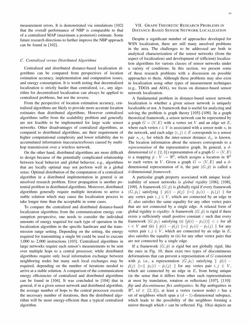
If a framework (G, p) is rigid but not globally rigid, likethe ones in Fig. 10, there exist two types of discontinuousdeformations that can prevent a representation of G consistentwith p, i.e., a representation (G, p1) satisfying ‖ p(i) −p(j) ‖=‖ p1(i) − p1(j) ‖ for any vertex pair i, j ∈ V ,which are connected by an edge in E, from being unique(in the sense that it differs from other such representationsat most by translation, rotation or reflection) [107], [110]:flip and discontinuous flex ambiguities. In flip ambiguities in<d, (d ∈ {2, 3}), at least a vertex (sensor node) v has aset of neighbors which span a (d− 1)-dimensional subspace,which leads to the possibility of the neighbors forming amirror through which v can be reflected. Fig. 10(a) depicts an

15

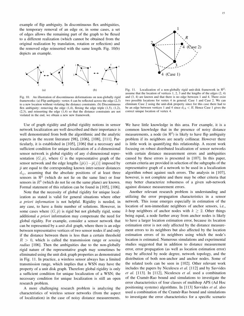
example of flip ambiguity. In discontinuous flex ambiguities,the temporary removal of an edge or, in some cases, a setof edges allows the remaining part of the graph to be flexedto a different realization (which cannot be obtained from theoriginal realization by translation, rotation or reflection) andthe removed edge reinserted with the same length. Fig. 10(b)depicts an example.

(a)2

14

3

2

1 4

3

(a)

2

41

1

3

5

2

4

3

5

(b)

Fig. 10. An illustration of discontinuous deformations on non-globally rigidframeworks: (a) Flip ambiguity: vertex 4 can be reflected across the edge (2,3)to a new location without violating the distance constraints. (b) Discontinuousflex ambiguity: removing the edge (1,4), flexing the edge triple (1,5), (1,2),(2,3), and reinserting the edge (1,4) so that the distance constraints are notviolated in the end, we obtain a new new framework.

Use of graph rigidity and global rigidity notions in sensornetwork localization are well described and their importance iswell demonstrated from both the algorithmic and the analyticaspects in the recent literature [98], [106], [108], [111]. Par-ticularly, it is established in [105], [106] that a necessary andsufficient condition for unique localization of a d-dimensionalsensor network is global rigidity of any d-dimensional repre-sentation (G, p), where G is the representative graph of thesensor network and the edge lengths ‖p(i)− p(j)‖ imposed byp are equal to the corresponding known inter-sensor distancesdij , assuming that the absolute positions of at least threesensors in <2 (which do not lie on the same line) or foursensors in R3 (which do not lie on the same plane) are known.Formal statement of this relation can be found in [105], [106].

Note that the necessity of global rigidity for unique local-ization as stated is valid for general situations where othera priori information is not helpful. Rigidity is needed, inany case, to have a finite number of solutions. However, insome cases where (G, p) is rigid but not globally rigid, someadditional a priori information may compensate the need forglobal rigidity. For example, consider a sensor network thatcan be represented by a unit disk graph, where there is an edgebetween representative vertices of two sensor nodes if and onlyif the distance between them is less than a certain thresholdR > 0, which is called the transmission range or sensingradius [106]. Then the ambiguities due to the non-globallyrigid nature of the representative graph may sometimes beeliminated using the unit disk graph properties as demonstratedin Fig. 11. In practice, a wireless sensor always has a limitedtransmission range, which implies that a WSN may have theproperty of a unit disk graph. Therefore global rigidity is onlya sufficient condition for unique localization of a WSN; thenecessary condition for unique localization is still an openresearch problem.

A more challenging research problem is analyzing thecharacteristics of wireless sensor networks (from the aspectof localization) in the case of noisy distance measurements.

3

2

4 (Case 2)

1

4 (Case 1)

R

Fig. 11. Localization of a non-globally rigid unit-disk framework in <2:assume that the location of vertices 1, 2, 3 and the lengths of the edges (2, 4)and (3, 4) are known and that there is no edge between 1 and 4. There existtwo possible locations for vertex 4 in general: Case 1 and Case 2. We caneliminate Case 2 using the unit-disk property since for this case there had tobe an edge between vertices 1 and 4 since d14 < R. Hence Case 1 gives thecorrect unique location of vertex 4.

We have little knowledge in this area. For example, it is acommon knowledge that in the presence of noisy distancemeasurements, a node (in <2) is likely to have flip ambiguityproblem if its neighbors are nearly collinear. However thereis little work in quantifying this relationship. A recent workfocusing on robust distributed localization of sensor networkswith certain distance measurement errors and ambiguitiescaused by these errors is presented in [107]. In this paper,certain criteria are provided in selection of the subgraphs of therepresentative graph of a network to be used in a localizationalgorithm robust against such errors. The analysis in [107],however, is not complete and there may be other criteria thatmay better characterize robustness of a given sub-networkagainst distance measurement errors.

Another relevant research problem is understanding andutilizing the error propagation characteristics in a sensornetwork. This issue emerges especially in estimation of thelocation of non-immediate neighbors of anchor sensors, i.e.,k-hop neighbors of anchor nodes with k ≥ 2. Other thingsbeing equal, a node further away from anchor nodes is likelyto have a larger location estimation error, because its locationestimation error is not only affected by the distance measure-ment errors to its neighbors but also affected by the locationestimation errors of its neighbors using which the node’slocation is estimated. Numerous simulations and experimentalstudies suggested that in addition to distance measurementerror, error propagation (as well as location estimation error)may be affected by node degree, network topology, and thedistribution of both non-anchor and anchor nodes. Some ofthe related tools can be seen in [102]. Other relevant workincludes the papers by Niculescu et al. [112] and by Savvideset al. [113]. In [112], Niculescu et al. used a combinationof the Cramer-Rao bound and simulations to investigate theerror characteristics of four classes of multihop APS (Ad Hocpositioning systems) algorithms. In [113] Savvides et al. alsoused a combination of the Cramer-Rao bound and simulationsto investigate the error characteristics for a specific scenario

16

in which anchors are located near the boundary of the regionand non-anchor nodes are located inside the region. Somequalitative trends on how localization error varies with averagenode degree, number of anchors and distance to anchors areobserved. A potential problem with using the Cramer-Raobound to study the performance of a localization algorithm isthat the Cramer-Rao bound assumes the underlying estimatoris unbiased. This assumption needs to be validated with theestimators used in various localization algorithms, and inparticular, the class of algorithms which minimize the sum ofthe square of the difference between measured distances andestimated distances. The aforementioned flip ambiguity anddiscontinuous flex ambiguity problems make such validationparticularly difficult. An estimator may produce an unbiasedestimate in one topology (e.g., a dense network with high nodedegree) but give a biased estimate in another topology (e.g., aspare network with low node degree). We are yet to developmore comprehensive knowledge in this large and fascinatingarea.

Still another research area is concerned with reducing thecomputational complexity of location algorithms. It is con-cluded in the literature that the computational complexity ofan arbitrary location procedure is, in general, exponential inthe number of sensor nodes, unless an iterative procedure isapplied to sensor networks with certain classes of representa-tive graphs such as trilateration and quadrilateration graphs[105], [106], [108]. Since trilateration and quadrilaterationrepresentative graphs provide proven reduced computationalcomplexity in localization and actually there are systematicmethods to locate networks with such representative graphs, itis of interest to develop mechanisms to make these methodsapplicable for certain other classes of representative graphs aswell.

Finally, we note current interest in characterizing statisticalproperties of random sensor networks which will ensure, atleast with high probability, that the network is localizable,or even possesses trilateration structure, so that localizationcomputations are straightforward and indeed decentralizable[105], [108], [114].

VIII. SUMMARY

Wireless sensor network localization has attracted signifi-cant research interest. This interest is expected to grow furtherwith the proliferation of wireless sensor network applications.This paper has provided a review of the measurement tech-niques in WSN localization and the corresponding localizationalgorithms. These localization algorithms were divided intoone-hop localization algorithms and multi-hop localizationalgorithms. A detailed investigation on connectivity-based anddistance-based localization algorithms were presented becauseof their popularity in wireless sensor network localization.Despite significant research developments in the area, thereare still quite many unsolved problems in wireless sensor net-work localization. A discussion on some fundamental researchproblems in distance-based location and possible approachesto these problem was also presented in this paper.

ACKNOWLEDGMENT

The authors would like to thank the anonymous reviewersfor their helpful comments which have significantly improvedthe quality of the paper.

REFERENCES

[1] C.-Y. Chong and S. Kumar, “Sensor networks: evolution, opportunities,and challenges,” Proceedings of the IEEE, vol. 91, no. 8, pp. 1247–1256, 2003.

[2] S. Guolin, C. Jie, G. Wei, and K. J. R. Liu, “Signal processingtechniques in network-aided positioning: a survey of state-of-the-artpositioning designs,” IEEE Signal Processing Magazine, vol. 22, no. 4,pp. 12–23, 2005.

[3] A. H. Sayed, A. Tarighat, and N. Khajehnouri, “Network-based wire-less location: challenges faced in developing techniques for accuratewireless location information,” IEEE Signal Processing Magazine,vol. 22, no. 4, pp. 24–40, 2005.

[4] F. Gustafsson and F. Gunnarsson, “Mobile positioning using wirelessnetworks: possibilities and fundamental limitations based on availablewireless network measurements,” IEEE Signal Processing Magazine,vol. 22, no. 4, pp. 41–53, 2005.

[5] N. Patwari, J. Ash, S. Kyperountas, I. Hero, A.O., R. Moses, andN. Correal, “Locating the nodes: cooperative localization in wirelesssensor networks,” IEEE Signal Processing Magazine, vol. 22, no. 4,pp. 54–69, 2005.

[6] D. Koks, “Numerical calculations for passive geolocation scenarios,Tech. Rep. DSTO-RR-0000, 2005.

[7] T. Rappaport, J. Reed, and B. Woerner, “Position location usingwireless communications on highways of the future,” IEEE Communi-cations Magazine, vol. 34, no. 10, pp. 33–41, 1996.

[8] T. E. Biedka, J. H. Reed, and B. D. Woerner, “Direction findingmethods for CDMA systems,” in Thirteenth Asilomar Conference onSignals, Systems and Computers, vol. 1, 1996, pp. 637–641.

[9] D. W. Bliss and K. W. Forsythe, “Angle of arrival estimation in thepresence of multiple access interference for CDMA cellular phone sys-tems,” in Proceedings of the 2000 IEEE Sensor Array and MultichannelSignal Processing Workshop, 2000, pp. 408–412.

[10] I. Ziskind and M. Wax, “Maximum likelihood localization of multiplesources by alternating projection,” IEEE Transactions on Acoustics,Speech, and Signal Processing, vol. 36, no. 10, pp. 1553–1560, 1988.

[11] L. Jian, B. Halder, P. Stoica, and M. Viberg, “Computationally efficientangle estimation for signals with known waveforms,” IEEE Transac-tions on Signal Processing, vol. 43, no. 9, pp. 2154–2163, 1995.

[12] B. Halder, M. Viberg, and T. Kailath, “An efficient non-iterative methodfor estimating the angles of arrival of known signals,” in The Twenty-Seventh Asilomar Conference on Signals, Systems and Computers,1993, pp. 1396–1400.

[13] B. G. Agee, “Copy/DF approaches for signal specific emitter location,”in Conference Record of the Twenty-Fifth Asilomar Conference onSignals, Systems and Computers, vol. 2, 1991, pp. 994–999.

[14] R. Schmidt, “Multiple emitter location and signal parameter estima-tion,” IEEE Transactions on Antennas and Propagation, vol. 34, no. 3,pp. 276–280, 1986.

[15] R. Roy and T. Kailath, “ESPRIT-estimation of signal parameters viarotational invariance techniques,” IEEE Transactions on Acoustics,Speech, and Signal Processing, vol. 37, no. 7, pp. 984–995, 1989.

[16] A. Paulraj, R. Roy, and T. Kailath, “A subspace rotation approach tosignal parameter estimation,” Proceedings of the IEEE, vol. 74, no. 7,pp. 1044–1046, 1986.

[17] N. Tayem and H. M. Kwon, “Conjugate ESPRIT (C-SPRIT),” IEEETransactions on Antennas and Propagation, vol. 52, no. 10, pp. 2618–2624, 2004.

[18] A. Barabell, “Improving the resolution performance of eigenstructure-based direction-finding algorithms,” in IEEE International Conferenceon Acoustics, Speech, and Signal Processing, vol. 8, 1983, pp. 336–339.

[19] M. Kaveh and A. Bassias, “Threshold extension based on a newparadigm for MUSIC-type estimation,” in International Conference onAcoustics, Speech, and Signal Processing, vol. 5, 1990, pp. 2535–2538.

[20] R. KUMARESAN and D. W. TUFTS, “Estimating the angles ofarrival of multiple plane waves,” IEEE Transactions on Aerospace andElectronic Systems, vol. AES-19, pp. 134–139, 1983.

17

[21] J. W. Pierre and M. Kaveh, “Experimental evaluation of higher-resolution direction-finding algorithms using a calibrated sensor arraytestbed,” Digital Signal Processing, vol. 5, pp. 243–254, 1995.

[22] R. Klukas and M. Fattouche, “Line-of-sight angle of arrival estimationin the outdoor multipath environment,” IEEE Transactions on VehicularTechnology, vol. 47, no. 1, pp. 342–351, 1998.

[23] S. V. Schell and W. A. Gardner, “High-resolution direction finding,”Handbook of Statistics, vol. 10, pp. 755–817, 1993.

[24] K. Romer, “The lighthouse location system for smart dust,” in Proceed-ings of MobiSys 2003 (ACM/USENIX Conference on Mobile Systems,Applications, and Services), 2003, pp. 15–30.

[25] D. McCrady, L. Doyle, H. Forstrom, T. Dempsey, and M. Martorana,“Mobile ranging using low-accuracy clocks,” IEEE Transactions onMicrowave Theory and Techniques, vol. 48, no. 6, pp. 951–958, 2000.

[26] G. Carter, Coherence and Time Delay Estimation. Piscataway, NJ:IEEE Press, 1993.

[27] C. Knapp and G. Carter, “The generalized correlation method forestimation oftime delay,” IEEE Transansaction on Acoustics, Speech,Signal Processing, vol. 24, no. 4, p. 320327, 1976.

[28] N. B. Priyantha, A. Chakraborty, and H. Balakrishnan, “The cricketlocation-support system,” in Proc. of the Sixth Annual ACM Interna-tional Conference on Mobile Computing and Networking, 2000, pp.32–43.

[29] J.-Y. Lee and R. Scholtz, “Ranging in a dense multipath environmentusing an UWB radio link,” IEEE Journal on Selected Areas inCommunications, vol. 20, no. 9, pp. 1677–1683, 2002.

[30] S. Gezici, Z. Tian, G. Giannakis, H. Kobayashi, A. Molisch, H. Poor,and Z. Sahinoglu, “Localization via ultra-wideband radios: a look atpositioning aspects for future sensor networks,” IEEE Signal Process-ing Magazine, vol. 22, no. 4, pp. 70–84, 2005.

[31] G. Carter, “Time delay estimation for passive sonar signal process-ing,” IEEE Transactions on Acoustics, Speech, and Signal Processing,vol. 29, no. 3, pp. 463–470, 1981.

[32] W. A. Gardner and C. K. Chen, “Signal-selective time-difference-of-arrival estimation for passive location of man-made signal sources inhighly corruptive environments. i. theory and method,” IEEE Transac-tions on Signal Processing, vol. 40, no. 5, pp. 1168–1184, 1992.

[33] C. K. Chen and W. A. Gardner, “Signal-selective time-difference ofarrival estimation for passive location of man-made signal sources inhighly corruptive environments. ii. algorithms and performance,” IEEETransactions on Signal Processing, vol. 40, no. 5, pp. 1185–1197, 1992.

[34] P. Bergamo and G. Mazzini, “Localization in sensor networks withfading and mobility,” in The 13th IEEE International Symposium onPersonal, Indoor and Mobile Radio Communications, vol. 2, 2002, pp.750–754.

[35] E. Elnahrawy, X. Li, and R. Martin, “The limits of localization usingsignal strength: a comparative study,” in First Annual IEEE Conferenceon Sensor and Ad-hoc Communications and Networks, 2004, pp. 406–414.

[36] D. Madigan, E. Einahrawy, R. Martin, W.-H. Ju, P. Krishnan, andA. Krishnakumar, “Bayesian indoor positioning systems,” in IEEEINFOCOM 2005, vol. 2, 2005, pp. 1217–1227.

[37] D. Niculescu and B. Nath, “Localized positioning in ad hoc networks,”in IEEE International Workshop on Sensor Network Protocols andApplications, 2003, pp. 42–50.

[38] N. Patwari, A. Hero, M. Perkins, N. Correal, and R. O’Dea, “Relativelocation estimation in wireless sensor networks,” IEEE Transactionson Signal Processing, vol. 51, no. 8, pp. 2137–2148, 2003.

[39] T. S. Rappaport, Wireless Communications: Principles and Practice,2nd ed. Prentice Hall PTR, 2001.

[40] D. C. Cox, R. Murray, and A. Norris, “800mhz attenuation measuredin and around suburban houses,” AT & T Bell Laboratory TechnicalJournal, vol. 673, no. 6, pp. 921–954, 1984.

[41] R. Bernhardt, “Macroscopic diversity in frequency reuse radio sys-tems,” IEEE Journal on Selected Areas in Communications, vol. 5,no. 5, pp. 862–870, 1987.

[42] P. Bahl and V. Padmanabhan, “RADAR: an in-building RF-based userlocation and tracking system,” in IEEE INFOCOM, vol. 2, 2000, pp.775–784.

[43] P. Prasithsangaree, P. Krishnamurthy, and P. Chrysanthis, “On indoorposition location with wireless LANs,” in The 13th IEEE InternationalSymposium on Personal, Indoor and Mobile Radio Communications,vol. 2, 2002, pp. 720–724.

[44] P. Krishnan, A. Krishnakumar, W.-H. Ju, C. Mallows, and S. Gamt, “Asystem for LEASE: location estimation assisted by stationary emittersfor indoor RF wireless networks,” in IEEE INFOCOM, vol. 2, 2004,pp. 1001–1011.

[45] T. Roos, P. Myllymaki, and H. Tirri, “A statistical modeling approach tolocation estimation,” IEEE Transactions on Mobile Computing, vol. 1,no. 1, pp. 59–69, 2002.

[46] S. Ray, W. Lai, and I. Paschalidis, “Deployment optimization ofsensornet-based stochastic location-detection systems,” in IEEE INFO-COM 2005, vol. 4, 2005, pp. 2279–2289.

[47] D. J. Torrieri, “Statistical theory of passive location systems,” IEEETransactions on Aerospace and Electronic Systems, vol. AES-20, no. 2,pp. 183–198, 1984.

[48] M. Gavish and A. J. Weiss, “Performance analysis of bearing-onlytarget location algorithms,” IEEE Transactions on Aerospace andElectronic Systems, vol. 28, no. 3, pp. 817–828, 1992.

[49] R. G. Stanfield, “Statistical theory of DF finding,” Journal of IEE,vol. 94, no. 5, pp. 762 – 770, 1947.

[50] C. J. Ancker, “Airborne direction finding - theory of navigation errors,”IRE Transactions on Aeronautical and Navigational Electronics, vol. 5,pp. 199–210, 1958.

[51] W. H. Foy, “Position-location solutions by Taylor-series estimation,”IEEE Transaction on Aerospace and Electronic Systems, vol. AES-12,no. 2, pp. 187–194, 1976.

[52] J. L. Poirot and G. V. McWilliams, “Application of linear statisticalmodels to radar location techniques,” IEEE Transaction on Aerospaceand Electronic Systems, vol. AES-10, pp. 830–834, 1974.

[53] S. Bancroft, “Algebraic solution of the GPS equations,” IEEE Trans-actions on Aerospace and Electronic Systems, vol. AES-21, no. 1, pp.56–59, 1985.

[54] B. T. Fang, “Simple solutions for hyperbolic and related position fixes,”IEEE Transactions on Aerospace and Electronic Systems, vol. 26, no. 5,pp. 748–753, 1990.

[55] J. Smith and J. Abel, “The spherical interpolation method of sourcelocalization,” IEEE Journal of Oceanic Engineering, vol. 12, no. 1, pp.246–252, 1987.

[56] J. S. Abel, “A divide and conquer approach to least-squares estimation,”IEEE Transactions on Aerospace and Electronic Systems, vol. 26, no. 2,pp. 423–427, 1990.

[57] Y. T. Chan and K. C. Ho, “A simple and efficient estimator forhyperbolic location,” IEEE Transactions on Signal Processing, vol. 42,no. 8, pp. 1905–1915, 1994.

[58] K. Dogancay, “Emitter localization using clustering-based bearingassociation,” IEEE Transactions on Aerospace and Electronic Systems,vol. 41, no. 2, pp. 525–536, 2005.

[59] S. Drake and K. Dogancay, “Geolocation by time difference of arrivalusing hyperbolic asymptotes,” in IEEE International Conference onAcoustics, Speech, and Signal Processing, vol. 2, 2004, pp. ii–361–4.

[60] G. M. Crippen and T. F. Havel, Distance Geometry and MolecularConformation. New York: John Wiley and Sons Inc., 1988.

[61] L. M. Blumenthal, Theory and Applications Distance Geometry. Ox-ford University Press, 1953.

[62] M. Cao, B. Anderson, and A. Morse, “Localization with imprecisedistance information in sensor networks,” in Proc. Joint IEEE Conf onDecision and Control and European Control Conf., 2005, pp. 2829–2834.

[63] M. Cao, A. Morse, and B. Anderson, “Sensor network localizationwith imprecise distances,” Systems and Control Letters, vol. 55, pp.887–893, 2006.

[64] A. N. Bishop, P. N. Pathirana, B. Fidan, B. D. Anderson, and G. Mao,“Passive angle measurement based localization consistency via geomet-ric constraints,” in submitted for publication in Information, Decisionand Control 2007, 2006.

[65] R. Battiti, M. Brunato, and A. Villani, “Statistical learning theory forlocation fingerprinting in wireless LANs,” Informatica e Telecomuni-cazioni, University of Trento, Tech. Rep. DIT-02-086, October 2002.

[66] L. M. Ni, L. Yunhao, L. Yiu Cho, and A. P. Patil, “LANDMARC:indoor location sensing using active rfid,” in Proceedings of theFirst IEEE International Conference on Pervasive Computing andCommunications (PerCom 2003)., 2003, pp. 407–415.

[67] P. Bahl, V. N. Padmanabhan, and A. Balachandran, “Enhancement tothe RADAR user location and tracking system,” Microsoft ResearchTechnical Report MSR-TR-2000-12, February 2000.

[68] D. L. Hall, Mathematical Techniques in Multisensor Data Fusion.Artech House Publishers, 2004.

[69] M. McGuire, K. N. Plataniotis, and A. N. Venetsanopoulos, “Datafusion of power and time measurements for mobile terminal location,”IEEE Transactions on Mobile Computing, vol. 4, no. 2, pp. 142–153,2005, 1536-1233.

18

[70] C. Li and W. Zhuang, “Hybrid TDOA/AOA mobile user location forwideband CDMA cellular systems,” IEEE Transactions on WirelessCommunications, vol. 1, no. 3, pp. 439–447, 2002.

[71] Z. Gu and E. Gunawan, “Radiolocation in CDMA cellular system basedon joint angle and delay estimation,” Wireless Personal Communica-tions, vol. 23, no. 3, pp. 297 – 309, 2002.

[72] T. Kleine-Ostmann and A. E. Bell, “A data fusion architecture forenhanced position estimation in wireless networks,” IEEE Communi-cations Letters, vol. 5, no. 8, pp. 343–345, 2001.

[73] N. Thomas, D. Cruickshank, and D. Laurenson, “Performance ofTDOA-AOA hybrid mobile location system,” in Procedings Interna-tional Conference on 3G Mobile Communication Technologies, 2001,pp. 216–220.

[74] A. Catovic and Z. Sahinoglu, “The Cramer-Rao bounds of hybridTOA/RSS and TDOA/RSS location estimation schemes,” IEEE Com-munications Letters, vol. 8, no. 10, pp. 626–628, 2004.

[75] C. Li and W. Zhuang, “Nonline-of-sight error mitigation in mobilelocation,” IEEE Transactions on Wireless Communications, vol. 4,no. 2, pp. 560–573, 2005.

[76] X. Li, “A selective model to suppress NLOS signals in angle-of-arrival (AOA) location estimation,” in The Ninth IEEE InternationalSymposium on Personal, Indoor and Mobile Radio Communications,vol. 1, 1998, pp. 461–465.

[77] S.-S. Woo, H.-R. You, and J.-S. Koh, “The NLOS mitigation techniquefor position location using IS-95 CDMA networks,” in 52nd VehicularTechnology Conference, IEEE VTS-Fall VTC 2000, vol. 6, 2000, pp.2556–2560.

[78] S. Gezici, H. Kobayashi, and H. V. Poor, “Nonparametric nonline-of-sight identification,” in IEEE 58th Vehicular Technology Conference,VTC 2003-Fall, vol. 4, 2003, pp. 2544–2548.

[79] S. Venkatraman, J. Caffery, J., and Y. Heung-Ryeol, “A novel TOAlocation algorithm using los range estimation for NLOS environments,”IEEE Transactions on Vehicular Technology, vol. 53, no. 5, pp. 1515–1524, 2004, 0018-9545.

[80] P.-C. Chen, “A non-line-of-sight error mitigation algorithm in locationestimation,” in IEEE Wireless Communications and Networking Con-ference, 1999, pp. 316–320.

[81] M. P. Wylie and J. Holtzman, “The non-line of sight problem inmobile location estimation,” in 5th IEEE International Conference onUniversal Personal Communications, vol. 2, 1996, pp. 827–831.

[82] L. Cong and W. Zhuang, “Non-line-of-sight error mitigation in TDOAmobile location,” in IEEE Global Telecommunications Conference,GLOBECOM ’01., vol. 1, 2001, pp. 680–684.

[83] M. P. Wylie-Green and S. S. Wang, “Robust range estimation in thepresence of the non-line-of-sight error,” in IEEE VTS 54th VehicularTechnology Conference, VTC 2001 Fall, vol. 1, 2001, pp. 101–105.

[84] X. Wang, Z. Wang, and B. O’Dea, “A TOA-based location algorithmreducing the errors due to non-line-of-sight (NLOS) propagation,”IEEE Transactions on Vehicular Technology, vol. 52, no. 1, pp. 112–116, 2003.

[85] Y. Shang, W. Ruml, Y. Zhang, and M. Fromherz, “Localization fromconnectivity in sensor networks,” IEEE Transactions on Parallel andDistributed Systems, vol. 15, no. 11, pp. 961–974, 2004.

[86] N. Bulusu, J. Heidemann, and D. Estrin, “GPS-less low-cost outdoorlocalization for very small devices,” IEEE Personal Communications,vol. 7, no. 5, pp. 28–34, 2000.

[87] D. Niculescu and B. Nath, “Ad hoc positioning system (APS),” in IEEEGLOBECOM, vol. 5, 2001, pp. 2926–2931.

[88] L. Doherty, K. pister, and L. El Ghaoui, “Convex position estimationin wireless sensor networks,” in IEEE INFOCOM, vol. 3, 2001, pp.1655–1663.

[89] Y. Shang and W. Ruml, “Improved MDS-based localization,” in IEEEINFOCOM 2004, vol. 4, 2004, pp. 2640–2651.

[90] X. Ji and H. Zha, “Sensor positioning in wireless ad-hoc sensornetworks using multidimensional scaling,” in IEEE INFOCOM, vol. 4,2004, pp. 2652–2661.

[91] P. Biswas and Y. Ye, “Semidefinite programming for ad hoc wirelesssensor network localization,” in Third International Symposium onInformation Processing in Sensor Networks, 2004, pp. 46–54.

[92] T.-C. Liang, T.-C. Wang, and Y. Ye, “A gradient search method toround the semidefinite programming relaxation for ad hoc wirelesssensor network localization,” Standford University, Tech. Rep., August26 2004.

[93] A. A. Kannan, G. Mao, and B. Vucetic, “Simulated annealing basedlocalization in wireless sensor network,” in The 30th IEEE Conferenceon Local Computer Networks, 2005, pp. 513–514.

[94] ——, “Simulated annealing based wireless sensor network localizationwith flip ambiguity mitigation,” in 63rd IEEE Vehicular TechnologyConference, 2006, pp. 1022– 1026.

[95] C. Savarese and J. Rabaey, “Robust positioning algorithms for dis-tributed ad-hoc wireless sensor networks,” in Proceedings of theGeneral Track: 2002 USENIX Annual Technical Conference, 2002, pp.317–327.

[96] A. Savvides, H. Park, and M. B. Srivastava, “The bits and flops ofthe n-hop multilateration primitive for node localization problems,”in International Workshopon Sensor Networks Application, 2002, pp.112–121.

[97] K. Langendoen and N. Reijers, “Distributed localization in wire-less sensor networks: a quantative comparison,” Computer Networks,vol. 43, pp. 499–518, 2003.

[98] R. Nagpal, H. Shrobe, and J. Bachrach, “Organizing a global coordinatesystem from local information on an ad hoc sensor network,” in Proc.Sensor Networks 2nd International Workshop Inform, 2003.

[99] S. Capkun, M. Hamdi, and J. Hubaux, “GPS-free positioning in mobilead-hoc networks,” in 34th Hawaii International Conference on SystemSciences, 2001, pp. 3481–3490.

[100] C. KWOK, D. FOX, and M. MEILA, “Real-time particle filters,”Proceedings of the IEEE, vol. 92, no. 3, pp. 469–484, 2004.

[101] V. Fox, J. Hightower, L. Lin, D. Schulz, and G. Borriello, “Bayesianfiltering for location estimation,” IEEE Pervasive Computing, vol. 2,no. 3, pp. 24–33, 2003.

[102] A. Ihler, I. Fisher, J.W., R. Moses, and A. Willsky, “Nonparametricbelief propagation for self-localization of sensor networks,” IEEEJournal on Selected Areas in Communications, vol. 23, no. 4, pp. 809–819, 2005.

[103] J. Chen, K. Yao, and R. Hudson, “Source localization and beamform-ing,” IEEE Signal Processing Magazine, vol. 19, no. 2, pp. 30–39,2002.

[104] M. Rabbat and R. Nowak, “Distributed optimization in sensor net-works,” in Third International Symposium on Information Processingin Sensor Networks, 2004, pp. 20–27.

[105] T. Eren, D. Goldenberg, W. Whiteley, R. Yang, A. Morse, B. Anderson,and P. Belhumeur, “Rigidity and randomness in network localization,”in IEEE INFOCOM, vol. 4, 2004, pp. 2673–2684.

[106] J. Aspnes, T. Eren, D. Goldenberg, A. Morse, W. Whiteley, Y. Yang,B. Anderson, and P. Belhumeur, “A theory of network localization,” toappear in IEEE Transactions on Mobile Computing, 2006.

[107] D. Moore, J. Leonard, D. Rus, and S. Teller, “Robust distributednetwork localization with noisy range measurements,” in the 2nd ACMConf. on Embedded Networked Sensor Systems (SenSys’04), 2004, pp.50–61.

[108] B. Anderson, P. Belhumeur, T. Eren, D. Goldenberg, A. Morse,W. Whiteley, and R. Yang, “Graphical properties of easily localizablesensor networks,” submitted for publication in Wireless Networks, 2005.

[109] R. Connelly, “Generic global rigidity,” Discrete and ComputationalGeometry, vol. 33, pp. 549–563, 2005.

[110] B. Hendrickson, “Conditions for unique graph realizations,” SIAM J.Comput., vol. 21, no. 1, pp. 65–84, 1992.

[111] D. Goldenberg, A. Krishnamurthy, W. MAness, R. Yang, A. Young,A. Morse, A. Savvides, and B. Anderson, “Network localization inpartially localizable networks,” in IEEE INFOCOM, vol. 1, 2005, pp.313 – 326.

[112] D. Niculescu and B. Nath, “Error characteristics of ad hoc positioningsystems (APS),” in The 5th ACM international symposium on Mobilead hoc networking and computing, 2004, pp. 20 – 30.

[113] A. Savvides, W. L. Garber, R. L. Moses, and M. B. Srivastava,“An analysis of error inducing parameters in multihop sensor nodelocalization,” IEEE Transactions on Mobile Computing, vol. 4, no. 6,pp. 567 – 577, 2005.

[114] D. K. Goldenberg, P. Bihler, M. Cao, J. Fang, B. D. O. Anderson,A. S. Morse, and Y. R. Yang, “Localization in sparse networks usingsweeps,” in Proceedings of ACM MOBICOM, 2006, pp. 110 – 121.

19

PLACEPHOTOHERE

Guoqiang Mao received the Bachelor degree inelectrical engineering, Master degree in engineeringand PhD in telecommunications engineering in 1995,1998 and 2002 respectively. After graduation fromPhD, he worked in “Intelligent Pixel Incorporation”as a Senior Research Engineer for one year. Hejoined the School of Electrical and InformationEngineering, the University of Sydney in December2002 where he is a Senior Lecturer now. His researchinterests include wireless sensor networks, wirelesslocalization techniques, network QoS, telecommuni-

cations traffic measurement, analysis and modeling, and network performanceanalysis.

PLACEPHOTOHERE

Barıs Fidan received the B.S. degrees in elec-trical engineering and mathematics from MiddleEast Technical University, Turkey in 1996, the M.S.degree in electrical engineering from Bilkent Uni-versity, Turkey in 1998, and the Ph.D. degree inElectrical Engineering-Systems at the University ofSouthern California, Los Angeles, USA in 2003.After working as a postdoctoral research fellow atthe University of Southern California for one year,he joined the Systems Engineering and ComplexSystems Program of National ICT Australia and the

Research School of Information Sciences and Engineering of the AustralianNational University, Canberra, Australia in 2005, where he is currently aresearcher. His research interests include autonomous formations, sensornetworks, adaptive and nonlinear control, switching and hybrid systems,mechatronics, and various control applications including high performanceand hypersonic flight control, semiconductor manufacturing process control,and disk-drive servo systems.

PLACEPHOTOHERE

Brian D. O. Anderson was born in Sydney, Aus-tralia, and received his undergraduate education atthe University of Sydney, with majors in pure math-ematics and electrical engineering. He subsequentlyobtained a PhD degree in electrical engineering fromStanford University. Following completion of hiseducation, he worked in industry in Silicon Valleyand served as a faculty member in the Departmentof Electrical Engineering at Stanford. He was Pro-fessor of Electrical Engineering at the University ofNewcastle, Australia from 1967 until 1981 and is

now a Distinguished Professor at the Australian National University and ChiefScientist of National ICT Australia Ltd. His interests are in control and signalprocessing. He is a Fellow of the IEEE, Royal Society London, AustralianAcademy of Science, Australian Academy of Technological Sciences andEngineering, Honorary Fellow of the Institution of Engineers, Australia,and Foreign Associate of the US National Academy of Engineering. Heholds doctorates (honoris causa) from the Universite Catholique de Louvain,Belgium, Swiss Federal Institute of Technology, Zurich, Universities ofSydney, Melbourne, New South Wales and Newcastle. He served a term asPresident of the International Federation of Automatic Control from 1990 to1993 and as President of the Australian Academy of Science between 1998and 2002. His awards include the IEEE Control Systems Award of 1997, the2001 IEEE James H Mulligan, Jr Education Medal, and the Guillemin-CauerAward, IEEE Circuits and Systems Society in 1992 and 2001, the Bode Prizeof the IEEE Control System Society in 1992 and the Senior Prize of the IEEETransactions on Acoustics, Speech and Signal Processing in 1986.