Indoor Localization in Wireless Sensor Networks

Author : Martin van de Goor

Supervisor : Dr. David N. Jansen

Date : March 20, 2009

Thesis number : 600

Acknowledgments

First, I would like to thank David Jansen for his valuable feedback and suggestions. With hisknowledge on various subjects our discussions were always interesting, whether it concerned di-rectional antennas, statistics or the German language. My gratitude also goes out to MartijnVlietstra, whose quick and timely help throughout the project ensured I was able to continue mywork at all times. With his unending enthusiasm, it has always been a pleasure working with him.Co Kooijman and Frits Vaandrager have provided me with useful suggestions and remarks on howto improve my thesis in various ways and for that I wish to thank them. Thanks also go to SerhatGulcicek, who has helped me understanding the architecture and workings of the previous WSNproject.

Further, I want to express my appreciation towards the scientific community. Help from TinyOSdevelopers on how to solve a tough problem on serial communications has been much appreciated.Gratitude is also expressed to all the authors who kindly gave their permission to use their figures,and to Michael Thomas Flanagan, who has written a comprehensive scientific and numericallibrary in Java.

And last but definitely not least, I would like to thank my parents Ger and Wies and sisterMarcia for their continuous support – in every sense of the word – during my studies.

ii

Contact Details

ExamineeName : Martin van de GoorE-mail : martin.vandegoor@gmail.comTelephone : 06 4867 4233

University SupervisorName : Dr. David N. JansenE-mail : D.Jansen@science.ru.nlTelephone : 024 365 2271

Company InformationName : LogicaAddress : Meander 901

Postbus 70156801 HA Arnhem

Company SupervisorsName : Martijn VlietstraE-mail : martijn.vlietstra@logica.comTelephone : 026 376 5472

Name : Co KooijmanE-mail : co.kooijman@logica.comTelephone : 026 376 5411

iii

Contents

1 Introduction 11.1 Wireless Sensor Networks . . . . . . . . . . . . . . . . . . . . . . . . . . . . . . . . 11.2 Problem Context . . . . . . . . . . . . . . . . . . . . . . . . . . . . . . . . . . . . . 21.3 Problem Statement . . . . . . . . . . . . . . . . . . . . . . . . . . . . . . . . . . . . 21.4 Motivation . . . . . . . . . . . . . . . . . . . . . . . . . . . . . . . . . . . . . . . . 21.5 Terminology . . . . . . . . . . . . . . . . . . . . . . . . . . . . . . . . . . . . . . . . 3

1.5.1 Localization . . . . . . . . . . . . . . . . . . . . . . . . . . . . . . . . . . . . 31.5.2 Wireless Communication . . . . . . . . . . . . . . . . . . . . . . . . . . . . 4

2 Localization Methods 62.1 Lateration . . . . . . . . . . . . . . . . . . . . . . . . . . . . . . . . . . . . . . . . . 6

2.1.1 Attenuation . . . . . . . . . . . . . . . . . . . . . . . . . . . . . . . . . . . . 72.1.2 Time-of-Flight . . . . . . . . . . . . . . . . . . . . . . . . . . . . . . . . . . 8

2.2 Angulation . . . . . . . . . . . . . . . . . . . . . . . . . . . . . . . . . . . . . . . . 82.3 Scene Analysis . . . . . . . . . . . . . . . . . . . . . . . . . . . . . . . . . . . . . . 9

3 Related Work 113.1 Cricket . . . . . . . . . . . . . . . . . . . . . . . . . . . . . . . . . . . . . . . . . . . 113.2 Self-Positioning Algorithm . . . . . . . . . . . . . . . . . . . . . . . . . . . . . . . . 123.3 Online Person Tracking . . . . . . . . . . . . . . . . . . . . . . . . . . . . . . . . . 133.4 Trajectory Matching . . . . . . . . . . . . . . . . . . . . . . . . . . . . . . . . . . . 143.5 Comparison . . . . . . . . . . . . . . . . . . . . . . . . . . . . . . . . . . . . . . . . 15

4 System Setup 164.1 Requirements . . . . . . . . . . . . . . . . . . . . . . . . . . . . . . . . . . . . . . . 164.2 Hardware . . . . . . . . . . . . . . . . . . . . . . . . . . . . . . . . . . . . . . . . . 17

4.2.1 Considerations . . . . . . . . . . . . . . . . . . . . . . . . . . . . . . . . . . 174.2.2 Setup . . . . . . . . . . . . . . . . . . . . . . . . . . . . . . . . . . . . . . . 18

4.3 Software Setup . . . . . . . . . . . . . . . . . . . . . . . . . . . . . . . . . . . . . . 194.3.1 Motes . . . . . . . . . . . . . . . . . . . . . . . . . . . . . . . . . . . . . . . 194.3.2 PC . . . . . . . . . . . . . . . . . . . . . . . . . . . . . . . . . . . . . . . . . 204.3.3 Server . . . . . . . . . . . . . . . . . . . . . . . . . . . . . . . . . . . . . . . 204.3.4 PDA . . . . . . . . . . . . . . . . . . . . . . . . . . . . . . . . . . . . . . . . 21

5 Results 225.1 Experimental Results . . . . . . . . . . . . . . . . . . . . . . . . . . . . . . . . . . . 22

5.1.1 Empty Room . . . . . . . . . . . . . . . . . . . . . . . . . . . . . . . . . . . 225.1.2 Office . . . . . . . . . . . . . . . . . . . . . . . . . . . . . . . . . . . . . . . 24

5.2 System Operation . . . . . . . . . . . . . . . . . . . . . . . . . . . . . . . . . . . . 265.2.1 Deployment . . . . . . . . . . . . . . . . . . . . . . . . . . . . . . . . . . . . 265.2.2 Learning . . . . . . . . . . . . . . . . . . . . . . . . . . . . . . . . . . . . . . 265.2.3 Localization . . . . . . . . . . . . . . . . . . . . . . . . . . . . . . . . . . . . 27

iv

5.3 System Validation . . . . . . . . . . . . . . . . . . . . . . . . . . . . . . . . . . . . 285.3.1 Explicit Requirements . . . . . . . . . . . . . . . . . . . . . . . . . . . . . . 285.3.2 Implicit Requirements . . . . . . . . . . . . . . . . . . . . . . . . . . . . . . 29

6 Conclusion 31

v

Chapter 1

Introduction

In this chapter, we will introduce the notion of a wireless sensor network, describe the problemcontext and give the problem statement. Then, the relevance of solving this problem will beexplained. Last, we explain terminology used in the context of wireless sensor networks.

1.1 Wireless Sensor Networks

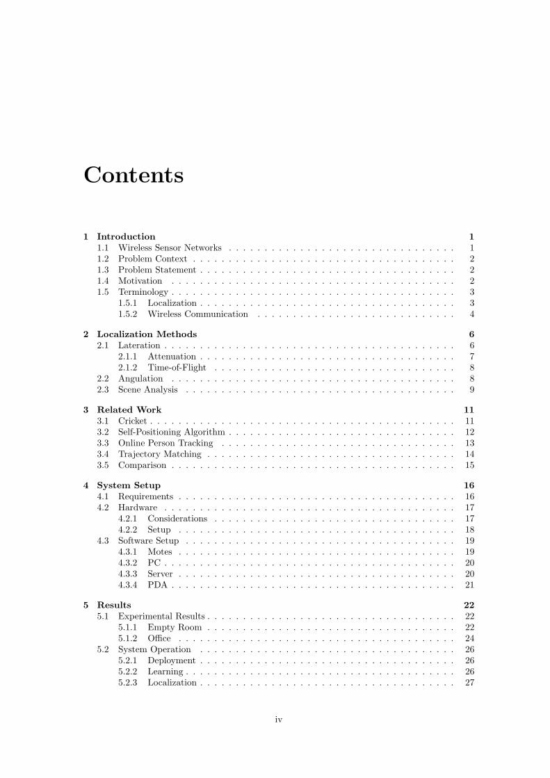
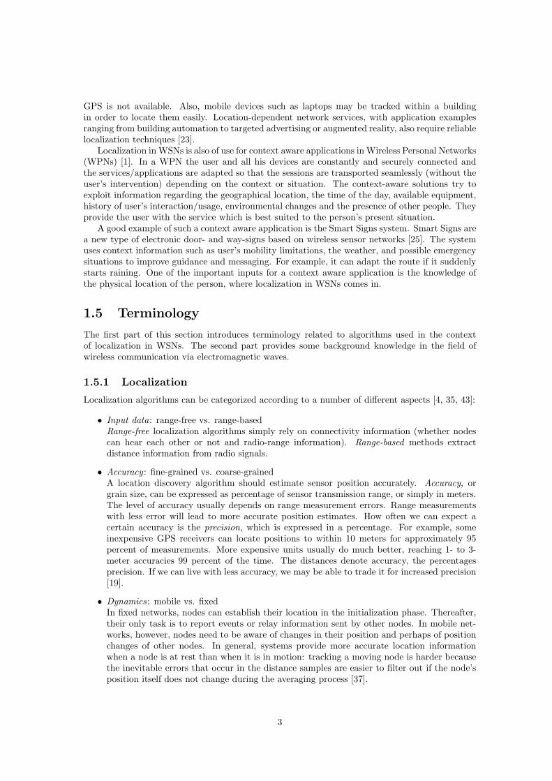
A Wireless Sensor Network (WSN) is a network of many small sensing and communicating devicescalled sensor nodes (or motes). Each node has a CPU, a power supply and a radio transceiver forcommunication. Interconnection between nodes is achieved via the transceiver. Typically, a WSNcontains one node, the base station, that connects the network to a more capable computer (Figure1.1), and probably to a network of general purpose computers through it. Sensors attached tothese nodes allow them to sense various phenomena within the environment. The typical purposeof a sensor network is to collect data via sensing interfaces and propagate those data to the centralcomputer, allowing easy monitoring of an environment.

Figure 1.1: Example of a Wireless Sensor Network.

Although a node is capable of dealing with a variety of jobs, it has many shortcomings aswell. The majority of the nodes currently available in the market are battery-operated, and hencethey have a limited life-time. Moreover, the memory capacity of a node is also limited. Life-time,processing and storage restrictions directly affect the algorithms designed for sensor networks. Asan example, a routing algorithm for WSNs must be energy and memory efficient. Since radiotransmissions consume a significant amount of energy, researchers generally seek ways to reduceradio communication as much as possible. However, when more information is stored and more

1

computation is done as to reduce the communication costs, energy consumption of the processorand memory components are becoming an important issue. Design choices have to be made, andthese also depend on the intended application.

1.2 Problem Context

Currently there is a prototype of a system available, developed within Logica’s Working Tomorrowprogram1, which uses motion sensors to secure an area [34] based on the Smart Dust concept. Theidea of the system is to monitor an area or room by a network of sensors with the size of adust particle. To be more precise, the Smart Dust project is ‘exploring whether an autonomoussensing, computing, and communication system can be packed into a cubic-millimeter mote (asmall particle or speck) to form the basis of integrated, massively distributed sensor networks’[42]. In the prototype the size of a sensor is significantly bigger than a dust particle. The momenta sensor detects movement in the area a message is sent to a central server. The server processesthe data and then uses Google Maps to produce a map which shows the detected movement. AGPS receiver is used to determine an absolute position, while RSSI (Received Signal StrengthIndicator) is used to locate the sensors relative to the GPS receiver. RSSI uses the decrease inenergy of the radio signal as it propagates in space to estimate the distance [7]. Experimentationwith the prototype system shows this method becomes unreliable when the batteries of the sensorsare getting weaker [34]. Simply using GPS receivers for all sensors is not an option as GPS cannotfunction in indoor and many outdoor applications, especially when there is no direct line of sightfrom nodes to terrestrial satellites. Besides, the use of these devices on sensor nodes is still achallenging issue due to their size, energy and price constraints [4]. As a result, there is a need forreliable localization in WSNs without the use of GPS receivers.

1.3 Problem Statement

The question which follows from the problem context is: How can we do localization in WSNswithout GPS? We will focus our research on algorithms suitable for mobile indoor networks.These algorithms will be compared with each other, based on a literature study. The goal isto develop a prototype in which localization is reliable and which can be used in a convincingdemonstration. For the purpose of a demonstration it is preferred that the deployment is ad-hoc and little configuration or calibration is required. The research questions reflect the twofoldapproach:

• Which systems and algorithms exist for reliable localization in mobile indoor wireless sensornetworks that use a minimal number of beacon nodes and how do they compare?

• Can we develop a prototype by implementing such an algorithm or an improvement thereofbased on an evaluation of algorithms?

1.4 Motivation

Usually, a Wireless Sensor Network is deployed to monitor its environment and for disaster responseand recovery systems. Applications include health monitoring systems, monitoring of wildlifehabitats [27] and nature reserves such as the Great Barrier Reef [21], and forest fire detectionsystems [11, 17, 24]. Examples of military applications are battlefield surveillance [5, 18] and thepreviously mentioned securing of an area or room.

Our focus, however, lies on localization in mobile indoor WSNs. Localization can be used fortracking objects or people. For example, our research may help people navigating indoors where

1Working Tomorrow is Logica’s graduate program that focuses on the feasibility and opportunities of innovativeICT solutions.

2

GPS is not available. Also, mobile devices such as laptops may be tracked within a buildingin order to locate them easily. Location-dependent network services, with application examplesranging from building automation to targeted advertising or augmented reality, also require reliablelocalization techniques [23].

Localization in WSNs is also of use for context aware applications in Wireless Personal Networks(WPNs) [1]. In a WPN the user and all his devices are constantly and securely connected andthe services/applications are adapted so that the sessions are transported seamlessly (without theuser’s intervention) depending on the context or situation. The context-aware solutions try toexploit information regarding the geographical location, the time of the day, available equipment,history of user’s interaction/usage, environmental changes and the presence of other people. Theyprovide the user with the service which is best suited to the person’s present situation.

A good example of such a context aware application is the Smart Signs system. Smart Signs area new type of electronic door- and way-signs based on wireless sensor networks [25]. The systemuses context information such as user’s mobility limitations, the weather, and possible emergencysituations to improve guidance and messaging. For example, it can adapt the route if it suddenlystarts raining. One of the important inputs for a context aware application is the knowledge ofthe physical location of the person, where localization in WSNs comes in.

1.5 Terminology

The first part of this section introduces terminology related to algorithms used in the contextof localization in WSNs. The second part provides some background knowledge in the field ofwireless communication via electromagnetic waves.

1.5.1 Localization

Localization algorithms can be categorized according to a number of different aspects [4, 35, 43]:

• Input data: range-free vs. range-basedRange-free localization algorithms simply rely on connectivity information (whether nodescan hear each other or not and radio-range information). Range-based methods extractdistance information from radio signals.

• Accuracy : fine-grained vs. coarse-grainedA location discovery algorithm should estimate sensor position accurately. Accuracy, orgrain size, can be expressed as percentage of sensor transmission range, or simply in meters.The level of accuracy usually depends on range measurement errors. Range measurementswith less error will lead to more accurate position estimates. How often we can expect acertain accuracy is the precision, which is expressed in a percentage. For example, someinexpensive GPS receivers can locate positions to within 10 meters for approximately 95percent of measurements. More expensive units usually do much better, reaching 1- to 3-meter accuracies 99 percent of the time. The distances denote accuracy, the percentagesprecision. If we can live with less accuracy, we may be able to trade it for increased precision[19].

• Dynamics: mobile vs. fixedIn fixed networks, nodes can establish their location in the initialization phase. Thereafter,their only task is to report events or relay information sent by other nodes. In mobile net-works, however, nodes need to be aware of changes in their position and perhaps of positionchanges of other nodes. In general, systems provide more accurate location informationwhen a node is at rest than when it is in motion: tracking a moving node is harder becausethe inevitable errors that occur in the distance samples are easier to filter out if the node’sposition itself does not change during the averaging process [37].

3

• Beacons: beacon-free vs. beacon-basedNodes with known positions are called beacon or anchor nodes. Beacon-based algorithmsusually produce an absolute location system where absolute positions of nodes are known, forexample, latitude, longitude, and altitude. However, the accuracy of the estimated positionis highly affected by the number of anchor nodes and their distribution in the sensor field.The ratio of beacon nodes to blind nodes (nodes with unknown positions) is generally quitesmall. The location of a beacon node can be determined using an attached GPS device orby manual deployment.

Beacon-free algorithms do not make any assumptions regarding node positions. In thiscase, instead of computing absolute node positions, relative positioning is used in which thecoordinate system is established by a reference group of nodes. Each object can also have itsown frame of reference [19]. For example, a mountain rescue team searching for avalanchevictims can use handheld computers to locate victims’ avalanche transceivers. Each rescuer’sdevice reports the victims’ positions relative to itself.

• Computational model : centralized vs. distributedIf an algorithm collects localization related data from the network and processes the datacollectively at a single station, then it is said to be centralized. If, on the other hand, eachnode collects partial data relevant to it and executes an algorithm to locate itself, thenthe localization algorithm is categorized as distributed. An intermediate form are so calledlocally centralized algorithms, which are distributed algorithms that achieve a global goal bycommunicating with nodes in some neighborhood only. For example, the sensor network canbe divided into local clusters, where each cluster has a head. All the range measurements ina certain cluster are forwarded to the cluster head, where computation takes place.

• Hops: single-hop vs. multi-hopA direct link between two neighbor nodes is called a hop. When the distance between twonodes is larger than the radio range but there are other nodes that create a continuous pathbetween them, the path is called a multi-hop path.

1.5.2 Wireless Communication

As sensor nodes use electromagnetic waves to communicate with each other we need to understandthe basics of how these waves propagate. Basic signal propagation and multipath propagation arediscussed.

Signal Propagation

A signal emitted by an antenna travels in the following three types of propagation modes: ground-wave propagation, sky-wave propagation, and line-of-sight (LOS) propagation. MW and LW radiois a kind of ground-wave propagation, where signals follow the contour of the Earth. Shortwaveradio is an example of sky-wave propagation, where radio signals are reflected by ionosphereand the ground along the way. Beyond 30 MHz, line-of-sight propagation dominates, meaningthat signal waves propagate on a direct, straight path in the air. Radio signals of line-of-sightpropagation can also penetrate objects, especially signals with frequencies just above 30 MHz [44].

Sensor motes support tunable frequencies in the range of 300 to 1000 MHz and the 2.4-GHzband. This means LOS propagation is dominant. The industrial, scientific and medical (ISM)radio bands were originally reserved internationally for the use of RF electromagnetic fields forindustrial, scientific and medical purposes other than communications. They have become a partof the radio spectrum that can be used by anybody without a license in most countries.

Multipath Propagation

For visible light we are well aware of the following effects: shadowing, reflection and refraction. Ingeneral, electromagnetic waves (including light) are also subject to diffraction and scattering [44].

4

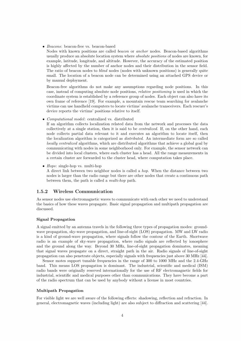
Radio communication is affected by the physical properties of waves; the combined effects maycause a transmitted radio signal to reach a receiver by two or more paths. This is called multipathpropagation and is illustrated in Figure 1.2.

• Shadowing and reflection occur when a signal encounters an object that is much larger thanits wavelength. Though the reflected signal and the shadowed signal are comparatively weak,they in effect help to propagate the signal to spaces where line-of-sight is impossible [44].Reflections occur from the surface of the earth and from buildings and walls.

• Refraction occurs when a wave passes across the boundary of two media [44]. Compare thisto how sunlight refracts when it enters water.

• Diffraction occurs at the edge of an impenetrable body that is large compared to the wave-length of the radio wave. When a radio wave encounters such an edge, waves propagatein different directions with the edge as the source [38]. Thus, signals can be received evenwhen there is no line-of-sight path between transmitter and receiver. For example, a wavecan ‘bend’ around a corner due to this effect.

• Scattering occurs when the medium through which the wave travels consists of objects withdimensions that are small compared to the wavelength, and where the number of obstaclesper unit volume is large. Scattered waves are produced by rough surfaces, small objects, orby other irregularities in the channel [36]. Typical objects that induce scattering are foliage,street signs, and lamp posts.

If there is line-of-sight between receiver and transmitter, then diffraction and scattering aregenerally minor effects, although reflection may have a significant impact. If there is no clear LOS,such as in an urban area at street level, then diffraction and scattering are the primary means ofsignal reception [38].

Figure 1.2: Multipath propagation: various effects give rise to additional radio propagation pathsbeyond the direct optical line-of-sight path between the transmitter and receiver. Image courtesyof Haas [16].

5

Chapter 2

Localization Methods

Triangulation, scene analysis, and proximity are the three principal techniques for automaticlocation-sensing [19]. Location systems may employ them individually or in combination. Thetriangulation location-sensing technique uses the geometric properties of triangles to computeobject locations. Triangulation is divisible into the subcategories of lateration, using distancemeasurements, and angulation, using primarily angle or bearing measurements. Scene analysisobserves features of its surroundings in order to determine the location of an object. In localizationbased on proximity, an object’s presence is sensed using a physical phenomenon with limited range,for example infrared or direct contact. We will cover lateration, angulation, and scene analysis inmore detail.

2.1 Lateration

Lateration computes the position of an object by measuring its distance from multiple referencepositions [19]. Calculating an object’s position in two dimensions requires distance measurementsfrom 3 points that do not all lie on a single line (non-collinear points). In three dimensions, distancemeasurements from 4 points not lying in the same plane (non-coplanar points) are required.Domain-specific knowledge may reduce the number of required distance measurements (e.g., inGPS, one computed position is in outer space).

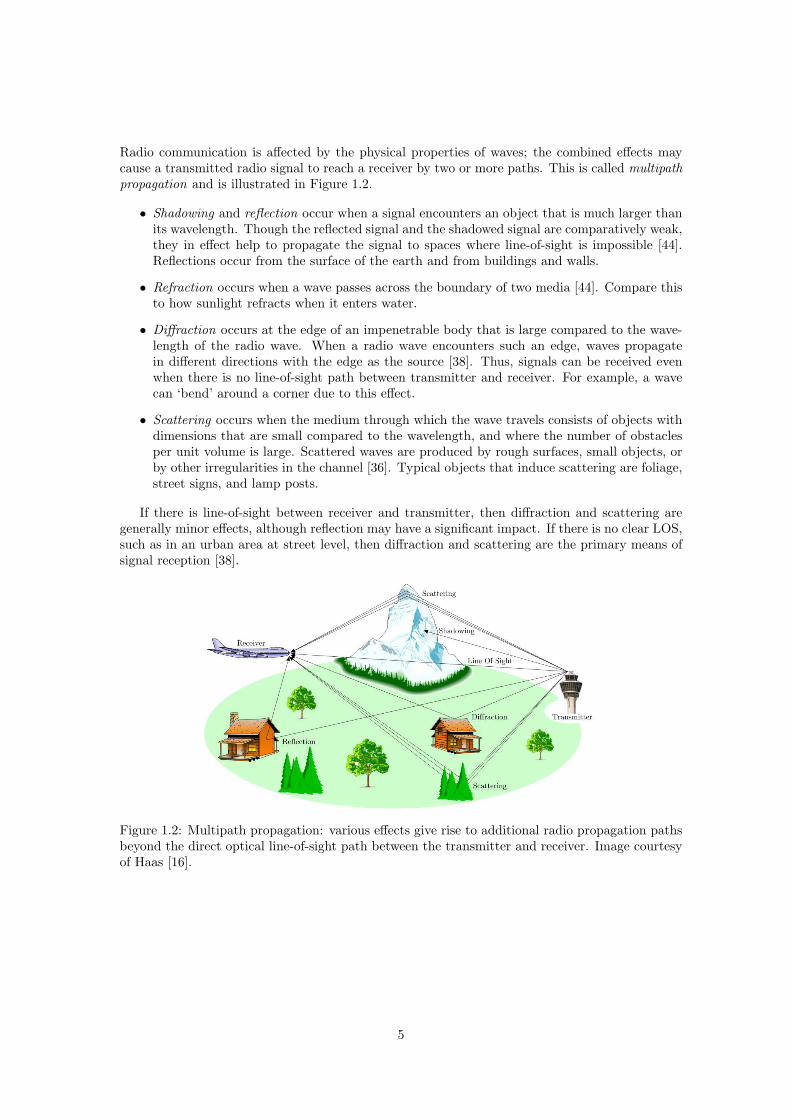
The 2D lateration technique works well when the three circles intersect at a single point, butthis is rarely the case when estimates are used in ranging. When the range of anchor nodes issufficiently large, the object to be located falls into a geometric region that is the intersection ofthree circles. This is called bounded intersection by Terwilliger [41] and is illustrated in Figure2.1a. It is also possible that the region of intersection is empty. This will occur if at least oneranging estimate is too small. Maximum likelihood methods overcome this problem by selectingthe point for localization that gives the minimum total error between measured estimates anddistances.

Lateration is quite expensive in the number of floating point operations that is required [22].A similar, but computationally less expensive solution is to use a bounding box approach. Themain idea is to construct a bounding box for each anchor using its position and distance estimate,and then to determine the intersection of these boxes. The position of the node is estimated tobe the center of the intersection box. Figure 2.1b illustrates the bounding box method for a nodewith distance estimates to three anchors. Note that, in this example, the estimated position bythe bounding box is close to the true position computed through lateration.

We will discuss two general approaches to measuring the distances (called ranging) requiredby the lateration technique, being attenuation and time-of-flight.

6

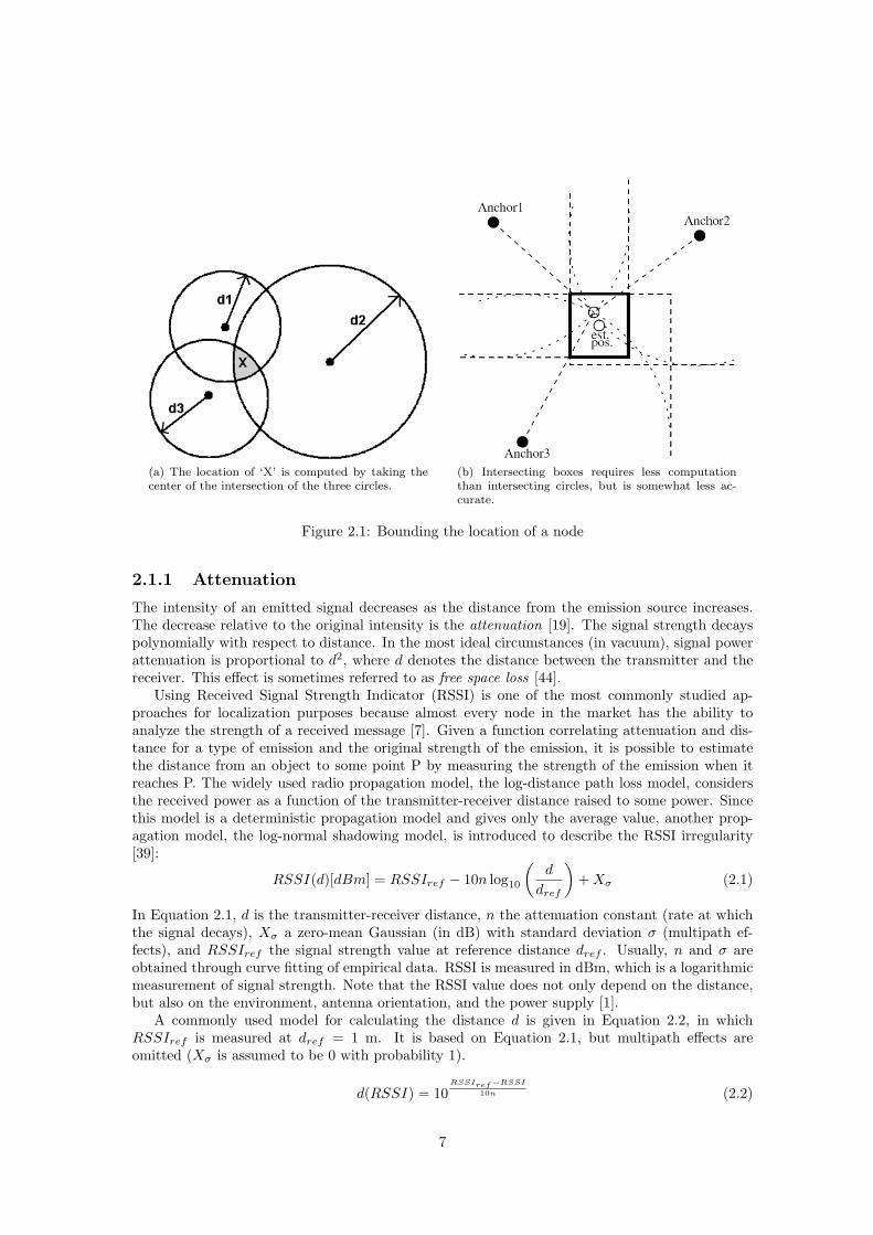
(a) The location of ‘X’ is computed by taking thecenter of the intersection of the three circles.

(b) Intersecting boxes requires less computationthan intersecting circles, but is somewhat less ac-curate.

Figure 2.1: Bounding the location of a node

2.1.1 Attenuation

The intensity of an emitted signal decreases as the distance from the emission source increases.The decrease relative to the original intensity is the attenuation [19]. The signal strength decayspolynomially with respect to distance. In the most ideal circumstances (in vacuum), signal powerattenuation is proportional to d2, where d denotes the distance between the transmitter and thereceiver. This effect is sometimes referred to as free space loss [44].

Using Received Signal Strength Indicator (RSSI) is one of the most commonly studied ap-proaches for localization purposes because almost every node in the market has the ability toanalyze the strength of a received message [7]. Given a function correlating attenuation and dis-tance for a type of emission and the original strength of the emission, it is possible to estimatethe distance from an object to some point P by measuring the strength of the emission when itreaches P. The widely used radio propagation model, the log-distance path loss model, considersthe received power as a function of the transmitter-receiver distance raised to some power. Sincethis model is a deterministic propagation model and gives only the average value, another prop-agation model, the log-normal shadowing model, is introduced to describe the RSSI irregularity[39]:

RSSI(d)[dBm] = RSSIref − 10n log10

(d

dref

)+Xσ (2.1)

In Equation 2.1, d is the transmitter-receiver distance, n the attenuation constant (rate at whichthe signal decays), Xσ a zero-mean Gaussian (in dB) with standard deviation σ (multipath ef-fects), and RSSIref the signal strength value at reference distance dref . Usually, n and σ areobtained through curve fitting of empirical data. RSSI is measured in dBm, which is a logarithmicmeasurement of signal strength. Note that the RSSI value does not only depend on the distance,but also on the environment, antenna orientation, and the power supply [1].

A commonly used model for calculating the distance d is given in Equation 2.2, in whichRSSIref is measured at dref = 1 m. It is based on Equation 2.1, but multipath effects areomitted (Xσ is assumed to be 0 with probability 1).

d(RSSI) = 10RSSIref−RSSI

10n (2.2)

7

In this scheme the attenuation constant is around 2 in an open-space environment, but its valueincreases if the environment is more complex (walls, large metallic objects, etc.). In environmentswith many obstructions such as an indoor office space, measuring distance using attenuation isusually less accurate than time-of-flight [19]. An approximation of the attenuation constant for anindoor environment is around 3.5 [36]. There is empirical evidence [12] that due to the unreliabilityof measurements, at best, accuracy in the scale of meters can be achieved regardless of the usedalgorithm or approach.

In the localization system Ferret, described by Terwilliger [41], two different ranging techniques(potentiometer and RSSI) are used to help locate an object to within one meter. In the poten-tiometer technique, the object to be located (a mobile node) begins by transmitting the beacon atthe lowest power level and listens for replies from the infrastructure nodes. Increasing the powerlevel with each transmission, once the mobile node gets three replies, it forwards its data to thebase station for position computation. A calibration tool needs to be run each time the system ismoved to a new environment in order to establish the communication ranges for given transmissionpower levels. Terwilliger also presents a location discovery algorithm that provides, for every nodein the network, a position estimate, as well as an associated error bound and confidence level.

2.1.2 Time-of-Flight

Measuring distance from an object to some point P using time-of-flight means measuring the timeit takes to travel between the object and point P at a known velocity. The object itself may bemoving, such as an airplane traveling at a known velocity for a given time interval, or, as is farmore typical, the object is approximately stationary and we are instead observing the differencein transmission and arrival time of an emitted signal [19]. GPS is a well-known system which usesthe time-of-flight technique.

There are two main issues in using time-of-flight. The first issue is to distinguish direct pulsesfrom reflected ones because they look identical. Reflected measurements may be pruned away byaggregating multiple receivers’ measurements and observing the environment’s reflective proper-ties. The second issue is agreement about the time. Since the propagation speed of radio signals isvery high (being equal to the speed of light), time measurements must be very accurate in order toavoid large uncertainties. For example, a localization accuracy of 1 meter requires timing accuracyon the level of 1

3∗108 ≈ 3.3 nanoseconds. This means a minimum clock rate of 300 MHz (3 ∗ 108

Hz) is required for hardware. As far as time synchronization goes, state-of-the-art protocols suchas FTSP [29] ‘only’ synchronize nodes in the order of microseconds. To avoid this issue, a nodecould reflect the radio signal back, but this once again requires constant delay for reflecting thesignal.

One can also measure the time difference of arrival. Cricket [33, 37], a location-support systemfor in-building, mobile, location-dependent applications, uses concurrent radio and ultrasoundsignals and measures the difference between the received times of the two types of signals. Assound waves travel at the speed of sound less precise timing than in the case of RF time-of-flightis required. A difference with radio signals is that an ultrasound signal does not go throughwalls; a similarity is that ultrasonic reception also suffers from severe multipath effects caused byreflections from walls and other objects. Cricket allows applications running on mobile and staticnodes to learn their physical location by using listeners that hear and analyze information frombeacons spread throughout a building. A case distinction is made for various situations in orderto overcome multipath and interference effects. Practical beacon configuration and positioningtechniques are used to improve accuracy up to the centimeter level.

2.2 Angulation

Angulation is similar to lateration except, instead of distances, angles are used for determining theposition of an object. This technique is also called angle-of-arrival. In general, two-dimensionalangulation requires two angle measurements and one length measurement such as the distance

8

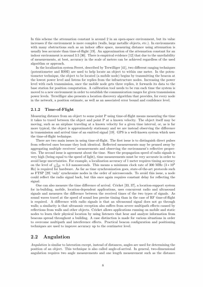
between the reference points as shown in Figure 2.2. In three dimensions, one length measurement,one azimuth measurement, and two angle measurements are needed to specify a precise position[19]. Although the definition of azimuth depends on the coordinate system, in this case, theazimuth is the horizontal component of an angle, measured around the horizon, from the northtoward the east. Angulation implementations sometimes choose to designate a constant referencevector (e.g., magnetic north) as 0◦.

All of the proposed solutions require special hardware (and are thus costly solutions). Ingeneral phased antenna arrays are used to measure the angle. Antenna arrays consist of multipleantennas with known separation in which each antenna measures the time of arrival of a signal.Given the differences in arrival times and the geometry of the receiving array, it is then possible tocompute the angle from which the emission originated. If there are enough elements in the arrayand large enough separations, the angulation calculation can be performed [19]. Other approachesdescribed in literature (see Basaran [4]) are compass sensors, rotating antennas, and rotating lightemitters combined with optical sensors.

Figure 2.2: This example of 2D angulation illustrateslocating object ‘X’ using angles relative to a 0◦ ref-erence vector and the distance between two referencepoints. 2D angulation always requires at least twoangle and one distance measurement to unambigu-ously locate an object [19].

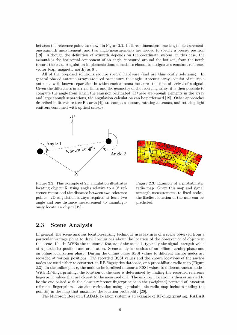
Figure 2.3: Example of a probabilisticradio map. Given this map and signalstrength measurements to fixed nodes,the likeliest location of the user can bepredicted.

2.3 Scene Analysis

In general, the scene analysis location-sensing technique uses features of a scene observed from aparticular vantage point to draw conclusions about the location of the observer or of objects inthe scene [19]. In WSNs the measured feature of the scene is typically the signal strength valueat a particular position and orientation. Scene analysis consists of an offline learning phase andan online localization phase. During the offline phase RSSI values to different anchor nodes arerecorded at various positions. The recorded RSSI values and the known locations of the anchornodes are used either to construct an RF-fingerprint database, or a probabilistic radio map (Figure2.3). In the online phase, the node to be localized measures RSSI values to different anchor nodes.With RF-fingerprinting, the location of the user is determined by finding the recorded referencefingerprint values that are closest to the measured one. The unknown location is then estimated tobe the one paired with the closest reference fingerprint or in the (weighted) centroid of k-nearestreference fingerprints. Location estimation using a probabilistic radio map includes finding thepoint(s) in the map that maximize the location probability [20].

The Microsoft Research RADAR location system is an example of RF-fingerprinting. RADAR

9

uses a dataset of signal strength measurements created by observing the radio transmissions of an802.11 wireless networking device at many positions and orientations throughout a building. Thelocation of other 802.11 network devices can then be computed by performing table lookup on theprebuilt dataset. The median resolution of RADAR is in the range of 2 to 3 meters [3].

MoteTrack [26] extends the approach and claims to be more robust than RADAR. Still, basestations at fixed locations are used and a form of fingerprinting is used for determining the locationof mobile nodes. However, the approach can tolerate the failure of up to 60% of the beacon nodeswithout severely degrading accuracy. Moreover, it is resilient to information loss, it can cope withperturbations in RF signals (which may be caused by changes in the environment, e.g., collapsedwalls in a disaster scenario), and is decentralized to prevent single point of failure.

Although fingerprinting can give accurate results, it is not appropriate for scenarios whereoffline calibration is infeasible (for example, if the area is hard to access). Furthermore, collectingall the RSSI samples is quite time-consuming.

10

Chapter 3

Related Work

This chapter is devoted to related work in mobile indoor localization. All the discussed approachesare range-based, because the accuracy of range-free algorithms is often limited by requiring densedeployments of sensor nodes [23].

3.1 Cricket

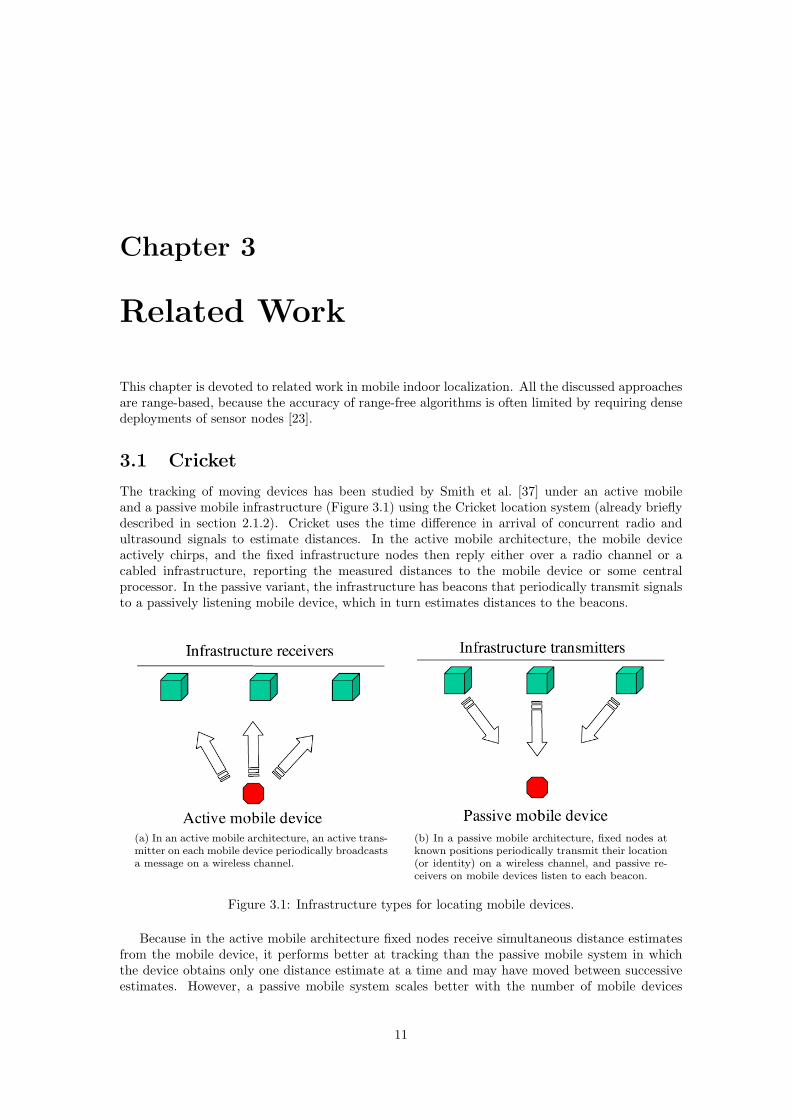
The tracking of moving devices has been studied by Smith et al. [37] under an active mobileand a passive mobile infrastructure (Figure 3.1) using the Cricket location system (already brieflydescribed in section 2.1.2). Cricket uses the time difference in arrival of concurrent radio andultrasound signals to estimate distances. In the active mobile architecture, the mobile deviceactively chirps, and the fixed infrastructure nodes then reply either over a radio channel or acabled infrastructure, reporting the measured distances to the mobile device or some centralprocessor. In the passive variant, the infrastructure has beacons that periodically transmit signalsto a passively listening mobile device, which in turn estimates distances to the beacons.

(a) In an active mobile architecture, an active trans-mitter on each mobile device periodically broadcastsa message on a wireless channel.

(b) In a passive mobile architecture, fixed nodes atknown positions periodically transmit their location(or identity) on a wireless channel, and passive re-ceivers on mobile devices listen to each beacon.

Figure 3.1: Infrastructure types for locating mobile devices.

Because in the active mobile architecture fixed nodes receive simultaneous distance estimatesfrom the mobile device, it performs better at tracking than the passive mobile system in whichthe device obtains only one distance estimate at a time and may have moved between successiveestimates. However, a passive mobile system scales better with the number of mobile devices

11

and puts users in control of whether their whereabouts are tracked. The authors devise a hybridapproach that tries to preserve the benefits of both approaches. During normal operation thepassive mobile system is used due to its scalability and guaranteed user-privacy. At start-up time,and when the system gets in a bad state and needs to be restarted, the listener transitions to activemobile operation to obtain multiple simultaneous beacon distance samples. In an experimentalsetup, a moving node was tracked in a single room. Six different speeds up to 1.43 m/s weretested. The accuracy is high in general but decreases somewhat as the speed increases.

Priyantha et al. [32] note it is almost impossible to deploy nodes in a typical office or home toachieve sufficient connectivity across all nearby nodes. For example, it is hard to obtain rangingbetween nodes placed inside and outside a room in a standard building. Due to the directionalityof the ultrasonic transmitters used, the ultrasonic-based ranging system has a 12 m range whenthe transmitter and the receiver are facing each other but less than 2 m mutual range when theyare on the same horizontal plane facing away from the plane (e.g., downwards from a ceiling).

3.2 Self-Positioning Algorithm

Capkun et al. introduce the Self-Positioning Algorithm (SPA) [6]. SPA defines and computesrelative positions of nodes in a mobile ad-hoc network without using GPS. It is a distributedalgorithm that does not use nodes with fixed or known positions. It assumes some method toestimate the distances between nodes and builds a relative coordinate system.

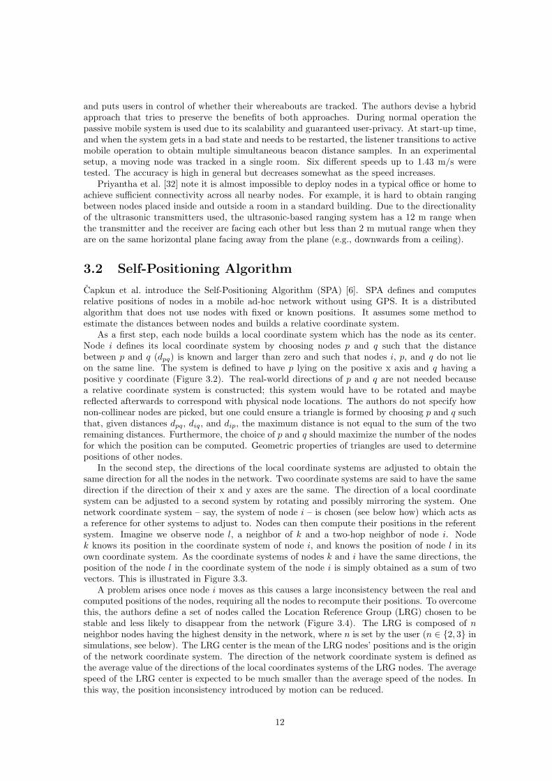
As a first step, each node builds a local coordinate system which has the node as its center.Node i defines its local coordinate system by choosing nodes p and q such that the distancebetween p and q (dpq) is known and larger than zero and such that nodes i, p, and q do not lieon the same line. The system is defined to have p lying on the positive x axis and q having apositive y coordinate (Figure 3.2). The real-world directions of p and q are not needed becausea relative coordinate system is constructed; this system would have to be rotated and maybereflected afterwards to correspond with physical node locations. The authors do not specify hownon-collinear nodes are picked, but one could ensure a triangle is formed by choosing p and q suchthat, given distances dpq, diq, and dip, the maximum distance is not equal to the sum of the tworemaining distances. Furthermore, the choice of p and q should maximize the number of the nodesfor which the position can be computed. Geometric properties of triangles are used to determinepositions of other nodes.

In the second step, the directions of the local coordinate systems are adjusted to obtain thesame direction for all the nodes in the network. Two coordinate systems are said to have the samedirection if the direction of their x and y axes are the same. The direction of a local coordinatesystem can be adjusted to a second system by rotating and possibly mirroring the system. Onenetwork coordinate system – say, the system of node i – is chosen (see below how) which acts asa reference for other systems to adjust to. Nodes can then compute their positions in the referentsystem. Imagine we observe node l, a neighbor of k and a two-hop neighbor of node i. Nodek knows its position in the coordinate system of node i, and knows the position of node l in itsown coordinate system. As the coordinate systems of nodes k and i have the same directions, theposition of the node l in the coordinate system of the node i is simply obtained as a sum of twovectors. This is illustrated in Figure 3.3.

A problem arises once node i moves as this causes a large inconsistency between the real andcomputed positions of the nodes, requiring all the nodes to recompute their positions. To overcomethis, the authors define a set of nodes called the Location Reference Group (LRG) chosen to bestable and less likely to disappear from the network (Figure 3.4). The LRG is composed of nneighbor nodes having the highest density in the network, where n is set by the user (n ∈ {2, 3} insimulations, see below). The LRG center is the mean of the LRG nodes’ positions and is the originof the network coordinate system. The direction of the network coordinate system is defined asthe average value of the directions of the local coordinates systems of the LRG nodes. The averagespeed of the LRG center is expected to be much smaller than the average speed of the nodes. Inthis way, the position inconsistency introduced by motion can be reduced.

12

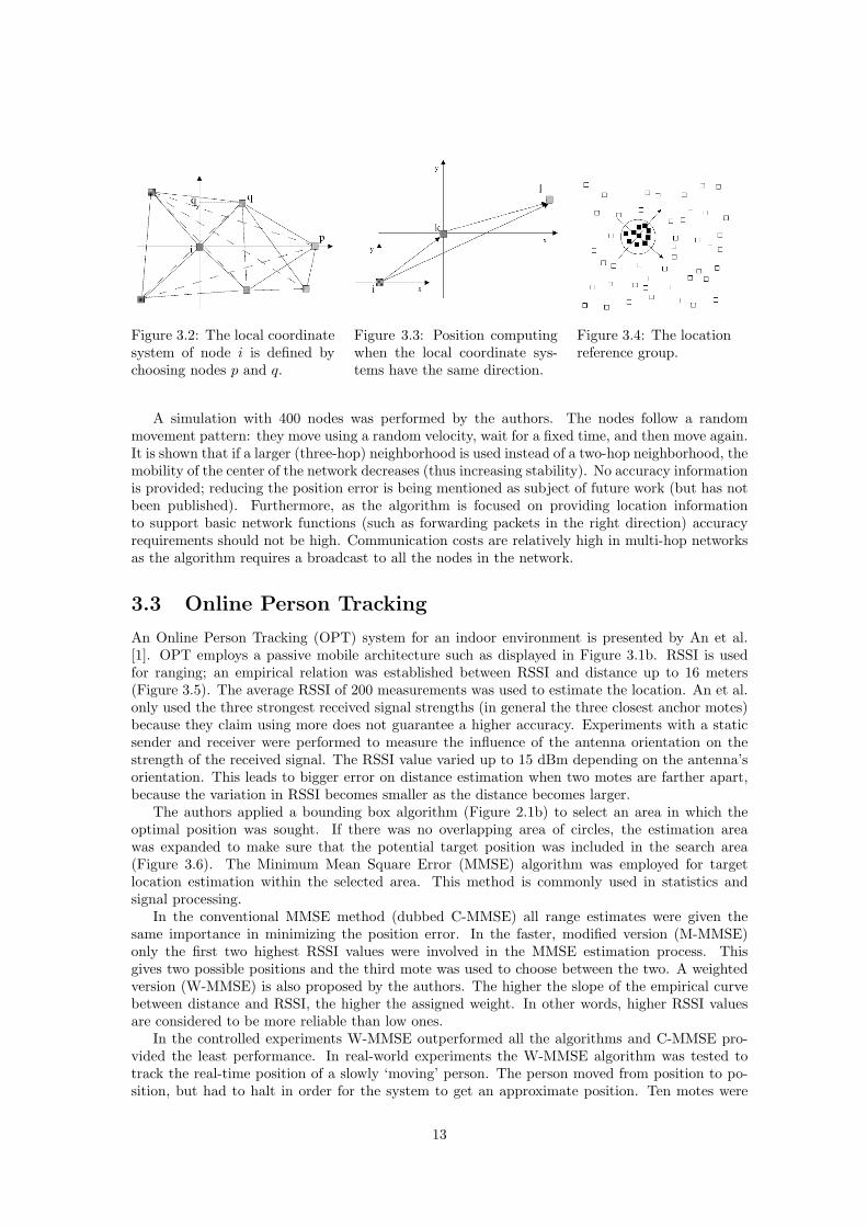
Figure 3.2: The local coordinatesystem of node i is defined bychoosing nodes p and q.

Figure 3.3: Position computingwhen the local coordinate sys-tems have the same direction.

Figure 3.4: The locationreference group.

A simulation with 400 nodes was performed by the authors. The nodes follow a randommovement pattern: they move using a random velocity, wait for a fixed time, and then move again.It is shown that if a larger (three-hop) neighborhood is used instead of a two-hop neighborhood, themobility of the center of the network decreases (thus increasing stability). No accuracy informationis provided; reducing the position error is being mentioned as subject of future work (but has notbeen published). Furthermore, as the algorithm is focused on providing location informationto support basic network functions (such as forwarding packets in the right direction) accuracyrequirements should not be high. Communication costs are relatively high in multi-hop networksas the algorithm requires a broadcast to all the nodes in the network.

3.3 Online Person Tracking

An Online Person Tracking (OPT) system for an indoor environment is presented by An et al.[1]. OPT employs a passive mobile architecture such as displayed in Figure 3.1b. RSSI is usedfor ranging; an empirical relation was established between RSSI and distance up to 16 meters(Figure 3.5). The average RSSI of 200 measurements was used to estimate the location. An et al.only used the three strongest received signal strengths (in general the three closest anchor motes)because they claim using more does not guarantee a higher accuracy. Experiments with a staticsender and receiver were performed to measure the influence of the antenna orientation on thestrength of the received signal. The RSSI value varied up to 15 dBm depending on the antenna’sorientation. This leads to bigger error on distance estimation when two motes are farther apart,because the variation in RSSI becomes smaller as the distance becomes larger.

The authors applied a bounding box algorithm (Figure 2.1b) to select an area in which theoptimal position was sought. If there was no overlapping area of circles, the estimation areawas expanded to make sure that the potential target position was included in the search area(Figure 3.6). The Minimum Mean Square Error (MMSE) algorithm was employed for targetlocation estimation within the selected area. This method is commonly used in statistics andsignal processing.

In the conventional MMSE method (dubbed C-MMSE) all range estimates were given thesame importance in minimizing the position error. In the faster, modified version (M-MMSE)only the first two highest RSSI values were involved in the MMSE estimation process. Thisgives two possible positions and the third mote was used to choose between the two. A weightedversion (W-MMSE) is also proposed by the authors. The higher the slope of the empirical curvebetween distance and RSSI, the higher the assigned weight. In other words, higher RSSI valuesare considered to be more reliable than low ones.

In the controlled experiments W-MMSE outperformed all the algorithms and C-MMSE pro-vided the least performance. In real-world experiments the W-MMSE algorithm was tested totrack the real-time position of a slowly ‘moving’ person. The person moved from position to po-sition, but had to halt in order for the system to get an approximate position. Ten motes were

13

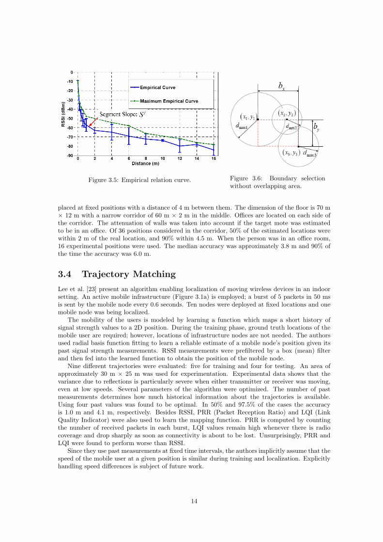
Figure 3.5: Empirical relation curve. Figure 3.6: Boundary selectionwithout overlapping area.

placed at fixed positions with a distance of 4 m between them. The dimension of the floor is 70 m× 12 m with a narrow corridor of 60 m × 2 m in the middle. Offices are located on each side ofthe corridor. The attenuation of walls was taken into account if the target mote was estimatedto be in an office. Of 36 positions considered in the corridor, 50% of the estimated locations werewithin 2 m of the real location, and 90% within 4.5 m. When the person was in an office room,16 experimental positions were used. The median accuracy was approximately 3.8 m and 90% ofthe time the accuracy was 6.0 m.

3.4 Trajectory Matching

Lee et al. [23] present an algorithm enabling localization of moving wireless devices in an indoorsetting. An active mobile infrastructure (Figure 3.1a) is employed; a burst of 5 packets in 50 msis sent by the mobile node every 0.6 seconds. Ten nodes were deployed at fixed locations and onemobile node was being localized.

The mobility of the users is modeled by learning a function which maps a short history ofsignal strength values to a 2D position. During the training phase, ground truth locations of themobile user are required; however, locations of infrastructure nodes are not needed. The authorsused radial basis function fitting to learn a reliable estimate of a mobile node’s position given itspast signal strength measurements. RSSI measurements were prefiltered by a box (mean) filterand then fed into the learned function to obtain the position of the mobile node.

Nine different trajectories were evaluated: five for training and four for testing. An area ofapproximately 30 m × 25 m was used for experimentation. Experimental data shows that thevariance due to reflections is particularly severe when either transmitter or receiver was moving,even at low speeds. Several parameters of the algorithm were optimized. The number of pastmeasurements determines how much historical information about the trajectories is available.Using four past values was found to be optimal. In 50% and 97.5% of the cases the accuracyis 1.0 m and 4.1 m, respectively. Besides RSSI, PRR (Packet Reception Ratio) and LQI (LinkQuality Indicator) were also used to learn the mapping function. PRR is computed by countingthe number of received packets in each burst, LQI values remain high whenever there is radiocoverage and drop sharply as soon as connectivity is about to be lost. Unsurprisingly, PRR andLQI were found to perform worse than RSSI.

Since they use past measurements at fixed time intervals, the authors implicitly assume that thespeed of the mobile user at a given position is similar during training and localization. Explicitlyhandling speed differences is subject of future work.

14

3.5 Comparison

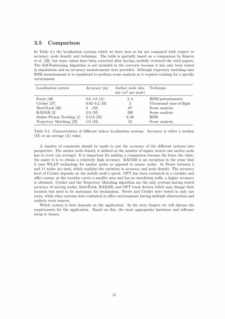
In Table 3.1 the localization systems which we have seen so far are compared with respect toaccuracy, node density and technique. The table is partially based on a comparison by Kasevaet al. [20], but some values have been corrected after having carefully reviewed the cited papers.The Self-Positioning Algorithm is not included in the overview because it has only been testedin simulations and no accuracy measurements were provided. Although trajectory matching usesRSSI measurements it is considered to perform scene analysis as it requires training for a specificenvironment.

Localization system Accuracy (m) Anchor node den-sity (m2 per node)

Technique

Ferret [40] 0.6–1.0 (A) 2–4 RSSI/potentiometerCricket [37] 0.02–0.2 (M) 2 Ultrasound time-of-flightMoteTrack [26] 2 (M) 87 Scene analysisRADAR [3] 2.9 (M) 326 Scene analysisOnline Person Tracking [1] 2/3.8 (M) 8/48 RSSITrajectory Matching [23] 1.0 (M) 52 Scene analysis

Table 3.1: Characteristics of different indoor localization systems. Accuracy is either a median(M) or an average (A) value.

A number of comments should be made to put the accuracy of the different systems intoperspective. The anchor node density is defined as the number of square meters one anchor nodehas to cover (on average). It is important for making a comparison because the lower the value,the easier it is to obtain a relatively high accuracy. RADAR is an exception in the sense thatit uses WLAN technology for anchor nodes as opposed to sensor nodes. In Ferret between 5and 11 nodes are used, which explains the variation in accuracy and node density. The accuracylevel of Cricket depends on the mobile node’s speed. OPT has been evaluated in a corridor andoffice rooms; as the corridor covers a smaller area and has no interfering walls, a higher accuracyis obtained. Cricket and the Trajectory Matching algorithm are the only systems having testedaccuracy of moving nodes; MoteTrack, RADAR, and OPT track devices which may change theirlocation but need to be stationary for localization. Ferret and Cricket were tested in only oneroom, while other systems were evaluated in office environments having multiple obstructions andrealistic error sources.

Which system is best depends on the application. In the next chapter we will discuss therequirements for the application. Based on this, the most appropriate hardware and softwaresetup is chosen.

15

Chapter 4

System Setup

The system setup depends on the intended application. Therefore, the requirements of the appli-cation are given first. Then, the considerations for the hardware choice are discussed, followed bythe hardware and software setup.

4.1 Requirements

The purpose of the application is to give a demonstration at a stand when Logica presents itselfat events (“Bedrijvenbeursdagen”). The primary goal is to show the relative positions of deployedsensor nodes on a map, which is displayed on a PDA. The secondary goal is to develop a devicewhich points the user to Logica’s stand and shows how far away it is located; for example, adisplay attached to a sensor node indicates the direction by an arrow and shows the distance inmeters.

The environment in which the WSN will operate and requirements with respect to accuracy,mobility, and deployment are described below. I have established these requirements in consulta-tion with my supervisor at Logica, Martijn Vlietstra, and verified them after writing them down.

Environment The events take place at various indoor locations which tend to be the sameevery year, although the location of the stand may change. The event floor is spacious andusually features pillars, but walls may also be present. Other obstructions include standsand (moving) people. Typically, the floor covers approximately 2500 m2 (50 m × 50 m). Allstands are located on the same level.

Accuracy The mean accuracy must be 5 meters or less. The maximum error allowed is 10 meters.

Mobility At least one node is mobile and its position needs to be updated as often as is needed toachieve the required accuracy. The maximum speed of the node is walking speed (1.4 m/s).

Deployment A number of static nodes will be deployed to help locate the mobile device(s).Deployment is done manually and must take no longer than 10 minutes. Preferably, staticnodes are to be placed at Logica’s stand, but other deployment locations are also possible.If the secondary goal is achieved, a second location can be used for handing out devices.

Availability The hardware should be commercially available; it will not be custom-built. Arange of RF motes and one ultrasound solution is currently available.

Cost A limited number of nodes can be bought.

16

4.2 Hardware

4.2.1 Considerations

The principal choice for a hardware solution is between an ultrasound (Cricket) and an RF-basedapproach, because this determines which localization methods are feasible. I will compare bothapproaches based on the requirements of the intended application. Per the availability requirement,we only consider off-the-shelf hardware.

Environment Both ultrasound and RF suffer from multipath effects caused by obstructions.Ultrasound is more limited, however, as the receiver and transmitter require line-of-sight.Furthermore, the range is fairly short: 12 meters in the most favorable case in the Cricketsystem. RF signals can be received up to at least 50 meters indoor [9], but this depends onthe hardware and environment. Because of their larger range, we decided that radio signalsare more suitable for the depicted environment.

Accuracy As far as accuracy is concerned, the use of either technique is plausible. Using ultra-sound can give accurate positions up to the centimeter level, but the requirements are notthat stringent. Radio-based approaches can also deliver the required accuracy (see section3.5), but this depends on the used algorithms and test setup. For example, if 10 nodesare used, the anchor node density will be 250 m2 per node, which leads to a much sparsernetwork (negatively influencing the accuracy) than is used in most of the discussed systems.

Mobility Both approaches can be used for tracking a mobile node. There are no specific advan-tages of either technique.

Deployment Limited time for deployment is available, so the system setup and calibration mustbe efficient. In Cricket careful orientation of the directional receiver is required, becausethe angle at which a signal is received is important for both accuracy and connectivity. RFmotes are less susceptible to erroneous placement as they have omnidirectional antennas ingeneral.

Interference The ultrasonic transmitter in Cricket operates at 40 kHz; it is found that somefluorescent lamps also generate 40 kHz ultrasonic waves which cause interference [30]. Otherthan this no interference is expected.

RF motes operate in the 868-MHz band or 2.4-GHz band. Not many devices operate in thefirst band, but in the second band WLAN is also present. Laptops and other devices at anevent are likely to use WLAN technology, and cannot be shut down.

Cost To cover the described area a dense network of Cricket motes would be required, whichwould lead to relatively high costs. The average RF mote costs two-thirds of one Cricketmote.

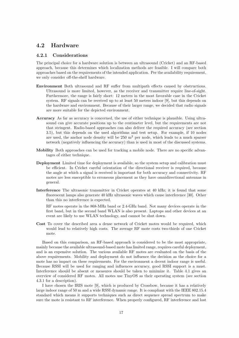
Based on this comparison, an RF-based approach is considered to be the most appropriate,mainly because the available ultrasound-based mote has limited range, requires careful deployment,and is an expensive solution. The various available RF motes are evaluated on the basis of theabove requirements. Mobility and deployment do not influence the decision as the choice for amote has no impact on these requirements. For the environment a decent indoor range is useful.Because RSSI will be used for ranging and influences accuracy, good RSSI support is a must.Interference should be absent or measures should be taken to minimize it. Table 4.1 gives anoverview of considered RF motes. All motes use TinyOS as their operating system (see section4.3.1 for a description).

I have chosen the IRIS mote [9], which is produced by Crossbow, because it has a relativelylarge indoor range of 50 m and a wide RSSI dynamic range. It is compliant with the IEEE 802.15.4standard which means it supports techniques such as direct sequence spread spectrum to makesure the mote is resistant to RF interference. When properly configured, RF interference and lost

17

RSSI

RF mote Frequency(MHz)

Maximum indoorrange (m)

dynamicrange (dBm)

accuracy(dB)

Cost (euro)

BTnode 868 ±30 −105 to −50 ±6 165IRIS 2405 ±50 −91 to −10 ±5 120Mica2 868 ±30 −105 to −50 ±6 120MicaZ 2405 ±30 −100 to 0 ±6 105TinyNode 184 868 ±50 −100 to −30 ±3 73TinyNode 584 868 ±100 −110 to −85 – 91

Table 4.1: Transceiver-related specifications and cost of considered RF motes.

data can be reduced through channel selection [8]. TinyNode 184 is also a good option, but is notchosen because driver support in TinyOS is limited for its transceiver at the time of writing.

The complete hardware setup is presented in the next section.

4.2.2 Setup

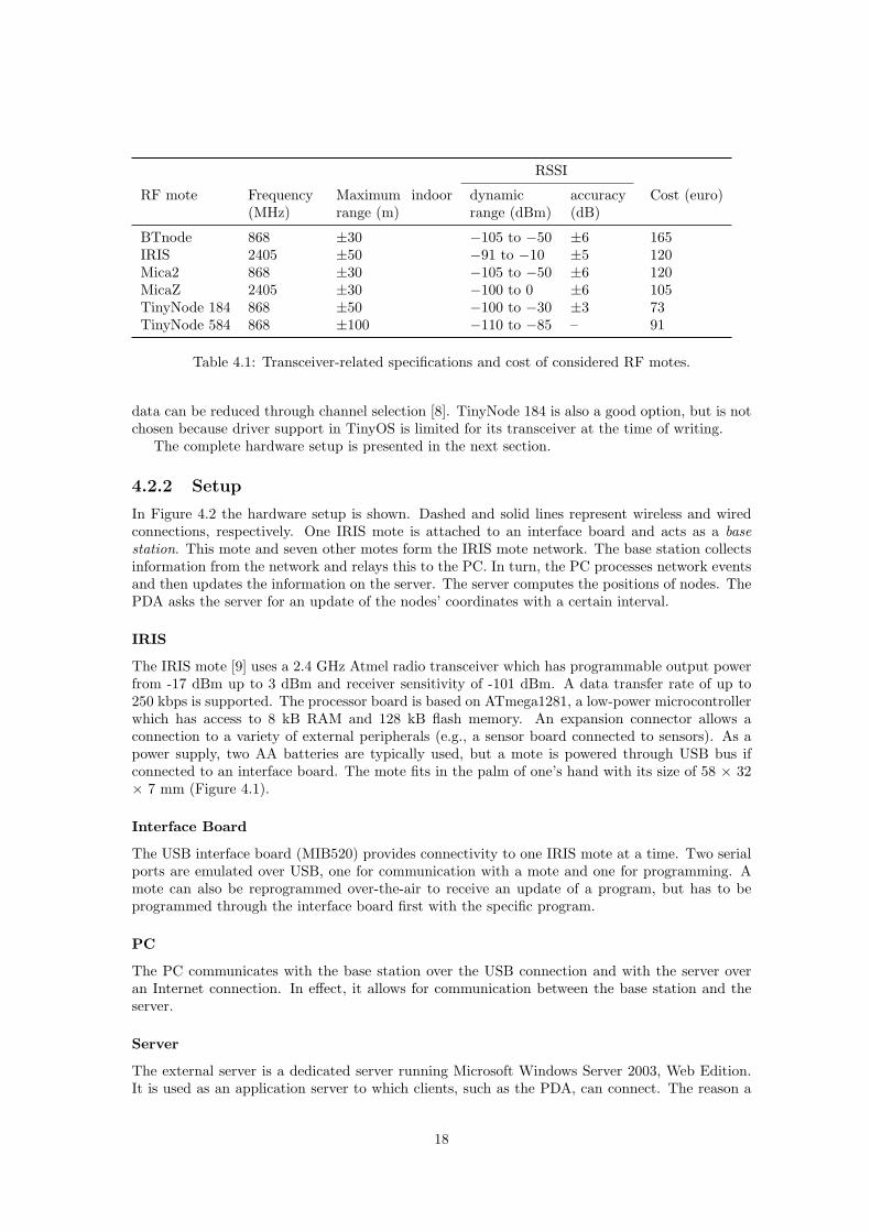
In Figure 4.2 the hardware setup is shown. Dashed and solid lines represent wireless and wiredconnections, respectively. One IRIS mote is attached to an interface board and acts as a basestation. This mote and seven other motes form the IRIS mote network. The base station collectsinformation from the network and relays this to the PC. In turn, the PC processes network eventsand then updates the information on the server. The server computes the positions of nodes. ThePDA asks the server for an update of the nodes’ coordinates with a certain interval.

IRIS

The IRIS mote [9] uses a 2.4 GHz Atmel radio transceiver which has programmable output powerfrom -17 dBm up to 3 dBm and receiver sensitivity of -101 dBm. A data transfer rate of up to250 kbps is supported. The processor board is based on ATmega1281, a low-power microcontrollerwhich has access to 8 kB RAM and 128 kB flash memory. An expansion connector allows aconnection to a variety of external peripherals (e.g., a sensor board connected to sensors). As apower supply, two AA batteries are typically used, but a mote is powered through USB bus ifconnected to an interface board. The mote fits in the palm of one’s hand with its size of 58 × 32× 7 mm (Figure 4.1).

Interface Board

The USB interface board (MIB520) provides connectivity to one IRIS mote at a time. Two serialports are emulated over USB, one for communication with a mote and one for programming. Amote can also be reprogrammed over-the-air to receive an update of a program, but has to beprogrammed through the interface board first with the specific program.

PC

The PC communicates with the base station over the USB connection and with the server overan Internet connection. In effect, it allows for communication between the base station and theserver.

Server

The external server is a dedicated server running Microsoft Windows Server 2003, Web Edition.It is used as an application server to which clients, such as the PDA, can connect. The reason a

18

server is used is because the PDA must be able to obtain the data from the PC over a wirelessconnection, which can be done relatively easy using this setup. Running the server application onthe PC would be possible, but connecting to it from outside the network the PC is in may provedifficult if the network is protected with a firewall.

PDA

The PDA is a HTC Advantage X7500 running Windows Mobile 5 at 624 MHz. It uses GPRS toconnect to the server. It is used to register the location of nodes in the deployment and learningphase (see section 5.2 for a description of the phases). This saves deployment time compared tousing a PC to connect to the server because the user does not have to keep walking back and forthto the PC between node registrations. In the localization phase, a mobile node and the PDA canbe used together to show the position of the PDA on the map, or the PDA can be used to trackanother person holding the mobile node. Note that the PDA is not connected to any sensor node.

Figure 4.1: IRIS mote Figure 4.2: Hardware setup

4.3 Software Setup

4.3.1 Motes

The way motes are programmed depends on their function. There are three types: base, static, andmobile. The base mote is connected to the interface board and has to handle the communicationbetween the PC and the mote network. All the non-mobile nodes listen for messages sent by mobilenodes. Each message contains the sender identification, packet number and sequence number. Themobile node sends a packet burst with a regular interval and increases the packet number by oneeach time this is done. The sequence number is used to identify a packet within a burst. RSSIand LQI information is requested for each packet by the receiver. All the data of one packet burstis aggregated into one message and then sent to the base station. The sending is done using amulti-hop routing protocol, because not every mote may be in range of the base station. I havewritten the software for the nodes, except the routing protocol. The motes use TinyOS.

TinyOS is an open-source, event-driven operating system designed for wireless embedded sensornetworks. It is written in nesC, which is an extension to the C programming language designedto embody the structuring concepts and execution model of TinyOS. Programs are built out ofcomponents, which are assembled to form whole programs. TinyOS’s component library includesnetwork protocols, distributed services, sensor drivers, and data acquisition tools.

There are two multi-hop routing protocols in TinyOS available: TYMO and the CollectionTree Protocol. TYMO is the implementation on TinyOS of the DYMO protocol, a point-to-pointrouting protocol for mobile ad-hoc networks. The current TYMO version is not stable, however.Therefore we have chosen to use the Collection Tree Protocol (CTP) [13, 14].

19

CTP is a tree-based collection protocol. Messages are collected at the roots of trees. Nodesform a set of routing trees to the tree roots. In our case, the only root is the base station. CTPis a best effort protocol: it does not promise 100% reliable delivery and there are no orderingguarantees. CTP assumes that it has link quality estimates of some number of nearby neighbors.As a link estimator we use an implementation of the four-bit wireless link estimation, which canmaintain a 99% delivery ratio with a transmission power of 0 dBm over large, multi-hop testbeds[15].

CTP works as follows. Nodes generate routes to roots using a routing gradient (informationused to decide how to route). The protocol uses the expected number of transmissions (ETX)as its routing gradient (the lower the value, the better the link). CTP represents ETX values as16-bit fixed-point real numbers with a precision of hundredths. A root has an ETX of 0. TheETX of a node is the ETX of its parent plus the ETX of its link to its parent. In general, CTPchooses the node with the lowest ETX value, unless it has reasons to do otherwise (e.g., afterlosing connectivity with a candidate parent). CTP data frames also have a time has lived (THL)field, which the routing layer increments on each hop. CTP uses the ETX and THL fields to dealwith routing loops and packet duplication.

4.3.2 PC

The PC connects to the server as a client and forwards messages it has received from the basestation. TinyOS provides classes to read and interpret data sent over the USB port. I have writtena Java program which sets up the connection to the server. Furthermore, it drops duplicate packetsand then sends the unique ones to the server.

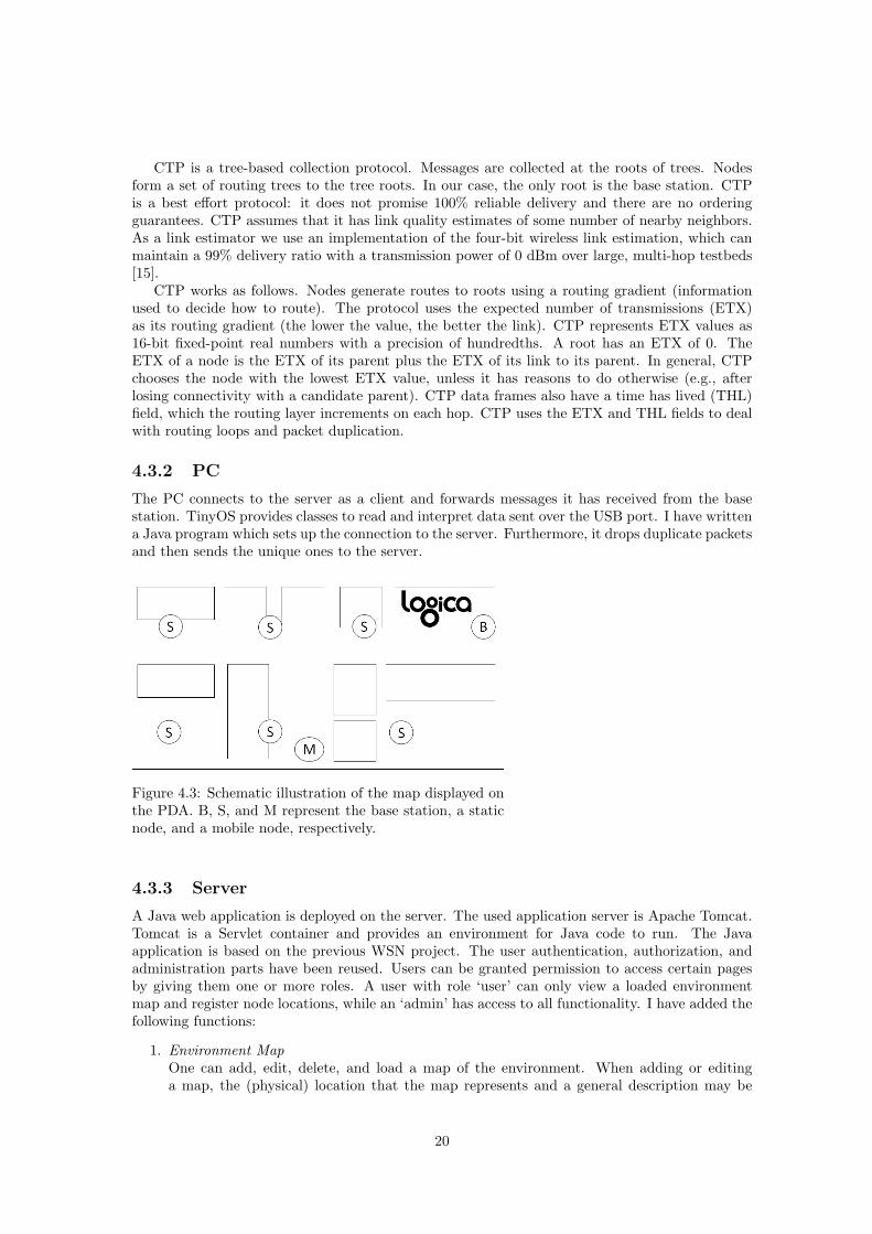
Figure 4.3: Schematic illustration of the map displayed onthe PDA. B, S, and M represent the base station, a staticnode, and a mobile node, respectively.

4.3.3 Server

A Java web application is deployed on the server. The used application server is Apache Tomcat.Tomcat is a Servlet container and provides an environment for Java code to run. The Javaapplication is based on the previous WSN project. The user authentication, authorization, andadministration parts have been reused. Users can be granted permission to access certain pagesby giving them one or more roles. A user with role ‘user’ can only view a loaded environmentmap and register node locations, while an ‘admin’ has access to all functionality. I have added thefollowing functions:

1. Environment MapOne can add, edit, delete, and load a map of the environment. When adding or editinga map, the (physical) location that the map represents and a general description may be

20

specified. The name and image file location must be specified. The width and height thatthe map represents in the physical world are also required. When a map is loaded the imageis displayed. A schematic example of what could be displayed is shown in Figure 4.3. Theposition of the mobile node is updated regularly.

2. Node RegistrationIf a map has been loaded, the user can enter the location of a static node on the map byclicking on it and entering the node number. These locations are saved and displayed. Whenthe map is reloaded or another map is loaded, the nodes and their positions are deleted.

4.3.4 PDA

The PDA uses Opera Mobile 9.5 as a browser to view the Java web application. This browser isused because of its good support of web standards on a mobile device.

21

Chapter 5

Results

5.1 Experimental Results

To determine the relation between signal strength and distance we need to perform measurements.I used two motes: a sending mote and a base station for receiving the messages and transferringthem to a laptop. The base station collects three values: RSSI, LQI, and PRR. RSSI is explainedin section 2.1.1 and is a value between −91 and −10 dBm. LQI stands for Link Quality Indication.The IEEE 802.15.4 standard defines the LQI measurement as a characterization of the strengthand/or quality of a received packet. LQI values are integers ranging from 0 to 255 (the higherthe value, the better the link) [2]. PRR is the Packet Reception Rate and is the ratio of receivedpackets to the total number of packets. RSSI and LQI are provided by the mote’s transceiver;PRR is computed. No WiFi networks were present which could interfere.

A series of parameters influence the RSSI measurements. We describe the ones identified byStoyanova et al. [39]:

RF frequency A center frequency of 2.405 GHz (channel 11) is used. Note that channels 11,25, and 26 are suited to avoid interference with WiFi [8]. Channel 11 has been found to bethe most reliable channel for the IRIS mote’s transceiver by TinyOS developers. The centerfrequency FCH is defined as follows: FCH = 2405 + 5× (channel − 11)[MHz] [2].

Antenna orientation Both motes were in a horizontal position. The sending mote was alwaysin front of the person holding it. This means the person was an obstruction in case of thesender moving away from the receiver.

Variation of transceivers The same motes were used each time for the sender and base station.

Transmission power The transmission power is set to the maximum output power of the IRISmote, being 3.0 dBm, unless noted otherwise.

Environment We conducted the first set of experiments in an empty room of 50 m × 16 m,measuring 2.7 m in height. The second set was measured in an open workspace environmentof the same size (illustrated in Figure 5.1 and 5.2), the only difference being five extra officerooms located farthest away from the base station.

Height from the ground The base station was placed on a chair at a height of 0.58 m. Thesending mote was held 1.0–1.1 m above the ground.

5.1.1 Empty Room

I performed two experiments in the empty room. The sending mote was static in the first experi-ment and moving in the second. The transmitter sends a packet burst of five messages as fast aspossible (in general within 50 ms). PRR is computed per packet burst.

22

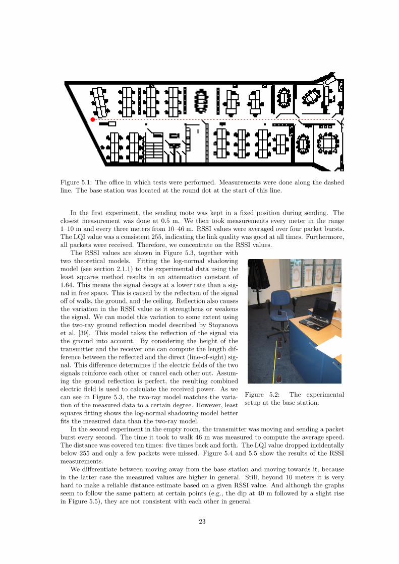
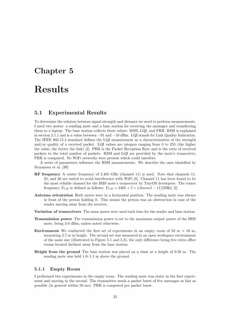
Figure 5.1: The office in which tests were performed. Measurements were done along the dashedline. The base station was located at the round dot at the start of this line.

In the first experiment, the sending mote was kept in a fixed position during sending. Theclosest measurement was done at 0.5 m. We then took measurements every meter in the range1–10 m and every three meters from 10–46 m. RSSI values were averaged over four packet bursts.The LQI value was a consistent 255, indicating the link quality was good at all times. Furthermore,all packets were received. Therefore, we concentrate on the RSSI values.

Figure 5.2: The experimentalsetup at the base station.

The RSSI values are shown in Figure 5.3, together withtwo theoretical models. Fitting the log-normal shadowingmodel (see section 2.1.1) to the experimental data using theleast squares method results in an attenuation constant of1.64. This means the signal decays at a lower rate than a sig-nal in free space. This is caused by the reflection of the signaloff of walls, the ground, and the ceiling. Reflection also causesthe variation in the RSSI value as it strengthens or weakensthe signal. We can model this variation to some extent usingthe two-ray ground reflection model described by Stoyanovaet al. [39]. This model takes the reflection of the signal viathe ground into account. By considering the height of thetransmitter and the receiver one can compute the length dif-ference between the reflected and the direct (line-of-sight) sig-nal. This difference determines if the electric fields of the twosignals reinforce each other or cancel each other out. Assum-ing the ground reflection is perfect, the resulting combinedelectric field is used to calculate the received power. As wecan see in Figure 5.3, the two-ray model matches the varia-tion of the measured data to a certain degree. However, leastsquares fitting shows the log-normal shadowing model betterfits the measured data than the two-ray model.

In the second experiment in the empty room, the transmitter was moving and sending a packetburst every second. The time it took to walk 46 m was measured to compute the average speed.The distance was covered ten times: five times back and forth. The LQI value dropped incidentallybelow 255 and only a few packets were missed. Figure 5.4 and 5.5 show the results of the RSSImeasurements.

We differentiate between moving away from the base station and moving towards it, becausein the latter case the measured values are higher in general. Still, beyond 10 meters it is veryhard to make a reliable distance estimate based on a given RSSI value. And although the graphsseem to follow the same pattern at certain points (e.g., the dip at 40 m followed by a slight risein Figure 5.5), they are not consistent with each other in general.

23

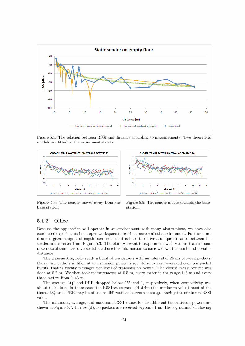
Figure 5.3: The relation between RSSI and distance according to measurements. Two theoreticalmodels are fitted to the experimental data.

Figure 5.4: The sender moves away from thebase station.

Figure 5.5: The sender moves towards the basestation.

5.1.2 Office

Because the application will operate in an environment with many obstructions, we have alsoconducted experiments in an open workspace to test in a more realistic environment. Furthermore,if one is given a signal strength measurement it is hard to derive a unique distance between thesender and receiver from Figure 5.3. Therefore we want to experiment with various transmissionpowers to obtain more diverse data and use this information to narrow down the number of possibledistances.

The transmitting node sends a burst of ten packets with an interval of 25 ms between packets.Every two packets a different transmission power is set. Results were averaged over ten packetbursts, that is twenty messages per level of transmission power. The closest measurement wasdone at 0.2 m. We then took measurements at 0.5 m, every meter in the range 1–3 m and everythree meters from 3–43 m.

The average LQI and PRR dropped below 255 and 1, respectively, when connectivity wasabout to be lost. In these cases the RSSI value was −91 dBm (the minimum value) most of thetimes. LQI and PRR may be of use to differentiate between messages having the minimum RSSIvalue.

The minimum, average, and maximum RSSI values for the different transmission powers areshown in Figure 5.7. In case (d), no packets are received beyond 31 m. The log-normal shadowing

24

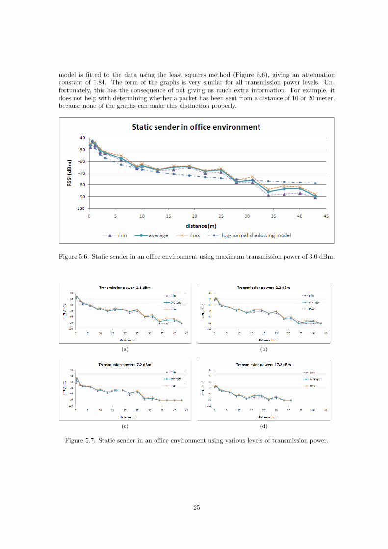
model is fitted to the data using the least squares method (Figure 5.6), giving an attenuationconstant of 1.84. The form of the graphs is very similar for all transmission power levels. Un-fortunately, this has the consequence of not giving us much extra information. For example, itdoes not help with determining whether a packet has been sent from a distance of 10 or 20 meter,because none of the graphs can make this distinction properly.

Figure 5.6: Static sender in an office environment using maximum transmission power of 3.0 dBm.

(a) (b)

(c) (d)

Figure 5.7: Static sender in an office environment using various levels of transmission power.

25

5.2 System Operation

There are three phases in the system’s operation: deployment, learning, and localization.

5.2.1 Deployment

First, the user loads a map of the current environment through the server’s web interface. He or shethen deploys nodes manually and registers their approximate positions (except for mobile nodes).To save deployment time it would be better if node positions are determined automatically, butto do this the WSN has to have two properties: global rigidity and a rather high node degree.

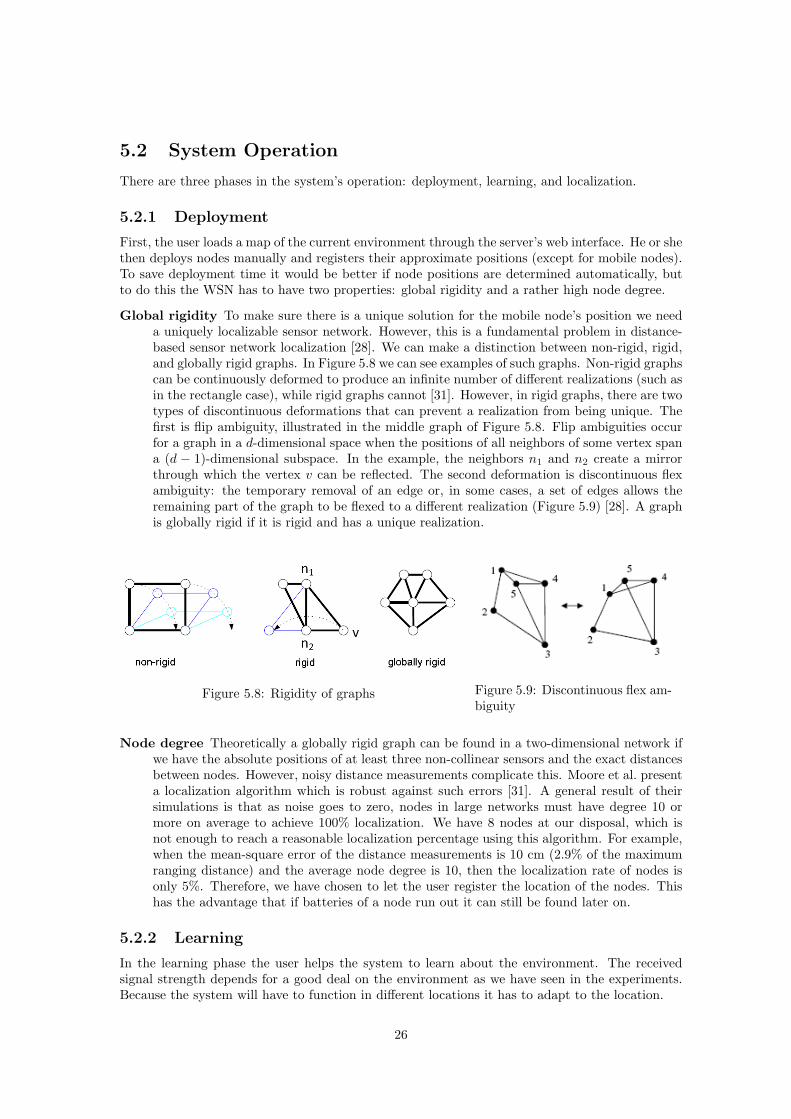
Global rigidity To make sure there is a unique solution for the mobile node’s position we needa uniquely localizable sensor network. However, this is a fundamental problem in distance-based sensor network localization [28]. We can make a distinction between non-rigid, rigid,and globally rigid graphs. In Figure 5.8 we can see examples of such graphs. Non-rigid graphscan be continuously deformed to produce an infinite number of different realizations (such asin the rectangle case), while rigid graphs cannot [31]. However, in rigid graphs, there are twotypes of discontinuous deformations that can prevent a realization from being unique. Thefirst is flip ambiguity, illustrated in the middle graph of Figure 5.8. Flip ambiguities occurfor a graph in a d-dimensional space when the positions of all neighbors of some vertex spana (d − 1)-dimensional subspace. In the example, the neighbors n1 and n2 create a mirrorthrough which the vertex v can be reflected. The second deformation is discontinuous flexambiguity: the temporary removal of an edge or, in some cases, a set of edges allows theremaining part of the graph to be flexed to a different realization (Figure 5.9) [28]. A graphis globally rigid if it is rigid and has a unique realization.

Figure 5.8: Rigidity of graphs Figure 5.9: Discontinuous flex am-biguity

Node degree Theoretically a globally rigid graph can be found in a two-dimensional network ifwe have the absolute positions of at least three non-collinear sensors and the exact distancesbetween nodes. However, noisy distance measurements complicate this. Moore et al. presenta localization algorithm which is robust against such errors [31]. A general result of theirsimulations is that as noise goes to zero, nodes in large networks must have degree 10 ormore on average to achieve 100% localization. We have 8 nodes at our disposal, which isnot enough to reach a reasonable localization percentage using this algorithm. For example,when the mean-square error of the distance measurements is 10 cm (2.9% of the maximumranging distance) and the average node degree is 10, then the localization rate of nodes isonly 5%. Therefore, we have chosen to let the user register the location of the nodes. Thishas the advantage that if batteries of a node run out it can still be found later on.

5.2.2 Learning

In the learning phase the user helps the system to learn about the environment. The receivedsignal strength depends for a good deal on the environment as we have seen in the experiments.Because the system will have to function in different locations it has to adapt to the location.

26

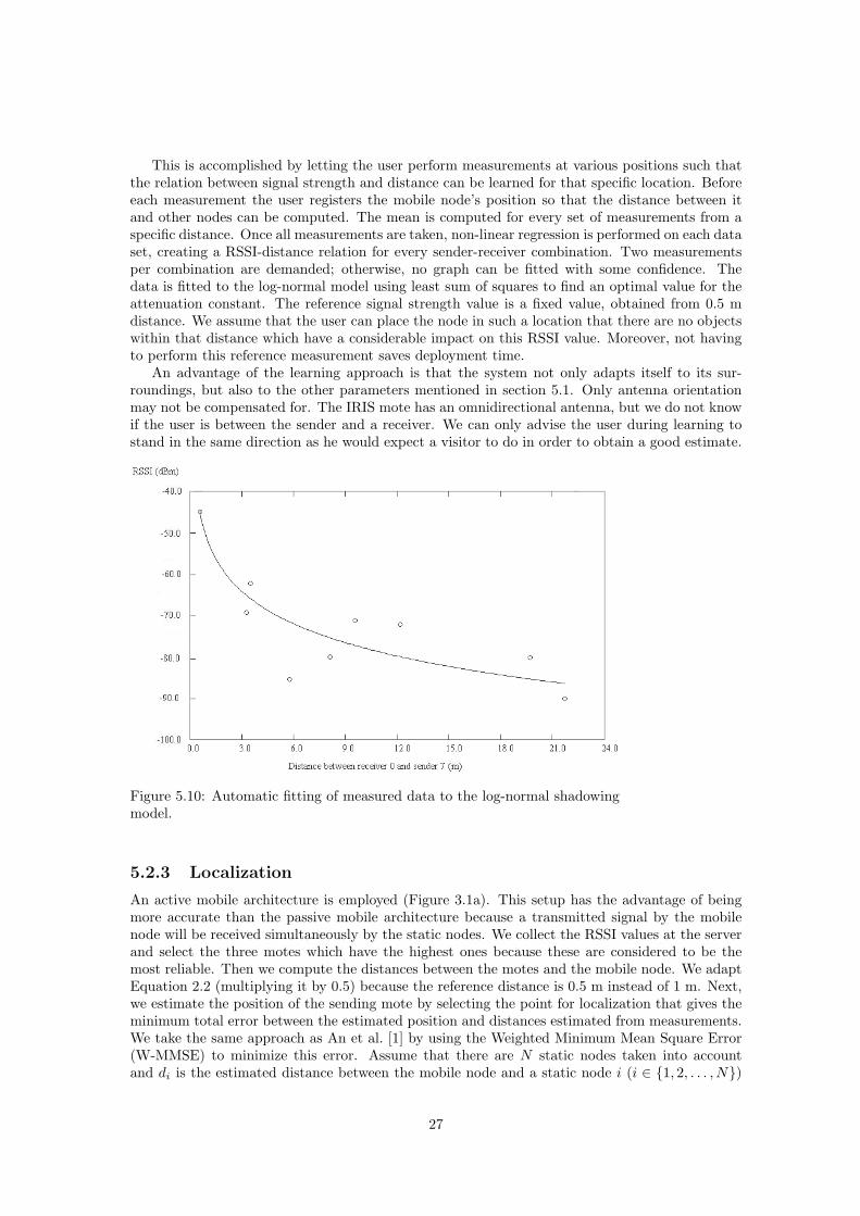
This is accomplished by letting the user perform measurements at various positions such thatthe relation between signal strength and distance can be learned for that specific location. Beforeeach measurement the user registers the mobile node’s position so that the distance between itand other nodes can be computed. The mean is computed for every set of measurements from aspecific distance. Once all measurements are taken, non-linear regression is performed on each dataset, creating a RSSI-distance relation for every sender-receiver combination. Two measurementsper combination are demanded; otherwise, no graph can be fitted with some confidence. Thedata is fitted to the log-normal model using least sum of squares to find an optimal value for theattenuation constant. The reference signal strength value is a fixed value, obtained from 0.5 mdistance. We assume that the user can place the node in such a location that there are no objectswithin that distance which have a considerable impact on this RSSI value. Moreover, not havingto perform this reference measurement saves deployment time.

An advantage of the learning approach is that the system not only adapts itself to its sur-roundings, but also to the other parameters mentioned in section 5.1. Only antenna orientationmay not be compensated for. The IRIS mote has an omnidirectional antenna, but we do not knowif the user is between the sender and a receiver. We can only advise the user during learning tostand in the same direction as he would expect a visitor to do in order to obtain a good estimate.

Figure 5.10: Automatic fitting of measured data to the log-normal shadowingmodel.

5.2.3 Localization

An active mobile architecture is employed (Figure 3.1a). This setup has the advantage of beingmore accurate than the passive mobile architecture because a transmitted signal by the mobilenode will be received simultaneously by the static nodes. We collect the RSSI values at the serverand select the three motes which have the highest ones because these are considered to be themost reliable. Then we compute the distances between the motes and the mobile node. We adaptEquation 2.2 (multiplying it by 0.5) because the reference distance is 0.5 m instead of 1 m. Next,we estimate the position of the sending mote by selecting the point for localization that gives theminimum total error between the estimated position and distances estimated from measurements.We take the same approach as An et al. [1] by using the Weighted Minimum Mean Square Error(W-MMSE) to minimize this error. Assume that there are N static nodes taken into accountand di is the estimated distance between the mobile node and a static node i (i ∈ {1, 2, . . . , N})

27

located at (xi, yi), then we can define the error estimation function as:

MMSE =

√√√√ n∑i=1

wi · error2i (5.1)

where wi = 1di

, errori = |di −√

(xi − xe)2 + (yi − ye)2| and (xe, ye) is the estimated position intwo-dimensional coordinates of the mobile node.

5.3 System Validation

This section validates whether the built system meets explicit and implicit requirements. Theexplicit requirements are described in section 4.1, while the implicit ones were, as by definition,not written down.

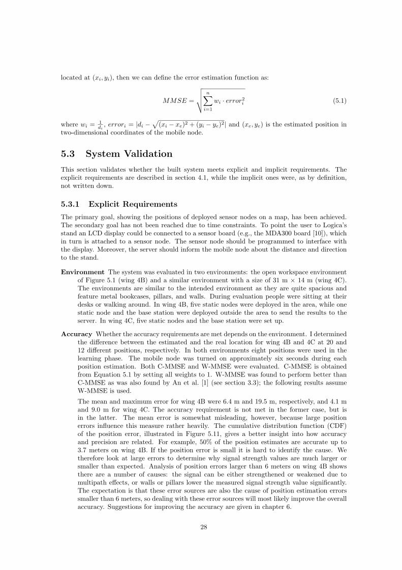
5.3.1 Explicit Requirements

The primary goal, showing the positions of deployed sensor nodes on a map, has been achieved.The secondary goal has not been reached due to time constraints. To point the user to Logica’sstand an LCD display could be connected to a sensor board (e.g., the MDA300 board [10]), whichin turn is attached to a sensor node. The sensor node should be programmed to interface withthe display. Moreover, the server should inform the mobile node about the distance and directionto the stand.

Environment The system was evaluated in two environments: the open workspace environmentof Figure 5.1 (wing 4B) and a similar environment with a size of 31 m × 14 m (wing 4C).The environments are similar to the intended environment as they are quite spacious andfeature metal bookcases, pillars, and walls. During evaluation people were sitting at theirdesks or walking around. In wing 4B, five static nodes were deployed in the area, while onestatic node and the base station were deployed outside the area to send the results to theserver. In wing 4C, five static nodes and the base station were set up.

Accuracy Whether the accuracy requirements are met depends on the environment. I determinedthe difference between the estimated and the real location for wing 4B and 4C at 20 and12 different positions, respectively. In both environments eight positions were used in thelearning phase. The mobile node was turned on approximately six seconds during eachposition estimation. Both C-MMSE and W-MMSE were evaluated. C-MMSE is obtainedfrom Equation 5.1 by setting all weights to 1. W-MMSE was found to perform better thanC-MMSE as was also found by An et al. [1] (see section 3.3); the following results assumeW-MMSE is used.

The mean and maximum error for wing 4B were 6.4 m and 19.5 m, respectively, and 4.1 mand 9.0 m for wing 4C. The accuracy requirement is not met in the former case, but isin the latter. The mean error is somewhat misleading, however, because large positionerrors influence this measure rather heavily. The cumulative distribution function (CDF)of the position error, illustrated in Figure 5.11, gives a better insight into how accuracyand precision are related. For example, 50% of the position estimates are accurate up to3.7 meters on wing 4B. If the position error is small it is hard to identify the cause. Wetherefore look at large errors to determine why signal strength values are much larger orsmaller than expected. Analysis of position errors larger than 6 meters on wing 4B showsthere are a number of causes: the signal can be either strengthened or weakened due tomultipath effects, or walls or pillars lower the measured signal strength value significantly.The expectation is that these error sources are also the cause of position estimation errorssmaller than 6 meters, so dealing with these error sources will most likely improve the overallaccuracy. Suggestions for improving the accuracy are given in chapter 6.

28

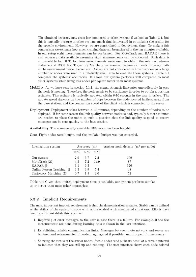
The obtained accuracy may seem low compared to other systems if we look at Table 3.1, butthis is partially because in other systems much time is invested in optimizing the results forthe specific environment. However, we are constrained in deployment time. To make a faircomparison we estimate how much training data can be gathered in the ten minutes available.In our setup eight measurements can be performed. For MoteTrack and RADAR there isalso accuracy data available assuming eight measurements can be collected. Such data isnot available for OPT; fourteen measurements were used to obtain the relation betweendistance and RSSI. For Trajectory Matching we assume the user can walk on every pathin the environment twice. Ferret and Cricket are not considered in this overview as a largenumber of nodes were used in a relatively small area to evaluate these systems. Table 5.1compares the systems’ accuracies. It shows our system performs well compared to mostother systems while using less nodes per square meter than most systems.

Mobility As we have seen in section 5.1.1, the signal strength fluctuates unpredictably in casethe node is moving. Therefore, the node needs to be stationary in order to obtain a positionestimate. This estimate is typically updated within 6-10 seconds in the user interface. Theupdate speed depends on the number of hops between the node located farthest away fromthe base station, and the connection speed of the client which is connected to the server.

Deployment Deployment takes between 8-10 minutes, depending on the number of nodes to bedeployed. If for some reason the link quality between nodes is bad, typically 5 more minutesare needed to place the nodes in such a position that the link quality is good to ensuremessages can be sent quickly to the base station.

Availability The commercially available IRIS mote has been bought.

Cost Eight nodes were bought and the available budget was not exceeded.

Localization system Accuracy (m) Anchor node density (m2 per node)

25% 50% 80%

Our system 2.9 3.7 7.2 109MoteTrack [26] 4.3 7.2 14.9 87RADAR [3] 3.1 6.3 — 326Online Person Tracking [1] 3.3 3.9 5.4 48Trajectory Matching [23] 0.7 1.5 2.0 52

Table 5.1: Given that limited deployment time is available, our system performs similarto or better than most other approaches.

5.3.2 Implicit Requirements

The most important implicit requirement is that the demonstration is stable. Stable can be definedas the ability of the system to cope with errors or deal with unexpected situations. Efforts havebeen taken to establish this, such as:

1. Reporting of error messages to the user in case there is a failure. For example, if too fewmeasurements are done during learning, this is shown in the user interface.

2. Establishing reliable communication links. Messages between mote network and server arebuffered and retransmitted if needed, aggregated if possible, and dropped if unnecessary.

3. Showing the status of the sensor nodes. Static nodes send a “heart beat” at a certain intervalto indicate that they are still up and running. The user interface shows each node colored

29

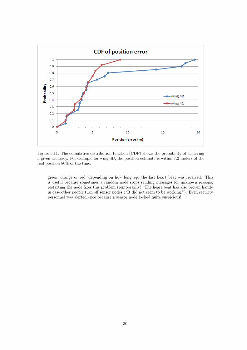
Figure 5.11: The cumulative distribution function (CDF) shows the probability of achievinga given accuracy. For example for wing 4B, the position estimate is within 7.2 meters of thereal position 80% of the time.

green, orange or red, depending on how long ago the last heart beat was received. Thisis useful because sometimes a random node stops sending messages for unknown reasons;restarting the node fixes this problem (temporarily). The heart beat has also proven handyin case other people turn off sensor nodes (“It did not seem to be working.”). Even securitypersonnel was alerted once because a sensor node looked quite suspicious!

30

Chapter 6

Conclusion

We have discussed the most relevant techniques for indoor localization in Wireless Sensor Networks,being lateration, angulation, and scene analysis. Furthermore, a comparison was made betweenseveral localization systems. We can conclude that the choice for a certain system or techniquedepends on the intended application. The application requirements therefore determine for a greatdeal which hardware and software setup is feasible.

A prototype of a system for determining the position of a moving device has been developed.With some help of the user, the system can adapt itself to its environment within limited time bylearning the relation between distance and signal strength. The primary goal, showing the relativepositions of deployed sensor nodes on a map which is to be displayed on a PDA, has been achieved.The system’s main advantage over most other existing systems is its short deployment time in anew environment while still achieving a reasonable accuracy. Furthermore, the developed system isnot limited to indoor environments. It can be adapted easily to other environments by performingautomatic function fitting on a radio propagation model suited for the specific environment (e.g.,outdoor).

The requirements of the application were validated. Improvements can be made with respectto accuracy and mobility. The accuracy requirements were met in a small open workspace envi-ronment. Multipath effects and obstructions such as walls and pillars were found to be causes ofposition errors. To be able to reach the desired accuracy in a large space, a relatively simple solu-tion would be to increase the number of anchor nodes. However, this would also increase the costof the system. Another way to improve accuracy would be to use a wall attenuation model, whichsystems such as RADAR and OPT employ. Such a model compensates for walls between senderand receiver. Our model could be extended with a wall model by adapting the fitting function.Measurements made during learning and localization should then be corrected for the number ofwalls between sender and receiver. Furthermore, adding wall information to maps should be madepossible in the user interface, or this information should be inferred from a map by the system tosave deployment time. This extension has not been built into the system due to time limitations.

To better support a moving user, the mobile node could be attached to an accelerometer todetect if it is moving. If it is, an approach similar to the Trajectory Matching (TM) system can beused to locate the mobile user. In case the node is stationary, our system is used for positioningbecause TM can only localize a moving sensor node.

31

Bibliography

[1] Xueli An, Jing Wang, R. Venkatesha Prasad, and I. G. M. M. Niemegeers. OPT: onlineperson tracking system for context-awareness in wireless personal network. In REALMAN’06: Proceedings of the 2nd International Workshop on Multi-hop Ad Hoc Networks: fromTheory to Reality, pages 47–54, New York, NY, USA, 2006. ACM.

[2] Atmel. AT86RF230 – Low power 2.4 GHz radio transceiver for ZigBee and IEEE 802.15.4 ap-plications. http://www.atmel.com/dyn/products/product card.asp?part id=3941, December2007.

[3] Paramvir Bahl and Venkata N. Padmanabhan. RADAR: An in-building RF-based user loca-tion and tracking system. pages 775–784, Tel-Aviv, Israel, March 2000. IEEE Infocom.

[4] Can Basaran. A hybrid localization algorithm for wireless sensor networks. Master’s thesis,Yeditepe University, Turkey, July 2007.

[5] T. Bokareva, W. Hu, S. Kanhere, B. Ristic, N. Gordon, T. Bessel, M. Rutten, and S. Jha.Wireless sensor networks for battlefield surveillance. Proceedings of Land Warfare Conference2006, October 2006.

[6] Srdjan Capkun, Maher Hamdi, and Jean-Pierre Hubaux. GPS-free positioning in mobile adhoc networks. Cluster Computing, 5(2):157–167, 2002.

[7] Youssef Chraibi. Localization in wireless sensor networks. Master’s thesis, Royal Institute ofTechnology, Sweden, November 2005.

[8] Crossbow. Application note, Avoiding RF interference between WiFi and ZigBee.http://www.xbow.com/Support/Support pdf files/ZigBeeandWiFiInterference.pdf.

[9] Crossbow. IRIS data sheet. http://www.xbow.com/Products/Product pdf files/Wireless pdf/IRIS Datasheet.pdf.

[10] Crossbow. MDA300 data acquisition board. http://www.xbow.com/Products/Product pdf files/Wireless pdf/MDA300CA Datasheet.pdf.

[11] David M. Doolin and Nicholas Sitar. Wireless sensors for wildfire monitoring. In MasayoshiTomizuka, editor, Smart Structures and Materials 2005: Sensors and Smart Structures Tech-nologies for Civil, Mechanical, and Aerospace Systems, volume 5765, pages 477–484. SPIE,2005.

[12] E. Elnahrawy, Xiaoyan Li, and R. P. Martin. The limits of localization using signal strength:a comparative study. In Proceedings of the First Annual IEEE Communications SocietyConference on Sensor and Ad Hoc Communications and Networks (SECON ’04), pages 406–414, October 2004.

[13] Rodrigo Fonseca, Omprakash Gnawali, Kyle Jamieson, Sukun Kim, Philip Levis, andAlec Woo. TinyOS Extension Proposal 123: The Collection Tree Protocol (CTP).http://www.tinyos.net/tinyos-2.x/doc/html/tep123.html, February 2007. Draft-Version 1.8.

32

[14] Rodrigo Fonseca, Omprakash Gnawali, Kyle Jamieson, and Philip Levis. TinyOS ExtensionProposal 119: Collection. http://www.tinyos.net/tinyos-2.x/doc/html/tep119.html, Febru-ary 2006.

[15] Rodrigo Fonseca, Omprakash Gnawali, Kyle Jamieson, and Philip Levis. Four-bit wirelesslink estimation. Technical Report SING-07-00, UC Berkeley, Univ. of Southern California,MIT CSAIL, Stanford Univ., 2007.

[16] Erik Haas. Design, Evaluation and Implementation of a Multi-Carrier Transmission Systemfor Aeronautical Communications. Herbert Utz Verlag, Munich, Germany, 2003.

[17] Carl Hartung, Richard Han, Carl Seielstad, and Saxon Holbrook. FireWxNet: a multi-tieredportable wireless system for monitoring weather conditions in wildland fire environments. InMobiSys ’06: Proceedings of the 4th international conference on Mobile systems, applicationsand services, pages 28–41, New York, NY, USA, 2006. ACM.

[18] Tian He, Sudha Krishnamurthy, Liqian Luo, Ting Yan, Lin Gu, Radu Stoleru, Gang Zhou,Qing Cao, Pascal Vicaire, John A. Stankovic, Tarek F. Abdelzaher, Jonathan Hui, and BruceKrogh. VigilNet: An integrated sensor network system for energy-efficient surveillance. ACMTransactions on Sensor Networks (TOSN), 2(1):1–38, 2006.

[19] Jeffrey Hightower and Gaetano Borriello. A survey and taxonomy of location systems forubiquitous computing. Technical Report UW-CSE 01-08-03, University of Washington, Com-puter Science and Engineering, Seattle, WA, USA, August 2001.

[20] Ville A. Kaseva, Mikko Kohvakka, Mauri Kuorilehto, Marko Hnnikinen, and Timo D. Hmli-nen. A wireless sensor network for RF-based indoor localization. In EURASIP Journal onAdvances in Signal Processing, volume 2008, 2008.

[21] Stuart Kininmonth, Scott Bainbridge, Ian Atkinson, Eric Gill, Laure Barral, and RomainVidaud. Sensor networking the Great Barrier Reef. Spatial Sciences Queensland Journal,pages 34–38, Spring 2004.

[22] Koen Langendoen and Niels Reijers. Distributed localization in wireless sensor networks: aquantitative comparison. Computer Networks, 43(4):499–518, 2003.

[23] HyungJune Lee, Martin Wicke, Branislav Kusy, and Leonidas Guibas. Localization of mobileusers using trajectory matching. In MELT ’08: Proceedings of the first ACM InternationalWorkshop on Mobile Entity Localization and Tracking in GPS-less Environments, pages 123–128, New York, NY, USA, 2008. ACM.

[24] Yanjun Li, Zhi Wang, and Yeqiong Song. Wireless sensor networks for wildfire monitoring.The Sixth World Congress on Intelligent Control and Automation (WCICA 2006), June 2006.

[25] M.E.M. Lijding, H.P. Benz, N. Meratnia, and P.J.M. Havinga. Smart Signs: Showing theway in smart surroundings. Technical Report TR-CTIT-06-20, Centre for Telematics andInformation Technology, University of Twente, Enschede, 2006.

[26] Konrad Lorincz and Matt Welsh. Motetrack: a robust, decentralized approach to RF-basedlocation tracking. Personal Ubiquitous Computing, 11(6):489–503, 2007.

[27] Alan Mainwaring, David Culler, Joseph Polastre, Robert Szewczyk, and John Anderson.Wireless sensor networks for habitat monitoring. In WSNA ’02: Proceedings of the 1st ACMInternational Workshop on Wireless Sensor Networks and Applications, pages 88–97, NewYork, NY, USA, 2002. ACM.

[28] Guoqiang Mao, Barıs Fidan, and Brian D.O. Anderson. Wireless sensor network localizationtechniques. Computer Networks, 51(10):2529–2553, July 2007.

33

[29] Miklos Maroti, Branislav Kusy, Gyula Simon, and Akos Ledeczi. The flooding time syn-chronization protocol. In SenSys ’04: Proceedings of the 2nd International Conference onEmbedded Networked Sensor Systems, pages 39–49, New York, NY, USA, 2004. ACM.

[30] MIT Computer Science and Artificial Intelligence Lab, Cambridge, MA, USA. Cricket v2User Manual, January 2005. http://cricket.csail.mit.edu/.

[31] David Moore, John Leonard, Daniela Rus, and Seth Teller. Robust distributed network local-ization with noisy range measurements. In SenSys ’04: Proceedings of the 2nd InternationalConference on Embedded Networked Sensor Systems, pages 50–61, New York, NY, USA, 2004.ACM.

[32] Nissanka B. Priyantha, Hari Balakrishnan, Erik D. Demaine, and Seth Teller. Mobile-assistedlocalization in wireless sensor networks. Proceedings of IEEE INFOCOM ’05, 1:172–183,March 2005.

[33] Nissanka B. Priyantha, Anit Chakraborty, and Hari Balakrishnan. The Cricket location-support system. In MobiCom ’00: Proceedings of the 6th Annual International Conferenceon Mobile Computing and Networking, pages 32–43, New York, NY, USA, 2000. ACM.

[34] Sven Rienstra and Serhat Gulcicek. Wireless sensor networks. Bachelor’s thesis, SaxionHogeschool Enschede, Netherlands, June 2008.

[35] Andreas Savvides, Mani Srivastava, Lewis Girod, and Deborah Estrin. Localization in sen-sor networks. In Wireless Sensor Networks, chapter 15, pages 327–349. Kluwer AcademicPublishers, Norwell, MA, USA, 2004.

[36] Spread Spectrum Scene. An introduction to indoor radio propagation. http://sss-mag.com/indoor.html, June 2001.

[37] Adam Smith, Hari Balakrishnan, Michel Goraczko, and Nissanka Bodhi Priyantha. TrackingMoving Devices with the Cricket Location System. In 2nd International Conference on MobileSystems, Applications and Services (Mobisys 2004), Boston, MA, USA, June 2004.

[38] William Stallings. Data and Computer Communications. Prentice Hall, 8th edition, 2007.

[39] Tsenka Stoyanova, Fotis Kerasiotis, Aggeliki Prayati, and George Papadopoulos. Evaluationof impact factors on RSS accuracy for localization and tracking applications. In MobiWac ’07:Proceedings of the 5th ACM International Workshop on Mobility Management and WirelessAccess, pages 9–16, New York, NY, USA, 2007. ACM.

[40] M. Terwilliger, A. Gupta, V. Bhuse, Z. Kamal, and M. Salahuddin. A localization systemusing wireless network sensors: a comparison of two techniques. In Proceedings of the 1stWorkshop on Positioning, Navigation and Communication (WPNC ’04), Hanover, Germany,March 2004.

[41] Mark Terwilliger. Localization in wireless sensor networks. PhD thesis, Western MichiganUniversity, Kalamazoo, MI, USA, April 2006.

[42] Brett Warneke, Matt Last, Brian Liebowitz, and Kristofer S. J. Pister. Smart Dust: Com-municating with a cubic-millimeter computer. Computer, 34(1):44–51, 2001.

[43] Adel Amin Abdel Azim Youssef. SALAM: a scalable anchor-free localization algorithm forwireless sensor networks. PhD thesis, University of Maryland, College Park, MD, USA, 2006.

[44] Pei Zheng and Lionel Ni. Smart Phone and Next Generation Mobile Computing. MorganKaufmann, 2005.

34