Embed Size (px)
Citation preview
SCALABLE SENSOR LOCALIZATION ALGORITHMS
FOR WIRELESS SENSOR NETWORKS
by
Holly Hui Jin
A thesis submitted in conformity with the requirementsfor the degree of Doctor of Philosophy
Graduate Department of Mechanical and Industrial EngineeringUniversity of Toronto
Copyright c© 2005 by Holly Hui Jin
Abstract
SCALABLE SENSOR LOCALIZATION ALGORITHMS
FOR WIRELESS SENSOR NETWORKS
Holly Hui Jin
Doctor of Philosophy
Graduate Department of Mechanical and Industrial Engineering
University of Toronto
2005
An adaptive rule-based algorithm, SpaseLoc, is described to solve localization problems
for ad hoc wireless sensor networks. A large problem is solved as a sequence of very
small subproblems, each of which is solved by semidefinite programming relaxation of
a geometric optimization model. The subproblems are generated according to a set of
sensor/anchor selection rules and a priority list. Computational results compared with
existing approaches show that the SpaseLoc algorithm scales well and provides excellent
positioning accuracy.
A dynamic version of the SpaseLoc method is developed for estimating moving sensors
locations in a real-time environment. The method uses dynamic distance measurement
updates among sensors, and utilizes SpaseLoc for static sensor localization. Further
computational results are presented, along with an application to bus transit systems.
Ways to deploy sensor localization algorithms in clustered distributed environments
are also studied, permitting application to arbitrarily large networks. In addition, we
extend the algorithm to solving sensor localizations in 3D space. A preprocessor is
developed to enable SpaseLoc for localization of networks without absolute position in-
formation.
Joint research conducted in the Dept of Management Science and Engineering, Stanford University.
ii

To my parents
iii
Acknowledgements
I would like to express my greatest appreciation towards my two thesis advisors, Prof. Michael
Carter and Prof. Michael Saunders, for their continuous guidance, support and friendship.
My sincere gratitude goes to Prof. Carter for accepting me into the PhD program and for
keeping constant faith in me. No matter what new project I start up, he is always supportive
and remarkably perceptive in advising in the right direction and correcting the vital details.
Without his continuous encouragement, I would still be in my PhD dreams. He is a great
mentor and I learned so much from him through this long academic journey.
I am truly blessed to have come to Stanford University, where Prof. Saunders welcomed me
with open arms and my life started on a whole new course. I learn from Prof. Saunders that
the world is not just about optimization, but more about true kindness. He is the epitome
of professionalism and perfectionism. I could not have finished my thesis in time without his
untiring help in making every sentence concise and correct. I will always be looking up to the
high standard he sets.
I would like to thank Prof. Yinyu Ye for inspiring me to the exciting field of sensor network
research. I am very fortunate to be able to learn from him and his class. His work with Pratik
Biswas was a vital starting point for my thesis. I am grateful to Dr. Steve Benson for his advice
on using the DSDP5.0 solver. I also appreciate Prof. Kenneth Holmstrom’s help in fine-tuning
the Matlab implementation of some portions of SpaseLoc.
My thesis committee members, Profs. Daniel Francis, Scott Rogers, and Henry Wolkowicz,
provided invaluable feedback and advice on my thesis. I really appreciate their time and help.
Thanks to the University of Toronto for making my PhD studies there possible with the
prestigious Connaught scholarships. Its outstanding learning environment helped lay a solid
academic foundation. I must also thank Stanford University for two years of my PhD studies
there. Its invigorating environment enabled my mind to broaden and my research to thrive.
I am grateful to Robert Bosch Corporation’s support of my research at Stanford University.
I feel very fortunate for the opportunity to discuss potential applications of our sensor localiza-
tion algorithms with the talented Bosch team, Sharmila Ravula, Bhaskar Srinivasan, Lakshmi
Venkatraman, Hauke Schmidt, and Karsten Funk. They provided inspiration and background
for our algorithms to be practically useful.
I am indebted to my husband Neil for his encouragement and understanding when I devoted
too many evenings and weekends to my thesis study, and he had to look after our two beautiful
children Danlin and Hansen while carrying a full time workload himself. Thank you so much
Neil for all the mornings when you took the kids quietly out of the house in the weekends so
that I could sleep in a bit after late night studying at school. Thank you Danlin and Hansen
for many nights not be able to kiss you goodnight and you still give me so much love and joy.
Finally, I give heartfelt thanks to my dearest parents, my sister and my two brothers for
their unyielding love and support. They provide a constant source of motivation in my life.
iv
Contents
1 Introduction 1
1.1 Problem Definition . . . . . . . . . . . . . . . . . . . . . . . . . . . . . . 2
1.2 Notation . . . . . . . . . . . . . . . . . . . . . . . . . . . . . . . . . . . . 3
1.3 Related Research Work . . . . . . . . . . . . . . . . . . . . . . . . . . . . 4
1.4 Solution Techniques . . . . . . . . . . . . . . . . . . . . . . . . . . . . . . 5
1.5 Thesis Outline . . . . . . . . . . . . . . . . . . . . . . . . . . . . . . . . . 6
2 The Subproblem SDP Model 7
2.1 Euclidean Distance Model . . . . . . . . . . . . . . . . . . . . . . . . . . 7
2.2 The Euclidean Distance Model in Matrix Form . . . . . . . . . . . . . . . 9
2.3 The SDP Relaxation Model . . . . . . . . . . . . . . . . . . . . . . . . . 10
2.4 SDP Model Analysis . . . . . . . . . . . . . . . . . . . . . . . . . . . . . 11
3 SpaseLoc: A Scalable Localization Algorithm 12
3.1 Adaptive Subproblem Approach . . . . . . . . . . . . . . . . . . . . . . . 12
3.1.1 The SpaseLoc Algorithm . . . . . . . . . . . . . . . . . . . . . . . 13
3.1.2 Subproblem Creation Procedure . . . . . . . . . . . . . . . . . . . 15
3.1.3 Subsensor Selection Priority List . . . . . . . . . . . . . . . . . . 17
3.1.4 Subanchors Selection . . . . . . . . . . . . . . . . . . . . . . . . . 19
3.1.5 Independent Subanchors Selection . . . . . . . . . . . . . . . . . . 19
3.1.6 Geometric Subroutine (Two Connected Anchors) . . . . . . . . . 20
3.1.7 Geometric Subroutine (One Connected Anchor) . . . . . . . . . . 22
3.2 An Example . . . . . . . . . . . . . . . . . . . . . . . . . . . . . . . . . . 24
3.3 Computational Results . . . . . . . . . . . . . . . . . . . . . . . . . . . . 27
3.3.1 Effect of Inequality Constraints in SDP Relaxation Model . . . . 28
3.3.2 Accuracy and Speed Comparison: Full SDP vs SpaseLoc . . . . . 32
3.3.3 Scalability . . . . . . . . . . . . . . . . . . . . . . . . . . . . . . . 35
3.3.4 Radio Range Impact . . . . . . . . . . . . . . . . . . . . . . . . . 36
v
3.3.5 Noise Factor Impact . . . . . . . . . . . . . . . . . . . . . . . . . 37
3.3.6 Number of Anchors Impact . . . . . . . . . . . . . . . . . . . . . 37
3.3.7 Number of Anchors Impact with Noise . . . . . . . . . . . . . . . 38
3.3.8 Anchors Impact with Noise and Lower radius . . . . . . . . . . . 39
4 Moving Sensor Localizations 40
4.1 Moving Sensor Localization Method . . . . . . . . . . . . . . . . . . . . . 40
4.1.1 Problem Formulation . . . . . . . . . . . . . . . . . . . . . . . . . 41
4.1.2 Moving Sensor Identification Routine . . . . . . . . . . . . . . . . 42
4.1.3 Moving Sensor Localization Procedure . . . . . . . . . . . . . . . 44
4.2 Moving Sensor Simulation Results . . . . . . . . . . . . . . . . . . . . . . 46
4.2.1 Moving Sensor Performance: 10% Moving Sensors . . . . . . . . . 47
4.2.2 Effect of Number of Moving Sensors . . . . . . . . . . . . . . . . . 48
4.2.3 Sensor Speed versus Number of Sensors Algorithm Can Track . . 49
4.3 Applications of the Moving Sensor Localization Algorithm . . . . . . . . 51
4.3.1 Battlefield Tracking System . . . . . . . . . . . . . . . . . . . . . 51
4.3.2 Police Patrol Car Monitoring and Dispatching System . . . . . . . 52
4.3.3 Car Tracking in a Car-share Network . . . . . . . . . . . . . . . . 52
4.3.4 Traffic Monitoring System . . . . . . . . . . . . . . . . . . . . . . 53
4.3.5 Personnel Monitoring System . . . . . . . . . . . . . . . . . . . . 53
4.3.6 Bus Transit Arrival Reporting System . . . . . . . . . . . . . . . 54
5 Distributed Algorithm For Clustered Networks 56
5.1 The Need for Distributed Computing . . . . . . . . . . . . . . . . . . . . 57
5.2 Clustered Sensor Network Architecture . . . . . . . . . . . . . . . . . . . 57
5.3 Distributed Sensor Localization Approach . . . . . . . . . . . . . . . . . 58
5.3.1 Sequencing of Parallel Processes . . . . . . . . . . . . . . . . . . . 59
5.3.2 Cluster Priority . . . . . . . . . . . . . . . . . . . . . . . . . . . . 61
5.3.3 Synchronization among Parallel Processes . . . . . . . . . . . . . 63
5.3.4 Distributed Sensor Localization Algorithm . . . . . . . . . . . . . 65
5.4 Distributed Algorithm Simulation Results . . . . . . . . . . . . . . . . . 66
5.4.1 Number of 3-anchor Clusters Impact . . . . . . . . . . . . . . . . 67
5.4.2 Number of 3-anchor Clusters Impact with Noise . . . . . . . . . . 70
5.4.3 Node Density Impact . . . . . . . . . . . . . . . . . . . . . . . . . 70
5.4.4 Radio Range Impact . . . . . . . . . . . . . . . . . . . . . . . . . 71
5.4.5 Noise Factor Impact . . . . . . . . . . . . . . . . . . . . . . . . . 72
vi
5.4.6 Number of Clusters Impact . . . . . . . . . . . . . . . . . . . . . 72
6 3D Extensions 74
6.1 3D Sensor Localization Geometry . . . . . . . . . . . . . . . . . . . . . . 74
6.2 3D Localization Design . . . . . . . . . . . . . . . . . . . . . . . . . . . . 75
6.3 3D Localization Simulation Results . . . . . . . . . . . . . . . . . . . . . 76
6.3.1 Scalability . . . . . . . . . . . . . . . . . . . . . . . . . . . . . . . 77
6.3.2 Radio Range Impact . . . . . . . . . . . . . . . . . . . . . . . . . 78
6.3.3 Noise Factor Impact . . . . . . . . . . . . . . . . . . . . . . . . . 78
6.3.4 Number of Anchors Impact . . . . . . . . . . . . . . . . . . . . . 79
6.3.5 Number of Anchors Impact with Noise . . . . . . . . . . . . . . . 79
6.3.6 Number of Anchors Impact with Noise and Lower radius . . . . . 80
7 Sensor Localization in Anchorless Networks 81
7.1 Anchorless Networks . . . . . . . . . . . . . . . . . . . . . . . . . . . . . 81
7.2 Surrogate Anchor Selection . . . . . . . . . . . . . . . . . . . . . . . . . . 82
7.3 An Example . . . . . . . . . . . . . . . . . . . . . . . . . . . . . . . . . . 84
8 Conclusions and Future Research 86
8.1 Contributions . . . . . . . . . . . . . . . . . . . . . . . . . . . . . . . . . 86
8.2 Impact of the Research . . . . . . . . . . . . . . . . . . . . . . . . . . . . 88
8.3 Future Research . . . . . . . . . . . . . . . . . . . . . . . . . . . . . . . . 89
Molecular structure identification . . . . . . . . . . . . . . . . . . 89
Cartography . . . . . . . . . . . . . . . . . . . . . . . . . . . . . . 89
General version of distributed algorithm . . . . . . . . . . . . . . 89
Objective function with `2 norm . . . . . . . . . . . . . . . . . . . 89
Porting codes to C . . . . . . . . . . . . . . . . . . . . . . . . . . 90
Conversions between absolute locations and digital map . . . . . . 90
Deployment to real-world applications . . . . . . . . . . . . . . . 91
Bibliography 92
vii
List of Tables
3.1 An example: priority list when MaxAnchorReq=3. . . . . . . . . . . . . . 18
3.2 Inequality impact on accuracy and speed: 100 nodes, 10 anchors, no noise,
radius 0.2275. . . . . . . . . . . . . . . . . . . . . . . . . . . . . . . . . . 30
3.3 Inequality impact on accuracy and speed: 100 nodes, 10 anchors, noise factor
0.1, radius 0.25. . . . . . . . . . . . . . . . . . . . . . . . . . . . . . . . . 31
3.4 Accuracy and speed comparison between full SDP and SpaseLoc. . . . . 33
3.5 SpaseLoc scalability. Strategies I2, I1, and I0 generate same results. . . . 35
3.6 Radio range impact: nodes = 3969, anchors = 63, no noise. . . . . . . . . 37
3.7 Noise factor impact: nodes = 3969, anchors = 63, radius = 0.033, sub-
problem size = 3. . . . . . . . . . . . . . . . . . . . . . . . . . . . . . . . 37
3.8 Number of anchors impact: nodes = 3969, radius = 0.033, no noise, sub-
problem size = 3. . . . . . . . . . . . . . . . . . . . . . . . . . . . . . . . 38
3.9 Number of anchors impact: nodes = 3969, radius = 0.033, noise factor =
0.1, subprob size = 3. . . . . . . . . . . . . . . . . . . . . . . . . . . . . . 38
3.10 Number of anchors impact: nodes = 3969, radius = 0.026, noise factor =
0.1, subprob size = 5. . . . . . . . . . . . . . . . . . . . . . . . . . . . . . 39
4.1 Moving sensor performance: 10% moving sensors . . . . . . . . . . . . . 47
4.2 Effect of number of moving sensors: Anchors = 63, radius = 0.033, sub-
problem size = 9, no noise . . . . . . . . . . . . . . . . . . . . . . . . . . 48
4.3 Number of moving sensors that can be tracked versus speed of movement:
Anchors = 63, radius = 0.033, subproblem size = 9, no noise, speed in
miles/hr, time in milliseconds . . . . . . . . . . . . . . . . . . . . . . . . 50
5.1 Cluster priority: an example . . . . . . . . . . . . . . . . . . . . . . . . . 64
5.2 Cluster priorities for example in Figure 5.1 . . . . . . . . . . . . . . . . . 64
5.3 Cluster rank list for example in Figure 5.1 . . . . . . . . . . . . . . . . . 66
5.4 Number of 3-anchor clusters impact: 25 clusters, 4900 total nodes, 196
nodes in each cluster, radius 0.1, no noise . . . . . . . . . . . . . . . . . . 69
viii
5.5 Number of 3-anchor clusters impact with noise: 25 clusters, 4900 total
nodes, 196 nodes in each cluster, radius 0.1, with noise factor = 0 .1 . . . 70
5.6 Node density impact with number of clusters = 25, number of 3-anchor
clusters = 8, radius = 0.100; noise factor = 0 . . . . . . . . . . . . . . . 71
5.7 Radio range impact with nodes = 4900, number of clusters = 25, number
of 3-anchor clusters = 8, noise factor = 0 . . . . . . . . . . . . . . . . . 71
5.8 Noise factor impact with nodes = 4900, number of clusters = 25, number
of 3-anchor clusters = 8, radius = 0.1 . . . . . . . . . . . . . . . . . . . . 72
5.9 Number of clusters impact with 256 nodes in each cluster; all 3-anchor
clusters . . . . . . . . . . . . . . . . . . . . . . . . . . . . . . . . . . . . . 73
6.1 3D algorithm scalability. . . . . . . . . . . . . . . . . . . . . . . . . . . . 77
6.2 Radio-range impact: nodes = 4096, anchors = 256, no noise. . . . . . . . 78
6.3 Noise factor impact: nodes = 4096, anchors = 256, radius = 0.15. . . . . 78
6.4 Number of anchors impact: nodes = 4096, radius = 0.15, no noise. . . . . 79
6.5 Number of anchors impact: nodes = 4096, radius = 0.150, noise factor =
0.1. . . . . . . . . . . . . . . . . . . . . . . . . . . . . . . . . . . . . . . . 79
6.6 Number of anchors impact: nodes = 4096, radius = 0.125, noise factor =
0.1 . . . . . . . . . . . . . . . . . . . . . . . . . . . . . . . . . . . . . . . 80
ix
List of Figures
1.1 Indexing of sensors and anchors. . . . . . . . . . . . . . . . . . . . . . . . 3
3.1 SpaseLoc execution time as a function of subproblem size: total nodes =
10000, anchors = 100, radius = 0.02068. . . . . . . . . . . . . . . . . . . 14
3.2 Sensors with connections to at most two anchors. . . . . . . . . . . . . . 20
3.3 (a) Sensor with two anchors’ circles intersecting. (b) Sensor with two
anchors, a2’s circle in a3’s. (c) Sensor with two anchors’ circles disjoint. . 21
3.4 (a) Sensor with one anchor connection a and one neighboring anchor b.
(b) Sensor with one anchor connection a and two neighboring anchors b, c. 23
3.5 An example. . . . . . . . . . . . . . . . . . . . . . . . . . . . . . . . . . . 24
3.6 Inequality impact on accuracy: 100 nodes, 10 anchors, no noise, radius
0.2275. . . . . . . . . . . . . . . . . . . . . . . . . . . . . . . . . . . . . . 30
3.7 Inequality impact on accuracy: 100 nodes, 10 anchors, noise factor 0.1,
radius 0.25. . . . . . . . . . . . . . . . . . . . . . . . . . . . . . . . . . . 31
3.8 9 nodes on equilateral-triangle grids, 3 anchors, 0.1 noise, radius 1.12. . . 34
3.9 49 nodes on equilateral-triangle grids, 7 anchors, 0.1 noise, radius 0.40. . 34
3.10 SDP computational complexity . . . . . . . . . . . . . . . . . . . . . . . 36
4.1 An example of moving sensors. . . . . . . . . . . . . . . . . . . . . . . . . 45
4.2 Sensors moving at same speed. . . . . . . . . . . . . . . . . . . . . . . . . 45
4.3 One moving sensor, 400 total points, 20 anchors, radius 0.1078, no noise . 47
4.4 Bus transit simulation, 400 total points, 38 anchors, radius 0.0819, no noise 55
5.1 An example of a sensor network with 25 clusters. . . . . . . . . . . . . . 60
5.2 An example of distributed localization, with 625 total points, 25 clusters,
25 nodes in each cluster, radius 0.16, no noise . . . . . . . . . . . . . . . 67
5.3 Topologies of different numbers of 3-anchor clusters. . . . . . . . . . . . . 68
6.1 Localization errors for 3D localization with geometric routine. . . . . . . 76
x
6.2 3D sensor localization, 100 total points, 15 anchors, radius 0.5, no noise . 77
7.1 Example anchorless network. The entry σ is√
2. . . . . . . . . . . . . . . 84
7.2 An example of anchorless localization, radius√
2, no noise . . . . . . . . 85
8.1 Accuracy and performance comparison. . . . . . . . . . . . . . . . . . . . 87
8.2 Hierarchical algorithm structure. . . . . . . . . . . . . . . . . . . . . . . 88
xi
Chapter 1
Introduction
Ad hoc wireless sensor networks may contain hundreds or even tens of thousands of in-
expensive devices (sensors) that can communicate with their neighbors within a limited
radio range. By relaying information to each other, they can transmit signals to a com-
mand post anywhere within the network. They have many practical uses in areas such
as military applications [27], environment or industrial control and monitoring [11, 13],
wildlife monitoring [45], and security monitoring [27]. For example, Southern Califor-
nia Edison’s Nuclear Generating Station in San Onofre, California has deployed wireless
mesh networked sensors from Dust Networks to obtain real-time trend data [13]. These
data are used to predict which motors are about to fail, so they could be preemptively
rebuilt or replaced during scheduled maintenance periods. The use of a wireless sensor
network saves the station money and avoids potential machine shutdown. Implementa-
tion of a sensor localization algorithm would provide a service that eliminates the need
to record every sensor’s location and its associated ID number in the network.
Wireless sensor networks are potentially important enablers for many other advanced
applications. A huge variety of applications lie ahead. By 2008, there could be 100 million
wireless sensors in use, up from about 200,000 in 2005, according to the market-research
company Harbor Research. The worldwide market for wireless sensors, it says, will grow
from $100 million in 2005 to more than $1 billion by 2009 [36]. This is motivating great
effort in academia and industry to explore effective ways to build sensor networks with
feature-rich services [19].
One of the important inputs these services build upon is the exact locations of all
sensors in the network. The need for sensor localization arises because accurate positions
are known for only some of the sensors (which are called anchors). If the networks are
to achieve their purpose, the positions of the remaining sensors must be determined.
One approach to localizing these sensors with unknown positions is to use known anchor
1
Chapter 1. Introduction 2
locations and distance measurements that neighboring sensors and anchors obtain among
themselves. The mathematical problem is to estimate sensor positions using a sparse data
matrix of noisy distance measurements. This leads to a large, non-convex, constrained
optimization problem. Large networks may contain many thousands of sensors, whose
locations should be determined accurately and quickly.
One way to localize a sensor is to rely on the satellite-based global positioning system
(GPS) [9]. This may be important for at least some of the sensors in a network. (They
would be anchors.) However, GPS suffers the following main drawbacks:
• GPS based system is typically more expensive to deploy because devices using it
are more costly.
• GPS can be less accurate. Without the use of specialized equipment, normal GPS
can pin point subject locations with 5 to 10 meter accuracy in outdoor environment.
• GPS is not applicable for indoor localization since GPS requires line of sight.
• Because of satellite communication delay, use of GPS might not be an effective
method for real-time tracking of moving sensors.
Existing non-GPS-based localization methods have been applicable for only moderate-
sized networks. The primary aim of this thesis is to develop non-GPS-based localization
algorithms that are effective for the large-scale networks that are likely to be deployed
in the coming decades, and to achieve the efficiency needed for real-time environments.
In this chapter we first describe the sensor localization problem and introduce relevant
notation. A review of related research work follows. Our new solution techniques are
summarized next, and finally the thesis outline is given.
1.1 Problem Definition
Sensor localization in ad hoc wireless sensor network aims to find the locations of all
sensors in the network, given pair-wise distance measurements among some of the sensors,
and known locations of some of the sensors. The sensors with known locations are called
anchors. From now on, sensor generally means unpositioned sensor, excluding anchors.
A node is any sensor or anchor in the network.
We use a constrained optimization approach to estimate the sensors’ locations. The
following input, output, and objectives are considered.
Chapter 1. Introduction 3
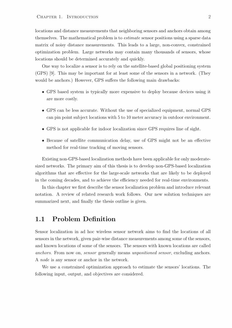
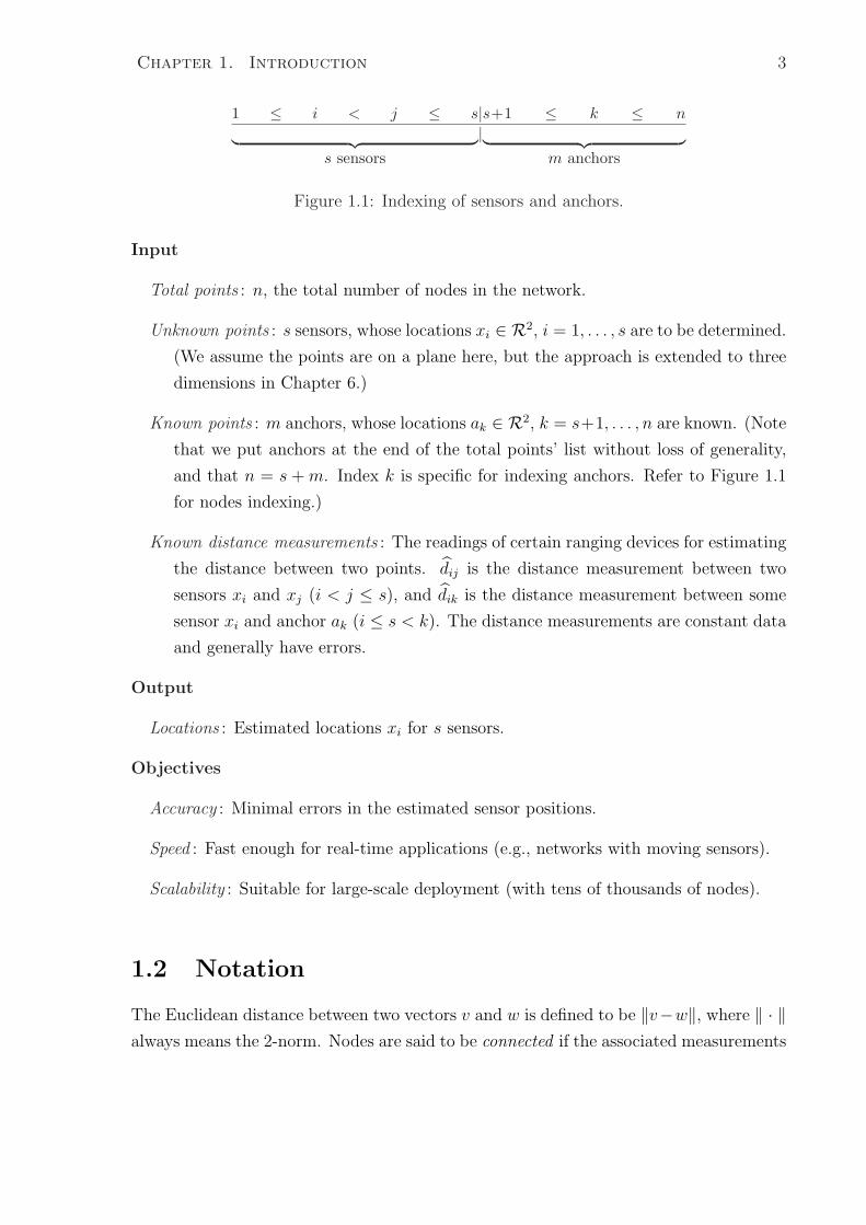
1 ≤ i < j ≤ s|s+1 ≤ k ≤ n
︸ ︷︷ ︸|︸ ︷︷ ︸s sensors m anchors
Figure 1.1: Indexing of sensors and anchors.
Input
Total points : n, the total number of nodes in the network.
Unknown points : s sensors, whose locations xi ∈ R2, i = 1, . . . , s are to be determined.
(We assume the points are on a plane here, but the approach is extended to three
dimensions in Chapter 6.)
Known points : m anchors, whose locations ak ∈ R2, k = s+1, . . . , n are known. (Note
that we put anchors at the end of the total points’ list without loss of generality,
and that n = s + m. Index k is specific for indexing anchors. Refer to Figure 1.1
for nodes indexing.)
Known distance measurements : The readings of certain ranging devices for estimating
the distance between two points. dij is the distance measurement between two
sensors xi and xj (i < j ≤ s), and dik is the distance measurement between some
sensor xi and anchor ak (i ≤ s < k). The distance measurements are constant data
and generally have errors.
Output
Locations : Estimated locations xi for s sensors.
Objectives
Accuracy : Minimal errors in the estimated sensor positions.
Speed : Fast enough for real-time applications (e.g., networks with moving sensors).
Scalability : Suitable for large-scale deployment (with tens of thousands of nodes).
1.2 Notation
The Euclidean distance between two vectors v and w is defined to be ‖v−w‖, where ‖ · ‖always means the 2-norm. Nodes are said to be connected if the associated measurements
Chapter 1. Introduction 4
dij or dik exist. The remaining elements of d are zero. If a measurement does exist between
node i and j but it is zero (i and j are at the same spot), we do not set dij to zero: we
set it to machine precision ε instead to distinguish from the case of dij = 0 when two
nodes’ distance is beyond the sensor device’s measuring range.
1.3 Related Research Work
Sensor localization in ad hoc wireless network has been a booming research area recently.
Hightower and Boriello [19] give an extensive review of the area and available methods.
There are many ways to solve the localization problem [2, 7, 12, 15, 20, 33, 37, 38, 39, 40],
with two main ones based on triangulation and optimization.
Triangulation methods estimate node positions based on distance measurements be-
tween neighboring nodes, and some algorithms use iterative steps to localize all sensors.
Early work using optimization techniques is reported by Doherty et al. [12]. Ideally
the Euclidean distance between neighboring nodes should be fitted in some near-equality
sense to the distance measurements:
‖xi − xj‖ ≈ dij and ‖xi − ak‖ ≈ dik. (1.1)
Doherty et al. formulate a convex optimization model by treating the constraints as
‖xi − xj‖ ≤ dij and ‖xi − ak‖ ≤ dik, and by including certain other convex constraints.
This formulation takes advantage of available optimization algorithms, including those
for convex optimization. However, the method needs sufficient anchors to be positioned
on the boundary of the localization area for it to work effectively.
Biswas and Ye [4] work with the near-equality constraints (1.1), and most importantly
they introduced a semidefinite programming (SDP) relaxation method in order to retain
the benefits of convex optimization. They report that their method yields more accuracy
under all conditions than the approach in [12].
The SDP relaxation approach can solve small problems effectively. The paper reports
a few seconds of laptop execution time for a 50-node localization problem. However, the
number of constraints in the SDP model is O(n2), where n is the number of nodes in the
network. Even a few hundred-node problem leads to excessive memory and computation
time by available SDP solvers such as DSDP (Benson, Ye, and Zhang [3]) and SeDuMi
(Sturm [44]). These solvers are effective for SDP problems with dimension and number
of constraints up to a few thousand.
Tseng [46] has presented a second-order cone programming (SOCP) relaxation model
Chapter 1. Introduction 5
that permits solution for problem sizes up to a few thousand using available SOCP
solvers. However, the additional relaxation of the original model usually generates larger
error rates, and the run-times are high. The author reports CPU times of 330 seconds
for 1000 nodes and 3 hours for 2000 nodes using SeDuMi 1.05 [44] and Matlab 6.1 on
a Linux PC.
Biswas and Ye [5] propose a decomposition scheme to overcome the scalability issue
with SDP solvers. The anchors in the network are first partitioned into many clusters
according to their physical positions, and sensors are assigned to these clusters if they
have a direct connection to one of the anchors. Each cluster formulates a subproblem,
and the subproblems are solved independently on each cluster using the SDP relaxation
of [4]. The paper reports results for randomly generated sensor networks of 4000 sensors
partitioned into 100 clusters strictly according to their geographic locations. Sensors with
distance connections to more than one cluster are included in multiple clusters. The final
estimation of their locations is determined by the cluster that gives the least estimated
errors. An execution time of about 4 minutes on a 1.2GHz Pentium laptop is reported
for this sized problem. The time could be reduced by using multiple CPUs.
Although Biswas and Ye [5] make large-scale sensor network localization possible by
decomposing the large-scale problem geographically, there are shortfalls in this approach
that may prevent its large-scale deployment. First of all, for any real deployment of a
wireless sensor network, localization algorithms should run in real-time, where minutes
could be too long and multiple CPUs could be too expensive. Secondly, since the partition
is strictly based on geographic locations, sensors near the border lines of a cluster may not
be positioned as accurately as they would be using other approaches. This is due to the
fact that each cluster may include only partial connection information for the bordering
sensors if the bordering sensors have connections with multiple clusters. Furthermore,
the SDP relaxation approach that their decomposition method is based on provides poor
accuracy on certain topologies with low anchor density or small radio range for even
medium-size networks (refer to section 3.3.2).
1.4 Solution Techniques
A basic tool that we have developed during this research is a rule-based iterative algo-
rithm named SpaseLoc (sub-problem algorithm for sensor localization). It is effective for
networks involving tens of thousands of sensors and beyond.
To solve a large localization problem (defined as the full problem), SpaseLoc proceeds
iteratively by estimating only a portion of the total sensors’ locations at each iteration.
Chapter 1. Introduction 6
Some anchors and sensors are chosen according to a set of rules. They form a sensor
localization subproblem that can be treated similarly to the basic SDP formulation of
Biswas and Ye [4]. The solution from the subproblem is fed back to the full problem and
the algorithm iterates again until all sensors are localized.
Computational results show that SpaseLoc can solve small or large problems with
excellent accuracy and scalability. It is capable of localizing 4000 nodes with great
accuracy in under 20 seconds, and 10000 nodes in about a minute on a 2.4GHz laptop.
With the SpaseLoc tool in hand, we are able to develop a dynamic sensor localization
algorithm to track hundreds or thousands of sensors moving within a larger network. We
also develop distributed methods for deploying SpaseLoc in arbitrarily large networks. A
3D version of SpaseLoc extends its utility further. In addition, a preprocessor is designed
to allow SpaseLoc to be applied to sensor localizations in anchorless networks.
1.5 Thesis Outline
The basic sensor localization concept and current methods are described in the first
chapter. Chapter 2 introduces the semidefinite programming model that our SpaseLoc
subproblem is based on. We present our sensor localization algorithm SpaseLoc and
computational results in Chapter 3.
In Chapter 4, a dynamic version of SpaseLoc is developed for estimating moving
sensors’ locations in a real-time environment. The method uses dynamic distance mea-
surement updates among sensors, and utilizes SpaseLoc for static sensor localization.
Computational results for the algorithm are presented, along with an application to bus
transit systems.
Chapter 5 describes ways to deploy sensor localization algorithms in clustered dis-
tributed environments for true scalability.
In Chapter 6, we extend the algorithm to solving sensor localizations in 3D space.
In order for SpaseLoc to apply to networks containing no anchors, a preprocessor is
developed in Chapter 7 to obtain relative positions of all sensors in the network.
The last chapter summarizes, and points out future promising research areas.
Chapter 2
The Subproblem SDP Model
This chapter reviews the quadratic programming formulation of the sensor localization
problem, and the SDP relaxation model of Biswas and Ye [4] on which the SpaseLoc
subproblem is based. Error analysis is also reviewed here as a reference for later chapters.
2.1 Euclidean Distance Model
Consider a network of sensors and anchors labeled as in Figure 1.1. For any point in
the network, there could be three types of distance measurements. Since we generally
do not need the distance information between two anchor points, we exclude this type of
measurement from now on.
The other types of distance measurements are the two we need for the localization
model. First is the distance measurement between two sensors (i and j) with unknown
positions; second is the distance measurement between a sensor (i) and an anchor (k)
with known position. Corresponding to these two types of distances, we define sets N1,
N1, N2 and N2 as follows:
• N1 includes pairwise sensors (i, j) if i < j and there exists a distance measurement
dij:
N1 = {(i, j) with known dij and i < j}.
• N1 includes pairwise sensors (i, j) with unknown measurement dij and i < j:
N1 = {(i, j) with unknown dij and i < j}.
7
Chapter 2. The Subproblem SDP Model 8
• N2 includes pairs of sensor i and anchor k if there exists a measurement dik:
N2 = {(i, k) with known dik}.
• N2 includes pairs of sensor i and anchor k with unknown measurement dik:
N2 = {(i, k) with unknown dik}.
The full set of nodes and pair-wise distance measurements form a graph G = {V, E},where V = {1, 2, . . . , s, s + 1, . . . , n} and E = N1 ∪N2.
Introduce αij to be the difference between the measured squared distance (dij)2 and
the squared Euclidean distance ‖xi − xj‖2 from sensor i to sensor j. Also, let αik be
the difference between the measured squared distance (dik)2 and the squared Euclidean
distance ‖xi − ak‖2 from sensor i to anchor k. Intuitively, we seek a solution for which
the magnitude of these differences is small.
Lower bounds rij or rik are imposed if (i, j) ∈ N1 or if (i, k) ∈ N2. Typically each rij
or rik value is the radio range (also known as radius) within which the associated sensors
can detect each other.
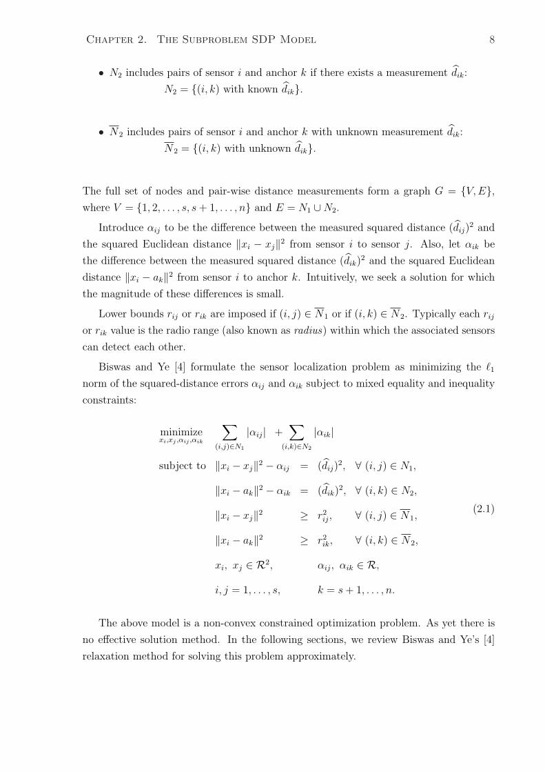
Biswas and Ye [4] formulate the sensor localization problem as minimizing the `1
norm of the squared-distance errors αij and αik subject to mixed equality and inequality
constraints:
minimizexi,xj ,αij ,αik
∑
(i,j)∈N1
|αij| +∑
(i,k)∈N2
|αik|
subject to ‖xi − xj‖2 − αij = (dij)2, ∀ (i, j) ∈ N1,
‖xi − ak‖2 − αik = (dik)2, ∀ (i, k) ∈ N2,
‖xi − xj‖2 ≥ r2ij, ∀ (i, j) ∈ N1,
‖xi − ak‖2 ≥ r2ik, ∀ (i, k) ∈ N2,
xi, xj ∈ R2, αij, αik ∈ R,
i, j = 1, . . . , s, k = s + 1, . . . , n.
(2.1)
The above model is a non-convex constrained optimization problem. As yet there is
no effective solution method. In the following sections, we review Biswas and Ye’s [4]
relaxation method for solving this problem approximately.
Chapter 2. The Subproblem SDP Model 9
2.2 The Euclidean Distance Model in Matrix Form
The distance model (2.1) is reformulated into (2.2) (refer to Biswas and Ye [4]) by intro-
ducing matrix variables as follows:
minimize∑
(i,j)∈N1
(α+ij + α−ij) +
∑
(i,k)∈N2
(α+ik + α−ik)
subject to eTij Y eij − α+
ij + α−ij = (dij)2, ∀ (i, j) ∈ N1,
(ei
−ak
)T(Y XT
X I
)(ei
−ak
)− α+
ik + α−ik = (dik)2, ∀ (i, k) ∈ N2,
eTij Y eij ≥ r2
ij, ∀ (i, j) ∈ N1,
(ei
−ak
)T(Y XT
X I
)(ei
−ak
)≥ r2
ik, ∀ (i, k) ∈ N2,
Y = XT X,
α+ij, α−ij, α+
ik, α−ik ≥ 0,
i, j = 1, . . . , s, k = s + 1, . . . , n,
(2.2)
where
• X = (x1 x2 . . . xs) is a 2× s matrix to be determined;
• eij is a zero column vector except for 1 in position i and −1 in position j, so that
‖xi − xj‖2 = eTij XT X eij;
• ei is a zero column vector except for 1 in position i, so that
‖xi − ak‖2 =
(ei
−ak
)T (X I
)T (X I
) (ei
−ak
);
• Y is defined to be XT X;
• The substitutions αij = α+ij − α−ij and αik = α+
ik − α−ik are made to deal with |αij|and |αik| in the normal way.
Chapter 2. The Subproblem SDP Model 10
2.3 The SDP Relaxation Model
The approach of Biswas and Ye [4] is to relax the constraint Y = XT X to be Y º XT X,
for which an equivalent matrix inequality is (Boyd et al. [6])
ZI ≡(
Y XT
X I
)º 0. (2.3)
With the definitions
AI =
0 0 0
1 0 1
0 1 1
, bI =
1
1
2
,
where 0 in AI is a zero column vector of dimension s, problem (2.2) is relaxed to a linear
SDP:
minimize∑
(i,j)∈N1
(α+ij + α−ij) +
∑
(i,k)∈N2
(α+ik + α−ik)
subject to diag(ATI Z AI) = bI ,
(eij
0
)T
Z
(eij
0
)− α+
ij + α−ij = (dij)2 ∀ (i, j) ∈ N1,
(ei
−ak
)T
Z
(ei
−ak
)− α+
ik + α−ik = (dik)2 ∀ (i, k) ∈ N2,
(eij
0
)T
Z
(eij
0
)≥ r2
ij ∀ (i, j) ∈ N1,
(ei
−ak
)T
Z
(ei
−ak
)≥ r2
ik ∀ (i, k) ∈ N2,
Z º 0, α+ij, α−ij, α+
ik, α−ik ≥ 0,
i, j = 1, . . . , s, k = s + 1, . . . , n,
(2.4)
where the constraint diag(ATI ZAI) = bI ensures that the matrix variable Z’s lower right
corner is a 2-dimensional identity matrix I, so that Z takes the form of ZI in (2.3).
Initially, Biswas and Ye [5, 4] omit the ≥ inequalities involving rij and rik, and solve
the resulting problem to obtain an initial solution Z1. (The inequality constraints increase
the problem size dramatically, and Z1 is likely to satisfy most of them.) They then adopt
Chapter 2. The Subproblem SDP Model 11
an “iterative active-constraint generation technique” in which inequalities violated by Zk
are added to the problem and the resulting SDP is solved to give Zk+1 (k = 1, 2, . . .).
The process usually terminates before all constraints are included. Further study of this
approach is presented in section 3.3.1.
2.4 SDP Model Analysis
Let Z =
(Y XT
X I
)
be a feasible solution of the relaxed SDP (2.4). Biswas and Ye [4]
give conditions under which X and Y solve problem (2.2) exactly, when exact distance
measurements are assumed:
• Z is the unique optimal solution of (2.4), including all inequality constraints.
• In (2.4), there are 2n + n(n + 1)/2 exact pair-wise distance measurements.
These conditions ensure that Y = XT X. In practice, distance measurements have
noise and we only know that the SDP solution satisfies Y − XT X º 0. This inequality
can be used for error analysis of the position estimation provided by the relaxation. For
example, trace(Y − XT X) =∑
τi, where
τi ≡ Yii − ‖xi‖2 ≥ 0, (2.5)
is a measure of deviation of the SDP solution from the desired constraint Y = XT X
(ignoring off-diagonal elements). The individual trace τi can be used to evaluate the
position estimation xi for sensor i. In particular, we interpret a smaller τi to mean higher
accuracy in the estimated position xi. Further explanation is given in [4].
Chapter 3
SpaseLoc: A Scalable Localization
Algorithm
When the number of nodes in (2.4) is large, applying a general SDP solver such as
DSDP5.0 [3] or SeDuMi [44] would not scale well. In this chapter, we present a sequential
subproblem approach named SpaseLoc to solve the full localization problem iteratively.
We first explain in detail how SpaseLoc works, followed by an example to illustrate
the steps of SpaseLoc. The last section presents computational results.
3.1 Adaptive Subproblem Approach
We call the overall sensor localization problem including all sensors and anchors the
full problem. At each iteration, SpaseLoc selects from the full problem a subset of the
unpositioned sensors and a subset of the anchors to form a localization subproblem. We
call the selected sensors in the subproblem subsensors, and the selected anchors in the
subproblem subanchors, These subsensors and subanchors, together with their known
distance measurements and known anchors’ locations, form a sub SDP relaxation model
to be solved using the same formulation as in (2.4).
In our adaptive approach, the subanchors and subsensors for each subproblem are
chosen dynamically according to rule sets. (Rather than using predefined data, every
new iteration’s subproblem generation is based on the previous iteration’s results.) The
resulting SDP subproblems are of varying but limited size. Currently they are solved by
Benson, Ye, and Zhang’s SDP solver DSDP5.0 [3].
SpaseLoc is a greedy algorithm in the sense that each subproblem determines the final
estimate of the associated sensor positions.
12
Chapter 3. SpaseLoc: A Scalable Localization Algorithm 13
3.1.1 The SpaseLoc Algorithm
The main steps of SpaseLoc are listed below, followed by explanations of the steps and
definitions of new terms used therein.
A0 Set subproblem size.
A1 Subproblem creation: Select subsensors and subanchors to be included in the sub-
problem.
A2 Formulate SDP relaxation model (2.4) based on the chosen subsensors and sub-
anchors, together with the known distances among them and the subanchors’ known
positions.
A3 Call SDP solver to obtain optimal solution for the subsensors’ positions.
A4 Classify positioned subsensors according to their τi value.
A5 If all sensors in the network become positioned or are determined to be outliers, go
to step A6. Otherwise, return to step A1 for the next iteration.
A6 Output all sensor locations and report outliers if any. Stop.
In step A0, subproblem size specifies a limit on the number of unpositioned sensors
to be included in each subproblem. It can range from 1 to a upper limit value that
is potentially solvable by the SDP solver. In our experiments, the upper limit is 150.
The most effective subproblem size seems to change with the full problem size, the model
parameters such as radius, and the SDP solver used. We perform an approximate line-
search to find subproblem size that corresponds to the minimum time, since empirically
the total execution time with all other parameters fixed is essentially a convex function
of subproblem size.
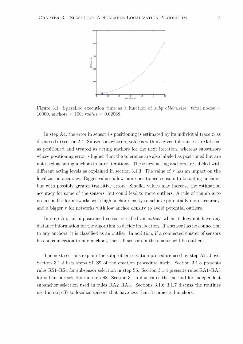
For example, when full problem size is 10000 with 100 anchors, radius 0.02068, and no
noise, subproblem size 5 seems to give the best execution time with the DSDP5.0 solver
(refer to Figure 3.1). The search time for subproblem size is not included as part of the
SpaseLoc execution time.
Step A1 involves choosing a subset of unpositioned sensors (no more than subprob-
lem size) and an associated subset of nodes with known positions. The latter can include
a subset of the original anchors and/or a subset of sensors already positioned by a pre-
vious subproblem (we define them as acting anchors). The rules for choosing subsensors
and subanchors in this iteration are discussed in sections 3.1.3–3.1.4.
Chapter 3. SpaseLoc: A Scalable Localization Algorithm 14
0 10 20 30 40 50 600
500
1000
1500
2000
2500
subproblem_size
CP
U s
econds
Figure 3.1: SpaseLoc execution time as a function of subproblem size: total nodes =10000, anchors = 100, radius = 0.02068.
In step A4, the error in sensor i’s positioning is estimated by its individual trace τi as
discussed in section 2.4. Subsensors whose τi value is within a given tolerance τ are labeled
as positioned and treated as acting anchors for the next iteration, whereas subsensors
whose positioning error is higher than the tolerance are also labeled as positioned but are
not used as acting anchors in later iterations. These new acting anchors are labeled with
different acting levels as explained in section 3.1.3. The value of τ has an impact on the
localization accuracy. Bigger values allow more positioned sensors to be acting anchors,
but with possibly greater transitive errors. Smaller values may increase the estimation
accuracy for some of the sensors, but could lead to more outliers. A rule of thumb is to
use a small τ for networks with high anchor density to achieve potentially more accuracy,
and a bigger τ for networks with low anchor density to avoid potential outliers.
In step A5, an unpositioned sensor is called an outlier when it does not have any
distance information for the algorithm to decide its location. If a sensor has no connection
to any anchors, it is classified as an outlier. In addition, if a connected cluster of sensors
has no connection to any anchors, then all sensors in the cluster will be outliers.
The next sections explain the subproblem creation procedure used by step A1 above.
Section 3.1.2 lists steps S1–S9 of the creation procedure itself. Section 3.1.3 presents
rules RS1–RS4 for subsensor selection in step S5. Section 3.1.4 presents rules RA1–RA3
for subanchor selection in step S8. Section 3.1.5 illustrates the method for independent
subanchor selection used in rules RA2–RA3. Sections 3.1.6–3.1.7 discuss the routines
used in step S7 to localize sensors that have less than 3 connected anchors.

Chapter 3. SpaseLoc: A Scalable Localization Algorithm 15
3.1.2 Subproblem Creation Procedure
As explained, subproblem size is a predetermined parameter that represents the maximum
number of unpositioned sensors that can be selected as subsensors in a subproblem.
When there are more than subproblem size unpositioned sensors, we have a choice to
make among them.
The subproblem creation procedure makes sure that the choice of subsensors is based
first on the number of connected anchors they have, and second on the type of connected
anchors such as original anchors and different levels of acting anchors as defined by
a priority list (section 3.1.3), and the choice of subanchors is based on a set of rules
(section 3.1.4). The main steps are listed below, followed by explanations of the steps
and definitions of new terms used.
S1 Specify MaxAnchorReq.
S2 Initialize AnchorReq = MaxAnchorReq.
S3 Loop through unpositioned sensors, finding all that are connected to at least An-
chorReq anchors. If AnchorReq ≥ 3, determine if there are 3 independent suban-
chors; if not, go to next sensor.1 Enter each found sensor into a candidate subsensor
list, and enter its connected anchors into a corresponding candidate subanchor list.
Each sensor in the candidate subsensor list has its own candidate subanchor list (so
there are as many candidate subanchor lists as the number of sensors in the candi-
date subsensor list). Let sub s candidate be the length of the candidate subsensor
list.
S4 If sub s candidate = subproblem size, the candidate subsensor list becomes the
chosen subsensors list. Go to step S8.
S5 If sub s candidate > subproblem size, the choice of subsensors is further based on
subsensor selection rules RS1–RS4 described in section 3.1.3. After exactly sub-
problem size subsensors are selected from the candidate list according these rules,
go to step S8.
S6 If sub s candidate < subproblem size and the candidate list is not null, go to step
S8.
1See section 3.1.5 for dependency definition and independent anchor selection.
Chapter 3. SpaseLoc: A Scalable Localization Algorithm 16
S7 Now sub s candidate = 0. Reduce AnchorReq by 1.
If AnchorReq ≥ 3, go to step S3 for another round of subproblem creation.
If AnchorReq = 2, apply the procedure in section 3.1.6 then go to step S3.
If AnchorReq = 1, apply the procedure in section 3.1.7 then go to step S3.
Otherwise, AnchorReq = 0 and sub s candidate = 0 indicates that there are still
unpositioned sensors left that are not connected to any positioned nodes. We
classify them as outliers and exit this procedure to continue at step A6 of section
3.1.1.
S8 Now that we have a subsensor list and the candidate subanchor lists, choose sub-
anchors using selection rules RA1–RA3 presented in section 3.1.4.
S9 The subsensors and subanchors are selected and the subproblem creation routine
finishes here. Continue at step A2 in section 3.1.1.
In step S1, MaxAnchorReq determines the initial (maximum) value of AnchorReq.
It is useful for scalability when connectivity is dense. A smaller MaxAnchorReq would
generally cause fewer subanchors to be included in the subproblem, thus reducing the
number of distance constraints in each SDP subproblem and hence reducing execution
time for each iteration. For instance, under ideal conditions (where there is no noise),
even if a sensor has 10 distance measurements to 10 anchors, we don’t need to include
all 10 anchors because we can use 3 to localize that sensor accurately.
In the presence of noise, a bigger MaxAnchorReq should reduce the average estimation
error. For example, if there is a large distance measurement error from one particular
anchor, since MaxAnchorReq anchors are all taken into consideration for deciding the
sensor’s actual position, the large error would be averaged out. Another consideration
for setting MaxAnchorReq is the trade-off between estimation accuracy and execution
speed. If we are in a static environment and would like to have sensor positioning as
accurate as possible under noise conditions, we might choose a large MaxAnchorReq.
However, in a real-time environment involving moving sensors, where speed might take
priority, we would consider a smaller MaxAnchorReq.
In step S2, AnchorReq is a dynamic parameter that may decrease in later steps.
In step S6, the subproblem will contain less than subproblem size subsensors, and
this is perfectly acceptable. The alternative is to reduce AnchorReq by 1 and find more
subsensor candidates that have fewer distance connections. However, this approach might
reduce the accuracy of the algorithm, because we do want to localize the subsensors as

Chapter 3. SpaseLoc: A Scalable Localization Algorithm 17
accurately as possible as the iteration progresses, and the newly localized subsensors
could be further used as acting anchors for the next iteration.
In step S7, AnchorReq is iteratively reduced by 1 from MaxAnchorReq to 0 eventually.
This approach allows sensors with at least AnchorReq connections to anchors to be
positioned before sensors with fewer connections to anchors. As we know, under no-noise
conditions, a sensor’s position can be uniquely determined by at least 3 independent
distance measurements to 3 anchors. If a sensor has only 2 distance measurements to
2 anchors, there are two possible locations; and if there is only 1 distance measurement
to an anchor, the sensor can be anywhere on a circle. In this situation, we use heuristic
subroutines described in sections 3.1.6–3.1.7 to include the sensor’s anchors’ connected
neighboring nodes in the subproblem in order to improve the estimation accuracy.
3.1.3 Subsensor Selection Priority List
In step S5, when the number of sensors in the candidate subsensor list is bigger than
subproblem size, the choice of subsensors is further based on the types of anchors each
sensor is connected to.
First, we introduce the concept of sensor priority. We assign a priority to each sensor
in the candidate subsensor list. A sensor with a smaller priority value is selected to be
localized before one with a bigger priority value. A sensor’s priority is based on the types
of anchors the sensor is directly connected to. Next, in order to define different types of
anchors, we introduce the concept of anchor acting levels. All anchors including acting
anchors are assigned certain acting levels. Original anchors are always set to acting
level 1. Every acting anchor is set to an acting level after it has been localized as a
sensor. The acting level depends on the priority of the sensor that becomes this acting
anchor. Essentially, acting anchors are set with acting levels depending on the levels of
the anchors that localized them.
The priority rules for selecting subsensors from a candidate subsensor list are as
follows:
RS1 When AnchorReq ≥ 3 and a sensor has at least 3 connected anchors that are
independent, the sensor’s priority depends on the lowest acting level among all the
connected anchors and the number of anchors in this level. The lower the acting
level and the larger the number of anchors in that level, the higher the sensor’s
priority.
RS2 If the sensor has 3 connected anchors that are dependent, it is ranked with the
same priority as when the sensor is connected to only 2 anchors.
Chapter 3. SpaseLoc: A Scalable Localization Algorithm 18
Table 3.1: An example: priority list when MaxAnchorReq=3.
Priority Level 1 Level 2 Level 3–7 Level 8–10 Resulting
value anchor anchor anchor anchor level1 ≥ 3 any any any 22 = 2 total ≥ 1 any 33 = 1 total ≥ 2 any 44 0 ≥ 3 any any 55 0 = 2 total ≥ 1 any 66 0 ≤ 1 total ≥ 2 if level 2 anchor = 1, else total ≥ 3 any 77 total ≥ 3, at least one of the 3 anchors is acting level 8 or 9, or 10 88 total = 2 99 total = 1 10
RS3 Sensors with 2 anchor connections are ranked with equal priority, independent of
the acting levels of the 2 connected anchors. (This can be easily expanded to
be more granular according to the connected anchors’ acting levels.) Sensors in
this category are assigned lower priority than any sensors that have at least 3
independent anchor connections.
RS4 Sensors with 1 anchor connection are ranked with equal priority, independent of the
acting level of the connected anchor. (Again, this can be more granular according
to the connected anchor’s acting level.) Sensors in this category are assigned lower
priority than any sensors that have at least 2 anchor connections.
Table 3.1 illustrates the priority list for an example where MaxAnchorReq = 3 and
the sensor’s priority is determined by the number of its connected anchors that have
the lowest acting level among all the sensor’s connected anchors. We can certainly add
more granularity by further classifying the sensor’s second and third connected anchors’
acting levels. Although more categorizations of the priorities should increase localization
accuracy under most noise conditions, more computational effort is required to handle
more levels of priorities. In Table 3.1, we assume we will generate only 9 levels of
priorities.
Each item in the table represents the number of anchors with different acting levels
that is needed at each priority. The last column represents the resulting acting anchors’
acting levels for subsequent iterations. For example, if a sensor has at least three inde-
pendent connections to anchors, and if 2 of the anchors are original anchors (acting level
1) and at least 1 of the connected anchors is at any acting level from 2 to 7, this sensor
belongs to priority 2 as listed in row 2 of the table. Also, when this sensor is positioned,
Chapter 3. SpaseLoc: A Scalable Localization Algorithm 19
it becomes acting anchor level 3. The sensors that connect to two anchors belong to
the second last priority (8 in the table), and sensors that connect to only one anchor
belong to the last priority (9 in this case). In addition, if a sensor connects to at least 3
independent anchors, among which at least one anchor belongs to level 8, 9, or 10, this
sensor will be classified as the third last priority as listed in row 7.
3.1.4 Subanchors Selection
In step S8, for each unpositioned subsensor, only AnchorReq of the connected anchors are
allowed to be included in the subproblem. We use the following rules to select subanchors
from a candidate subanchor list that contains more than AnchorReq anchors.
RA1 Original anchors are selected first, followed by acting anchors with lower acting
level.
RA2 The subanchors chosen should be linearly independent.
RA3 Among independent anchors in the candidate subanchor list, we use distance scale-
factors to encourage selection of the closest subanchors.
Rules RA2 and RA3 are implemented as in section 3.1.5. Rule RA3 is based on
the assumption that under noise conditions, we trust the shorter distance measurements
more than the longer ones. This is specially true for ranging devices based on RF (radio
frequency) strength.
For certain applications, it may be beneficial to choose MaxAnchorReq large in order
to increase the localization accuracy, though it could impact the algorithm speed.
3.1.5 Independent Subanchors Selection
Suppose sensor i is connected to K (K >3) anchors at locations aik with corresponding
distance measurements dik (k = 1, . . . , K). Define the matrices
A =
(1 1 . . . 1
−ai1 −ai2 . . . −aiK
), D1 = diag(1/
√1 + ‖aik‖2), D2 = diag(1/dik).
We select an independent subset by a QR factorization with column interchanges [17]:
B = AD1D2, BP = QR, where Q is orthogonal, R is upper-trapezoidal, and P is a
permutation chosen to maximize the next diagonal of R at each stage of the factorization.
(D1 normalizes the columns of A, and D2 biases them in favor of anchors that are closer
Chapter 3. SpaseLoc: A Scalable Localization Algorithm 20
to sensor i.) If the 3rd diagonal of R is larger than a predefined threshold (10−4 is
used in our simulation), the first 3 columns of AP are regarded as independent, and
the associated anchors are chosen. Otherwise, all subsets of 3 among the K anchors are
regarded as dependent. (In Matlab, R and P are obtained by a command of the form
[Q,R,P] = qr(B).)
3.1.6 Geometric Subroutine (Two Connected Anchors)
This section illustrates the heuristic techniques used in step S7 of section 3.1.2 to localize
sensors connected to only two anchors.
When a sensor’s connected anchors are also connected to other anchors, this subrou-
tine may improve the accuracy of the sensor’s positioning, as illustrated by an example
in Figure 3.2.
±°²¯s1 ±°
²¯a3
±°²¯a4 ±°
²¯a5
±°²¯a6 ±°
²¯a7 ±°
²¯s2
(0, 0) (1, 0) (2, 0) (3, 0) (4, 0) (5, 0)b
(6, 0)
(0, 1)
(0, 2)
(2, 3)b
(5, 2)b
Figure 3.2: Sensors with connections to at most two anchors.
In this example, assume s1 and s2 are sensors with unknown locations, and a3(1, 3),
a4(1, 2), a5(2, 2), a6(4, 1), a7(5, 1) are anchors with known positions in brackets. Assume
that the sensors’ radio range is√
2, and we are also given two distance measurements
d13 = 1 and d14 =√
2 for sensor s1 and one measurement d27 = 1 for sensor s2.
Given two distances d13 and d14 to two anchors a3(1, 3) and a4(1, 2), we know that
s1 should be either at (0, 3) or (2, 3). If we only use s1, a3(1, 3), a4(1, 2) in an SDP
subproblem, SDP relaxation will give a solution near the middle of the two possible
points, which would be very close to point (1, 3). If there is any anchor (a5) that is near
s1’s connected anchors (a3 and a4) with any of the two possible sensor’ points within
their radio range (point (2, 3) is within a5’s range), that point (2, 3) must not be the real
location of s1, or else s1 would be connected to this anchor (a5) as well. Thus we can
infer that s1 must be at the other point (0, 3).
Inspired by the above observation, when a sensor has at most 2 connected anchors, we
include these anchors’ connected anchors in the subproblem (we call them the connected
Chapter 3. SpaseLoc: A Scalable Localization Algorithm 21
&%
'$aal
ÁÀ
¿a
a2
"!
#Ãaa3a
x
kaa2&%
'$aa3
ax µ´¶³
aa2
&%
'$a
a3
ax
(a) (b) (c)
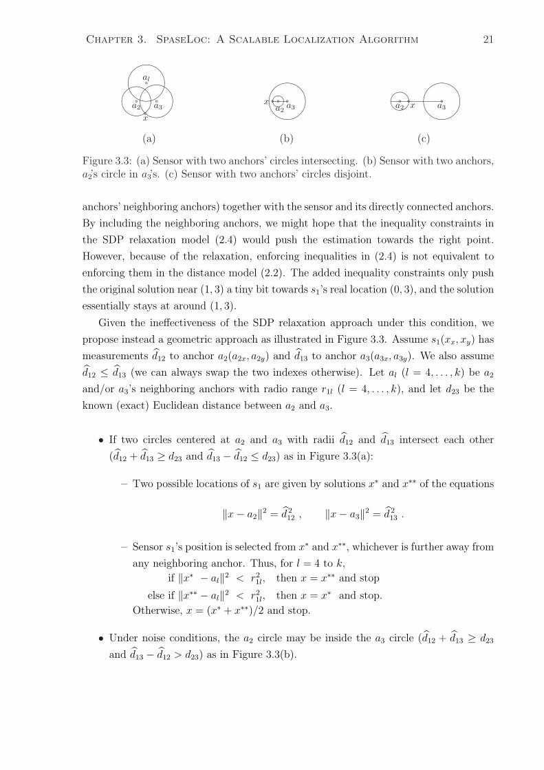
Figure 3.3: (a) Sensor with two anchors’ circles intersecting. (b) Sensor with two anchors,a2’s circle in a3’s. (c) Sensor with two anchors’ circles disjoint.
anchors’ neighboring anchors) together with the sensor and its directly connected anchors.
By including the neighboring anchors, we might hope that the inequality constraints in
the SDP relaxation model (2.4) would push the estimation towards the right point.
However, because of the relaxation, enforcing inequalities in (2.4) is not equivalent to
enforcing them in the distance model (2.2). The added inequality constraints only push
the original solution near (1, 3) a tiny bit towards s1’s real location (0, 3), and the solution
essentially stays at around (1, 3).
Given the ineffectiveness of the SDP relaxation approach under this condition, we
propose instead a geometric approach as illustrated in Figure 3.3. Assume s1(xx, xy) has
measurements d12 to anchor a2(a2x, a2y) and d13 to anchor a3(a3x, a3y). We also assume
d12 ≤ d13 (we can always swap the two indexes otherwise). Let al (l = 4, . . . , k) be a2
and/or a3’s neighboring anchors with radio range r1l (l = 4, . . . , k), and let d23 be the
known (exact) Euclidean distance between a2 and a3.
• If two circles centered at a2 and a3 with radii d12 and d13 intersect each other
(d12 + d13 ≥ d23 and d13 − d12 ≤ d23) as in Figure 3.3(a):
– Two possible locations of s1 are given by solutions x∗ and x∗∗ of the equations
‖x− a2‖2 = d 212 , ‖x− a3‖2 = d 2
13 .
– Sensor s1’s position is selected from x∗ and x∗∗, whichever is further away from
any neighboring anchor. Thus, for l = 4 to k,
if ‖x∗ − al‖2 < r21l, then x = x∗∗ and stop
else if ‖x∗∗ − al‖2 < r21l, then x = x∗ and stop.
Otherwise, x = (x∗ + x∗∗)/2 and stop.
• Under noise conditions, the a2 circle may be inside the a3 circle (d12 + d13 ≥ d23
and d13 − d12 > d23) as in Figure 3.3(b).
Chapter 3. SpaseLoc: A Scalable Localization Algorithm 22
– The solutions x∗ and x∗∗ of the following equations give two possible points
for s1 on the a2 circle:
(xx − a2x)2 + (xy − a2y)
2 = d 212,
(a2x − a3x)(xy − a2y) = (a2y − a3y)(xx − a2x),
where x is on the line through a2 and a3 represented by the second equation.
– If ‖x∗ − a3‖ < ‖x∗∗ − a3‖, then x = x∗∗; otherwise x = x∗. This guarantees
that the point further from a3 is chosen. Note that we base the sensor’s
estimation on the closest anchor (a2 here since d13 ≥ d12), assuming that a
shorter measurement is generally more accurate than longer ones, given similar
anchor properties.
The same approach applies when the a3 circle is inside the a2 circle (d12−d13 > d23).
• Under noise conditions, the a2 and a3 circles may again have no intersection (d12 +
d13 < d23) as in Figure 3.3(c).
– The solutions x∗ and x∗∗ of the following equations give two possible points
for s1 on the circle for the anchor with smaller radius. Let’s assume d12 ≤ d13:
(xx − a2x)2 + (xy − a2y)
2 = d 212,
(a2x − a3x)(xy − a2y) = (a2y − a3y)(xx − a2x),
where x is on the line through a2 and a3 represented by the second equation.
– If ‖x∗ − a3‖ > ‖x∗∗ − a3‖, then x = x∗∗; otherwise x = x∗. This guarantees
that the point closer to a3 (in between a2 and a3) is chosen.
3.1.7 Geometric Subroutine (One Connected Anchor)
Similar inefficiency occurs in the SDP solution when a sensor connects to only one anchor.
The SDP solver under this condition gives a solution for the sensor to be in the same
location as the sensor’s connected anchor. In reality, the sensor could be anywhere on
the circle. The SDP gives an average point, at the center of the circle, and that is where
the connected anchor is. Even if the anchor’s neighboring anchor is included in the SDP
subproblem, the inequality constraints are not active most of the time because the SDP
solution may not provide optimal solutions all the time.
Chapter 3. SpaseLoc: A Scalable Localization Algorithm 23
&%
'$a
b ÁÀ
¿aa
ax∗
&%
'$ab
ÁÀ
¿aa ax∗
&%
'$ac
1
23 4
(a) (b)
Figure 3.4: (a) Sensor with one anchor connection a and one neighboring anchor b. (b)Sensor with one anchor connection a and two neighboring anchors b, c.
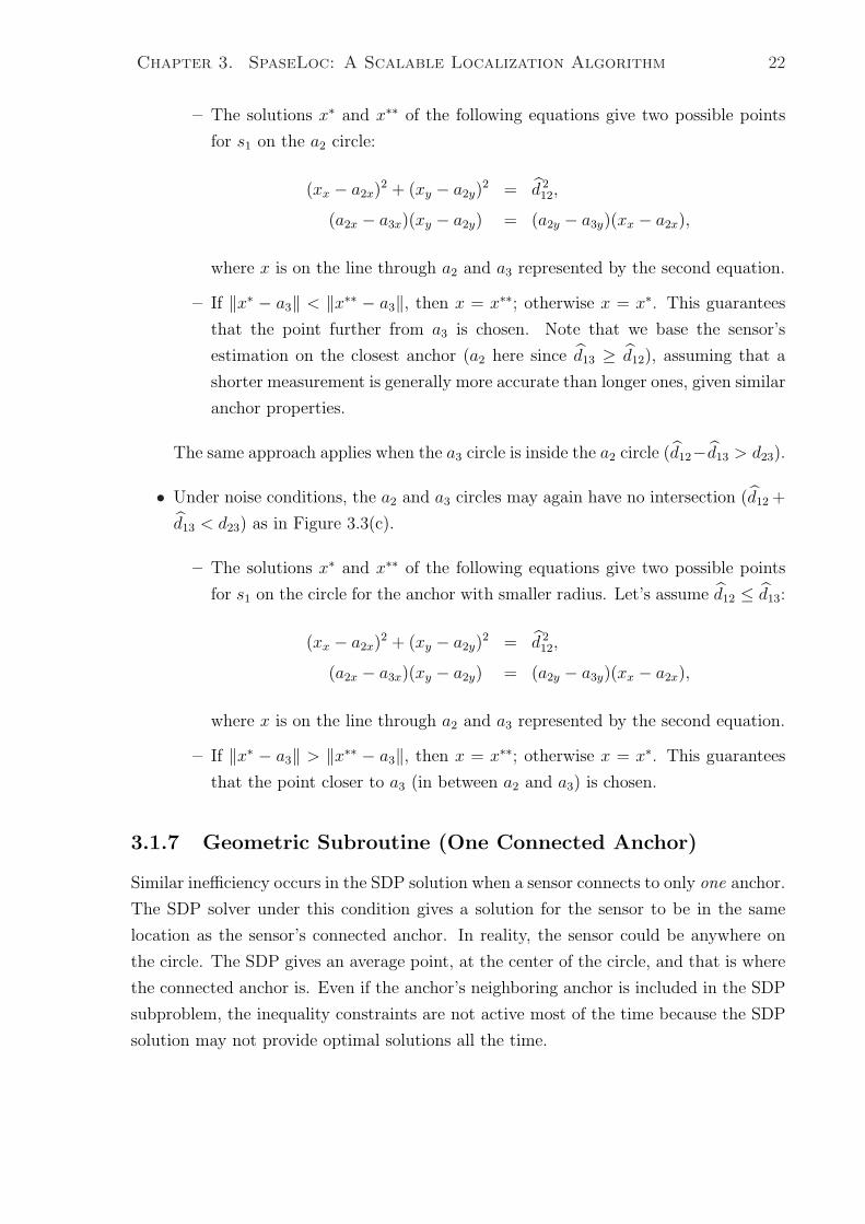
We propose a heuristic for estimating a sensor’s location with only one connecting
anchor. The idea is to use one neighboring anchor’s radio range information to eliminate
the portion of the circle that the sensor would not be on, and then calculate the middle of
the other portion of the circle to be the sensor’s position. For the example in Figure 3.2,
because we know the distance between s2 and a7 is 1, we know that s2 could be anywhere
on the circle surrounding a7 with a radius of 1. Knowing a7’s neighboring anchor node
a6 is not connected to s2, we know that s2 would not be in the area surrounding a6 with
a radius of√
2. Thus, s2 could be anywhere around the half circle including points (5, 2),
(6, 1), (5, 0). The heuristic chooses the middle point between the two circles’ intersection
points (5, 2) and (5, 0), which happens to be (6, 1) in this example. The heuristic gives
better accuracy for the sensor’s location than the SDP solution under most conditions.
The procedure follows:
• Assume s has one distance measurement d to anchor a, and b is the closest connected
neighboring anchor to a with radio range r (refer to Figure 3.4(a)). We assume
a = (ax, ay), b = (bx, by), x = (xx, xy).
• The solutions x∗ and x∗∗ of the following equations give two possible points s on
the circle:
(xx − ax)2 + (xy − ay)
2 = d 2,
(ax − bx)(xy − ay) = (ay − by)(xx − ax),
where x is on the line through a and b represented by the second equation.
• If ‖x∗ − b‖ < r, then x = x∗∗; otherwise x = x∗. This guarantees that the point
further from b is chosen.
The above heuristic provides a simple way of estimating a sensor’s location when
the sensor connects to only one anchor. A more complicated approach can be adopted
Chapter 3. SpaseLoc: A Scalable Localization Algorithm 24
when the connected anchor has more than one neighboring anchor, which can increase
the accuracy of the sensor’s location. We call it an arc elimination heuristic. The idea
is to loop through each of the neighboring anchors and find the portion of the circle
that the sensor won’t be on, and eliminate that arc as a possible location of the sensor.
Eventually, when one or more plausible arcs remain, we choose the middle of the largest
arc to be the sensor’s location. For example, assume we add one more neighboring anchor
c to sensor s’s anchor a from the previous example in Figure 3.4(a). The new scenario is
shown in Figure 3.4(b). First, we find the intersections (points 1 and 2) of two circles:
one at a with radius d, the other at b with radius r. We know that the 1–2 portion of the
arc closer to point b won’t be the location of s. Second, we find the intersections (points
3 and 4) of two circles: one at a with radius d, the other at c with radius r. We know
that the arc 3–4 closer to point c won’t be the location of s. Thus we deduce that s must
be somewhere on the arc 1–4 further away from b or c. The estimation of s is given in
the middle of the arc 1–4. As we see, this method should provide more accuracy than
the one-neighboring-anchor approach.
3.2 An Example
A simple example is shown in Figure 3.5 to illustrate the SpaseLoc algorithm and some
of the rules of the subproblem selection process. Assume s1, s2, . . . , s14 are sensors with
unknown locations, and a15, a16, . . . , a20 are original anchors. Assume that the actual
locations of these nodes are all on a regular square grid structure with edge size 1, and
that the sensors’ radio range is√
2. We also use the priority list in Table 3.1 in this
example.
±°²¯a15 ±°
²¯s1 ±°
²¯s2 ±°
²¯s3 ±°
²¯s10 ±°
²¯s11
±°²¯a16 ±°
²¯s4 ±°
²¯s5 ±°
²¯s6
±°²¯a17 ±°
²¯s7 ±°
²¯s8 ±°
²¯s9 ±°
²¯s12 ±°
²¯s13
±°²¯a18 ±°
²¯a19 ±°
²¯s14 ±°
²¯a20
Figure 3.5: An example.
• In A0 we set subproblem size = 3.
Chapter 3. SpaseLoc: A Scalable Localization Algorithm 25
• In A1 we go through the subproblem creation procedure:
– In S1 we set MaxAnchorReq = 3
– In S2, AnchorReq is set to MaxAnchorReq, which is 3.
– S3 goes through the unpositioned sensor list and finds that s4 and s7 both have
at least 3 connections to anchors. However, anchors a15, a16, a17 connected
to sensor s4 are dependent, so the subsensor candidate list is only s7 for this
iteration.
– Since the subsensor candidate list of 1 is shorter than the subproblem size of
3, we are at S6. AnchorReq is not reduced yet because the candidate list is
not empty. Continue to S8.
– In S8, we have anchors a16, a17, a18, a19 connected to sensor s7 in the subsensor
candidate list, so we follow the subanchor selection rules RA1–RA3 in section
3.1.4. Rule RA2 says to choose three independent anchors, which could be a16,
a18, a19 or a17, a18, a19. Since anchors a16, a17, a18 are dependent, they won’t
be chosen. Rule RA3 says that if there are multiple anchors to choose from,
the closest ones should be used. Therefore a17, a18, a19 are selected instead of
a16, a18, a19.
– In S9, the subproblem consists of subsensor s7 and subanchors a17, a18, a19.
• In A2, formulate the SDP subproblem from subsensor s7 and subanchors a17, a18,
a19.
• In A3, call SDP to give s7’s position estimation.
• In A4, s7 is positioned and becomes an acting anchor at level 2 for the next iteration.
• In A5, some sensors are still not positioned. Go back to A1.
• With s7 as acting anchor, iterate steps A1–A5 (2nd time). s4, s8, s14 are positioned
in this iteration with subanchors a16, a17, a19, a20, s7, and all become acting anchors
at level 3 for the next iteration.
• With added acting anchors s4, s8, s14, iterate steps A1–A5 (3rd time). s1, s5, s9 are
positioned with subanchors a15, a16, s4, s7, s8, s14, a20, and become acting anchors
at levels 3, 7, 4.
Chapter 3. SpaseLoc: A Scalable Localization Algorithm 26
• With added acting anchors s5 and s9, iterate steps A1–A5 (4th time). s2 and s6
are positioned with subanchors s1, s4, s5, s8, s9, and both become acting anchors
at level 7.
• With added acting anchors s2 and s6, iterate steps A1–A5 (5th time). s3 is posi-
tioned with subanchors s2, s5, s6, and becomes acting anchor at level 7.
• With s3 positioned, iterate steps A1–A5 (6th time). Although we find unpositioned
sensor s12 has connections to 3 anchors s6, s9, a20, they are dependent. There is
no unpositioned sensor with connections to at least 3 independent anchors, so we
move to S7.
• Since the subsensor candidate list is now empty, AnchorReq is reduced from 3
to 2 at S7. Iterate steps A1–A5 (7th time) with a new AnchorReq value of 2,
finding s12 and s10 with at least 2 anchor connections. Since s12 has connections
to 3 dependent anchors s6, s9, a20, it is effectively the same as being connected
to exactly 2 anchors. s10 is connected to s3 and s6. We now follow the geometric
subroutine in section 3.1.6 for sensors connected to two anchors. Subanchors s3,
s6, s8, a20 have connected neighboring anchors s2, s5, s8, s14 and they are used to
exclude the other possible points for s10 and s12. Thus s10 is now positioned, and
both become acting level 9.
• With s10 positioned, iterate steps A1–A5 (8th time). There is no unpositioned
sensor with connections to at least 2 anchors, so we move to S7 again.
• Since the subsensor candidate list is now empty, AnchorReq is further reduced from
2 to 1 at S7. Iterate steps A1–A5 (9th time) with a new AnchorReq value of 1.
Since s11 connects to only one subanchor s10, follow the geometric subroutine in
section 3.1.7. s10’s nearest connected neighboring anchor s3 is used to determine
the position of s11, and it becomes acting level 10.
• Iterate steps A1–A5 (10th time). There is no unpositioned sensor with connections
to 1 or more anchors, so we move to S7 again.
• Since the subsensor candidate list is now empty, AnchorReq is further reduced from
1 to 0 at S7. Because AnchorReq = 0 and there is one more unpositioned sensor
s13, s13 is classified as an outlier in S7. Now we move to step A6.
• In A6, report sensor positions and outliers and stop.
Chapter 3. SpaseLoc: A Scalable Localization Algorithm 27
3.3 Computational Results
This section explains the simulation method and the setup for experimenting with the
SpaseLoc algorithm, then presents results for various parameter settings.
For the simulation, a total number of nodes n (including s sensors and m anchors)
is specified in the range 50 to 10000. The positions of these nodes are assigned with a
uniform random distribution on a square region of size r × r where r = 1, or put on
the grid points of a regular topology such as a square or an equilateral triangle on the
same region. MaxAnchorReq = 3 is used in the simulation. The m anchors are randomly
chosen from the given n nodes. We assume all sensors have the same radio range (radius)
for any given test case. Various radio ranges were tested in the simulation.
Euclidean distances dij = ‖xi − xj‖ are calculated among all sensor pairs (i, j) for
i < j. We then use dij to simulate measured distances, where dij is dij times a random
error simulated by noise factor ∈ [0, 1]. For a given radius ⊆ [0, 1] it is defined as follows:
• If dij ≤ radius, then dij = dij(1+rn∗noise factor), where rn is normally distributed
with mean zero and variance one. (Any numbers generated outside (−1, 1) are
regenerated.)
In practical networks, depending on the technologies that are being used to obtain
the distance measurements, there may be many factors that contribute to the noise
level. For example, one way to obtain the distance measurement is to use the
received radio signal strength between two sensors. The signal strength could be
affected by media or obstacles in between the two sensors. In this study, noise factor
is a normally distributed random variable with mean zero and variance one. This
model could be replaced by any other noise model in practice.
• If dij > radius, the bound rij = 1.001 ∗ radius is used in the SDP model.
In the simulation, we define the average estimation error to be 1s
∑si=1 ‖xi − xi‖, where
xi is from the SDP solution and xi is the ith node’s true position. In a practical setting,
we wouldn’t know the node’s true location xi. Instead, we would use the node’s trace τi
(2.5) to gauge the estimation error.
To convey the distribution of estimation errors and trace, we also give the 95% quar-
tile.
Factors such as noise level, radio range, and anchor densities can directly impact
localization accuracy. The sensors’ estimated positions are derived directly from the given
distance measurements. If the noise level in these measurements is high, the estimation
accuracy cannot be high. We also need sufficiently large radio range to achieve accurate
Chapter 3. SpaseLoc: A Scalable Localization Algorithm 28
positioning, because too small a range could cause many sensors to be unreachable.
Finally, more anchors in the network should help with the estimation accuracy because
there are more reference points.
In the following subsections, we present simulation results (most results averaged over
10 runs) to show the accuracy and scalability of the SpaseLoc algorithm. We observe the
impact of various radio ranges, anchor densities, and noise levels on the accuracy and
performance of the algorithm. Computations were performed on a laptop computer with
2.4GHz CPU and 1GB system memory, using Matlab 6.5 [29] for SpaseLoc and a Mex
interface to DSDP5.0 (Benson, Ye, and Zhang [3]) for the SDP solutions.
3.3.1 Effect of Inequality Constraints in SDP Relaxation Model
As we discussed in section 3.1.6, because of the Y º XT X constraint relaxation, enforcing
the r2ij and r2
ik inequality constraints in (2.4) is not equivalent to enforcing them in the
distance model (2.2). In order to observe the effectiveness of including these inequality
constraints, we conduct simulations with the following three strategies, according to the
number of times we check for violated inequality constraints and then include them to
obtain new solution.
I2 corresponds to solving the SDP problem with all equalities (and no inequalities),
and then adding violated inequality constraints and re-solving one or more times
until all inequalities are satisfied. The final solution is an optimal solution to
problem (2.4).
I1 corresponds to solving the SDP problem with all equalities and then adding all
violated inequality constraints at most once.
I0 corresponds to solving the SDP problem with equality constraints only. (No in-
equality constraints are ever added.) The final solution is optimal for problem
(2.4) without the inequality constraints involving r2ij and r2
ik.
Our experimental results show that the added inequality constraints do not always
provide better positioning accuracy, but greatly increase the execution time. In this
section, we illustrate the inequality constraints’ impact through two simulation examples:
one with no noise but low connectivity; the other with full connectivity but with noise.
In our first example, we run simulation results on a network of 100 randomly uniform-
distributed sensors with radius 0.2275 and 10 randomly selected anchors. One of the
sensors happens to be connected to only two other nodes. The sensors are localized with
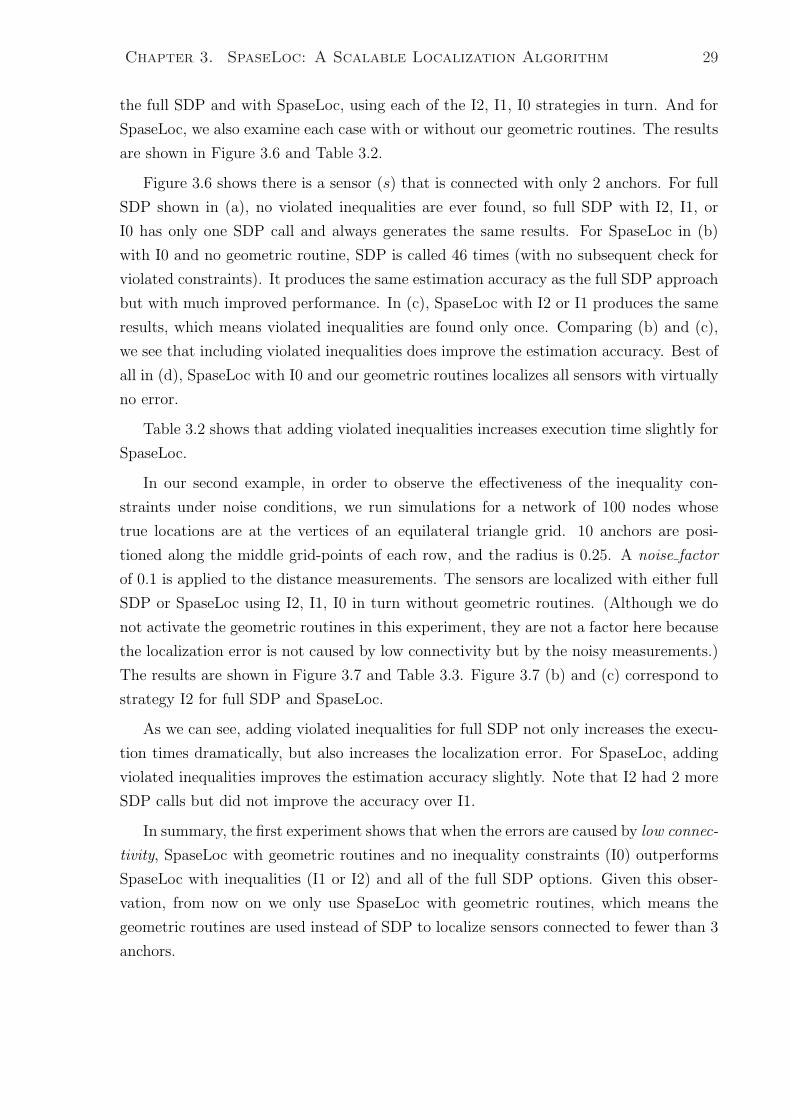
Chapter 3. SpaseLoc: A Scalable Localization Algorithm 29
the full SDP and with SpaseLoc, using each of the I2, I1, I0 strategies in turn. And for
SpaseLoc, we also examine each case with or without our geometric routines. The results
are shown in Figure 3.6 and Table 3.2.
Figure 3.6 shows there is a sensor (s) that is connected with only 2 anchors. For full
SDP shown in (a), no violated inequalities are ever found, so full SDP with I2, I1, or
I0 has only one SDP call and always generates the same results. For SpaseLoc in (b)
with I0 and no geometric routine, SDP is called 46 times (with no subsequent check for
violated constraints). It produces the same estimation accuracy as the full SDP approach
but with much improved performance. In (c), SpaseLoc with I2 or I1 produces the same
results, which means violated inequalities are found only once. Comparing (b) and (c),
we see that including violated inequalities does improve the estimation accuracy. Best of
all in (d), SpaseLoc with I0 and our geometric routines localizes all sensors with virtually
no error.
Table 3.2 shows that adding violated inequalities increases execution time slightly for
SpaseLoc.
In our second example, in order to observe the effectiveness of the inequality con-
straints under noise conditions, we run simulations for a network of 100 nodes whose
true locations are at the vertices of an equilateral triangle grid. 10 anchors are posi-
tioned along the middle grid-points of each row, and the radius is 0.25. A noise factor
of 0.1 is applied to the distance measurements. The sensors are localized with either full
SDP or SpaseLoc using I2, I1, I0 in turn without geometric routines. (Although we do
not activate the geometric routines in this experiment, they are not a factor here because
the localization error is not caused by low connectivity but by the noisy measurements.)
The results are shown in Figure 3.7 and Table 3.3. Figure 3.7 (b) and (c) correspond to
strategy I2 for full SDP and SpaseLoc.
As we can see, adding violated inequalities for full SDP not only increases the execu-
tion times dramatically, but also increases the localization error. For SpaseLoc, adding
violated inequalities improves the estimation accuracy slightly. Note that I2 had 2 more
SDP calls but did not improve the accuracy over I1.
In summary, the first experiment shows that when the errors are caused by low connec-
tivity, SpaseLoc with geometric routines and no inequality constraints (I0) outperforms
SpaseLoc with inequalities (I1 or I2) and all of the full SDP options. Given this obser-
vation, from now on we only use SpaseLoc with geometric routines, which means the
geometric routines are used instead of SDP to localize sensors connected to fewer than 3
anchors.
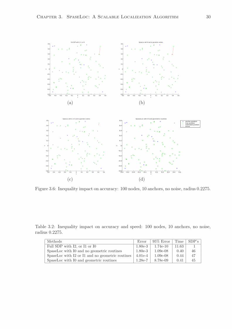
Chapter 3. SpaseLoc: A Scalable Localization Algorithm 30
−0.5 −0.4 −0.3 −0.2 −0.1 0 0.1 0.2 0.3 0.4 0.5−0.5
−0.4
−0.3
−0.2
−0.1
0
0.1
0.2
0.3
0.4
0.5
x
y
Full SDP with I2, I1, or I0
−0.5 −0.4 −0.3 −0.2 −0.1 0 0.1 0.2 0.3 0.4 0.5−0.5
−0.4
−0.3
−0.2
−0.1
0
0.1
0.2
0.3
0.4
0.5
x
y
SpaseLoc with I0 and no geometric routines
(a) (b)
−0.5 −0.4 −0.3 −0.2 −0.1 0 0.1 0.2 0.3 0.4 0.5−0.5
−0.4
−0.3
−0.2
−0.1
0
0.1
0.2
0.3
0.4
0.5
x
y
SpaseLoc with I2, or I1 and no geometric routines
−0.5 −0.4 −0.3 −0.2 −0.1 0 0.1 0.2 0.3 0.4 0.5−0.5
−0.4
−0.3
−0.2
−0.1
0
0.1
0.2
0.3
0.4
0.5
x
ySpaseLoc with I0 and geometric routines
anchor positiontrue positionestimated positionerrors
(c) (d)
Figure 3.6: Inequality impact on accuracy: 100 nodes, 10 anchors, no noise, radius 0.2275.
Table 3.2: Inequality impact on accuracy and speed: 100 nodes, 10 anchors, no noise,radius 0.2275.
Methods Error 95% Error Time SDP’sFull SDP with I2, or I1 or I0 1.80e-3 1.74e-10 11.63 1SpaseLoc with I0 and no geometric routines 1.80e-3 1.09e-08 0.40 46SpaseLoc with I2 or I1 and no geometric routines 4.01e-4 1.09e-08 0.44 47SpaseLoc with I0 and geometric routines 1.28e-7 8.78e-09 0.41 45
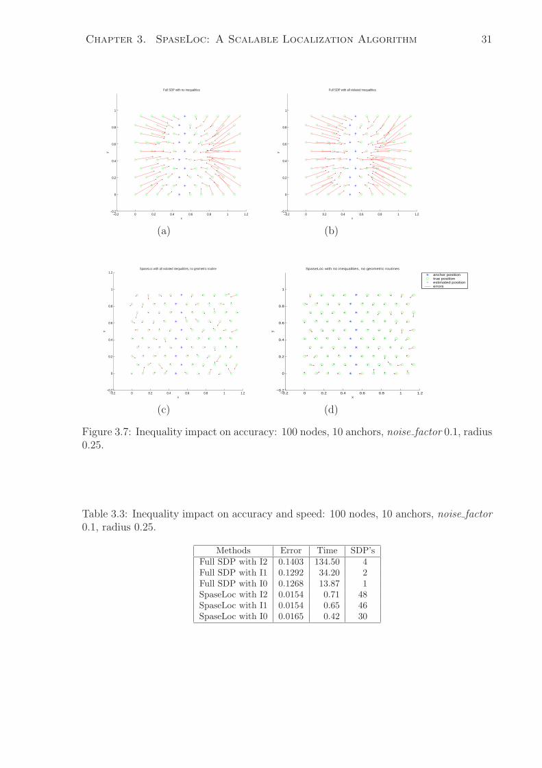
Chapter 3. SpaseLoc: A Scalable Localization Algorithm 31
−0.2 0 0.2 0.4 0.6 0.8 1 1.2−0.2
0
0.2
0.4
0.6
0.8
1
x
y
Full SDP with no inequalities
−0.2 0 0.2 0.4 0.6 0.8 1 1.2−0.2
0
0.2
0.4
0.6
0.8
1
x
y
Full SDP with all violated inequalities
(a) (b)
−0.2 0 0.2 0.4 0.6 0.8 1 1.2−0.2
0
0.2
0.4
0.6
0.8
1
1.2
x
y
SpaseLoc with all violated inequalities, no geometric routine
−0.2 0 0.2 0.4 0.6 0.8 1 1.2−0.2
0
0.2
0.4
0.6
0.8
1
x
ySpaseLoc with no inequalities, no geometric routines
anchor positiontrue positionestimated positionerrors
(c) (d)
Figure 3.7: Inequality impact on accuracy: 100 nodes, 10 anchors, noise factor 0.1, radius0.25.
Table 3.3: Inequality impact on accuracy and speed: 100 nodes, 10 anchors, noise factor0.1, radius 0.25.
Methods Error Time SDP’sFull SDP with I2 0.1403 134.50 4Full SDP with I1 0.1292 34.20 2Full SDP with I0 0.1268 13.87 1SpaseLoc with I2 0.0154 0.71 48SpaseLoc with I1 0.0154 0.65 46SpaseLoc with I0 0.0165 0.42 30
Chapter 3. SpaseLoc: A Scalable Localization Algorithm 32
The second experiment indicates that under noise conditions, although adding vio-
lated inequalities does not seem to improve the estimation accuracy for full SDP, it does
improve accuracy for SpaseLoc.
In the subsequent sections, we continue to examine the inequality constraints’ effects
on accuracy and speed.
3.3.2 Accuracy and Speed Comparison: Full SDP vs SpaseLoc
For very small networks, the full SDP solution is both accurate and efficient. (This is
vital to the performance of SpaseLoc, as many small subproblems must be solved using
SDP.) However, the performance of the pure SDP approach deteriorates rapidly with
network size.
Table 3.4 shows the localization results using full SDP (a) and using SpaseLoc (b) for
a range of examples with various numbers of nodes whose true locations in the network
are at the vertices of an equilateral triangle grid. Anchors are positioned along the middle
grids of each row. A noise factor of 0.1 is applied to the distance measurements.
Let’s first look at the impact of I2, I1, and I0 on estimation accuracy. As we can see
from Table 3.4 (a), for full SDP, 5 errors with I2 are bigger than with I1, and 8 errors with
I1 are bigger than with I2. Comparing I2 with I0, we see that for each strategy, 8 errors
are bigger than the errors for the other strategy. It appears that full SDP with added
inequalities does not improve the estimation accuracy in this simulation. For SpaseLoc,
I2 and I1 generate almost equivalent estimation accuracy, I0 has 8 errors that are bigger
than with I1, and at the same time, I1 has 7 errors that are bigger than with I0. It is
therefore hard to judge the effectiveness of the added inequalities.
Now let’s compare full SDP with SpaseLoc. Figures 3.8–3.9 plot results for full SDP
with I0 and SpaseLoc with I0 for two of these examples: 9 and 49 nodes, including 3 and
7 anchors positioned at the grid-point in the middle of each row. As we can see from
these two figures and Table 3.4, for localizing 4 and 9 nodes, full SDP and SpaseLoc show
comparable performance. Beyond that size, the contrast grows rapidly. For localizing
49 nodes, SpaseLoc is more than 10 times faster than the full SDP method, with more
than 4 times better accuracy. For 400 nodes, SpaseLoc is about 1000 times faster and 20
times more accurate with strategy I0, about 2000 times faster with I1, and 6000 times
faster with I2, with similar accuracy improvements. Thus, the full SDP model becomes
less effective as problem size increases. In fact, for problem sizes above 49 nodes, the
average estimation error becomes so large that the computed solution is of little value.
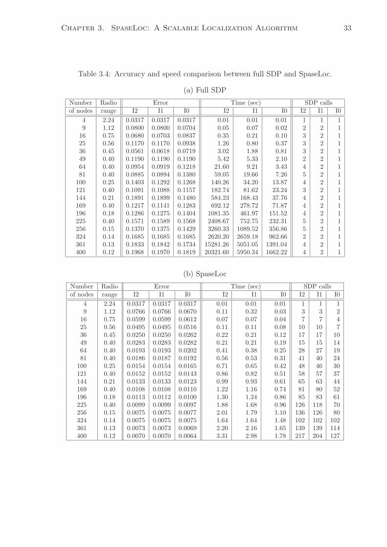
Chapter 3. SpaseLoc: A Scalable Localization Algorithm 33
Table 3.4: Accuracy and speed comparison between full SDP and SpaseLoc.
(a) Full SDP
Number Radio Error Time (sec) SDP callsof nodes range I2 I1 I0 I2 I1 I0 I2 I1 I0
4 2.24 0.0317 0.0317 0.0317 0.01 0.01 0.01 1 1 19 1.12 0.0800 0.0800 0.0704 0.05 0.07 0.02 2 2 1
16 0.75 0.0680 0.0703 0.0837 0.35 0.21 0.10 3 2 125 0.56 0.1170 0.1170 0.0938 1.26 0.80 0.37 3 2 136 0.45 0.0561 0.0618 0.0719 3.02 1.88 0.81 3 2 149 0.40 0.1190 0.1190 0.1190 5.42 5.33 2.10 2 2 164 0.40 0.0954 0.0919 0.1218 21.60 9.21 3.43 4 2 181 0.40 0.0885 0.0894 0.1380 59.05 19.66 7.26 5 2 1
100 0.25 0.1403 0.1292 0.1268 140.26 34.20 13.87 4 2 1121 0.40 0.1091 0.1088 0.1157 182.74 81.62 23.24 3 2 1144 0.21 0.1891 0.1899 0.1480 584.23 168.43 37.76 4 2 1169 0.40 0.1217 0.1141 0.1283 692.12 278.72 71.87 4 2 1196 0.18 0.1286 0.1275 0.1404 1081.35 461.97 151.52 4 2 1225 0.40 0.1571 0.1589 0.1568 2408.67 752.75 232.31 5 2 1256 0.15 0.1370 0.1375 0.1429 3260.33 1089.52 356.86 5 2 1324 0.14 0.1685 0.1685 0.1685 2620.20 2659.18 962.66 2 2 1361 0.13 0.1833 0.1842 0.1734 15281.26 5051.05 1391.04 4 2 1400 0.12 0.1968 0.1970 0.1819 20321.60 5950.34 1662.22 4 2 1
(b) SpaseLoc
Number Radio Error Time (sec) SDP callsof nodes range I2 I1 I0 I2 I1 I0 I2 I1 I0
4 2.24 0.0317 0.0317 0.0317 0.01 0.01 0.01 1 1 19 1.12 0.0766 0.0766 0.0670 0.11 0.32 0.03 3 3 2
16 0.75 0.0599 0.0599 0.0612 0.07 0.07 0.04 7 7 425 0.56 0.0495 0.0495 0.0516 0.11 0.11 0.08 10 10 736 0.45 0.0250 0.0250 0.0262 0.22 0.21 0.12 17 17 1049 0.40 0.0283 0.0283 0.0282 0.21 0.21 0.19 15 15 1464 0.40 0.0193 0.0193 0.0202 0.41 0.38 0.25 28 27 1981 0.40 0.0186 0.0187 0.0192 0.56 0.53 0.31 41 40 24
100 0.25 0.0154 0.0154 0.0165 0.71 0.65 0.42 48 46 30121 0.40 0.0152 0.0152 0.0143 0.86 0.82 0.51 58 57 37144 0.21 0.0133 0.0133 0.0123 0.99 0.93 0.61 65 63 44169 0.40 0.0108 0.0108 0.0110 1.22 1.16 0.74 81 80 52196 0.18 0.0113 0.0112 0.0100 1.30 1.24 0.86 85 83 61225 0.40 0.0099 0.0099 0.0097 1.88 1.68 0.96 126 118 70256 0.15 0.0075 0.0075 0.0077 2.01 1.79 1.10 136 126 80324 0.14 0.0075 0.0075 0.0075 1.64 1.64 1.48 102 102 102361 0.13 0.0073 0.0073 0.0069 2.20 2.16 1.65 139 139 114400 0.12 0.0070 0.0070 0.0064 3.31 2.98 1.78 217 204 127
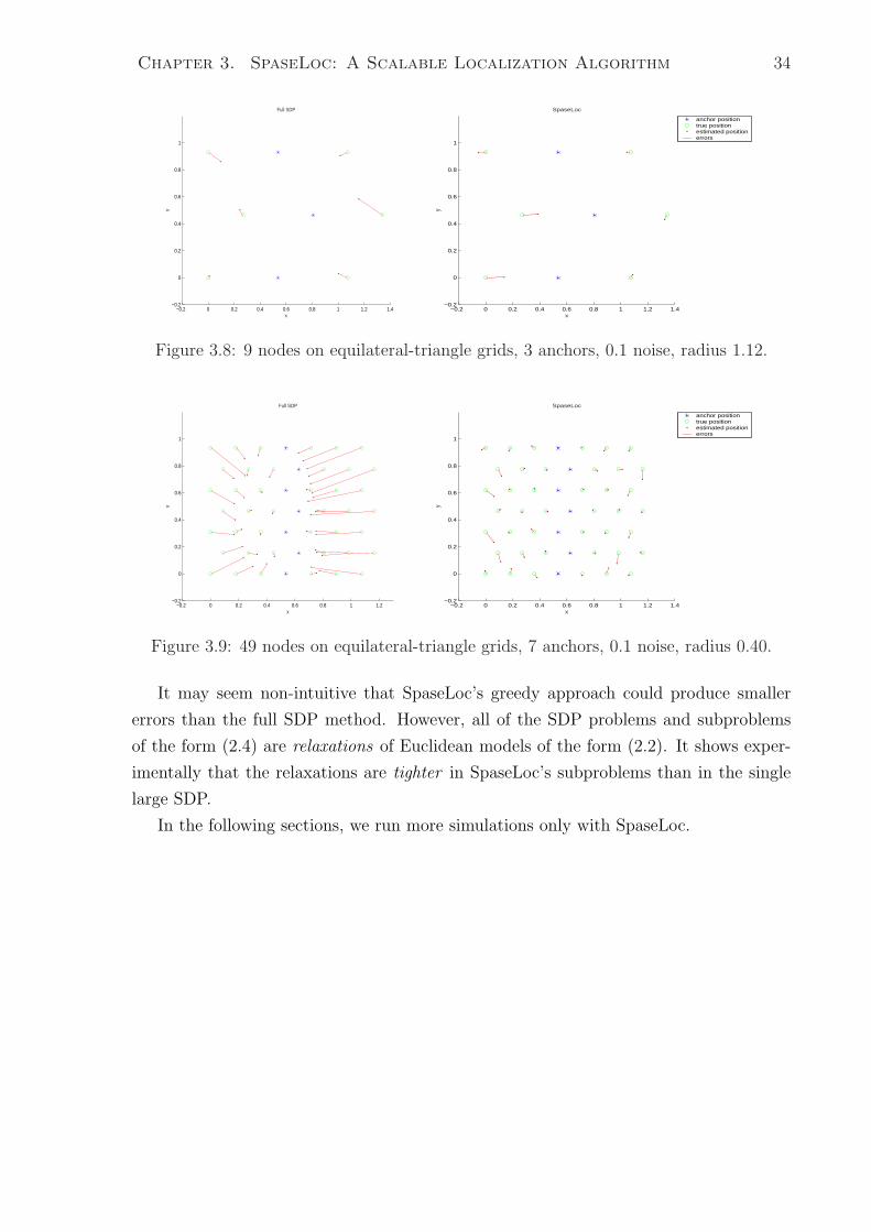
Chapter 3. SpaseLoc: A Scalable Localization Algorithm 34
−0.2 0 0.2 0.4 0.6 0.8 1 1.2 1.4−0.2
0
0.2
0.4
0.6
0.8
1
x
y
Full SDP
−0.2 0 0.2 0.4 0.6 0.8 1 1.2 1.4−0.2
0
0.2
0.4
0.6
0.8
1
x
y
SpaseLoc
anchor positiontrue positionestimated positionerrors
Figure 3.8: 9 nodes on equilateral-triangle grids, 3 anchors, 0.1 noise, radius 1.12.
−0.2 0 0.2 0.4 0.6 0.8 1 1.2−0.2
0
0.2
0.4
0.6
0.8
1
x
y
Full SDP
−0.2 0 0.2 0.4 0.6 0.8 1 1.2 1.4−0.2
0
0.2
0.4
0.6
0.8
1
x
y
SpaseLoc
anchor positiontrue positionestimated positionerrors
Figure 3.9: 49 nodes on equilateral-triangle grids, 7 anchors, 0.1 noise, radius 0.40.
It may seem non-intuitive that SpaseLoc’s greedy approach could produce smaller
errors than the full SDP method. However, all of the SDP problems and subproblems
of the form (2.4) are relaxations of Euclidean models of the form (2.2). It shows exper-
imentally that the relaxations are tighter in SpaseLoc’s subproblems than in the single
large SDP.
In the following sections, we run more simulations only with SpaseLoc.

Chapter 3. SpaseLoc: A Scalable Localization Algorithm 35
Table 3.5: SpaseLoc scalability. Strategies I2, I1, and I0 generate same results.
Nodes Anchors radius sub size Error 95% Error Trace 95% Trace Time SDP’s49 7 0.3412 2 1.40e-08 9.86e-10 6.28e-09 4.10e-10 0.21 21
100 10 0.2275 2 1.28e-07 8.78e-09 2.68e-08 2.36e-09 0.45 45225 15 0.1462 3 6.98e-07 7.74e-08 8.75e-08 1.19e-08 0.80 70529 23 0.0931 3 2.87e-06 9.42e-08 2.68e-07 1.03e-08 1.99 169
1089 33 0.0620 3 2.50e-06 1.65e-07 1.27e-07 1.12e-08 4.12 3502025 45 0.0451 3 2.70e-05 2.41e-07 2.28e-07 1.41e-08 8.55 6583969 63 0.0330 3 6.32e-06 3.53e-07 1.30e-07 1.39e-08 19.51 13025041 71 0.0292 3 6.70e-06 5.06e-07 1.44e-07 1.80e-08 25.57 16566084 78 0.0266 3 6.95e-06 5.47e-07 1.50e-07 1.84e-08 33.38 20007056 84 0.0247 4 5.92e-06 6.43e-07 1.35e-07 1.90e-08 41.58 17438100 90 0.0230 5 3.92e-06 6.42e-07 8.23e-08 1.78e-08 50.34 16029025 95 0.0218 5 8.38e-06 6.74e-07 1.17e-07 1.74e-08 57.34 1788
10000 100 0.0207 5 4.70e-06 7.63e-07 1.12e-07 1.94e-08 65.08 1981
3.3.3 Scalability
Table 3.5 shows simulation results for 49 to 10000 randomly uniform-distributed sensors
being localized using SpaseLoc with strategies I2, I1, and I0. The node numbers 49, 100,
225, . . . are squares k2, and the radius is the minimum value that permits localization
on a regular k × k grid. The number of anchors changes with the number of sensors in
order to maintain the same anchor density. Noise is not included in this simulation.
We find that the three strategies I2, I1, I0 produce the same results. This is because
the inaccuracy of the positioning estimation is purely caused by low connectivity, not by
noisy distance measurements. Empirically we see that the program scales well: almost
linearly in the number of nodes in the network. Indeed, the computational complexity of
the SpaseLoc algorithm is of order n, the number of sensors in the network, even though
the full SDP approach has much greater complexity, as we now show.
We know that in the full SDP model (2.4), the number of constraints is O(n2), and
in each of iteration of its interior-point algorithm the SDP solver needs to solve a sparse
linear system of equations whose dimension is the number of constraints. Figure 3.10
plots the CPU time for strategy I0 from Table 3.4 (a) as well as three curves of the form
time = apnp for p = 2, 3, 4, where ap is determined by a least-squares fit. It appears that
the SDP complexity with strategy I0 lies somewhere between O(n3) and O(n4).
In SpaseLoc, we partition the full problem into p subproblems of size q or less, where
p× q = n. We generally set q to be much smaller than n, ranging from 2 to around 10 in
most of our simulations. If τ represents the execution time taken by the full SDP method
for a 10-node network, in the worst case the computation time for SpaseLoc is τ ×O(p).
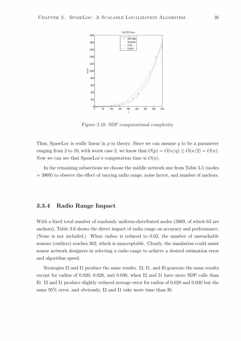
Chapter 3. SpaseLoc: A Scalable Localization Algorithm 36
0 50 100 150 200 250 300 350 4000
200
400
600
800
1000
1200
1400
1600
1800
2000
n
tim
e
Full SDP times
SDP dataQuadraticCubicQuartic
Figure 3.10: SDP computational complexity
Thus, SpaseLoc is really linear in p in theory. Since we can assume q to be a parameter
ranging from 2 to 10, with worst case 2, we know that O(p) = O(n/q) ≤ O(n/2) = O(n).
Now we can see that SpaseLoc’s computation time is O(n).
In the remaining subsections we choose the middle network size from Table 3.5 (nodes
= 3969) to observe the effect of varying radio range, noise factor, and number of anchors.
3.3.4 Radio Range Impact
With a fixed total number of randomly uniform-distributed nodes (3969, of which 63 are
anchors), Table 3.6 shows the direct impact of radio range on accuracy and performance.
(Noise is not included.) When radius is reduced to 0.02, the number of unreachable
sensors (outliers) reaches 302, which is unacceptable. Clearly, the simulation could assist
sensor network designers in selecting a radio range to achieve a desired estimation error
and algorithm speed.
Strategies I2 and I1 produce the same results. I2, I1, and I0 generate the same results
except for radius of 0.020, 0.028, and 0.030, when I2 and I1 have more SDP calls than
I0. I2 and I1 produce slightly reduced average error for radius of 0.028 and 0.030 but the
same 95% error, and obviously, I2 and I1 take more time than I0.
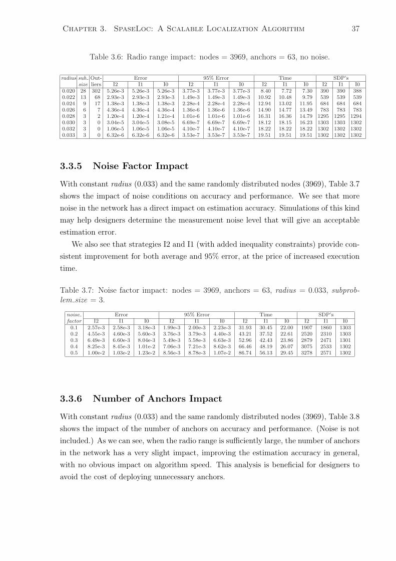
Chapter 3. SpaseLoc: A Scalable Localization Algorithm 37
Table 3.6: Radio range impact: nodes = 3969, anchors = 63, no noise.
radius sub Out- Error 95% Error Time SDP’ssize liers I2 I1 I0 I2 I1 I0 I2 I1 I0 I2 I1 I0
0.020 28 302 5.26e-3 5.26e-3 5.26e-3 3.77e-3 3.77e-3 3.77e-3 8.40 7.72 7.30 390 390 3880.022 13 68 2.93e-3 2.93e-3 2.93e-3 1.49e-3 1.49e-3 1.49e-3 10.92 10.48 9.79 539 539 5390.024 9 17 1.38e-3 1.38e-3 1.38e-3 2.28e-4 2.28e-4 2.28e-4 12.94 13.02 11.95 684 684 6840.026 6 7 4.36e-4 4.36e-4 4.36e-4 1.36e-6 1.36e-6 1.36e-6 14.90 14.77 13.49 783 783 7830.028 3 2 1.20e-4 1.20e-4 1.21e-4 1.01e-6 1.01e-6 1.01e-6 16.31 16.36 14.79 1295 1295 12940.030 3 0 3.04e-5 3.04e-5 3.08e-5 6.69e-7 6.69e-7 6.69e-7 18.12 18.15 16.23 1303 1303 13020.032 3 0 1.06e-5 1.06e-5 1.06e-5 4.10e-7 4.10e-7 4.10e-7 18.22 18.22 18.22 1302 1302 13020.033 3 0 6.32e-6 6.32e-6 6.32e-6 3.53e-7 3.53e-7 3.53e-7 19.51 19.51 19.51 1302 1302 1302
3.3.5 Noise Factor Impact
With constant radius (0.033) and the same randomly distributed nodes (3969), Table 3.7
shows the impact of noise conditions on accuracy and performance. We see that more
noise in the network has a direct impact on estimation accuracy. Simulations of this kind
may help designers determine the measurement noise level that will give an acceptable
estimation error.
We also see that strategies I2 and I1 (with added inequality constraints) provide con-
sistent improvement for both average and 95% error, at the price of increased execution
time.
Table 3.7: Noise factor impact: nodes = 3969, anchors = 63, radius = 0.033, subprob-lem size = 3.
noise Error 95% Error Time SDP’sfactor I2 I1 I0 I2 I1 I0 I2 I1 I0 I2 I1 I00.1 2.57e-3 2.58e-3 3.18e-3 1.99e-3 2.00e-3 2.23e-3 31.93 30.45 22.00 1907 1860 13030.2 4.55e-3 4.60e-3 5.60e-3 3.76e-3 3.79e-3 4.40e-3 43.21 37.52 22.61 2520 2310 13030.3 6.49e-3 6.60e-3 8.04e-3 5.49e-3 5.58e-3 6.63e-3 52.96 42.43 23.86 2879 2471 13010.4 8.25e-3 8.45e-3 1.01e-2 7.06e-3 7.21e-3 8.62e-3 66.46 48.19 26.07 3075 2533 13020.5 1.00e-2 1.03e-2 1.23e-2 8.56e-3 8.78e-3 1.07e-2 86.74 56.13 29.45 3278 2571 1302
3.3.6 Number of Anchors Impact
With constant radius (0.033) and the same randomly distributed nodes (3969), Table 3.8
shows the impact of the number of anchors on accuracy and performance. (Noise is not
included.) As we can see, when the radio range is sufficiently large, the number of anchors
in the network has a very slight impact, improving the estimation accuracy in general,
with no obvious impact on algorithm speed. This analysis is beneficial for designers to
avoid the cost of deploying unnecessary anchors.
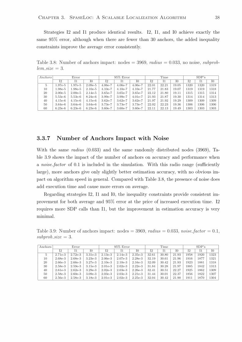
Chapter 3. SpaseLoc: A Scalable Localization Algorithm 38
Strategies I2 and I1 produce identical results. I2, I1, and I0 achieve exactly the
same 95% error, although when there are fewer than 30 anchors, the added inequality
constraints improve the average error consistently.
Table 3.8: Number of anchors impact: nodes = 3969, radius = 0.033, no noise, subprob-lem size = 3.
Anchors Error 95% Error Time SDP’sI2 I1 I0 I2 I1 I0 I2 I1 I0 I2 I1 I0
5 1.97e-5 1.97e-5 2.09e-5 4.06e-7 4.06e-7 4.06e-7 22.01 22.21 19.05 1320 1320 131910 1.98e-5 1.98e-5 2.10e-5 4.10e-7 4.10e-7 4.10e-7 21.77 21.83 19.07 1319 1319 131820 2.00e-5 2.00e-5 2.14e-5 3.65e-7 3.65e-7 3.65e-7 22.12 21.80 19.11 1315 1315 131430 5.53e-6 5.53e-6 8.24e-6 3.99e-7 3.99e-7 4.01e-7 21.93 21.87 19.30 1314 1314 131340 4.15e-6 4.15e-6 4.15e-6 3.62e-7 3.62e-7 3.62e-7 21.97 21.92 19.29 1309 1309 130950 3.64e-6 3.64e-6 3.64e-6 3.73e-7 3.73e-7 3.73e-7 22.02 22.23 19.36 1306 1306 130660 6.23e-6 6.23e-6 6.23e-6 3.60e-7 3.60e-7 3.60e-7 22.11 22.13 19.49 1303 1303 1303
3.3.7 Number of Anchors Impact with Noise
With the same radius (0.033) and the same randomly distributed nodes (3969), Ta-
ble 3.9 shows the impact of the number of anchors on accuracy and performance when
a noise factor of 0.1 is included in the simulation. With this radio range (sufficiently
large), more anchors give only slightly better estimation accuracy, with no obvious im-
pact on algorithm speed in general. Compared with Table 3.8, the presence of noise does
add execution time and cause more errors on average.
Regarding strategies I2, I1 and I0, the inequality constraints provide consistent im-
provement for both average and 95% error at the price of increased execution time. I2
requires more SDP calls than I1, but the improvement in estimation accuracy is very
minimal.
Table 3.9: Number of anchors impact: nodes = 3969, radius = 0.033, noise factor = 0.1,subprob size = 3.
Anchors Error 95% Error Time SDP’sI2 I1 I0 I2 I1 I0 I2 I1 I0 I2 I1 I0
5 2.71e-3 2.72e-3 3.31e-3 2.13e-3 2.14e-3 2.35e-3 32.61 30.80 21.93 1958 1920 132310 2.68e-3 2.68e-3 3.23e-3 2.06e-3 2.07e-3 2.28e-3 32.19 30.61 21.96 1916 1877 132120 2.66e-3 2.66e-3 3.27e-3 2.10e-3 2.10e-3 2.34e-3 32.09 30.42 21.93 1923 1881 131830 2.58e-3 2.59e-3 3.15e-3 2.01e-3 2.02e-3 2.22e-3 31.84 30.28 21.97 1885 1842 131340 2.61e-3 2.62e-3 3.29e-3 2.02e-3 2.03e-3 2.26e-3 32.41 30.51 22.27 1925 1862 130950 2.58e-3 2.60e-3 3.09e-3 2.03e-3 2.03e-3 2.21e-3 31.44 30.01 22.37 1856 1822 130760 2.56e-3 2.58e-3 3.18e-3 2.01e-3 2.02e-3 2.25e-3 32.04 30.42 21.90 1911 1870 1304
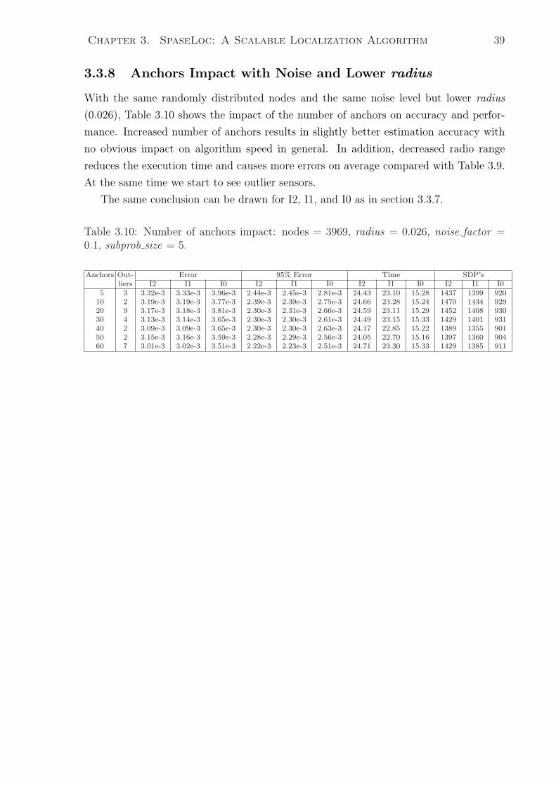
Chapter 3. SpaseLoc: A Scalable Localization Algorithm 39
3.3.8 Anchors Impact with Noise and Lower radius
With the same randomly distributed nodes and the same noise level but lower radius
(0.026), Table 3.10 shows the impact of the number of anchors on accuracy and perfor-
mance. Increased number of anchors results in slightly better estimation accuracy with
no obvious impact on algorithm speed in general. In addition, decreased radio range
reduces the execution time and causes more errors on average compared with Table 3.9.
At the same time we start to see outlier sensors.
The same conclusion can be drawn for I2, I1, and I0 as in section 3.3.7.
Table 3.10: Number of anchors impact: nodes = 3969, radius = 0.026, noise factor =0.1, subprob size = 5.
Anchors Out- Error 95% Error Time SDP’sliers I2 I1 I0 I2 I1 I0 I2 I1 I0 I2 I1 I0
5 3 3.32e-3 3.33e-3 3.96e-3 2.44e-3 2.45e-3 2.81e-3 24.43 23.10 15.28 1437 1399 92010 2 3.19e-3 3.19e-3 3.77e-3 2.39e-3 2.39e-3 2.75e-3 24.66 23.28 15.24 1470 1434 92920 9 3.17e-3 3.18e-3 3.81e-3 2.30e-3 2.31e-3 2.66e-3 24.59 23.11 15.29 1452 1408 93030 4 3.13e-3 3.14e-3 3.65e-3 2.30e-3 2.30e-3 2.61e-3 24.49 23.15 15.33 1429 1401 93140 2 3.09e-3 3.09e-3 3.65e-3 2.30e-3 2.30e-3 2.63e-3 24.17 22.85 15.22 1389 1355 90150 2 3.15e-3 3.16e-3 3.59e-3 2.28e-3 2.29e-3 2.56e-3 24.05 22.70 15.16 1397 1360 90460 7 3.01e-3 3.02e-3 3.51e-3 2.22e-3 2.23e-3 2.51e-3 24.71 23.30 15.33 1429 1385 911
Chapter 4
Moving Sensor Localizations
The previous chapter explains how static sensors are being localized using SpaseLoc. In
many applications, some of the sensors are dynamic. This chapter describes an algorithm
for moving sensor localization. We show that SpaseLoc can be applied to a series of static
localization problems to achieve the desired effect. Simulation results of this algorithm
are then presented. Our experiment shows that our proposed dynamic sensor localization
algorithm scales very well. For example, on a 2.4 GHz Pentium laptop the algorithm is
capable of localizing 500 moving sensors within a 4000-node network every one-second
time interval.
The last section discusses possible applications of the moving sensor localization algo-
rithm, with an illustrated example simulating a bus transit arrival-time reporting system.
4.1 Moving Sensor Localization Method
The main difference between a static localization network and a dynamic one is that the
distance measurements among sensors are constant in the first case, while some distance
measurements are changing in the second case because of the sensor movements. The
idea behind our moving sensor localization method is that at any given moment we can
take a static view of the dynamic sensor network. For each snapshot of the network with
all the sensors frozen in their positions and with the connection information among them,
we can utilize the static localization method SpaseLoc to estimate the locations of the
moving sensors at that particular instant. This provides an acceptable approximation if
the computation time is less than the interval between snapshots.
40
Chapter 4. Moving Sensor Localizations 41
4.1.1 Problem Formulation
We define tracking instant to be the instant of time that some sensors’ locations need to
be updated. There are two ways to trigger a tracking instant: either at a fixed frequency
after a given time interval, or upon detection of sensor movements, which are revealed
by changes in the distance measurement matrix d.
In order to track the moving sensors effectively, we need to isolate the sensors into
two categories. One is called static sensors, the other is called dynamic sensors. At any
given tracking instant, we assume that the static sensors are already localized by the
previous iteration and can be used as anchors by this iteration. There are two situations
in determining which sensors are dynamic. One situation is when the dynamic sensors
are specified ahead of time. We update all of their locations at all tracking instants,
regardless of whether they have moved or not since the previous instant. The other
situation is when any sensor could be static or dynamic at any instant. The ones that
have moved from the previous instant would be the dynamic ones. Under this situation,
we find which ones are moving by searching the distance matrix d for measurement
changes (refer to section 4.1.2 for a method to do this).
As mentioned, at any given instant t we can treat the dynamic sensor localization
problem as a static one and utilize SpaseLoc to localize the moving sensors at that
instant. Corresponding to the SpaseLoc problem definition in section 1.1, we formulate
the dynamic sensor localization problem as follows at tracking instant t.
Input
Total points : n, the total number of static and dynamic sensors, including anchors.
Unknown points : s sensors that are dynamic and whose locations xi ∈ R2, i = 1, . . . , s
are to be determined at tracking instant t.
Known points : m anchors that are static sensors and whose locations ak ∈ R2, k =
s + 1, . . . , n are known at tracking instant t.
Distance measurements : The distance matrix d consisting of dij and dik are the same
as explained in section 1.1, except d is partitioned according to
d =
(DIST11 m distance
m distance′ DIST22
), (4.1)
where DIST11 is an s by s matrix representing the distance measurements among
s dynamic sensors. In some applications, we do not use any distance measurements
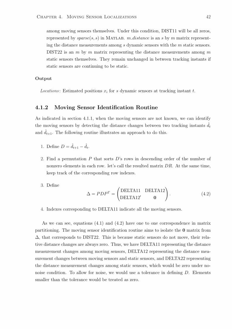
Chapter 4. Moving Sensor Localizations 42
among moving sensors themselves. Under this condition, DIST11 will be all zeros,
represented by sparse(s, s) in Matlab. m distance is an s by m matrix represent-
ing the distance measurements among s dynamic sensors with the m static sensors.
DIST22 is an m by m matrix representing the distance measurements among m
static sensors themselves. They remain unchanged in between tracking instants if
static sensors are continuing to be static.
Output
Locations : Estimated positions xi for s dynamic sensors at tracking instant t.
4.1.2 Moving Sensor Identification Routine
As indicated in section 4.1.1, when the moving sensors are not known, we can identify
the moving sensors by detecting the distance changes between two tracking instants dt
and dt+1. The following routine illustrates an approach to do this.
1. Define D = dt+1 − dt.
2. Find a permutation P that sorts D’s rows in descending order of the number of
nonzero elements in each row. let’s call the resulted matrix DR. At the same time,
keep track of the corresponding row indexes.
3. Define
∆ = PDP T =
(DELTA11 DELTA12
DELTA12′ 0
). (4.2)
4. Indexes corresponding to DELTA11 indicate all the moving sensors.
As we can see, equations (4.1) and (4.2) have one to one correspondence in matrix
partitioning. The moving sensor identification routine aims to isolate the 0 matrix from
∆, that corresponds to DIST22. This is because static sensors do not move, their rela-
tive distance changes are always zero. Thus, we have DELTA11 representing the distance
measurement changes among moving sensors, DELTA12 representing the distance mea-
surement changes between moving sensors and static sensors, and DELTA22 representing
the distance measurement changes among static sensors, which would be zero under no-
noise condition. To allow for noise, we would use a tolerance in defining D. Elements
smaller than the tolerance would be treated as zero.

Chapter 4. Moving Sensor Localizations 43
Figure 4.1 shows an example with 7 sensors at time t in (a) and at time t + 1 in (b).
Let’s assume distance measurements at t and t + 1 are
dt =
0 0 0 1 1.5 0 00 0 0 1 1.5 1 00 0 0 0 1.5 0 01 1 0 0 1 0 0
1.5 1.5 1.5 1 0 1 1.50 1 0 0 1 0 10 0 0 0 1.5 1 0
, dt+1 =
0 1 0 1 1.5 0 01 0 1 1.5 1 1.5 00 1 0 0 1.5 1 01 1.5 0 0 1 0 0
1.5 1 1.5 1 0 1 1.50 1.5 1 0 1 0 10 0 0 0 1.5 1 0
.
We illustrate that the moving sensor identification routine should point out that sensors
2 and 6 are the moving ones. After applying the first two steps, we have
D =
0 1 0 0 0 0 01 0 1 .5 −.5 .5 00 1 0 0 0 1 00 .5 0 0 0 0 00 −.5 0 0 0 0 00 .5 1 0 0 0 00 0 0 0 0 0 0
, PD =
1 0 1 .5 −.5 .5 00 .5 1 0 0 0 00 1 0 0 0 1 00 −.5 0 0 0 0 00 .5 0 0 0 0 00 1 0 0 0 0 00 0 0 0 0 0 0
.
After the third step, we have
∆ = PDP T =
0 .5 1 −.5 .5 1 0.5 0 1 0 0 0 01 1 0 0 0 0 0−.5 0 0 0 0 0 0.5 0 0 0 0 0 01 0 0 0 0 0 00 0 0 0 0 0 0
.
We know that DELTA11 corresponds to sensor indexes 2 and 6. From step 4, we know
that these two are the moving ones, which indeed are the ones that moved from time t
to time t + 1.
There is a situation when the number of moving sensors is greater than the number
of static sensors, and the moving sensors are all moving at the same direction at the
same speed. In this case, the above routine won’t apply. We illustrate this through an
example in Figure 4.2. Sensors 2 and 6 both move diagonally with the same distance.
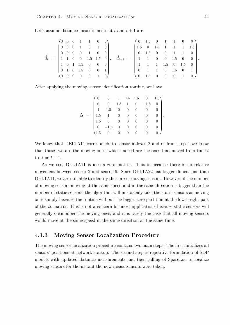
Chapter 4. Moving Sensor Localizations 44
Let’s assume distance measurements at t and t + 1 are
dt =
0 0 0 1 1 0 00 0 0 1 0 1 00 0 0 0 1 0 01 1 0 0 1.5 1.5 01 0 1 1.5 0 0 00 1 0 1.5 0 0 10 0 0 0 0 1 0
, dt+1 =
0 1.5 0 1 1 0 01.5 0 1.5 1 1 1 1.50 1.5 0 0 1 1 01 1 0 0 1.5 0 01 1 1 1.5 0 1.5 00 1 1 0 1.5 0 10 1.5 0 0 0 1 0
.
After applying the moving sensor identification routine, we have
∆ =
0 0 1 1.5 1.5 0 1.50 0 1.5 1 0 −1.5 01 1.5 0 0 0 0 0
1.5 1 0 0 0 0 01.5 0 0 0 0 0 00 −1.5 0 0 0 0 0
1.5 0 0 0 0 0 0
.
We know that DELTA11 corresponds to sensor indexes 2 and 6, from step 4 we know
that these two are the moving ones, which indeed are the ones that moved from time t
to time t + 1.
As we see, DELTA11 is also a zero matrix. This is because there is no relative
movement between sensor 2 and sensor 6. Since DELTA22 has bigger dimensions than
DELTA11, we are still able to identify the correct moving sensors. However, if the number
of moving sensors moving at the same speed and in the same direction is bigger than the
number of static sensors, the algorithm will mistakenly take the static sensors as moving
ones simply because the routine will put the bigger zero partition at the lower-right part
of the ∆ matrix. This is not a concern for most applications because static sensors will
generally outnumber the moving ones, and it is rarely the case that all moving sensors
would move at the same speed in the same direction at the same time.
4.1.3 Moving Sensor Localization Procedure
The moving sensor localization procedure contains two main steps. The first initializes all
sensors’ positions at network startup. The second step is repetitive formulation of SDP
models with updated distance measurements and then calling of SpaseLoc to localize
moving sensors for the instant the new measurements were taken.
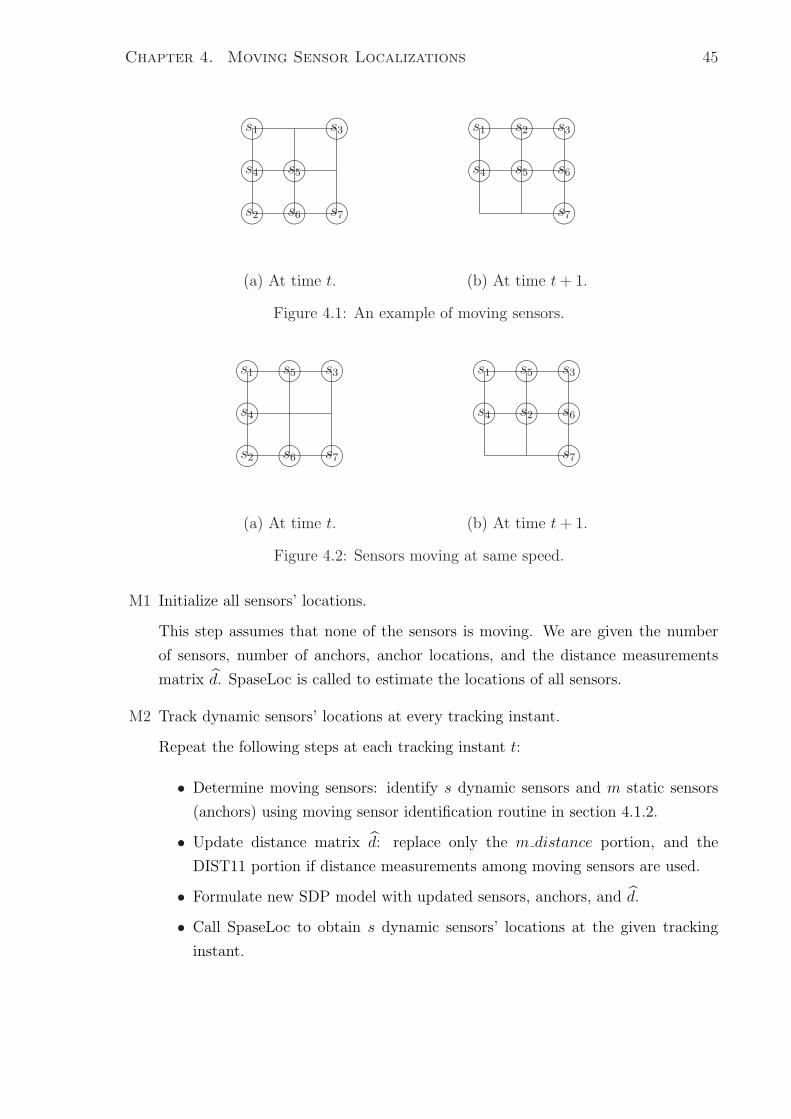
Chapter 4. Moving Sensor Localizations 45
±°²¯s1 ±°
²¯s3
±°²¯s4 ±°
²¯s5
±°²¯s2 ±°
²¯s6 ±°
²¯s7
±°²¯s1 ±°
²¯s2 ±°
²¯s3
±°²¯s4 ±°
²¯s5 ±°
²¯s6
±°²¯s7
(a) At time t. (b) At time t + 1.
Figure 4.1: An example of moving sensors.
±°²¯s1 ±°
²¯s5 ±°
²¯s3
±°²¯s4
±°²¯s2 ±°
²¯s6 ±°
²¯s7
±°²¯s1 ±°
²¯s5 ±°
²¯s3
±°²¯s4 ±°
²¯s2 ±°
²¯s6
±°²¯s7
(a) At time t. (b) At time t + 1.
Figure 4.2: Sensors moving at same speed.
M1 Initialize all sensors’ locations.
This step assumes that none of the sensors is moving. We are given the number
of sensors, number of anchors, anchor locations, and the distance measurements
matrix d. SpaseLoc is called to estimate the locations of all sensors.
M2 Track dynamic sensors’ locations at every tracking instant.
Repeat the following steps at each tracking instant t:
• Determine moving sensors: identify s dynamic sensors and m static sensors
(anchors) using moving sensor identification routine in section 4.1.2.
• Update distance matrix d: replace only the m distance portion, and the
DIST11 portion if distance measurements among moving sensors are used.
• Formulate new SDP model with updated sensors, anchors, and d.
• Call SpaseLoc to obtain s dynamic sensors’ locations at the given tracking
instant.
Chapter 4. Moving Sensor Localizations 46
In most moving sensor localization applications, seeking the best estimation accuracy
of the moving sensors’ locations might prove costly to real-time performance of the algo-
rithm. Our experiments in Chapter 3 show that SpaseLoc with the subsensor selection
priority rules introduced in section 3.1.3 generally achieves high estimation accuracy un-
der low connectivity and noise conditions. However, the moving sensor localization slows
down by about 20% for most of our test runs when we implement the priority rules listed
in Table 3.1. Hence, when there is sufficient connectivity among sensors in the network
and we trust that the network is not too noisy, it may be advantageous to simplify the
subsensor selection priority rules for greater real-time performance. We can achieve this
by reducing the total number of priorities for sensors and the number of acting levels for
acting anchors.
4.2 Moving Sensor Simulation Results
This section presents simulation results for the moving sensor localization algorithm.
The simulation setup is the same as in section 3.3 using strategy I0 except with added
information on dynamic sensors and distance updates at every tracking instant.
The simulation assumes a fixed number of moving sensors, and a given number of
time intervals of fixed length over which the dynamic sensors are to be tracked. The
movement pattern could be random or along some predefined path.
To simulate random movement of dynamic sensor i, we calculate the sensor’s position
at tracking instant t + 1 to be a random step from 0 to a maximum step of move size.
The following formula is used to generate sensor i’s next position from its current position
PP t(:, i):
PP t+1(:, i) = PP t(:, i) + move size ∗ (2 ∗ rand(2, 1)− 1).
Any points that fall outside the simulation area are regenerated.
As an example, Figure 4.3 shows the simulation results of one sensor moving di-
agonally through a 400-node randomly uniform-distributed sensor network. A red dot
represents the current position of the moving sensor, and the trail of yellow dots rep-
resents the trace of where the moving sensor has been. Following the moving sensor
localization procedure in the previous section, the network with 400 total nodes and 20
anchors is first localized by SpaseLoc. Initially, the moving sensor is intentionally posi-
tioned at the bottom left corner. Then at every time interval, the sensor moves with a
step of +0.1 in both x and y coordinates. The diagram shows the result of 10 movements.
We see that the algorithm localizes all 400 sensors initially with virtually no errors, and
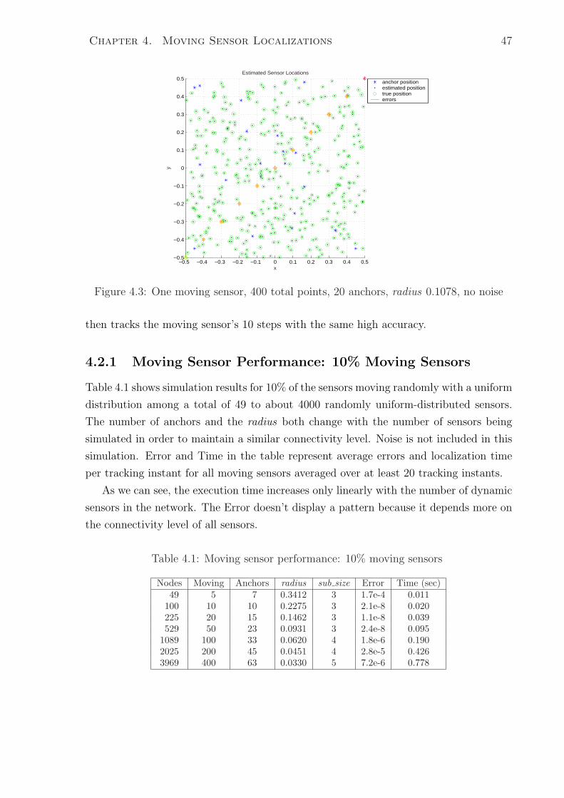
Chapter 4. Moving Sensor Localizations 47
−0.5 −0.4 −0.3 −0.2 −0.1 0 0.1 0.2 0.3 0.4 0.5−0.5
−0.4
−0.3
−0.2
−0.1
0
0.1
0.2
0.3
0.4
0.5
x
y
Estimated Sensor Locations
anchor positionestimated positiontrue positionerrors
Figure 4.3: One moving sensor, 400 total points, 20 anchors, radius 0.1078, no noise
then tracks the moving sensor’s 10 steps with the same high accuracy.
4.2.1 Moving Sensor Performance: 10% Moving Sensors
Table 4.1 shows simulation results for 10% of the sensors moving randomly with a uniform
distribution among a total of 49 to about 4000 randomly uniform-distributed sensors.
The number of anchors and the radius both change with the number of sensors being
simulated in order to maintain a similar connectivity level. Noise is not included in this
simulation. Error and Time in the table represent average errors and localization time
per tracking instant for all moving sensors averaged over at least 20 tracking instants.
As we can see, the execution time increases only linearly with the number of dynamic
sensors in the network. The Error doesn’t display a pattern because it depends more on
the connectivity level of all sensors.
Table 4.1: Moving sensor performance: 10% moving sensors
Nodes Moving Anchors radius sub size Error Time (sec)49 5 7 0.3412 3 1.7e-4 0.011
100 10 10 0.2275 3 2.1e-8 0.020225 20 15 0.1462 3 1.1e-8 0.039529 50 23 0.0931 3 2.4e-8 0.095
1089 100 33 0.0620 4 1.8e-6 0.1902025 200 45 0.0451 4 2.8e-5 0.4263969 400 63 0.0330 5 7.2e-6 0.778
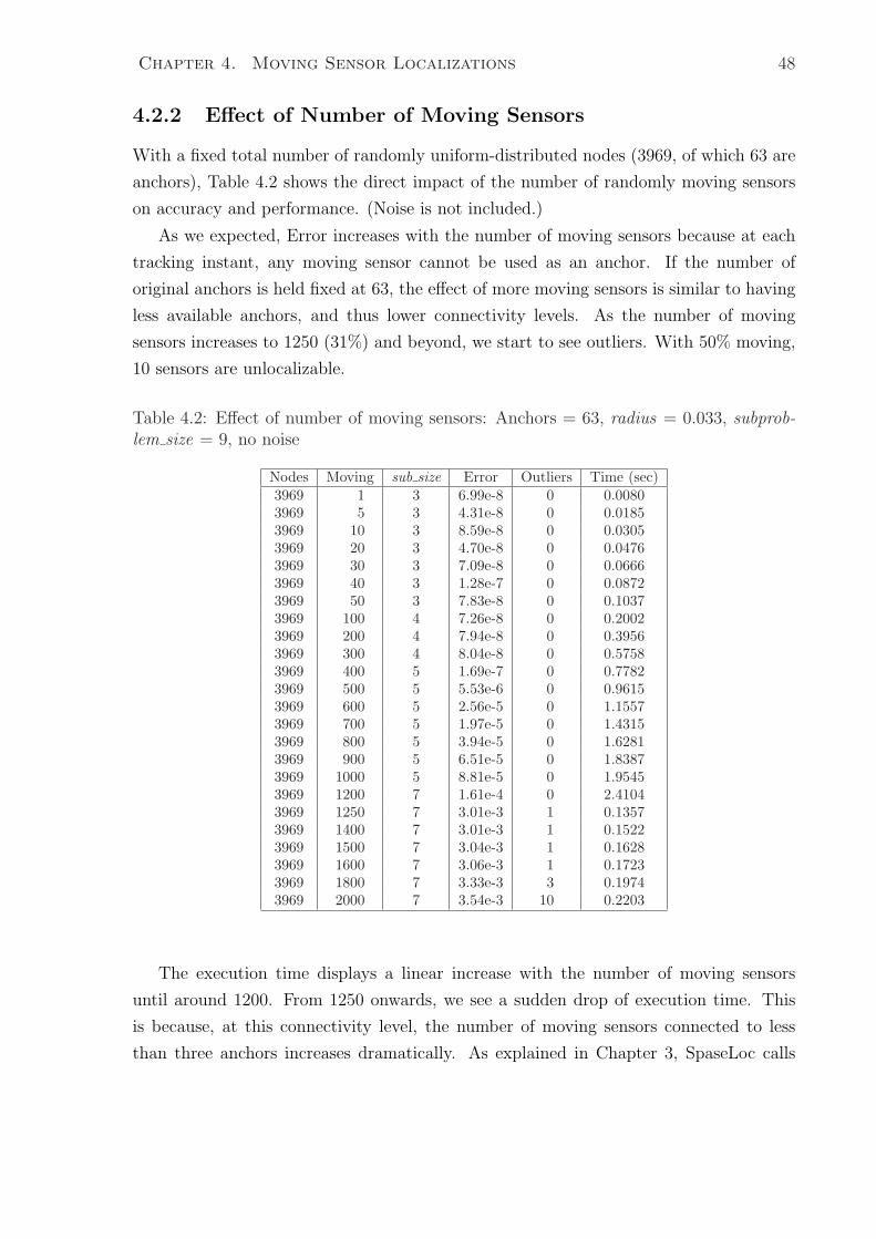
Chapter 4. Moving Sensor Localizations 48
4.2.2 Effect of Number of Moving Sensors
With a fixed total number of randomly uniform-distributed nodes (3969, of which 63 are
anchors), Table 4.2 shows the direct impact of the number of randomly moving sensors
on accuracy and performance. (Noise is not included.)
As we expected, Error increases with the number of moving sensors because at each
tracking instant, any moving sensor cannot be used as an anchor. If the number of
original anchors is held fixed at 63, the effect of more moving sensors is similar to having
less available anchors, and thus lower connectivity levels. As the number of moving
sensors increases to 1250 (31%) and beyond, we start to see outliers. With 50% moving,
10 sensors are unlocalizable.
Table 4.2: Effect of number of moving sensors: Anchors = 63, radius = 0.033, subprob-lem size = 9, no noise
Nodes Moving sub size Error Outliers Time (sec)3969 1 3 6.99e-8 0 0.00803969 5 3 4.31e-8 0 0.01853969 10 3 8.59e-8 0 0.03053969 20 3 4.70e-8 0 0.04763969 30 3 7.09e-8 0 0.06663969 40 3 1.28e-7 0 0.08723969 50 3 7.83e-8 0 0.10373969 100 4 7.26e-8 0 0.20023969 200 4 7.94e-8 0 0.39563969 300 4 8.04e-8 0 0.57583969 400 5 1.69e-7 0 0.77823969 500 5 5.53e-6 0 0.96153969 600 5 2.56e-5 0 1.15573969 700 5 1.97e-5 0 1.43153969 800 5 3.94e-5 0 1.62813969 900 5 6.51e-5 0 1.83873969 1000 5 8.81e-5 0 1.95453969 1200 7 1.61e-4 0 2.41043969 1250 7 3.01e-3 1 0.13573969 1400 7 3.01e-3 1 0.15223969 1500 7 3.04e-3 1 0.16283969 1600 7 3.06e-3 1 0.17233969 1800 7 3.33e-3 3 0.19743969 2000 7 3.54e-3 10 0.2203
The execution time displays a linear increase with the number of moving sensors
until around 1200. From 1250 onwards, we see a sudden drop of execution time. This
is because, at this connectivity level, the number of moving sensors connected to less
than three anchors increases dramatically. As explained in Chapter 3, SpaseLoc calls
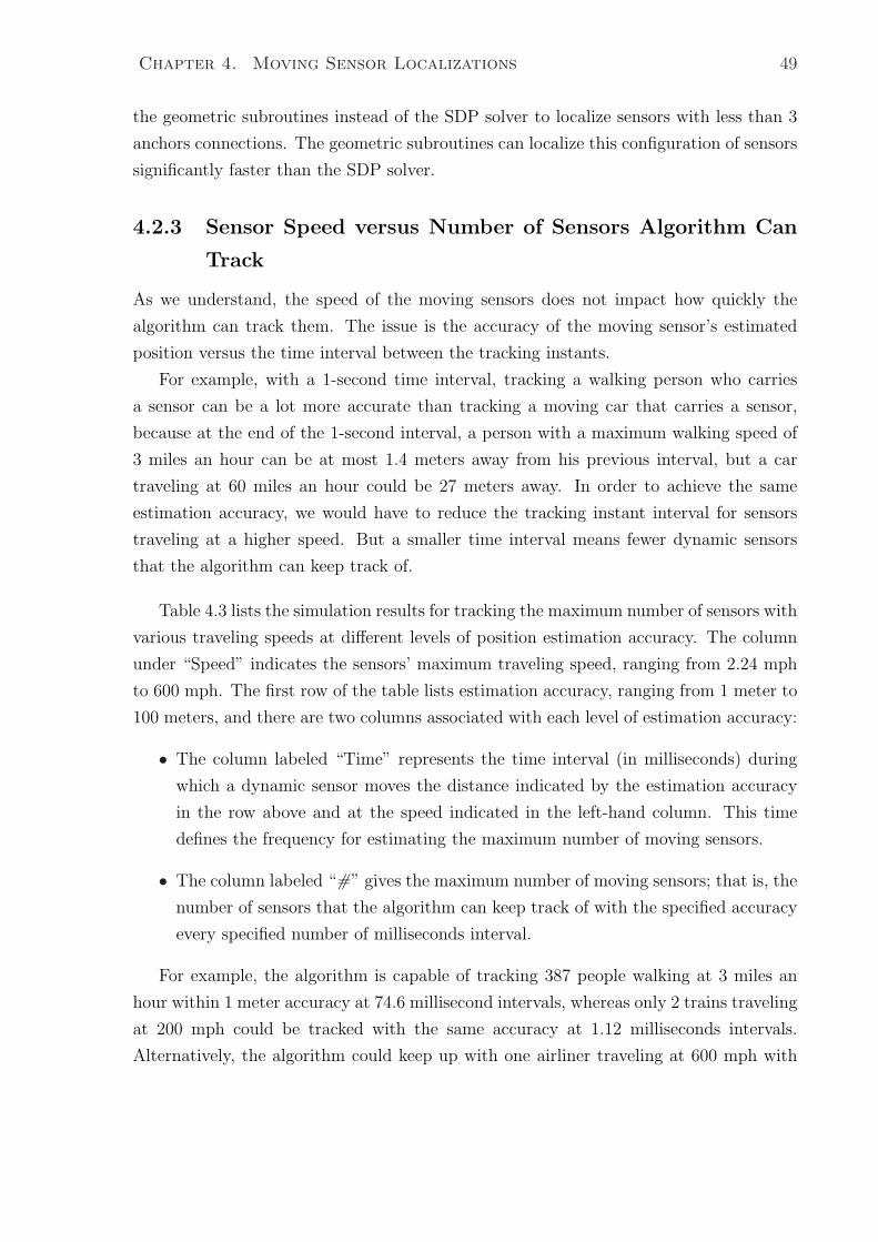
Chapter 4. Moving Sensor Localizations 49
the geometric subroutines instead of the SDP solver to localize sensors with less than 3
anchors connections. The geometric subroutines can localize this configuration of sensors
significantly faster than the SDP solver.
4.2.3 Sensor Speed versus Number of Sensors Algorithm Can
Track
As we understand, the speed of the moving sensors does not impact how quickly the
algorithm can track them. The issue is the accuracy of the moving sensor’s estimated
position versus the time interval between the tracking instants.
For example, with a 1-second time interval, tracking a walking person who carries
a sensor can be a lot more accurate than tracking a moving car that carries a sensor,
because at the end of the 1-second interval, a person with a maximum walking speed of
3 miles an hour can be at most 1.4 meters away from his previous interval, but a car
traveling at 60 miles an hour could be 27 meters away. In order to achieve the same
estimation accuracy, we would have to reduce the tracking instant interval for sensors
traveling at a higher speed. But a smaller time interval means fewer dynamic sensors
that the algorithm can keep track of.
Table 4.3 lists the simulation results for tracking the maximum number of sensors with
various traveling speeds at different levels of position estimation accuracy. The column
under “Speed” indicates the sensors’ maximum traveling speed, ranging from 2.24 mph
to 600 mph. The first row of the table lists estimation accuracy, ranging from 1 meter to
100 meters, and there are two columns associated with each level of estimation accuracy:
• The column labeled “Time” represents the time interval (in milliseconds) during
which a dynamic sensor moves the distance indicated by the estimation accuracy
in the row above and at the speed indicated in the left-hand column. This time
defines the frequency for estimating the maximum number of moving sensors.
• The column labeled “#” gives the maximum number of moving sensors; that is, the
number of sensors that the algorithm can keep track of with the specified accuracy
every specified number of milliseconds interval.
For example, the algorithm is capable of tracking 387 people walking at 3 miles an
hour within 1 meter accuracy at 74.6 millisecond intervals, whereas only 2 trains traveling
at 200 mph could be tracked with the same accuracy at 1.12 milliseconds intervals.
Alternatively, the algorithm could keep up with one airliner traveling at 600 mph with
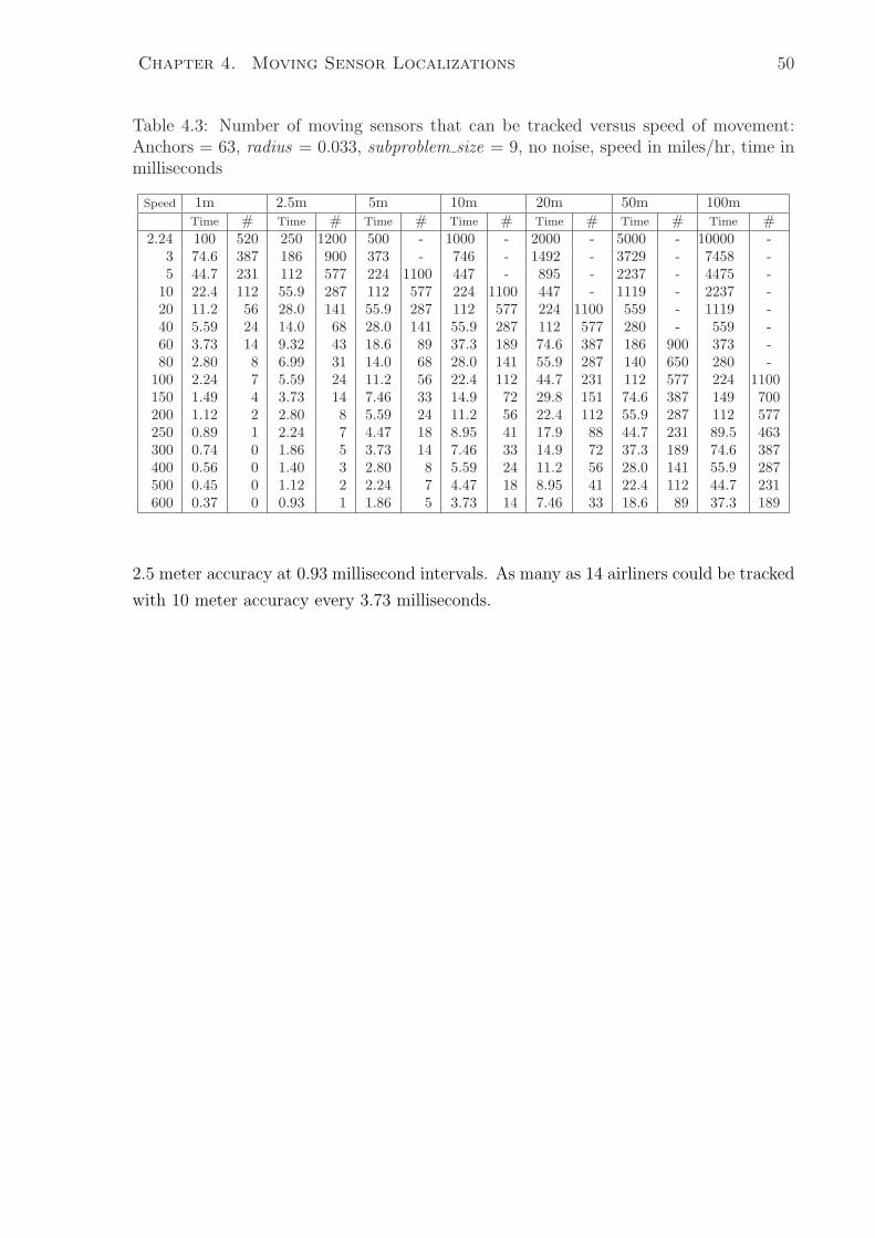
Chapter 4. Moving Sensor Localizations 50
Table 4.3: Number of moving sensors that can be tracked versus speed of movement:Anchors = 63, radius = 0.033, subproblem size = 9, no noise, speed in miles/hr, time inmilliseconds
Speed 1m 2.5m 5m 10m 20m 50m 100mTime # Time # Time # Time # Time # Time # Time #
2.24 100 520 250 1200 500 - 1000 - 2000 - 5000 - 10000 -3 74.6 387 186 900 373 - 746 - 1492 - 3729 - 7458 -5 44.7 231 112 577 224 1100 447 - 895 - 2237 - 4475 -
10 22.4 112 55.9 287 112 577 224 1100 447 - 1119 - 2237 -20 11.2 56 28.0 141 55.9 287 112 577 224 1100 559 - 1119 -40 5.59 24 14.0 68 28.0 141 55.9 287 112 577 280 - 559 -60 3.73 14 9.32 43 18.6 89 37.3 189 74.6 387 186 900 373 -80 2.80 8 6.99 31 14.0 68 28.0 141 55.9 287 140 650 280 -
100 2.24 7 5.59 24 11.2 56 22.4 112 44.7 231 112 577 224 1100150 1.49 4 3.73 14 7.46 33 14.9 72 29.8 151 74.6 387 149 700200 1.12 2 2.80 8 5.59 24 11.2 56 22.4 112 55.9 287 112 577250 0.89 1 2.24 7 4.47 18 8.95 41 17.9 88 44.7 231 89.5 463300 0.74 0 1.86 5 3.73 14 7.46 33 14.9 72 37.3 189 74.6 387400 0.56 0 1.40 3 2.80 8 5.59 24 11.2 56 28.0 141 55.9 287500 0.45 0 1.12 2 2.24 7 4.47 18 8.95 41 22.4 112 44.7 231600 0.37 0 0.93 1 1.86 5 3.73 14 7.46 33 18.6 89 37.3 189
2.5 meter accuracy at 0.93 millisecond intervals. As many as 14 airliners could be tracked
with 10 meter accuracy every 3.73 milliseconds.
Chapter 4. Moving Sensor Localizations 51
4.3 Applications of the Moving Sensor Localization
Algorithm
Dynamic sensor networks may find applications in many areas such as battlefield intel-
ligence, police patrol car tracking, taxi dispatching, car tracking in a car-share network,
road traffic monitoring, personnel monitoring, school bus tracking, and bus transit sched-
ule tracking. Most of these applications can be implemented using the global positioning
system (GPS) [9]. However, as we discussed in Chapter 1, several drawbacks of GPS
may prevent its successful use on a wide-range of real-time applications.
This section discusses how our dynamic sensor localization algorithm can be utilized
in such applications, with an implemented example simulating a bus transit scheduling
system. These applications all assume that the surrounding sensor network has sufficient
connectivity.
4.3.1 Battlefield Tracking System
An ad hoc wireless sensor network can be used to form a battlefield tracking system.
Static sensors can be spread around a battlefield by a helicopter. They may be used
to track enemy forces or friendly forces (depending on the type of sensor and who is
currently occupying the territory).
All soldiers could wear dynamic sensors in order to determine where their comrades
are in the adjacent neighborhood. At the same time, commanders could have a real-time
view of their troops’ positions by using our localization algorithm in order to assess the
current situation and direct the next move.
From Table 4.3, assuming soldiers run at a maximum speed of 5 miles an hour within
a 4000-node sensor network, we can see that our dynamic algorithm is capable of tracking
up to 231 soldiers within 1 meter accuracy in 44.7 millisecond intervals; up to 577 soldiers
within 2.5 meter accuracy every 112 milliseconds; and up to 1100 soldiers within 5 meter
accuracy every 224 milliseconds.
Another need in the battlefield is to track moving vehicles. In a hostile environment,
it can be difficult to communicate with the vehicle directly. We can set predefined moving
patterns or paths the vehicles are supposed to follow. Through the tracking traces of
the moving vehicles, the command center can analyze the environment each vehicle is in,
and how safe the vehicle is likely to be.
Chapter 4. Moving Sensor Localizations 52
4.3.2 Police Patrol Car Monitoring and Dispatching System
If we install enough static sensors to form an ad hoc wireless network for the patrol
environment, and if every police patrol car carries a sensor, the moving sensor localization
algorithm could find out where each patrol car is at each given instant. These locations
could be used to determine the nearest p police cars to a crime or accident scene, in order
to minimize the time for the p cars to arrive at the scene.
From Table 4.3, assuming that cars drive at a maximum of 100 mph within a 4000-
node sensor network, we see that our dynamic algorithm is capable of tracking up to 112
patrol cars with a 10 meter accuracy in 22.4 millisecond intervals, up to 231 cars with
a 20 meter accuracy every 44.7 milliseconds, up to 577 cars with a 50 meter accuracy
every 112 milliseconds, and so on.
Similar logic can be applied to taxi monitoring and dispatching. If we have all taxis
carry dynamic sensors, we can easily find the idle taxi nearest to the customer requiring
service.
4.3.3 Car Tracking in a Car-share Network
Car-sharing networks have been successfully deployed in Europe [14] and are becoming
popular in North America [30]. In a car network, a pool of cars are scattered around the
city to be shared by the network members. Ideally, a member should carry some type of
wireless device such as a PDA or a cell phone to locate and reserve the nearest idle car
anytime the person needs to rent it.
We can design an ad hoc wireless sensor network around the car-sharing network.
Each car in the network would carry a dynamic sensor, so at any time we would be able
to monitor the car’s location. At the same time, we also need to know the location of
the person needing the car rental in order to find the nearest available car. If we assume
the future ubiquitous presence of user-portable wireless data devices (like PDAs or cell
phones), we can envisage installing a dynamic sensor in the person’s hand-held wireless
device. For privacy reasons, the person could turn off the sensing device if he/she is
not using the car-sharing service. Our dynamic sensor localization algorithm could be
used in this system to track the locations of both cars and the people who are currently
looking for a shared car.
A similar method could be used for bike-sharing networks. Some cities like Copen-
hagen already offer bicycles for free use from a public pool. The service should become
more widely used if the matching of people to free bicycles can be implemented more
efficiently.
Chapter 4. Moving Sensor Localizations 53
4.3.4 Traffic Monitoring System
There have been many studies on the automated highway system, especially on the
development of an inter-vehicle communication system [28]. Such a system could be
used for dynamic traffic routing, driver assistance and navigation, co-operative driving
and platooning [41]. Singh [42] presents test results for an inter-vehicle communication
system based on a wireless LAN 802.11b network. The following proposes an alternative
approach to traffic monitoring.
Suppose static sensors are spread around major highways to form ad hoc wireless
sensor networks, and suppose cars carry dynamic sensors. We can evaluate highway
traffic conditions by tracking the movement of sensors within the cars. For example,
by looking at the current traces of most cars traveling on a particular highway, we can
determine the average actual speed of the cars. Comparing this speed with the maximum
speed of the highway, we can conclude if the highway is jammed or not. One by one,
we would be able to put all highways’ real-time traveling speed on a map maintained
by a central computing facility. The real-time speed map could be used by police patrol
officers, or by fire-fighters to predict a problem even before people could report a problem
on the road. At the same time, if a car’s display is connected to the central computing
facility, the car driver could download any portion of the map in real-time to decide on
the best option to his destination.
An even more proactive approach is to predefine the route a particular driver is to
take to his destination. If there are abnormal conditions on any road along the route,
the driver would be notified with a number of top alternative routes with estimated total
distance and travel times computed for him/her. An alternative is to mark the actual
speed on the map in real-time instants for the driver to reference while driving. We
could label different traffic conditions of highways according to the speed detected by the
sensors. For example, we could have 5 levels to represent traffic conditions, with level 1
being totally smooth and level 5 being totally blocked.
4.3.5 Personnel Monitoring System
Static sensors can be installed to form an ad hoc wireless sensor network in a limited
area such as a university campus, a corporate complex, a retail mall, or a prison camp
to monitor people’s movements for different purposes.
One example application is the prisoner monitoring system. Sensors could be worn
(or imbedded if permitted by law) by prisoners so that all their movements are actively
monitored. Legitimate movements and locations are ignored by the system, but if any
Chapter 4. Moving Sensor Localizations 54
prisoner appears to be too near the fence, for example, the system could alarm relevant
personnel immediately.
4.3.6 Bus Transit Arrival Reporting System
For most city’s public bus transit systems, there are fixed schedules for each bus route.
However, uncertainties on the road often cause the bus to be delayed, leaving new pas-
sengers waiting. In some cities with harsh climates, such as in Ottawa, Canada, there is a
phone number allocated for each bus stop. Passengers can phone for the arrival times of
the next coming bus and the one after that before heading to the bus stop, thus avoiding
a long wait in the cold during winter times. However, the times given to the callers are
mostly from a pre-recorded arrival schedule. If heavy traffic causes a certain bus to be
late, the caller would still be informed about the scheduled time, not the true delayed
time of arrival. It would be ideal if the schedule for each phone number and bus stop
were updated with more accurate arrival times based on the current locations of the next
two buses.
We propose a bus transit arrival reporting system utilizing our dynamic sensor lo-
calization algorithm. We assume each bus stop would be equipped with a static sensor,
and all buses would carry a dynamic sensor. If the distance between bus stops is bigger
than the sensor’s sensing range, we can add more static sensors in between to form an
ad hoc wireless sensor network. At each tracking instant, the algorithm would be able
to estimate each bus’s location in the network. We can calculate the estimated arrival
times of the two buses closest to a particular stop according to average traveling speed,
or if we have current road condition detection, we could use the current traveling speed
to estimate the expected arrival times of the two buses. This information is fed back to
the bus stop and passed on to the callers. We assume the future ubiquitous presence of
user-portable wireless data device (PDA or cell phone), or a fixed LED/LCD display at
each stop, to inform riders of the anticipated wait time for their current location.
Figure 4.4 shows a simulation run of a sample bus transit network. In this ad hoc
network, 400 green circles represent static sensors located at all bus stops and/or in
between bus stops, of which 39 are anchors with their locations known ahead of time.
These anchors are positioned in the middle of the network horizontally and vertically as
represented by the blue stars. Each adjacent two rows or columns of sensors represent a
vertical or horizontal street. Two buses are running on each street (represented by red
circles) with their initial positions at opposite ends of the street. (They are yellow in the
figure because yellow represents the traces of where a bus has been.)
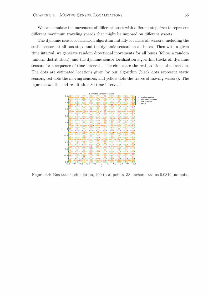
Chapter 4. Moving Sensor Localizations 55
We can simulate the movement of different buses with different step sizes to represent
different maximum traveling speeds that might be imposed on different streets.
The dynamic sensor localization algorithm initially localizes all sensors, including the
static sensors at all bus stops and the dynamic sensors on all buses. Then with a given
time interval, we generate random directional movements for all buses (follow a random
uniform distribution), and the dynamic sensor localization algorithm tracks all dynamic
sensors for a sequence of time intervals. The circles are the real positions of all sensors.
The dots are estimated locations given by our algorithm (black dots represent static
sensors, red dots the moving sensors, and yellow dots the traces of moving sensors). The
figure shows the end result after 30 time intervals.
−0.5 −0.4 −0.3 −0.2 −0.1 0 0.1 0.2 0.3 0.4 0.5−0.5
−0.4
−0.3
−0.2
−0.1
0
0.1
0.2
0.3
0.4
0.5
x
y
Estimated Sensor Locations
anchor positionestimated positiontrue positionerrors
Figure 4.4: Bus transit simulation, 400 total points, 38 anchors, radius 0.0819, no noise
Chapter 5
Distributed Algorithm For Clustered
Networks
As we have seen from previous discussions, existing localization methods have been prac-
tical for only moderate-sized networks (up to a few hundreds nodes), and SpaseLoc
maintains efficient and accurate position estimation for networks with up to ten thou-
sand sensors on a laptop computer with 2.4 GHz CPU and 1GB of system memory.
The variety and scale of future network applications begs for software that can fully
utilize the multitude of sensor devices currently being created. We would like to achieve
an enabling technology analogous to the device technology itself. Achieving the stated
objective for sensor localization—efficient and accurate localization for networks of arbi-
trary size—is an essential requirement for tomorrow’s wireless sensor networks to provide
their intended services. Thus, a further quantum leap is necessary to achieve true scal-
ability. The need is even more imperative when we recognize that the processing power
for the devices that may be used to run the localization algorithm in sensor networks of
the near future will be far less than the Pentium laptop that achieved our stated results.
Distributed computation becomes essential, as we propose in this chapter.
In this chapter, we first discuss the need for a distributed approach to sensor localiza-
tion and the intrinsic clustering architecture of large sensor networks; then we introduce
a hierarchical computational platform that can utilize distributed processing. Computa-
tional results for the proposed algorithm for a particular application are presented in the
last section.
56
Chapter 5. Distributed Algorithm For Clustered Networks 57
5.1 The Need for Distributed Computing
It is a scientific breakthrough that SpaseLoc is able to solve such large problems with
excellent speed and accuracy. Nevertheless, our experiments show that when the num-
ber of sensors reaches beyond 10000 on our particular laptop, the memory requirement
becomes excessive. The single-processor environment with virtual memory is not able to
proceed effectively for problems of that size.
Thus, in real network applications, SpaseLoc may face two challenges:
• The predicted explosive deployment of wireless sensor networks may involve tens of
thousands of sensors per network in the future. In such large networks, centralized
computing is simply not practical. Another quantum leap in algorithm performance
is urgently needed.
• In some applications, there is no device in the network as powerful as even a 2GHz
laptop computer to run the sensor localization algorithm (like SpaseLoc). We may
have to choose multiple smaller devices, which are used as sensors at the same
time, to compute the sensors’ locations collectively in the network. These devices
may be hand-held devices like PDAs, which currently have very limited processing
speed and system memory (probably only 30MHz and 256KB RAM). This forces
us to think about computing the sensors’ locations distributively among multiple
devices.
5.2 Clustered Sensor Network Architecture
Fortunately, large sensor networks are generally inherently clustered by design. One such
network proposed by Heinzelman et al. [18] exhibits the following characteristics:
• A hierarchical adaptive clustering architecture is recommended for scalability and
energy saving.
• Sensors are partitioned into clusters. Each cluster has a cluster head, and each
sensor belongs to one cluster.
• Dynamic cluster head selection is adopted. All cluster heads broadcast announce-
ments at system startup. When a sensor hears these announcements, it chooses
the cluster head from which the strongest signal is received. Essentially, a sensor
selects the nearest cluster head.
Chapter 5. Distributed Algorithm For Clustered Networks 58
• Application software, for example the localization algorithm, resides in the cluster
head.
• There is a multi-layer communication hierarchy. Sensors communicate only with
their own cluster heads. All cluster heads communicate with a central command
center. Depending on the particular implementation, cluster heads may be able to
communicate directly among themselves.
The proposed distributed sensor localization algorithm makes use of the clustering
architecture by adopting a hierarchical method in a distributed computing environment,
in order to address networks of any size and topology.
5.3 Distributed Sensor Localization Approach
Taking advantage of the intrinsic clustering of large networks, such as the one proposed in
section 5.2, we propose a hierarchical computational scheme that can utilize distributed
computing for sensor localization. SpaseLoc remains a vital yet intrinsically sequential
tool at a lower level. Scalability is achieved through parallelism at the cluster head level.
The proposed distributed algorithm utilizes three levels of machine devices as imposed
by the clustered sensor network architecture, and three levels of software (algorithm)
structure.
The top-level machine is regarded as a central command center and has relatively
more computing power, like a desktop PC. The second-level machines constitute the
cluster level; they are the cluster heads. These machines are generally devices that have
less computing power, like a current PDA. The lowest level devices are the sensors that
communicate with their own cluster heads. These devices generally don’t handle any
applications. They have signal communications with their neighboring sensors and with
their own cluster heads to report distance information, for instance.
The three levels of software structure are as follows:
distributed algorithm,
cluster-level algorithm,
subproblem algorithm.
The top-level algorithm is the distributed algorithm that we are proposing. It is respon-
sible for distributing a subset of anchors, sensors, and connection information to each
cluster head in order for each cluster head to know when and how to conduct sensor
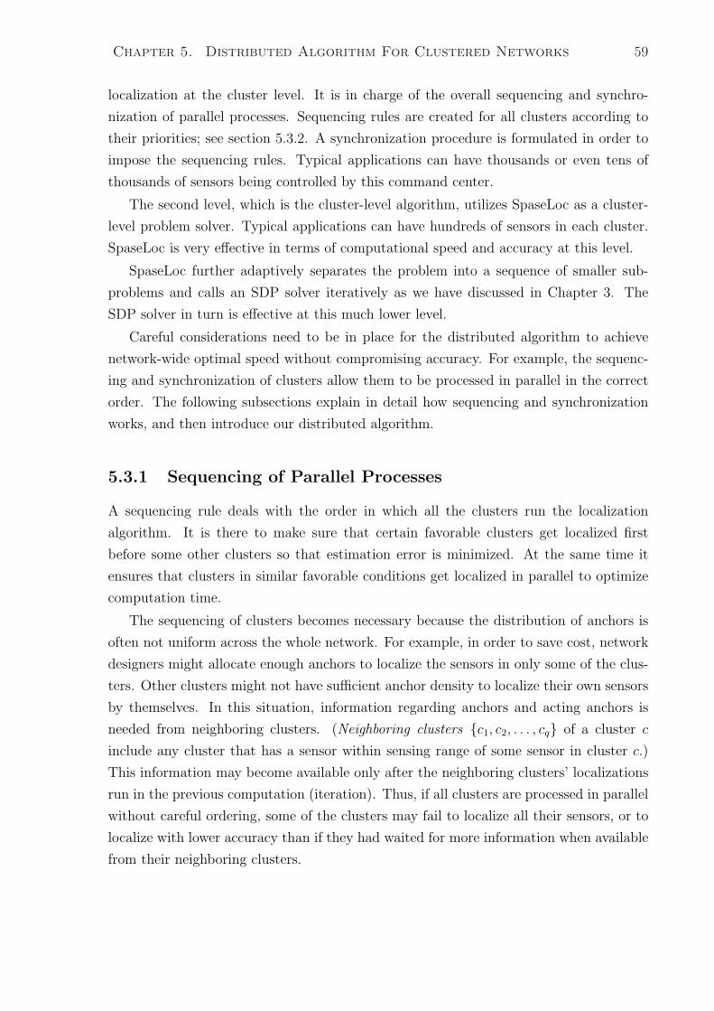
Chapter 5. Distributed Algorithm For Clustered Networks 59
localization at the cluster level. It is in charge of the overall sequencing and synchro-
nization of parallel processes. Sequencing rules are created for all clusters according to
their priorities; see section 5.3.2. A synchronization procedure is formulated in order to
impose the sequencing rules. Typical applications can have thousands or even tens of
thousands of sensors being controlled by this command center.
The second level, which is the cluster-level algorithm, utilizes SpaseLoc as a cluster-
level problem solver. Typical applications can have hundreds of sensors in each cluster.
SpaseLoc is very effective in terms of computational speed and accuracy at this level.
SpaseLoc further adaptively separates the problem into a sequence of smaller sub-
problems and calls an SDP solver iteratively as we have discussed in Chapter 3. The
SDP solver in turn is effective at this much lower level.
Careful considerations need to be in place for the distributed algorithm to achieve
network-wide optimal speed without compromising accuracy. For example, the sequenc-
ing and synchronization of clusters allow them to be processed in parallel in the correct
order. The following subsections explain in detail how sequencing and synchronization
works, and then introduce our distributed algorithm.
5.3.1 Sequencing of Parallel Processes
A sequencing rule deals with the order in which all the clusters run the localization
algorithm. It is there to make sure that certain favorable clusters get localized first
before some other clusters so that estimation error is minimized. At the same time it
ensures that clusters in similar favorable conditions get localized in parallel to optimize
computation time.
The sequencing of clusters becomes necessary because the distribution of anchors is
often not uniform across the whole network. For example, in order to save cost, network
designers might allocate enough anchors to localize the sensors in only some of the clus-
ters. Other clusters might not have sufficient anchor density to localize their own sensors
by themselves. In this situation, information regarding anchors and acting anchors is
needed from neighboring clusters. (Neighboring clusters {c1, c2, . . . , cq} of a cluster c
include any cluster that has a sensor within sensing range of some sensor in cluster c.)
This information may become available only after the neighboring clusters’ localizations
run in the previous computation (iteration). Thus, if all clusters are processed in parallel
without careful ordering, some of the clusters may fail to localize all their sensors, or to
localize with lower accuracy than if they had waited for more information when available
from their neighboring clusters.
Chapter 5. Distributed Algorithm For Clustered Networks 60
rc21
rc22
rc23
rc24
rc25
rc16
rc17
rc18
rr rc19
rc20
rc11
rc12
rc13
rc14
rc15
rc6
rc7
rr rc8
rc9
rr rc10
rc1
rc2
rc3
rc4
rc5
Figure 5.1: An example of a sensor network with 25 clusters.
For example, Figure 5.1 shows a sensor network of 25 squared clusters {c1, c2, . . . , c25}.The following are assumptions for the network:
• Each cluster head is an anchor and is located in the center of each square cluster;
denoted by a black dot (•) in the picture.
• Three clusters {c7, c9, c18} have two extra anchors (denoted by two extra black dots
(•) in the picture) that are within communication range of each other and their
cluster head.
• All other sensors in the network (not shown in the picture) are almost uniformly
distributed around the network. (Of course, we don’t know this before the local-
ization).
• The square borders for each cluster are assumed; they don’t necessarily have to
follow the exact square shape. We draw them that way for easy display.
Given the above conditions, we can clearly see that at the beginning of the localization,
only the three clusters {c7, c9, c18} with three original anchors should be localized first.
And since they are in similar anchor conditions, they can all be processed in parallel. All
the other clusters have only one anchor at this time (iteration); they would not achieve
good estimation accuracy if they were localized before {c7, c9, c18} are localized. We also
notice that clusters {c21, c25} should wait longer than the rest of the one-anchor clusters,
until after one of their neighboring clusters has been localized.
We propose a priority-driven cluster-labeling approach to address this sequencing
need, as presented in the next subsection.
Chapter 5. Distributed Algorithm For Clustered Networks 61
5.3.2 Cluster Priority
In our approach, all clusters are labeled with numerical values, called cluster priorities,
to indicate their sequencing order. Clusters with a smaller priority value have the higher
priority and are localized before clusters with a bigger priority value. Clusters with the
same priority can be localized in parallel at any time.
Many factors can be considered in classifying the clusters’ priorities. Here are some
important ones:
1. Original anchor density in the cluster.
For better accuracy, a cluster with higher anchor density within its own cluster
should be considered higher priority than the one with lower anchor density. In
Figure 5.1, cluster c18 with 3 original anchors is assigned higher priority than say
clusters c16, c17, c22, which have only one original anchor within each cluster.
2. The cluster’s neighbor-priority and the number of neighboring clusters with that
priority.
We define the a cluster’s neighbor-priority to be the the highest priority among all
the cluster’s neighboring clusters. Let’s assume a cluster c has neighboring clusters
{c1, c2, . . . , cq}, the highest priority among all q clusters is h, and the number of
clusters with this priority h is p. We say that cluster c’s neighbor-priority is h, and
there are p ≤ q neighboring clusters with that priority.
If cluster c has to rely on its neighboring clusters’ information to localize itself, a
higher neighbor-priority h will give cluster c a higher priority than that of a cluster
with a lower neighbor-priority h. For example in Figure 5.1, among all of cluster
c23’s neighboring clusters {c17, c18, c19, c22, c24}, c18 has the highest priority. So the
cluster priority associated with c18 determines the neighbor-priority for c23. We
know from the previous factor that cluster c18 has a higher priority than any of
c21’s neighboring clusters {c16, c17, c22}. So, cluster c23 will be assigned a higher
priority than cluster c21.
When two clusters have the same neighbor-priority h, the one with the bigger
number p will rank with higher priority. For example in Figure 5.1, clusters c19 and
c13 have the same neighbor-priority, both defined by cluster c18’s priority. However,
we know that cluster c13 has 3 neighboring clusters at this priority {c7, c9, c18 }, so
p = 3 for cluster c13, while p = 1 for cluster c19. Therefore, cluster c13 is assigned
higher priority than c19.
Chapter 5. Distributed Algorithm For Clustered Networks 62
3. The priority and number of anchors that are in the cluster’s neighboring clusters
and are within any of the cluster’s sensors’ radio range.
Let’s define a cluster’s neighboring anchors to be all the anchors in the cluster’s
neighboring clusters that have distance measurements with any sensor in this clus-
ter. A cluster associated with more neighboring anchors and with more neighboring
anchors at lower anchor levels will be assigned a higher priority than one with fewer
neighboring anchors and with more neighboring anchors at higher anchor levels.
Depending on the applications, designers may choose to consider all these factors in
determining the cluster priorities, or simply select any combination of them. Different
granularity of the cluster priorities can be achieved by specifying a range of the above
factors rather than specific values.
We give an example for a specific wireless sensor network application that utilizes the
first two criteria in assigning a cluster’s priority. A wireless sensor network may be used
to detect environmental hazards over a region by using individual sensors in the network
to detect smoke, chemicals or temperatures, etc. Sensors are generally spread roughly on
regular square grids across the protected area according to hazard detection regulations.
For example, the hazard detection rule may require that all detectors (sensors) must be
within a certain distance of another detector (sensor) to guarantee coverage.
We wouldn’t need localization if all sensors could be placed perfectly uniformly on the
regular square grids at installation. In practice, only certain required anchors are put at
known spots; the sensors are placed roughly within the regulated distance without exact
knowledge of their locations. This might be caused by the fact that certain sensors have
to be further apart or closer to each other because of installation barriers such as a wall.
Or, it might be more efficient or convenient to install sensors on certain landmarks, such
as on doors, windows, etc. At system startup, we would need to run the localization
algorithm to determine all the sensors’ locations.
Typically, this type of network is divided into clusters, each with a cluster head. The
cluster head also acts as an original anchor. For most applications, cluster heads are too
far apart from each other to be used as a group of 3 anchors to localize other sensors. For
localization to function, one or more of the clusters must add at least two extra anchors
that are within its cluster head’s and each other’s certain communication range (usually
within radio range of each other would be sufficient). The example shown in Figure 5.1
represents one such network.
Combining criteria 1 and 2 for assigning cluster priority, we give the following routine
designed to determine the cluster priority for such a network.
Chapter 5. Distributed Algorithm For Clustered Networks 63
Cluster Priority Assignment Routine:
1. Find all clusters that have 3 original anchors, and assign all these clusters priority
10 (the smallest priority value but the highest priority).
For example, in Figure 5.1, clusters {c7, c9, c18} all have three original anchors, so
they are all assigned cluster priority 10.
Table 5.1 tabulates partial cluster priority assignment rules for such a network.
As we can see from the first row, when the cluster is a 3-anchor cluster itself, the
cluster is assigned cluster priority 10.
2. If all clusters have been assigned a priority, go to Step 4. Otherwise go to Step 3.
3. For each cluster that has not been assigned a priority, find the cluster c that has the
highest neighbor-priority, h. To avoid too many cluster priorities being generated
in this step, we classify the neighbor-priorities that have the same first digit (say s)
as one category and count them all towards the number p. Thus, we set p to be the
number of neighboring clusters whose priorities have the same first digit as cluster
c’s neighbor-priority, h. Next, we assign cluster c’s priority to be (10(s+1)−p+9).
(We assume that a cluster has a maximum of 8 neighboring clusters.) For most
applications, the design of network would inherently limit the cluster priorities to
never go beyond the 100 range. The cluster priority calculation will therefore apply.
For example in Figure 5.1, cluster c13 has 3 neighboring clusters with priority 10.
This cluster will be assigned priority (10(1 + 1)− 3 + 9 = 26), as listed in the 7th
row in Table 5.1.
4. Report all cluster priorities and stop.
Going through the whole Cluster Priority Assignment routine for the example in
Figure 5.1, we obtain the cluster priorities listed in Table 5.2.
5.3.3 Synchronization among Parallel Processes
As we discussed in section 5.3.1, after the cluster priorities are assigned, a sequence
of clusters is generated from these priorities to determine the order of localization for
each cluster. A cluster with a higher priority goes before a cluster with a lower priority.
Clusters with the same priority go in parallel.
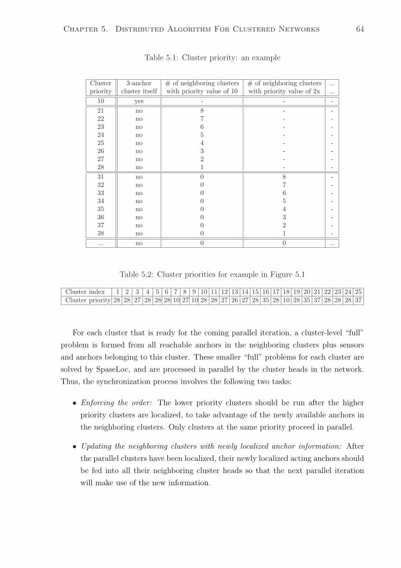
Chapter 5. Distributed Algorithm For Clustered Networks 64
Table 5.1: Cluster priority: an example
Cluster 3-anchor # of neighboring clusters # of neighboring clusters ...priority cluster itself with priority value of 10 with priority value of 2x ...
10 yes - - -21 no 8 - -22 no 7 - -23 no 6 - -24 no 5 - -25 no 4 - -26 no 3 - -27 no 2 - -28 no 1 - -31 no 0 8 -32 no 0 7 -33 no 0 6 -34 no 0 5 -35 no 0 4 -36 no 0 3 -37 no 0 2 -38 no 0 1 -... no 0 0 ...
Table 5.2: Cluster priorities for example in Figure 5.1
Cluster index 1 2 3 4 5 6 7 8 9 10 11 12 13 14 15 16 17 18 19 20 21 22 23 24 25Cluster priority 28 28 27 28 28 28 10 27 10 28 28 27 26 27 28 35 28 10 28 35 37 28 28 28 37
For each cluster that is ready for the coming parallel iteration, a cluster-level “full”
problem is formed from all reachable anchors in the neighboring clusters plus sensors
and anchors belonging to this cluster. These smaller “full” problems for each cluster are
solved by SpaseLoc, and are processed in parallel by the cluster heads in the network.
Thus, the synchronization process involves the following two tasks:
• Enforcing the order: The lower priority clusters should be run after the higher
priority clusters are localized, to take advantage of the newly available anchors in
the neighboring clusters. Only clusters at the same priority proceed in parallel.
• Updating the neighboring clusters with newly localized anchor information: After
the parallel clusters have been localized, their newly localized acting anchors should
be fed into all their neighboring cluster heads so that the next parallel iteration
will make use of the new information.
Chapter 5. Distributed Algorithm For Clustered Networks 65
5.3.4 Distributed Sensor Localization Algorithm
After we explain how the sequencing and synchronization work under the distributed
approach, this section presents our distributed sensor localization algorithm that glues
these two processes together.
Distributed sensor localization algorithm:
1. Determine the cluster priority for each cluster in the network. This is done at the
command center machine level by the routine given in section 5.3.2.
2. At the command center machine, sequence the cluster localization order according
to cluster priorities. A cluster with a higher priority ranks before a cluster with
lower priority. Clusters with the same cluster priority are put in the same rank.
Hence, a list of cluster ranks is produced. Let’s assume that r ranks are produced.
For each rank i in the list, there is a list of cluster indexes l associated with i.
The list l could include one index, or multiple indexes, which means that there are
multiple clusters put in the same rank.
3. In the command center level: synchronize all cluster heads to do localizations.
• For each rank i from 1 to r:
• For all clusters in l of same rank i:
Request all cluster heads in l to localize their own sensors simultaneously. For
each cluster c in l, the cluster head does the following tasks in parallel:
– Formulate cluster-level “full” problem, consisting of all the sensors, an-
chors, and distance measurements among them in cluster c, and all the
anchor information from cluster c’s neighboring clusters that are within
cluster c’s radio range.
– Call SpaseLoc to solve the cluster-level “full” problem.
– Update all cluster c’s neighboring clusters with the newly localized acting
anchors.
– Report to the command center that localization is done.
• When the command center receives reports from all clusters in l that they’ve
finished localizing their own clusters, go to next i.
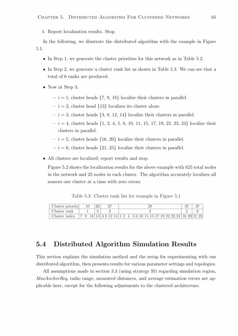
Chapter 5. Distributed Algorithm For Clustered Networks 66
4. Report localization results. Stop.
In the following, we illustrate the distributed algorithm with the example in Figure
5.1.
• In Step 1, we generate the cluster priorities for this network as in Table 5.2.
• In Step 2, we generate a cluster rank list as shown in Table 5.3. We can see that a
total of 6 ranks are produced.
• Now at Step 3,
– i = 1, cluster heads {7, 9, 18} localize their clusters in parallel.
– i = 2, cluster head {13} localizes its cluster alone.
– i = 3, cluster heads {3, 8, 12, 14} localize their clusters in parallel.
– i = 4, cluster heads {1, 2, 4, 5, 6, 10, 11, 15, 17, 19, 22, 23, 24} localize their
clusters in parallel.
– i = 5, cluster heads {16, 20} localize their clusters in parallel.
– i = 6, cluster heads {21, 25} localize their clusters in parallel.
• All clusters are localized; report results and stop.
Figure 5.2 shows the localization results for the above example with 625 total nodes
in the network and 25 nodes in each cluster. The algorithm accurately localizes all
sensors one cluster at a time with zero errors.
Table 5.3: Cluster rank list for example in Figure 5.1
Cluster priority 10 26 27 28 35 37Cluster rank 1 2 3 4 5 6Cluster index 7 9 18 13 3 8 12 14 1 2 4 5 6 10 11 15 17 19 22 23 24 16 20 21 25
5.4 Distributed Algorithm Simulation Results
This section explains the simulation method and the setup for experimenting with our
distributed algorithm, then presents results for various parameter settings and topologies.
All assumptions made in section 3.3 (using strategy I0) regarding simulation region,
MaxAnchorReq, radio range, measured distances, and average estimation errors are ap-
plicable here, except for the following adjustments to the clustered architecture.
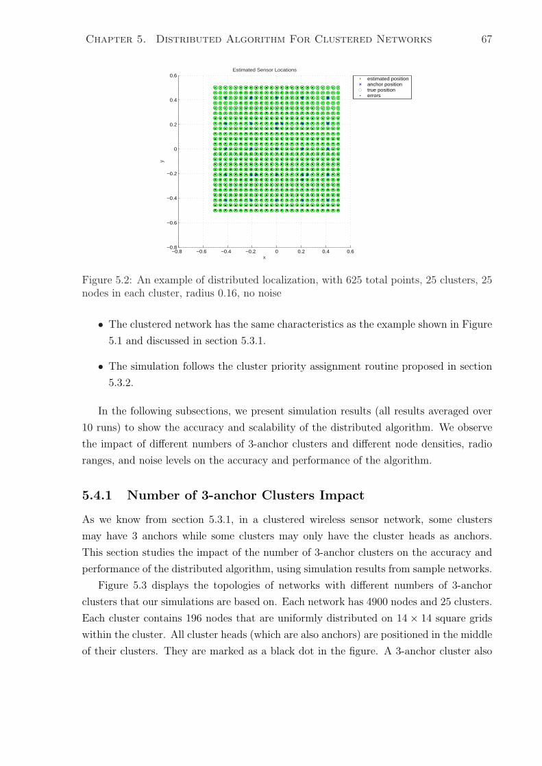
Chapter 5. Distributed Algorithm For Clustered Networks 67
−0.8 −0.6 −0.4 −0.2 0 0.2 0.4 0.6−0.8
−0.6
−0.4
−0.2
0
0.2
0.4
0.6
x
y
Estimated Sensor Locations
estimated positionanchor positiontrue positionerrors
Figure 5.2: An example of distributed localization, with 625 total points, 25 clusters, 25nodes in each cluster, radius 0.16, no noise
• The clustered network has the same characteristics as the example shown in Figure
5.1 and discussed in section 5.3.1.
• The simulation follows the cluster priority assignment routine proposed in section
5.3.2.
In the following subsections, we present simulation results (all results averaged over
10 runs) to show the accuracy and scalability of the distributed algorithm. We observe
the impact of different numbers of 3-anchor clusters and different node densities, radio
ranges, and noise levels on the accuracy and performance of the algorithm.
5.4.1 Number of 3-anchor Clusters Impact
As we know from section 5.3.1, in a clustered wireless sensor network, some clusters
may have 3 anchors while some clusters may only have the cluster heads as anchors.
This section studies the impact of the number of 3-anchor clusters on the accuracy and
performance of the distributed algorithm, using simulation results from sample networks.
Figure 5.3 displays the topologies of networks with different numbers of 3-anchor
clusters that our simulations are based on. Each network has 4900 nodes and 25 clusters.
Each cluster contains 196 nodes that are uniformly distributed on 14 × 14 square grids
within the cluster. All cluster heads (which are also anchors) are positioned in the middle
of their clusters. They are marked as a black dot in the figure. A 3-anchor cluster also
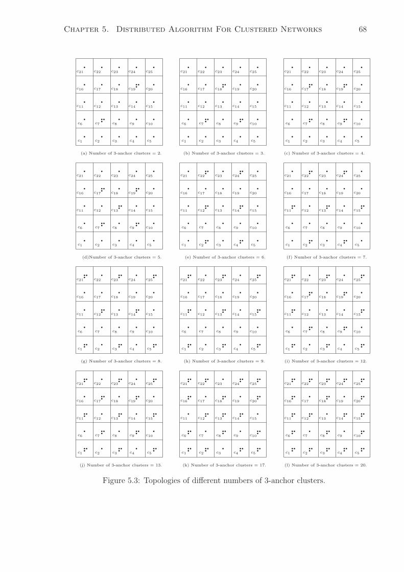
Chapter 5. Distributed Algorithm For Clustered Networks 68
qc21
qc22
qc23
qc24
qc25
qc16
qc17
qc18
qc19
qq qc20
qc11
qc12
qc13
qc14
qc15
qc6
qc7
qq qc8
qc9
qc10
qc1
qc2
qc3
qc4
qc5
qc21
qc22
qc23
qc24
qc25
qc16
qc17
qc18
qq qc19
qc20
qc11
qc12
qc13
qc14
qc15
qc6
qc7
qq qc8
qc9
qq qc10
qc1
qc2
qc3
qc4
qc5
qc21
qc22
qc23
qc24
qc25
qc16
qc17
qq qc18
qc19
qq qc20
qc11
qc12
qc13
qc14
qc15
qc6
qc7
qq qc8
qc9
qq qc10
qc1
qc2
qc3
qc4
qc5
(a) Number of 3-anchor clusters = 2. (b) Number of 3-anchor clusters = 3. (c) Number of 3-anchor clusters = 4.
qc21
qc22
qc23
qc24
qc25
qc16
qc17
qq qc18
qc19
qq qc20
qc11
qc12
qc13
qq qc14
qc15
qc6
qc7
qq qc8
qc9
qq qc10
qc1
qc2
qc3
qc4
qc5
qc21
qc22
qq qc23
qc24
qq qc25
qc16
qc17
qc18
qc19
qc20
qc11
qc12
qq qc13
qc14
qq qc15
qc6
qc7
qc8
qc9
qc10
qc1
qc2
qq qc3
qc4
qq qc5
qc21
qc22
qq qc23
qc24
qq qc25
qc16
qc17
qc18
qc19
qc20
qc11
qq qc12
qc13
qq qc14
qc15
qc6
qc7
qc8
qc9
qc10
qc1
qc2
qq qc3
qc4
qq qc5
(d)Number of 3-anchor clusters = 5. (e) Number of 3-anchor clusters = 6. (f) Number of 3-anchor clusters = 7.
qc21
qq qc22
qc23
qq qc24
qc25
qc16
qc17
qc18
qc19
qc20
qc11
qc12
qq qc13
qc14
qq qc15
qc6
qc7
qc8
qc9
qc10
qc1
qq qc2
qc3
qq qc4
qc5
qc21
qq qc22
qc23
qq qc24
qc25
qc16
qc17
qc18
qc19
qc20
qc11
qq qc12
qc13
qq qc14
qc15
qc6
qc7
qc8
qc9
qc10
qc1
qq qc2
qc3
qq qc4
qc5
qc21
qq qc22
qc23
qq qc24
qc25
qc16
qc17
qq qc18
qc19
qq qc20
qc11
qq qc12
qc13
qc14
qc15
qc6
qc7
qq qc8
qc9
qq qc10
qc1
qq qc2
qc3
qq qc4
qc5
(g) Number of 3-anchor clusters = 8. (h) Number of 3-anchor clusters = 9. (i) Number of 3-anchor clusters = 12.
qc21
qq qc22
qc23
qq qc24
qc25
qc16
qc17
qq qc18
qc19
qq qc20
qc11
qq qc12
qc13
qq qc14
qc15
qc6
qc7
qq qc8
qc9
qq qc10
qc1
qq qc2
qc3
qq qc4
qc5
qc21
qq qc22
qq qc23
qc24
qq qc25
qc16
qq qc17
qc18
qq qc19
qc20
qc11
qc12
qq qc13
qq qc14
qq qc15
qc6
qq qc7
qc8
qq qc9
qc10
qc1
qq qc2
qq qc3
qc4
qq qc5
qc21
qq qc22
qq qc23
qq qc24
qq qc25
qc16
qq qc17
qc18
qq qc19
qc20
qc11
qq qc12
qq qc13
qc14
qq qc15
qc6
qq qc7
qc8
qq qc9
qc10
qc1
qq qc2
qq qc3
qq qc4
qq qc5
(j) Number of 3-anchor clusters = 13. (k) Number of 3-anchor clusters = 17. (l) Number of 3-anchor clusters = 20.
Figure 5.3: Topologies of different numbers of 3-anchor clusters.
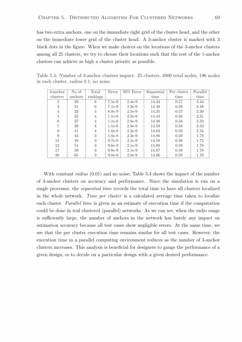
Chapter 5. Distributed Algorithm For Clustered Networks 69
has two extra anchors, one on the immediate right grid of the cluster head, and the other
on the immediate lower grid of the cluster head. A 3-anchor cluster is marked with 3
black dots in the figure. When we make choices on the locations of the 3-anchor clusters
among all 25 clusters, we try to choose their locations such that the rest of the 1-anchor
clusters can achieve as high a cluster priority as possible.
Table 5.4: Number of 3-anchor clusters impact: 25 clusters, 4900 total nodes, 196 nodesin each cluster, radius 0.1, no noise
3-anchor No of Total Error 95% Error Sequential Per cluster Parallelclusters anchors rankings time time time
2 29 6 7.5e-9 2.4e-9 14.34 0.57 3.443 31 6 7.1e-9 2.3e-9 14.48 0.58 3.484 33 4 8.0e-9 2.5e-9 14.35 0.57 2.305 35 4 1.1e-8 2.5e-9 14.43 0.58 2.316 37 4 1.1e-8 2.8e-9 14.48 0.58 2.327 39 4 1.1e-8 2.9e-9 14.59 0.58 2.338 41 4 1.0e-8 2.2e-9 14.63 0.59 2.349 43 3 1.0e-8 2.3e-9 14.86 0.59 1.78
12 49 3 9.7e-9 2.1e-9 14.58 0.58 1.7513 51 3 9.6e-9 2.1e-9 14.80 0.59 1.7817 59 3 9.8e-9 2.1e-9 14.87 0.59 1.7820 65 3 9.0e-9 2.0e-9 14.66 0.59 1.76
With constant radius (0.01) and no noise, Table 5.4 shows the impact of the number
of 3-anchor clusters on accuracy and performance. Since the simulation is run on a
single processor, the sequential time records the total time to have all clusters localized
in the whole network. Time per cluster is a calculated average time taken to localize
each cluster. Parallel time is given as an estimate of execution time if the computation
could be done in real clustered (parallel) networks. As we can see, when the radio range
is sufficiently large, the number of anchors in the network has barely any impact on
estimation accuracy because all test cases show negligible errors. At the same time, we
see that the per cluster execution time remains similar for all test cases. However, the
execution time in a parallel computing environment reduces as the number of 3-anchor
clusters increases. This analysis is beneficial for designers to gauge the performance of a
given design, or to decide on a particular design with a given desired performance.
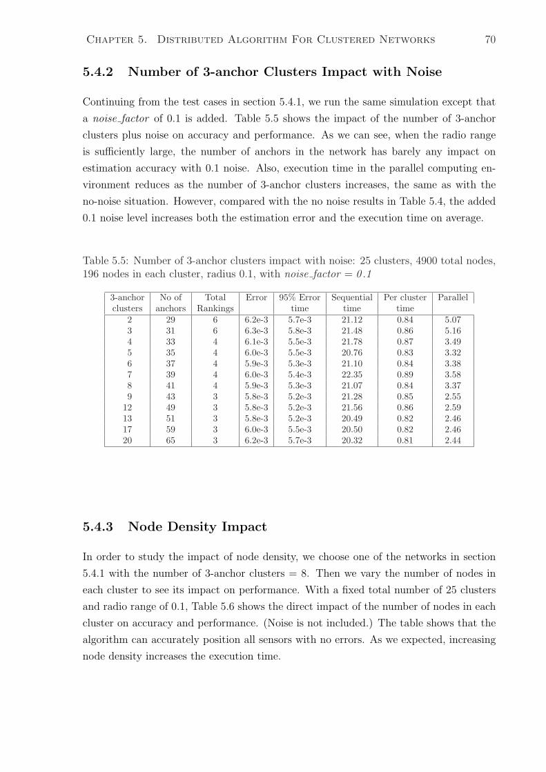
Chapter 5. Distributed Algorithm For Clustered Networks 70
5.4.2 Number of 3-anchor Clusters Impact with Noise
Continuing from the test cases in section 5.4.1, we run the same simulation except that
a noise factor of 0.1 is added. Table 5.5 shows the impact of the number of 3-anchor
clusters plus noise on accuracy and performance. As we can see, when the radio range
is sufficiently large, the number of anchors in the network has barely any impact on
estimation accuracy with 0.1 noise. Also, execution time in the parallel computing en-
vironment reduces as the number of 3-anchor clusters increases, the same as with the
no-noise situation. However, compared with the no noise results in Table 5.4, the added
0.1 noise level increases both the estimation error and the execution time on average.
Table 5.5: Number of 3-anchor clusters impact with noise: 25 clusters, 4900 total nodes,196 nodes in each cluster, radius 0.1, with noise factor = 0 .1
3-anchor No of Total Error 95% Error Sequential Per cluster Parallelclusters anchors Rankings time time time
2 29 6 6.2e-3 5.7e-3 21.12 0.84 5.073 31 6 6.3e-3 5.8e-3 21.48 0.86 5.164 33 4 6.1e-3 5.5e-3 21.78 0.87 3.495 35 4 6.0e-3 5.5e-3 20.76 0.83 3.326 37 4 5.9e-3 5.3e-3 21.10 0.84 3.387 39 4 6.0e-3 5.4e-3 22.35 0.89 3.588 41 4 5.9e-3 5.3e-3 21.07 0.84 3.379 43 3 5.8e-3 5.2e-3 21.28 0.85 2.55
12 49 3 5.8e-3 5.2e-3 21.56 0.86 2.5913 51 3 5.8e-3 5.2e-3 20.49 0.82 2.4617 59 3 6.0e-3 5.5e-3 20.50 0.82 2.4620 65 3 6.2e-3 5.7e-3 20.32 0.81 2.44
5.4.3 Node Density Impact
In order to study the impact of node density, we choose one of the networks in section
5.4.1 with the number of 3-anchor clusters = 8. Then we vary the number of nodes in
each cluster to see its impact on performance. With a fixed total number of 25 clusters
and radio range of 0.1, Table 5.6 shows the direct impact of the number of nodes in each
cluster on accuracy and performance. (Noise is not included.) The table shows that the
algorithm can accurately position all sensors with no errors. As we expected, increasing
node density increases the execution time.
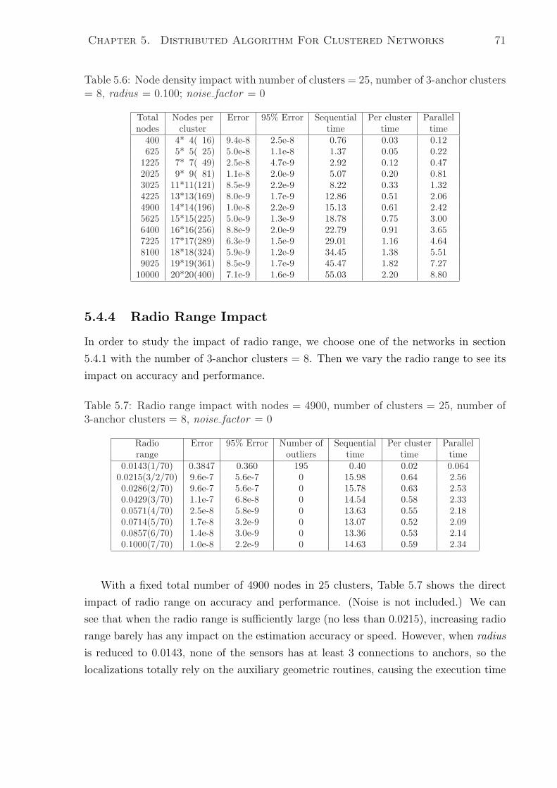
Chapter 5. Distributed Algorithm For Clustered Networks 71
Table 5.6: Node density impact with number of clusters = 25, number of 3-anchor clusters= 8, radius = 0.100; noise factor = 0
Total Nodes per Error 95% Error Sequential Per cluster Parallelnodes cluster time time time
400 4* 4( 16) 9.4e-8 2.5e-8 0.76 0.03 0.12625 5* 5( 25) 5.0e-8 1.1e-8 1.37 0.05 0.22
1225 7* 7( 49) 2.5e-8 4.7e-9 2.92 0.12 0.472025 9* 9( 81) 1.1e-8 2.0e-9 5.07 0.20 0.813025 11*11(121) 8.5e-9 2.2e-9 8.22 0.33 1.324225 13*13(169) 8.0e-9 1.7e-9 12.86 0.51 2.064900 14*14(196) 1.0e-8 2.2e-9 15.13 0.61 2.425625 15*15(225) 5.0e-9 1.3e-9 18.78 0.75 3.006400 16*16(256) 8.8e-9 2.0e-9 22.79 0.91 3.657225 17*17(289) 6.3e-9 1.5e-9 29.01 1.16 4.648100 18*18(324) 5.9e-9 1.2e-9 34.45 1.38 5.519025 19*19(361) 8.5e-9 1.7e-9 45.47 1.82 7.27
10000 20*20(400) 7.1e-9 1.6e-9 55.03 2.20 8.80
5.4.4 Radio Range Impact
In order to study the impact of radio range, we choose one of the networks in section
5.4.1 with the number of 3-anchor clusters = 8. Then we vary the radio range to see its
impact on accuracy and performance.
Table 5.7: Radio range impact with nodes = 4900, number of clusters = 25, number of3-anchor clusters = 8, noise factor = 0
Radio Error 95% Error Number of Sequential Per cluster Parallelrange outliers time time time
0.0143(1/70) 0.3847 0.360 195 0.40 0.02 0.0640.0215(3/2/70) 9.6e-7 5.6e-7 0 15.98 0.64 2.560.0286(2/70) 9.6e-7 5.6e-7 0 15.78 0.63 2.530.0429(3/70) 1.1e-7 6.8e-8 0 14.54 0.58 2.330.0571(4/70) 2.5e-8 5.8e-9 0 13.63 0.55 2.180.0714(5/70) 1.7e-8 3.2e-9 0 13.07 0.52 2.090.0857(6/70) 1.4e-8 3.0e-9 0 13.36 0.53 2.140.1000(7/70) 1.0e-8 2.2e-9 0 14.63 0.59 2.34
With a fixed total number of 4900 nodes in 25 clusters, Table 5.7 shows the direct
impact of radio range on accuracy and performance. (Noise is not included.) We can
see that when the radio range is sufficiently large (no less than 0.0215), increasing radio
range barely has any impact on the estimation accuracy or speed. However, when radius
is reduced to 0.0143, none of the sensors has at least 3 connections to anchors, so the
localizations totally rely on the auxiliary geometric routines, causing the execution time
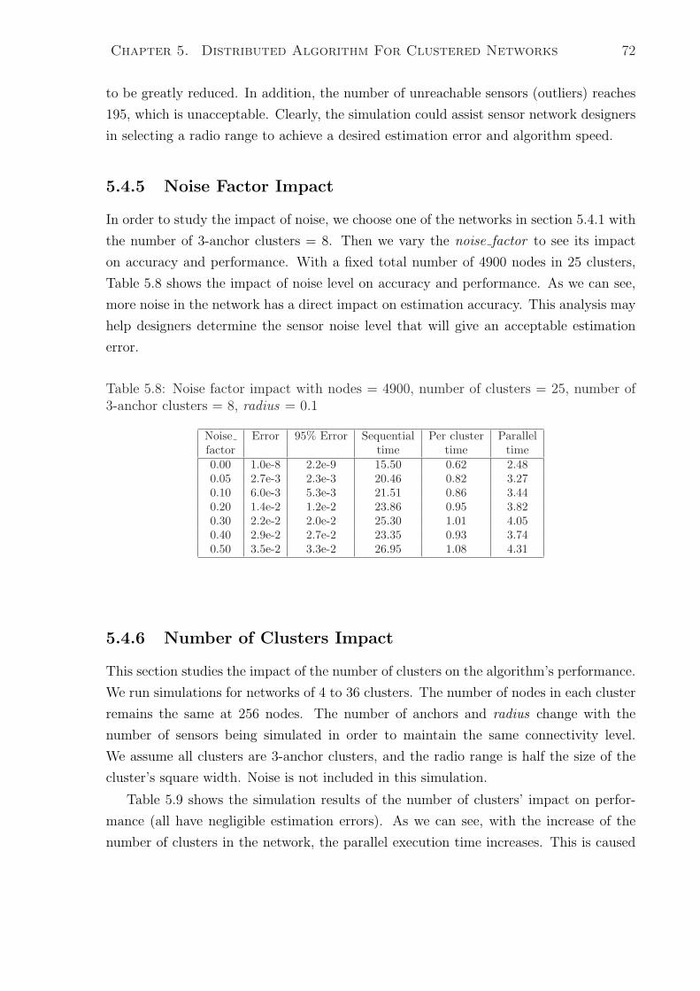
Chapter 5. Distributed Algorithm For Clustered Networks 72
to be greatly reduced. In addition, the number of unreachable sensors (outliers) reaches
195, which is unacceptable. Clearly, the simulation could assist sensor network designers
in selecting a radio range to achieve a desired estimation error and algorithm speed.
5.4.5 Noise Factor Impact
In order to study the impact of noise, we choose one of the networks in section 5.4.1 with
the number of 3-anchor clusters = 8. Then we vary the noise factor to see its impact
on accuracy and performance. With a fixed total number of 4900 nodes in 25 clusters,
Table 5.8 shows the impact of noise level on accuracy and performance. As we can see,
more noise in the network has a direct impact on estimation accuracy. This analysis may
help designers determine the sensor noise level that will give an acceptable estimation
error.
Table 5.8: Noise factor impact with nodes = 4900, number of clusters = 25, number of3-anchor clusters = 8, radius = 0.1
Noise Error 95% Error Sequential Per cluster Parallelfactor time time time0.00 1.0e-8 2.2e-9 15.50 0.62 2.480.05 2.7e-3 2.3e-3 20.46 0.82 3.270.10 6.0e-3 5.3e-3 21.51 0.86 3.440.20 1.4e-2 1.2e-2 23.86 0.95 3.820.30 2.2e-2 2.0e-2 25.30 1.01 4.050.40 2.9e-2 2.7e-2 23.35 0.93 3.740.50 3.5e-2 3.3e-2 26.95 1.08 4.31
5.4.6 Number of Clusters Impact
This section studies the impact of the number of clusters on the algorithm’s performance.
We run simulations for networks of 4 to 36 clusters. The number of nodes in each cluster
remains the same at 256 nodes. The number of anchors and radius change with the
number of sensors being simulated in order to maintain the same connectivity level.
We assume all clusters are 3-anchor clusters, and the radio range is half the size of the
cluster’s square width. Noise is not included in this simulation.
Table 5.9 shows the simulation results of the number of clusters’ impact on perfor-
mance (all have negligible estimation errors). As we can see, with the increase of the
number of clusters in the network, the parallel execution time increases. This is caused
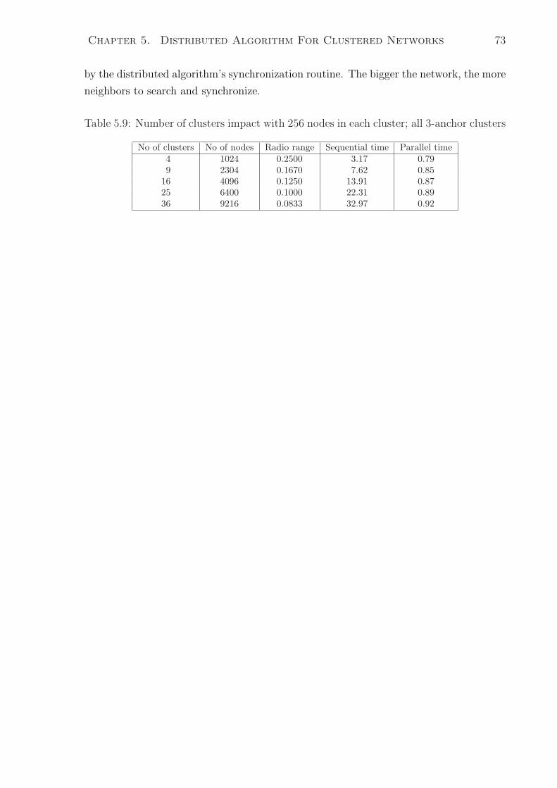
Chapter 5. Distributed Algorithm For Clustered Networks 73
by the distributed algorithm’s synchronization routine. The bigger the network, the more
neighbors to search and synchronize.
Table 5.9: Number of clusters impact with 256 nodes in each cluster; all 3-anchor clusters
No of clusters No of nodes Radio range Sequential time Parallel time4 1024 0.2500 3.17 0.799 2304 0.1670 7.62 0.85
16 4096 0.1250 13.91 0.8725 6400 0.1000 22.31 0.8936 9216 0.0833 32.97 0.92
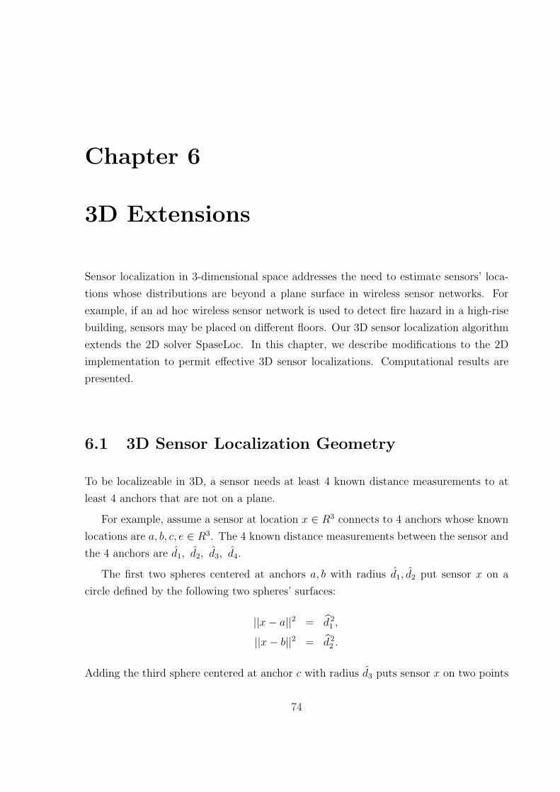
Chapter 6
3D Extensions
Sensor localization in 3-dimensional space addresses the need to estimate sensors’ loca-
tions whose distributions are beyond a plane surface in wireless sensor networks. For
example, if an ad hoc wireless sensor network is used to detect fire hazard in a high-rise
building, sensors may be placed on different floors. Our 3D sensor localization algorithm
extends the 2D solver SpaseLoc. In this chapter, we describe modifications to the 2D
implementation to permit effective 3D sensor localizations. Computational results are
presented.
6.1 3D Sensor Localization Geometry
To be localizeable in 3D, a sensor needs at least 4 known distance measurements to at
least 4 anchors that are not on a plane.
For example, assume a sensor at location x ∈ R3 connects to 4 anchors whose known
locations are a, b, c, e ∈ R3. The 4 known distance measurements between the sensor and
the 4 anchors are d1, d2, d3, d4.
The first two spheres centered at anchors a, b with radius d1, d2 put sensor x on a
circle defined by the following two spheres’ surfaces:
||x− a||2 = d 21 ,
||x− b||2 = d 22 .
Adding the third sphere centered at anchor c with radius d3 puts sensor x on two points
74
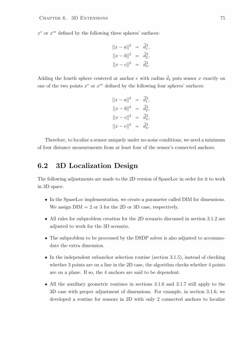
Chapter 6. 3D Extensions 75
x∗ or x∗∗ defined by the following three spheres’ surfaces:
||x− a||2 = d 21 ,
||x− b||2 = d 22 ,
||x− c||2 = d 23 .
Adding the fourth sphere centered at anchor e with radius d4 puts sensor x exactly on
one of the two points x∗ or x∗∗ defined by the following four spheres’ surfaces:
||x− a||2 = d 21 ,
||x− b||2 = d 22 ,
||x− c||2 = d 23 ,
||x− e||2 = d 24 .
Therefore, to localize a sensor uniquely under no-noise conditions, we need a minimum
of four distance measurements from at least four of the sensor’s connected anchors.
6.2 3D Localization Design
The following adjustments are made to the 2D version of SpaseLoc in order for it to work
in 3D space.
• In the SpaseLoc implementation, we create a parameter called DIM for dimensions.
We assign DIM = 2 or 3 for the 2D or 3D case, respectively.
• All rules for subproblem creation for the 2D scenario discussed in section 3.1.2 are
adjusted to work for the 3D scenario.
• The subproblem to be processed by the DSDP solver is also adjusted to accommo-
date the extra dimension.
• In the independent subanchor selection routine (section 3.1.5), instead of checking
whether 3 points are on a line in the 2D case, the algorithm checks whether 4 points
are on a plane. If so, the 4 anchors are said to be dependent.
• All the auxiliary geometric routines in sections 3.1.6 and 3.1.7 still apply to the
3D case with proper adjustment of dimensions. For example, in section 3.1.6, we
developed a routine for sensors in 2D with only 2 connected anchors to localize
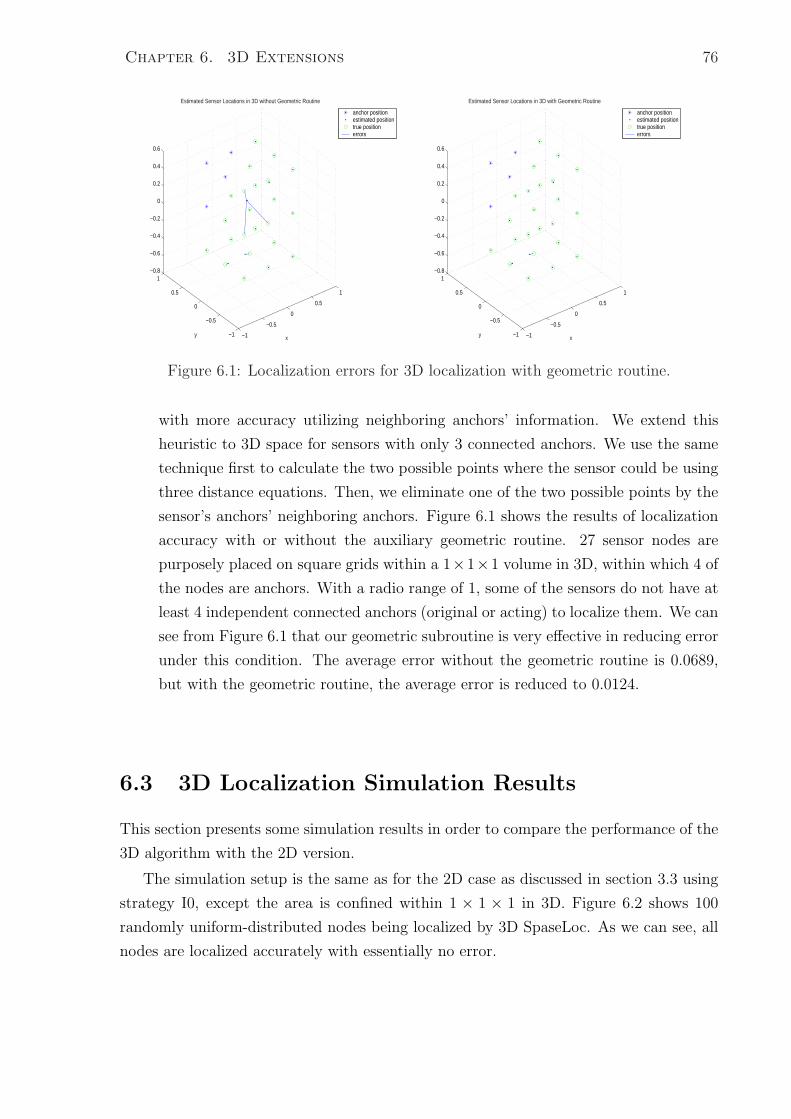
Chapter 6. 3D Extensions 76
−1
−0.5
0
0.5
1
−1
−0.5
0
0.5
1−0.8
−0.6
−0.4
−0.2
0
0.2
0.4
0.6
x
Estimated Sensor Locations in 3D without Geometric Routine
y
anchor positionestimated positiontrue positionerrors
−1
−0.5
0
0.5
1
−1
−0.5
0
0.5
1−0.8
−0.6
−0.4
−0.2
0
0.2
0.4
0.6
x
Estimated Sensor Locations in 3D with Geometric Routine
y
anchor positionestimated positiontrue positionerrors
Figure 6.1: Localization errors for 3D localization with geometric routine.
with more accuracy utilizing neighboring anchors’ information. We extend this
heuristic to 3D space for sensors with only 3 connected anchors. We use the same
technique first to calculate the two possible points where the sensor could be using
three distance equations. Then, we eliminate one of the two possible points by the
sensor’s anchors’ neighboring anchors. Figure 6.1 shows the results of localization
accuracy with or without the auxiliary geometric routine. 27 sensor nodes are
purposely placed on square grids within a 1×1×1 volume in 3D, within which 4 of
the nodes are anchors. With a radio range of 1, some of the sensors do not have at
least 4 independent connected anchors (original or acting) to localize them. We can
see from Figure 6.1 that our geometric subroutine is very effective in reducing error
under this condition. The average error without the geometric routine is 0.0689,
but with the geometric routine, the average error is reduced to 0.0124.
6.3 3D Localization Simulation Results
This section presents some simulation results in order to compare the performance of the
3D algorithm with the 2D version.
The simulation setup is the same as for the 2D case as discussed in section 3.3 using
strategy I0, except the area is confined within 1 × 1 × 1 in 3D. Figure 6.2 shows 100
randomly uniform-distributed nodes being localized by 3D SpaseLoc. As we can see, all
nodes are localized accurately with essentially no error.
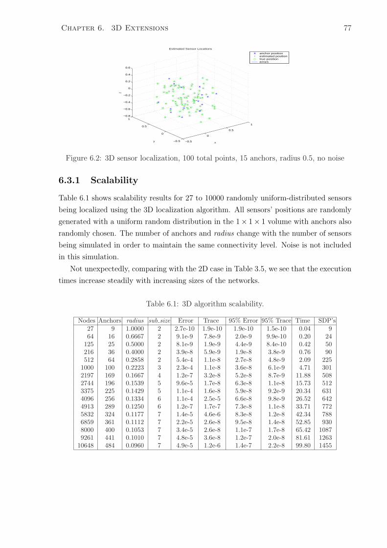
Chapter 6. 3D Extensions 77
−0.5
0
0.5
1
−0.5
0
0.5
1−0.8
−0.6
−0.4
−0.2
0
0.2
0.4
0.6
x
Estimated Sensor Locations
y
z
anchor positionestimated positiontrue positionerrors
Figure 6.2: 3D sensor localization, 100 total points, 15 anchors, radius 0.5, no noise
6.3.1 Scalability
Table 6.1 shows scalability results for 27 to 10000 randomly uniform-distributed sensors
being localized using the 3D localization algorithm. All sensors’ positions are randomly
generated with a uniform random distribution in the 1× 1× 1 volume with anchors also
randomly chosen. The number of anchors and radius change with the number of sensors
being simulated in order to maintain the same connectivity level. Noise is not included
in this simulation.
Not unexpectedly, comparing with the 2D case in Table 3.5, we see that the execution
times increase steadily with increasing sizes of the networks.
Table 6.1: 3D algorithm scalability.
Nodes Anchors radius sub size Error Trace 95% Error 95% Trace Time SDP’s27 9 1.0000 2 2.7e-10 1.9e-10 1.9e-10 1.5e-10 0.04 964 16 0.6667 2 9.1e-9 7.8e-9 2.0e-9 9.9e-10 0.20 24
125 25 0.5000 2 8.1e-9 1.9e-9 4.4e-9 8.4e-10 0.42 50216 36 0.4000 2 3.9e-8 5.9e-9 1.9e-8 3.8e-9 0.76 90512 64 0.2858 2 5.4e-4 1.1e-8 2.7e-8 4.8e-9 2.09 225
1000 100 0.2223 3 2.3e-4 1.1e-8 3.6e-8 6.1e-9 4.71 3012197 169 0.1667 4 1.2e-7 3.2e-8 5.2e-8 8.7e-9 11.88 5082744 196 0.1539 5 9.6e-5 1.7e-8 6.3e-8 1.1e-8 15.73 5123375 225 0.1429 5 1.1e-4 1.6e-8 5.9e-8 9.2e-9 20.34 6314096 256 0.1334 6 1.1e-4 2.5e-5 6.6e-8 9.8e-9 26.52 6424913 289 0.1250 6 1.2e-7 1.7e-7 7.3e-8 1.1e-8 33.71 7725832 324 0.1177 7 1.4e-5 4.6e-6 8.3e-8 1.2e-8 42.34 7886859 361 0.1112 7 2.2e-5 2.6e-8 9.5e-8 1.4e-8 52.85 9308000 400 0.1053 7 3.4e-5 2.6e-8 1.1e-7 1.7e-8 65.42 10879261 441 0.1010 7 4.8e-5 3.6e-8 1.2e-7 2.0e-8 81.61 1263
10648 484 0.0960 7 4.9e-5 1.2e-6 1.4e-7 2.2e-8 99.80 1455
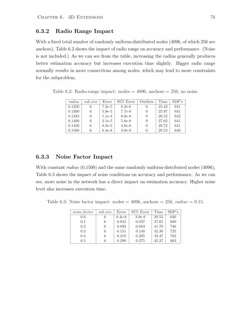
Chapter 6. 3D Extensions 78
6.3.2 Radio Range Impact
With a fixed total number of randomly uniform-distributed nodes (4096, of which 256 are
anchors), Table 6.2 shows the impact of radio range on accuracy and performance. (Noise
is not included.) As we can see from the table, increasing the radius generally produces
better estimation accuracy but increases execution time slightly. Bigger radio range
normally results in more connections among nodes, which may lead to more constraints
for the subproblem.
Table 6.2: Radio-range impact: nodes = 4096, anchors = 256, no noise.
radius sub size Error 95% Error Outliers Time SDP’s0.1250 6 7.2e-5 8.3e-8 0 25.43 6410.1300 6 5.9e-5 7.7e-8 0 25.97 6410.1334 6 1.1e-4 6.6e-8 0 26.52 6420.1400 6 2.1e-5 5.8e-8 0 27.62 6410.1450 6 8.8e-5 4.8e-8 0 28.72 6410.1500 6 6.4e-8 3.9e-8 0 29.53 640
6.3.3 Noise Factor Impact
With constant radius (0.1500) and the same randomly uniform-distributed nodes (4096),
Table 6.3 shows the impact of noise conditions on accuracy and performance. As we can
see, more noise in the network has a direct impact on estimation accuracy. Higher noise
level also increases execution time.
Table 6.3: Noise factor impact: nodes = 4096, anchors = 256, radius = 0.15.
noise factor sub size Error 95% Error Time SDP’s0.0 6 6.4e-8 3.9e-8 29.53 6400.1 6 0.042 0.037 37.65 6800.2 6 0.092 0.083 41.70 7460.3 6 0.151 0.140 42.30 7250.4 6 0.219 0.205 43.47 7030.5 6 0.290 0.275 45.37 663
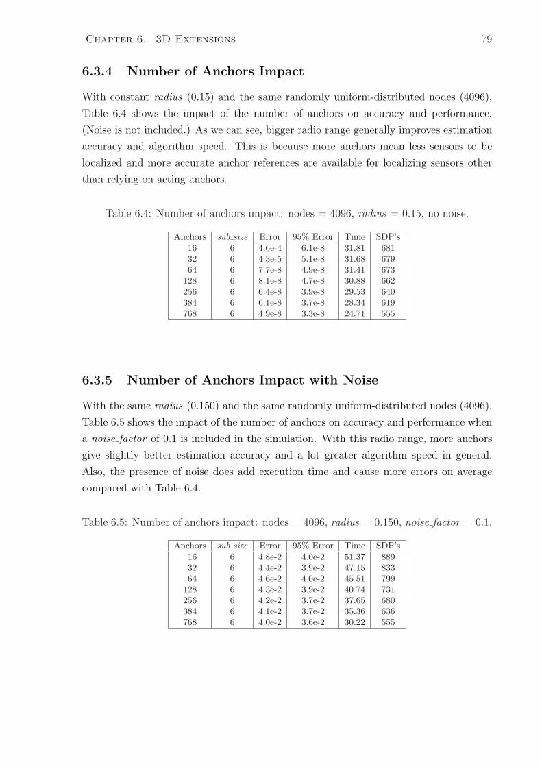
Chapter 6. 3D Extensions 79
6.3.4 Number of Anchors Impact
With constant radius (0.15) and the same randomly uniform-distributed nodes (4096),
Table 6.4 shows the impact of the number of anchors on accuracy and performance.
(Noise is not included.) As we can see, bigger radio range generally improves estimation
accuracy and algorithm speed. This is because more anchors mean less sensors to be
localized and more accurate anchor references are available for localizing sensors other
than relying on acting anchors.
Table 6.4: Number of anchors impact: nodes = 4096, radius = 0.15, no noise.
Anchors sub size Error 95% Error Time SDP’s16 6 4.6e-4 6.1e-8 31.81 68132 6 4.3e-5 5.1e-8 31.68 67964 6 7.7e-8 4.9e-8 31.41 673
128 6 8.1e-8 4.7e-8 30.88 662256 6 6.4e-8 3.9e-8 29.53 640384 6 6.1e-8 3.7e-8 28.34 619768 6 4.9e-8 3.3e-8 24.71 555
6.3.5 Number of Anchors Impact with Noise
With the same radius (0.150) and the same randomly uniform-distributed nodes (4096),
Table 6.5 shows the impact of the number of anchors on accuracy and performance when
a noise factor of 0.1 is included in the simulation. With this radio range, more anchors
give slightly better estimation accuracy and a lot greater algorithm speed in general.
Also, the presence of noise does add execution time and cause more errors on average
compared with Table 6.4.
Table 6.5: Number of anchors impact: nodes = 4096, radius = 0.150, noise factor = 0.1.
Anchors sub size Error 95% Error Time SDP’s16 6 4.8e-2 4.0e-2 51.37 88932 6 4.4e-2 3.9e-2 47.15 83364 6 4.6e-2 4.0e-2 45.51 799
128 6 4.3e-2 3.9e-2 40.74 731256 6 4.2e-2 3.7e-2 37.65 680384 6 4.1e-2 3.7e-2 35.36 636768 6 4.0e-2 3.6e-2 30.22 555
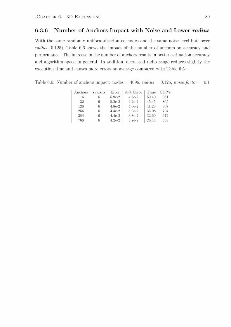
Chapter 6. 3D Extensions 80
6.3.6 Number of Anchors Impact with Noise and Lower radius
With the same randomly uniform-distributed nodes and the same noise level but lower
radius (0.125), Table 6.6 shows the impact of the number of anchors on accuracy and
performance. The increase in the number of anchors results in better estimation accuracy
and algorithm speed in general. In addition, decreased radio range reduces slightly the
execution time and causes more errors on average compared with Table 6.5.
Table 6.6: Number of anchors impact: nodes = 4096, radius = 0.125, noise factor = 0.1
Anchors sub size Error 95% Error Time SDP’s16 6 5.9e-2 4.6e-2 50.40 96132 6 5.2e-2 4.2e-2 45.45 865
128 6 4.8e-2 4.0e-2 41.28 807256 6 4.4e-2 3.9e-2 35.08 704384 6 4.4e-2 3.8e-2 32.60 672768 6 4.2e-2 3.7e-2 26.43 558
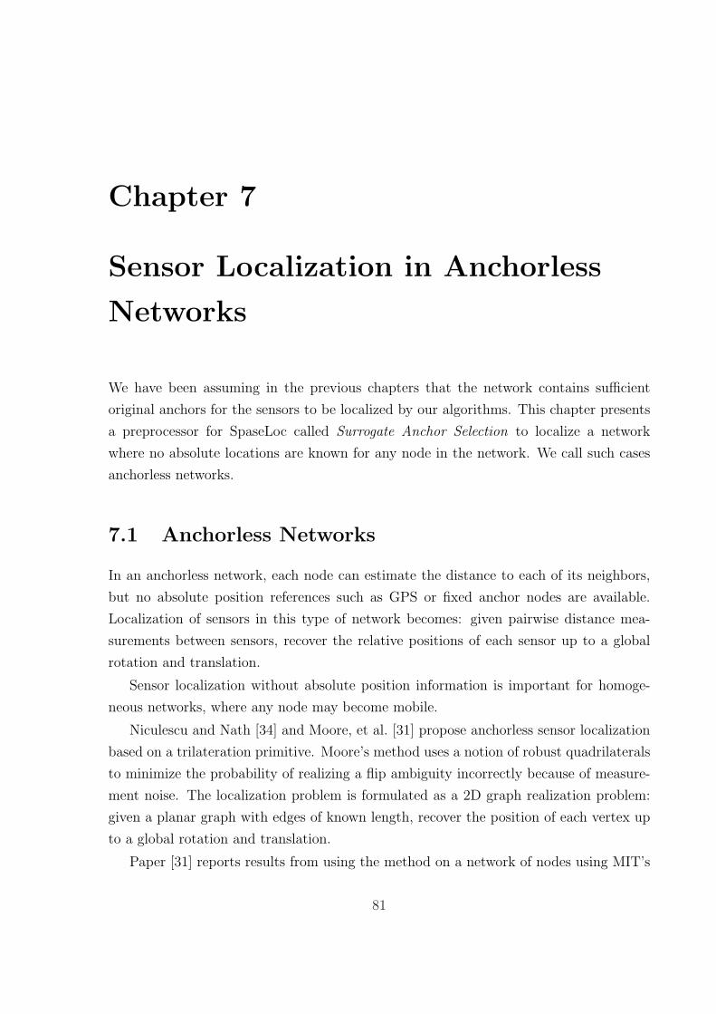
Chapter 7
Sensor Localization in Anchorless
Networks
We have been assuming in the previous chapters that the network contains sufficient
original anchors for the sensors to be localized by our algorithms. This chapter presents
a preprocessor for SpaseLoc called Surrogate Anchor Selection to localize a network
where no absolute locations are known for any node in the network. We call such cases
anchorless networks.
7.1 Anchorless Networks
In an anchorless network, each node can estimate the distance to each of its neighbors,
but no absolute position references such as GPS or fixed anchor nodes are available.
Localization of sensors in this type of network becomes: given pairwise distance mea-
surements between sensors, recover the relative positions of each sensor up to a global
rotation and translation.
Sensor localization without absolute position information is important for homoge-
neous networks, where any node may become mobile.
Niculescu and Nath [34] and Moore, et al. [31] propose anchorless sensor localization
based on a trilateration primitive. Moore’s method uses a notion of robust quadrilaterals
to minimize the probability of realizing a flip ambiguity incorrectly because of measure-
ment noise. The localization problem is formulated as a 2D graph realization problem:
given a planar graph with edges of known length, recover the position of each vertex up
to a global rotation and translation.
Paper [31] reports results from using the method on a network of nodes using MIT’s
81
Chapter 7. Sensor Localization in Anchorless Networks 82
Crickets, which are hardware-compatible with the Mica2 Motes developed at Berkeley
with the addition of an ultrasonic transmitter and receiver on each device. This hardware
enables the sensor nodes to measure inter-node ranges using the time difference of arrival
(TDoA) between ultrasonic and RF signals. Although the Crickets can achieve ranging
precision of around 1cm on the lab bench, the ranging error in practice can be as large
as 5cm because of off-axis alignment of the sending and receiving transducers.
The paper reports experimental results for 16-sensor network localization using the
proposed algorithm. When the measurement errors are averaged at 5.18cm, the algo-
rithm’s localization error is averaged at 7.02cm. The paper also reports simulation results
for bigger networks, and the results of tracking a mobile sensor. There is no report on
the algorithm’s speed.
7.2 Surrogate Anchor Selection
With pairwise distance measurements among sensors and without reference to any ab-
solute positions, we would only be able to determine relative locations of all nodes. The
idea behind our approach is to choose some sensors as reference points (we name these
surrogate anchors), such that the rest of the sensors can be localized relative to these
positions.
We need three surrogate anchors that are not on a line in order to localize the rest of
the sensors uniquely on the plane that the three surrogate anchors are on. (We assume
the network is on a plane. The method can be intuitively expanded to 3D space.)
We define surrogate anchors SA = {a1, a2, a3} in a network to be a subset of sensors
in the same network. Suppose the subset happens to be sensors {s1, s2, s3} with pair-
wise distance measurements d12, d13, d23. These surrogate sensors satisfy the following
properties:
• The first surrogate anchor a1 corresponding to s1 is artificially set to a position of
(0, 0).
• The second surrogate anchor a2 corresponding to s2 is set to a position of (d12, 0).
• The third surrogate anchor a3 corresponding to s3 is set to a position of (x∗x, x∗y),
an intersection of the following two circles:
x2x + x2
y = (d13)2,
(xx − d12)2 + x2
y = (d23)2.

Chapter 7. Sensor Localization in Anchorless Networks 83
Generally there would be two solutions to the above equations. Either one can be
chosen as (x∗x, x∗y).
In this section, we propose a preprocessor to select three sensors to act as surrogate
anchors in the network. SpaseLoc can then be applied to localize the remaining sensor
nodes relative to the surrogate anchors’ positions.
In choosing the surrogate anchors, we give priority to sensors with the highest con-
nectivity to other nodes in the network, in order to reduce transitive errors.
Here are the main steps in the preprocessor for selecting three surrogate anchors.
SA1 Initialize sensor list to include all sensors in the network, and assign sensor list1 =
sensor list.
SA2 For surrogate anchor1, choose the sensor connected to most other sensors in sen-
sor list1, say sensor1.
SA3 For surrogate anchor2, choose sensor2 such that:
– It is connected to surrogate anchor1.
– It is connected to some node sensork that is also connected to surrogate anchor1.
– sensor1, sensor2, and sensork are not on the same line.
If more than one candidate satisfies the above three items, choose the one that has
the most connections to other sensors in sensor list, and set surrogate anchor3 to
be sensork. Go to step SA4.
If there is no candidate satisfying the first three items, delete sensor1 from sen-
sor list1 and return to step SA2.
SA4 Stop.
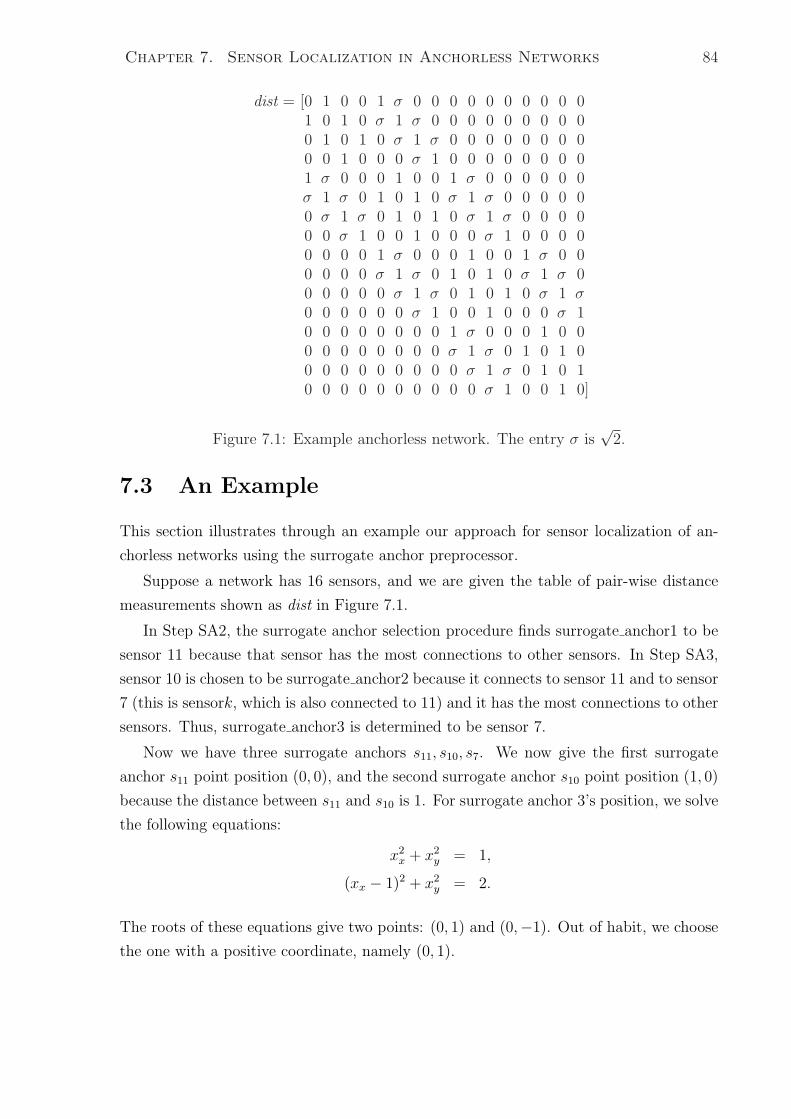
Chapter 7. Sensor Localization in Anchorless Networks 84
dist = [0 1 0 0 1 σ 0 0 0 0 0 0 0 0 0 01 0 1 0 σ 1 σ 0 0 0 0 0 0 0 0 00 1 0 1 0 σ 1 σ 0 0 0 0 0 0 0 00 0 1 0 0 0 σ 1 0 0 0 0 0 0 0 01 σ 0 0 0 1 0 0 1 σ 0 0 0 0 0 0σ 1 σ 0 1 0 1 0 σ 1 σ 0 0 0 0 00 σ 1 σ 0 1 0 1 0 σ 1 σ 0 0 0 00 0 σ 1 0 0 1 0 0 0 σ 1 0 0 0 00 0 0 0 1 σ 0 0 0 1 0 0 1 σ 0 00 0 0 0 σ 1 σ 0 1 0 1 0 σ 1 σ 00 0 0 0 0 σ 1 σ 0 1 0 1 0 σ 1 σ0 0 0 0 0 0 σ 1 0 0 1 0 0 0 σ 10 0 0 0 0 0 0 0 1 σ 0 0 0 1 0 00 0 0 0 0 0 0 0 σ 1 σ 0 1 0 1 00 0 0 0 0 0 0 0 0 σ 1 σ 0 1 0 10 0 0 0 0 0 0 0 0 0 σ 1 0 0 1 0]
Figure 7.1: Example anchorless network. The entry σ is√
2.
7.3 An Example
This section illustrates through an example our approach for sensor localization of an-
chorless networks using the surrogate anchor preprocessor.
Suppose a network has 16 sensors, and we are given the table of pair-wise distance
measurements shown as dist in Figure 7.1.
In Step SA2, the surrogate anchor selection procedure finds surrogate anchor1 to be
sensor 11 because that sensor has the most connections to other sensors. In Step SA3,
sensor 10 is chosen to be surrogate anchor2 because it connects to sensor 11 and to sensor
7 (this is sensork, which is also connected to 11) and it has the most connections to other
sensors. Thus, surrogate anchor3 is determined to be sensor 7.
Now we have three surrogate anchors s11, s10, s7. We now give the first surrogate
anchor s11 point position (0, 0), and the second surrogate anchor s10 point position (1, 0)
because the distance between s11 and s10 is 1. For surrogate anchor 3’s position, we solve
the following equations:
x2x + x2
y = 1,
(xx − 1)2 + x2y = 2.
The roots of these equations give two points: (0, 1) and (0,−1). Out of habit, we choose
the one with a positive coordinate, namely (0, 1).
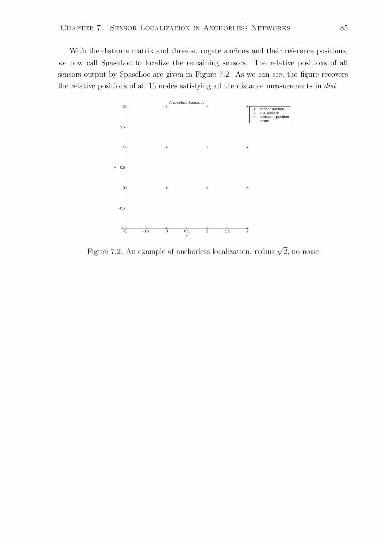
Chapter 7. Sensor Localization in Anchorless Networks 85
With the distance matrix and three surrogate anchors and their reference positions,
we now call SpaseLoc to localize the remaining sensors. The relative positions of all
sensors output by SpaseLoc are given in Figure 7.2. As we can see, the figure recovers
the relative positions of all 16 nodes satisfying all the distance measurements in dist.
−1 −0.5 0 0.5 1 1.5 2−1
−0.5
0
0.5
1
1.5
2
x
y
Anchorless SpaseLoc
anchor positiontrue positionestimated positionerrors
Figure 7.2: An example of anchorless localization, radius√
2, no noise
Chapter 8
Conclusions and Future Research
In this dissertation research, we have developed a range of algorithms to estimate sensor
positions in static, dynamic, distributed, 2D and 3D wireless sensor networks. This
chapter summarizes the proposed approaches and discusses future research directions.
8.1 Contributions
The proposed algorithms achieve a breakthrough in scalability and accuracy compared
with existing methods. The advances were recognized when this research project tied for
first prize in the 2005 Stanford-Berkeley Innovators’ Challenge competition. All entries
were judged in the categories of Technical Innovation, Execution, and Future Impact [25].
Existing localization methods have been applicable for only moderate-sized networks.
The recent optimization approach by Biswas and Ye [4] uses semidefinite programming
(SDP) to find an approximate solution. This is a vital tool, but its speed and accuracy
deteriorate rapidly with network size. The computational complexity of this approach is
O(np), where p is between 3 and 4.
The complexity of our SpaseLoc algorithm is O(n). On a 2.4GHz laptop with 1GB
memory, the algorithm maintains efficiency and provides accurate position estimation for
networks with 10000 sensors and beyond.
SpaseLoc is further utilized as a vital tool for more general localization algorithms.
A dynamic version can estimate moving sensors’ locations in real-time, and a 3D version
extends its utility. We also deploy SpaseLoc in clustered and distributed environments,
permitting application to arbitrarily large networks.
Figure 8.1 compares the localization results between our SpaseLoc algorithm and the
pure SDP approach for various size networks. The left-hand figure shows a comparison
86
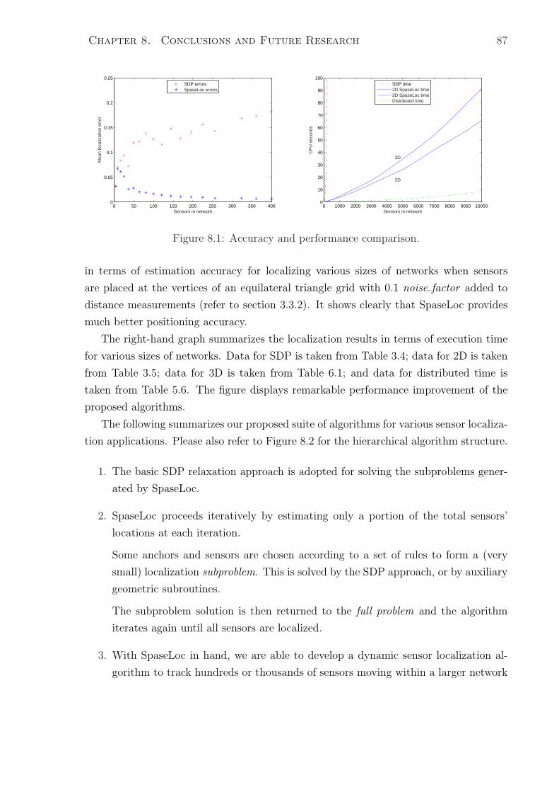
Chapter 8. Conclusions and Future Research 87
0 50 100 150 200 250 300 350 4000
0.05
0.1
0.15
0.2
0.25
Sensors in network
Mea
n lo
caliz
atio
n er
ror
SDP errorsSpaseLoc errors
0 1000 2000 3000 4000 5000 6000 7000 8000 9000 100000
10
20
30
40
50
60
70
80
90
100
Sensors in network
CP
U s
econ
ds
2D
3D
SDP time2D SpaseLoc time3D SpaseLoc timeDistributed time
Figure 8.1: Accuracy and performance comparison.
in terms of estimation accuracy for localizing various sizes of networks when sensors
are placed at the vertices of an equilateral triangle grid with 0.1 noise factor added to
distance measurements (refer to section 3.3.2). It shows clearly that SpaseLoc provides
much better positioning accuracy.
The right-hand graph summarizes the localization results in terms of execution time
for various sizes of networks. Data for SDP is taken from Table 3.4; data for 2D is taken
from Table 3.5; data for 3D is taken from Table 6.1; and data for distributed time is
taken from Table 5.6. The figure displays remarkable performance improvement of the
proposed algorithms.
The following summarizes our proposed suite of algorithms for various sensor localiza-
tion applications. Please also refer to Figure 8.2 for the hierarchical algorithm structure.
1. The basic SDP relaxation approach is adopted for solving the subproblems gener-
ated by SpaseLoc.
2. SpaseLoc proceeds iteratively by estimating only a portion of the total sensors’
locations at each iteration.
Some anchors and sensors are chosen according to a set of rules to form a (very
small) localization subproblem. This is solved by the SDP approach, or by auxiliary
geometric subroutines.
The subproblem solution is then returned to the full problem and the algorithm
iterates again until all sensors are localized.
3. With SpaseLoc in hand, we are able to develop a dynamic sensor localization al-
gorithm to track hundreds or thousands of sensors moving within a larger network
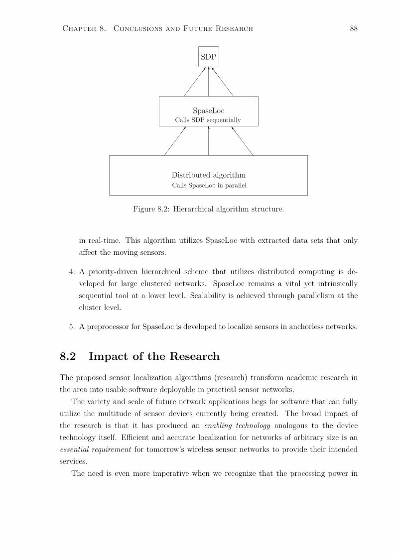
Chapter 8. Conclusions and Future Research 88
SDP
SpaseLoc
Distributed algorithm
Calls SDP sequentially
Calls SpaseLoc in parallel
¶¶
¶¶¶7 6
SS
SSSo
¶¶
¶¶¶7 6
SS
SSSo
Figure 8.2: Hierarchical algorithm structure.
in real-time. This algorithm utilizes SpaseLoc with extracted data sets that only
affect the moving sensors.
4. A priority-driven hierarchical scheme that utilizes distributed computing is de-
veloped for large clustered networks. SpaseLoc remains a vital yet intrinsically
sequential tool at a lower level. Scalability is achieved through parallelism at the
cluster level.
5. A preprocessor for SpaseLoc is developed to localize sensors in anchorless networks.
8.2 Impact of the Research
The proposed sensor localization algorithms (research) transform academic research in
the area into usable software deployable in practical sensor networks.
The variety and scale of future network applications begs for software that can fully
utilize the multitude of sensor devices currently being created. The broad impact of
the research is that it has produced an enabling technology analogous to the device
technology itself. Efficient and accurate localization for networks of arbitrary size is an
essential requirement for tomorrow’s wireless sensor networks to provide their intended
services.
The need is even more imperative when we recognize that the processing power in
Chapter 8. Conclusions and Future Research 89
sensor devices of the near future will be far less than a current Pentium laptop. SpaseLoc
is already a major advance for networks up to ten thousands nodes. The distributed
algorithm takes a further quantum leap by attaining true scalability and deployability.
8.3 Future Research
We are actively pursuing extensions of the sensor localization algorithms. The following
are some promising directions.
Molecular structure identification
In biotechnology, there exist ways to obtain clustered pairwise distance measurements
between atoms inside a molecule. The problem then is how to deduce the molecular
structure utilizing these known distance measurements, so the molecule’s characteristics
can be further analyzed. This molecular structure identification problem [47, 48] is very
similar in form to the geometric distance model for sensor localization. The protein
folding problem [1, 10, 32, 35] and the Euclidean Distance Matrix problem [49, 50] are
also closely related. We plan to expand our method to be applicable to these areas.
Cartography
A classical paper by Gauss [16] describes a least-squares approach to constructing a map
of Holland using pairwise distance measurements between neighboring villages. This is
closely related to the sensor localization problem. The distance matrix is sparse, and
the required solution is in 3D (to allow for curvature of the earth). We plan to explore
applying our method to this problem.
General version of distributed algorithm
We are currently working on generalizing our distributed approach to arbitrary topologies.
In the future, we plan to utilize Stanford’s Sweet Hall computer clusters to implement
our distributed algorithm to achieve true parallel computing.
Objective function with `2 norm
This thesis reports results from formulating the sensor localization problem as in (2.1):
minimizing the `1 norm of the squared-distance errors αij and αik. The localization
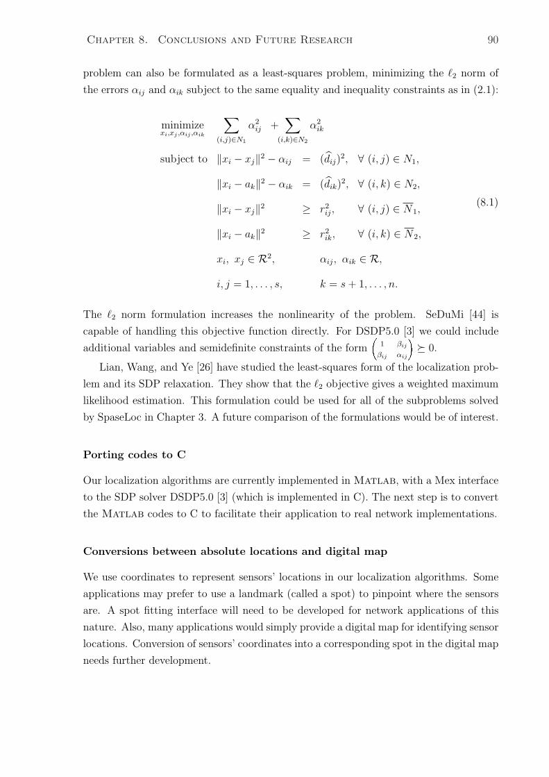
Chapter 8. Conclusions and Future Research 90
problem can also be formulated as a least-squares problem, minimizing the `2 norm of
the errors αij and αik subject to the same equality and inequality constraints as in (2.1):
minimizexi,xj ,αij ,αik
∑
(i,j)∈N1
α2ij +
∑
(i,k)∈N2
α2ik
subject to ‖xi − xj‖2 − αij = (dij)2, ∀ (i, j) ∈ N1,
‖xi − ak‖2 − αik = (dik)2, ∀ (i, k) ∈ N2,
‖xi − xj‖2 ≥ r2ij, ∀ (i, j) ∈ N1,
‖xi − ak‖2 ≥ r2ik, ∀ (i, k) ∈ N2,
xi, xj ∈ R2, αij, αik ∈ R,
i, j = 1, . . . , s, k = s + 1, . . . , n.
(8.1)
The `2 norm formulation increases the nonlinearity of the problem. SeDuMi [44] is
capable of handling this objective function directly. For DSDP5.0 [3] we could include
additional variables and semidefinite constraints of the form
1 βij
βij αij
!º 0.
Lian, Wang, and Ye [26] have studied the least-squares form of the localization prob-
lem and its SDP relaxation. They show that the `2 objective gives a weighted maximum
likelihood estimation. This formulation could be used for all of the subproblems solved
by SpaseLoc in Chapter 3. A future comparison of the formulations would be of interest.
Porting codes to C
Our localization algorithms are currently implemented in Matlab, with a Mex interface
to the SDP solver DSDP5.0 [3] (which is implemented in C). The next step is to convert
the Matlab codes to C to facilitate their application to real network implementations.
Conversions between absolute locations and digital map
We use coordinates to represent sensors’ locations in our localization algorithms. Some
applications may prefer to use a landmark (called a spot) to pinpoint where the sensors
are. A spot fitting interface will need to be developed for network applications of this
nature. Also, many applications would simply provide a digital map for identifying sensor
locations. Conversion of sensors’ coordinates into a corresponding spot in the digital map
needs further development.

Chapter 8. Conclusions and Future Research 91
Deployment to real-world applications
We are currently developing collaborations with several companies with the aim of ap-
plying our algorithms to real-world applications.
Bibliography
[1] A. Alfakih, A. Khandani, and H. Wolkowicz. Solving Euclidean distance matrix
completion problems via semidefinite programming, Comput. Optim. Appl., 12(1–3) (1999),
pp. 13–30. Computational optimization—a tribute to Olvi Mangasarian, Part I.
[2] P. Bahl and V. N. Padmanabhan. RADAR: An In-Building RF-Based User Location
and Tracking System, Proceedings of IEEE INFOCOM 2000, Vol. 2, Tel-Aviv, Israel,
March 2000, pp. 775–784
[3] S. J. Benson, Y. Ye, and X. Zhang. DSDP, http://www-unix.mcs.anl.gov/˜benson/
or http://www.stanford.edu/˜yyye/Col.html, 1998–2005.
[4] P. Biswas and Y. Ye. Semidefinite programming for ad hoc wireless sensor network
localization, IPSN 2004, Berkeley, CA, April 26–27, 2004.
[5] P. Biswas and Y. Ye. A distributed method for solving semidefinite programs arising
from ad hoc wireless sensor network localization, Working Paper, Departments of EE and
MS&E, Stanford University, CA, October 30, 2003.
[6] S. Boyd, L. El Ghaoui, E. Feron, and V. Balakrishnan. Linear Matrix Inequalities
in System and Control Theory, SIAM, Philadelphia, 1994.
[7] N. Bulusu, J. Heidemann, and D. Estrin. GPS-less low cost outdoor localization for
very small devices, Technical Report 00-729, Computer Science Department, University of
Southern California, CA, April 2000.
[8] S. Capkun, M. Hamdi, and J. P. Hubaux. GPS-free positioning in mobile ad-hoc
networks. Procedings of the 34th Hawaii International Conference on System Sciences,
2001.
[9] A. Cha. Electronic tracking is finding new uses, San Jose Mercury News, Sunday, Jan.
16, 2005.
[10] G. M. Crippen and T. F. Havel, Distance Geometry and Molecular Conformation,
Wiley, New York, 1988.
92
BIBLIOGRAPHY 93
[11] D. Culler and W. Hong. Wireless sensor networks. Communications of the ACM,
47(6), June 2004, pp. 30–33.
[12] L. Doherty, L. El Ghaoui, and K. Pister. Convex position estimation in wireless
sensor networks. Proc. IEEE Infocom 2001, Anchorage, AK, April 2001, pp. 1655–1663.
[13] A. Dragoon. Small wonders. CIO Magazine, January 15, 2005.
[14] W. Drozdiak. Automotive alternative: In German Port City, cheap, efficient car rentals
catch on, Washington Post, September 20, 1999, p. A09.
[15] D. Ganesan, B. Krishnamachari, A. Woo, D. Culler, D. Estrin, and S. Wicker.
An empirical study of epidemic algorithms in large-scale multihop wireless networks. Re-
port UCLA/CSD-TR-02-0013, Computer Science Department, UCLA, CA, 2002.
[16] C. F. Gauss. Gauss’s work (1803–1826) on the theory of least squares: an English trans-
lation by Hale F. Trotter, QA 275.G3, 1957.
[17] G. H. Golub and C. F. Van Loan. Matrix Computations, The Johns Hopkins University
Press, Baltimore, MD, 3rd edition, 1996.
[18] W. B. Heinzelman, A. P. Chandrakasan, and H. Balakrishnan. An application-
specific protocol architecture for wireless microsensor networks, IEEE Transactions on
Wireless Communications, 1(4) (October 2002).
[19] J. Hightower and G. Boriello. Location systems for ubiquitous computing, IEEE
Computer, 34(8) (2001), pp. 57–66.
[20] A. Howard, M. J. Mataric, and G. S. Sukhatme. Relaxation on a mesh: a formalism
for generalized localization, in Proc. IEEE/RSJ International Conf. on Intelligent Robots
and Systems (IROS01), 2001, pp. 1055–1060.
[21] H. H. Jin, M. W. Carter, M. A. Saunders, and Y. Ye. SpaseLoc: An adaptive
subproblem algorithm for scalable wireless sensor network localization, SIAM J. on Opti-
mization, submitted December 2004.
[22] H. H. Jin, M. W. Carter, and M. A. Saunders. Moving sensors localizations, pre-
sented at INFORMS Annual Meeting, Denver, October 23–27, 2004.
[23] H. H. Jin, M. W. Carter, and M. A. Saunders. Sensors localization in 3D, presented
at SIAM Conference on Optimization, Stockholm, Sweden, May 15–19, 2005.
[24] H. H. Jin, M. W. Carter, and M. A. Saunders. Distributed algorithm for sensor
localization, presented at IFORS Triennial International Conf., Hawaii, July 11–15, 2005.
BIBLIOGRAPHY 94
[25] H. H. Jin, M. W. Carter, M. A. Saunders, and Y. Ye. Scalable algorithms for
sensor localization, first-equal prize winner at the Stanford-Berkeley Innovators’ Challenge
competition, Stanford University, April 19, 2005.
[26] T.-C. Liang, T.-C. Wang, and Y. Ye. Semidefinite programming relaxation solution
for ad hoc wireless sensor network localization, Technical Report, Stanford University,
October 1, 2004.
[27] M. Lawlor. Small systems, big business, Signal Magazine, January 2005.
[28] X. Y. Lu. Coordination layer control and decision making for automated ground vehicles,
Proceedings of the American Control Conf., Anchorage, May 8–10, 2002, pp. 3034–3039.
[29] Matlab 6.5, Release 13 with Service Pack 1. The MathWorks, Inc., Natick, MA, 2003.
[30] A. F. McMillan. Car sharing’s time comes, CNN Money, July 19, 2000.
[31] D. Moore, J. Leonard, D. Rus, and Seth Teller. Robust Distributed Network Lo-
calization with Noisy Range Measurements, SenSys04, November 3–5, 2004, Baltimore,
Maryland, USA.
[32] J. J. More and Z. Wu. Distance geometry optimization for protein structures, J. Global
Optim., 15(3) (1999), pp. 219–234.
[33] D. Niculescu and B. Nath. Ad hoc positioning system, IEEE GlobeCom, November
2001, pp. 2926–2931.
[34] D. Niculescu and B. Nath. DV based positioning in ad hoc networks, Kluwer Journal
of Telecommunicaton Systems, 2003, pp. 267–280.
[35] R. Reams, G. Chatham, W. Glunt, D. McDonald, and T. Hayden. Determining
protein structure using the distance geometry program apa, Computers and Chemistry, 23
(1999), pp. 153–163.
[36] A. Ricadela. Sensors everywhere, Information Week, January 24, 2005.
[37] C. Savarese, J. Rabaey, and K. Langendoen. Robust positioning algorithm for dis-
tributed ad hoc wireless sensor networks, in USENIX Technical Annual Conf., Monterey,
CA, June 2002.
[38] A. Savvides, C.-C. Han, and M. B. Srivastava. Dynamic fine-grained localization in
ad hoc networks of sensors, in ACM/IEEE International Conf. on Mobile Computing and
Networking (MOBICON), July 2001, pp. 166–179.
BIBLIOGRAPHY 95
[39] A. Savvides, H. Park, and M. B. Srivastava. The bits and flops of the n-hop multi-
lateration primitive for node localization problems, in 1st ACM International Workshop on
Wireless Sensor Networks and Applications (WSNA’02), Atlanta, GA, 2002, ACM Press,
pp. 112–121.
[40] Y. Shang, W. Ruml, Y. Zhang, and M. Fromherz. Localization from mere connec-
tivity, MobiHoc 2003, Anapolis, MD, June 2003, ACM Press.
[41] S. Shladover, and P. Ioannou. Reasons for operating AHS vehicles in platoons, Au-
tomated Highway Systems, Klumer Academic/Plenum Publishers, New York, 1997, pp.
11–28.
[42] J. P. Singh, N. Bambos, B. Srinivasan, and D. Clawin. Wireless LAN performance
under varied stress conditions in vehicular traffic scenarios, Technical Report, Depart-
ment of Electrical Engineering, Stanford University, CA, and Robert Bosch Coorporation,
Research and Technology Center, Palo Alto, CA.
[43] A. So and Y. Ye. Theory of semidefinite programming for sensor network localization,
Stanford University, CA, 2004, to appear in SODA 2005.
[44] J. F. Sturm. Let SeDuMi seduce you, http://fewcal.kub.nl/sturm/software/sedumi.html,
October 2001.
[45] R. Szewczyk, E. Osterweil, J. Polastre, M. Hamilton, A. Mainwaring, and D.
Estrin. Habitat monitoring with sensor networks. Communications of the ACM, 47(6),
June 2004, pp. 34–44.
[46] P. Tseng. SOCP relaxation for nonconvex optimization, presented at ICCOPT 1, RPI,
Troy, NY, August 2–5, 2004.
[47] G. A. Williams, J. M. Dugan, and R. B. Altman, Constrained global optimization for
estimating molecular structure from atomic distances, J. Computational Biology, 8 (2001),
pp. 523-547.
[48] D. Wu and Z. Wu, An updated geometric build-up algorithm for molecular distance
geometry problems with sparse distance data, preprint, University of Iowa, 2005.
[49] F. Z. Zhang. On the best Euclidean fit to a distance matrix, Beijing Shifan Daxue Xuebao,
4 (1987), pp. 21–24.
[50] Z. Zou, R. H. Byrd, and R. B. Schnabel. A stochastic/perturbation global optimiza-
tion algorithm for distance geometry problems, Technical Report, Dept. of Computer Sci-
ence, University of Colorado, Boulder, CO, 1996.