Wind Information Requirements for NextGen Applications ... · 2 Wind Information Analysis Framework 2! 3 4D-TBO Challenging Wind Environments 6! 4 Wind Metric and ATC/Wind Scenario

Lincoln Laboratory MASSACHUSETTS INSTITUTE OF TECHNOLOGY

LEXINGTON, MASSACHUSETTS

Project Report ATC-418

Wind Information Requirements for NextGen Applications

Phase 2 Final Report: Framework

Refinement and Application to Four-Dimensional Trajectory Based Operations (4D-TBO) and Interval Management (IM)

T.G. Reynolds

P.M. Lamey M.D. McPartland

M.J. Sandberg

T.L. Teller S.W. Troxel

Y. Glina

May 2014

Prepared for the Federal Aviation Administration, Washington, D.C. 20591

This document is available to the public through the National Technical Information Service,

Springfield, Virginia 22161

This document is disseminated under the sponsorship of the Department of Transportation, Federal Aviation Administration, in the interest of information exchange. The United States Government assumes no liability for its contents or use thereof.

17. Key Words 18. Distribution Statement

19. Security Classif. (of this report) 20. Security Classif. (of this page) 21. No. of Pages 22. Price

TECHNICAL REPORT STANDARD TITLE PAGE

1. Report No. 2. Government Accession No. 3. Recipient's Catalog No.

4. Title and Subtitle 5. Report Date

6. Performing Organization Code

7. Author(s) 8. Performing Organization Report No.

9. Performing Organization Name and Address 10. Work Unit No. (TRAIS)

11. Contract or Grant No.

12. Sponsoring Agency Name and Address 13. Type of Report and Period Covered

14. Sponsoring Agency Code

15. Supplementary Notes

16. Abstract

Unclassified Unclassified 74

FORM DOT F 1700.7 (8-72) Reproduction of completed page authorized

T.G. Reynolds, P.M. Lamey, M.D. McPartland, M.J. Sandberg, T.L. Teller, S. Troxel, and Y. Glina, MIT Lincoln Laboratory

MIT Lincoln Laboratory 244 Wood Street Lexington, MA 02420-9108

This report is based on studies performed at Lincoln Laboratory, a federally funded research and development center operated by Massachusetts Institute of Technology, under Air Force Contract FA8721-05-C-0002.

This document is available to the public through the National Technical Information Service, Springfield, VA 22161.

ATC-418

Wind Information Requirements for NextGen Applications Phase 2 Final Report: Framework Refinement and Application to Four-Dimensional Trajectory Based Operations (4D-TBO) and Interval Management (IM)

Department of Transportation Federal Aviation Administration 800 Independence Ave., S.W. Washington, DC 20591

Project Report

ATC-418

TBD 2014

Accurate wind information is of fundamental importance to some of the critical future air traffic concepts envisioned under the FAA’s Next Generation Air Transportation System (NextGen) initiative. Concepts involving time elements, such as Four-Dimensional Trajectory Based Operations (4D-TBO) and Interval Management (IM), are especially sensitive to wind information accuracy. There is a growing need to establish appropriate concepts of operation and target performance requirements accounting for wind information accuracy for these types of procedure, and meeting these needs is the purpose of this project.

In the first phase of this work, a Wind Information Analysis Framework was developed to help explore the relationship of wind information to NextGen application performance. A refined version of the framework has been developed for the Phase 2 work that highlights the role stakeholders play in defining Air Traffic Control (ATC) scenarios, distinguishes wind scenarios into benign, moderate, severe, and extreme categories, and more clearly identifies what and how wind requirements recommendations are developed from the performance assessment trade-spaces. This report documents how this refined analysis framework has been used in Phase 2 of the work in terms of:

• RefinedwindinformationmetricsandwindscenarioselectionprocessapplicabletoabroaderrangeofNextGenapplications,withparticular focus on 4D-TBO and IM.

• Expandedandrefinedstudiesof4D-TBOapplicationswithcurrentFlightManagementSystems(FMS)(withMITREcollaboration)to identify more accurate trade-spaces using operational FMS capabilities with higher-fidelity aircraft models.

• Expansionofthe4D-TBOstudyusingincrementalenhancementspossibleinfutureFMSs(withHoneywellcollaboration),specificallyin the area of wind blending algorithms to quantify performance improvement potential from near-term avionics refinements.

• DemonstratingtheadaptabilityoftheWindInformationAnalysisFrameworkbyusingittoidentifyinitialwindinformationneedsfor IM applications.

FA8721-05-C-0002

This page intentionally left blank.

iii

REVISION HISTORY

Version Description Release Date 0.1 Draft version of Interim Phase 2 Final Report 11/15/13 0.2 Internal working version N/A 0.3 Second draft release version with draft content for all sections 1/24/14 0.4 Revised complete draft for sponsor approval prior to release 3/27/14 1.0 Release version after comment period 4/25/14


v

EXECUTIVE SUMMARY

Accurate wind information is of fundamental importance to some of the critical future air traffic concepts envisioned under the FAA’s Next Generation Air Transportation System (NextGen) initiative. Concepts involving time elements, such as Four-Dimensional Trajectory Based Operations (4D-TBO) and Interval Management (IM), are especially sensitive to wind information accuracy. There is a growing need to establish appropriate concepts of operation and target performance requirements accounting for wind information accuracy for these types of procedure, and meeting these needs is the purpose of this project.

In the first phase of this work, a Wind Information Analysis Framework was developed to help explore the relationship of wind information to NextGen application performance. A refined version of the framework has been developed for the Phase 2 work that highlights the role stakeholders play in defining Air Traffic Control (ATC) scenarios, distinguishes wind scenarios into benign, moderate, severe, and extreme categories, and more clearly identifies what and how wind requirements recommendations are developed from the performance assessment trade-spaces. This report documents how this refined analysis framework has been used in Phase 2 of the work in terms of:

• Refined wind information metrics and wind scenario selection process applicable to a broader range of NextGen applications, with particular focus on 4D-TBO and IM.

• Expanded and refined studies of 4D-TBO applications with current Flight Management Systems (FMS) (with MITRE collaboration) to identify more accurate trade-spaces using operational FMS capabilities with higher-fidelity aircraft models.

• Expansion of the 4D-TBO study using incremental enhancements possible in future FMSs (with Honeywell collaboration), specifically in the area of wind blending algorithms to quantify performance improvement potential from near-term avionics refinements.

• Demonstrating the adaptability of the Wind Information Analysis Framework by using it to

identify initial wind information needs for IM applications.

In terms of refined wind information metrics and wind scenario selection processes, comparisons of operational wind forecast models have been updated given latest information and expanded to cover more models used in the aviation community. A general process model is developed that shows the importance of understanding the Concept of Operation, aircraft and ground capabilities in the selection of appropriate wind metrics of interest for a given NextGen application, which can then be used to identify appropriate truth and forecast wind scenarios. Two truth wind scenario selection approaches (volumetric and trajectory-based) are described and illustrated. Simulating realistic wind forecast errors is described using techniques that respect the magnitude of Root Means Square (RMS) error and spatial/temporal correlation

vi

characteristics seen in the operational wind forecast models used in the aviation domain. Moving forward, Phase 3 work will examine refinements to the trajectory-based wind scenario selection approach, which not only account for the aggregate wind characteristics along a given trajectory, but also where they occur along the trajectory. Such an approach could distinguish between wind variability and forecast error location relative to the meter fix location and therefore allow an assessment of this potentially important performance driver.

In terms of expanded and refined studies of 4D-TBO applications with current FMSs, high fidelity simulation activities using operational FMS hardware have been used to identify key variables that impact Required Time of Arrival (RTA) compliance performance, and then developing trade-spaces to understand the relationship of those variables, RTA performance and wind information accuracy. The main objective for Phase 3 is to develop sets of refined trade-spaces relating RTA compliance performance to major performance drivers for multiple aircraft/FMS equipment combinations across a broader range of operational conditions than was possible in Phase 2. Once the refined trade-spaces have been defined, additional steps will be conducted in Phase 3 to interpret their implication to wind information needs to reach a target RTA compliance performance. This wind accuracy requirement can, in turn, be used to define combinations of operational-relevant variables such as wind data content, accuracy, precision, and update rate provided to the FMS to achieve wind errors below this maximum allowable level. It is hoped that such information will be of high value in the development of concepts of operation, performance target, and datalink requirement setting activities currently being conducted by stakeholders.

In terms of expansion of the 4D-TBO study using incremental enhancements possible in future FMSs, several variants of a Honeywell Pegasus FMS have been integrated into a flexible and scalable aircraft performance simulation framework. Preliminary results from the application of this simulation system show measurable differences in performance as a function of the specifics of the wind blending algorithm being used in the FMS. Planned next steps for Phase 3 include simulation capability improvements to allow fast-time results generation, and using the infrastructure for trade-space development which allow impacts of FMS wind handling enhancements to be included in stakeholder considerations.

Finally, in terms of demonstrating the adaptability of the Wind Information Analysis Framework to IM applications, simulations give a first look at the relationship between several key input variables, such as wind forecast error and IM update period on IM performance. The results presented are representative of only one specific scenario and would need to be tested over a much broader range of trajectories, wind scenarios, aircraft types, and initial separations in order to make recommendations for requirements setting, but do illustrate the insights that can be gained from use of the analysis framework for IM applications. Future work is expanding upon these initial simulations to help draw broader conclusions on wind information requirements for a range of IM scenarios of interest to stakeholders, and assess the impacts of these wind requirements in terms of concepts of operation and datalink needs.

vii

TABLE OF CONTENTS

Page

Revision History iii Executive Summary v List of Illustrations ix List of Tables xiii

1. INTRODUCTION 1

1.1 Motivation for Research 1 1.2 Wind Information Analysis Framework 2 1.3 Phase 2 Focus Areas 3 1.4 References 4

2. REFINING WIND INFORMATION METRICS AND ANALYSIS SCENARIOS 5

2.1 Introduction 5 2.2 Wind Information Metric and Scenario Selection Process 6 2.3 Truth Wind Scenario Selection Approaches 9 2.4 Simulation of Wind Forecast Error 14 2.5 Summary & Proposed Next Steps 17 2.6 References 18

3. WIND INFORMATION ANALYSIS FOR 4D-TBO APPLICATIONS WITH CURRENT FMS 21

3.1 Introduction 21 3.2 Modeling Approach 21 3.3 Results 27 3.4 Summary & Proposed Next Steps 35

4. WIND INFORMATION ANALYSIS FOR 4D-TBO APPLICATIONS WITH FUTURE FMS 37

4.1 Introduction 37 4.2 FMS Enhancements Overview 37 4.3 FMS/Aircraft Simulation Architecture 40 4.4 Sample Results 49

TABLE OF CONTENTS (Continued)

Page

viii

4.5 Summary & Proposed Next Steps 53 4.6 References 54

5. WIND INFORMATION ANALYSIS FOR IM APPLICATIONS 55

5.1 Introduction 55 5.2 Modeling Approach 57 5.3 Results 63 5.4 Summary & Next Steps 69 5.5 References 70

6. SUMMARY 71

Glossary 73

ix

LIST OF ILLUSTRATIONS

Figure Page No.

1 Wind Information Needs to Support NextGen Applications 1

2 Wind Information Analysis Framework 2

3 4D-TBO Challenging Wind Environments 6

4 Wind Metric and ATC/Wind Scenario Selection Process and Relationship to Wind Information Analysis Framework Elements 8

5 Partitioning of Wind Speed and Standard Deviation for 4D-TBO Wind Scenario Classification 10

6 Lateral (left) and Vertical Profile (right) Depiction of the EAGUL5 Approach to PHX Airport 11

7 Headwind Variability Distribution and Classification Thresholds for EAGUL5 Approach to PHX 12

8 Example of a “Severe Headwind Variability” Scenario 13

9 Distribution of Headwind Variability as a Function of Route Distance 14

10 RUC/RAP 2-Hour Wind Forecast Error Distributions by Wind Scenario Category 15

11 Illustration of Correlated Errors with Varying Correlation Lengths 17

12 “Benign” 4D-TBO Wind/Trajectory Scenario 23

13 “Severe Headwind” 4D-TBO Wind/Trajectory Scenario 24

14 Impacts of Benign (top) and Severe Headwind (bottom) Truth Winds in Simulated 4D-TBO Scenarios 28

15 Impact of Cruise Altitude in Simulated 4D-TBO Scenarios 30

16 Impact of Waypoint Spacing in Simulated 4D-TBO Scenarios 31

LIST OF ILLUSTRATIONS (Continued)

Figure No. Page

x

17 Impact of RTA Assignment Distance in Simulated 4D-TBO Scenarios 32

18 Impact of RTA Location in Simulated 4D-TBO Scenarios 32

19 Impact of FMS RTA Tolerance in Simulated 4D-TBO Scenarios 33

20 Impact of FMS/Aircraft Type in Simulated 4D-TBO Scenarios 34

21 Preliminary RTA Compliance Performance Trade-Space Based on Simulated 4D-TBO Scenarios 35

22 Illustration of Honeywell Quadratic Wind Blending Algorithm 38

23 The Modeled World and Its Major Components 41

24 Major Characteristics Related to FOC Operations 42

25 ATC Responsibilities in the Simulated World 43

26 Simulated Major Aircraft Subsystems 43

27 Modeled Pilot Interactions 44

28 Major Avionic Components in the Simulated System 45

29 Detailed Breakdown of Simulation System Components 46

30 Autopilot Mode Control Panel Interface Providing Target and Actual State Conditions 47

31 User Interfaces to Monitor and Set ARINC 429 Discrete Data Signals 47

32 Interface of Current Aircraft Locations and Flight Plan Information Observable in Real-Time with KML Viewers 48

33 Web-Based MCDU Allowing Observation and Interaction with FMC 49


Figure No. Page

xi

35 Target Airspeeds During Test Scenario for Each FMS Variant 51

36 Actual Airspeeds During Test Scenario for Each FMS Variant 52

37 Flight Interval Management Concept of Operation 55

38 Elements of Wind Information Analysis Framework Tailored to the Flight Interval Management Application 56

39 Flight Interval Management Analysis Scenario 57

40 Statistical Analysis for FIM Wind Scenario Selection 58

41 “Moderate” FIM Wind/Trajectory Scenario 59

42 “Extreme” FIM Wind/Trajectory Scenario 60

43 Truth Wind Profile and Sample Wind Forecasts 61

44 NASA ASTAR Algorithm Revision 4 (adapted from [3]) 62

45 Impact of Wind Forecast Error on Time Separation at the ABP (all FIM Estimators using truth winds on the current leg) 64

46 Impact of FIM Update Period on Time Separation at the ABP (all with wind forecast error 25 kts RMS, FIM Estimators using forecast winds on current leg) 65

47 Impact of FIM Estimator Using Truth or Forecast Winds for Current Leg Traversal Time Estimates on Time Separation at the ABP (all with FIM Update period of 10 seconds) 66

48 Trade-Space of FIM Performance Variation With Wind Forecast Error and FIM Update Period 67


Figure No. Page

xii

49 Trade-Space of FIM Performance Variation With Wind Forecast Error and FIM Update Period 68

50 Time To Go Estimates at ABP Relative to Actual Time at the ABP 69

xiii

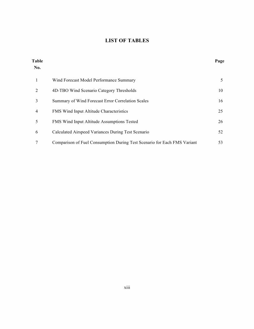
LIST OF TABLES

Table Page No.

1 Wind Forecast Model Performance Summary 5

2 4D-TBO Wind Scenario Category Thresholds 10

3 Summary of Wind Forecast Error Correlation Scales 16

4 FMS Wind Input Altitude Characteristics 25

5 FMS Wind Input Altitude Assumptions Tested 26

6 Calculated Airspeed Variances During Test Scenario 52

7 Comparison of Fuel Consumption During Test Scenario for Each FMS Variant 53


1

1. INTRODUCTION

1.1 MOTIVATION FOR RESEARCH

Accurate wind information is of fundamental importance to some of the critical future air traffic concepts envisioned under the FAA’s Next Generation Air Transportation System (NextGen) and EUROCONTROL’s Single European Sky (SESAR) initiatives. Concepts involving time elements, such as Four-Dimensional Trajectory Based Operations (4D-TBO) and Interval Management (IM), are especially sensitive to wind information accuracy. Under 4D-TBO, an aircraft is assigned an appropriate Required Time of Arrival (RTA) at a meter fix some distance in the future, which they are expected to meet to some time tolerance. In an IM procedure, a leader/follower pair of aircraft is identified and a relative time separation target between the pair is defined that needs to be accomplished by a specific point. The trajectories of the two aircraft are managed in an attempt to meet the specified time target between them by this point. Errors in wind information used by ground or aircraft systems in either procedure can severely degrade the ability of these concepts to perform as intended.

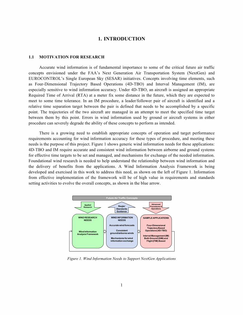
There is a growing need to establish appropriate concepts of operation and target performance requirements accounting for wind information accuracy for these types of procedure, and meeting these needs is the purpose of this project. Figure 1 shows generic wind information needs for these applications: 4D-TBO and IM require accurate and consistent wind information between airborne and ground systems for effective time targets to be set and managed, and mechanisms for exchange of the needed information. Foundational wind research is needed to help understand the relationship between wind information and the delivery of benefits from the applications. A Wind Information Analysis Framework is being developed and exercised in this work to address this need, as shown on the left of Figure 1. Information from effective implementation of the framework will be of high value in requirements and standards setting activities to evolve the overall concepts, as shown in the blue arrow.

Figure 1. Wind Information Needs to Support NextGen Applications

SAMPLE APPLICATIONS

Four-Dimensional Trajectory Based

Operations (4D-TBO)

Interval Management (IM)Both Ground (GIM) and

Flight (FIM) Based

WIND RESEARCH NEEDS

Wind Information Analysis Framework

Future Air Traffic Concepts

WIND INFORMATION NEEDS

Accurate wind forecasts

Consistentground/airborne winds

Mechanisms for wind information exchange

Applied Research

Advanced Procedures &

OperationsReqts/

Standards Guidance

2

1.2 WIND INFORMATION ANALYSIS FRAMEWORK

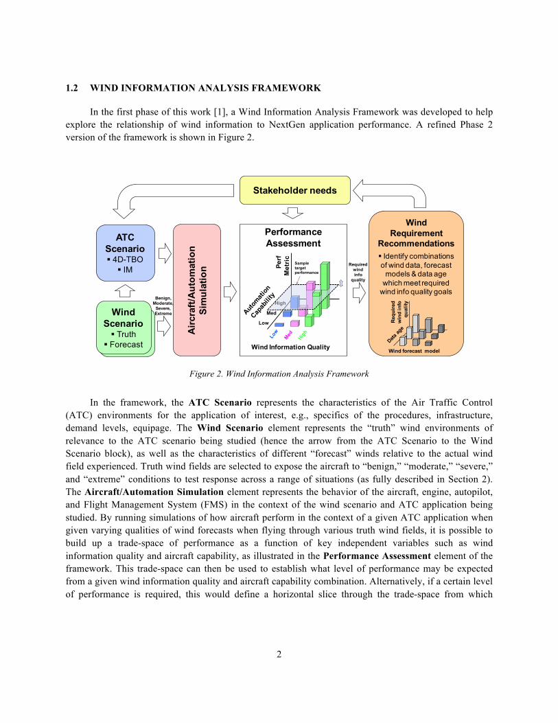
In the first phase of this work [1], a Wind Information Analysis Framework was developed to help explore the relationship of wind information to NextGen application performance. A refined Phase 2 version of the framework is shown in Figure 2.

Figure 2. Wind Information Analysis Framework

In the framework, the ATC Scenario represents the characteristics of the Air Traffic Control (ATC) environments for the application of interest, e.g., specifics of the procedures, infrastructure, demand levels, equipage. The Wind Scenario element represents the “truth” wind environments of relevance to the ATC scenario being studied (hence the arrow from the ATC Scenario to the Wind Scenario block), as well as the characteristics of different “forecast” winds relative to the actual wind field experienced. Truth wind fields are selected to expose the aircraft to “benign,” “moderate,” “severe,” and “extreme” conditions to test response across a range of situations (as fully described in Section 2). The Aircraft/Automation Simulation element represents the behavior of the aircraft, engine, autopilot, and Flight Management System (FMS) in the context of the wind scenario and ATC application being studied. By running simulations of how aircraft perform in the context of a given ATC application when given varying qualities of wind forecasts when flying through various truth wind fields, it is possible to build up a trade-space of performance as a function of key independent variables such as wind information quality and aircraft capability, as illustrated in the Performance Assessment element of the framework. This trade-space can then be used to establish what level of performance may be expected from a given wind information quality and aircraft capability combination. Alternatively, if a certain level of performance is required, this would define a horizontal slice through the trade-space from which

Performance Assessment

Wind Scenario§ Truth

§ Forecast

Airc

raft/

Aut

omat

ion

Sim

ulat

ion

Stakeholder needs

ATCScenario§ 4D-TBO

§ IM

WindRequirement

Recommendations§ Identify combinations of wind data, forecast

models & data age which meet required

wind info quality goals

Perf

Met

ric

Wind Information Quality

Low

Med

High

Sampletargetperformance

Requ

ired

win

d in

foqu

ality

Wind forecast model

Benign,Moderate,

Severe,Extreme

Requiredwindinfo

quality

3

combinations of wind information quality and aircraft capability that exceed that standard can be identified. The Wind Requirement Recommendations element identifies which combinations of wind data content, from which specific operational wind forecast models and with what data age meet the wind information quality level identified from the previous element that achieve the target procedure performance. Finally, the Stakeholder Needs element represent the key role of stakeholders in determining appropriate choices in the other framework elements, e.g., in terms of which scenarios and performance metrics are of value to them to support the creation of guidance or requirements documents or to inform appropriate Concepts of Operation.

The framework is designed to be scalable with respect to scope and fidelity of its individual elements, as well as flexible with respect to the specific ATC application being studied. In Phase 1 of this project, the utility of this framework was initially demonstrated using simplified version of the framework elements applied to a simple 4D-TBO scenario. This demonstrated significant insights that could be generated from its use, as discussed in [1, 2, 3]. Phase 2 has further refined the 4D-TBO analysis and expanded into IM applications.

1.3 PHASE 2 FOCUS AREAS

Phase 2 of the work reported here has built upon the Phase 1 foundation by using refined and expanded applications of the Wind Information Analysis Framework. These activities are reported in this document as follows:

• Section 2: documents the refined wind information metrics and wind scenario selection process applicable to a broader range of NextGen applications, with particular focus on 4D-TBO and IM.

• Section 3: presents the expanded and refined studies of 4D-TBO applications with current FMSs (with MITRE collaboration) to identify more accurate trade-spaces using operational FMS capabilities with higher-fidelity aircraft models.

• Section 4: discusses the expansion of the 4D-TBO study using incremental enhancements possible in future FMSs (with Honeywell collaboration), specifically in the area of wind blending algorithms to quantify performance improvement potential from near-term avionics refinements.

• Section 5: demonstrates the adaptability of the Wind Information Analysis Framework by using

it to identify initial wind information needs for IM applications.

• Section 6: Summarizes the key findings and recommendations from this work to date.

4

1.4 REFERENCES

[1] Reynolds, T.G., Y. Glina, S.W. Troxel, and M.D. McPartland, “Wind Information Requirements for NextGen Applications Phase 1: 4D-Trajectory Based Operations (4D-TBO),” Project Report ATC-399, MIT Lincoln Laboratory, 2013.

[2] Glina, Y., T.G. Reynolds, S. Troxel, and M. McPartland, “Wind Information Requirements to Support Four Dimensional Trajectory-Based Operations,” 12th AIAA Aviation Technology, Integration, and Operations Conference, Indianapolis, IN, AIAA 2012-5702, 2012.

[3] Reynolds, T.G., S. Troxel, Y. Glina, and M. McPartland, “Establishing Wind Information Needs for Four Dimensional Trajectory-Based Operations,” 1st International Conference on Interdisciplinary Science for Innovative Air Traffic Management, Daytona Beach, FL, 2012.

5

2. REFINING WIND INFORMATION METRICS AND ANALYSIS SCENARIOS

2.1 INTRODUCTION

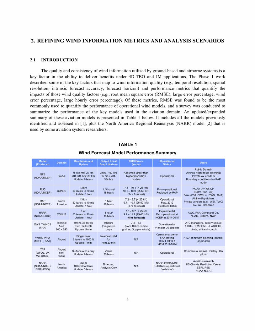
The quality and consistency of wind information utilized by ground-based and airborne systems is a key factor in the ability to deliver benefits under 4D-TBO and IM applications. The Phase 1 work described some of the key factors that map to wind information quality (e.g., temporal resolution, spatial resolution, intrinsic forecast accuracy, forecast horizon) and performance metrics that quantify the impacts of those wind quality factors (e.g., root mean square error (RMSE), large error percentage, wind error percentage, large hourly error percentage). Of these metrics, RMSE was found to be the most commonly used to quantify the performance of operational wind models, and a survey was conducted to summarize the performance of the key models used in the aviation domain. An updated/expanded summary of these aviation models is presented in Table 1 below. It includes all the models previously identified and assessed in [1], plus the North America Regional Reanalysis (NARR) model [2] that is used by some aviation system researchers.

TABLE 1

Wind Forecast Model Performance Summary

Model(Producer) Domain Resolution and

UpdateOutput Fcast

Step / HorizonRMS Errors

(knots)Operational

Status Users

GFS(NOAA/NCEP) Global

0-192 hrs: 25 km204-384 hrs: 80 km

Update: 6 hours

3 hrs / 192 hrs12 hrs / 204-

384 hrs

Assumed larger than higher resolution

modelsOperational

Public DomainAirlines (f light route planning)

Private wx vendorsBoundary conditions for RAP

model

RUC(NOAA/NCEP) CONUS

13 km50 levels to 50 mb

Update: 1 hour

1, 3 hours/ 18 hours

7.6 – 10.1 (< 25 kf t)10.1 – 10.9 (25-50 kf t)

(3-hr forecast)

Prior operationalReplaced by RAP

NOAA (Av.Wx.Ctr,Storm Pred. Ctr)

FAA (ATM, CWSUs, ITWS, TMA)Airline dispatchers

Private vendors (e.g., WSI, TWC)Av. Wx. Research

RAP(NOAA/NCEP)

NorthAmerica


Update: 1 hour

1 hour18 hours

7.2 – 9.7 (< 25 kf t)9.7 – 10.7 (25-50 kf t)

(3-hr forecast)

OperationalMay, 2012

(Replaces RUC)

HRRR(NOAA/ESRL) CONUS


Update: 1 hour

1 hour/15 hours

7.8 – 9.7 (< 25 kf t9.7 – 11.7 (25-45 kf t)

(6-hr forecast)

ExperimentalEst. operational atNCEP in 2014-2015

AWC, FAA Command Ctr, NCAR, CoSPA, NWP

ITWS TWINDS(FAA)

TerminalArea

240 x 240

10 km, 36 levels2 km, 24 levelsUpdate: 5 min

0 hours(diagnostic

only)

7.4 – 8.7(f rom 10-km coarse

grid, no Doppler winds)

Operational at44 major US airports

ATC managers, supervisors at ATCTs, TRACONs, & ARTCCs,

pilots, airline dispatch

WTMD WFA(MIT LL, FAA) Airport

Single point6 levels to 1000 f t

Update: 1 min

Nowcast valid for

next 20 minN/A

Operational demoFAA testing

at IAH, SFO & MEM 2012-2014

ATC for runway planning (parallel approach)

TAF(WFOs, UK Met Off ice)

Airport5 mi

radius

Surface winds onlyUpdate: 6 hours

Varies30 hours N/A Operational Commercial airlines, military, GA

pilots

NARR(NOAA/NCEP/ ESRL/PSD)

North America

32km40 level to 30mbUpdate: 3 hours

Time zero Analysis Only N/A

NARR (1979-2003)R-CDAS (operational

“real-time”)

Aviation researchUS Climate Prediction Center

ESRL-PSDNOAA-NCDC

6

As NextGen application focus areas expand, it has become necessary to develop a generic approach to identifying appropriate wind metrics, truth and forecast wind scenarios, and ATC trajectories for use in the Wind Information Analysis Framework. The following sections describe a general process for refining the identification of appropriate wind information metrics, and how this process can be used to select the truth and forecast wind scenarios used in the analysis framework.

2.2 WIND INFORMATION METRIC AND SCENARIO SELECTION PROCESS

The choice of wind metric is critical to the analysis of wind needs for NextGen applications because they are the mechanism by which the notional “low,” “medium,” and “high” wind information quality shown in Figure 2 is quantified for the Performance Assessment trade-space. In order for these trade-spaces to be useful, the chosen metrics need to discriminate wind environments that result in operationally realistic ranges of aircraft performance and wind forecasts for a given application.

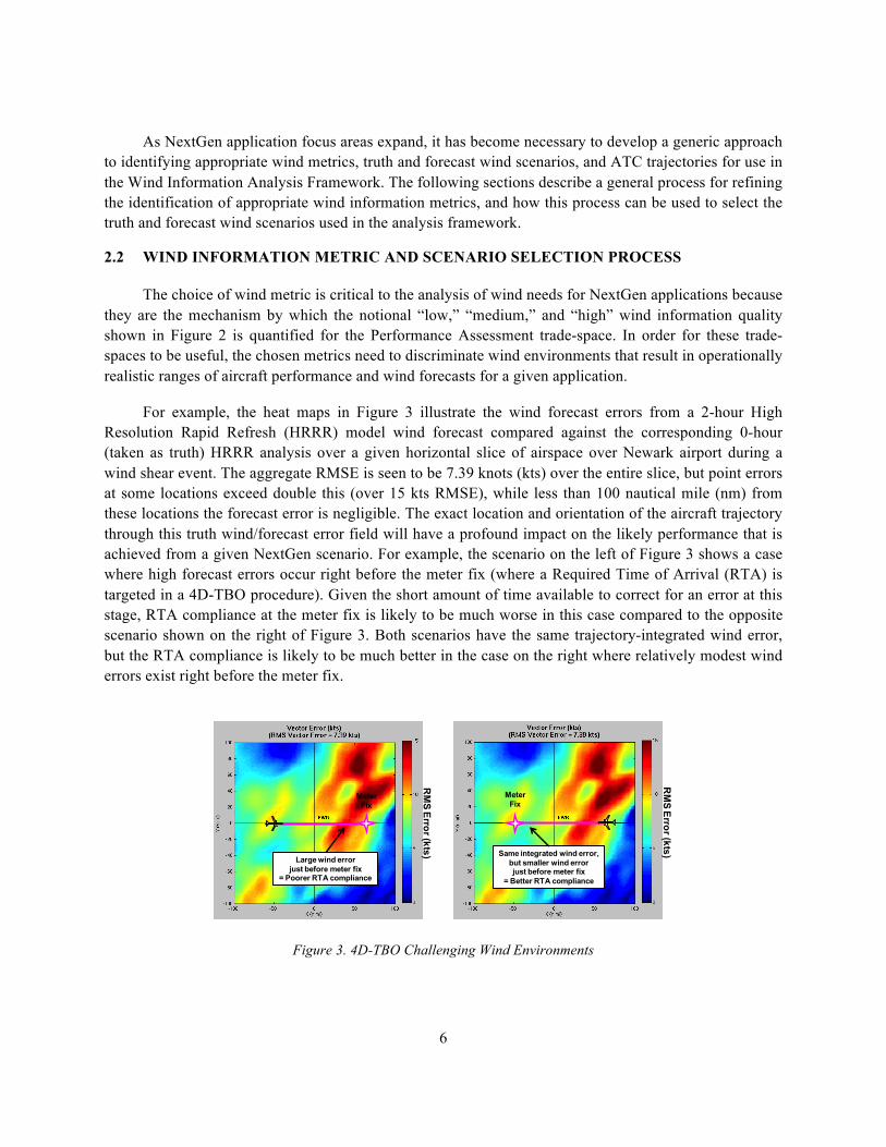
For example, the heat maps in Figure 3 illustrate the wind forecast errors from a 2-hour High Resolution Rapid Refresh (HRRR) model wind forecast compared against the corresponding 0-hour (taken as truth) HRRR analysis over a given horizontal slice of airspace over Newark airport during a wind shear event. The aggregate RMSE is seen to be 7.39 knots (kts) over the entire slice, but point errors at some locations exceed double this (over 15 kts RMSE), while less than 100 nautical mile (nm) from these locations the forecast error is negligible. The exact location and orientation of the aircraft trajectory through this truth wind/forecast error field will have a profound impact on the likely performance that is achieved from a given NextGen scenario. For example, the scenario on the left of Figure 3 shows a case where high forecast errors occur right before the meter fix (where a Required Time of Arrival (RTA) is targeted in a 4D-TBO procedure). Given the short amount of time available to correct for an error at this stage, RTA compliance at the meter fix is likely to be much worse in this case compared to the opposite scenario shown on the right of Figure 3. Both scenarios have the same trajectory-integrated wind error, but the RTA compliance is likely to be much better in the case on the right where relatively modest wind errors exist right before the meter fix.

Figure 3. 4D-TBO Challenging Wind Environments

RM

S Error (kts)

RM

S Error (kts)

Large wind errorjust before meter fix

= Poorer RTA compliance

Same integrated wind error,but smaller wind errorjust before meter fix

= Better RTA compliance

MeterFix

MeterFix

7

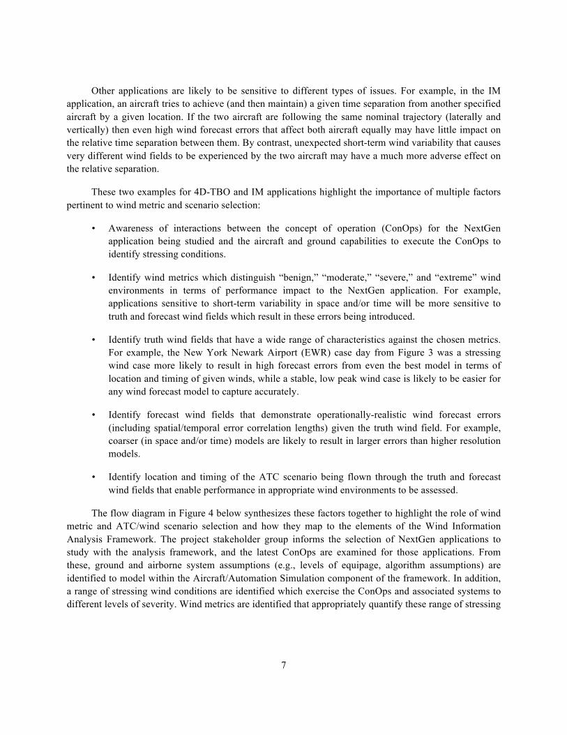
Other applications are likely to be sensitive to different types of issues. For example, in the IM application, an aircraft tries to achieve (and then maintain) a given time separation from another specified aircraft by a given location. If the two aircraft are following the same nominal trajectory (laterally and vertically) then even high wind forecast errors that affect both aircraft equally may have little impact on the relative time separation between them. By contrast, unexpected short-term wind variability that causes very different wind fields to be experienced by the two aircraft may have a much more adverse effect on the relative separation.

These two examples for 4D-TBO and IM applications highlight the importance of multiple factors pertinent to wind metric and scenario selection:

• Awareness of interactions between the concept of operation (ConOps) for the NextGen application being studied and the aircraft and ground capabilities to execute the ConOps to identify stressing conditions.

• Identify wind metrics which distinguish “benign,” “moderate,” “severe,” and “extreme” wind environments in terms of performance impact to the NextGen application. For example, applications sensitive to short-term variability in space and/or time will be more sensitive to truth and forecast wind fields which result in these errors being introduced.

• Identify truth wind fields that have a wide range of characteristics against the chosen metrics. For example, the New York Newark Airport (EWR) case day from Figure 3 was a stressing wind case more likely to result in high forecast errors from even the best model in terms of location and timing of given winds, while a stable, low peak wind case is likely to be easier for any wind forecast model to capture accurately.

• Identify forecast wind fields that demonstrate operationally-realistic wind forecast errors (including spatial/temporal error correlation lengths) given the truth wind field. For example, coarser (in space and/or time) models are likely to result in larger errors than higher resolution models.

• Identify location and timing of the ATC scenario being flown through the truth and forecast wind fields that enable performance in appropriate wind environments to be assessed.

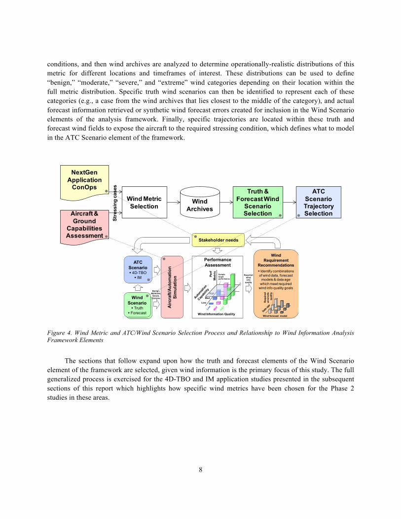
The flow diagram in Figure 4 below synthesizes these factors together to highlight the role of wind metric and ATC/wind scenario selection and how they map to the elements of the Wind Information Analysis Framework. The project stakeholder group informs the selection of NextGen applications to study with the analysis framework, and the latest ConOps are examined for those applications. From these, ground and airborne system assumptions (e.g., levels of equipage, algorithm assumptions) are identified to model within the Aircraft/Automation Simulation component of the framework. In addition, a range of stressing wind conditions are identified which exercise the ConOps and associated systems to different levels of severity. Wind metrics are identified that appropriately quantify these range of stressing

8

conditions, and then wind archives are analyzed to determine operationally-realistic distributions of this metric for different locations and timeframes of interest. These distributions can be used to define “benign,” “moderate,” “severe,” and “extreme” wind categories depending on their location within the full metric distribution. Specific truth wind scenarios can then be identified to represent each of these categories (e.g., a case from the wind archives that lies closest to the middle of the category), and actual forecast information retrieved or synthetic wind forecast errors created for inclusion in the Wind Scenario elements of the analysis framework. Finally, specific trajectories are located within these truth and forecast wind fields to expose the aircraft to the required stressing condition, which defines what to model in the ATC Scenario element of the framework.

Figure 4. Wind Metric and ATC/Wind Scenario Selection Process and Relationship to Wind Information Analysis Framework Elements

The sections that follow expand upon how the truth and forecast elements of the Wind Scenario element of the framework are selected, given wind information is the primary focus of this study. The full generalized process is exercised for the 4D-TBO and IM application studies presented in the subsequent sections of this report which highlights how specific wind metrics have been chosen for the Phase 2 studies in these areas.


Wind Scenario§ Truth

§ Forecast

Airc

raft/

Aut

omat

ion

Sim

ulat

ion

Stakeholder needs

ATCScenario§ 4D-TBO

§ IM

WindRequirement

Recommendations§ Identify combinations of wind data, forecast

models & data age which meet required

wind info quality goals

Perf

Met

ric

Wind Information Quality

Low

Med

High

Sampletargetperformance

Requ

ired

win

d in

foqu

ality

Wind forecast model

Benign,Moderate,

Severe,Extreme

Requiredwindinfo

quality

NextGenApplication

ConOps

Aircraft & Ground

Capabilities Assessment

Wind Metric Selection

Truth & Forecast Wind

Scenario Selection

Wind Archives

ATC ScenarioTrajectory Selection

Stre

ssin

g ca

ses

9

2.3 TRUTH WIND SCENARIO SELECTION APPROACHES

Once the appropriate wind information metrics have been identified for the NextGen application of interest, historical numerical weather prediction model data (such as Rapid Refresh (RAP) or HRRR) can be collected and processed to identify truth wind fields representative of defined statistical value ranges for the chosen metric (e.g., benign, moderate, severe, extreme). Defining meaningful and representative classification thresholds involves first determining the spatio-temporal distributions of that wind metric. Note that the severity or intensity classification of a selected scenario with regard to the chosen metric arises from the combined effects of the wind environment and the geometry of the trajectory through that environment, so both of these elements need to be taken into account when constructing the scenario. Two approaches to truth wind scenario selection have been explored in Phase 2 of this work:

1. Volumetric-based 2. Trajectory-based

The following subsections illustrate the two selection approaches using examples from the Phase 2 studies. Variants of these approaches may be more appropriate for other studies which may be explored further in Phase 3.

2.3.1 Volumetric-Based Wind Scenario Selection Approach

This approach defines volumes of airspace within which wind parameters observed in the field can be analyzed. The range of observed behaviors in that volume can be used as the basis for appropriate statistical categories reflecting different magnitudes of the chosen wind metric(s). The midpoints of these categories can be used to identify case days that are statistically-representative of the category as a whole, or the basis for synthetic wind fields with appropriate characteristics. This approach is appropriate for classifying the general wind environment independent of any specific trajectory.

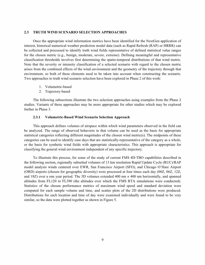
To illustrate this process, for some of the study of current FMS 4D-TBO capabilities described in the following section, regionally subsetted volumes of 13 km resolution Rapid Update Cycle (RUC)/RAP model analysis winds centered over EWR, San Francisco Airport (SFO), and Chicago O’Hare Airport (ORD) airports (chosen for geographic diversity) were processed at four times each day (00Z, 06Z, 12Z, and 18Z) over a one year period. The 3D volumes extended 400 nm × 400 nm horizontally, and spanned altitudes from FL120 to FL390 (the altitudes over which the FMS RTA simulations were conducted). Statistics of the chosen performance metrics of maximum wind speed and standard deviation were computed for each sample volume and time, and scatter plots of the 2D distributions were produced. Distributions for each location and time of day were examined individually and were found to be very similar, so the data were plotted together as shown in Figure 5.

10

Figure 5. Partitioning of Wind Speed and Standard Deviation for 4D-TBO Wind Scenario Classification

From the combined distribution, a 2D partitioning (max wind speed, standard deviation) was constructed such that 25% of the points fell into the “benign” category, 50% in the “moderate” category, and 25% in the “severe” category. The upper limit of observed behaviors can also be used to define an “extreme” category to identify the most stressing (but still operationally realistic) case(s). Table 2 summarizes the category thresholds based on this partitioning of the distribution in Figure 5. Once the distribution has been partitioned, specific wind cases having statistics corresponding to the midpoints of the categories can be selected as candidates that make up the test wind scenarios.

TABLE 2

4D-TBO Wind Scenario Category Thresholds

Category Max Speed (knots) Std Dev (knots) Benign <70 <20

Moderate 75–115 20–30 Severe 115+ 30+

2.3.2 Trajectory-Based Wind Scenario Selection Approach

One of the practical challenges encountered when using the volumetric wind scenario classification approach discussed above, is that the metrics computed over the volume, while generally indicative of the

11

wind environment and useful for identifying candidate cases, do not necessarily produce the desired characteristic of the wind metric that a specific trajectory would yield when flown through those winds. Indeed, the statistics can result from points at opposite corners of the study volume that are many hundreds of miles apart. If the procedure is to be flown along established fixed routes (such as existing Standard Terminal Arrival Routes (STARs) into a given airport), one might need to test several candidate wind fields together with the trajectory before finding the optimal combination of winds and trajectory. If synthetic routes (e.g., straight line) are being used, an iterative process of strategic re-positioning and orientation of the synthetic trajectory on the candidate wind field can be employed to arrive at a final wind/trajectory combination that meets the intended criteria.

In Phase 2, we found that computing the distributions of chosen wind metric values from winds sampled along the specific trajectories to be flown (synthetic or real) more directly yielded appropriate test combinations of winds and trajectory to produce the desired metric value. This route-based scenario selection approach has been developed and used to classify and identify potential IM scenarios in the work presented in Section 5. For example, a key wind metric for IM is high spatio-temporal variability of the winds whereby the ownship and traffic-to-follow may experience significantly different and/or rapidly changing headwinds.

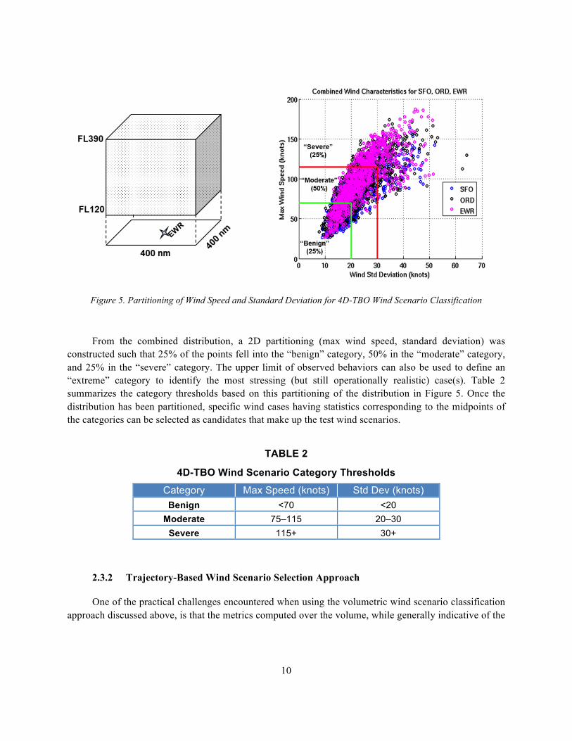
To illustrate the process, the coordinates for the Phoenix Airport Approach Procedure (EAGUL5) STAR trajectory into Phoenix International Airport (PHX) (Figure 6) were used to sample RAP model analysis winds at 1 nm intervals along that route over a one year period at four times each day (00Z, 06Z, 12Z, 18Z).

Figure 6. Lateral (left) and Vertical Profile (right) Depiction of the EAGUL5 Approach to PHX Airport

12

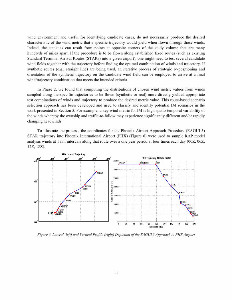
The standard deviations of the headwinds encountered for the entire trajectory were aggregated for the one-year period, resulting in the distribution shown in the top half of Figure 7. The bottom half of Figure 7 presents the cumulative probability of headwind standard deviation. The cumulative probability distribution was then thresholded to partition the distribution at the 25th and 75th percentiles to produce three category ranges corresponding to benign, moderate, and severe headwind variability for the route (green and red lines demarcate the partitioning of the distribution for the three categories). Standard deviation values corresponding to the midpoints of the categories are indicated on the cumulative probability curve in the lower half of Figure 7.

Figure 7. Headwind Variability Distribution and Classification Thresholds for EAGUL5 Approach to PHX

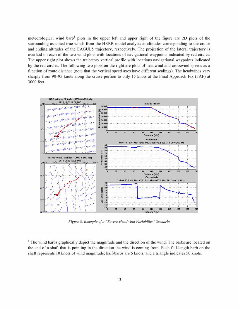
To illustrate how these results can be used to identify case days representative of one category, Figure 8 shows an example of a wind/trajectory scenario having a headwind variability corresponding to the midpoint of the “severe” variability category, with a headwind standard deviation of 24.3 knots. The

13

meteorological wind barb1 plots in the upper left and upper right of the figure are 2D plots of the surrounding assumed true winds from the HRRR model analysis at altitudes corresponding to the cruise and ending altitudes of the EAGUL5 trajectory, respectively. The projection of the lateral trajectory is overlaid on each of the two wind plots with locations of navigational waypoints indicated by red circles. The upper right plot shows the trajectory vertical profile with locations navigational waypoints indicated by the red circles. The following two plots on the right are plots of headwind and crosswind speeds as a function of route distance (note that the vertical speed axes have different scalings). The headwinds vary sharply from 90–95 knots along the cruise portion to only 15 knots at the Final Approach Fix (FAF) at 3000 feet.

Figure 8. Example of a “Severe Headwind Variability” Scenario

1 The wind barbs graphically depict the magnitude and the direction of the wind. The barbs are located on the end of a shaft that is pointing in the direction the wind is coming from. Each full-length barb on the shaft represents 10 knots of wind magnitude; half-barbs are 5 knots, and a triangle indicates 50 knots.

14

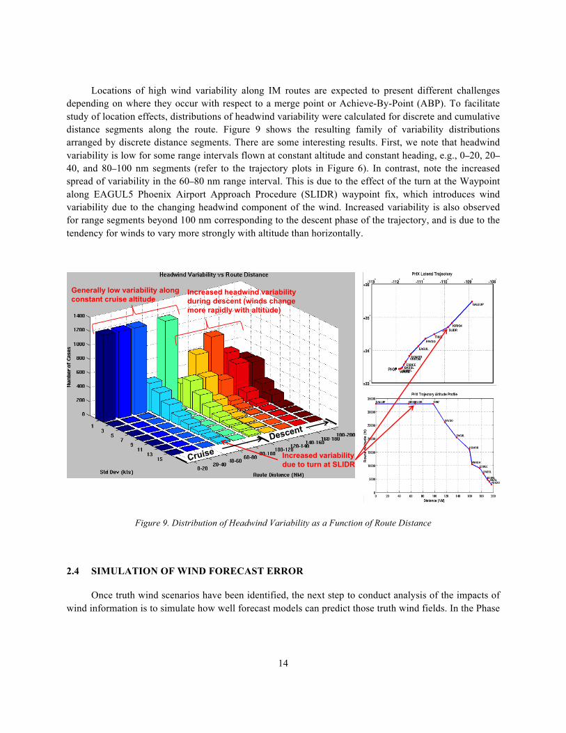
Locations of high wind variability along IM routes are expected to present different challenges depending on where they occur with respect to a merge point or Achieve-By-Point (ABP). To facilitate study of location effects, distributions of headwind variability were calculated for discrete and cumulative distance segments along the route. Figure 9 shows the resulting family of variability distributions arranged by discrete distance segments. There are some interesting results. First, we note that headwind variability is low for some range intervals flown at constant altitude and constant heading, e.g., 0–20, 20–40, and 80–100 nm segments (refer to the trajectory plots in Figure 6). In contrast, note the increased spread of variability in the 60–80 nm range interval. This is due to the effect of the turn at the Waypoint along EAGUL5 Phoenix Airport Approach Procedure (SLIDR) waypoint fix, which introduces wind variability due to the changing headwind component of the wind. Increased variability is also observed for range segments beyond 100 nm corresponding to the descent phase of the trajectory, and is due to the tendency for winds to vary more strongly with altitude than horizontally.

Figure 9. Distribution of Headwind Variability as a Function of Route Distance

2.4 SIMULATION OF WIND FORECAST ERROR

Once truth wind scenarios have been identified, the next step to conduct analysis of the impacts of wind information is to simulate how well forecast models can predict those truth wind fields. In the Phase

Increased variabilitydue to turn at SLIDR

Increased headwind variability during descent (winds change more rapidly with altitude)

Generally low variability along constant cruise altitude

15

1 work, and as summarized in Section 2.1, characteristics and quality factors of current wind forecast models used in the aviation domain and their typical performance have been identified. RMS errors in the range of 0–12.5 kts are observed on aggregate, but due to the averaging property, point errors can be much larger than this. Figure 3 illustrates a case where point errors are up to double the average value, suggesting an error range of 0–25 kts RMSE as being operationally realistic, and that wind forecast error range was used in the Phase 1 analysis.

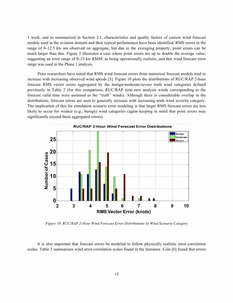
Prior researchers have noted that RMS wind forecast errors from numerical forecast models tend to increase with increasing observed wind speeds [3]. Figure 10 plots the distributions of RUC/RAP 2-hour forecast RMS vector errors aggregated by the benign/moderate/severe truth wind categories defined previously in Table 2 (for this comparison, RUC/RAP time-zero analysis winds corresponding to the forecast valid time were assumed as the “truth” winds). Although there is considerable overlap in the distributions, forecast errors are seen to generally increase with increasing truth wind severity category. The implication of this for simulation scenario error modeling is that larger RMS forecast errors are less likely to occur for weaker (e.g., benign) wind categories (again keeping in mind that point errors may significantly exceed these aggregated errors).

Figure 10. RUC/RAP 2-Hour Wind Forecast Error Distributions by Wind Scenario Category

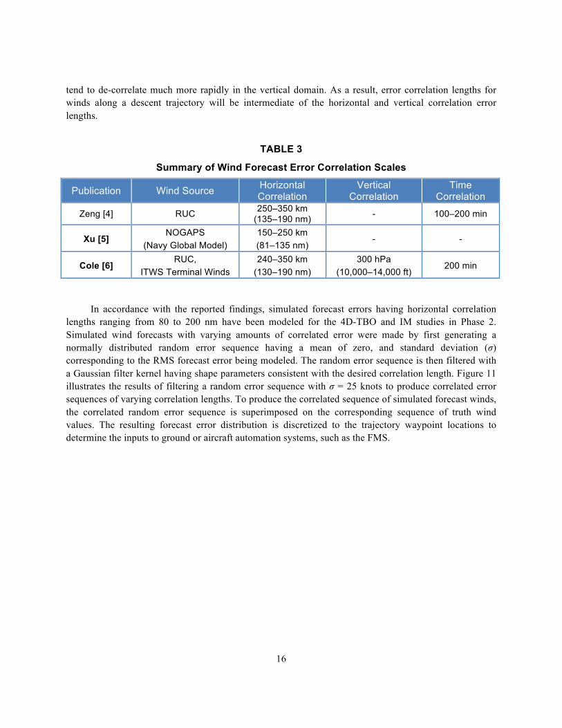
It is also important that forecast errors be modeled to follow physically realistic error correlation scales. Table 3 summarizes wind error correlation scales found in the literature. Cole [6] found that errors

RMS Vector Error (knots)2 3 4 5 6 7 8 9 10

25

20

15

10

5

0

Num

ber o

f Cas

es

16

tend to de-correlate much more rapidly in the vertical domain. As a result, error correlation lengths for winds along a descent trajectory will be intermediate of the horizontal and vertical correlation error lengths.

TABLE 3

Summary of Wind Forecast Error Correlation Scales

Publication Wind Source Horizontal Correlation

Vertical Correlation

Time Correlation

Zeng [4] RUC 250–350 km (135–190 nm) - 100–200 min

Xu [5] NOGAPS

(Navy Global Model) 150–250 km (81–135 nm)

- -

Cole [6] RUC,

ITWS Terminal Winds 240–350 km

(130–190 nm) 300 hPa

(10,000–14,000 ft) 200 min

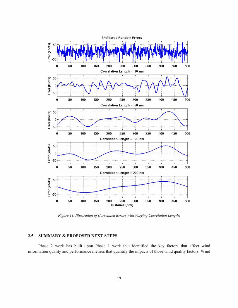
In accordance with the reported findings, simulated forecast errors having horizontal correlation lengths ranging from 80 to 200 nm have been modeled for the 4D-TBO and IM studies in Phase 2. Simulated wind forecasts with varying amounts of correlated error were made by first generating a normally distributed random error sequence having a mean of zero, and standard deviation (σ) corresponding to the RMS forecast error being modeled. The random error sequence is then filtered with a Gaussian filter kernel having shape parameters consistent with the desired correlation length. Figure 11 illustrates the results of filtering a random error sequence with σ = 25 knots to produce correlated error sequences of varying correlation lengths. To produce the correlated sequence of simulated forecast winds, the correlated random error sequence is superimposed on the corresponding sequence of truth wind values. The resulting forecast error distribution is discretized to the trajectory waypoint locations to determine the inputs to ground or aircraft automation systems, such as the FMS.

17

Figure 11. Illustration of Correlated Errors with Varying Correlation Lengths

2.5 SUMMARY & PROPOSED NEXT STEPS

Phase 2 work has built upon Phase 1 work that identified the key factors that affect wind information quality and performance metrics that quantify the impacts of those wind quality factors. Wind

18

information quality is dictated by a combination of wind data quality factors. For NextGen applications such as 4D-TBO and IM, the following quality factors were identified as potentially significant: timeliness (update rate, latency), spatial/temporal resolution, and intrinsic forecast accuracy, all of which combine to give a particular model its forecast skill. Location, extent, and duration of forecast errors are additional important qualities of winds and wind forecasts. Prolonged exposure to correlated forecast errors along a trajectory can lead to significant Estimated Time of Arrival (ETA) errors that can reduce the likelihood of achieving a given procedure (such as the ability to meet an RTA).

Comparisons of operational wind forecast models have been updated given latest information and expanded to cover more models used in the aviation community. A general process model has been created that shows the importance of understanding the Concept of Operation, aircraft and ground capabilities in the selection of appropriate wind metrics of interest for a given NextGen application, which can then be used to identify appropriate truth and forecast wind scenarios. Two truth wind scenario selection approaches (volumetric and trajectory-based) have been described and illustrated. Simulating realistic wind forecast errors has also been described using techniques that respect the magnitude of RMS error and spatial/temporal correlation characteristics seen in the operational wind forecast models used in the aviation domain.

Moving forward, Phase 3 work will examine refinements to the trajectory-based wind scenario selection approach, which not only account for the aggregate wind characteristics along a given trajectory, but also where they occur along the trajectory. Referring back to Figure 3, such an approach could distinguish between wind variability and forecast error location relative to the meter fix location and therefore allow an assessment of this potentially important performance driver.

2.6 REFERENCES


[2] Mesinger, F., G. Dimego, E. Kalnay, K. Mitchell, P.C. Shafran, W. Ebisuzaki, D. Jović, J. Woollen, E. Rogers, E.H. Berbery, M.B. Ek, Y. Fan, R. Grumbine, W. Higgins, H. Li, Y. Lin, G. Manikin, D. Parrish, and W. Shi, “North American Regional Reanalysis,” Bulletin of the American Meteorological Society, DOI:10.1175/BAMS-87-3-343, March 2006.

[3] Schwartz, B.E., S.G. Benjamin: Accuracy of RUC-1 and RUC-2 Wind and Aircraft Trajectory Forecasts as Determined from ACARS Observations, Weather and Forecasting, 15 June 2000.

[4] Zheng, Q. Maggie, J.Z. Zhao: Modeling Wind Uncertainties for Stochastic Trajectory Synthesis, 11th AIAA Aviation Technology, Integration, and Operations (ATIO) Conference, Sep 2011.

19

[5] Xu, Qin, Li Wei, 2001: Estimation of Three-Dimensional Error Covariances. Part II: Analysis of Wind Innovation Vectors. Mon. Wea. Rev., 129, 2939–2954.

[6] Cole, R.E., Green, S.M., and Jardin, M.R., Improving RUC-1 Wind Estimates by Incorporating Near-Real-Time Aircraft Reports, Weather and Forecasting, Volume 15, Number 4, pp. 447–460, August 2000.


21

3. WIND INFORMATION ANALYSIS FOR 4D-TBO APPLICATIONS WITH CURRENT FMS

3.1 INTRODUCTION

Phase 1 of this work demonstrated the use of the Wind Information Analysis Framework using a simplified version of the framework elements (e.g., MATLAB-based engineering versions of the FMS capabilities and simplified aircraft performance models) applied to a simple 4D-TBO application. This acted as an effective “proof-of-concept” of the utility of the framework for developing trade-spaces relating wind information quality, aircraft capability and 4D-TBO performance from which wind requirements could be established, in principle. This section documents the refinements and extensions made during Phase 2 to identify more accurate trade-spaces using actual/re-hosted FMS capabilities and higher-fidelity aircraft models applied across a much broader range of wind and ATC scenarios compared to Phase 1.

3.2 MODELING APPROACH

The sections that follow describe the modeling approach pursued in the Phase 2 work, broken out according to the Wind Information Analysis Framework elements described in Section 1.

3.2.1 ATC Scenarios

The ATC scenarios studied all involved flight parameters informed by the 4D-TBO ConOps and prior flight trials (for example the Alaska Airlines trials into SEA), although the geographic location of the simulation runs was not tied to any one location. The ATC scenario trajectories were executed using the FMS (see Section 3.2.3) programmed with appropriate waypoints separated by 10 or 100 nm. For most of the scenarios studied, a straight line lateral path was used, although a sunset of runs also included turns during descent to expose the aircraft to more rapidly varying wind field characteristics. The vertical profiles comprised an initial level cruise segment at FL290 or FL390, followed by a descent to a meter fix at 12,000 ft where an RTA target was imposed at either 150 nm or 250 nm distance from the fix. The RTA target was set to be consistent with the middle, late, or early edges of the RTA window being estimated by the FMS box under test (see Section 3.2.3). Prior to RTA assignment, the aircraft was at a fixed cruise Mach number, but after RTA assignment, the RTA function of the FMS controlled the aircraft speed in an attempt to get to the meter fix to comply with the RTA.

3.2.2 Wind Scenarios

Wind fields from HRRR model analyses having wind speed and variability statistics corresponding to the midpoints of the classification regions described in Section 2.3.1 were coupled with strategic placements of synthetic 4D-TBO trajectories in order to achieve truth wind/trajectory scenarios representative of each category. Two wind/trajectory scenarios were constructed for the FMS 4D-TBO

22

tests conducted in Phase 2 corresponding to “Benign” and “Severe Headwind” wind cases. Additional scenarios corresponding to “Moderate,” “Severe,” and “Severe Tailwind” classifications were also identified, but these will be explored in detail in Phase 3. Following are descriptions of each of the wind/trajectory scenarios used to assess the current FMS 4D-TBO capabilities.

“Benign” Scenario

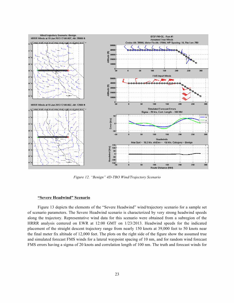
The “Benign” wind/trajectory scenario is characterized by winds having relatively low headwind speeds and low variability along the given trajectory. Representative wind data for this scenario were obtained from a subregion of the HRRR model analysis centered on SFO at 12:00 GMT on 1/19/2013. Figure 12 depicts the elements of the Benign scenario for a sample set of scenario parameters used to test the B737-700 General Electric (GE) FMS.

The meteorological wind barb plots in the upper left and upper right of the figure are 2D plots of the surrounding assumed true (HRRR analysis) winds at altitudes corresponding to the cruise and ending (meter fix) altitudes of the trajectory, respectively. The projection of the lateral trajectory is overlaid on each of the two wind plots, with the green circle indicating the starting location and the red circle indicating the ending location (a straight-line descent trajectory in this case). From the plots, the winds are generally 10–20 knots from the WNW at the selected cruise altitude of 39,000 feet, becoming generally easterly at 5–10 knots near the meter fix altitude of 12,000 feet.

The upper right plot shows the trajectory vertical profile with the assumed true winds (from the HRRR) plotted with wind barbs at each waypoint location. A lateral waypoint spacing of 10 nm and a single set of three descent altitude winds (at 10, 20, and 30 kft) permitted by the B737-700 GGE FMS are shown. The second plot in the upper right shows the simulated forecast FMS winds at each waypoint. These are the result of superimposing the spatially correlated random errors having a specified sigma and correlation length on the truth winds at each waypoint. The third plot from the top on the right shows the random simulated component wind errors (U, V) having statistics corresponding to a correlation length of 100 nm and sigma (RMS error) of 20 kts. The lowest plot on the right shows the assumed true headwinds (again based on the HRRR analysis) as a function of route distance.

23

Figure 12. “Benign” 4D-TBO Wind/Trajectory Scenario

“Severe Headwind” Scenario

Figure 13 depicts the elements of the “Severe Headwind” wind/trajectory scenario for a sample set of scenario parameters. The Severe Headwind scenario is characterized by very strong headwind speeds along the trajectory. Representative wind data for this scenario were obtained from a subregion of the HRRR analysis centered on EWR at 12:00 GMT on 1/23/2013. Headwind speeds for the indicated placement of the straight descent trajectory range from nearly 150 knots at 39,000 feet to 50 knots near the final meter fix altitude of 12,000 feet. The plots on the right side of the figure show the assumed true and simulated forecast FMS winds for a lateral waypoint spacing of 10 nm, and for random wind forecast FMS errors having a sigma of 20 knots and correlation length of 100 nm. The truth and forecast winds for

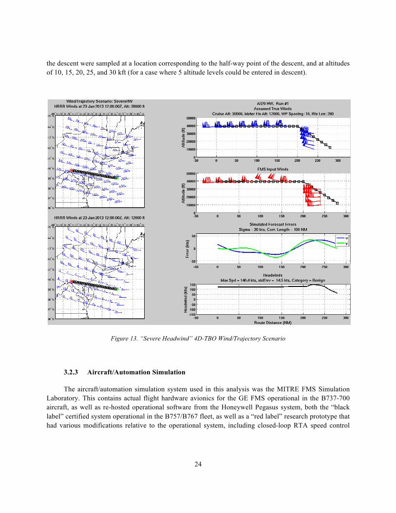
24

the descent were sampled at a location corresponding to the half-way point of the descent, and at altitudes of 10, 15, 20, 25, and 30 kft (for a case where 5 altitude levels could be entered in descent).

Figure 13. “Severe Headwind” 4D-TBO Wind/Trajectory Scenario

3.2.3 Aircraft/Automation Simulation

The aircraft/automation simulation system used in this analysis was the MITRE FMS Simulation Laboratory. This contains actual flight hardware avionics for the GE FMS operational in the B737-700 aircraft, as well as re-hosted operational software from the Honeywell Pegasus system, both the “black label” certified system operational in the B757/B767 fleet, as well as a “red label” research prototype that had various modifications relative to the operational system, including closed-loop RTA speed control

25

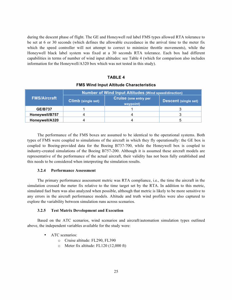
during the descent phase of flight. The GE and Honeywell red label FMS types allowed RTA tolerance to be set at 6 or 30 seconds (which defines the allowable exceedance in the arrival time to the meter fix which the speed controller will not attempt to correct to minimize throttle movements), while the Honeywell black label system was fixed at a 30 seconds RTA tolerance. Each box had different capabilities in terms of number of wind input altitudes: see Table 4 (which for comparison also includes information for the Honeywell/A320 box which was not tested in this study).

TABLE 4

FMS Wind Input Altitude Characteristics

FMS/Aircraft Number of Wind Input Altitudes (Wind speed/direction)

Climb (single set) Cruise (one entry per waypoint) Descent (single set)

GE/B737 1 1 3 Honeywell/B757 4 4 3 Honeywell/A320 4 4 5

The performance of the FMS boxes are assumed to be identical to the operational systems. Both types of FMS were coupled to simulations of the aircraft in which they fly operationally: the GE box is coupled to Boeing-provided data for the Boeing B737-700, while the Honeywell box is coupled to industry-created simulations of the Boeing B757-200. Although it is assumed these aircraft models are representative of the performance of the actual aircraft, their validity has not been fully established and this needs to be considered when interpreting the simulation results.

3.2.4 Performance Assessment

The primary performance assessment metric was RTA compliance, i.e., the time the aircraft in the simulation crossed the meter fix relative to the time target set by the RTA. In addition to this metric, simulated fuel burn was also analyzed when possible, although that metric is likely to be more sensitive to any errors in the aircraft performance models. Altitude and truth wind profiles were also captured to explore the variability between simulation runs across scenarios.

3.2.5 Test Matrix Development and Execution

Based on the ATC scenarios, wind scenarios and aircraft/automation simulation types outlined above, the independent variables available for the study were:

• ATC scenarios: o Cruise altitude: FL290, FL390 o Meter fix altitude: FL120 (12,000 ft)

26

o Waypoint spacing: 10 nm, 100 nm o RTA assignment distance: 150 nm, 250 nm o RTA location in window: Early, Middle, Late (i.e., where the assigned RTA was as

a function of the RTA window predicted by the FMS just prior to RTA assignment, with mid being the middle of the window, and early/late being 20 seconds inside the early/late edge of the window respectively)

o RTA tolerance: 6 secs, 30 secs o Lateral track: straight line positioned to achieved desired wind exposure

• Wind scenarios: o Truth wind environments: Benign, Severe headwind o Wind forecast errors (RMS vector error): Low (5 kts), Medium (12.5 kts), High (20

kts) o Wind error spatial correlation length: 50 nm

• Aircraft/automation: o Aircraft/FMS type: B737-700/GE, B757/Honeywell black label, B757/Honeywell

red label

Different combinations of these independent variables defined sets of test scenarios. A full factorial test matrix (where all combinations of independent variables are tested) was beyond the scope of the study, given all the FMS boxes were limited to run in real time. Therefore, a judicious selection of subsets of the independent variables were selected in Phase 3 to cover typical and stressing cases which would help define a range of wind information/performance trade-spaces. Similar to the MATLAB-based Phase 1 studies, a Monte Carlo simulation approach was employed. For each test scenario, up to 100 separate runs were executed in the simulation laboratory. For each run within a scenario, all variables were identical except the wind information entered into the FMS. As highlighted in Table 4, each FMS tested had different capabilities in terms of how many altitude levels wind information could be entered. Given the ATC scenarios being tested, winds were entered at the assumed altitudes shown in Table 5.

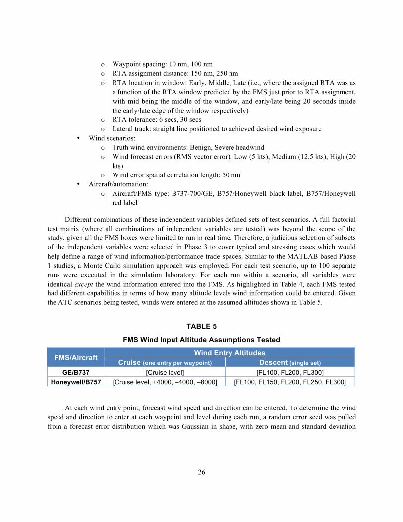
TABLE 5

FMS Wind Input Altitude Assumptions Tested

FMS/Aircraft Wind Entry Altitudes Cruise (one entry per waypoint) Descent (single set)

GE/B737 [Cruise level] [FL100, FL200, FL300] Honeywell/B757 [Cruise level, +4000, –4000, –8000] [FL100, FL150, FL200, FL250, FL300]

At each wind entry point, forecast wind speed and direction can be entered. To determine the wind speed and direction to enter at each waypoint and level during each run, a random error seed was pulled from a forecast error distribution which was Gaussian in shape, with zero mean and standard deviation

27

equal to the RMS vector error desired given the scenario being tested. As illustrated in the previous section, this error was then propagated forward in space according to the Gaussian filter kernel having shape parameters consistent with the specified correlation length. This error function was then discretized to the locations of the waypoints in the scenario being examined. The FMS wind entries at each waypoint and altitude level were determined from the simple addition of the resulting error and the truth wind at that location and altitude used in the simulation environment.

The section that follows present results for the main test scenarios studied, focusing on the results that help isolate the effects of different independent variables by keeping all others constant and observing the difference in the performance assessment metrics detailed above. Note, the results figures are identified according to the following coding scheme of independent variables:

Aircraft/Aircraft & FMS type/Truth wind scenario/Cruise altitude/Meter fix altitude/WP spacing/RTA assignment distance/Wind forecast error sigma/Error correlation length/RTA location/FMS RTA tolerance

Most of the results focus on the GE/B737 combination given the simulation laboratory had access to 12 instances of this combination, compared to only four for the Honeywell/B757 combination, such that many more scenarios could be run in parallel with the former combination.

3.3 RESULTS

3.3.1 Impact of Truth & Forecast Winds

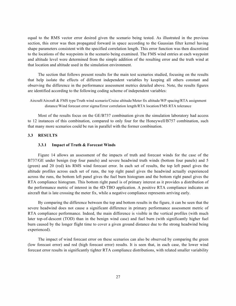
Figure 14 allows an assessment of the impacts of truth and forecast winds for the case of the B737/GE under benign (top four panels) and severe headwind truth winds (bottom four panels) and 5 (green) and 20 (red) kts RMS wind forecast error. In each set of results, the top left panel gives the altitude profiles across each set of runs, the top right panel gives the headwind actually experienced across the runs, the bottom left panel gives the fuel burn histogram and the bottom right panel gives the RTA compliance histogram. This bottom right panel is of primary interest as it provides a distribution of the performance metric of interest in the 4D-TBO application. A positive RTA compliance indicates an aircraft that is late crossing the meter fix, while a negative compliance represents arriving early.

By comparing the difference between the top and bottom results in the figure, it can be seen that the severe headwind does not cause a significant difference in primary performance assessment metric of RTA compliance performance. Indeed, the main difference is visible in the vertical profiles (with much later top-of-descent (TOD) than in the benign wind case) and fuel burn (with significantly higher fuel burn caused by the longer flight time to cover a given ground distance due to the strong headwind being experienced).

The impact of wind forecast error on these scenarios can also be observed by comparing the green (low forecast error) and red (high forecast error) results. It is seen that, in each case, the lower wind forecast error results in significantly tighter RTA compliance distributions, with related smaller variability

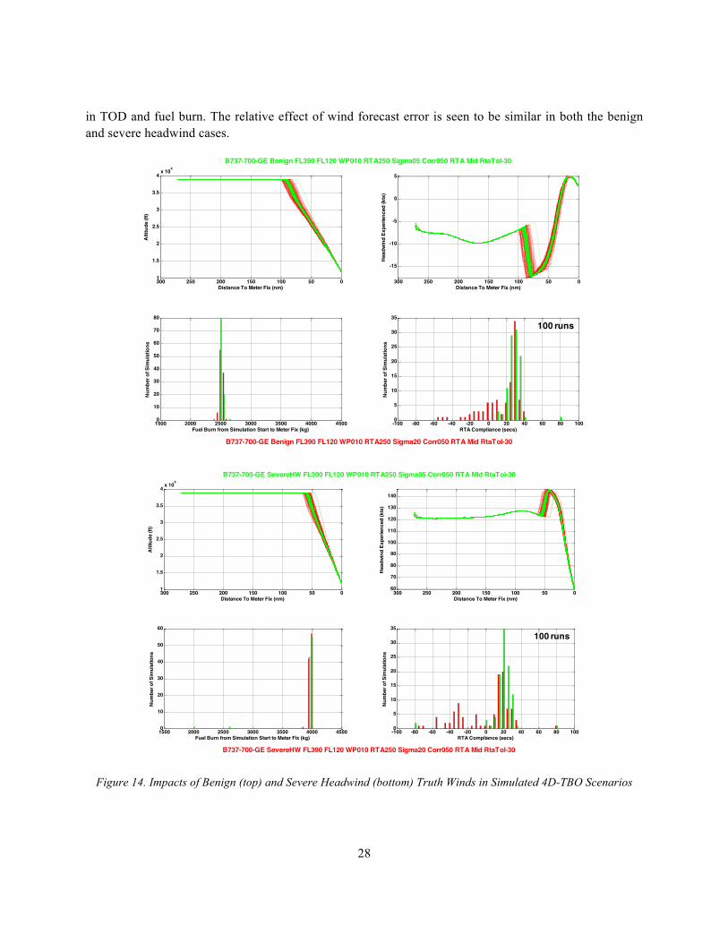
28

in TOD and fuel burn. The relative effect of wind forecast error is seen to be similar in both the benign and severe headwind cases.

Figure 14. Impacts of Benign (top) and Severe Headwind (bottom) Truth Winds in Simulated 4D-TBO Scenarios

B737-700-GE Benign FL390 FL120 WP010 RTA250 Sigma20 Corr050 RTA Mid RtaTol-30


0501001502002503001

1.5

2

2.5

3

3.5

4x 104

Distance To Meter Fix (nm)

Alti

tude

(ft)

050100150200250300

-15

-10

-5

0

5


Hea

dwin

d Ex

perie

nced

(kts

)

1500 2000 2500 3000 3500 4000 45000

10

20

30

40

50

60

70

80

Fuel Burn from Simulation Start to Meter Fix (kg)

Num

ber o

f Sim

ulat

ions

-100 -80 -60 -40 -20 0 20 40 60 80 1000

5

10

15

20

25

30

35

RTA Compliance (secs)

Num

ber o

f Sim

ulat

ions

100 runs

B737-700-GE SevereHW FL390 FL120 WP010 RTA250 Sigma05 Corr050 RTA Mid RtaTol-30


-100 -80 -60 -40 -20 0 20 40 60 80 1000

5

10

15

20

25

30

35


Num

ber o

f Sim

ulat

ions

1500 2000 2500 3000 3500 4000 45000

10

20

30

40

50

60


Num

ber o

f Sim

ulat

ions

05010015020025030060

70

80

90

100

110

120

130

140


Hea

dwin

d Ex

perie

nced

(kts

)

0501001502002503001

1.5

2

2.5

3

3.5

4x 104


Alti

tude

(ft)

100 runs

29

The positive non-zero mean in the RTA compliance distributions indicates most aircraft are late crossing the meter fix by up to 30 secs. It has been determined that this is attributable to a combination of the design of the RTA speed controller (where speed excursions of up to 15 kts can be allowable before a speed correction is made by the FMS) and aircraft model inaccuracies in the simulation environment. This combination leads to the aircraft speed being on average 7.5 kts slower than that required to meet the RTA, which manifests as a late arrival on average at the meter fix. Late bias of up to 10 seconds in the mean of the RTA compliance distributions have been observed in operational trials, indicating this is a phenomena exhibited in real world operations. However, the magnitude of some of the off-sets observed in the simulation results are greater than observed operationally. Runs in Phase 3 are correcting for this issue, but further discussions in this report focus purely on the spread of the distributions.

Another important observable characteristic in the RTA compliance results is the long left-hand tail, especially evident in the high forecast error (red) results. This represents the small fraction of flights that are arriving early to the meter fix. It is believed this is attributable to the way speed-brakes are being modeled in the simulation systems. A pilot agent is modeled to deploy speed-brakes at half or full setting trigger by speed excursions from the target of greater than 15 kts, designed to mimic the behavior of pilots in the operational system. However, it appears that in a small fraction of runs, this behavior does not result in sufficient drag to decelerate the aircraft enough relative to the RTA, resulting in early arrival at the meter fix. Refined speed-brake deployment logic is being used in the Phase 3 work to further explore this issue.

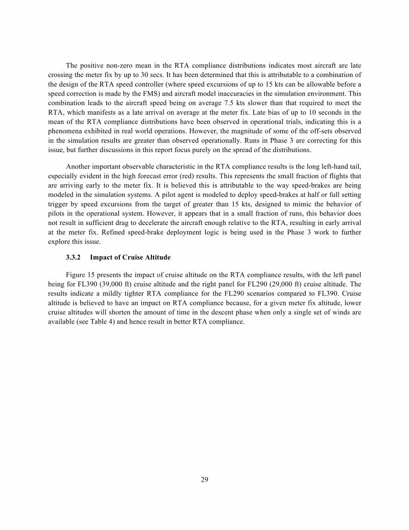
3.3.2 Impact of Cruise Altitude

Figure 15 presents the impact of cruise altitude on the RTA compliance results, with the left panel being for FL390 (39,000 ft) cruise altitude and the right panel for FL290 (29,000 ft) cruise altitude. The results indicate a mildly tighter RTA compliance for the FL290 scenarios compared to FL390. Cruise altitude is believed to have an impact on RTA compliance because, for a given meter fix altitude, lower cruise altitudes will shorten the amount of time in the descent phase when only a single set of winds are available (see Table 4) and hence result in better RTA compliance.

30

Figure 15. Impact of Cruise Altitude in Simulated 4D-TBO Scenarios

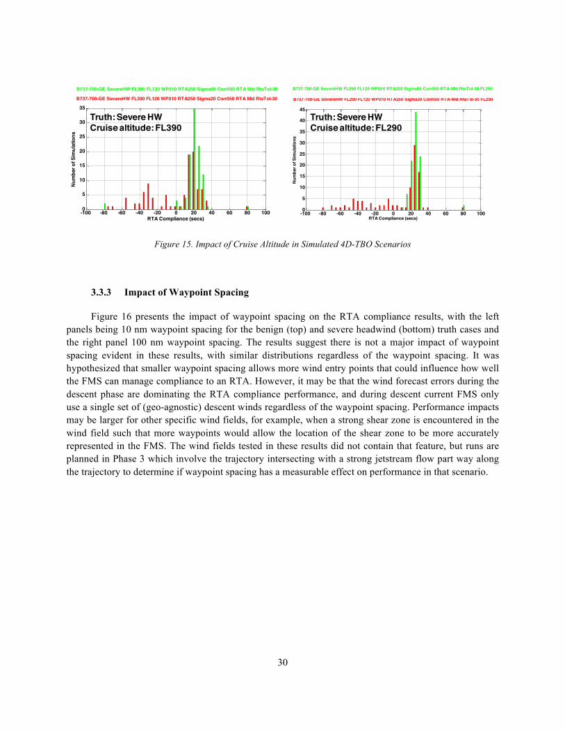
3.3.3 Impact of Waypoint Spacing

Figure 16 presents the impact of waypoint spacing on the RTA compliance results, with the left panels being 10 nm waypoint spacing for the benign (top) and severe headwind (bottom) truth cases and the right panel 100 nm waypoint spacing. The results suggest there is not a major impact of waypoint spacing evident in these results, with similar distributions regardless of the waypoint spacing. It was hypothesized that smaller waypoint spacing allows more wind entry points that could influence how well the FMS can manage compliance to an RTA. However, it may be that the wind forecast errors during the descent phase are dominating the RTA compliance performance, and during descent current FMS only use a single set of (geo-agnostic) descent winds regardless of the waypoint spacing. Performance impacts may be larger for other specific wind fields, for example, when a strong shear zone is encountered in the wind field such that more waypoints would allow the location of the shear zone to be more accurately represented in the FMS. The wind fields tested in these results did not contain that feature, but runs are planned in Phase 3 which involve the trajectory intersecting with a strong jetstream flow part way along the trajectory to determine if waypoint spacing has a measurable effect on performance in that scenario.



-100 -80 -60 -40 -20 0 20 40 60 80 1000

5

10

15

20

25

30

35


Num

ber o

f Sim

ulat

ions

1500 2000 2500 3000 3500 4000 45000

10

20

30

40

50

60


Num

ber o

f Sim

ulat

ions

05010015020025030060

70

80

90

100

110

120

130

140

Distance To Meter Fix (nm)H

eadw

ind

Expe

rienc

ed (k

ts)

0501001502002503001

1.5

2

2.5

3

3.5

4x 104


Alti

tude

(ft)



-100 -80 -60 -40 -20 0 20 40 60 80 1000

5

10

15

20

25

30

35


Num

ber o

f Sim

ulat

ions

1500 2000 2500 3000 3500 4000 45000

10

20

30

40

50

60


Num

ber o

f Sim

ulat

ions

05010015020025030060

70

80

90

100

110

120

130

140


Hea

dwin

d Ex

perie

nced

(kts

)

0501001502002503001

1.5

2

2.5

3

3.5

4x 104


Alti

tude

(ft)



-100 -80 -60 -40 -20 0 20 40 60 80 1000

5

10

15

20

25

30

35


Num

ber o

f Sim

ulat

ions

1500 2000 2500 3000 3500 4000 45000

10

20

30

40

50

60


Num

ber o

f Sim

ulat

ions

05010015020025030060

70

80

90

100

110

120

130

140


Hea

dwin

d Ex

perie

nced

(kts

)

0501001502002503001

1.5

2

2.5

3

3.5

4x 104


Alti

tude

(ft)

B737-700-GE SevereHW FL290 FL120 WP010 RTA250 Sigma05 Corr050 RTA-Mid RtaTol-30 FL290


0501001502002503001

1.5

2

2.5

3

3.5

4x 104


Alti

tude

(ft)

05010015020025030060

70

80

90

100

110

120

130

140


Hea

dwin

d Ex

perie

nced

(kts

)

1500 2000 2500 3000 3500 4000 45000

10

20

30

40

50

60

70

80

90

100


Num

ber o

f Sim

ulat

ions

-100 -80 -60 -40 -20 0 20 40 60 80 1000

5

10

15

20

25

30

35

40

45


Num

ber o

f Sim

ulat

ions



0501001502002503001

1.5

2

2.5

3

3.5

4x 104


Alti

tude

(ft)

05010015020025030060

70

80

90

100

110

120

130

140


Hea

dwin

d Ex

perie

nced

(kts

)

1500 2000 2500 3000 3500 4000 45000

10

20

30

40

50

60

70

80

90

100


Num

ber o

f Sim

ulat

ions

-100 -80 -60 -40 -20 0 20 40 60 80 1000

5

10

15

20

25

30

35

40

45


Num

ber o

f Sim

ulat

ions



0501001502002503001

1.5

2

2.5

3

3.5

4x 104


Alti

tude

(ft)

05010015020025030060

70

80

90

100

110

120

130

140


Hea

dwin

d Ex

perie

nced

(kts

)

1500 2000 2500 3000 3500 4000 45000

10

20

30

40

50

60

70

80

90

100


Num

ber o

f Sim

ulat

ions

-100 -80 -60 -40 -20 0 20 40 60 80 1000

5

10

15

20

25

30

35

40

45


Num

ber o

f Sim

ulat

ions

Truth: Severe HWCruise altitude: FL390

Truth: Severe HWCruise altitude: FL290

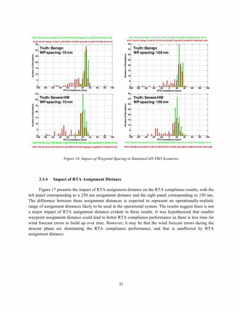
31

Figure 16. Impact of Waypoint Spacing in Simulated 4D-TBO Scenarios

3.3.4 Impact of RTA Assignment Distance

Figure 17 presents the impact of RTA assignment distance on the RTA compliance results, with the left panel corresponding to a 250 nm assignment distance and the right panel corresponding to 150 nm. The difference between these assignment distances is expected to represent an operationally-realistic range of assignment distances likely to be used in the operational system. The results suggest there is not a major impact of RTA assignment distance evident in these results. It was hypothesized that smaller waypoint assignment distance could lead to better RTA compliance performance as there is less time for wind forecast errors to build up over time. However, it may be that the wind forecast errors during the descent phase are dominating the RTA compliance performance, and that is unaffected by RTA assignment distance.



0501001502002503001

1.5

2

2.5

3

3.5

4x 104


Alti

tude

(ft)

050100150200250300

-15

-10

-5

0

5


eadw

ind

Expe

rienc

ed (k

ts)

1500 2000 2500 3000 3500 4000 45000

10

20

30

40

50

60

70

80


Num

ber o

f Sim

ulat

ions

-100 -80 -60 -40 -20 0 20 40 60 80 1000

5

10

15

20

25

30

35


Num

ber o

f Sim

ulat

ions



0501001502002503001

1.5

2

2.5

3

3.5

4x 104


Alti

tude

(ft)

050100150200250300

-15

-10

-5

0

5


Hea

dwin

d Ex

perie

nced

(kts

)

1500 2000 2500 3000 3500 4000 45000

10

20

30

40

50

60

70

80


Num

ber o

f Sim

ulat

ions

-100 -80 -60 -40 -20 0 20 40 60 80 1000

5

10

15

20

25

30

35


Num

ber o

f Sim

ulat

ions



0501001502002503001

1.5

2

2.5

3

3.5

4x 104


Alti

tude

(ft)

050100150200250300

-15

-10

-5

0

5


Hea

dwin

d Ex

perie

nced

(kts

)

1500 2000 2500 3000 3500 4000 45000

10

20

30

40

50

60

70

80


Num

ber o

f Sim

ulat

ions

-100 -80 -60 -40 -20 0 20 40 60 80 1000

5

10

15

20

25

30

35


Num

ber o

f Sim

ulat

ions



-100 -80 -60 -40 -20 0 20 40 60 80 1000

5

10

15

20

25

30

35


Num

ber o

f Sim

ulat

ions

1500 2000 2500 3000 3500 4000 45000

10

20

30

40

50

60


Num

ber o

f Sim

ulat

ions

05010015020025030060

70

80

90

100

110

120

130

140


Hea

dwin

d Ex

perie

nced

(kts

)

0501001502002503001

1.5

2

2.5

3

3.5

4x 104


Alti

tude

(ft)



-100 -80 -60 -40 -20 0 20 40 60 80 1000

5

10

15

20

25

30

35


Num

ber o

f Sim

ulat

ions

1500 2000 2500 3000 3500 4000 45000

10

20

30

40

50

60


Num

ber o

f Sim

ulat

ions

05010015020025030060

70

80

90

100

110

120

130

140


Hea

dwin

d Ex

perie

nced

(kts

)

0501001502002503001

1.5

2

2.5

3

3.5

4x 104


Alti

tude

(ft)



-100 -80 -60 -40 -20 0 20 40 60 80 1000

5

10

15

20

25

30

35


Num

ber o

f Sim

ulat

ions

1500 2000 2500 3000 3500 4000 45000

10

20

30

40

50

60


Num

ber o

f Sim

ulat

ions

05010015020025030060

70

80

90

100

110

120

130

140


Hea

dwin

d Ex

perie

nced

(kts

)

0501001502002503001

1.5

2

2.5

3

3.5

4x 104


Alti

tude

(ft)

Truth: BenignWP spacing: 10 nm

Truth: Severe HWWP spacing: 10 nm


B737-700-GE Benign FL390 FL120 WP100 RTA250 Sigma05 Corr050 RTA Mid Tol-30

0501001502002503001

1.5

2

2.5

3

3.5

4x 104


Alti

tude

(ft)

050100150200250300

-15

-10

-5

0

5


Hea

dwin

d Ex

perie

nced

(kts

)

1500 2000 2500 3000 3500 4000 45000

10

20

30

40

50

60

70

80

90


Num

ber o

f Sim

ulat

ions

-100 -80 -60 -40 -20 0 20 40 60 80 1000

5

10

15

20

25

30

35

40


Num

ber o

f Sim

ulat

ions



0501001502002503001

1.5

2

2.5

3

3.5

4x 104


Altit

ude

(ft)

050100150200250300

-15

-10

-5

0

5


Head

wind

Exp

erie

nced

(kts

)

1500 2000 2500 3000 3500 4000 45000

10

20

30

40

50

60

70

80

90


Num

ber o

f Sim

ulat

ions

-100 -80 -60 -40 -20 0 20 40 60 80 1000

5

10

15

20

25

30

35

40


Num

ber o

f Sim

ulat

ions



0501001502002503001

1.5

2

2.5

3

3.5

4x 104


Altit

ude

(ft)

050100150200250300

-15

-10

-5

0

5


Head

wind

Exp

erie

nced

(kts

)

1500 2000 2500 3000 3500 4000 45000

10

20

30

40

50

60

70

80

90


Num

ber o

f Sim

ulat

ions

-100 -80 -60 -40 -20 0 20 40 60 80 1000

5

10

15

20

25

30

35

40


Num

ber o

f Sim

ulat

ions

Truth: BenignWP spacing: 100 nm



0501001502002503001

1.5

2

2.5

3

3.5

4x 104


Alti

tude

(ft)

05010015020025030060

70

80

90

100

110

120

130

140


Hea

dwin

d Ex

perie

nced

(kts

)

1500 2000 2500 3000 3500 4000 45000

10

20

30

40

50

60

70


Num

ber o

f Sim

ulat

ions

-100 -80 -60 -40 -20 0 20 40 60 80 1000

5

10

15

20

25

30

35

40


Num

ber o

f Sim

ulat

ions



0501001502002503001

1.5

2

2.5

3

3.5

4x 104


Alti

tude

(ft)

05010015020025030060

70

80

90

100

110

120

130

140


Hea

dwin

d Ex

perie

nced

(kts

)

1500 2000 2500 3000 3500 4000 45000

10

20

30

40

50

60

70


Num

ber o

f Sim

ulat

ions

-100 -80 -60 -40 -20 0 20 40 60 80 1000

5

10

15

20

25

30

35

40


Num

ber o

f Sim

ulat

ions



0501001502002503001

1.5

2

2.5

3

3.5

4x 104

Distance To Meter Fix (nm)A

ltitu

de (f

t)050100150200250300

60

70

80

90

100

110

120

130

140


Hea

dwin

d Ex

perie

nced

(kts

)

1500 2000 2500 3000 3500 4000 45000

10

20

30

40

50

60

70


Num

ber o

f Sim

ulat

ions

-100 -80 -60 -40 -20 0 20 40 60 80 1000

5

10

15

20

25

30

35

40


Num

ber o

f Sim

ulat

ions

Truth: Severe HWWP spacing: 100 nm

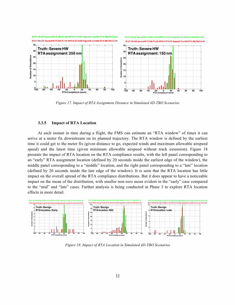
32

Figure 17. Impact of RTA Assignment Distance in Simulated 4D-TBO Scenarios

3.3.5 Impact of RTA Location

At each instant in time during a flight, the FMS can estimate an “RTA window” of times it can arrive at a meter fix downstream on its planned trajectory. The RTA window is defined by the earliest time it could get to the meter fix (given distance to go, expected winds and maximum allowable airspeed speed) and the latest time (given minimum allowable airspeed without track extension). Figure 18 presents the impact of RTA location on the RTA compliance results, with the left panel corresponding to an “early” RTA assignment location (defined by 20 seconds inside the earliest edge of the window), the middle panel corresponding to a “middle” location, and the right panel corresponding to a “late” location (defined by 20 seconds inside the late edge of the window). It is seen that the RTA location has little impact on the overall spread of the RTA compliance distributions. But it does appear to have a noticeable impact on the mean of the distribution, with smaller non-zero mean evident in the “early” case compared to the “mid” and “late” cases. Further analysis is being conducted in Phase 3 to explore RTA location effects in more detail.

Figure 18. Impact of RTA Location in Simulated 4D-TBO Scenarios

B737-700-GE SevereHW FL390 FL120 WP010 RTA150 Sigma05 Corr050 RTA-Mid RtaTol-30


0501001502002503001

1.5

2

2.5

3

3.5

4x 104


Alti

tude

(ft)

050100150200250300

60

70

80

90

100

110

120

130

140


Hea

dwin

d Ex

perie

nced

(kts

)

1500 2000 2500 3000 3500 4000 45000

10

20

30

40

50

60

70

80

90

100


Num

ber o

f Sim

ulat

ions

-100 -80 -60 -40 -20 0 20 40 60 80 1000

5

10

15

20

25

30

35


Num

ber o

f Sim

ulat

ions



-100 -80 -60 -40 -20 0 20 40 60 80 1000

5

10

15

20

25

30

35


Num

ber o

f Sim

ulat

ions

1500 2000 2500 3000 3500 4000 45000

10

20

30

40

50

60


Num

ber o

f Sim

ulat

ions

05010015020025030060

70

80

90

100

110

120

130

140


eadw

ind

Expe

rienc

ed (k

ts)

0501001502002503001

1.5

2

2.5

3

3.5

4x 104


Alti

tude

(ft)



-100 -80 -60 -40 -20 0 20 40 60 80 1000

5

10

15

20

25

30

35


Num

ber o

f Sim

ulat

ions

1500 2000 2500 3000 3500 4000 45000

10

20

30

40

50

60


Num

ber o

f Sim

ulat

ions

05010015020025030060

70

80

90

100

110

120

130

140


Hea

dwin

d Ex

perie

nced

(kts

)

0501001502002503001

1.5

2

2.5

3

3.5

4x 104


Alti

tude

(ft)



-100 -80 -60 -40 -20 0 20 40 60 80 1000

5

10

15

20

25

30

35


Num

ber o

f Sim

ulat

ions

1500 2000 2500 3000 3500 4000 45000

10

20

30

40

50

60


Num

ber o

f Sim

ulat

ions

05010015020025030060

70

80

90

100

110

120

130

140


Hea

dwin

d Ex

perie

nced

(kts

)

0501001502002503001

1.5

2

2.5

3

3.5

4x 104


Alti

tude

(ft)

Truth: Severe HWRTA assignment: 250 nm

Truth: Severe HWRTA assignment: 150 nm



0501001502002503001

1.5

2

2.5

3

3.5

4x 104


Alti

tude

(ft)

050100150200250300

60

70

80

90

100

110

120

130

140


Hea

dwin

d Ex

perie

nced

(kts

)

1500 2000 2500 3000 3500 4000 45000

10

20

30

40

50

60

70

80

90

100


Num

ber o

f Sim

ulat

ions

-100 -80 -60 -40 -20 0 20 40 60 80 1000

5

10

15

20

25

30

35


Num

ber o

f Sim

ulat

ions



0501001502002503001

1.5

2

2.5

3

3.5

4x 104


Alti

tude

(ft)

050100150200250300

60

70

80

90

100

110

120

130

140


Hea

dwin

d Ex

perie

nced

(kts

)

1500 2000 2500 3000 3500 4000 45000

10

20

30

40

50

60

70

80

90

100


Num

ber o

f Sim

ulat

ions

-100 -80 -60 -40 -20 0 20 40 60 80 1000

5

10

15

20

25

30

35


Num

ber o

f Sim

ulat

ions



0501001502002503001

1.5

2

2.5

3

3.5

4x 104


Alti

tude

(ft)

050100150200250300

-15

-10

-5

0

5


Hea

dwin

d Ex

perie

nced

(kts

)

1500 2000 2500 3000 3500 4000 45000

10

20

30

40

50

60

70

80


Num

ber o

f Sim

ulat

ions

-100 -80 -60 -40 -20 0 20 40 60 80 1000

5

10

15

20

25

30

35


Num

ber o

f Sim

ulat

ions



0501001502002503001

1.5

2

2.5

3

3.5

4x 104


Alti

tude

(ft)

050100150200250300

-15

-10

-5

0

5


Hea

dwin

d Ex

perie

nced

(kts

)

1500 2000 2500 3000 3500 4000 45000

10

20

30

40

50

60

70

80


Num

ber o

f Sim

ulat

ions

-100 -80 -60 -40 -20 0 20 40 60 80 1000

5

10

15

20

25

30

35


Num

ber o

f Sim

ulat

ions



0501001502002503001

1.5

2

2.5

3

3.5

4x 104


Alti

tude

(ft)

050100150200250300

-15

-10

-5

0

5


Hea

dwin

d Ex

perie

nced

(kts

)

1500 2000 2500 3000 3500 4000 45000

10

20

30

40

50

60

70

80


Num

ber o

f Sim

ulat

ions

-100 -80 -60 -40 -20 0 20 40 60 80 1000

5

10

15

20

25

30

35


Num

ber o

f Sim

ulat

ions

Truth: BenignRTA location: Mid

B737-700-GE Benign FL390 FL120 WP010 RTA250 Sigma05 Corr050 RTA-Early RtaTol-30


0501001502002503001

1.5

2

2.5

3

3.5

4x 104


Alti

tude

(ft)

050100150200250300

-15

-10

-5

0


Hea

dwin

d Ex

perie

nced

(kts

)

1500 2000 2500 3000 3500 4000 45000

2

4

6

8

10

12

14

16


Num

ber o

f Sim

ulat

ions

-100 -80 -60 -40 -20 0 20 40 60 80 1000

1

2

3

4

5

6

7

8

9


Num

ber o

f Sim

ulat

ions



0501001502002503001

1.5

2

2.5

3

3.5

4x 104


Alti

tude

(ft)

050100150200250300

-15

-10

-5

0


Hea

dwin

d Ex

perie

nced

(kts

)

1500 2000 2500 3000 3500 4000 45000

2

4

6

8

10

12

14

16


Num

ber o

f Sim

ulat

ions

-100 -80 -60 -40 -20 0 20 40 60 80 1000

1

2

3

4

5

6

7

8

9


Num

ber o

f Sim

ulat

ions



0501001502002503001

1.5

2

2.5

3

3.5

4x 104


Alti

tude

(ft)

050100150200250300

-15

-10

-5

0


Hea

dwin

d Ex

perie

nced

(kts

)

1500 2000 2500 3000 3500 4000 45000

2

4

6

8

10

12

14

16


Num

ber o

f Sim

ulat

ions

-100 -80 -60 -40 -20 0 20 40 60 80 1000

1

2

3

4

5

6

7

8

9


Num

ber o

f Sim

ulat

ions

Truth: BenignRTA location: Early

B737-700-GE Benign FL390 FL120 WP010 RTA250 Sigma05 Corr050 RTA-Late RtaTol-30


0501001502002503001

1.5

2

2.5

3

3.5

4x 104


Alti

tude

(ft)

050100150200250300

-15

-10

-5

0

5


Hea

dwin

d Ex

perie

nced

(kts

)

1500 2000 2500 3000 3500 4000 45000

5

10

15

20

25


Num

ber o

f Sim

ulat

ions

-100 -80 -60 -40 -20 0 20 40 60 80 1000

2

4

6

8

10


Num

ber o

f Sim

ulat

ions



0501001502002503001

1.5

2

2.5

3

3.5

4x 104


Alti

tude

(ft)

050100150200250300

-15

-10

-5

0

5


Hea

dwin

d Ex

perie

nced

(kts

)

1500 2000 2500 3000 3500 4000 45000

5

10

15

20

25


Num

ber o

f Sim

ulat

ions

-100 -80 -60 -40 -20 0 20 40 60 80 1000

2

4

6

8

10


Num

ber o

f Sim

ulat

ions



0501001502002503001

1.5

2

2.5

3

3.5

4x 104


Alti

tude

(ft)

050100150200250300

-15

-10

-5

0

5


Hea

dwin

d Ex

perie

nced

(kts

)

1500 2000 2500 3000 3500 4000 45000

5

10

15

20

25


Num

ber o

f Sim

ulat

ions

-100 -80 -60 -40 -20 0 20 40 60 80 1000

2

4

6

8

10


Num

ber o

f Sim

ulat

ions

Truth: BenignRTA location: Late

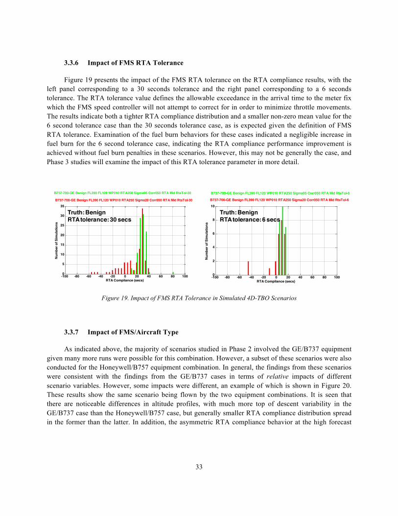
33

3.3.6 Impact of FMS RTA Tolerance

Figure 19 presents the impact of the FMS RTA tolerance on the RTA compliance results, with the left panel corresponding to a 30 seconds tolerance and the right panel corresponding to a 6 seconds tolerance. The RTA tolerance value defines the allowable exceedance in the arrival time to the meter fix which the FMS speed controller will not attempt to correct for in order to minimize throttle movements. The results indicate both a tighter RTA compliance distribution and a smaller non-zero mean value for the 6 second tolerance case than the 30 seconds tolerance case, as is expected given the definition of FMS RTA tolerance. Examination of the fuel burn behaviors for these cases indicated a negligible increase in fuel burn for the 6 second tolerance case, indicating the RTA compliance performance improvement is achieved without fuel burn penalties in these scenarios. However, this may not be generally the case, and Phase 3 studies will examine the impact of this RTA tolerance parameter in more detail.

Figure 19. Impact of FMS RTA Tolerance in Simulated 4D-TBO Scenarios

3.3.7 Impact of FMS/Aircraft Type

As indicated above, the majority of scenarios studied in Phase 2 involved the GE/B737 equipment given many more runs were possible for this combination. However, a subset of these scenarios were also conducted for the Honeywell/B757 equipment combination. In general, the findings from these scenarios were consistent with the findings from the GE/B737 cases in terms of relative impacts of different scenario variables. However, some impacts were different, an example of which is shown in Figure 20. These results show the same scenario being flown by the two equipment combinations. It is seen that there are noticeable differences in altitude profiles, with much more top of descent variability in the GE/B737 case than the Honeywell/B757 case, but generally smaller RTA compliance distribution spread in the former than the latter. In addition, the asymmetric RTA compliance behavior at the high forecast



0501001502002503001

1.5

2

2.5

3

3.5

4x 104


Alti

tude

(ft)

050100150200250300

-15

-10

-5

0

5


Hea

dwin

d Ex

perie

nced

(kts

)

1500 2000 2500 3000 3500 4000 45000

10

20

30

40

50

60

70

80


Num

ber o

f Sim

ulat

ions

-100 -80 -60 -40 -20 0 20 40 60 80 1000

5

10

15

20

25

30

35


Num

ber o

f Sim

ulat

ions



0501001502002503001

1.5

2

2.5

3

3.5

4x 104


Alti

tude

(ft)

050100150200250300

-15

-10

-5

0

5


Hea

dwin

d Ex

perie

nced

(kts

)

1500 2000 2500 3000 3500 4000 45000

10

20

30

40

50

60

70

80


Num

ber o

f Sim

ulat

ions

-100 -80 -60 -40 -20 0 20 40 60 80 1000

5

10

15

20

25

30

35


Num

ber o

f Sim

ulat

ions



0501001502002503001

1.5

2

2.5

3

3.5

4x 104


Alti

tude

(ft)

050100150200250300

-15

-10

-5

0

5


eadw

ind

Expe

rienc

ed (k

ts)

1500 2000 2500 3000 3500 4000 45000

10

20

30

40

50

60

70

80


Num

ber o

f Sim

ulat

ions

-100 -80 -60 -40 -20 0 20 40 60 80 1000

5

10

15

20

25

30

35


Num

ber o

f Sim

ulat

ions

Truth: BenignRTA tolerance: 30 secs



0501001502002503001

1.5

2

2.5

3

3.5

4x 104


Alti

tude

(ft)

050100150200250300

-15

-10

-5

0

5


Hea

dwin

d Ex

perie

nced

(kts

)

1500 2000 2500 3000 3500 4000 45000

5

10

15

20


Num

ber o

f Sim

ulat

ions

-100 -80 -60 -40 -20 0 20 40 60 80 1000

2

4

6

8

10


Num

ber o

f Sim

ulat

ions



0501001502002503001

1.5

2

2.5

3

3.5

4x 104


Alti

tude

(ft)

050100150200250300

-15

-10

-5

0

5


Hea

dwin

d Ex

perie

nced

(kts

)

1500 2000 2500 3000 3500 4000 45000

5

10

15

20


Num

ber o

f Sim

ulat

ions

-100 -80 -60 -40 -20 0 20 40 60 80 1000

2

4

6

8

10


Num

ber o

f Sim

ulat

ions



0501001502002503001

1.5

2

2.5

3

3.5

4x 104


Alti

tude

(ft)

050100150200250300

-15

-10

-5

0

5


Hea

dwin

d Ex

perie

nced

(kts

)

1500 2000 2500 3000 3500 4000 45000

5

10

15

20


Num

ber o

f Sim

ulat

ions

-100 -80 -60 -40 -20 0 20 40 60 80 1000

2

4

6

8

10


Num

ber o

f Sim

ulat

ions

Truth: BenignRTA tolerance: 6 secs

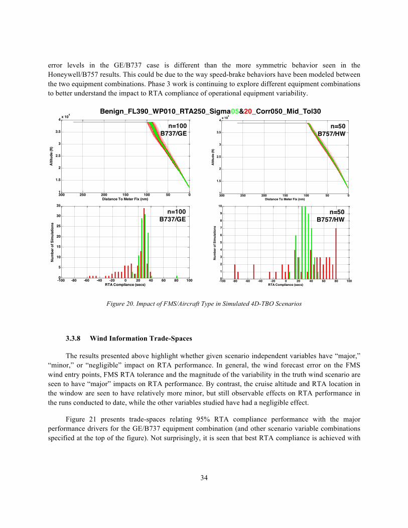
34

error levels in the GE/B737 case is different than the more symmetric behavior seen in the Honeywell/B757 results. This could be due to the way speed-brake behaviors have been modeled between the two equipment combinations. Phase 3 work is continuing to explore different equipment combinations to better understand the impact to RTA compliance of operational equipment variability.

Figure 20. Impact of FMS/Aircraft Type in Simulated 4D-TBO Scenarios

3.3.8 Wind Information Trade-Spaces

The results presented above highlight whether given scenario independent variables have “major,” “minor,” or “negligible” impact on RTA performance. In general, the wind forecast error on the FMS wind entry points, FMS RTA tolerance and the magnitude of the variability in the truth wind scenario are seen to have “major” impacts on RTA performance. By contrast, the cruise altitude and RTA location in the window are seen to have relatively more minor, but still observable effects on RTA performance in the runs conducted to date, while the other variables studied have had a negligible effect.

Figure 21 presents trade-spaces relating 95% RTA compliance performance with the major performance drivers for the GE/B737 equipment combination (and other scenario variable combinations specified at the top of the figure). Not surprisingly, it is seen that best RTA compliance is achieved with



0501001502002503001

1.5

2

2.5

3

3.5

4x 104


Alti

tude

(ft)

050100150200250300

-15

-10

-5

0

5


Hea

dwin

d Ex

perie

nced

(kts

)

1500 2000 2500 3000 3500 4000 45000

10

20

30

40

50

60

70

80


Num

ber o

f Sim

ulat

ions

-100 -80 -60 -40 -20 0 20 40 60 80 1000

5

10

15

20

25

30

35


Num

ber o

f Sim

ulat

ions

Benign_FL390_WP010_RTA250_Sigma05&20_Corr050_Mid_Tol30



0501001502002503001

1.5

2

2.5

3

3.5

4x 104


Alti

tude

(ft)

050100150200250300

-15

-10

-5

0

5


Hea

dwin

d Ex

perie

nced

(kts

)

1500 2000 2500 3000 3500 4000 45000

10

20

30

40

50

60

70

80


Num

ber o

f Sim

ulat

ions

-100 -80 -60 -40 -20 0 20 40 60 80 1000

5

10

15

20

25

30

35


Num

ber o

f Sim

ulat

ions

n=100B737/GE

n=100B737/GE

B757-HW-BL Benign FL390 FL120 WP010 RTA250 Sigma05 Corr050RTA-MidRtaTol-30


0501001502002503001

1.5

2

2.5

3

3.5

4x 104


Alti

tude

(ft)

050100150200250300-16

-14

-12

-10

-8

-6

-4

-2

0

2

4


Hea

dwin

d Ex

perie

nced

(kts

)

-100 -80 -60 -40 -20 0 20 40 60 80 1000

1

2

3

4

5

6

7

8

9

10


Num

ber o

f Sim

ulat

ions



0501001502002503001

1.5

2

2.5

3

3.5

4x 104


Alti

tude

(ft)

050100150200250300-16

-14

-12

-10

-8

-6

-4

-2

0

2

4


Hea

dwin

d Ex

perie

nced

(kts

)

-100 -80 -60 -40 -20 0 20 40 60 80 1000

1

2

3

4

5

6

7

8

9

10


Num

ber o

f Sim

ulat

ions

n=50B757/HW

n=50B757/HW

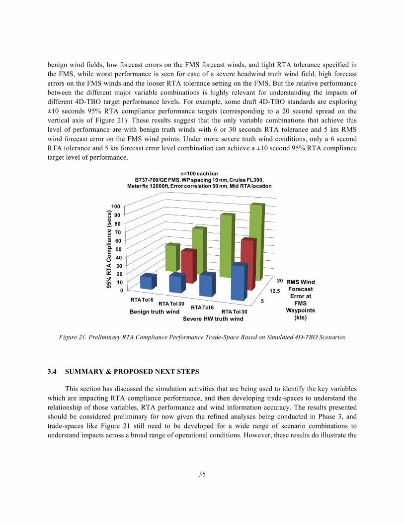
35

benign wind fields, low forecast errors on the FMS forecast winds, and tight RTA tolerance specified in the FMS, while worst performance is seen for case of a severe headwind truth wind field, high forecast errors on the FMS winds and the looser RTA tolerance setting on the FMS. But the relative performance between the different major variable combinations is highly relevant for understanding the impacts of different 4D-TBO target performance levels. For example, some draft 4D-TBO standards are exploring ±10 seconds 95% RTA compliance performance targets (corresponding to a 20 second spread on the vertical axis of Figure 21). These results suggest that the only variable combinations that achieve this level of performance are with benign truth winds with 6 or 30 seconds RTA tolerance and 5 kts RMS wind forecast error on the FMS wind points. Under more severe truth wind conditions, only a 6 second RTA tolerance and 5 kts forecast error level combination can achieve a ±10 second 95% RTA compliance target level of performance.

Figure 21. Preliminary RTA Compliance Performance Trade-Space Based on Simulated 4D-TBO Scenarios


This section has discussed the simulation activities that are being used to identify the key variables which are impacting RTA compliance performance, and then developing trade-spaces to understand the relationship of those variables, RTA performance and wind information accuracy. The results presented should be considered preliminary for now given the refined analyses being conducted in Phase 3, and trade-spaces like Figure 21 still need to be developed for a wide range of scenario combinations to understand impacts across a broad range of operational conditions. However, these results do illustrate the

7

17.5

28

0102030405060708090

100

RTA Tol 6RTA Tol 30

RTA Tol 6RTA Tol 30

n=100 each barB737-700/GE FMS, WP spacing 10 nm, Cruise FL390,

Meter fix 12000ft, Error correlation 50 nm, Mid RTA location

Benign truth windSevere HW truth wind

RMS WindForecastError at

FMSWaypoints

(kts)

95%

RTA

Com

plia

nce

(sec

s)

5

12.5

20

36

insights that can be gained from this type of trade-space which, unlike in Phase 1, are now based on high fidelity models of the different elements of the analysis framework.

In terms of next steps, the main objective for Phase 3 is to develop sets of refined trade-spaces relating RTA compliance performance to major performance drivers for both GE/B737 and Honeywell/B757 equipment across a broad range of operational conditions. This will include focused additional simulations with benign, moderate, severe, and extreme truth wind scenarios which have been defined based on a metric which accounts for the location of wind forecast error relative to the meter fix location. As indicated in the respective subsections above, more study is also required to fully define what (and under what conditions) the major, minor, and negligible scenario variables are which impact RTA performance. It is anticipated that the Phase 3 trade-spaces will be defined based primarily on the major performance drivers, but the impact of minor performance drivers will be quantified with uncertainty bars on the trade-space elements where appropriate. Finally, once the refined trade-spaces have been defined, additional steps will be conducted in Phase 3 to interpret their implication to wind information needs to reach a target RTA compliance performance. As illustrated in the insights provided from the initial trade-space of Figure 21, the trade-spaces can be used to translate a required RTA performance into maximum allowable wind forecast RMS error level in the FMS. As shown in the far right box of the analysis framework (see Figure 2), this wind accuracy requirement can, in turn, be used to define combinations of operational-relevant variables such as wind data content, accuracy, precision and update rate provided to the FMS to achieve wind errors below this maximum allowable level. It is hoped that such information will be of high value in the development of concepts of operation, performance target and datalink requirement setting activities currently being conducted by stakeholders.

37

4. WIND INFORMATION ANALYSIS FOR 4D-TBO APPLICATIONS WITH FUTURE FMS

4.1 INTRODUCTION

Work on FMS enhancements undertaken during this phase of research focused on incremental enhancements to wind blending algorithms in current FMSs to enable quantification of performance improvement potential from near-term avionics refinements. A competitive process to identify collaborators resulted in a contract award to Honeywell to support this task. Thus far, Honeywell have provided three versions of FMS software to support this research:

• B757/767 Pegasus FMS using current operational (“Black Label”) software, which provides full RTA utility only during cruise. Time constraints on a waypoint can be specified that include a climb or descent segment, but speeds are actively managed to achieve the time constraint only during cruise.

• B757/767 Pegasus FMS using research prototype (“Red Label”) software, which provides full RTA utility during all phases of flight and other enhancements.

• B757/767 Pegasus FMS using research prototype software plus enhancements to the wind blending algorithms employed (“Enhanced WB”). Wind blending is the mechanism by which corrections are made to downstream waypoint wind entries as function of the magnitude of the errors between the sensed and forecast wind at the current location. This algorithm was considered to be one of the main opportunities for FMS performance improvement, hence the focus of our initial enhancement assessment.

MIT Lincoln Laboratory developed an aircraft/FMS simulation architecture to implement the different Honeywell FMS software for scripted scenarios to evaluate the proposed enhancements and quantify FMS performance for 4D-TBO applications. Details on the enhancements to the wind blending algorithms, aircraft/FMS architecture and implementation, and results of the analysis are presented in this section.

4.2 FMS ENHANCEMENTS OVERVIEW

FMS systems employed in air transport aircraft implement some form of “wind blending” to mitigate adverse impacts of wind forecast uncertainty and/or stale or incorrect wind forecasts loaded into the FMS. In wind blending, the current sensed or measured wind is applied by algorithm to the forecast to determine the predicted wind at points ahead of the aircraft on the flight plan route for trajectory calculations and predictions. Typically, the algorithm functions such that the measured wind is more heavily weighted in short range calculations, and forecast wind becomes progressively more heavily

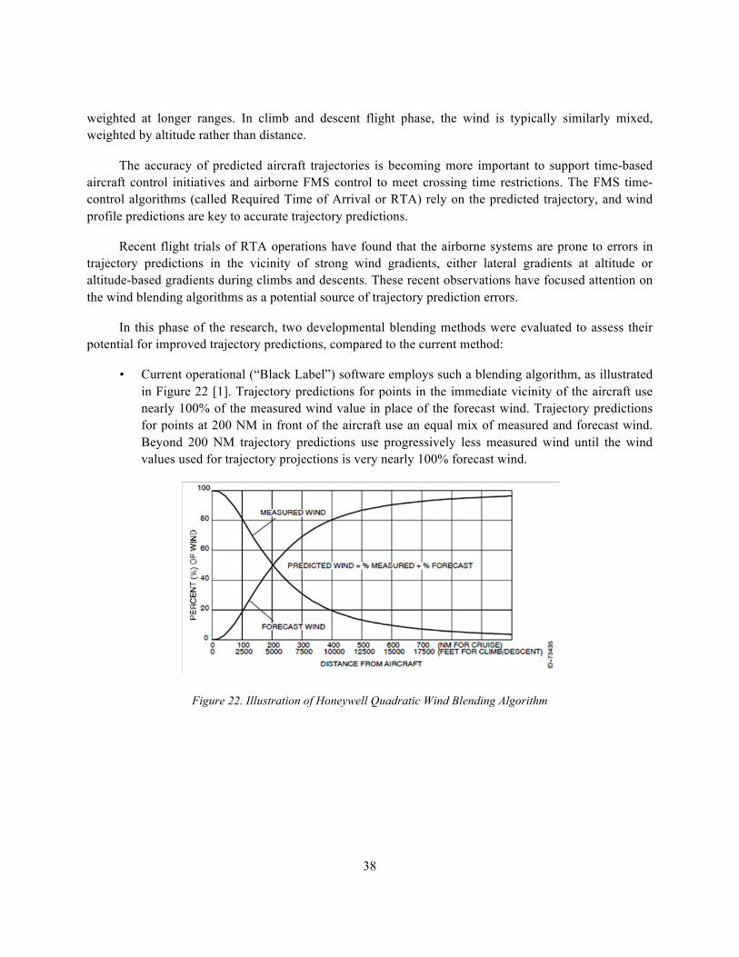
38

weighted at longer ranges. In climb and descent flight phase, the wind is typically similarly mixed, weighted by altitude rather than distance.

The accuracy of predicted aircraft trajectories is becoming more important to support time-based aircraft control initiatives and airborne FMS control to meet crossing time restrictions. The FMS time-control algorithms (called Required Time of Arrival or RTA) rely on the predicted trajectory, and wind profile predictions are key to accurate trajectory predictions.

Recent flight trials of RTA operations have found that the airborne systems are prone to errors in trajectory predictions in the vicinity of strong wind gradients, either lateral gradients at altitude or altitude-based gradients during climbs and descents. These recent observations have focused attention on the wind blending algorithms as a potential source of trajectory prediction errors.

In this phase of the research, two developmental blending methods were evaluated to assess their potential for improved trajectory predictions, compared to the current method:

• Current operational (“Black Label”) software employs such a blending algorithm, as illustrated in Figure 22 [1]. Trajectory predictions for points in the immediate vicinity of the aircraft use nearly 100% of the measured wind value in place of the forecast wind. Trajectory predictions for points at 200 NM in front of the aircraft use an equal mix of measured and forecast wind. Beyond 200 NM trajectory predictions use progressively less measured wind until the wind values used for trajectory projections is very nearly 100% forecast wind.

Figure 22. Illustration of Honeywell Quadratic Wind Blending Algorithm

39

• An initial version of the research prototype software (“Red Label”) employed a revised blending algorithm to limit the extrapolation of the measured wind down range to preserve the gradient characteristics of the wind forecast.

• An updated version of the research prototype software (“Enhanced WB”) employed an enhancement of the revised blending algorithm in such a way that the sensed wind values are used to improve the accuracy of the forecast, not to replace the forecasts at downstream points.

Honeywell provided “option switches” coded into a MAINT function of the FMS to permit down selection of the blending algorithm to be used for data runs, limited by the algorithm versions included in the particular software build.

• B757/767 Pegasus FMS using current operational (“Black Label”) software includes only the quadratic blending method that must be used for all runs.

• B757/767 Pegasus FMS using the initial research prototype software (“Red Label”) defaults to the revised blending method; the current method can be used for data runs.

• B757/767 Pegasus FMS using the updated research prototype software (“Enhanced WB”) defaults to the enhanced revised blending method; the other methods can be used for data runs.

An initial assessment of these methods by Honeywell indicated substantive potential from proposed incremental enhancements to wind blending algorithms applied to two cases: 1) matched winds in the presence of wind gradients (sensed winds match forecast winds, winds change over distance or altitude), so any divergence from actual values would be consequence of the intrinsic behavior of the algorithm; 2) mismatched winds in the presence of wind gradients (modest error in forecast winds), so the blending algorithm would apply the sensed winds to mitigate the adverse impacts of the forecast error.

For both cases:

• Predicted wind values from the current operational blending algorithm diverge from the forecast, attributed to the extrapolation of the measured wind too far downstream.

• The revised blending algorithm limited the downstream extrapolation of the measured wind and the divergence from the forecast.

• The enhanced revised blending algorithm, seemed to eliminate the divergence observed using the other blending algorithms.

Since the RTA function is a closed-loop feedback system that continues to operate as the aircraft approaches the time constraint waypoint, the current wind blending algorithm can usually meet the arrival time constraint because the system feedback acts to mitigate the modeling errors. However, there are

40

several aspects of the RTA functional performance that are expected to improve with the introduction of the developmental blending methods:

• Improved accuracy of “UNABLE RTA” alert through more timely recognition of performance trends indicating that the time constraint will not be met and reduced “false alerts” through improved handling of trajectory predictions in areas of forecast wind gradients;

• Reduced disturbances in the RTA feedback control loop, improving the functional performance of the RTA function;

• Earlier speed adjustments and more stable speed profiles to keep the predicted trajectory within the achievable performance envelope of the aircraft;

• Improved arrival time accuracy when there is a wind gradient in the vicinity of the time constraint waypoint.

Preliminary results indicate substantive potential from proposed incremental enhancements to wind blending algorithms (see Section 4.4), and it is planned to expand on this with multiple data runs using the MIT LL aircraft/FMS emulator in a broad sample of test cases (see Section 4.5).

4.3 FMS/AIRCRAFT SIMULATION ARCHITECTURE

4.3.1 Objectives

The design objectives of the simulation architecture were; 1) that it must be able to integrate a physical or logical representation of a commercially available FMS used in industry; 2) that the components of the system are modular; 3) that the components of the system are as accurate as practical in characteristics relevant to the study and 4) that the system must be scalable. Each of these design objectives has been achieved.

The simulation system is figuratively world encompassing. It includes geographical models of the Earth and each of the relevant subsystem embedded within it. Relevant subsystems are those entities that are believed to affect the outcomes of the research efforts. Each of the components in the simulation, sometimes called agents, are composed of one or more subsystem. Each subsystem can communicate with other simulation elements utilizing a common communication mechanism on a shared logical data bus. Utilizing this type of communication mechanism creates loose-coupling between modeled elements and permits considerable flexibility in the overall system. Each agent is executed as a separate process when possible and appropriate.

One of the advantages of this architecture is that it permits plug-and-play substitution of agents in the system as more sophisticated models are developed or when alternate characteristics are desired. It also provides the unobstructed inspection and monitoring of agent activity which is valuable for system and performance analysis. The use of the shared data bus and the placement of critical elements of the

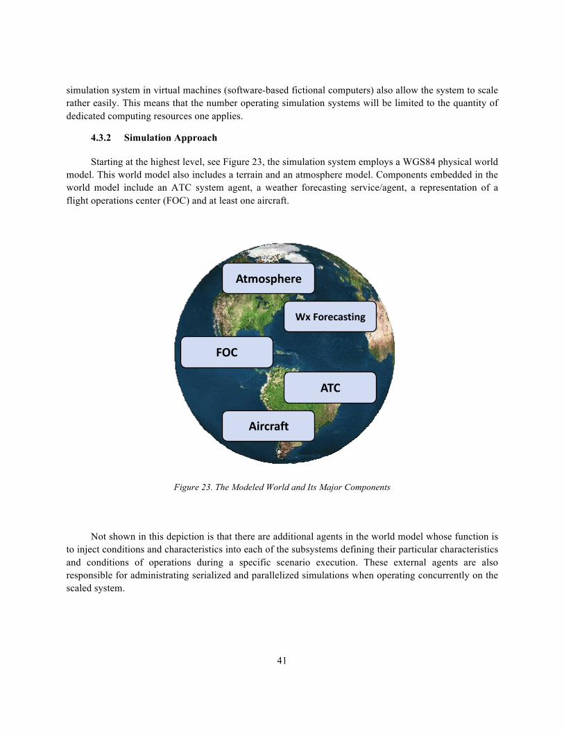
41

simulation system in virtual machines (software-based fictional computers) also allow the system to scale rather easily. This means that the number operating simulation systems will be limited to the quantity of dedicated computing resources one applies.

4.3.2 Simulation Approach

Starting at the highest level, see Figure 23, the simulation system employs a WGS84 physical world model. This world model also includes a terrain and an atmosphere model. Components embedded in the world model include an ATC system agent, a weather forecasting service/agent, a representation of a flight operations center (FOC) and at least one aircraft.

Figure 23. The Modeled World and Its Major Components

Not shown in this depiction is that there are additional agents in the world model whose function is to inject conditions and characteristics into each of the subsystems defining their particular characteristics and conditions of operations during a specific scenario execution. These external agents are also responsible for administrating serialized and parallelized simulations when operating concurrently on the scaled system.

Aircraft

Atmosphere

FOC

Wx Forecasting

ATC

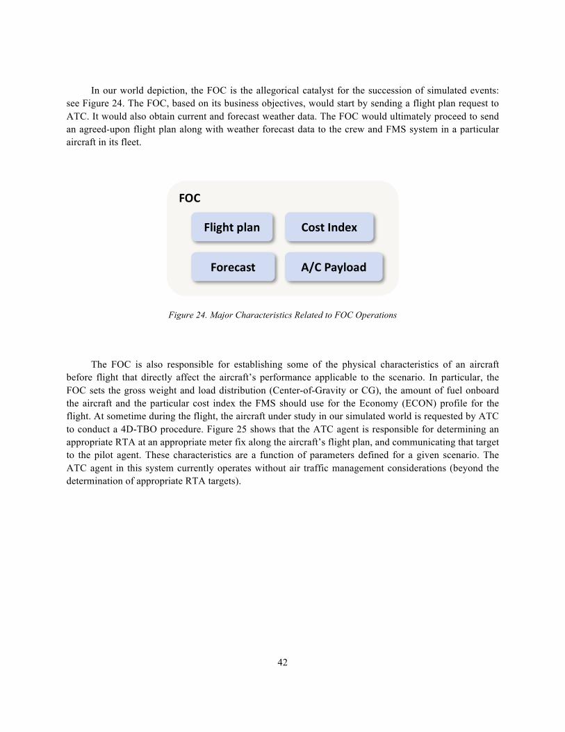
42

In our world depiction, the FOC is the allegorical catalyst for the succession of simulated events: see Figure 24. The FOC, based on its business objectives, would start by sending a flight plan request to ATC. It would also obtain current and forecast weather data. The FOC would ultimately proceed to send an agreed-upon flight plan along with weather forecast data to the crew and FMS system in a particular aircraft in its fleet.

Figure 24. Major Characteristics Related to FOC Operations

The FOC is also responsible for establishing some of the physical characteristics of an aircraft before flight that directly affect the aircraft’s performance applicable to the scenario. In particular, the FOC sets the gross weight and load distribution (Center-of-Gravity or CG), the amount of fuel onboard the aircraft and the particular cost index the FMS should use for the Economy (ECON) profile for the flight. At sometime during the flight, the aircraft under study in our simulated world is requested by ATC to conduct a 4D-TBO procedure. Figure 25 shows that the ATC agent is responsible for determining an appropriate RTA at an appropriate meter fix along the aircraft’s flight plan, and communicating that target to the pilot agent. These characteristics are a function of parameters defined for a given scenario. The ATC agent in this system currently operates without air traffic management considerations (beyond the determination of appropriate RTA targets).

FOC

Flight plan Cost Index

Forecast A/C Payload

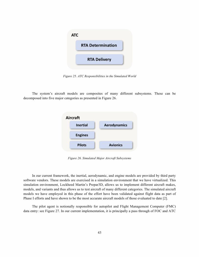
43

Figure 25. ATC Responsibilities in the Simulated World

The system’s aircraft models are composites of many different subsystems. These can be decomposed into five major categories as presented in Figure 26.

Figure 26. Simulated Major Aircraft Subsystems

In our current framework, the inertial, aerodynamic, and engine models are provided by third party software vendors. These models are exercised in a simulation environment that we have virtualized. This simulation environment, Lockheed Martin’s Prepar3D, allows us to implement different aircraft makes, models, and variants and thus allows us to test aircraft of many different categories. The simulated aircraft models we have employed in this phase of the effort have been validated against flight data as part of Phase I efforts and have shown to be the most accurate aircraft models of those evaluated to date [2].

The pilot agent is notionally responsible for autopilot and Flight Management Computer (FMC) data entry: see Figure 27. In our current implementation, it is principally a pass through of FOC and ATC

ATC

RTA Determination

RTA Delivery

Aircraft

Aerodynamics

Avionics

Inertial

Engines

Pilots

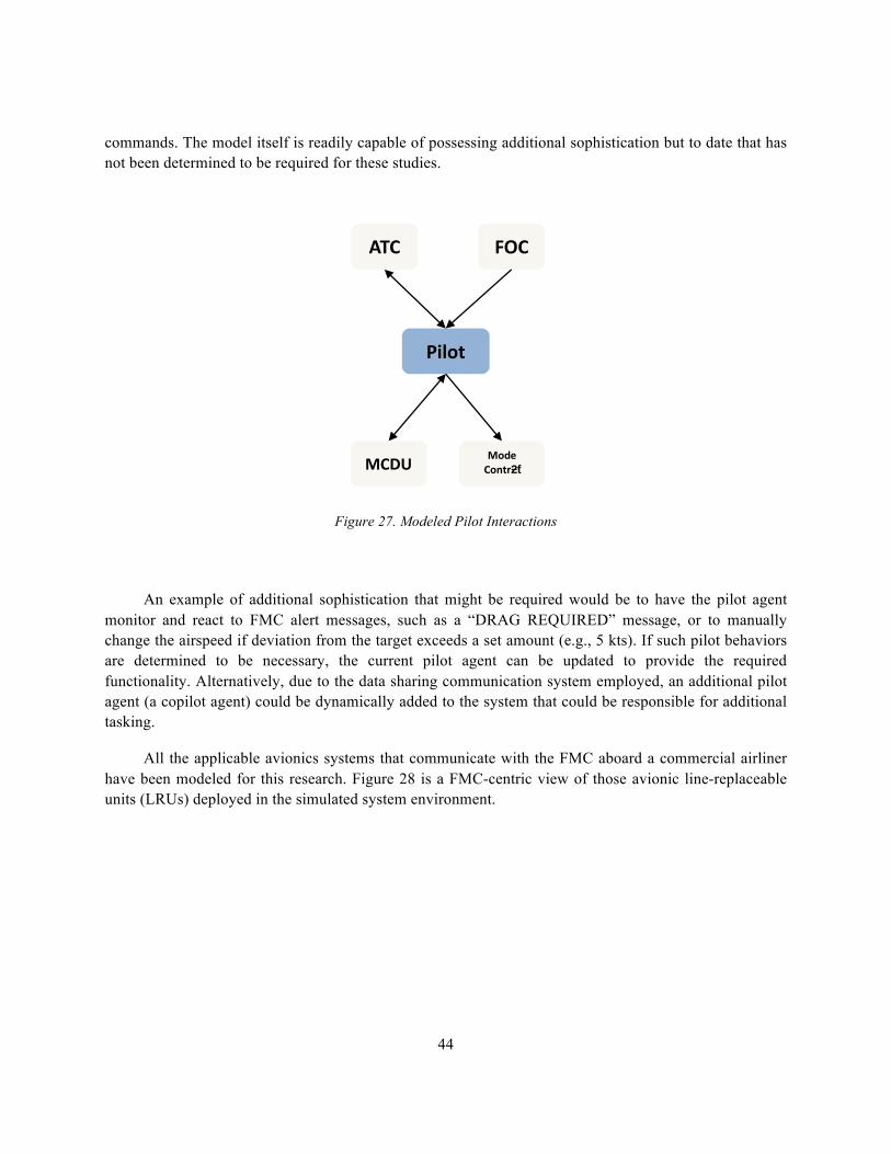
44

commands. The model itself is readily capable of possessing additional sophistication but to date that has not been determined to be required for these studies.

Figure 27. Modeled Pilot Interactions

An example of additional sophistication that might be required would be to have the pilot agent monitor and react to FMC alert messages, such as a “DRAG REQUIRED” message, or to manually change the airspeed if deviation from the target exceeds a set amount (e.g., 5 kts). If such pilot behaviors are determined to be necessary, the current pilot agent can be updated to provide the required functionality. Alternatively, due to the data sharing communication system employed, an additional pilot agent (a copilot agent) could be dynamically added to the system that could be responsible for additional tasking.

All the applicable avionics systems that communicate with the FMC aboard a commercial airliner have been modeled for this research. Figure 28 is a FMC-centric view of those avionic line-replaceable units (LRUs) deployed in the simulated system environment.

ATC

Pilot

FOC

MCDU Mode Contrƻƭ

(MCP)

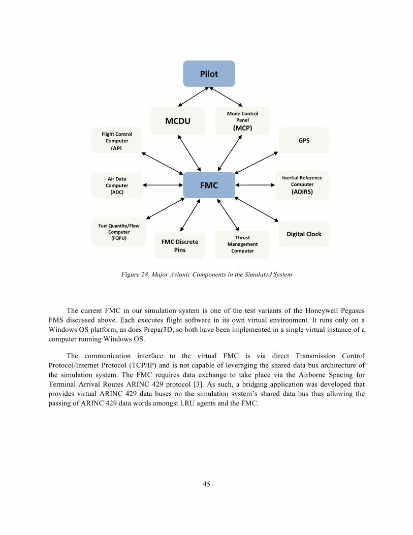
45

Figure 28. Major Avionic Components in the Simulated System

The current FMC in our simulation system is one of the test variants of the Honeywell Pegasus FMS discussed above. Each executes flight software in its own virtual environment. It runs only on a Windows OS platform, as does Prepar3D, so both have been implemented in a single virtual instance of a computer running Windows OS.

The communication interface to the virtual FMC is via direct Transmission Control Protocol/Internet Protocol (TCP/IP) and is not capable of leveraging the shared data bus architecture of the simulation system. The FMC requires data exchange to take place via the Airborne Spacing for Terminal Arrival Routes ARINC 429 protocol [3]. As such, a bridging application was developed that provides virtual ARINC 429 data buses on the simulation system’s shared data bus thus allowing the passing of ARINC 429 data words amongst LRU agents and the FMC.

FMC

Flight Control Computer (AP)

Air Data Computer (ADC)

Fuel Quantity/Flow Computer (FQPU) FMC Discrete

Pins

Digital Clock

Inertial Reference Computer (ADIRS)

GPS

MCDU Mode Control

Panel (MCP)

Pilot

Thrust Management Computer (TMC)

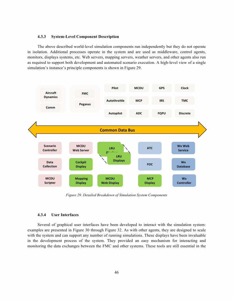
46

4.3.3 System-Level Component Description

The above described world-level simulation components run independently but they do not operate in isolation. Additional processes operate in the system and are used as middleware, control agents, monitors, displays systems, etc. Web servers, mapping servers, weather servers, and other agents also run as required to support both development and automated scenario execution. A high-level view of a single simulation’s instance’s principle components is shown in Figure 29.

Figure 29. Detailed Breakdown of Simulation System Components

4.3.4 User Interfaces

Several of graphical user interfaces have been developed to interact with the simulation system: examples are presented in Figure 30 through Figure 32. As with other agents, they are designed to scale with the system and can support any number of running simulations. These displays have been invaluable in the development process of the system. They provided an easy mechanism for interacting and monitoring the data exchanges between the FMC and other systems. These tools are still essential in the

Autopilot ADC FQPU Discrete

Clock

IRS

GPS MCDU

MCP

Pilot

TMC Autothrottle

FMC

Pegasus

Aircraft Dynamics

Comm

Scenario Controller

Data Collection

MCDU Web Server

Cockpit Display

Mapping Display

LRU Displays LRU Displays

LRU Displays

Wx Web Service

Wx Database

Wx Controller

MCDU Web Display

MCP Display

MCDU Scripter

ATC

FOC

Common Data Bus

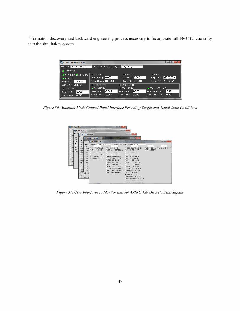
47

information discovery and backward engineering process necessary to incorporate full FMC functionality into the simulation system.

Figure 30. Autopilot Mode Control Panel Interface Providing Target and Actual State Conditions

Figure 31. User Interfaces to Monitor and Set ARINC 429 Discrete Data Signals

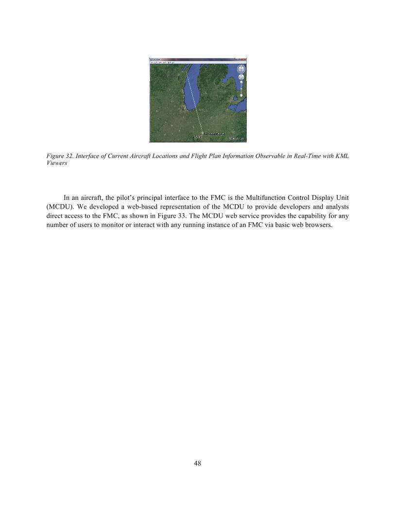
48

Figure 32. Interface of Current Aircraft Locations and Flight Plan Information Observable in Real-Time with KML Viewers

In an aircraft, the pilot’s principal interface to the FMC is the Multifunction Control Display Unit (MCDU). We developed a web-based representation of the MCDU to provide developers and analysts direct access to the FMC, as shown in Figure 33. The MCDU web service provides the capability for any number of users to monitor or interact with any running instance of an FMC via basic web browsers.

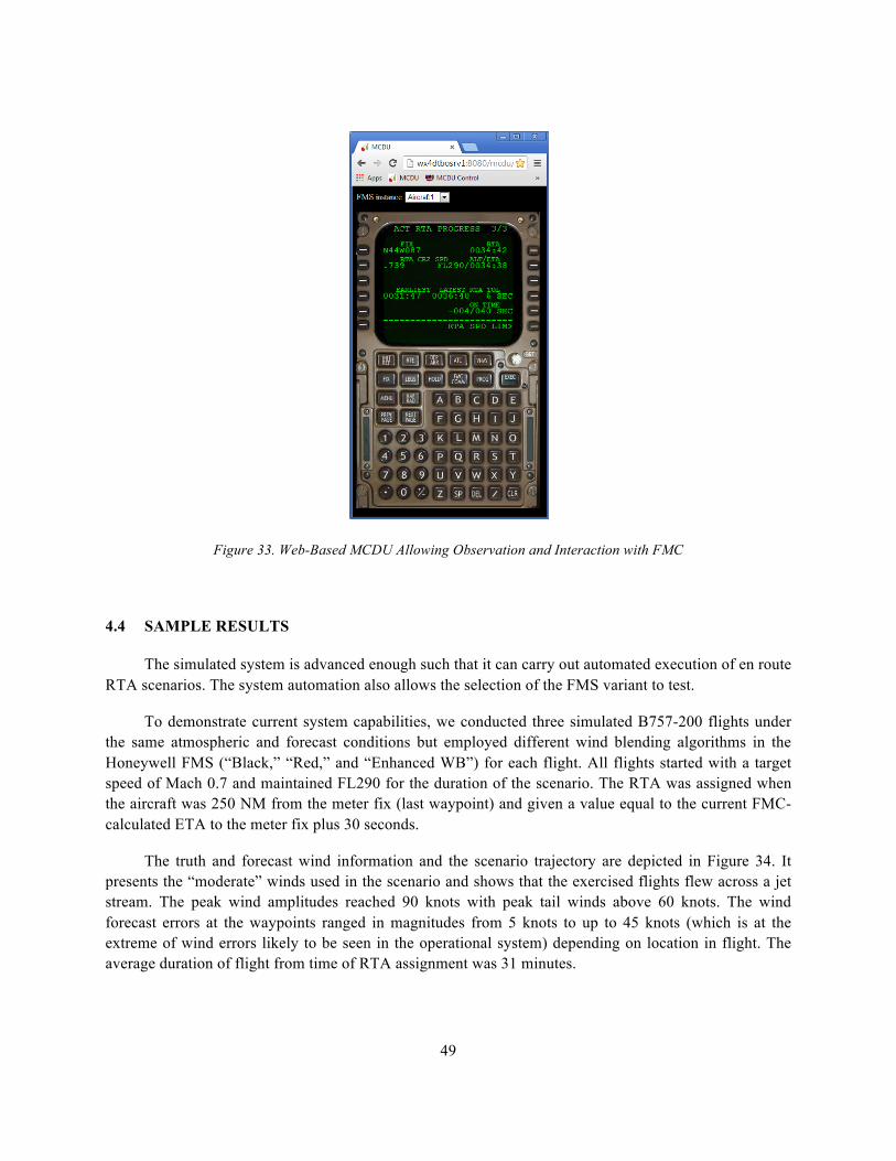
49

Figure 33. Web-Based MCDU Allowing Observation and Interaction with FMC

4.4 SAMPLE RESULTS

The simulated system is advanced enough such that it can carry out automated execution of en route RTA scenarios. The system automation also allows the selection of the FMS variant to test.

To demonstrate current system capabilities, we conducted three simulated B757-200 flights under the same atmospheric and forecast conditions but employed different wind blending algorithms in the Honeywell FMS (“Black,” “Red,” and “Enhanced WB”) for each flight. All flights started with a target speed of Mach 0.7 and maintained FL290 for the duration of the scenario. The RTA was assigned when the aircraft was 250 NM from the meter fix (last waypoint) and given a value equal to the current FMC-calculated ETA to the meter fix plus 30 seconds.

The truth and forecast wind information and the scenario trajectory are depicted in Figure 34. It presents the “moderate” winds used in the scenario and shows that the exercised flights flew across a jet stream. The peak wind amplitudes reached 90 knots with peak tail winds above 60 knots. The wind forecast errors at the waypoints ranged in magnitudes from 5 knots to up to 45 knots (which is at the extreme of wind errors likely to be seen in the operational system) depending on location in flight. The average duration of flight from time of RTA assignment was 31 minutes.

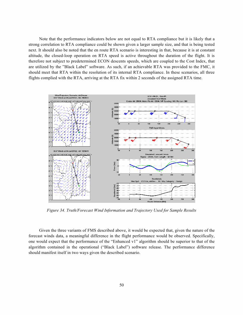
50

Note that the performance indicators below are not equal to RTA compliance but it is likely that a strong correlation to RTA compliance could be shown given a larger sample size, and that is being tested next. It should also be noted that the en route RTA scenario is interesting in that, because it is at constant altitude, the closed-loop operation on RTA speed is active throughout the duration of the flight. It is therefore not subject to predetermined ECON descents speeds, which are coupled to the Cost Index, that are utilized by the ”Black Label” software. As such, if an achievable RTA was provided to the FMC, it should meet that RTA within the resolution of its internal RTA compliance. In these scenarios, all three flights complied with the RTA, arriving at the RTA fix within 2 seconds of the assigned RTA time.

Figure 34. Truth/Forecast Wind Information and Trajectory Used for Sample Results

Given the three variants of FMS described above, it would be expected that, given the nature of the forecast winds data, a meaningful difference in the flight performance would be observed. Specifically, one would expect that the performance of the “Enhanced v1” algorithm should be superior to that of the algorithm contained in the operational (“Black Label”) software release. The performance difference should manifest itself in two ways given the described scenario.

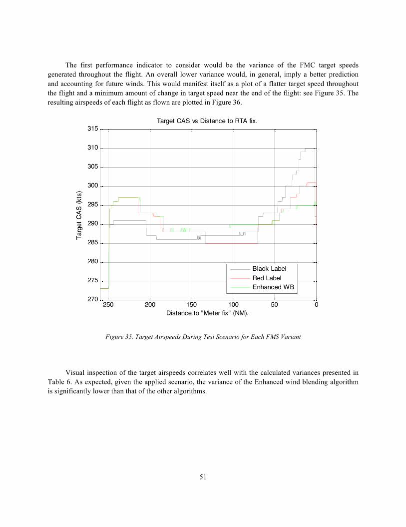
51

The first performance indicator to consider would be the variance of the FMC target speeds generated throughout the flight. An overall lower variance would, in general, imply a better prediction and accounting for future winds. This would manifest itself as a plot of a flatter target speed throughout the flight and a minimum amount of change in target speed near the end of the flight: see Figure 35. The resulting airspeeds of each flight as flown are plotted in Figure 36.

Figure 35. Target Airspeeds During Test Scenario for Each FMS Variant

Visual inspection of the target airspeeds correlates well with the calculated variances presented in Table 6. As expected, given the applied scenario, the variance of the Enhanced wind blending algorithm is significantly lower than that of the other algorithms.

050100150200250270

275

280

285

290

295

300

305

310

315

Distance to "Meter fix" (NM).

Targ

et C

AS (k

ts)

Target CAS vs Distance to RTA fix.

Black LabelRed LabelEnhanced WB

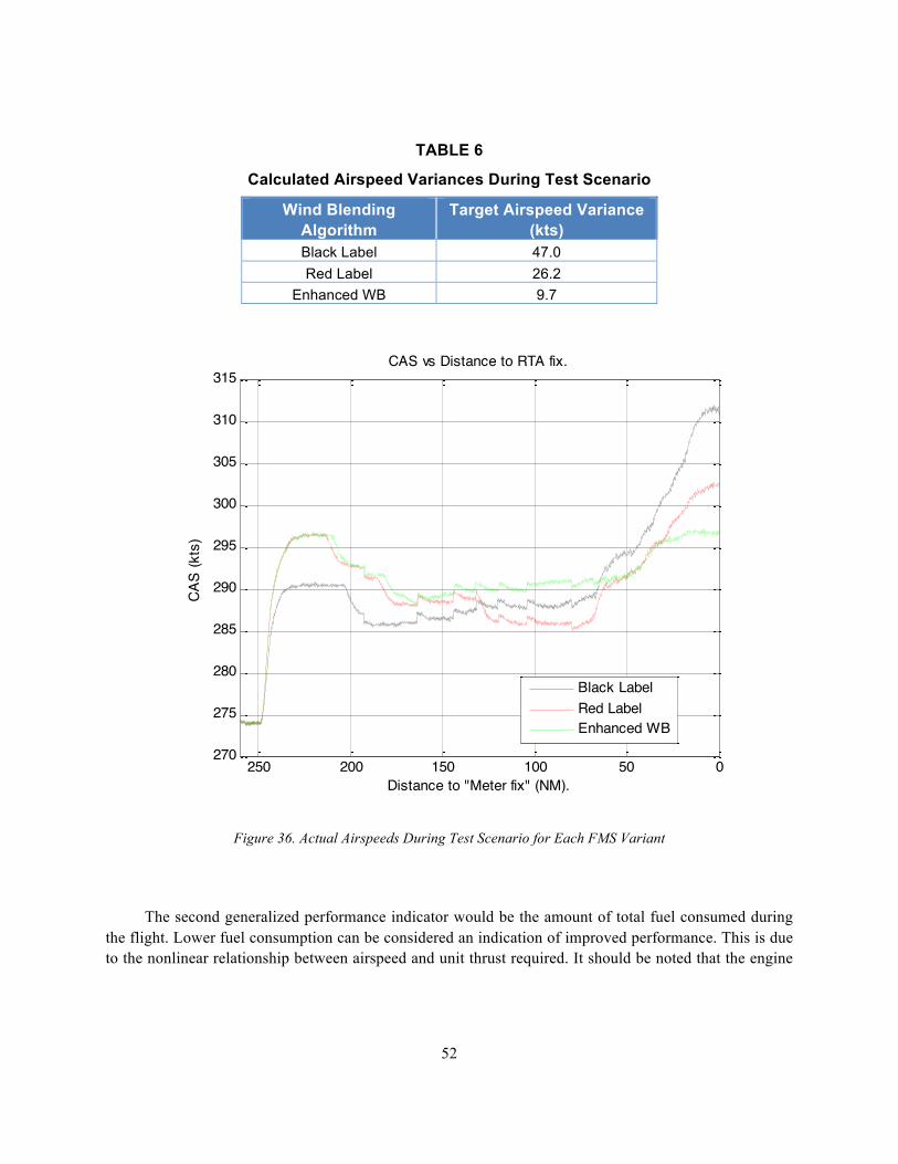
52

TABLE 6

Calculated Airspeed Variances During Test Scenario

Wind Blending Algorithm

Target Airspeed Variance (kts)

Black Label 47.0 Red Label 26.2

Enhanced WB 9.7

Figure 36. Actual Airspeeds During Test Scenario for Each FMS Variant

The second generalized performance indicator would be the amount of total fuel consumed during the flight. Lower fuel consumption can be considered an indication of improved performance. This is due to the nonlinear relationship between airspeed and unit thrust required. It should be noted that the engine

050100150200250270

275

280

285

290

295

300

305

310

315

Distance to "Meter fix" (NM).

CAS

(kts

)

CAS vs Distance to RTA fix.

Black LabelRed LabelEnhanced WB

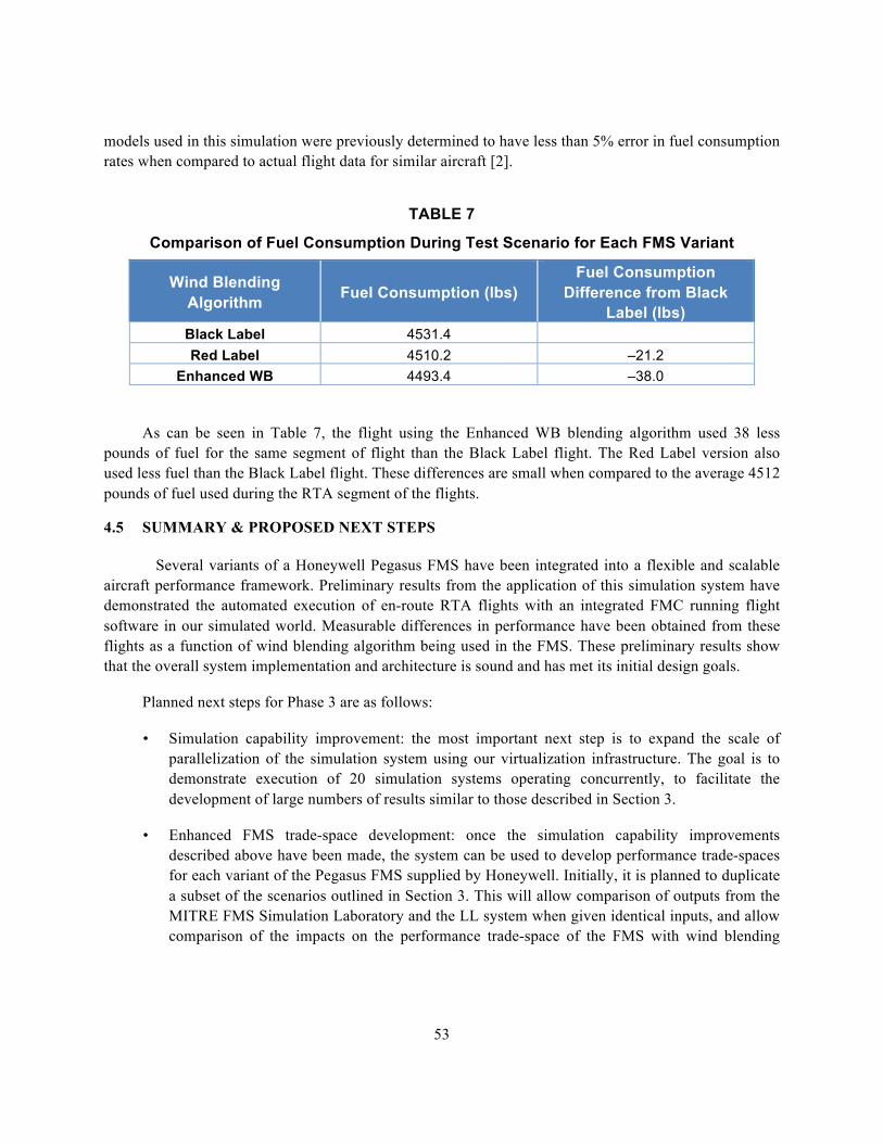
53

models used in this simulation were previously determined to have less than 5% error in fuel consumption rates when compared to actual flight data for similar aircraft [2].

TABLE 7

Comparison of Fuel Consumption During Test Scenario for Each FMS Variant

Wind Blending Algorithm Fuel Consumption (lbs)

Fuel Consumption Difference from Black

Label (lbs) Black Label 4531.4 Red Label 4510.2 –21.2

Enhanced WB 4493.4 –38.0

As can be seen in Table 7, the flight using the Enhanced WB blending algorithm used 38 less pounds of fuel for the same segment of flight than the Black Label flight. The Red Label version also used less fuel than the Black Label flight. These differences are small when compared to the average 4512 pounds of fuel used during the RTA segment of the flights.


Several variants of a Honeywell Pegasus FMS have been integrated into a flexible and scalable aircraft performance framework. Preliminary results from the application of this simulation system have demonstrated the automated execution of en-route RTA flights with an integrated FMC running flight software in our simulated world. Measurable differences in performance have been obtained from these flights as a function of wind blending algorithm being used in the FMS. These preliminary results show that the overall system implementation and architecture is sound and has met its initial design goals.

Planned next steps for Phase 3 are as follows:

• Simulation capability improvement: the most important next step is to expand the scale of parallelization of the simulation system using our virtualization infrastructure. The goal is to demonstrate execution of 20 simulation systems operating concurrently, to facilitate the development of large numbers of results similar to those described in Section 3.

• Enhanced FMS trade-space development: once the simulation capability improvements described above have been made, the system can be used to develop performance trade-spaces for each variant of the Pegasus FMS supplied by Honeywell. Initially, it is planned to duplicate a subset of the scenarios outlined in Section 3. This will allow comparison of outputs from the MITRE FMS Simulation Laboratory and the LL system when given identical inputs, and allow comparison of the impacts on the performance trade-space of the FMS with wind blending

54

enhancements. In parallel, it is recommended to explore new scenarios that explicitly test the response of the different FMS variants.

• At present only one new FMS variant with wind blending algorithm enhancements has been provided and exercised. The simulation framework is now to a point that other FMS enhancements could also be tested (e.g., to the interpolation algorithms for winds between waypoints, number of wind entry altitudes at each waypoint). These will be discussed with the sponsor to establish priority level.

4.6 REFERENCES

[1] Honeywell Aerospace, “B757/767 Pegasus Flight Management System Pilot’s Guide,” February 2002.


[3] Honeywell International Inc., “FMC_ICD_111025.doc,” 10/25/2011.

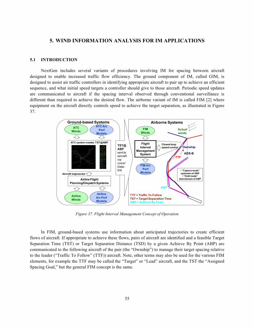
55

5. WIND INFORMATION ANALYSIS FOR IM APPLICATIONS

5.1 INTRODUCTION

NextGen includes several variants of procedures involving IM for spacing between aircraft designed to enable increased traffic flow efficiency. The ground component of IM, called GIM, is designed to assist air traffic controllers in identifying appropriate aircraft to pair up to achieve an efficient sequence, and what initial speed targets a controller should give to those aircraft. Periodic speed updates are communicated to aircraft if the spacing interval observed through conventional surveillance is different than required to achieve the desired flow. The airborne variant of IM is called FIM [2] where equipment on the aircraft directly controls speed to achieve the target separation, as illustrated in Figure 37.

Figure 37. Flight Interval Management Concept of Operation

In FIM, ground-based systems use information about anticipated trajectories to create efficient flows of aircraft. If appropriate to achieve these flows, pairs of aircraft are identified and a feasible Target Separation Time (TST) or Target Separation Distance (TSD) by a given Achieve By Point (ABP) are communicated to the following aircraft of the pair (the “Ownship”) to manage their target spacing relative to the leader (“Traffic To Follow” (TTF)) aircraft. Note, other terms may also be used for the various FIM elements, for example the TTF may be called the “Target” or “Lead” aircraft, and the TST the “Assigned Spacing Goal,” but the general FIM concept is the same.

Actualwinds

Ground-based Systems Airborne SystemsATC

WindsATC A/c

Perf Models

FIMWinds

FIM A/c Perf

Models

FlightInterval

Management System

TTF

Ownship

ABP

TTF = Traffic To FollowTST = Target Separation TimeABP = Achieve By Point

Closed-loopspeed control

ADS-B

• “Capture mode” upstream of ABP

• “Hold mode” downstream of ABP

ATC system creates TST@ABP

AirlineWinds

AirlineA/c Perf Models

Airline Flight Planning/Dispatch Systems

TST@ABPsent to aircraft via voice/ Data-link

Aircraft trajectories

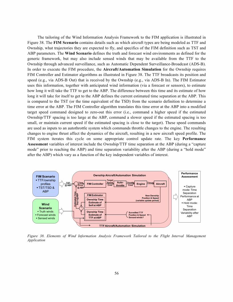
56

The tailoring of the Wind Information Analysis Framework to the FIM application is illustrated in Figure 38. The FIM Scenario contains details such as which aircraft types are being modeled as TTF and Ownship, what trajectories they are expected to fly, and specifics of the FIM definition such as TST and ABP parameters. The Wind Scenario defines the truth and forecast wind environments as defined for the generic framework, but may also include sensed winds that may be available from the TTF to the Ownship through advanced surveillance, such as Automatic Dependent Surveillance-Broadcast (ADS-B). In order to execute the FIM procedure, the Aircraft/Automation Simulation for the Ownship requires FIM Controller and Estimator algorithms as illustrated in Figure 38. The TTF broadcasts its position and speed (e.g., via ADS-B Out) that is received by the Ownship (e.g., via ADS-B In). The FIM Estimator uses this information, together with anticipated wind information (via a forecast or sensors), to estimate how long it will take the TTF to get to the ABP. The difference between this time and its estimate of how long it will take for itself to get to the ABP defines the current estimated time separation at the ABP. This is compared to the TST (or the time equivalent of the TSD) from the scenario definition to determine a time error at the ABP. The FIM Controller algorithm translates this time error at the ABP into a modified target speed command designed to zero-out this error (i.e., command a higher speed if the estimated Ownship/TTF spacing is too large at the ABP, command a slower speed if the estimated spacing is too small, or maintain current speed if the estimated spacing is close to the target). These speed commands are used as inputs to an autothrottle system which commands throttle changes to the engine. The resulting changes to engine thrust affect the dynamics of the aircraft, resulting in a new aircraft speed profile. The FIM system iterates this cycle on some appropriate control update rate. The key Performance Assessment variables of interest include the Ownship/TTF time separation at the ABP (during a “capture mode” prior to reaching the ABP) and time separation variability after the ABP (during a “hold mode” after the ABP) which vary as a function of the key independent variables of interest.

Figure 38. Elements of Wind Information Analysis Framework Tailored to the Flight Interval Management Application

Ownship Aircraft/Automation Simulation

FIM ControllerTimeError

@ ABP

Ownship Time Estimate of Self at ABP

Ownship Time Estimate of TTF at ABP

FIM Estimator

TST@ ABP

Estim

ated

Tim

eSe

p’n@

ABP

TargetSpeedCmd

Auto-throttle

ThrottleCmd Engine

New OwnshipPosition & Speed

(variable update period)

AircraftThrust

Surveilled TTFPosition & SpeedSensed winds?


§ Capture mode: Time Separation

Performance at ABP

§ Hold mode: Time

Separation Variability after

ABP

Wind Scenario

§ Truth winds§ Forecast winds§ Sensed winds

FIM Scenario§ TTF/ownship

profiles§ TST/TSD &

ABP

TTF Aircraft/Automation Simulation

+-

+-

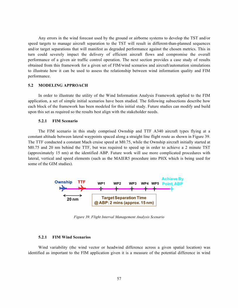
57

Any errors in the wind forecast used by the ground or airborne systems to develop the TST and/or speed targets to manage aircraft separation to the TST will result in different-than-planned sequences and/or target separations that will manifest as degraded performance against the chosen metrics. This in turn could severely impact the delivery of efficient aircraft flows and compromise the overall performance of a given air traffic control operation. The next section provides a case study of results obtained from this framework for a given set of FIM/wind scenarios and aircraft/automation simulations to illustrate how it can be used to assess the relationship between wind information quality and FIM performance.

5.2 MODELING APPROACH

In order to illustrate the utility of the Wind Information Analysis Framework applied to the FIM application, a set of simple initial scenarios have been studied. The following subsections describe how each block of the framework has been modeled for this initial study. Future studies can modify and build upon this set as required so the results best align with the stakeholder needs.

5.2.1 FIM Scenario

The FIM scenario in this study comprised Ownship and TTF A340 aircraft types flying at a constant altitude between lateral waypoints spaced along a straight line flight route as shown in Figure 39. The TTF conducted a constant Mach cruise speed at M0.75, while the Ownship aircraft initially started at M0.75 and 20 nm behind the TTF, but was required to speed up in order to achieve a 2 minute TST (approximately 15 nm) at the identified ABP. Future work will use more complicated procedures with lateral, vertical and speed elements (such as the MAIER5 procedure into PHX which is being used for some of the GIM studies).

Figure 39. Flight Interval Management Analysis Scenario

5.2.1 FIM Wind Scenarios

Wind variability (the wind vector or headwind difference across a given spatial location) was identified as important to the FIM application given it is a measure of the potential difference in wind

TTFAchieve ByPoint, ABPOwnship

Target Separation Time@ ABP: 2 mins (approx. 15 nm)

WP1 WP2 WP3 WP4 WP5

20 nm

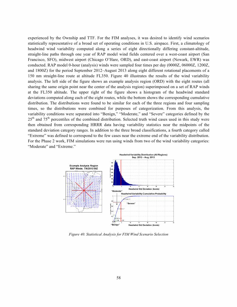
58

experienced by the Ownship and TTF. For the FIM analyses, it was desired to identify wind scenarios statistically representative of a broad set of operating conditions in U.S. airspace. First, a climatology of headwind wind variability computed along a series of eight directionally differing constant-altitude, straight-line paths through one year of RAP model wind fields centered over a west-coast airport (San Francisco, SFO), midwest airport (Chicago O’Hare, ORD), and east-coast airport (Newark, EWR) was conducted. RAP model 0-hour (analysis) winds were sampled four times per day (0000Z, 06000Z, 1200Z, and 1800Z) for the period September 2012–August 2013 along eight different rotational placements of a 150 nm straight-line route at altitude FL350. Figure 40 illustrates the results of the wind variability analysis. The left side of the figure shows an example analysis region (ORD) with the eight routes (all sharing the same origin point near the center of the analysis region) superimposed on a set of RAP winds at the FL350 altitude. The upper right of the figure shows a histogram of the headwind standard deviations computed along each of the eight routes, while the bottom shows the corresponding cumulative distribution. The distributions were found to be similar for each of the three regions and four sampling times, so the distributions were combined for purposes of categorization. From this analysis, the variability conditions were separated into “Benign,” “Moderate,” and “Severe” categories defined by the 25th and 75th percentiles of the combined distribution. Selected truth wind cases used in this study were then obtained from corresponding HRRR data having variability statistics near the midpoints of the standard deviation category ranges. In addition to the three broad classifications, a fourth category called “Extreme” was defined to correspond to the few cases near the extreme end of the variability distribution. For the Phase 2 work, FIM simulations were run using winds from two of the wind variability categories: “Moderate” and “Extreme.”

Figure 40. Statistical Analysis for FIM Wind Scenario Selection

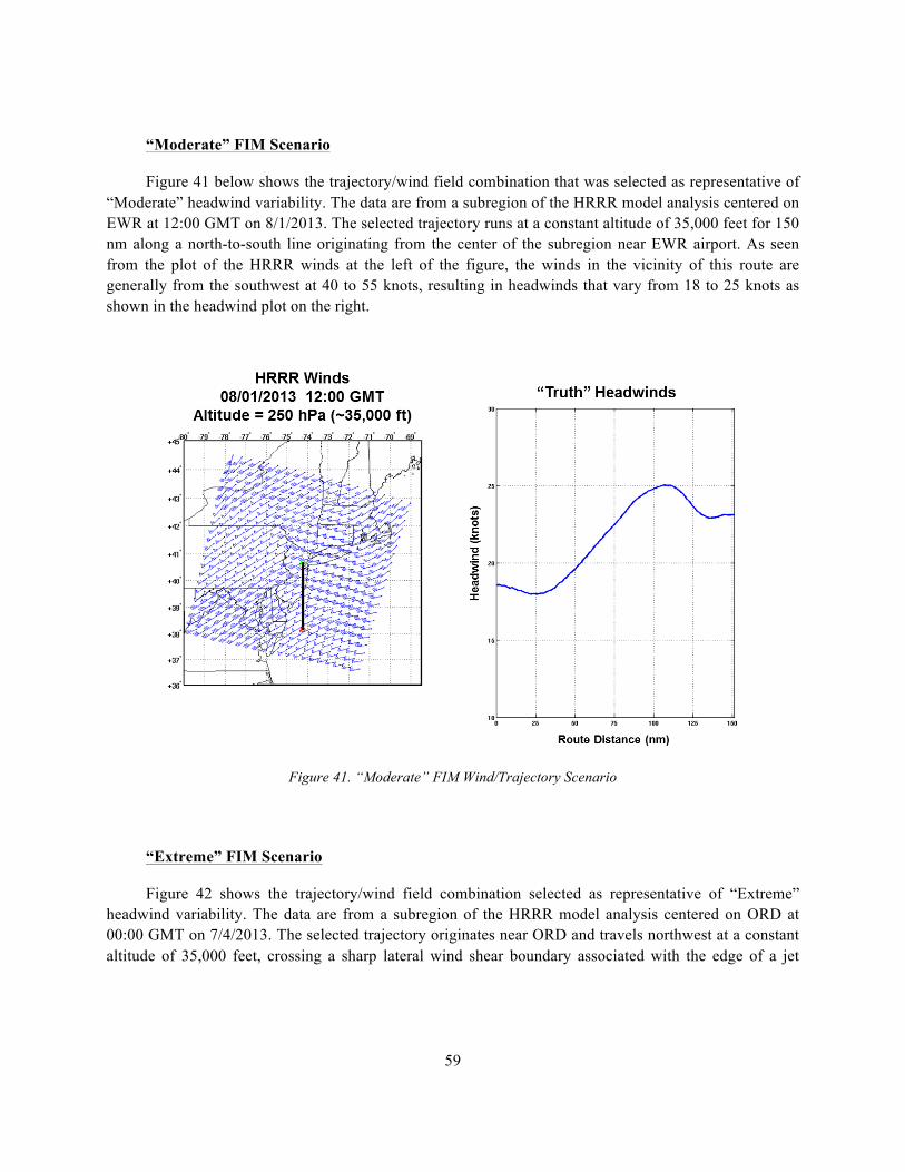
59

“Moderate” FIM Scenario

Figure 41 below shows the trajectory/wind field combination that was selected as representative of “Moderate” headwind variability. The data are from a subregion of the HRRR model analysis centered on EWR at 12:00 GMT on 8/1/2013. The selected trajectory runs at a constant altitude of 35,000 feet for 150 nm along a north-to-south line originating from the center of the subregion near EWR airport. As seen from the plot of the HRRR winds at the left of the figure, the winds in the vicinity of this route are generally from the southwest at 40 to 55 knots, resulting in headwinds that vary from 18 to 25 knots as shown in the headwind plot on the right.

Figure 41. “Moderate” FIM Wind/Trajectory Scenario

“Extreme” FIM Scenario

Figure 42 shows the trajectory/wind field combination selected as representative of “Extreme” headwind variability. The data are from a subregion of the HRRR model analysis centered on ORD at 00:00 GMT on 7/4/2013. The selected trajectory originates near ORD and travels northwest at a constant altitude of 35,000 feet, crossing a sharp lateral wind shear boundary associated with the edge of a jet

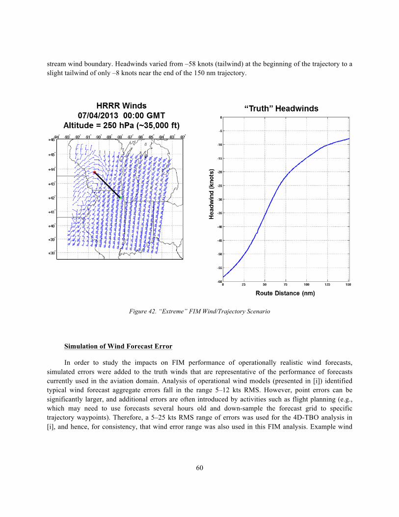
60

stream wind boundary. Headwinds varied from –58 knots (tailwind) at the beginning of the trajectory to a slight tailwind of only –8 knots near the end of the 150 nm trajectory.

Figure 42. “Extreme” FIM Wind/Trajectory Scenario

Simulation of Wind Forecast Error

In order to study the impacts on FIM performance of operationally realistic wind forecasts, simulated errors were added to the truth winds that are representative of the performance of forecasts currently used in the aviation domain. Analysis of operational wind models (presented in [i]) identified typical wind forecast aggregate errors fall in the range 5–12 kts RMS. However, point errors can be significantly larger, and additional errors are often introduced by activities such as flight planning (e.g., which may need to use forecasts several hours old and down-sample the forecast grid to specific trajectory waypoints). Therefore, a 5–25 kts RMS range of errors was used for the 4D-TBO analysis in [i], and hence, for consistency, that wind error range was also used in this FIM analysis. Example wind

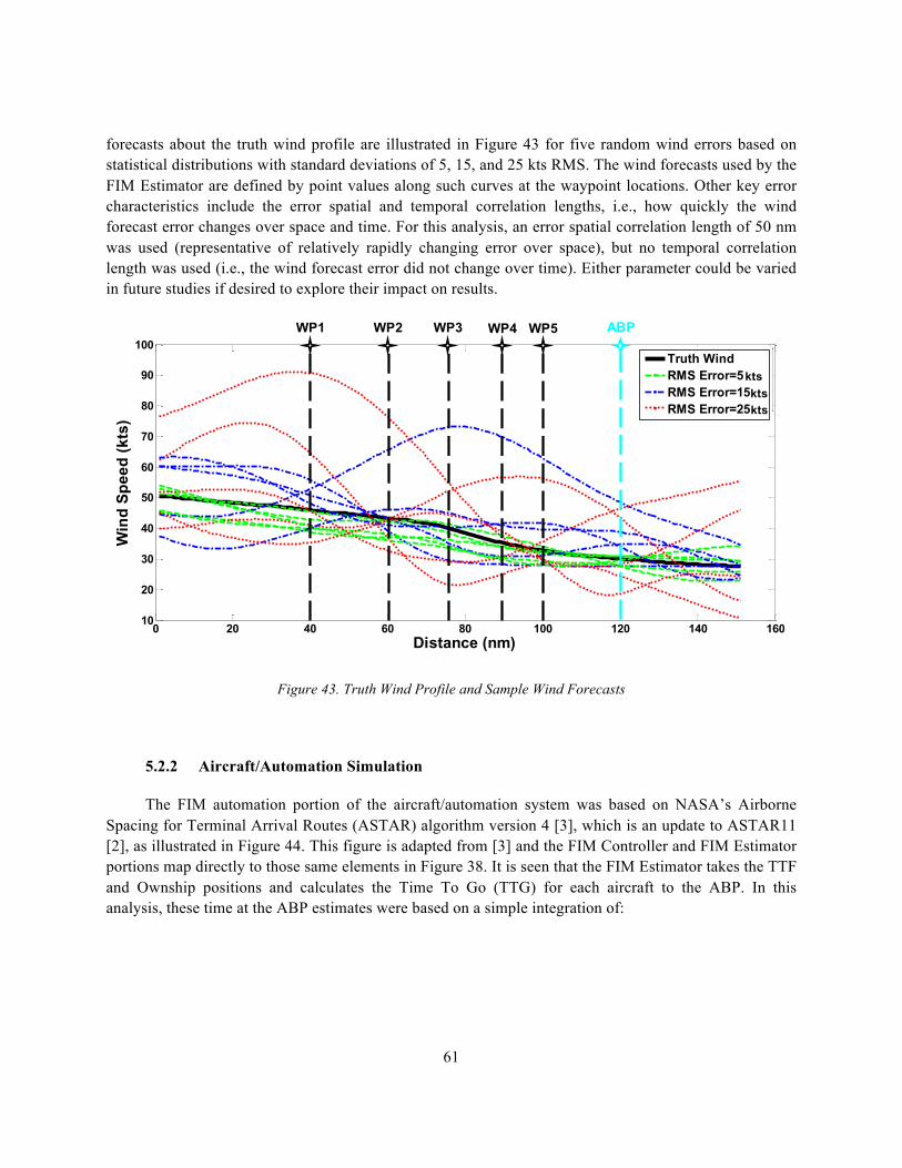
61

forecasts about the truth wind profile are illustrated in Figure 43 for five random wind errors based on statistical distributions with standard deviations of 5, 15, and 25 kts RMS. The wind forecasts used by the FIM Estimator are defined by point values along such curves at the waypoint locations. Other key error characteristics include the error spatial and temporal correlation lengths, i.e., how quickly the wind forecast error changes over space and time. For this analysis, an error spatial correlation length of 50 nm was used (representative of relatively rapidly changing error over space), but no temporal correlation length was used (i.e., the wind forecast error did not change over time). Either parameter could be varied in future studies if desired to explore their impact on results.

Figure 43. Truth Wind Profile and Sample Wind Forecasts

5.2.2 Aircraft/Automation Simulation

The FIM automation portion of the aircraft/automation system was based on NASA’s Airborne Spacing for Terminal Arrival Routes (ASTAR) algorithm version 4 [3], which is an update to ASTAR11 [2], as illustrated in Figure 44. This figure is adapted from [3] and the FIM Controller and FIM Estimator portions map directly to those same elements in Figure 38. It is seen that the FIM Estimator takes the TTF and Ownship positions and calculates the Time To Go (TTG) for each aircraft to the ABP. In this analysis, these time at the ABP estimates were based on a simple integration of:

0 20 40 60 80 100 120 140 16010

20

30

40

50

60

70

80

90

100

Win

d Sp

eed

(kts

)

Distance (nm)

Truth WindRMS Error=5RMS Error=15RMS Error=25

ABPWP1 WP2 WP3 WP4 WP5

0 20 40 60 80 100 120 140 16010

20

30

40

50

60

70

80

90

100

Win

d Sp

eed

(kts

)

Distance (nm)

Truth WindRMS Error=5RMS Error=15RMS Error=25

ktsktskts

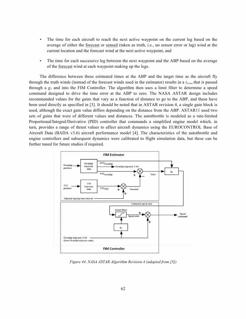
62

• The time for each aircraft to reach the next active waypoint on the current leg based on the average of either the forecast or sensed (taken as truth, i.e., no sensor error or lag) wind at the current location and the forecast wind at the next active waypoint, and

• The time for each successive leg between the next waypoint and the ABP based on the average of the forecast wind at each waypoint making up the legs.

The difference between these estimated times at the ABP and the target time as the aircraft fly through the truth winds (instead of the forecast winds used in the estimator) results in a terror that is passed through a g1 and into the FIM Controller. The algorithm then uses a limit filter to determine a speed command designed to drive the time error at the ABP to zero. The NASA ASTAR design includes recommended values for the gains that vary as a function of distance to go to the ABP, and these have been used directly as specified in [3]. It should be noted that in ASTAR revision 4, a single gain block is used, although the exact gain value differs depending on the distance from the ABP. ASTAR11 used two sets of gains that were of different values and distances. The autothrottle is modeled as a rate-limited Proportional/Integral/Derivative (PID) controller that commands a simplified engine model which, in turn, provides a range of thrust values to affect aircraft dynamics using the EUROCONTROL Base of Aircraft Data (BADA v3.6) aircraft performance model [4]. The characteristics of the autothrottle and engine controllers and subsequent dynamics were calibrated to flight simulation data, but these can be further tuned for future studies if required.

Figure 44. NASA ASTAR Algorithm Revision 4 (adapted from [3])

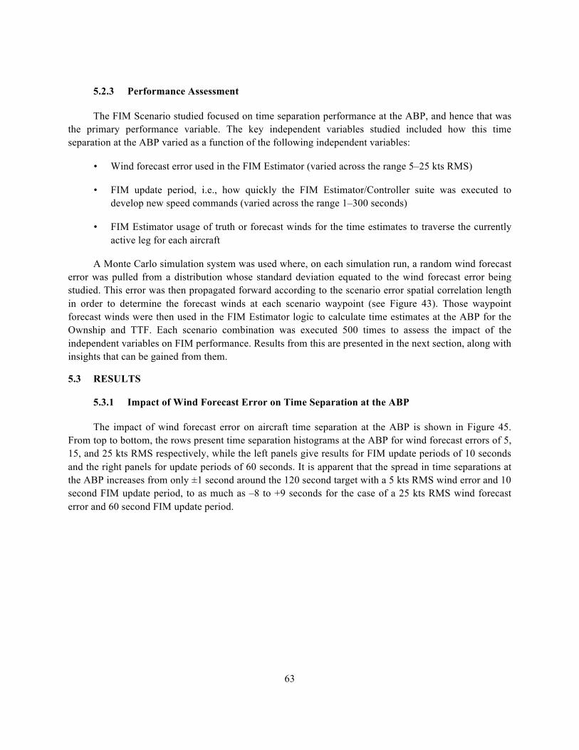
63

5.2.3 Performance Assessment

The FIM Scenario studied focused on time separation performance at the ABP, and hence that was the primary performance variable. The key independent variables studied included how this time separation at the ABP varied as a function of the following independent variables:

• Wind forecast error used in the FIM Estimator (varied across the range 5–25 kts RMS)

• FIM update period, i.e., how quickly the FIM Estimator/Controller suite was executed to develop new speed commands (varied across the range 1–300 seconds)

• FIM Estimator usage of truth or forecast winds for the time estimates to traverse the currently active leg for each aircraft

A Monte Carlo simulation system was used where, on each simulation run, a random wind forecast error was pulled from a distribution whose standard deviation equated to the wind forecast error being studied. This error was then propagated forward according to the scenario error spatial correlation length in order to determine the forecast winds at each scenario waypoint (see Figure 43). Those waypoint forecast winds were then used in the FIM Estimator logic to calculate time estimates at the ABP for the Ownship and TTF. Each scenario combination was executed 500 times to assess the impact of the independent variables on FIM performance. Results from this are presented in the next section, along with insights that can be gained from them.

5.3 RESULTS

5.3.1 Impact of Wind Forecast Error on Time Separation at the ABP

The impact of wind forecast error on aircraft time separation at the ABP is shown in Figure 45. From top to bottom, the rows present time separation histograms at the ABP for wind forecast errors of 5, 15, and 25 kts RMS respectively, while the left panels give results for FIM update periods of 10 seconds and the right panels for update periods of 60 seconds. It is apparent that the spread in time separations at the ABP increases from only ±1 second around the 120 second target with a 5 kts RMS wind error and 10 second FIM update period, to as much as –8 to +9 seconds for the case of a 25 kts RMS wind forecast error and 60 second FIM update period.

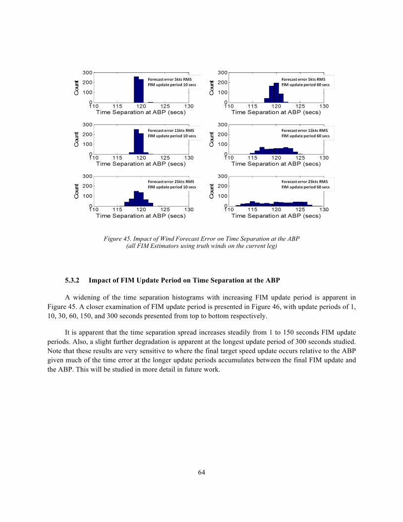
64

Figure 45. Impact of Wind Forecast Error on Time Separation at the ABP (all FIM Estimators using truth winds on the current leg)

5.3.2 Impact of FIM Update Period on Time Separation at the ABP

A widening of the time separation histograms with increasing FIM update period is apparent in Figure 45. A closer examination of FIM update period is presented in Figure 46, with update periods of 1, 10, 30, 60, 150, and 300 seconds presented from top to bottom respectively.

It is apparent that the time separation spread increases steadily from 1 to 150 seconds FIM update periods. Also, a slight further degradation is apparent at the longest update period of 300 seconds studied. Note that these results are very sensitive to where the final target speed update occurs relative to the ABP given much of the time error at the longer update periods accumulates between the final FIM update and the ABP. This will be studied in more detail in future work.

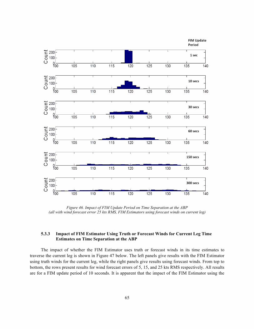
65

Figure 46. Impact of FIM Update Period on Time Separation at the ABP (all with wind forecast error 25 kts RMS, FIM Estimators using forecast winds on current leg)

5.3.3 Impact of FIM Estimator Using Truth or Forecast Winds for Current Leg Time Estimates on Time Separation at the ABP

The impact of whether the FIM Estimator uses truth or forecast winds in its time estimates to traverse the current leg is shown in Figure 47 below. The left panels give results with the FIM Estimator using truth winds for the current leg, while the right panels give results using forecast winds. From top to bottom, the rows present results for wind forecast errors of 5, 15, and 25 kts RMS respectively. All results are for a FIM update period of 10 seconds. It is apparent that the impact of the FIM Estimator using the

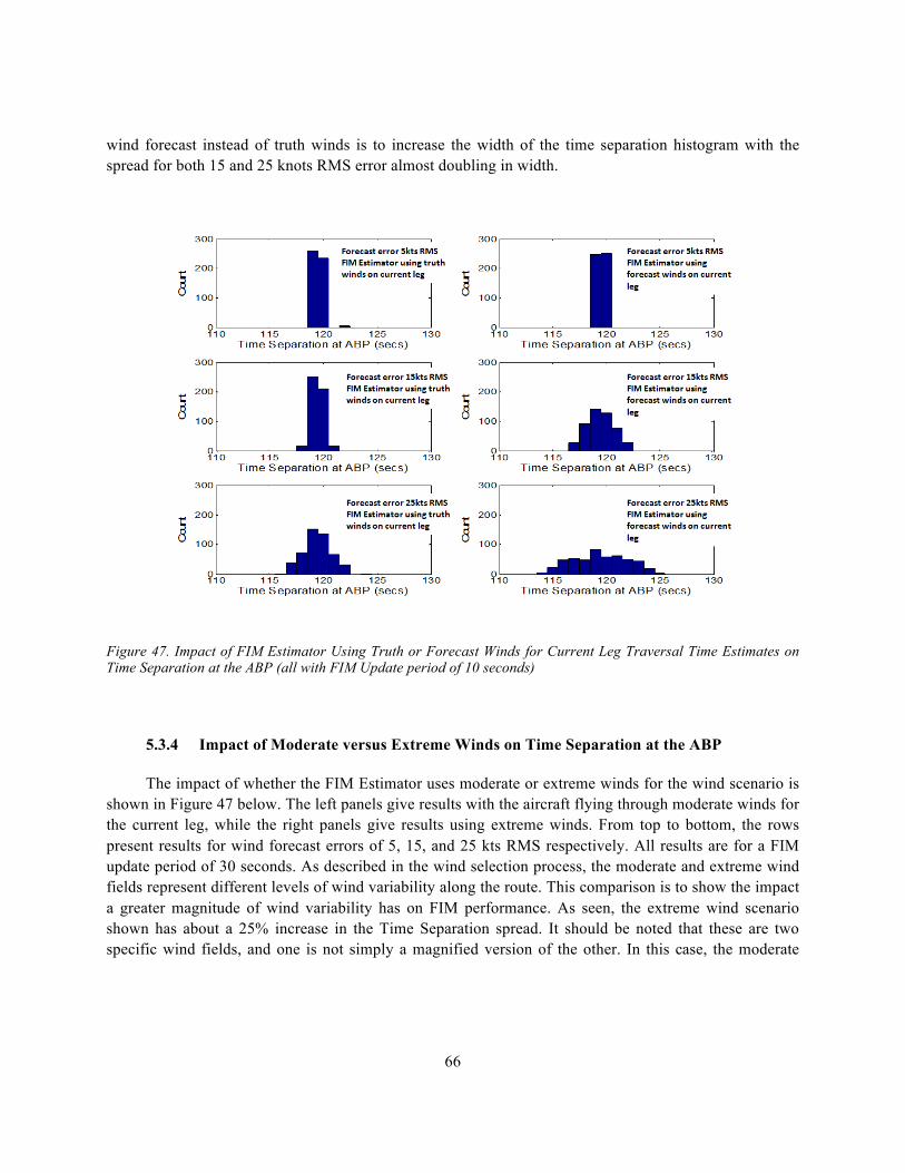
66

wind forecast instead of truth winds is to increase the width of the time separation histogram with the spread for both 15 and 25 knots RMS error almost doubling in width.

Figure 47. Impact of FIM Estimator Using Truth or Forecast Winds for Current Leg Traversal Time Estimates on Time Separation at the ABP (all with FIM Update period of 10 seconds)

5.3.4 Impact of Moderate versus Extreme Winds on Time Separation at the ABP

The impact of whether the FIM Estimator uses moderate or extreme winds for the wind scenario is shown in Figure 47 below. The left panels give results with the aircraft flying through moderate winds for the current leg, while the right panels give results using extreme winds. From top to bottom, the rows present results for wind forecast errors of 5, 15, and 25 kts RMS respectively. All results are for a FIM update period of 30 seconds. As described in the wind selection process, the moderate and extreme wind fields represent different levels of wind variability along the route. This comparison is to show the impact a greater magnitude of wind variability has on FIM performance. As seen, the extreme wind scenario shown has about a 25% increase in the Time Separation spread. It should be noted that these are two specific wind fields, and one is not simply a magnified version of the other. In this case, the moderate

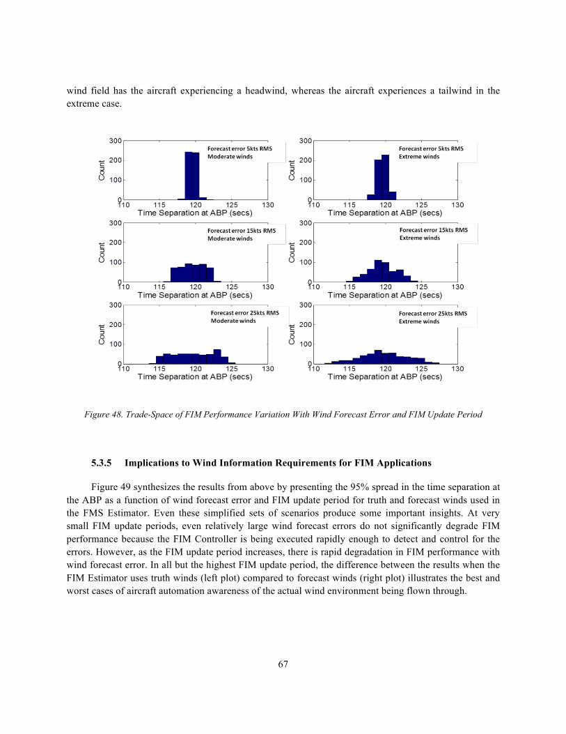
67

wind field has the aircraft experiencing a headwind, whereas the aircraft experiences a tailwind in the extreme case.

Figure 48. Trade-Space of FIM Performance Variation With Wind Forecast Error and FIM Update Period

5.3.5 Implications to Wind Information Requirements for FIM Applications

Figure 49 synthesizes the results from above by presenting the 95% spread in the time separation at the ABP as a function of wind forecast error and FIM update period for truth and forecast winds used in the FMS Estimator. Even these simplified sets of scenarios produce some important insights. At very small FIM update periods, even relatively large wind forecast errors do not significantly degrade FIM performance because the FIM Controller is being executed rapidly enough to detect and control for the errors. However, as the FIM update period increases, there is rapid degradation in FIM performance with wind forecast error. In all but the highest FIM update period, the difference between the results when the FIM Estimator uses truth winds (left plot) compared to forecast winds (right plot) illustrates the best and worst cases of aircraft automation awareness of the actual wind environment being flown through.

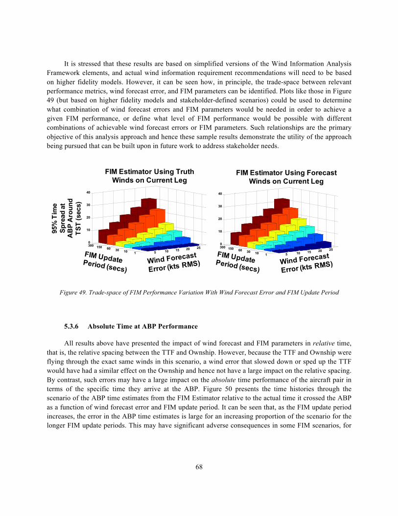
68

It is stressed that these results are based on simplified versions of the Wind Information Analysis Framework elements, and actual wind information requirement recommendations will need to be based on higher fidelity models. However, it can be seen how, in principle, the trade-space between relevant performance metrics, wind forecast error, and FIM parameters can be identified. Plots like those in Figure 49 (but based on higher fidelity models and stakeholder-defined scenarios) could be used to determine what combination of wind forecast errors and FIM parameters would be needed in order to achieve a given FIM performance, or define what level of FIM performance would be possible with different combinations of achievable wind forecast errors or FIM parameters. Such relationships are the primary objective of this analysis approach and hence these sample results demonstrate the utility of the approach being pursued that can be built upon in future work to address stakeholder needs.

Figure 49. Trade-space of FIM Performance Variation With Wind Forecast Error and FIM Update Period

5.3.6 Absolute Time at ABP Performance

All results above have presented the impact of wind forecast and FIM parameters in relative time, that is, the relative spacing between the TTF and Ownship. However, because the TTF and Ownship were flying through the exact same winds in this scenario, a wind error that slowed down or sped up the TTF would have had a similar effect on the Ownship and hence not have a large impact on the relative spacing. By contrast, such errors may have a large impact on the absolute time performance of the aircraft pair in terms of the specific time they arrive at the ABP. Figure 50 presents the time histories through the scenario of the ABP time estimates from the FIM Estimator relative to the actual time it crossed the ABP as a function of wind forecast error and FIM update period. It can be seen that, as the FIM update period increases, the error in the ABP time estimates is large for an increasing proportion of the scenario for the longer FIM update periods. This may have significant adverse consequences in some FIM scenarios, for

FIM Estimator Using Truth Winds on Current Leg

FIM Estimator Using Forecast Winds on Current Leg

95%

Tim

eSp

read

atA

BP

Aro

und

TST

(sec

s)

1103060150300

5 10 15 20 250

10

20

30

40

1103060150300

5 10 15 20 250

10

20

30

40

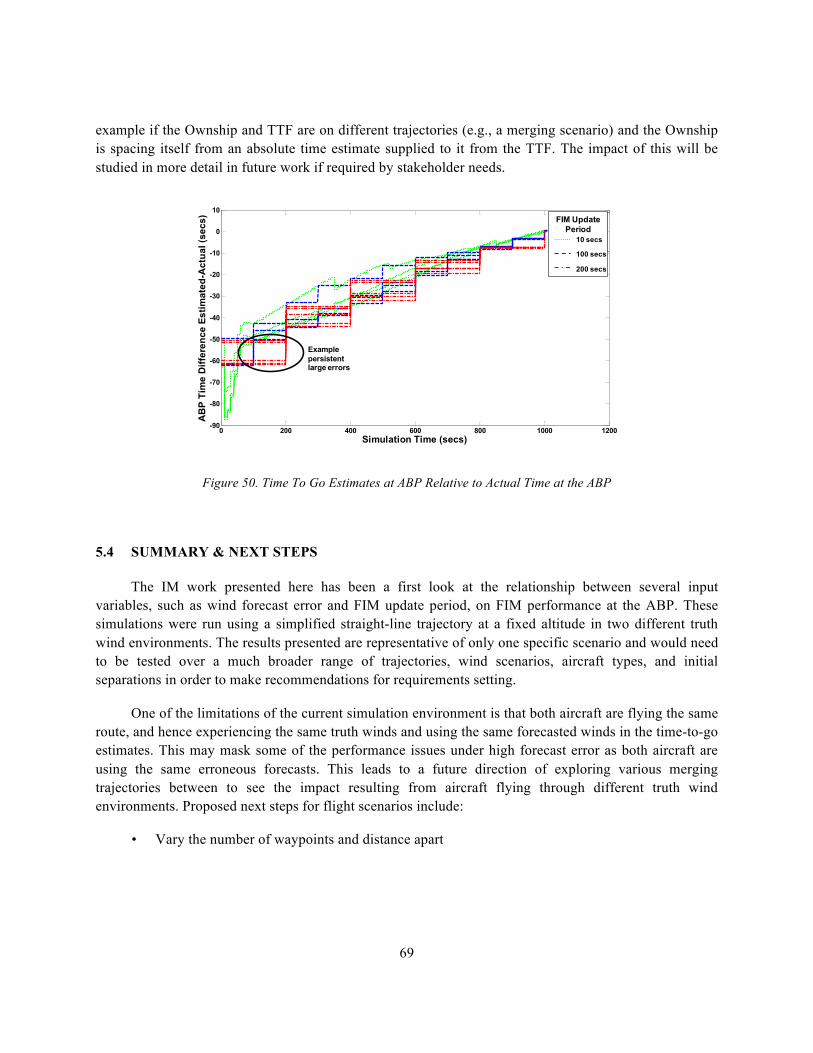
69

example if the Ownship and TTF are on different trajectories (e.g., a merging scenario) and the Ownship is spacing itself from an absolute time estimate supplied to it from the TTF. The impact of this will be studied in more detail in future work if required by stakeholder needs.

Figure 50. Time To Go Estimates at ABP Relative to Actual Time at the ABP

5.4 SUMMARY & NEXT STEPS

The IM work presented here has been a first look at the relationship between several input variables, such as wind forecast error and FIM update period, on FIM performance at the ABP. These simulations were run using a simplified straight-line trajectory at a fixed altitude in two different truth wind environments. The results presented are representative of only one specific scenario and would need to be tested over a much broader range of trajectories, wind scenarios, aircraft types, and initial separations in order to make recommendations for requirements setting.

One of the limitations of the current simulation environment is that both aircraft are flying the same route, and hence experiencing the same truth winds and using the same forecasted winds in the time-to-go estimates. This may mask some of the performance issues under high forecast error as both aircraft are using the same erroneous forecasts. This leads to a future direction of exploring various merging trajectories between to see the impact resulting from aircraft flying through different truth wind environments. Proposed next steps for flight scenarios include:

• Vary the number of waypoints and distance apart

0 200 400 600 800 1000 1200-90

-80

-70

-60

-50

-40

-30

-20

-10

0

10

Simulation Time (secs)

AB

P Ti

me

Diff

eren

ce E

stim

ated

-Act

ual (

secs

)

FIM=10sFIM=30sFIM=100sFIM=200s

FIM Update Period

10 secs

100 secs

200 secs

Examplepersistentlarge errors

70

• Run merging scenarios, with aircraft merging at the ABP from angles of 0, 45, 90, 135, and 180 degrees

For the merging scenarios, another factor to be studied is the wind assumptions the Ownship uses to predict the TTF’s arrival at the ABP. The Ownship may or may not have a forecast for the TTF trajectory, and if not would need to make assumptions about the winds on that route. Proposed merging wind assumptions include:

• Full knowledge of waypoints and forecast for the TTF

• Assume zero wind for the entire route

• Project ownship forecast winds onto TTF trajectory

Another next step would be testing new wind environments. In the current study, a moderate and extreme wind environment were tested. These were classified based on the variability across the entire trajectory. However, the impact of the wind variability would likely be different depending on how quickly the winds change and also where along the trajectory an area of high wind variability is located. It is likely that the same change in wind speeds would have more of an impact on FIM performance the closer it occurs to the ABP. Proposed next steps for wind scenarios include:

• Run existing scenario on a range of headwind speeds and variabilities

• On 0-degree merge, vary location of high variability as function of distance to ABP

• Run merging scenarios with different levels of variation between the truth winds for the two trajectories

5.5 REFERENCES

[1] Glina, Y., Troxel, S., Reynolds, T., and McPartland, M., “Wind Information Requirements to Support Four Dimensional Trajectory-Based Operations,” 12th AIAA Aviation Technology, Integration, and Operations (ATIO) Conference, 17–19 September 2012, Indianapolis, Indiana, Paper AIAA 2012-5702.

[2] RTCA, “Safety, Performance and Interoperability Requirements Document For Airborne Spacing – Flight Deck Interval Management (ASPA FIM),” DO-328, Washington, DC, 2011.

[3] Abbott, T. S., “An Overview of a Trajectory-Based Solution for En Route and Terminal Area Self-Spacing,” NASA/CR-2012-217786, 2012.

[4] EUROCONTROL, Base of Aircraft Data, Version 3.6, 2004.

71

6. SUMMARY

Many future air transportation system paradigms require access to high quality wind information. The primary objective of this work is to quantify the relationship between wind information quality and benefits delivery under these future ATC applications. This information will be of high value to stakeholders, for example, in terms of determining wind forecasting performance and automation technology requirements in ground and airborne systems to achieve NextGen goals. In the first phase of the work, a Wind Information Analysis Framework has been developed that is designed to be flexible and scalable to explore wind information needs across a broad range of applications. It was applied to a realistic 4D-TBO scenario with simplified versions of the framework elements under a challenging wind environment with representative wind error models to provide proof-of-concept of the utility of the framework.

Phase 2 activities have built upon the Phase 1 foundation by using refined and expanded applications of the Wind Information Analysis Framework. The report has documented the refined wind information metrics and wind scenario selection process applicable to a broader range of NextGen applications, with particular focus on 4D-TBO and IM. Expanded and refined studies of 4D-TBO applications with current FMSs (with MITRE collaboration) have identified the main drivers of 4D-TBO performance, and how these can be used to establish more focused trade-spaces from which wind information quality requirements can be established, as well as identifying combinations of operational variables (wind data content, accuracy, update rate, etc.) that can achieve the required level of wind information. The report has described the expansion of the 4D-TBO study using incremental enhancements possible in future FMSs (with Honeywell collaboration), specifically in the area of wind blending algorithms to quantify performance improvement potential from near-term avionics refinements. Finally, the adaptability of the Wind Information Analysis Framework has been demonstrated by using it to identify initial wind information needs for a variety of sample IM applications.

Proposed next steps in Phase 3 activities have been highlighted throughout each section of the report, with the general objective of addressing specific stakeholder requirements, for example, in the areas of:

• Determining wind information implications of different 4D-TBO and IM performance targets through refined trade-space development

• Operational implications of the resulting wind information quality levels required to support those performance levels in terms of concept of operation and datalink requirements


73

GLOSSARY

4D-TBO Four-Dimensional Trajectory Based Operations ABP Achieve By Point ADS-B Automatic Dependent Surveillance-Broadcast ARINC Aeronautical Radio Inc. ASTAR Airborne Spacing for Terminal Arrival Routes ATC Air Traffic Control BADA Base of Aircraft Data CG Center-of-Gravity ConOps Concept of Operation EAGUL5 Phoenix Airport Approach Procedure ECON Economy ETA Estimated Time of Arrival EWR New York Newark Airport FAF Final Approach Fix FIM Flight Interval Management FMC Flight Management Computer FMS Flight Management System FOC Flight Operations Center GE General Electric GIM Ground Interval Management HRRR High Resolution Rapid Refresh IM Interval Management kts Knots LL Lincoln Laboratory LRUs Line-Replaceable Units MCDU Multifunction Control Display Unit NARR North America Regional Reanalysis NextGen Next Generation Air Transportation System nm Nautical Mile ORD Chicago O’Hare Airport PHX Phoenix International Airport PID Proportional/Integral/Derivative RAP Rapid Refresh RMS Root Means Square RMSE Root Mean Square Error RTA Required Time of Arrival RUC Rapid Update Cycle

74

SFO San Francisco Airport SLIDR Waypoint along EAGUL5 Phoenix Airport Approach Procedure STARs Standard Terminal Arrival Routes TCP/IP Transmission Control Protocol/Internet Protocol TOD Top-Of-Descent TSD Target Separation Distance TST Target Separation Time TTF Traffic To Follow TTG Time To Go

Documents

Wind Information Requirements for NextGen Applications ... · 2 Wind Information Analysis Framework 2! 3 4D-TBO Challenging Wind Environments 6! 4 Wind Metric and ATC/Wind Scenario