Embed Size (px)
Citation preview

What is the Economic Explanation of Size and BooktoMarket Effects in
the Mexican Stock Market Returns?
Abstract
The technique employed by Fama and French (1993) is used to perform a time
series analysis to examine whether the CAPM is the adequate model to give the
economic explanation for the roles of size and booktomarket value in the
Mexican stock market returns or whether a MultiFactor Pricing Model gives a
better explication. The evidence shows that the business conditions are
important to identify the adequate risk factor. We found that the average returns
are explained by different risk factors in different time periods.

2
Comments welcome
XI Congreso Internacional de la
Academia de Ciencias Administrativas
(ACACIA)
What is the Economic Explanation of Size and BooktoMarket Effects in
the Mexican Stock Market Returns?
Tema: Finanzas y Economía.
Jorge Enrique Velarde Chapa 1 and
Ana Dolores Espinoza Borbón 2
Instituto Tecnológico y de Estudios Superiores de Monterrey. Campus Guadalajara
Av. General Ramón Corona 2514 Col. Nuevo México. Zapopan, Jalisco, México.
Tel: (33) 36693000 Ext. 2255 y 2279 Email: [email protected] y [email protected]
Zapopan, Jalisco, México. 19 de enero de 2007.
1 Professor Jorge Enrique Velarde Chapa, Research and Consulting Center, Instituto Tecnológico y de Estudios Super iores de Monterrey, Campus Guadalajara. 2 Research Assistant Ana Dolores Espinoza Borbón, Research and Consulting Center, Instituto Tecnológico y de Estudios Super iores de Monterrey, Campus Guadalajara.

3
Abstract
The technique employed by Fama and French (1993) is used to perform a time
series analysis to examine whether the CAPM is the adequate model to give the
economic explanation for the roles of size and booktomarket value in the
Mexican stock market returns or whether a MultiFactor Pricing Model gives a
better explication. The evidence shows that the business conditions are
important to identify the adequate risk factor. We found that the average returns
are explained by different risk factors in different time periods.
Key Words: Arbitrage, Capital Asset Pricing Model, MultiFactor Pricing Model,
Size, Book to Market, Anomalies, Mexican Stock Market.
JEL: G12, G15

4
I. INTRODUCTION
The tradeoff between risk factors and stock returns has been an issue of
several investigations in developed countries. The Capital Asset Pricing Model
(CAPM) and MultiFactor Pricing Model are some of the main models used to
explain this relationship.
The origin of the CAPM is attributed to four authors. Markowitz (1952)
proposed that investors select their portfolio maximizing its expected return and
minimizing its variance. Sharpe (1964) argued that equilibrium exists in a simple
linear relation between the expected return and the return’s standard deviation.
He emphasized the necessity of obtaining an equilibrium condition in the capital
markets for an efficient combination of risky assets. Lintner (1965) developed
this equilibrium by creating an original algebraic framework. Black (1972)
developed a less restrictive version of the CAPM that does not depend on the
existence of a riskfree asset; unlike the version of SharpeLintner, which
depends on the existence of a riskfree asset.
It is true that the CAPM has been a topic of several empirical research
works. However, in this model some patterns inside stock returns are not
explained and only one risk factor is considered. Authors mention these patterns
without explaining CAPM anomalies, where the most common are the size (a
stock’s price times shares outstanding) and booktomarket value.
A negative correlation between size and stock returns was documented by
Banz (1981). He finds that market equity, size adds to the explanation of the
crosssection of average returns provided by market Betas. Average returns on

5
small stocks are too high given their market beta estimates, and average returns
on large stocks are too low. The correlation between booktomarket value and
stock returns was documented by Stattman (1980) and Rosemberg, Reid and
Lanstein (1992), finding that average returns on US stocks are positively related
to the booktomarket value, and by Chan, Hamao and Lakonishok (1991), who
found that this characteristic also has a strong role in explaining the cross
section of average returns on Japanese stocks.
The MultiFactor Pricing Model was proposed as an alternative to the
CAPM in order to include more than one risk factor explaining the expected
returns. Merton (1973) and Ross (1976) were pioneers in this area, with the
following empirical studies as the main research trying to test these models3:
Chen, Roll and Ross (1986) explored a set of economic variables such as
the systematic influence on stock markets returns and examined their influence
on asset pricing. Chen, Chan and Heish (1985) analyzed the possibility of a
MultiFactor Pricing Model as an explanation of the firm size effect. Clare and
Thomas (1994) showed empirical evidence of the pricing of macroeconomic risk
factors on the British Stock Market using different portfolio ordering techniques,
such as betas and size.
He and Ng (1994) explored whether size and booktomarket value are
proxies for macroeconomic risk factors or measures of stock risk exposure to
distress. Fama and French (1992) investigated the roles of market beta, size,
earningstoprice ratio (EP), leverage and booktomarket value in average stock
3 The Intertemporal CAPM was developed by Merton (1973) and the Arbitrage Pricing Theory by Ross (1976)

6
returns. Fama and French (1993) identified common risk factors in stocks and
bond returns, considering additional variables like size, booktomarket value and
EP value. Lakonishok, Shleifer and Vishny (1994) suggested that the high
returns associated with high booktomarket values are generated by investors
who incorrectly extrapolate the past earnings growth rates of firms.
Take in consideration the argument that the inconsistency in the CAPM
could be the result of the crosssection differences in stock returns are related
with some stock characteristics, the objective in this empirical research is to
perform a time series analysis to examine whether the CAPM is the adequate
model to give the economic explanation for the roles of size and booktomarket
value in the Mexican stock market returns or whether a MultiFactor Pricing
Model gives a better explication.
The remainder of the paper is organized as follows. Section II, describes
the period of study and the data base used. Section III, the effect of size and
booktomarket value in the stock market returns is presented. Section IV
present the economic explication for the size booktomarket portfolios. Finally,
the conclusions are discussed in Section V.
II. DATA DESCRIPTION
A. PERIOD OF STUDY
The database of stock prices and risk factors variables covers a period
spanning from January 1987 to December 2001. Furthermore, with the purpose
of testing whether the results are substantially affected by structural changes, the
entire sample will be divided into four subperiods. The subperiods from January

7
1987 to December 1994 and from January 1995 to December 2001 will evaluate
the economic and financial shock which took place during December 1994 and
the effect that the Mexican economy became more open since NAFTA was
implemented in 1994. The subperiods from January 1987 to May 1989 and from
June 1989 to December 2001 will evaluate the impact of the Mexican financial
liberalization, which started in May 1989 (Levine and Zervos 1994).
B. STOCK MARKET VARIABLES
During the 19872001 period, 176 firms issued stocks in the Mexican
Stock Market. Nevertheless there are 66 other stocks trading in the market as a
result of 54 firms issuing multiple classes of the same stock, which will be also
included in my study in order to minimize survivorship bias. The total sample in
this study will consist of 242 individual stock price series.
The sample contains 180 months. On average, the stocks contain 108
observations available for each monthly series, with a maximum of 180
observations and a minimum of 5 observations.
In order to reduce survivorship bias and delisting bias to be included in
the sample, a stock must have traded in the examined interval at least once over
the sample period, even though some stocks have minimal trading or are only
traded for a short period, the stock that exits in the examined interval will also be
considered.
The returns are computed in terms of continuously compounded monthly
growth rates according to the following equation:

8
( ) ( ) [ ] 1 ln ln 1 − − = − t t t P P R (1)
The reasons for using continuously compounded returns instead of
percentage returns is due to the fact that log returns reduce the bias in returns
induced by bid/ask spread and price discreteness (Mucklow 1994), the
heteroskedasticity found in most stock return series is reduced and the
compound returns often exhibit a higher degree of normality than percentage
returns (Vaihekoski 2000).
Infosel Inversionista, Finsat, Economatica and the Emerging Market Data
Base (EMDB) of the International Financial Corporation will supply the database
of monthly adjusted closing prices.
C. RISK FACTORS VARIABLES
Table I lists the definitions of the risk factors. Panel A describes the basic
series that will not be used as risk factors. Panel B describes the derived series
obtained from the basic series, which will be used as risk factors.
[Insert Table I]
The National Institute of Statistics, Geography and Computing (INEGI)
and the Mexican Central Bank (BANXICO) will supply the local risk factors and
international risk factors. All variables will be measured in terms of continuously
compounded monthly growth rates, except for the expected and unexpected

9
inflation, SMB and HML portfolios, exchange rate, liquidity proxy, momentum
mimicking portfolio, political risk, term structure and default risk.
SMB (small minus big size) and HML (high minus low B/M)
Portfolios. Keeping in mind that Banz (1981) found that stocks of smaller firms
that have a lack of information are to be perceived by investors as riskier
investments, and Fama and French’s (1992) arguments that booktomarket
value is related with earnings which influences a strong positive relation between
average return and booktomarket value, I formed two portfolios to mimic the
premium that could result from these two firm characteristics, thus explaining
whether there is a relationship with the expected returns.
In June of each year, starting at 1987 through 2001, all individual stocks
are ranked on size, breaking the stocks into two equally sized groups, small firms
(S) and big firms (B). Furthermore, at the end of each December I sorted S and
B groups by booktomarket value, breaking each two groups in three bookto
market groups, low (L), medium (M) and high (H).
Considering the intersections of two size groups and three booktomarket
groups, I constructed six equally weighed portfolios: SL, SM, SH, BL, BM and
BH. For example, the SL portfolio includes firms in the small size group that are
also in the low booktomarket group, the BH portfolio includes firms in the big
size group that are also in the high booktomarket group, and so on.
These six portfolios are used to construct the SMB and HML variables.
SMB is the difference between the average of the returns on the three small size
stock portfolios (SL+SM+SH)/3 and the three big size stock portfolios
(BL+BM+BH)/3. This difference tries to measure the risk factor in returns related

10
to size effect. HML is the difference between the average of the returns on the
two high booktomarket stock portfolios (SH+BH)/2 and the two low bookto
market stock portfolios (SL+BL)/2. This difference allows capturing the risk factor
in returns related to booktomarket effect.
Exchange Rate (EX). The volatility of the exchange rate is an important
factor risk emphasized by Bailey and Chung (1995) and Choi, Hikari and
Takezawa (1998) in Emerging Markets, since the exchange rate is significantly
volatile for the exporting firms and cash flows are adversely affected by the
appreciation in the real value of the domestic currency, which affect the stock
price negatively. We obtained the change in exchange rate like shows in
equation 2 with the objective to measure the effect on the returns.
EXMt = log[EXt] – log[EXt1] (2)
Political Risk (POLITIC). Firms that are particularly sensitive to economic
conditions may be exposed to political risks due to their broad impact on the
economy, which, similar to the exchange rate, is reflected directly in their cash
flow and, therefore, on stock prices. We are going to measure the political risk as
the monthly return spread between a dollar bond issued by the Mexican
government and the TBILLS.
POLITIC = SCETES/EXM – TBILLN (3)

11
This measure assumes the Bailey and Chung’s (1995) hypothesis that credit
risk and political risk are positively correlated. When political risk declines, the
probability of sovereign default decreases and Mexican dollar bonds experience
price appreciation relative to US Treasury debt. Thus, POLITIC increases as
political risk decreases.
Default Risk (DEF). Since the unexpected change in interest rates and the
economic conditions that change the likelihood of default are risk factors that
have an influence on stock returns, Chen, Roll and Ross (1986) use variables
like DEF to help explain these risks.
We calculate DEF is obtained as the difference between longterm corporate
bonds and the longterm government bond. In Mexico there is no historical
information about the longterm corporate bond. For this reason, we used the
commercial paper issued by corporations as a proxy for this bond.
D. DATA DESCRIPTIVE STATISTICS
In Table II, the correlation coefficients among the risk factors are shown.
In general, the correlations are not large except between risk factors that have a
close relation. Risk factors such as DEF, TBILLR and EXM are influenced by
inflation in their calculation, which increases their correlation between 0.803 and
0.284. Another group that has a high correlation corresponds to series that were
calculated using similar variables. The stock market variables as SMB, HML and
EMR present a correlation between 0.230 to 0.992.
[Insert Table II]

12
Summary of descriptive statistics of risk factors are reported in Table III
Except for U.S. real interest rate (TBILLR), according to the JarqueBera
statistic, all series have a normal distribution. In relation to TBILLR, the normal
distribution graph is adequate and kurtosis is higher than three, concluding that
this variable could hasve a tendency to behave like a normal distribution,
although normality is rejected by the JarqueBera statistic.
[Insert Table III]
Another important point is that HML and SMB means are negative,
inverse to the size and booktomarket effects. This could mean that the mimic
premium of these characteristics is not measured. However, the real reason is
due to financial market liberalization, a more open economy and the Mexican
financial crisis of December 1994.
Table IV supports these reasons. For example, Panel A illustrates how the
financial market liberalization starting in May 1989 affects the premium of the
size and booktomarket mimicking portfolios. These effects are documented by
Cervantes (1999) and Patro and Wald (2001). In the Mexican stock market for
the period from 1989 to 1998, Cervantes (1999) found a negative average return
of 1.08 for SMB and 3.54 for HML. Patro and Wald (2001) found before the
start of the financial liberalization positive average returns of 5.26 and 10.78 in
SMB and HML respectively and negative average returns of 1.58 and –1.67
after the start of the liberalization. They argued that when markets are
liberalized, securities that were originally subject to the national risk price are re
priced according to the world market price of risk, which caused those stocks

13
returns to increase during liberalization and decline afterwards, because the
firms’ cash flow is now dispersed in the world market while previously it was not.
[Insert Table IV]
Between 1994 and 2003, Mexico has become the country with the largest
network of Free Trade Agreements (FTA’s) in the world. Mexico’s network of
FTA’s comprises 43 countries on three different continents. With the objective to
prove that a more open economy has influence on the HML and SMB means,
Panel B shows the HML and SMB means before 1994 when the Mexico was a
closed economy and the means after 1994 when Mexico opened its economy.
Here is clear that before, both variables are positives in 0.35 and 0.36 and
afterwards they are negatives in 0.44 and 0.65 respectively. This may be a
consequence of the fact that an open economy gives new opportunities for large
firms to compete in a wider world, leaving the small firms in disadvantage
compared to their international competitors. Cervantes (1999) and Francis,
Hasan and Hunter (2001) found similar results, arguing that this differential in
returns between large and small firms is due to the fact that large firms had more
growth than the small firms after Mexico signed the NAFTA in 1994.
Panel B also illustrates that during the Mexican financial crisis of
December 1994, the same phenomenon happened. Before the financial crisis,
the average of HML and SMB are positives in 0.55 and 0.56 respectively. After
the crisis, the average are negatives in 1.01 and 0.79. Patro and Wald (2001)
studied 18 emerging markets, finding that only Mexico has negative SMB

14
premiums due to the Mexican financial crisis of 1994. In other way, Cervantes
(1999) reports also a negative HML premium after a currency crisis, since in
these situations the investors change their preferences for low risk stocks (low
booktomarket) to avoid distressed firms (high booktomarket).
Table V displays the autocorrelation and DickeyFuller stationary test over
the entire sample period, 1987 to 2001. The autocorrelation was tested using the
LjungBox Qstatistics and their pvalues. We found that except for HML all
variables have not autocorrelation.
The absence of autocorrelation in the risk factors is advantageous for the
FM and BJS’s methodologies, since a decrease in the errorinvariables problem
that bias the estimates of the loadings of the stock returns on these risk factors
could bias downward the estimates of the statistical significance.
Similarly, the Dickey Fuller unit root test was carried out to examine the
stationary of each of the risk factors. This test showed that all variables are
stationary, including Dow Jones, HML and Dummy political event, which means
that statistical inferences can be made.
[Insert Table V]
III. SIZE AND BOOK TO MARKET EFFECTS
A joint test is implemented in this section to examine the independent
effect of size and book to market value while controlling the effects of the other
characteristic. The first objective is provide a concrete evidence that size and
booktomarket value better explain the crosssection returns than market beta in

15
the Mexican Stock Market, for next give an economic explanation of size and
booktomarket effects in the average returns.
In the joint test, the crosssection relation between average return and size
and booktomarket value is tested with an average return matrix. This matrix is a
simple picture of the twodimensional variation in average returns that result
when the two size deciles are each subdivided into two portfolios based on
ranked values of booktomarket value for individual stocks. Controlling for size,
booktomarket value capture strong variation in average returns, and controlling
for booktomarket value, size effect capture strong variation in average returns.
The constructions of average return matrix showed in Table VI are based in
sorting the market size and booktomarket value, following the next
methodology.
Given that the Mexican stock market is smaller than the US stock market,
the number of portfolios created on the basis of size and booktomarket value
were four with a minimum of 9 stocks in each portfolio. The portfolio formation
process is similar to Fama and French (1992). In June of each year t, from 1987
to 2001, all individual stocks are ranked in size, breaking the stocks into two
equally size groups, small firms (S) and big firms (B). After this, at the end of
each December t1, I sorted S and B groups by booktomarket value, breaking
each two groups into two booktomarket groups, low (L) and high (H).
Considering the intersections of two size groups and two booktomarket value
groups, we constructed four equally weighed portfolios SL, SH, BL and BH. The
SL portfolio includes firms in the small size group that are also in the low book

16
tomarket value group. BH portfolio includes firms in the big size group that are
also in the high booktomarket value group, and so on.
Table VI shows the average excess returns for the entire period and sub
periods 19871994 and 19952001. In addition to these subperiods, the sub
periods from January 1997 to May 1989 and form June 1989 to December 2001
were included in order to give more robustness to the joint test and more validity
to the results obtained in the original subperiods.
The stock portfolios in the entire sample produce a wide range of average
excess returns, ranging from 0.21 to 0.64 per month. The portfolio behavior
reveals by both, size and booktomarket value, an opposite evidence to the one
found by Fama and French (1992) in the US stock market. For example, the
average excess returns have a positive relation with size. For the low bookto
market value portfolios, the returns increase from 0.34 to 0.64 and for the high
booktomarket from 0.21 to 0.31, whereas the average excess returns have a
negative relation with booktomarket value, for the small size portfolios the
returns decrease from 0.34 to 0.21 and for the big size from 0.64 to 0.31.
[Insert Table VI]
The behavior of average excess returns in the subperiods gives evidence
that the business conditions observed in the Mexican Stock Market are
associated to the reverse behavior found in the entire period.
The subperiods before the financial liberalization and Mexican crisis show
that the behavior of average excess returns are consistent with the evidence
found by Fama and French (1992). The average excess returns decrease with

17
increases in size and increase with increases in booktomarket value. As an
example, before the Mexican crisis, when the size increases in the small book
tomarket portfolios, the average excess returns decrease from 2.11 to 1.80 and
in the high booktomarket portfolios decrease from 2.37 to 2.13. Nevertheless,
when the booktomarket increases in the small size portfolios, the average
excess returns increase form 2.11 to 2.37 and in the big size portfolios increase
from 1.80 to 2.13.
Conversely, the behavior in average excess returns after the financial
liberalization and the Mexican crisis is reversed. As an illustration, after the
Mexican crisis, if the size increases, then average excess return increase from
1.63 to 0.65 and from 2.20 to 1.73 in low and high booktomarket value
portfolios respectively. Nonetheless, if the booktomarket value increases, then
average excess returns decrease from 1.63 to 2.20 and from 0.65 to 1.73 for
the small and big size portfolios respectively. These size and booktomarket
value effects have a similar behavior if the average excess returns before and
after the financial liberalization is observed.
The contrasting behavior of average excess returns in two different
business conditions is not a coincidence. Rather, it is as a consequence of
rational time variation in expected returns such as business returns, investment
opportunities and risk aversion change through time, which causes small firms to
tend to under perform during economic contraction or structural changes. This is
how it behaves after the Mexican crisis and financial liberalization, but
outperforms during periods of economic expansions, which is observed before
the financial deregulation and Mexican crisis (Patro and Wald, 2001).

18
Table VI also shows four portfolios in the entire periods and subperiods
which produce excess returns that show less than 1.645 errors from zero, due to
stock returns that have high standard deviations that cause the portfolios not
being reliably different from zero (Merton 1980). Nevertheless, it is not a problem
since the risk factors will absorb most of the high volatility of stock returns,
making the tests on the intercepts in the timeseries regression quite precise.
In this section our outcome suggests that the size and booktomarket
explain with a positive and negative sign respectively the crosssection of
average stock returns, even when they are controlled for the effects of the other.
However, the results do not give answer to the next question that Fama and
French (1992) proposed: What is the economic explanation for the roles of size
and booktomarket equity in average returns?
IV. ECONOMIC EXPLICATION FOR THE SIZE BOOKTOMARKET
PORTFOLIOS
The last sections impose a rational assetpricing framework on the relation
between average return and size and booktomarket value, but they are not
economically satisfying. Now, the purpose in this section is to give an economic
explication for the average returns of size booktomarket portfolios.
The timeseries regressions employed by Fama and French (1993) are
used to perform a time series analysis in order to examine whether the CAPM is
the adequate model to give the economic explanation for the roles of size and

19
booktomarket value in average returns or whether a MultiFactor Pricing Model
gives a better explication.
We analyzed the time series approach employed by Fama and French
(1993) in three parts. First, the risk factors coefficients are used to explain
whether the risk factors capture common variation in stock returns. Second, the
intercept from the time series regressions is used to test whether the risk factors
explain the crosssection variation in returns. Third, the subperiods are used to
validate whether the business conditions affect the explanation power of
common and crosssectional variation in excess returns.
A. ECONOMIC EXPLANATION: CAPM AND THREE FACTOR MODEL
In order to explain the common and crosssection variations of average
stock return inside of sizebooktomarket portfolio, in the first place, the CAPM
developed by Sharpe and Lintner , the threefactor model and twofactor model
proposed by Fama and French (1993) are tested in entire periods and sub
periods.
Model 1 SharpeLintner CAPM: Rit Rft = α + β EMRt + εt Model 2 Three Factor Model: Rit Rft = α + βEMRt + βsSMBt + βhHMLt + εt Model 3 Two Factor Model: Rit Rft = α + βsSMBt + βhHMLt + εt
Table VII shows that the SharpLintner CAPM captures the common
variation in stock returns at a 99 percent level with tstatistic values above 15.
However, the R 2 shows values between 0.57 to 0.78, which leaves some
variations in stock returns still without explanation.

20
On the contrary, in the absence of competition from EMR, but including
only the mimicking portfolios SMB and HML, these have little power to explain
the common variations in excess returns. It is true that the coefficients are
statistically different to zero at 99 percent levels. However, R 2 values are
between 0.12 and 0.54 and are substantially lower than in the case when only
EMR is included.
With regard to the three factor model, Table VII shows that when EMR is
included together with SMB and HML, each of the three risk factors captures
more strongly the common variations in excess returns than when they are used
individually. In all cases, the risk factors increase their tstatistics values and in
view of those EMR slopes, they are more than 24 standard errors from zero,
SMB are greater than 6 and HML are more than five standard errors from zero.
These risk factors are statistically different from zero at the 99 percent level. In
fact, adding SMB and HML in the SharpeLintner CAPM results in large
increases in R 2 . When EMR is only included, the R 2 is between 0.57 to 0.78,
whereas the threefactor regressions show greater R 2 values between 0.81 to
0.91.
[Insert Table VII]
The three factor model shows that SMB clearly captures shared variation
in stock returns that is not present in EMR and HML, whereas HML captures
shared variation in stock returns not present in EMR and SMB. The slope on
SMB, the mimicking return for the size factor, is systematically related to size,
due to a monotonous decrease from smaller to bigger size, in the low bookto

21
market value decrease from 0.46 to –0.69 and in the high booktomarket from
0.45 to –0.42. Similarly, the slopes on HML, the mimicking return for the bookto
market factor, are systematically related to booktomarket, since the slopes
increase monotonously from strong negative values to strong positive values. In
the small size stocks, the HML slopes increase from –0.31 to 0.52 and in the big
size stocks the slopes increase from –0.26 to 0.49.
So far, the regression slopes and R 2 values in Tables VII establish that
EMR, SMB and HML are risk factors that better capture the common variation in
excess returns. We next test whether these risk factors explain the crosssection
of average excess returns by focusing on the intercept estimates. If the pricing
theory holds, the true intercepts must be equal to zero. We test this restriction in
two ways. We examined the tstatistic values to test each individual intercept and
used the Wald test statistic and Wald adjusted test statistic proposed by
Gibbons, Ross and Shaken (GRS) (1989) to jointly test all the intercepts.
Table VIII presents the intercepts for the three models above. In the
SharpeLintner CAPM, all intercepts are positive and significant at the 99 percent
confidence level, which casts evidence that EMR does not suffice to explain the
crosssection of average excess returns. This result shows that EMR is left
without explaining the crosssection variation in average excess return that is
related to size and booktomarket value, given that the intercepts present the
size and booktomarket effect in a reverse form. The intercepts increase with
size from 1.29 to 1.52 and 0.86 to 1.47 in the low and high booktomarket
portfolios, respectively , whereas the intercepts decrease with booktomarket

22
from 1.29 to 0.86 and 1.52 to 1.47 in the small and big size portfolios,
respectively.
When only adding SMB and HML, the size and booktomarket value
effects are absorbed and pushes the intercepts equal to zero. However, this is
not sufficient evidence to explain the crosssection of average excess returns
given that the R 2 values in Table VII are relatively lower ( 0.12 to 0.54). With
regard to the intercepts in the three factor model, they are positive, significant at
the 99 percent level and show in a lesser level the reverse size and bookto
market value effect, given the signal that these model does not explain the cross
section variation in the average excess returns.
[Insert Table VIII]
Table VIII shows also the Wald statistic and GRS statistic to test the
hypothesis that all the intercepts produced by the risk factors are equal to zero.
SharpeLintner CAPM and the three factor model reject this hypothesis, while the
model that included SMB and HML accept the hypothesis, given the evidence
that explains the crosssection variations in the returns, but with a low power to
explain the common variation in stock excess returns.
According to Table VII and VIII, the three risk factors model identified by
Fama and French (1993), explain the common variations in stock returns of size
booktomarket portfolios better than the other two models, but it is not sufficient
to explain the crosssection variation of average excess returns.

23
B. AN ALTERNATIVE TO EXPLAIN SIZE AND BOOKTOMARKET EFFECT
Until here the evidence is that the CAPM, threefactor model and two
factor model are not adequate to explain the returns of the sizebooktomarket
portfolios. The results are important because it is evidence that in the Mexican
Stock Market might possibly exist other risk factors to give an economic
explication for the roles of size and booktomarket value in average returns. In
order to test these argument, we included five additional models to see whether
there exists other risk factors that explain the common and crosssection
variation.
The Model 4 include the three risk factors identify by Velarde (2005). His
evidence shows that these risk factor explain the crosssection variation when
the portfolios are formed according to their betas. Models 5a, 5b, 6a and 6b will
describe how default risk (DEF) absorbs the effect of the change of the
exchange rate (EXM) and political risk (POLITIC) and how the change in
exchange rate (EXM) absorbs the effect of default risk (DEF) and political risk
(POLITIC) 4 .
Model 4: Rit Rft = α + β EMRt + βdDEFt + βtTBILLt Model 5a: Rit Rft = α + β EMRt + βsSMBt + βhHMLt + βdDEFt + εt Model 5b: Rit Rft = α + β EMRt + βsSMBt + βhHMLt + βeEXMt + βpPOLITICt + εt Model 6a: Rit Rft = α + β EMRt + βsSMBt + βhHMLt + βeEXMt + εt Model 6b: Rit Rft = α + β EMRt + βsSMBt + βhHMLt + βdDEFt + βpPOLITICt + εt
Table IX present evidence that Model 4 explain the crosssection variation
in excess returns when the portfolios are formed according to their betas, but this

24
model is not appropriate to explain the common and crosssection variations in
returns when the portfolios are formed according to size and booktomarket
value. Most of the risk factors coefficients are not significantly different to zero,
except by EMR, where all coefficients are significant at a 99 percent level.
Besides, some individual intercepts are not significantly equal to zero at a 95
percent level. The hypothesis that all the intercepts jointly are equal to zero at 95
percent level is not accepted with a Wald and GRS statistic value of 14.9 and 3.6
respectively.
[Insert Table IX]
Regarding Models 5a and 6a, the results are not very different. Table X
gives evidence that neither DEF nor EXM add value explaining the common
variations of stock excess returns. The R 2 are the same as in Table VII and the
coefficients with tstatistic values between 0.58 and 1.86 are not all statistically
different from zero at a 95 percent level. They do not also improve the
explanation of crosssection variations, since all intercepts are statistically
different to zero at the 99 percent level and the Wald statistic and GRS statistic
reject the fact that all coefficients are jointly equal to zero.
[Insert Table X]
4 Different regressions were run taking into account other risk factors. These regressions are not used in our analysis since their are not successful, but are available from the author on request

25
For the remainder of this section, the entire sample is divided in sub
periods to examine whether the results obtained in the risk factors coefficients
are related to business conditions and whether they improve the explanation of
the common and crosssectional variation in stock returns.
First, in order to test the hypothesis that in the entire period there is no
different business conditions, the chow breakpoint test is carried out in the three
factor model and the two models that include DEF and EXM. I took as
breakpoints the Mexican financial liberalization occurred in May 1989 and the
economic and financial shock presented in December 1994. Table XI shows the
two statistics used for the chow breakpoint test, Fstatistic and log likelihood
ratio. In the three models before and after the start of the financial liberalization
in May 1989, both statistics reject the null hypothesis of no different business
conditions at a 99 percent level. If we test the same hypothesis before and after
December 1994, the results are less consistent. The three factor model only
rejects the hypothesis in one of four portfolios at a 99 percent level. In all
portfolios, the model that includes DEF rejects the hypothesis of no different
business condition at 90 or 99 percent level. The model that includes EXM only
rejects the hypothesis in two of four portfolios at 90 and 99 percent level.
[Insert Table XI]
Given the chow test result, in order to validate that the business conditions
before and after of the economic and financial crisis and the Mexican economic
opening experienced in 1994 does not influence the result in the three factor

26
models, I tested these models in two different subperiods before and after
December 1994 5 .
Table XII shows the results. In both subperiods, the coefficient of the
three factor model explains the common variations, but the crosssection
variations are not explained, since all individual intercepts and the intercepts
jointly are not statistically equal to zero. These results indicate that this model
does not improve the explanation of crosssection variations when tested by sub
periods, which coincides with the insignificance of different business conditions
found in the chow test, conversely to the other two models.
[Insert Table XII]
With regard to the models that contain EXM and DEF, where the chow
test accepted the hypothesis that there exist different business conditions, they
also are validated in the two subperiods. Table XIII Panel A reports that for sub
period 19871994, the common variations and crosssection variations of
average returns are better explained by EMR, SMB, HML and EXM. The signs
are correct and the tstatistic values for the estimated coefficients of EMR, SMB,
HML in all portfolios are significantly different from zero at a 99 percent level,
while in two portfolios, the coefficients of EXM are significantly different from zero
at a 99 percent level and the other two portfolios have a low significance at 90
percent level. For each individual intercept, the tstatistic allows only in two
portfolios (SL and BH) to accept the hypothesis that individual intercepts are
5 I tested also these models before and after the financial liberalization started in May 1989. The results were very similar, and they are available from the author on request

27
statistically equal to zero at a 95 percent confidence. However, with a Wald
statistic value of 7.54 and GRS statistic value of 1.78, it allows to accept the
hypothesis that all intercepts jointly are statistically equal to zero at a 87 percent
level.
In contrast, for the subperiod from 19952001, the best risk factors that
explain the common and crosssection variations of returns are EMR, SMB, HML
and DEF. Table XIII Panel B presents that all coefficient signs are correct and
significantly different from zero at the 99 or 95 percent level. Furthermore, for
each individual intercept, the tstatistic values are between 1.36 and 0.01, which
allows accepting the hypothesis that all intercepts are statistically equal to zero
at a 95 percent level. It also confirms with the Wald statistic value of 0.84 and
GRS statistic value of 0.20 what allows to accept the hypothesis. Namely, that all
intercepts jointly are statistically equal to zero at a 99 percent level.
[Insert Table XIII]
We have identified that DEF and EXM are important individually in
different periods. However, both risks have influence in both periods, including
the political risk (POLITIC). In order to test the relationship between DEF, EXM
and POLITIC in different periods, we will explore how DEF absorbs the effect of
EXM and POLITIC and how EXM absorbs the effect of DEF and POLITIC in
each subperiod. Table XIV Panel A gives evidence that from 1987 to 1994, DEF
and POLITIC are significantly different to zero at 99 percent level for the same
period that EXM in Table XIII. Apart from the correlation between these three risk

28
factors presented in Table XV, it indicates that EXM has a higher correlation with
DEF (0.320) and POLITIC (0.779), which is an indication that EXM absorbs the
effect in the other two variables.
[Insert Table XIV]
In a similar manner, but in subperiods from 1995 to 2001, Table XIV
Panel B shows that EXM and POLITIC are significantly different to zero at a 99
or 90 percent level, such as DEF in Table XIII and the correlation calculated
between these variables in Table 5.14. They indicate that DEF has a higher
correlation with EXM (0.383) and POLITIC (0.248). Thus, it could confirm that
DEF absorbs the effect included in EXM and POLITIC.
[Insert Table XV]
Finally, contrasting Table XII, XIII, XIV and considering the relationships
between DEF, EXM and POLITIC, I can conclude that in the subperiod from
1987 to 1994, the MultiFactor Pricing Model that includes the risk factors EMR,
SMB, HML and EXM gives a better economic explication for the common and
crosssection variation of average returns in sizebooktomarket portfolios than
EMR, SMB, HML, DEF and POLITIC, given that the signs are correct and
significantly different to zero around 90 or 99 percent level. Moreover, it is true
that Table XV shows that EMR has a higher correlation with EXM (0.373) than
DEF (0.053) and POLITIC (0.370). However, the correlation between EMR and
EXM is a consequence of 1987. If this year would be excluded, the correlation is
pushed down at 0.033 and only in 1997 the correlation would be 0.696.

29
In contrast, in the subperiod from 1995 to 2001, the MultiFactor Pricing
Model that includes the risk factors EMR, SMB, HML and DEF gives a better
economic explication for the common and crosssection variation of average
returns in sizebooktomarket portfolios than EMR, SMB, HML, EXM and
POLITIC, given that all signs in the coefficients are correct, significantly different
to zero at a 99 or 90 percent level and the EMR has a lower correlation with
DEF (0.199) than EXM (0.431) and POLITIC (0.473).
V. CONCLUSIONS
The results presented in this paper allows to accept hypothesis that in the
Mexican Stock Market the MultiFactor Pricing Model has a better explanatory
power of the crosssection relation between average return and the
characteristics than the CAPM. We presented evidence that the average returns
are explained by different risk factors in different time periods. In subperiod from
1987 to 1994, the risk factors excess market return (EMR), size mimicking
portfolio (SMB), booktomarket mimicking portfolio (HML) and the change in
exchange rate (EXM) give a better economic explication for the common and
crosssection variation of average returns in sizebooktomarket portfolios. In
contrast, in subperiod from 1995 to 2001, the risk factors excess market return
(EMR), size mimicking portfolio (SMB), booktomarket mimicking portfolio (HML)
and default risk (DEF) give a better economic explication for these portfolios.
All these empirical results represents an important contribution in three
different dimensions. First, its contribution to the financial literature. In Mexico

30
there is a lack of literature about the size and book to market effect and their
economic explanation. The little available includes Herrera 1992, Herrera and
Lockwood, 1994, and Cervantes 1999 and most of them analyze the influence of
local and international factors on expected returns at an aggregate country level
Hence, we hope to provide new insights that will foster more research in the
Mexican Stock Market.
The second contribution is related to investment project decisions. Even
though most of the analysis on the CAPM and MultiFactor Pricing Model use
advanced mathematics and econometrics, these models are of interest for
investors in new projects and for firms planning a merger and/or acquisition as
an expansion strategy. These models help identify projects with better
investment opportunities and high returns, and also support hedging against
specific risks.
Yet there is not a consensus about which is the best model needed to
calculate the cost of equity. The CAPM is the most frequently used model to
obtain this variable. However, it has been criticized because just one risk factor
is considered. we propose an Asset Pricing Model as an alternative, which will
consider different risk factors that will estimate a much more accurate cost of
equity.
Our results can help us to know the risk factors and thus choosing the
optimum business mix that would enable making better investment decisions,
anticipating any economic problems firms may face. When management knows
about the market risks they will face, their investment decisions could result in
higher gains and reduce risks.

31
Third, we will contribute in the area of strategic portfolio management.
Given that we will use two methodologies in the analysis, time series analysis
(longterm) and crosssection analysis (shortterm), and since we will divide my
entire sample into subperiods, it will allow to identify which risk factors are
relevant for returns in the long and shortterm and which are relevant in different
business conditions. These could help managers design portfolio strategies as a
function of risks due to different time spans and events associated with structural
changes. Likewise, they would have additional signals to know when to
rebalance the portfolios throughout time.
In summary, the results found in the present research give answer to our
question: What is the economic explanation for the roles of size and bookto
market equity in average returns? Now it is necessary to make another
question: Are risk factors related to firm characteristics? and, Is the identified
model a characteristic model or a risk factor model?.
The result showed here only has provided a risk explication, however,
recently there has been a debate over whether the risk explanation is correct or
whether a characteristic base explication is more appropriate. Daniel and Titman
(1997) have been examined this characteristic explanation, arguing that past
research can not distinguish the Risk Factor Models from the Characteristic
Model. The new model that they propose specifies that the expected returns of
assets are directly related to their characteristics, such as liquidity and lines of
business, which may have nothing to do with the covariance structure of returns.
These interesting question is open in order to do more research that give
evidence to understand the Mexican stock marker return variations.

32
REFERENCES
Bailey, W., & Chung, P. (1995). Exchange rate fluctuations, political risk and
stock returns: Some evidence for an emerging market. Journal of
Financial and Quantitative Analysis, 30, 541561.
Banz, R. (1981). The relationship between return and market value of common
stocks. Journal of Financial Economics, 9, 318.
Black, F., Jensen, M. & Scholes, M. (1972). The capital asset pricing model:
Some empirical tests. In Jensen, M. (ed.), Studies in the Theory of Capital
Market, New York: Praeger.
Black, F. (1972). Capital market equilibrium with restricted borrowing. Journal of
Business, 444455.
Cervantes, M. (1999). What explains the returns in the Mexican Stock Market.
Doctoral Dissertation, ITESM, Monterrey, N.L.
Chan, K., Chen, N. & Hsieh, D. (1985). An exploratory investigation of the firm
size effect. Journal of Financial Economics, 14, 451471.
Chan, L., Hamao, Y. & Lakonshok, J. (1991). Fundamentals and stock returns in
Japan. Journal of Finance, 46, 17291789.
Chen, N., Roll, R. & Ross, S. (1986). Economic forces and the stock market.
Journal of Business, 59, 383403.
Choi, J., Hikari, T. & Takezawa, N. (1998). Is foreign exchange risk priced in the
Japanese stock market?. Journal of Financial and Quantitative Analysis,
33, 3, 361382.

33
Clare, A. & Thomas, S. (1994). Macroeconomic factors, the APT and the UK
stock market. Journal of Business Finance and Accounting, 21, 309330.
Daniel, K. & Titman, S. (1997). Evidence on the characteristics of crosssectional
variation in stock returns. Journal of Finance, 52, 133.
Fama, E. & French, K. (1992). The crosssection of expected stock returns.
Journal of Financial Economics, 47, 427465.
Fama, E. & French, K. (1993). Common risk factors in the returns on stock and
bonds. Journal of Financial Economics, 33, 356.
Francis, B., Hasan, I. & Hunter, D. (2001). Emerging market liberalization and
the impact on uncovered interest rate parity. X Tor Vergata Conference,
Rome, Italy.
Gibbon, M., Ross, S. & Shanken, J. (1989). A test of the efficiency of a giving
portfolio. Econometrica, 57, 11211152.
He, J. & Ng, L. (1994). Economic forces, fundamental variables, and equity
returns. Journal of Business, 67, 599609.
Herrera J. & Lockwood. (1994). The size effect in the Mexican Stock Market.
Journal of Banking and Finance, 18, 621632.
Herrera, J. (1992). Examination of anomalies in the Mexican stock market.
Dissertation Abstract International. (University Microfilms No. 9231245).
Lakonishok, J., Shleifer, A. & Vishny, R. (1994). Contrarian investment
extrapolation, and risk. Journal of Finance, 49, 15411577.
Levine, R. & Zervos, S. (1994). Capital control liberalization and stock market
development: Data annex of country policy changes. World Bank,
Washington, D.C.

34
Lintner, J. (1965). The valuation of risk assets and the selection of risky
investment in the stock portfolios and capital budgets. Review of
Economic and Statistics, 47, 1337.
Markowitz, H. (1952). Portfolio selection. Journal of Finance, 7791.
Merton, R. (1980). On estimating the expected return on the market: An
exploratory investigation. Journal of Financial Economics, 8, 323361.
Merton, R. (1973). An Intertemporal Capital Asset Pricing Model. Econometrica,
41, 867887.
Mucklow, B. (1994). Market microstructure: An examination of the effect on
intraday event studies. Contemporary Accounting Research, 10, 2, 355
382.
Patro, D. & Wald, J. (2001). Firm characteristics and the impact of emerging
market liberalizations. Rutgers University, Working Paper
Rosenberg, B., Reid, K. & Lanstein, R. (1985). Persuasive evidence of market
inefficiency. Journal of Portfolio Management, 11, 917.
Ross, S. (1976). The arbitrage theory of Capital Asset Pricing. Journal of
Economic Theory, 13, 341360.
Sharpe, W. (1964). Capital asset prices: A theory of market equilibrium under
conditions of risk. Journal of Finance, 19, 425441.
Vaihekoski, M. (2000). Portfolio construction in emerging markets. Emerging
Markets Quarterly, 6878.
Velarde J. (2005) Size and book to market effects in the Mexican stock market:
19922001, Working Paper: ITESM

35
TABLE I Risk Factor s: Definitions
Panel A describes the basic series that will not be used as risk factors and Panel B describes the series derived from the basic series, which will be used as risk factors. The Mexican and US Interest rate (SCETES, LCETES, CPP, CP and TBILLN) are expressed in annual terms, but they were changed to monthly terms with the following formula, where i is the interest rate: ((1+i) (1/12) )1). CRR: Chen, Roll and Ross (1986), CCH: Chen, Chan and Heish (1985), HN: He and Ng (1994), CT: Clare and Thomas (1994) and FF: Fama and Franch (1993)
Panel A: Basic Series Symbol Variable Definition or Source
IUS Inflation (US) Monthly Logarithmic Change of U.S. Consumer Price Index SCETES Nominal Mexican Treasury Bill Monthly Returns on 28 days bills CP Nominal Commercial Paper Rate Monthly Returns on Commercial Paper Issues (28 days) TBILLN Nominal US Treasury Bills (US) Monthly Return on 3month bills EX Free Exchange Rates Peso/Dollar Exchange Rate
Panel B: Derived Series
Symbol Variable Definition or Source EMR Excess Market Return MRMt – SCETESt SMB Size Mimicking Portfolio Fama and French (1993) HML BooktoMarket Mimicking Portfolio Fama and French (1993) DEF Default Risk CPt – SCETES t1 TBILLR Real interest US (ex post) TBill t1 – IUSt EXM Change in Exchange Rate log[EXt] – log[EX t1] POLITIC Credit risk Bailey and Chung (1995)

36
TABLE II Cor relation Matr ix: Risk Factor s
The correlation coefficient between each risk factor is present in this table. The time period is from 1987 through 2001. The means for each risk factor are shown in Table 2.4.
Symbol DEF SMB HML EMR TBILLR EXM SMB 0.03 HML 0.09 0.24 EMR 0.17 0.10 0.32 TBILLR 0.17 0.23 0.08 0.13 EXM 0.28 0.03 0.10 0.02 0.13 POLITIC 0.19 0.22 0.14 0.19 0.08 0.94

37
TABLE III Risk Factor s Description
This table presents the descriptive statistics for each risk factor over the 1987 through 2001 period.
Ob. Mean Median Maximum Minimum Std. Dev. JarqueBera Probability
EMR 180 0.092 0.300 77.700 48.900 11.478 4631.5 0.000 SMB 180 0.067 1.000 27.829 12.478 5.617 119.4 0.000 HML 180 0.135 0.302 35.635 41.744 7.163 814.3 0.000 DEF 180 0.210 0.183 1.022 0.132 0.182 150.7 0.000 TBILLR 180 0.171 0.171 0.588 0.392 0.179 3.1 0.211 EXM 180 1.329 0.200 58.090 11.210 5.297 42442.1 0.000 POLITIC 180 0.704 0.839 17.311 35.441 3.781 18062.2 0.000

38
TABLE IV Effect of Open Economy, Financial Crisis and Financial Liberalization on SMB and HML
Panel A reports for different authors, the average for the small minus big (SMB) size mimicking portfolio returns and high minus low (HML) booktomarket mimicking portfolio returns. Each author has a different sample: Cervantes (1999) July 1989 to December 1998 and Patro and Wald (2001) January 1982 to December 2000. Panel B reports our result. The HML and SMB averages are shown before 1994 when the Mexican economy was more closed and the average after 1994 when the Mexican economy is more open, also the average is shown before and after 1995 when the Mexican economic and financial crisis occurred. FTA means Free Trade Agreements. Our sample is from January 1987 to December 2001.
Panel A: Financial liberalization effects: Different authors 19891998 19851988 19891992
Cervantes (1999) Patro and Wald (2001) SMB 1.08 5.26 1.58 HML 3.54 10.78 1.67 Panel B: Opening economy and Mexican economic and financial crisis effects
1987 – 1993 19942001 19871994 19952001 Before FTA’s After FTA’s Before Crisis After Crisis
SMB 0.35 0.44 0.56 0.79 HML 0.36 0.65 0.55 1.01

39
TABLE V Autocor relation: Risk Factor s
This table displays the autocorrelation and DickeyFuller stationary statistic (DF) over the entire sample period, 1987 2001. We used the MacKinnon critical values for rejection of hypothesis of a unit root. Argument Dickey Fuller: 1% 3.4720, 5% 2.8794, 10% 2.5762. The null hypothesis (nonstationary series) of a unit root is rejected if DF < Critical Values
Lags DF* 1 6 7 12
EMR 0.570 0.082 0.040 0.002 5.949 0.000 0.000 0.000 0.000
SMB 0.108 0.148 0.064 0.019 5.311 0.150 0.039 0.051 0.012
HML 0.137 0.032 0.142 0.062 5.323 0.069 0.516 0.261 0.260
DEF 0.805 0.442 0.439 0.274 2.672 0.000 0.000 0.000 0.000
TBILLR 0.237 0.081 0.187 0.094 4.602 0.002 0.009 0.001 0.001
EXM 0.093 0.024 0.044 0.050 5.005 0.214 0.174 0.230 0.251
POLITIC 0.010 0.119 0.009 0.050 6.083 0.890 0.060 0.098 0.179

40
TABLE VI Average Excess Por tfolio Returns Formed on the Basis of Size and BooktoMarket Value
In June of each year t (t= 1987 to 2001), all individual stocks are ranked by size, breaking the stocks into two equally sized groups, small firms (S) and big firms (B). After this, at the end of each December t1, I sorted S and B groups by booktomarket value, breaking each two groups in two booktomarket groups, low (L) and high (H). Considering the intersections of two size groups and two booktomarket groups, I constructed four equally weighed portfolios SL, SH, BL and BH. This table presents the average excess portfolio returns and standard deviations for the entire period and four subperiods, January 1987 December 1994, January 1995 December 2001 and January 1987 – May 1989, June 1990 December2001.
BooktoMarket Size Low High Low High Means Excess Returns Standard Deviations
Entire Sample: 1987 2001 Small 0.34 0.21 9.56 7.29 Big 0.64 0.31 8.93 11.73
Subperiod 1987 – 1994: Before Crisis 1994 Small 2.11 2.37 11.84 8.56 Big 1.80 2.13 10.29 14.04
SubPeriod 1995 2001: After Crisis 1994 Small 1.63 2.20 5.52 4.48 Big 0.65 1.73 6.94 8.03
SubPeriod 1987 – April 1989: Before Liberalization Small 3.83 4.05 21.56 15.35 Big 0.85 3.95 15.53 24.91
SubPeriod May 1989 – 2001 After Liberalization Small 0.25 0.44 5.26 4.51 Big 0.53 0.31 7.30 7.40

41
TABLA VII Regressions of Excess Por tfolio Returns on the Excess Market Return, Size Mimicking Por tfolio
and BooktoMarket Mimicking Por tfolio
I regressed for the entire period 19872001 the following time series regressions to estimate the coefficients αi and β’s for each of the four portfolios (SL, SH, BL and BH).
Rit Rft = a + bEMRt + εt Rit Rft = a + sSMBt + hHMLt + εt Rit Rft = a + bEMRt + sSMBt + hHMLt + εt
Rit Rft is the excess return in each of the four portfolios, EMR is the excess market portfolio, SMB (small minus big) the size mimicking portfolio is the difference of each month between the simple average of the percent returns on the three smallstock portfolios (SL, SM, SH) and the simple average of the returns on the three big stock portfolios (BL, BM, BH). HML (high minus low) the booktomarket mimicking portfolio is the difference of each month between the simple average of the percent returns on the two highBM portfolios (SH, BH) and the simple average of the returns on the two lowBM portfolios (SL and BL). This table shows for each regression the coefficients (β’s), tstatistics values, R 2 and standard deviations s(e). * and ** indicate significance at 99 and 95 percent level respectively.
BooktoMarket BooktoMarket Size Low High Low High Low High Low High
RitRft = a+bEMR+ εt RitRft = a+bEMR+sSMB+hHML+ εt b t(b) B t(b)
Small 1.03 0.71 20.27* 15.10* 1.15 0.87 24.70* 25.45* Big 1.00 1.33 23.65* 24.64* 0.78 1.23 25.68* 28.22*
R 2 s(e) S t(s) Small 0.70 0.57 5.26 4.84 0.46 0.45 6.55* 8.79* Big 0.76 0.78 4.39 5.58 0.69 0.42 14.98* 6.42*
RitRft = a+sSMB+hHML+ εt H t(h) s t(s) 0.31 0.52 5.99* 13.94*
Small 0.35 0.16 2.61* 1.57* 0.26 0.49 7.84* 10.40* Big 1.23 1.28 13.83* 9.30* R 2 s(e)
h t(h) 0.81 0.82 4.28 3.12 Small 0.45 0.41 4.19* 5.07* 0.91 0.89 2.78 3.97 Big 0.36 0.34 4.96* 3.02*
R 2 s(e) Small 0.12 0.15 9.12 6.82 Big 0.54 0.37 6.11 9.43

42
TABLA VIII
Testing the Intercepts of Excess Por tfolio Returns on Excess Market Return, Size Mimicking Por tfolio and BooktoMarket Mimicking Por tfolio
This table shows in Panel A the intercepts (αi), tstatistics and Panel B shows the Wald statistic and GRS statistic tests, which were obtained from regressing for the entire period 19872001 the following time series regressions for each of the four portfolios (SL, SH, BL and BH). * and ** indicate significance at 99 and 95 percent level respectively.
Rit Rft = a + bEMRt + εt Rit Rft = a + sSMBt + hHMLt + εt Rit Rft = a + bEMRt + sSMBt + hHMLt + εt
Panel A Panel B BooktoMarket Size
Low High Low High Wald Test
GRS Statistic
Intercept t(a) (i) Rit Rft = a+bEMR+ εt
Small 1.29 0.86 3.23* 2.33** Big 1.52 1.47 4.54* 3.46* (i) 40.4* 9.8*
(ii) Rit Rft = a+sSMB+hHML+ εt Small 0.32 0.16 0.47 0.31 (ii) 0.4 0.1 Big 0.40 0.00 0.85 0.01
(iii) Rit Rft = a+bEMR+sSMB+hHML+ εt (iii) 39.2* 9.5* Small 1.51 1.06 4.63* 4.43* Big 1.20 1.26 5.65* 4.15*

43
TABLE IX Regressions of Excess Por tfolio Returns on the Excess Market Return, Default Risk
and U.S. Interest Rate
I regress for the entire 19872001 period the following time series regression:
Rit Rft = a + bEMRt + dDEFt + tTBILLRt + εt
The coefficients αi and β’s were estimated for each of the four portfolios (SL, SH, BL and BH). Rit Rft is the excess returns in each of the four portfolios, EMR is the excess market portfolio, DEF is the default risk calculated as the spread between commercial paper rate and onemonth CETES rate, and TBILLR is the US real interest rate. This table shows in Panel A the coefficients (β’s), tstatistics values, R 2 and standard deviations s(e). Panel B shows the intercepts (αi), tstatistics values and WaldGRS statistics values. * and ** indicate significance at 99 and 95 percent level respectively.
Panel A Panel B BooktoMarket BooktoMarket Size
Low High Low High Low High Low High b t(b)
Small 1.02 0.69 19.61* 14.48* Big 1.02 1.34 23.90* 24.33*
d t(s) Intercept tstatistic Small 2.82 1.18 1.26 0.58 2.03** 1.54 2.66* 2.20** Big 1.52 2.03 0.83 0.86 1.01 1.32 1.63 1.64
t t(h) Small 0.89 2.56 0.39 1.22 Wald Test 14.9* Big 4.77 3.31 2.56** 1.37 GRS Statistic 3.6*
R 2 s(e) Small 0.71 0.57 5.27 4.84 Big 0.77 0.78 4.31 5.56

44
TABLA X
Regressions of Excess Por tfolio Returns on the Excess Market Return, Size Mimicking Por tfolio, BooktoMarket Mimicking Por tfolio, Default Risk and Exchange Rate
I regressed for the entire 19872001 period the following time series regressions to estimate the coefficients αi and β’s for each of the four portfolios (SL, SH, BL and BH).
Panel A: RitRft = a+bEMRt+sSMBt+hHMLt+dDEFt+ εt Panel B: RitRft = a+bEMRt+sSMBt+hHMLt+eEXMt+ εt
Rit Rft is the excess return in each of the four portfolios, EMR is the excess market portfolio, SMB (small minus big) the size mimicking portfolio is the difference for each month between the simple average of the percent returns on the three smallstock portfolios (SL, SM, SH) and the simple average of the returns on the three big stock portfolios (BL, BM, BH). HML (high minus low) the booktomarket mimicking portfolio is the difference for each month between the simple average of the percent returns on the two highBM portfolios (SH, BH) and the simple average of the returns on the two lowBM portfolios (SL and BL), DEF is the default risk calculated as the spread between commercial paper rate and onemonth CETES rate and EXM is the monthly change in peso dollar exchange rate. This table shows in Panel A and B for each regression the coefficients (β’s), intercepts (αi), tstatistics values, R 2 , standard deviations s(e), Wald statistic and GRS statistic tests. *, ** and *** indicate significance at 99, 95 and 90 percent level respectively.
Panel A: RitRft = a+bEMRt+sSMBt+hHMLt+dDEFt+ εt
Panel B RitRft = a+bEMRt+sSMBt+hHMLt+eEXMt+ εt
BooktoMarket BooktoMarket Size Low High Low High Low High Low High
b t(b) b t(b) Small 1.15 0.87 24.66* 25.45* 1.17 0.87 24.46* 24.77* Big 0.78 1.22 25.58* 28.28* 0.79 1.23 25.51* 27.55*
s t(s) s t(s) Small 0.47 0.46 6.63* 8.89* 0.45 0.45 6.42* 8.69* Big 0.68 0.42 14.93* 6.38* 0.69 0.43 15.19* 6.47*
h t(h) h t(h) Small 0.30 0.52 5.92* 14.08* 0.30 0.52 5.89* 13.92* Big 0.26 0.50 7.77* 10.56* 0.26 0.50 7.75* 10.43*
d t(d) e t(e) Small 2.55 2.15 1.43 1.65*** 0.11 0.03 1.64 0.58 Big 1.16 3.07 0.99 1.86*** 0.08 0.05 1.83*** 0.87
R 2 s(e) R 2 s(e) Small 0.81 0.82 4.27 3.11 0.81 0.82 4.26 3.13 Big 0.91 0.89 2.78 3.95 0.91 0.89 2.76 3.98
Intercept tstatistic Intercept tstatistic Small 2.04 1.50 4.14* 4.18* 1.39 1.03 4.18* 4.18* Big 1.44 1.90 4.47* 4.15* 1.11 1.20 5.14* 3.85* Wald Test 32.2* 33.1* GRS Statistic 7.8* 8.0*

45
TABLE XI Stability Test: Chow Breakpoint Test
This table shows two statistics for the Chow breakpoint test: Fstatistic and Log likelihood ratio. The test is implemented for three different models and two breakpoints: May 1989 and January 1995
RitRft = a+bEMRt + εt RitRft = a+bEMRt+sSMBt+hHMLt+dDEFt+ εt RitRft = a+bEMRt+sSMBt+hHMLt+eEXMt+ εt
The idea of the breakpoint Chow test is to fit the equation separately for each subsample and to see whether there are significant differences in the estimated equations. A significant difference indicates a structural change in the relationship. Ho: No structural Changes Ha: Structural Changes. The test procedure is to reject the null hypothesis that there is no different business conditions. Namely, if Fc exceeds F* with k and n2k df. The F* are: Fstat 10% (1.94) 5% (2.37) 1% (3.32) and ChiSquare: 10% (7.77) 5% (9.48) 1% (13.27). *, ** and *** indicate significance at 99, 95 and 90 percent level respectively
May 1989 January 1995 SL SH BL BH SL SH BL BH
RitRft = a + bEMRt + sSMBt + hHMLt+ εt Fstatistic 9.1* 8.4* 20.2* 26.5* 0.5 0.7 6.9 1.4 Log likelihood ratio 34.6* 32.2* 69.1* 86.0* 2.0 3.0 26.6* 5.6
RitRft = a + bEMRt + sSMBt + hHMLt + dDEFt + εt F statistic 8.5* 8.0* 19.8* 23.2 2.9** 3.5* 7.9* 6.5* Log likelihood ratio 40.1* 38.2* 82.3* 93.1 14.9* 17.8* 37.6* 31.5*
RitRft = a + bEMRt + sSMBt + hHMLt + eEXMt + εt F statistic 7.1* 6.6* 18.2* 21.1* 2.9** 0.9 12.5* 1.4 Log likelihood ratio 34.0* 32.1* 76.8* 86.6* 15.0* 4.7 56.3* 7.2

46
TABLA XII Regressions of Excess Por tfolio Returns on the Excess Market Return, Size Mimicking Por tfolio
and BooktoMarket Mimicking Por tfolio
I regressed for each subperiod (19871994, 19952001) the following time series regression:
RitRft = a + bEMRt + sSMBt + hHMLt + εt
The coefficients αi and β’s were estimated for each of the four portfolios (SL, SH, BL and BH). RitRft is the excess return in each of the four portfolios, EMR is the excess market portfolio, SMB (small minus big) the size mimicking portfolio is the difference for each month between the simple average of the percent returns on the three smallstock portfolios (SL, SM, SH) and the simple average of the returns on the three bigstock portfolios (BL, BM, BH). HML (high minus low) the booktomarket mimicking portfolio is the difference for each month between the simple average of the percent returns on the two highBM portfolios (SH, BH) and the simple average of the returns on the two lowBM portfolios (SL and BL). This table shows for each subperiod the coefficients (β’s), intercepts (αi), tstatistics values, R 2 , standard deviations s(e), Wald statistic and GRS statistic tests. * and ** indicate significance at 99 and 90 percent level respectively
Before Financial and Economic Shock: 19871994
After Financial and Economic Shock: January 19952001
BooktoMarket BooktoMarket Size Low High Low High Low High Low High
b t(b) b t(b) Small 1.15 0.85 16.37* 16.95* 1.11 0.87 19.82* 19.29* Big 0.70 1.27 17.08* 19.59* 0.93 1.08 22.11* 21.76*
s t(s) s t(s) Small 0.49 0.44 4.19* 5.31* 0.36 0.43 5.62* 8.39* Big 0.79 0.32 11.63* 2.96* 0.56 0.62 11.71* 10.97*
h t(h) h t(h) Small 0.32 0.52 4.21* 9.71* 0.30 0.45 4.81* 8.92* Big 0.30 0.53 6.88* 7.65* 0.29 0.41 6.09* 7.38*
R 2 s(e) R 2 s(e) Small 0.79 0.79 5.52 3.96 0.86 0.86 2.14 1.73 Big 0.91 0.87 3.23 5.09 0.95 0.95 1.62 1.91
Intercepts
Small 1.83 1.38 3.16* 3.32* 0.98 0.61 3.28* 2.55* Big 2.02 1.16 5.98* 2.17* 0.80 0.71 3.56* 2.67* Wald Test 22.3* 11.0* GRS Statistic 5.3* 2.6**

47
TABLA XIII Regressions of Excess Por tfolio Returns on the Excess Market Return, Size Mimicking Por tfolio,
BooktoMarket Mimicking Por tfolio, Default Risk and Exchange Rate
I regress for each subperiod (19871994, 19952001) the following time series regressions to estimate the coefficients αi and β’s for each of the four portfolios (SL, SH, BL and BH).
RitRft = a+bEMRt+sSMBt+hHMLt+eEXMt+ εt RitRft = a+bEMRt+sSMBt+hHMLt+dDEFt+ εt
RitRft is the excess return in each of the four portfolios, EMR is the excess market portfolio, SMB (small minus big) the size mimicking portfolio is the difference for each month between the simple average of the percent returns on the three smallstock portfolios (SL, SM, SH) and the simple average of the returns on the three big stock portfolios (BL, BM, BH). HML (high minus low) the booktomarket mimicking portfolio is the difference for each month between the simple average of the percent returns on the two highBM portfolios (SH, BH) and the simple average of the returns on the two lowBM portfolios (SL and BL). DEF is the default risk calculated as the spread between commercial paper rate and onemonth CETES rate and EXM is the monthly change in peso dollar exchange rate. This table shows for each subperiod the coefficients (β’s), intercepts (αi), tstatistics values, R 2 , standard deviations s(e), Wald statistic and GRS statistic tests. * and ** indicate significance at 99 and 90 percent level respectively.
a t(a) b t(b) s t(s) h t(h) e t(e) R 2
Panel A
RitRft = a + bEMRt + sSMBt + hHMLt + eEXMt + εt Before Financial and Economic Shock: 1987 1994
SL 0.93 1.48 1.23 17.13* 0.49 4.38* 0.28 3.79* 0.66 3.09* 0.81 SH 1.13 2.42* 0.87 16.28* 0.44 5.32* 0.53 9.76* 0.18 1.61** 0.80 BL 1.25 3.66* 0.77 19.58* 0.79 13.01* 0.27 6.71* 0.57 4.84* 0.92 BH 0.84 1.39 1.30 18.77* 0.32 2.96* 0.54 7.74* 0.23 1.63** 0.87 Wald Test 7.54 GRS test 1.78
After Financial and Economic Shock: 1995 2001 SL 0.98 3.26* 1.12 18.71* 0.36 5.56* 0.30 4.76* 0.02 0.48 0.86 SH 0.61 2.53* 0.87 18.07* 0.43 8.32* 0.45 8.86* 0.00 0.14 0.86 BL 0.80 3.55* 0.94 20.82* 0.56 11.65* 0.29 6.03* 0.01 0.42 0.95 BH 0.71 2.66* 1.09 20.58* 0.62 10.94* 0.41 7.36* 0.02 0.59 0.95 Wald Test 11.58 GRS test 2.72
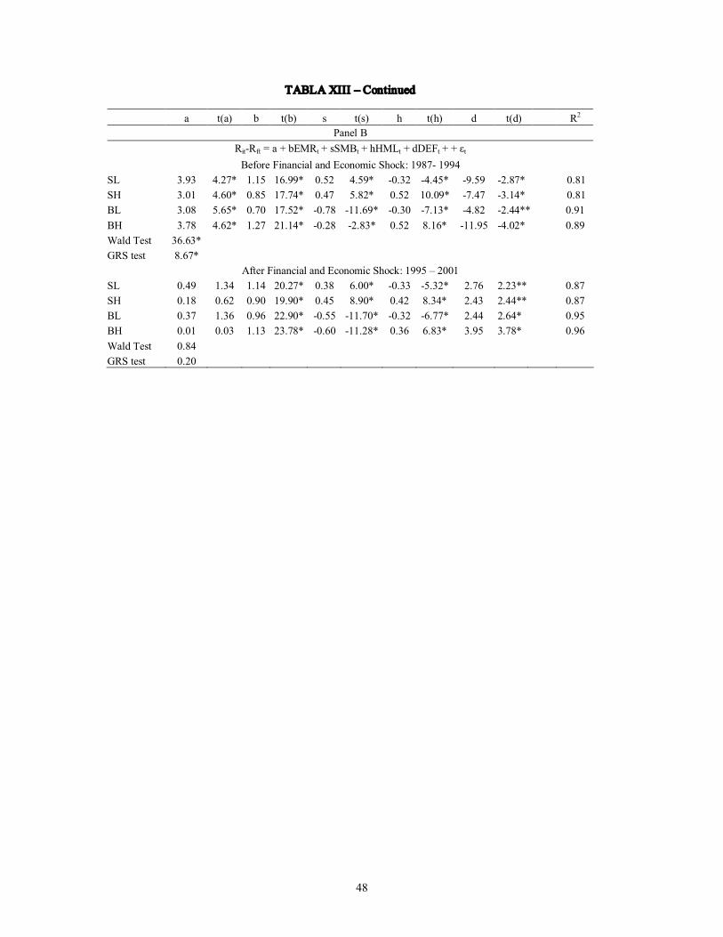
48
TABLA XIII – Continued
a t(a) b t(b) s t(s) h t(h) d t(d) R 2
Panel B RitRft = a + bEMRt + sSMBt + hHMLt + dDEFt + + εt Before Financial and Economic Shock: 1987 1994
SL 3.93 4.27* 1.15 16.99* 0.52 4.59* 0.32 4.45* 9.59 2.87* 0.81 SH 3.01 4.60* 0.85 17.74* 0.47 5.82* 0.52 10.09* 7.47 3.14* 0.81 BL 3.08 5.65* 0.70 17.52* 0.78 11.69* 0.30 7.13* 4.82 2.44** 0.91 BH 3.78 4.62* 1.27 21.14* 0.28 2.83* 0.52 8.16* 11.95 4.02* 0.89 Wald Test 36.63* GRS test 8.67*
After Financial and Economic Shock: 1995 – 2001 SL 0.49 1.34 1.14 20.27* 0.38 6.00* 0.33 5.32* 2.76 2.23** 0.87 SH 0.18 0.62 0.90 19.90* 0.45 8.90* 0.42 8.34* 2.43 2.44** 0.87 BL 0.37 1.36 0.96 22.90* 0.55 11.70* 0.32 6.77* 2.44 2.64* 0.95 BH 0.01 0.03 1.13 23.78* 0.60 11.28* 0.36 6.83* 3.95 3.78* 0.96 Wald Test 0.84 GRS test 0.20

49
TABLA XIV Regressions of Excess Por tfolio Returns on the Excess Market Return, Size Mimicking Por tfolio,
BooktoMarket Mimicking Por tfolio, Default Risk, Exchange Rate and Political Risk
I regressed for each subperiod (19871994, 19952001) the following time series regressions to estimate the coefficients αi and β’s for each of the four portfolios (SL, SH, BL and BH).
RitRft = a+bEMRt+sSMBt+hHMLt+dDEFt+ pPOLITICt + εt RitRft = a+bEMRt+sSMBt+hHMLt+eEXMt+ pPOLITICt + εt
RitRft is the excess return in each of the four portfolios, EMR is the excess market portfolio, SMB (small minus big) the size mimicking portfolio is the difference for each month between the simple average of the percent returns on the three smallstock portfolios (SL, SM, SH) and the simple average of the returns on the three big stock portfolios (BL, BM, BH). HML (high minus low) the booktomarket mimicking portfolio is the difference for each month between the simple average of the percent returns on the two highB/M portfolios (SH, BH) and the simple average of the returns on the two lowB/M portfolios (SL and BL). DEF is the default risk calculated as the spread between commercial paper rate and onemonth CETES rate and EXM is the monthly change in peso dollar exchange rate. POLITIC is the monthly return spread between a dollar bond issued by the Mexican and U.S. government. This table shows for each subperiod the coefficients (β’s), intercepts (αi), tstatistics values, R 2 , standard deviations s(e), Wald statistic and GRS statistic tests. *,** and *** indicate significance at 99, 95 and 90 percent level respectively
a t(a) b t(b) S t(s) h t(h) d t(d) P t(p) R 2
Panel A
RitRft = a + bEMRt + sSMBt + hHMLt + dDEFt + pPOLITICt + εt Before Financial and Economic Shock: 1987 1994
SL 3.51 3.71* 1.10 15.04* 0.51 4.56* 0.37 4.80* 9.48 2.86* 0.58 1.69*** 0.81 SH 2.73 4.05* 0.82 15.74* 0.46 5.80* 0.48 8.77* 7.38 3.13* 0.39 1.61*** 0.82 BL 3.40 6.15* 0.74 17.26* 0.77 11.83* 0.27 5.87* 4.91 2.53* 0.43 2.19** 0.92 BH 2.72 3.69* 1.14 20.05* 0.30 3.49* 0.40 6.55* 11.65 4.51* 1.44 5.41* 0.92 Wald Test 30.0* GRS test 5.6*
After Financial and Economic Shock: 1995 – 2001 SL 0.36 0.93 1.12 18.83* 0.38 6.05* 0.34 5.39* 3.02 2.37* 0.05 0.89 0.87 SH 0.07 0.22 0.88 18.47* 0.45 8.96* 0.41 8.04* 2.66 2.61* 0.04 1.01 0.87 BL 0.29 1.01 0.95 21.33* 0.54 11.54* 0.32 6.77* 2.59 2.73* 0.03 0.73 0.95 BH 0.18 0.55 1.10 22.16* 0.59 11.20* 0.35 6.53* 4.34 4.08* 0.07 1.61* 0.96 Wald Test 0.19 GRS test 0.04

50
TABLA XIV Continued
a t(a) b t(b) s t(s) h T(h) e t(e) p t(p) R 2
Panel B RitRft = a + bEMRt + sSMBt + hHMLt + eEXMt + pPOLITICt + εt
Before Financial and Economic Shock: 1987 1994 SL 3.16 4.44* 1.13 19.91* 0.44 5.16* 0.46 7.54* 2.10 8.49* 3.08 7.82* 0.89 SH 0.69 1.08 0.83 16.24* 0.42 5.46* 0.45 8.19* 0.82 3.69* 1.38 3.88* 0.83 BL 0.52 1.04 0.75 18.98* 0.80 13.34* 0.30 7.07* 0.82 4.80* 0.55 2.02** 0.93 BH 4.31 8.84* 1.17 30.18* 0.37 6.31* 0.31 7.44* 2.05 12.08* 3.89 14.39* 0.96 Wald Test 13.69* GRS test 0.00
After Financial and Economic Shock: 1995 – 2001 SL 0.03 0.08 1.08 18.79* 0.37 6.03* 0.35 5.70* 0.40 3.13* 0.57 3.11* 0.88 SH 0.10 0.78 0.85 17.70* 0.44 8.59* 0.42 8.10* 0.22 1.99** 0.31 2.03** 0.86 BL 0.35 1.07 0.92 20.42* 0.56 11.73* 0.31 6.43* 0.20 1.95** 0.27 1.91** 0.95 BH 0.54 1.60 1.05 22.26* 0.61 12.29* 0.34 6.69* 0.53 5.05* 0.76 5.06* 0.96 Wald Test 0.00 GRS test 0.00

51
TABLE XV Risk Factor s Cor relations: 19871994 and 19952001
This table presents the correlation coefficient. EMR is the excess market portfolio, SMB is the size mimicking portfolio, HML the booktomarket mimicking portfolio, DEF the default risk, EXM is the monthly change in pesodollar exchange rate, POLITIC is the monthly return spread between a dollar bond issued by the Mexican and U.S. government and TERM is the interest rate term structures.
EMR SMB HML DEF TERM EXM EMR SMB HML DEF TERM EXM Before Financial and Economic Shock:
19871994 After Financial and Economic Shock:
19952001 SMB 0.455 0.581 HML 0.115 0.148 0.004 0.006 DEF 0.053 0.109 0.041 0.199 0.014 0.236 TERM 0.080 0.023 0.082 0.212 0.259 0.024 0.192 0.069 EXM 0.373 0.205 0.125 0.320 0.532 0.431 0.286 0.033 0.383 0.431 POLITIC 0.370 0.210 0.315 0.051 0.456 0.779 0.473 0.318 0.101 0.248 0.452 0.966